Simulating deformable objects for computer animation: a numerical perspective

Abstract.

We examine a variety of numerical methods that arise when considering dynamical systems in the context of physics-based simulations of deformable objects. Such problems arise in various applications, including animation, robotics, control and fabrication. The goals and merits of suitable numerical algorithms for these applications are different from those of typical numerical analysis research in dynamical systems. Here the mathematical model is not fixed a priori but must be adjusted as necessary to capture the desired behaviour, with an emphasis on effectively producing lively animations of objects with complex geometries. Results are often judged by how realistic they appear to observers (by the “eye-norm”) as well as by the efficacy of the numerical procedures employed. And yet, we show that with an adjusted view numerical analysis and applied mathematics can contribute significantly to the development of appropriate methods and their analysis in a variety of areas including finite element methods, stiff and highly oscillatory ODEs, model reduction, and constrained optimization.

Uri M. Ascher^∗ and Egor Larionov and Seung Heon Sheen and Dinesh K. Pai

Dept. Computer Science

University of British Columbia

Vancouver, BC, V6T 1Z4, Canada

1. Introduction

Physics-based simulations of deformable objects are ubiquitous in computer graphics today. They arise in various applications including animation, robotics, control and fabrication. Whereas in typical numerical analysis research of dynamical systems the mathematical model is given and the task is to construct and prove the properties of computational methods that efficiently and reliably provide highly accurate solutions in often idealized circumstances, here the emphasis is typically on effectively producing lively-looking animations of objects with rather complex geometries (see Figure 1). The quality of the results is judged by the “eye-norm” as well as the efficacy of the numerical procedures employed. Numerical analysts and applied mathematicians thus can contribute significantly while adjusting to such a different environment, as the usual methods of scientific computing remain important and relevant and yet are not always ideal for a given task.

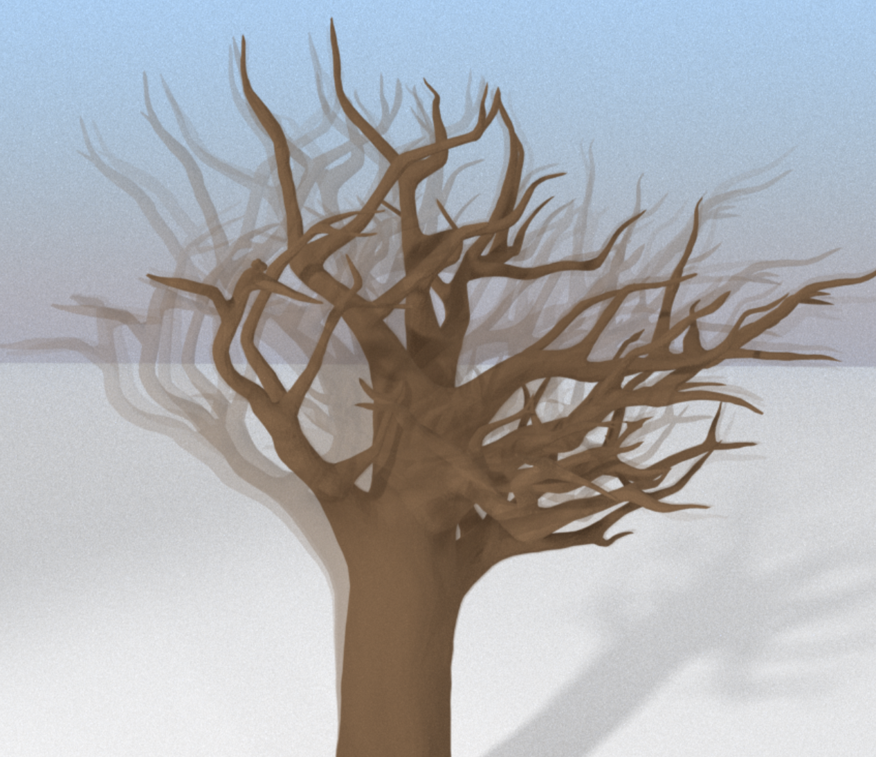
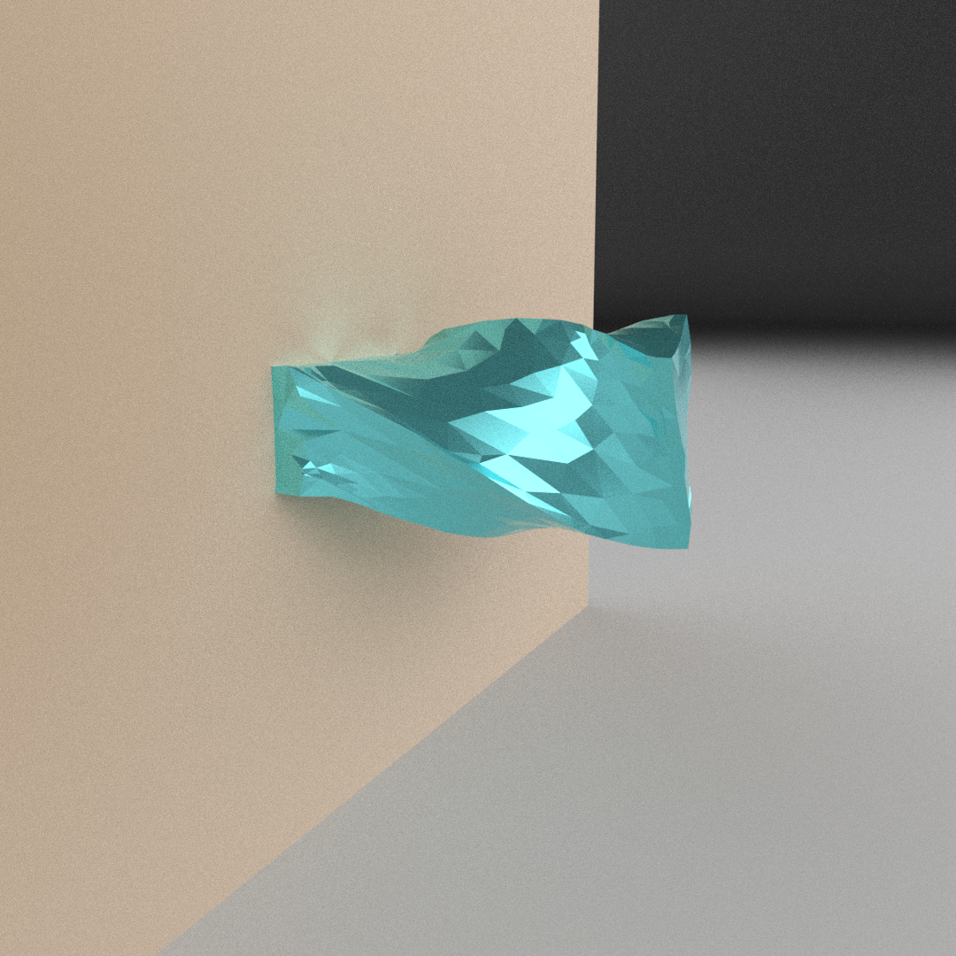
Figure 1. Deformable articulated objects: a swaying tree and a constrained jelly brick; cf. [13]

Example 1.

To demonstrate the issues involved, suppose that we have discretized in space the equations of motion for one of the objects in Figures 1 and 2 using a tetrahedral finite element mesh. Assuming only linear elastic forces ${\bf f}$, the equations of motion in time $t$ read

$$M\ddot{\bf q}={\bf f}({\bf q})=-K{\bf q}.$$ (1)

Here ${\bf q}(t)$ are the node coordinates of the finite elements, the corresponding accelerations are denoted by $\ddot{\bf q}$, $K$ is the stiffness matrix, and $M$ is the mass matrix. Assume that both of these matrices are constant and symmetric positive definite (SPD). Note that ${\bf q}$ is not a function of the mesh: rather, it consists of the mesh nodes; see Figure 2.

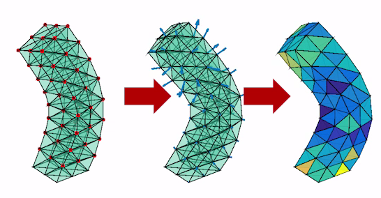
Figure 2. Moving tetrahedral FEM mesh for position coordinates ${\bf q}(t)$.

The matrix $K$ may well have large eigenvalues (which usually correspond to high frequency oscillations), both because upon using a fine spatial discretization higher and higher modes are captured and because the object’s material itself may be stiff (expressed by a large Young’s modulus).

In (1) we have a simple Hamiltonian system, and thus typical suitable time discretizations that may come to mind are conservative: they would be symmetric and non-dissipative (such as the trapezoidal rule), if not downright symplectic [23].

However, there is always some damping in the motion of such objects. Moreover, symplectic and symmetric time discretization methods cannot be L-stable [24], and much care is therefore required near boundary constraints such as contact [10]. In applied mathematics literature the damping force has traditionally been handled by adding to ${\bf f}$ a Rayleigh damping force term

$${\bf f}_{\rm dmp}({\bf q},\dot{\bf q})=(\alpha K+\beta M)\dot{\bf q},$$ (2)

where $\alpha>0$ and $\beta\geq 0$ are suitable constants. However, the Rayleigh damping, although theoretically rather helpful, does not cover all manners of motion behaviour observed in practice. Even though there has been work in measuring material properties of real objects [41] and even humans [42], the selection of suitable damping parameters (as is the choice of parameters in (2)) in different practical circumstances remains a challenging problem that is often solved by trial and error (e.g., [49]).

In the computer graphics literature, in contrast to the above, the semi-implicit backward-Euler (SI) method of Baraff and Witkin [6] has been widely employed. This method allows for stable simulations even when large time steps are used for efficiency reasons, and it is very stable when incorporating contacts and collisions due to its heavy damping and error localization properties. Moreover, numerical damping is in agreement with the observation that our visual system does not detect high frequency vibrations, even when objects with large Young’s modulus are simulated.

And yet, recent years have also seen growing concerns that heavy numerical damping may be unsuitable for many purposes, because it can only be controlled via the time step size, so it does not distinguish phenomena related to material heterogeneity and more complex damping forces [15, 11]. Animations produced using such methods often do not appear to be sufficiently lively. Use of the SI method in applications such as control and fabrication, where more faithfulness to physics is desired, has also been considered debatable [10].

A further concern that arises when the force ${\bf f}$ is nonlinear is that SI has long been known to occasionally diverge wildly where the fully implicit backward Euler (BE) still yields acceptable results. This ushers another issue seldom considered seriously in the geometric numerical integration community, namely, finding solution methods for the nonlinear systems of algebraic equations that typically arise in the present context.

In this paper we consider several issues that involve the transportation of methods and ideas from the numerical community to the present computer animation context. Following a short discussion in Section 2 of the equations of motion that arise from an FEM semi-discretization, we present and analyze in Section 3 several suitable methods for the stiff dynamical systems that arise. These include difference methods and exponential ones, as well as additive methods that involve both through a model reduction algorithm. Numerical experiments with soft objects are reported in Section 4, and methods for handling contact and friction constraints are considered in Section 5. These involve several interesting modelling and optimization issues. Conclusions are offered in Section 6.

Virtually all research papers on the present topic in the computer graphics and robotics literature are supplemented by video clips that demonstrate object motion obtained by the proposed numerical methods. Such material can usually be accessed through authors’ project pages, home pages, or even YouTube on the web. Our own relevant videos for [11, 13, 12] and [28], respectively, can be found at
https://www.youtube.com/watch?v=oRGuC9GMm8w
https://www.cs.ubc.ca/$\sim$ascher/papers/csap.m4v
https://www.youtube.com/watch?v=aIAKBsT96to&feature=youtu.be
https://elrnv.com/vid/fcses_tog2021.webm

2. Motion of deformable objects

A common approach for discretizing an elastodynamic system is to first apply a finite element method (FEM) in space, already at the variational level. Usually in physics-based animations linear element basis functions are used on tetrahedra (or less frequently, hexahedra), although there are works that employ higher degree elements [32]. The short course by Sifakis and Barbic [43] is a good introduction for this material and much more. See [16] for an exhaustive mathematical treatment of elasticity.

This spatial discretization results in a large ordinary differential equation (ODE) system in time $t$, written in standard notation as

$$M\ddot{{\bf q}}={{\bf f}}_{\rm tot}({\bf q},{\bf v}),$$ (3a)

where the unknowns $${\bf q}={\bf q}(t) {\bf v}(t)=\dot{\bf q}(t) M$$ are nodal displacements in the FEM mesh with corresponding nodal velocities . The mass matrix is SPD and sparse. The total force is further written as

$${\bf f}_{\rm tot}={{\bf f}}_{\rm els}({\bf q})+{{\bf f}}_{\rm dmp}({\bf q},{\bf v})+{{\bf f}}_{\rm con}({\bf q},{\bf v})+{{\bf f}}_{\rm ext}({\bf q}),$$ (3b)

where $${{\bf f}}_{\rm els}({\bf q}) {{\bf f}}_{\rm dmp}({\bf q},{\bf v}) {{\bf f}}_{\rm con} {{\bf f}}_{\rm ext}$$ are elastic forces, are damping forces (e.g., as given in (2)), are forces due to contact and friction constraints, and are external forces such as gravity.

The choice of spatial FEM discretization generally affects the resulting animations obtained by any subsequent numerical treatment of the semi-discretization (3), see for instance [10, 12]. Nonetheless, unlike in some shock wave calculations, there is enough separation between space and time here to allow a separate treatment of (3), and we proceed to do this following almost all relevant literature.

The elastic and damping forces are written as

$${{\bf f}}_{\rm els}({\bf q}(t))=-\frac{\partial}{\partial{\bf q}}W({\bf q}(t)),\quad{{\bf f}}_{\rm dmp}({\bf q}(t),{\bf v}(t))=-D{\bf v}(t),$$

where $W({\bf q}(t))$ is the elastic potential of the corresponding hyperelasticity model. We further define the tangent stiffness matrix $K=-\frac{\partial}{\partial{\bf q}}{\bf f}_{\rm els}({\bf q}(t)).$ This matrix is constant and SPD if ${\bf f}_{\rm els}$ is linear, but for nonlinear elastic forces it depends on the unknown ${\bf q}(t)$ and may occasionally become indefinite. Note that $K$ is possibly very large in size: fortunately, it is also rather sparse.

Typical nonlinear elastic forces include neo-Hookean, StVK and Mooney-Rivlin [16]. Nonlinear force effects in computer graphics include in addition as-rigid-as-possible (ARAP) forces [45], artist-generated forces, and co-rotated FEM, which is an FEM specialty not typically known to general FEM experts! (See, e.g., [47].)

The damping matrix $D=D({\bf q}(t))$ is symmetric nonnegative definite at all times, as in (2); see, for instance, [7, 16, 43, 10, 11].

A similar-looking problem arises upon using a mass-spring system [6, 8], though the spectrum of the corresponding stiffness matrix is less challenging to split in that case.

The ODE system in (3) can be written as a first-order system

$$\dot{{\bf u}}(t)\equiv\begin{bmatrix}\dot{{\bf q}}\\ \dot{{\bf v}}\end{bmatrix}=\begin{bmatrix}{0}&I\\ -M^{-1}K&-M^{-1}D\end{bmatrix}\begin{bmatrix}{\bf q}\\ {\bf v}\end{bmatrix}+\begin{bmatrix}\bf{0}\\ {{\bf c}}\end{bmatrix}\equiv{\bf F}({\bf u}).$$ (4)

The split form of writing these equations expresses an expectation that the remainder term ${\bf c}=M^{-1}({\bf f}_{\rm tot}+K{\bf q}+D{\bf v})$ is somehow dominated by the first term. Let us denote the (often large) length of ${\bf u}$ by $n$. In the tree example of Figure 1, $n\approx 180,000$. In industrial applications $n$ can get to millions.

Note that we could have avoided $M^{-1}$ in (4) by considering momenta ${\bf p}=M{\bf v}$. However, in the application domain considered here the mass matrix is often diagonal and simple, and the velocities are of direct interest.

3. Efficient simulation methods for stiff objects

In this section we mention and discuss several favourite time discretization methods that have seen use in practice. See also the recent [33].

3.1. Finite difference methods

Our prototype ODE problem (4) must be discretized before simulation. Let us concentrate on one time interval, stepping from time $t=t_{0}$ where we know an approximate solution ${\bf u}_{0}\approx{\bf u}(t_{0})$ to the next time level $t_{1}=t_{0}+h$ where the unknown approximation ${\bf u}_{1}\approx{\bf u}(t_{1})$ is sought.

The time step size $h$ is typically large, and it is kept constant as the simulation proceeds. This is in contrast to canned initial value ODE software, where usually the step size is adapted at each step, chosen so as to satisfy an equidistribution of a local error estimate [4, 24]. But here, the time step often has a physical meaning and is tied to a constant rate of operation of some physical apparatus, especially in robotics. Moreover, the meaning of “accuracy” is more relaxed in the present context compared to what numerical analysts are used to.

For instance, the backward Euler (BE) method is given by

$${\bf u}_{1}={\bf u}_{0}+h{\bf F}({\bf u}_{1}).$$ (5)

A large nonlinear system of algebraic equations must be solved for ${\bf u}_{1}$ when employing an implicit method such as (5). For this purpose Newton’s method for finding a root of

$${\bf g}({\bf u}_{1})={\bf u}_{1}-h{\bf F}({\bf u}_{1})-{\bf u}_{0}={\bf 0}$$

decrees iteration to convergence of

$${\bf u}_{1}^{(s+1)}={\bf u}_{1}^{(s)}-[I-hJ({\bf u}_{1}^{(s)})]^{-1}({\bf g}({\bf u}_{1}^{\color[rgb]{0,0,0}})),\quad s=0,1,\ldots$$

where the Jacobian matrix $J=\frac{\partial{\bf F}}{\partial{\bf u}}$ is large and sparse. This iteration may require careful control and possible modification in practice.

The SI method is derived by applying to BE just one Newton iteration starting at ${\bf u}_{1}^{(0)}={\bf u}_{0}$, obtaining

$${\bf u}_{1}={\bf u}_{0}+h[I-hJ({\bf u}_{0})]^{-1}{\bf F}({\bf u}_{0}).$$ (6)

For a linear ODE, BE and SI are the same; but for nonlinear forces and large step sizes $h$ they can differ significantly.

In the sequel we retain the notation SI for the semi-implicit version of BE. But of course a semi-implicit version can be obtained in the same fashion for any implicit difference method. We will distinguish such methods by adding the letter ’S’ in front of the method’s name. For instance, the BDF2 method is a two-step method that requires also the past approximation ${\bf u}_{-1}$ at $t_{0}-h$. This method reads

$${\bf u}_{1}={\bf u}_{0}+\frac{1}{3}\left({\bf u}_{0}-{\bf u}_{-1}+2h{\bf F}({\bf u}_{1})\right),$$ (7)

and its semi-implicit version is denoted by SBDF2.

As stated above, the popular SI method and even implicit integrators such as BE and higher order backward differentiation formulae (BDF) introduce significant, step-size dependent, artificial damping. All BDF methods collocate the ODE system only at the unknown time level. This typically yields a potentially heavy damping of high frequency modes that has often been observed and used to advantage in practice [11, 13].

Let us next discuss two diagonally implicit Runge-Kutta (DIRK) methods [2, 24, 29]. The TR-BDF2 method is motivated by wanting to use BDF2 over just one time step rather than two, making it a one-step method. But for this, a value for the solution at $t_{0}+h/2$ is required. This approximation is obtained using the trapezoidal rule (which by itself introduces no artificial damping), giving the method

$${\bf u}_{1/2} = {\bf u}_{0}+\frac{h}{4}\left({\bf F}({\bf u}_{1/2})+{\bf F}({\bf u}_{0})\right)$$ (8a)

$${\bf u}_{1} = {\bf u}_{0}+\frac{4}{3}({\bf u}_{1/2}-{\bf u}_{0})+\frac{h}{3}{{\bf F}}({\bf u}_{1}).$$ (8b)

This method performed well in comparative experiments reported in [33]. It has two implicit stages, each requiring the solution of a nonlinear system of size $n$. S-versions for these are derived directly as before. In fully implicit $r$-stage RK methods a nonlinear system of size $rn$ must be solved, and this is avoided here by the DIRK method. The matrices to be inverted (or rather, decomposed) here, similarly to (6), are $I-\frac{h}{4}J$ and $I-\frac{h}{3}J$. A nearby singly DIRK (SDIRK, where ’S’ here stands for ’singly’, not ’semi’) method uses the trapezoidal rule to advance to $t_{0}+\gamma h$ first, where $\gamma=2-\sqrt{2}$. This yields the method

$${\bf u}_{\gamma} = {\bf u}_{0}+\frac{\gamma h}{2}\left({\bf F}({\bf u}_{\gamma})+{\bf F}({\bf u}_{0})\right)$$ (9a)

$${\bf u}_{1} = {\bf u}_{0}+\frac{2\beta}{\gamma}({\bf u}_{\gamma}-{\bf u}_{0})+\frac{\gamma h}{2}{{\bf F}}({\bf u}_{1}),$$ (9b)

where $$\beta=\frac{\sqrt{2}}{4}$$.

The corresponding Butcher Tableau representation for the methods (8) and (9) is

$$\begin{array}[]{r|rrr}0&&&\\ 1/2&1/4&1/4&\\ 1&1/3&1/3&1/3\\ \hline\cr&1/3&1/3&1/3\end{array}\quad{\rm~{}~{}and~{}~{}}\quad\begin{array}[]{r|rrr}0&&&\\ \gamma&\frac{\gamma}{2}&\frac{\gamma}{2}&\\ 1&\beta&\beta&\frac{\gamma}{2}\\ \hline\cr&\beta&\beta&\frac{\gamma}{2}\end{array}$$

respectively. In the sequel we will refer for simplicity to (9) as the SDIRK method: there is no other SDIRK method in this paper to get confused by.

The advantage of the SDIRK method (9), favoured in the initial value ODE literature [2, 24, 9], is that it can be implemented somewhat more efficiently, because upon freezing the Jacobian matrix $J$ over the step’s interval, we get to invert the same matrix $I-\frac{\gamma h}{2}J$ en route to solving the two nonlinear problems in the stages of (9). The same LU decomposition may then be used for both stages. This advantage fades away if an iterative solution method must be employed for this large problem. The order of accuracy in both stages of these methods equals $2$, and they can both be shown to be L-stable [24, 9, 29, 4]. For (8), in particular, upon considering the test equation $\dot{u}=\lambda u$ for a complex scalar $\lambda$ and writing the resulting step as $u_{1}=R(z)u_{0}$ with $z=\lambda h$, it is not difficult to show that

$$R(z)\approx 5/z\rightarrow 0\quad{\rm as~{}}|z|\rightarrow\infty.$$

L-stability follows.

On the other hand, for very stiff problems both of these DIRK variants share a disadvantage, as the following example shows.

Example 2.

Consider the test equation

$$\dot{u}=-1000u,\quad u(0)=1,$$

and use a step of size $h=.1$, say, to advance the first step (i.e., $t_{0}=0$). Applying the BDF2 method to this yields $u_{1}>0$ that is close to $0$ but still nonnegative. However, the trapezoidal method in both (8a) and (9a) would yield a negative $u_{\gamma}\approx-1$.

Now consider the ODE system for ${\bf u}(t)=(u,w)^{T}$, given by

$$\dot{u}=-1000u,\;\;\dot{w}=\log(u).$$

The BDF2 method will complete the step successfully, whereas both featured DIRK methods will get stuck, being unable to evaluate $\log(u_{\gamma})$ for calculating $w_{1}$.

For mildly stiff problems, typically bad effects such as instability accumulate over several time steps. However, in very stiff problems like the one under consideration here, a method such as trapezoidal could already cause irreparable inaccuracy over just half a step, thus not allowing the BDF2 that follows a chance to fix things up.

3.2. Damping curves

The test equation used to draw stability regions and define concepts such as A-stability and L-stability [24, 4] is less natural when it comes to analyzing the second-order problem in Example 1 or more generally the system (3). Instead we consider the scalar ODE

$$\ddot{q}+\omega^{2}q=0,$$ (11)

where $\omega$ is a potentially large frequency. See [11, 13, 14].

Rewriting (11) as a first order system and applying a difference discretization such as any of the methods described above, we can write the operation over one time step as

$${\bf u}_{1}=T{\bf u}_{0},$$

where $T$ is a constant transformation matrix (of size $2\times 2$ for a one-step method). The spectral radius of $T$, $\rho(T)$, then corresponds to $|R(z)|$ above, as it gives the contraction factor in $\|{\bf u}\|$. Of course, in (11) the oscillations are undamped, so we expect damping numerical methods such as all of the above to approximate more closely the solution of the modified ODE

$$\ddot{q}+d^{\rm method}\dot{q}+\omega^{2}q=0,$$ (12)

where the damping coefficent $d^{\rm method}\geq 0$ depends on $\omega$ and $h$ in such a way that $d^{\rm method}/\omega$ depends only on the product $\omega h$. The (simple) procedure for determining $d^{\rm method}$ is described in Section 3.1 of [11].

Of course, for conservative discretizations such as trapezoidal, implicit midpoint, collocation at Gaussian points, and Kane’s method [25] there is no artificial damping and $d^{\rm method}=0$. But for damping methods we can obtain telling tales in this fashion. Figure 18 in [13] shows that the BE damping curve $d^{\rm BE}$ has a similar shape as $d^{\rm BDF2}$, but the damping is roughly twice as large in magnitude. An interesting comparison of the DIRK methods and BDF2 (all 2nd order methods) is presented in Figure 3 below.

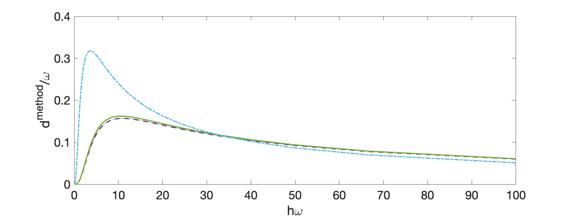
Figure 3. Damping curves for the SDIRK method (solid line), TR-BDF2 (dashed) and BDF2 (dash-dot). The two DIRK methods behave similarly, and they differ significantly from BDF2.

Clearly, the two DIRK methods are close to each other in this respect as well, with TR-BDF2 (8) damping slightly less. The BDF2 curve, on the other hand, suggests significantly more damping around $h\omega\approx 1$ and less when $h\omega\gg 1$. The DIRK curves are more appealing, in fact, implying less dependence on the frequency as well as less damping for low frequencies.

3.3. Solving the nonlinear algebraic equations

Curiously, in situations where there is a real need to solve the nonlinear equations arising from implicit discretizations of the problem (3), or (4), this may become a challenge. Among the reasons are the sheer size of the problem, the fact that large steps are considered so ${\bf u}_{0}$ may not be a close approximation to ${\bf u}_{1}$, and the observation that we are considering situations where the semi-implicit version (i.e., one Newton iteration) is not sufficient.

A general approach for solving systems of nonlinear equations is to cast this as an optimization problem; cf. [21]. We may always consider minimizing a scaled $\ell_{2}$-norm of the residual. For instance, applied to BE (5) this reads

$$\min_{{\bf u}_{1}}\phi_{LSBE}=\frac{1}{2}\|B({\bf u}_{1}-{\bf u}_{0}-h{\bf F}({\bf u}_{1}))\|,$$ (13)

where the scaling matrix $B$ multiplying the residuals in this expression may depend on the time step. It can be the identity, or a diagonal matrix that scales the rows, or even the inverse of a Jacobian evaluated once at the beginning of the time step.

The advantages of such formulations are that they are general in terms of the forces regardless of integrability, and that constraints may be added directly to form a constrained optimization problem. A disadvantage, however, is that the gradient expression involves $J^{T}J$, and this reduces the sparsity of the Jacobian and squares its condition number.

An alternative option is to employ a damped Newton strategy, using (13) (and its likes for other implicit discretizations) only as a merit function. But let us stay with the “lazy option” of just employing an optimization software package for our present problem.

To simplify matters, let us consider just elastic forces in (3b). This force is integrable, and we have ${\bf f}_{\rm tot}=-\frac{\partial W({\bf q})}{\partial{\bf q}}$ with $W$ the potential energy. Thus we can write the nonlinear equations ${\bf u}_{1}={\bf u}_{0}+h{\bf F}({\bf u}_{1})$ for BE as the necessary condition for a minimum of

$$\min_{{\bf v}_{1}}\phi_{BE} \equiv \frac{1}{2}\|{\bf v}_{1}-{\bf v}_{0}\|_{M}^{2}+W({\bf q}_{1}),$$ (14)

$${\rm where}~{}~{}{\bf q}_{1} = {\bf q}_{0}+h{\bf v}_{1}.$$

See, e.g., [30]. Here we have used the “energy norm” $\|{\bf v}\|_{M}=\sqrt{{\bf v}^{T}M{\bf v}}$ for the kinetic energy term.

A similar, if slightly more complex, expression can be written for BDF2: The nonlinear equations ${\bf u}_{1}={\bf u}_{0}+\frac{1}{3}\left({\bf u}_{0}-{\bf u}_{-1}+2h{\bf F}({\bf u}_{1})\right)$ are written as the necessary condition for a minimum of

$$\min_{{\bf v}_{1}}\phi_{BDF2} \equiv \frac{1}{2}\|{\bf v}_{1}-\tilde{\bf v}\|_{M}^{2}+W({\bf q}_{1}),$$ (15)

$${\rm where}~{}~{}{\bf q}_{1} = {\bf q}_{0}+\frac{1}{3}\left({\bf q}_{0}-{\bf q}_{-1}+2h{\bf v}_{1}\right),$$

$${\rm with}~{}~{}\tilde{\bf v} = {\bf v}_{0}+\frac{1}{3}({\bf v}_{0}-{\bf v}_{-1}).$$

Method-dependent optimization problems can be similarly constructed also for other discretization methods, including trapezoidal and the DIRK methods. An advantage in these objective functions is that no matrix sparsity is sacrificed. Other integrable forces such as gravity and frictionless contact forces can be handled in a similar way: see Section 5. An explicitly stated damping force can be a bit more tricky and require some approximation such as freezing $D$.

3.4. Newmark methods

Newmark methods are very popular in structural mechanics and related fields, less so in the numerical ODE community. Generalized $\alpha$ is one such family of methods that has been used in computer graphics applications. It has a knob (parameter) to control the amount of artificial diffusion per frequency [15]. These methods are one-step and $2$nd order accurate.

Let us rewrite the ODE (3) as a simple semi-explicit differential-algebraic equation (DAE):

$$\dot{\bf q}={\bf v},\quad\dot{\bf v}={\bf a},\quad{\bf 0}=M{\bf a}-{\bf f}_{\rm tot}({\bf q},{\bf v}).$$ (16)

The time step unknowns from $t_{0}$ to $t_{1}$ are ${\bf q}_{1},{\bf v}_{1}$ and ${\bf a}_{\nu}$, i.e., it is a staggered time stepping for the acceleration, where $\nu$ is a parameter. See [11] for further details, including damping curves for the generalized $\alpha$ method. These curves are comparable to those of a simple mixture of the trapezoidal and BDF2 methods. Our experiments, as well as those of others, have not left us with the feeling that there is much additional uplift to look for here, although these methods are solid performers in general.

3.5. Exponential methods

Instead of finite difference discretizations as described above, one can resort to exponential methods. Such methods are more accurate when they work, and they approximate the entire modal spectrum with little artificial damping (indeed, $d^{\rm method}\equiv 0$ in the modified test equation (12)). Moreover, these methods are semi-implicit rather than fully implicit, and require no solutions of nonlinear algebraic equations!

Several exponential integration schemes have been proposed in the computer graphics literature; see [37, 36, 11] and references therein. In principle they all involve calculations of the action of the matrix exponential of $M^{-1}K$ on various vectors.

3.5.1. ERE

The exponential Rosenbrock Euler (ERE) method of [11] is particularly suitable for nonlinear forces in some challenging situations. Its nominal order is commensurate with that of the BE method, although it is generally much more accurate than BE.

With the Jacobian $J$ defined as before we first write (4) as

$$\dot{\bf u}={\bf F}({\bf u})=J{\bf u}+{\bf c}({\bf u}),\;\quad{\rm where}\;\;J=\frac{\partial{\bf F}}{\partial{\bf u}},$$ (17)

so ${\bf c}({\bf u})$ is nonlinear but hopefully can be treated as an inhomogeneity. Next, write the step from $t_{0}$ to $t_{1}$ as approximating the integral form of (17) over one step

$${\bf u}(t_{1})=\text{exp}(hJ){\bf u}_{0}+\int_{t_{0}}^{t_{1}}\text{exp}((t_{1}-s)J){\bf c}({\bf u}(s))\text{d}s.$$

This yields the ERE step

$${\bf u}_{1} = {\bf u}_{0}+h\phi_{1}(hJ){\bf F}({\bf u}_{0}),\quad{\rm with}$$ (18a)

$$\phi_{1}(Z) = Z^{-1}(\exp(Z)-I).$$ (18b)

The remaining key issue is the evaluation of the product of $\phi_{1}(hJ)$ times a vector. Of special concern is the exponential matrix $\exp(hJ)$, which is very large and unfortunately no longer sparse. This is discussed in detail in [11]. A Krylov-space method is employed there for the implementation used for approximating the product of $\exp(hJ)$ with vectors ${\bf F}$ [38, 39, 1].

3.5.2. SIERE

The method used in  [11] for calculating $\exp(hJ){\bf F}$ is efficient for objects made of material that is not very stiff. However, as shown in Figure 4, these methods become expensive for stiff problems, because the required number of Krylov vectors can become very large. Thus, the utility of exponential integrators in the context of stiff deformable object simulations is limited. The method proposed in [13] alleviates this difficulty by applying ERE only in a suitable subspace, and the exponential matrix evaluation at each time step is drastically simplified due to matrix diagonalization.

\begin{overpic}[width=180.67499pt,trim=0.0pt 0.0pt 15.05624pt 0.0pt,clip]{swinging_arma_cost2.pdf} \put(10.0,30.0){\includegraphics[width=54.20029pt]{swinging_arma0}} \put(100.0,42.0){\rotatebox[origin={c}]{90.0}{\footnotesize Run Time (seconds)}} \end{overpic}

Figure 4. Computational costs for a swinging armadillo simulation [13]. The cost of exponential integrators including ERE becomes prohibitive as the stiffness parameter increases. By contrast, the cost of SIERE does not grow significantly with stiffness.

Observe at first that the advantages and disadvantages of ERE and SI are largely complementary. SI is cheap and stable, and its efficiency does not deteriorate for highly stiff problems; yet it is lethargic and loses energy rapidly, and it may exhibit divergence for large steps when BE is not approximated well. On the other hand, ERE approximates all modes reasonably well, and it is also semi-implicit; but its performance deteriorates for very stiff problems. So, SIERE combines these two methods such that ERE works on the $s$ lowest modes while SI is applied to dampen the higher modes. Typically, $1\leq s\leq 20$, with $s=5$ being already suitable for many practical applications.

We employ the additive method framework: If ${\bf F}({\bf u})$ can be written for each time instance $t$ as a sum of two parts

$${\bf F}({\bf u}(t))={\bf H}({\bf u}(t))+{\bf G}({\bf u}(t)),$$ (19)

then we can apply different integration schemes for ${\bf H}$ and for ${\bf G}$. Combining BE and ERE in this way gives the method BEERE, defined by

$${\bf u}_{1}={\bf u}_{0}+h{\bf H}({\bf u}_{1})+h\phi_{1}(hJ_{G}){\bf G}({\bf u}_{0}),$$ (20)

while SIERE is defined upon approximating BE by its semi-implicit iteration

$${\bf u}_{1}={\bf u}_{0}+(I-hJ_{H})^{-1}(h{\bf H}({\bf u}_{0})+h\phi_{1}(hJ_{G}){\bf G}({\bf u}_{0})).$$ (21)

We can of course combine other methods with ERE this way. For instance, the BDF2ERE method is defined by

$$\hat{\bf u} = \frac{1}{3}\left(4{\bf u}_{0}-{\bf u}_{-1}+2h\phi_{1}(hJ_{G}){\bf G}({\bf u}_{0})\right),$$ (22a)

$${\bf u}_{1} = \hat{\bf u}+\frac{2h}{3}{\bf H}({\bf u}_{1}),$$ (22b)

and its semi-implicit version is

$${\bf u}_{1} = \hat{\bf u}+\frac{2h}{3}({\bf H}({\bf u}_{0})+J_{H}({\bf u}_{1}-{\bf u}_{0}))$$ (23)

$$= {\bf u}_{0}+\frac{1}{3}(I-\frac{2h}{3}J_{H})^{-1}\left({\bf u}_{0}-{\bf u}_{-1}+2h{\bf H}({\bf u}_{0})+2h\phi_{1}(hJ_{G}){\bf G}({\bf u}_{0})\right).$$

The SBDF2ERE method given in (23) is only slightly more expensive than SIERE.

The above methods from (20) to (23) can be naturally viewed as splitting methods as well; see, e.g., [3].

The splitting of ${\bf F}({\bf u})$ as in (19) is achieved in [13] using a model reduction technique. Assuming that the dominant part of the force ${\bf f}_{\rm tot}$ is in $-M^{-1}K{\bf q}$, the Fourier ansatz ${\bf q}(t)={\bf x}\exp(\imath\sqrt{\lambda}t)$ at each step start $t=t_{0}$ gives the generalized eigenvalue problem

$$K({\bf q}(t_{0})){\bf x}=\lambda M{\bf x}.$$

With $X_{s}$ the (long and skinny) matrix of first $s$ eigenmodes and $D_{s}={\rm diag}~{}[\lambda_{1},\ldots,\lambda_{s}]$ we obtain

$$KX_{s}=MX_{s}D_{s}.$$

Next, define

$${\bf G}({\bf u})=\begin{bmatrix}{\bf v}_{G}\\ M^{-1}{\bf f}_{G}\end{bmatrix}\quad{\bf H}({\bf u})=\begin{bmatrix}{\bf v}_{H}\\ M^{-1}{\bf f}_{H}\end{bmatrix},$$

where ${{\bf v}_{G}=X_{s}X_{s}^{T}M{\bf v}},\ {\bf v}_{H}={\bf v}-{\bf v}_{G},\ {{\bf f}_{G}=MX_{s}X_{s}^{T}{\bf f}},\ {\bf f}_{H}={\bf f}-{\bf f}_{G}$. It follows that

$$J_{G}=\begin{bmatrix}0&X_{s}X_{s}^{T}M\\ -X_{s}X_{s}^{T}KX_{s}X_{s}^{T}M&0\end{bmatrix}\quad J_{H}=\begin{bmatrix}0&I\\ -M^{-1}K&0\end{bmatrix}-J_{G}.$$ (24)

For the ERE update in the subspace we write

$${\bf u}_{1}={\bf u}_{0}+h(I-hJ_{H})^{-1}\left({\bf H}({\bf u}_{0})+\begin{bmatrix}X_{s}&0\\ 0&X_{s}\end{bmatrix}\phi_{1}(hJ^{r}_{G}){\bf G}^{r}({\bf u}_{0})\right),$$ (25a)

where

$$J^{r}_{G}=\begin{bmatrix}0&I\\ -X_{s}^{T}KX_{s}&0\end{bmatrix}\quad{\bf G}^{r}({\bf u})=\begin{bmatrix}X_{s}^{T}M{\bf v}\\ X_{s}^{T}{\bf f}\end{bmatrix}.$$ (25b)

Note that the ERE expression $$h\phi_{1}(hJ_{G}){\bf G}({\bf u}_{0})$$ can be trivially evaluated in the subspace first and then projected back to the original space.

Sifting through the suddenly detailed expressions above, we note the crucial point that in (25a) the very large linear algebraic system that must be solved involves the matrix $I-hJ_{H}$ which is no longer sparse. Fortunately, this matrix is an $s$-rank correction of the sparse matrix $I-hJ$

$$I-hJ_{H}=(I-hJ)+h\left(Y_{1}Z_{1}^{T}+Y_{2}Z_{2}^{T}\right),$$ (26)

where $J$ is a typically sparse FEM matrix and $Y_{i}$ and $Z_{i}$ are skinny $n\times s$ matrices. This saves the day, in principle:

• For iterative methods (e.g., conjugate gradient) evaluating
  $J_{H}{\bf w}=J{\bf w}+Y_{1}\left(Z_{1}^{T}{\bf w})+Y_{2}(Z_{2}^{T}{\bf w}\right)$ for any given vector ${\bf w}$ is efficient.

• For direct methods (i.e., variants of Gaussian elimination) we employ the celebrated Sherman-Morrison-Woodbury (SMW) formula

  $$\left(A+YZ^{T}\right)^{-1}=A^{-1}-A^{-1}Y\left(I+Z^{T}A^{-1}Y\right)^{-1}Z^{T}A^{-1}$$

  for $A=I-hJ$.

See [13] for more details and extensive demonstration of the efficacy of SIERE.

Other hybrid methods such as BEERE and BDF2RE require the solution of nonlinear algebraic equations at each time step. Note that (22b) looks just like BE, and such is the case also for the nonlinear part of (20). Hence the optimization methods decribed in Section 3.1, in particular (14), can be adapted to include BEERE and BDF2ERE. There is a catch, though, in that the procedures for evaluating $(I-J_{H}){\bf w}$ and $(I-J_{H})^{-1}{\bf w}$ for any given vector ${\bf w}$ are specialized, so care must be exercised when using canned optimization software. We feel that the exciting development here is rather in the semi-implicit variants SIERE and SBDF2ERE. For instance, with an appropriate choice of $s$, the semi-implicit expression for $\hat{\bf u}$ in (22a) often gives a sufficiently good approximation for ${\bf u}_{1}$ so that one subsequent Newton iteration for (22b), i.e., SBDF2ERE, suffices!

4. Efficient simulation methods for soft objects

Soft objects, such as the characters that appear in animation movies aimed at young audiences, commonly arise in computer graphics applications. Here, the DIRK methods introduced in Section 3.1, namely TR-BDF2 and SDIRK, have a good record [49, 33], even though occasionally an additional stabilization or damping may be required.

For soft objects with nonlinear elastic forces, there may be large deformations during a single time step that change the eigenvalues and modes described above significantly, enough to cause the eigenmodes to cross [12]. If contemplating use of additive methods such as SIERE, then for stiff objects it is sufficient to perform the spectral decomposition only once, at the beginning. However, for soft objects, one may need to perform the spectral decomposition more frequently, possibly even at every frame (i.e., time step interval). Doing this does produce more stable results in our experiments, but at the cost of increased runtime, since computing the first $s$ eigenpairs is significantly more expensive than the other parts of the integrator within one time frame. Such additional cost is still small compared to just assembling the forces and the stiffness matrix at each time step, though. This raises the question of how frequently one should compute this decomposition without sacrificing too much compute time while still remaining faithful to the simulated deformation.

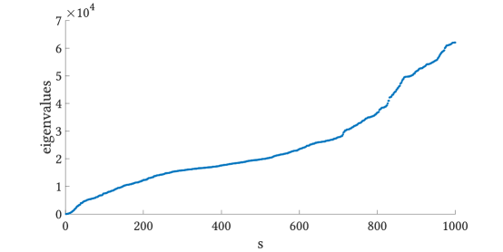
Figure 5. Plot of of the first 1000 eigenvalues of a soft body problem.

Another issue is that for soft problems it can be hard to clearly distinguish the first $s$ low frequency modes from higher ones for a small $s$. Consider Figure 5, where we plot the first $1000$ eigenvalues for a soft body problem. Here, there is no clear separation in the eigenvalues, and it is hard to clearly distinguish a small number of lowest eigenmodes that dominate the dynamics. In other words, more eigenmodes play a significant role in the visible dynamics.

\begin{overpic}[width=361.34999pt]{beam_energy_1.pdf} \put(25.0,30.0){\includegraphics[scale={0.08}]{rep.png}} \end{overpic}

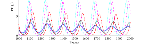
Figure 6. Potential energy plots for different integrators applied to a soft object: BE (thick solid line), SIERE with $s=10$ (thin solid line), STR-SBDF2ERE with $s=10$ (dash-dot), TR-BDF2 (dotted), and SDIRK (dashed). A soft beam is fixed at its ends and is subjected to gravity. Notice that the TR-BDF2 and SDIRK energies do not decay by much, whereas BE dissipates energy quickly. SIERE is less damping than BE but still much more damping than STR-SBDF2ERE, which in turn is still more damping than the two DIRK methods.

Although SIERE is accurate for the first low frequency modes for a chosen $s$, its use of SI dampens the remaining eigenmodes significantly more than our DIRK methods. Hence, the DIRK methods have the potential to produce much livelier animations when applied to soft deformable objects. Figure 6 depicts potential energy plots for a typical soft body animation problem, where a homogeneous beam that has been discretized with $5\cdot(32\times 4\times 4)=1920$ tetrahedral elements is fixed at both ends and is subject to gravity. The material parameters are chosen to be $E=1\times 1e5\text{Pa}$ and $\nu=0.4$, and the elastic force is given by the nonlinear stable neo-Hookean model [44]. We clearly see that the TR-BDF2 and SDIRK integrators correspond to much livelier animations compared to SIERE, while SIERE in turn is still much less damping than BE.

We may consider a method that is more accurate at the higher eigenmodes end than SI, but still uses ERE at the lower end of the spectrum. One such integrator is STR-SBDF2ERE: it integrates the lower eigenmodes with ERE and the rest with STR-SBDF2, which is a semi-implicit version of TR-BDF2, given by

$${\bf u}_{1/2} = {\bf u}_{0}+\frac{1}{2}\left(I-\frac{h}{4}J_{F,0}\right)^{-1}\left(h{\bf F}({\bf u}_{0})\right),$$ (27a)

$${\bf u}_{1} = {\bf u}_{1/2}+\frac{1}{3}\left(I-\frac{h}{3}J_{H,1/2}\right)^{-1}\left({\bf u}_{1/2}-{\bf u}_{0}+h\bar{{\bf F}}({\bf u}_{1/2})\right),\quad\quad$$ (27b)

$$\text{where}\quad\bar{{\bf F}}({\bf u}_{1/2}) = {\bf H}({\bf u}_{1/2})+\phi_{1}(\frac{h}{2}J_{G,1/2}){\bf G}({\bf u}_{1/2}).$$ (27c)

The Jacobian matrices are $$J_{F,0}=\frac{\partial{\bf F}}{\partial{\bf u}}({\bf u}_{0}) J_{H,1/2}=\frac{\partial\bf H}{\partial{\bf u}}({\bf u}_{1/2}) J_{G,1/2}=\frac{\partial\bf G}{\partial{\bf u}}({\bf u}_{1/2})$$, , and .

It can be seen from Figure 6 that STR-SBDF2ERE conserves energy better than SIERE with the same value of $s$, but it still does not reach the liveliness of TR-BDF2 and SDIRK. A fully implicit version of this integrator, TR-BDF2ERE might be a better alternative that is useful for soft object animation problems.

5. Contact and friction

In this section we consider situations that arise when the simulated soft object comes in contact with a surface. For instance, a soft robot’s arm hits a wall or slides along some surface. The corresponding forces resulting from such events (corresponding to the ODE system being supplemented by equality and inequality algebraic constraints) can be written as the sum of contact and friction forces, ${\bf f}_{\rm con}={\bf f}_{\rm c}+{\bf f}_{\rm f}$ in (3).

The question here is how ${\bf f}_{\rm con}$ is related to nodal positions ${\bf q}$ and velocities ${\bf v}$. Following the physical laws of contact and friction we can establish what these forces ought to be. Then, we derive approximations based on barrier and penalty methods in order to stay away from non-smooth or complex constraints in a manner that still yields high quality animations. There is a significant amount of literature on this topic; see, e.g., [26, 17, 19, 46, 22, 28, 30, 20]. Below we focus mostly on [30], since it produces versatile and accurate results in the computer graphics context. However, our description differs in some minor details. The methods discussed here are not similar to those in [34, 35].

5.1. Contact forces

Contact can be established by enforcing either a non-penetration constraint

$${\bf g}^{\text{np}}_{\mathrm{c}}({\bf q})\geq{\bf 0},$$ (28a)

which prevents two objects from occupying the same space, or alternatively using a velocity based constraint

$${\bf g}^{\text{vel}}_{\mathrm{c}}({\bf v})\geq{\bf 0},$$ (28b)

which restricts velocities to one side of the tangent half-space to the contact surface.

In practice we may choose to linearize non-penetration constraints around ${\bf q}_{0}$, e.g.,

$${\bf g}^{\text{np}}_{\mathrm{c}}({\bf q}_{1})\approx{\bf g}^{\text{np}}_{\mathrm{c}}({\bf q}_{0})+h\frac{\partial{\bf g}^{\text{np}}_{\mathrm{c}}({\bf q}_{0})}{\partial{\bf q}}{\bf v}_{1}.$$

However, this linearization may cause artifacts, typically in highly curved areas and with large time steps; see Figure 7. It is worth noting that the inequalities in the constraints (28) can be strict.

Figure 7. With large enough time steps, velocity based contact constraints may reject plausible steps. If a vertex in blue is constrained to have a strictly positive velocity with respect to the convex gray contact surface, then plausibly valid next-step configurations (right) may be erroneously rejected.

Let $\mathcal{C}$ denote the index set of contact nodes, and let $n_{c}\equiv|\mathcal{C}|$ count the total number of point contacts in the system. Then, assuming we have a per contact distance (or “gap”) function ${\bf d}({\bf q})\in\mathbb{R}^{n_{c}}$, we can construct the contact constraint. If the distance function is signed, we can define ${\bf g}_{c}^{\text{np}}\equiv{\bf d}$ directly [28] and rely on well-known techniques such as interior-point or active-set methods [40] for resolving inequality constraints. However, recent works in the computer graphics context [22, 30] found value in formulating the contact constraint as a penalty or barrier constraint explicitly. This approach has several advantages:

• The distance function can be unsigned to handle contact with objects of positive co-dimension [31].

• The contact constraint can be expressed as an equality constraint, thus simplifying the problem considerably.

• Importantly and more specific to the current context, the entire simulation can be differentiated, which allows for more flexibility in higher level applications such as material parameter optimization [22].

It’s worth noting that this contact formulation can even be effective in rigid body dynamics [20]. It is worth noting that the function ${\bf d}$ need not be a strict distance, but merely continuous and monotonic. It is even desirable for ${\bf d}$ to be smooth [30, 28], whereas the true distance function can be non-smooth especially when dealing with piecewise linear contact surfaces. To formalize the penalty based contact constraint we could use a variety of functions such as soft-max or truncated log-barriers. Here we stick with a log-barrier $b$ with compact support as in [30] to enforce strict positivity on ${\bf d}$, defining

$$b(x)=b(x;\delta)\equiv\left\{\begin{array}[]{ll}-(x-\delta)^{2}\log\left(\frac{x}{\delta}\right)&\text{if }x\in[0,\delta]\\ 0&\text{otherwise}.\end{array}\right.$$ (31)

Figure 8 shows how the barrier changes when $\delta$ is decreased.

Figure 8. Barrier function $b=b(x;\delta)$ for different values of $\delta$. It is used in (33) to approximate the contact force.

The barriers can be combined over distances at each contact point in a straightforward manner

$$b({\bf d})\equiv\sum_{i=1}^{n_{c}}b(d_{i}),$$ (32)

where we have dropped $\delta$ for notational simplicity. We can now define the penalty force due to the barrier energy as

$${\bf f}_{\mathrm{c}}({\bf q})\equiv{\boldsymbol{\lambda}}({\bf q})^{\top}\frac{\partial{\bf d}}{\partial{\bf q}}({\bf q}),$$ (33a)

where $${\boldsymbol{\lambda}}({\bf q})\in\mathbb{R}^{n_{c}}$$ is the stacked vector of relative contact forces per contact point given by

$${\boldsymbol{\lambda}}({\bf q})^{\top}=-\kappa\frac{\partial}{\partial{\bf d}}b({\bf d}({\bf q}))$$ (33b)

for some conditioning parameter $$\kappa>0 \delta \kappa$$. See [30] for the complete formulation of this barrier method including setting and adaptively picking for efficient simulation. This contact force then penalizes violations of the equality constraint

$$b({\bf d}({\bf q}))=0$$

in place of (28). Although this barrier formulation is motivated by the interior-point method, it is distinct because here we are not interested in converging to an arbitrarily small constraint violation. Instead, the violation is bound to a physical quantity — the distance $$\delta$$ within which, objects appear to be in contact.

5.2. Friction forces

To start we need to define a few quantities necessary to formulate the friction problem. First we define the contact Jacobian $J_{C}({\bf q})$ as in [28] to be a mapping from the velocity degrees of freedom ${\bf v}$ to relative velocities at each contact point. This quantity depends on the discretization of the contact surface. We generate the surface using implicit functions, whereas [30] use point-triangle and edge-edge proximity pairs to build the contact Jacobian. Using the same notation as in [28] we also define the change of coordinates matrices $B({\bf q})=[B_{\mathsf{\scriptscriptstyle N}}({\bf q})|B_{\mathsf{\scriptscriptstyle T}}({\bf q})]$ for all contact points, which give the normal and tangential components of contact velocities respectively. To further simplify notation we define the composition

$$T({\bf q})\equiv J_{C}({\bf q})^{\top}B_{\mathsf{\scriptscriptstyle T}}({\bf q})$$

to be the “sliding basis”.

Now we can derive a friction force from first principles, namely the maximum dissipation principle (MDP). For each contact point $i\in\mathcal{C}$, MDP dictates that the friction force is defined by

$${\bf f}_{i}=\operatorname*{argmax}_{\|{\bf y}\|\leq\mu\lambda_{i}}-\bar{{\bf v}}_{i}^{\top}{\bf y},$$

where $\bar{{\bf v}}_{i}\in\mathbb{R}^{2}$ is a relative tangential velocity at contact point $i$ and $\lambda_{i}$ is the $i$th element of ${\boldsymbol{\lambda}}$ as defined in (33b). This can be rewritten explicitly as

$${\bf f}_{i}\in-\mu\lambda_{i}\left\{\begin{array}[]{ll}\{\,\bar{{\bf v}}_{i}/\|\bar{{\bf v}}_{i}\|\,\}&\text{if }\|\bar{{\bf v}}_{i}\|>0\\ \{\,\bar{{\bf v}}_{i}\in\mathbb{R}^{2}:\|\bar{{\bf v}}_{i}\|\leq 1\,\}&\text{otherwise}\end{array}\right..$$ (36)

This relationship is commonly referred to as Coulomb friction. Ensuring this inclusion strictly at the end of each time step has been a thorny point in computer graphics simulation for some time [26, 17, 19, 46, 28]. The non-smooth transition at $\|\bar{{\bf v}}_{i}\|=0$ calls for non-smooth optimization techniques, which are not as well developed and are not as effective when compared to their smoother counterparts.

In the computer graphics context [30] proposed to smooth this transition at $\|\bar{{\bf v}}_{i}\|=0$, which yields sufficient sticking (though not absolute), given the short time periods used in typical animations. Interestingly, older engineering works have also been recommending this kind of approximation [27, 48, 5] to improve hysteretic behaviour and conveniently sidestep the numerical difficulties of Coulomb friction. The simplest smoothing redefines friction to have the form

$${\bf f}_{i}=-\mu\lambda_{i}\tilde{\boldsymbol{\eta}}(\bar{{\bf v}}_{i}),$$ (37a)

where $$\tilde{\boldsymbol{\eta}}:\mathbb{R}^{2}\to\mathbb{R}^{2}$$ defines the per-contact non-linearity

$$\tilde{\boldsymbol{\eta}}(\bar{{\bf v}}_{i})\equiv s(\|\bar{{\bf v}}_{i}\|)\left\{\begin{array}[]{ll}\bar{{\bf v}}_{i}/\|\bar{{\bf v}}_{i}\|&\text{if }\|\bar{{\bf v}}_{i}\|>0\\ 0&\text{otherwise}\end{array}\right.$$ (37d)

and the $$C^{1} s(\cdot)$$ function defines the pre-sliding transition

$$s(x)=s(x;\epsilon)\equiv\left\{\begin{array}[]{ll}\frac{2x}{\epsilon}-\frac{x^{2}}{\epsilon^{2}}&\text{if }x<\epsilon\\ 1&\text{otherwise}.\end{array}\right.$$ (37g)

This approaches the Coulomb friction as $$\epsilon\to 0 \epsilon$$. Figure 9 shows how this function behaves when is decreased.

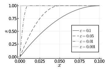
Figure 9. Plot of the smoothing function $s=s(x;\epsilon)$ for different values of $\epsilon$. It is used in (39) through (37) to approximate the Coulomb friction force.

To express the friction force as a function of all degrees of freedom, we first need to define the non-linearity above for all stacked tangential contact velocities $\bar{{\bf v}}\in\mathbb{R}^{2n_{c}}$:

$${\boldsymbol{\eta}}(\bar{{\bf v}})\equiv(\tilde{\boldsymbol{\eta}}(\bar{{\bf v}}_{1}),\tilde{\boldsymbol{\eta}}(\bar{{\bf v}}_{2}),\dots,\tilde{\boldsymbol{\eta}}(\bar{{\bf v}}_{n}))\in\mathbb{R}^{2n_{c}}.$$ (38)

For convenience let us define the diagonal matrix

$$\Lambda={\rm diag}[\lambda_{1},\lambda_{1},\lambda_{2},\lambda_{2},\ldots,\lambda_{n},\lambda_{n}].$$

Then the total friction force can be written compactly as

$${\bf f}_{\mathrm{f}}({\bf q},{\bf v})\equiv-\mu T({\bf q})\Lambda({\bf q}){\boldsymbol{\eta}}\left(T({\bf q})^{\top}{\bf v}\right).$$ (39)

Like with contact, the friction formulation here can deviate from traditional models, as allowed by the limited simulation durations that arise in computer animation. This formulation deviates from [30] since here we are not compelled to minimize an incremental potential. Instead we opt to solve a single system of non-linear equations. We hope that this simple view of an otherwise complex problem is more accessible and can motivate novel efficient numerical methods with supporting analyses in future work.

Above we have described a situation where discontinuities arise from an interface of codimension 1. Cases with higher codimension can be handled in the same way upon viewing these objects as having some thickness, which is consistent with the assumption that contacting objects are allowed to rest at some distance apart. We refer the reader to [31] for a more thorough analysis of additional difficulties encountered when simulating codimensional objects.

5.3. Combining the forces

Putting together all forces for the equations of motion in (3) we get

$$\dot{{\bf q}} ={\bf v},$$

$$M\dot{{\bf v}} =-\frac{\partial W}{\partial{\bf q}}({\bf q})$$ (elasticity)

$$-D({\bf q}){\bf v}$$ (damping)

$$+{\boldsymbol{\lambda}}({\bf q})^{\top}\frac{\partial{\bf d}}{\partial{\bf q}}({\bf q})$$ (contact)

$$-\mu T({\bf q})\Lambda({\bf q}){\boldsymbol{\eta}}\left(T({\bf q})^{\top}{\bf v}\right)$$ (friction)

$$+{\bf f}_{\mathrm{ext}}.$$ (external forces)

The complexity of these equations gives rise to a plethora of potentially useful integration schemes as discussed in previous sections. However, even the simplest integrators face challenges, since the friction term is often difficult to differentiate. It has long been known [18] that there is no single energy potential to derive these equations. Nevertheless, a number of works in computer graphics have been able to incorporate friction into a variational context [26, 30, 28].

6. Conclusion

The task of animating flexible objects efficiently and reliably has many practical applications, yet it can be rather challenging. Many physics-based approaches have been considered in the past few decades, and more are sure to appear. To more fully appreciate such efforts it is important to view resulting animation videos, not only formulas. Fortunately, just about any paper in this area in recent years comes supplemented with such a video demonstration, and the reader is thus urged to check them out. This area is teeming with opportunities for applied and numerical mathematics research.

In this paper we have concentrated on the constrained, potentially very large dynamical system of differential equations that results from an FEM discretization in space. Aspects of numerical methods for large systems of ODEs immediately arise, and the long Section 3 is devoted to this. Our new contribution here is the investigation of two popular DIRK methods, (8) and (9), which have been found to perform generally similarly with the exception that SDIRK can be potentially more efficient. See in particular the new damping curves in Figure 3. Further quests into improving performance and utility using additive ODE methods have resulted in a model reduction scheme. This gives rise, in particular, to the exciting possibility of using semi-implicit methods effectively, which eliminates the need for solving difficult nonlinear algebraic equations. In Section 5, upon considering methods for handling contact and friction, we encounter large systems of ODEs with algebraic inequality constraints, and these are handled by barrier methods that hail from the numerical optimization field.

In the same breath, it is imperative for numerical and applied mathematicians to keep in mind, as already mentioned in this paper’s abstract, that the “rules of the game” are different here than in usual numerical analysis.

• The mathematical model is not fully given, and it may well be adjusted in order to produce desired results. This implies, in particular, that the usual numerical analysis notion of comparing accuracy among methods is less relevant: it is the “eye norm” that rules here.

• Geometric numerical integration methods are relatively scarce in this field even though the ODE problems in (1) and (3) look on a casual glance to be ripe for such a treatment.

• The recent decisive employment of barrier penalty functions in Section 5 stems from the realization that, in the present context, smoothness of the model is very important. (NB The usual treatment of friction, in both graphics and engineering, previously considered it a non-smooth problem.) Thus, the temptation to get closer to the exact non-smooth constraint can be harmful in these contexts. In other words, it’s not merely a question of ill-conditioning or of computational cost, as in the optimization literature.

• Special FEM techniques had to be tailored for the animation applications under consideration.

There are several other aspects of the class of applications considered here that we have barely touched upon in our attempt to stay focussed, and which require additional expertise from new and traditional numerical and applied mathematics. These include inverse problems, homogenization, various learning techniques, variational methods and FEM, and much more.

References

- [1] Awad H Al-Mohy and Nicholas J Higham. Computing the action of the matrix exponential, with an application to exponential integrators. SIAM journal on scientific computing, 33(2):488–511, 2011.
- [2] R. Alexander. Diagonally implicit runge-kutta methods for stiff ode’s. SIAM J. Numer. Anal., 14(6):1006–1021, 1977.
- [3] U. Ascher. Numerical Methods for Evolutionary Differential Equations. SIAM, Philadelphia, PA, 2008.
- [4] U. Ascher and L. Petzold. Computer Methods for Ordinary Differential Equations and Differential-Algebraic Equations. SIAM, Philadelphia, PA, 1998.
- [5] J Awrejcewicz, D Grzelczyk, and Yu Pyryev. 404. a novel dry friction modeling and its impact on differential equations computation and lyapunov exponents estimation. Journal of Vibroengineering, 10(4), 2008.
- [6] David Baraff and Andrew Witkin. Large steps in cloth simulation. In Proceedings of the 25th annual conference on Computer graphics and interactive techniques, pages 43–54. ACM, 1998.
- [7] Jernej Barbic and Doug James. Real-time subspace integration for st. venant-kirchhoff deformable models. ACM Trans. Graphics, 24(4):982–990, 2005.
- [8] Eddy Boxerman and Uri Ascher. Decomposing cloth. In Proceedings of the 2004 ACM SIGGRAPH/Eurographics symposium on Computer animation, pages 153–161. Eurographics Association, 2004.
- [9] J.C. Butcher and D.J.L. Chen. A new type of singly-implicit runge-kutta method. Applied Numerical Mathematics, 34:179–188, 2000.
- [10] Desai Chen, David I. W. Levin, Wojciech Matusik, and Danny M. Kaufman. Dynamics-aware numerical coarsening for fabrication design. ACM Trans. Graph., 36(4):84:1–84:15, July 2017.
- [11] Yu Ju Chen, Uri Ascher, and Dinesh K Pai. Exponential rosenbrock-euler integrators for elastodynamic simulation. IEEE Transactions on Visualization and Computer Graphics, 24(10):2702–2713, 2018.
- [12] Yu Ju (Edwin) Chen, David I. W. Levin, Danny M. Kaufman, Uri M. Ascher, and Dinesh K. Pai. Eigenfit for consistent elastodynamic simulation across mesh resolution. Proceedings SCA, 2019. doi.org/10.1145/3309486.3340248.
- [13] Yu Ju (Edwin) Chen, Seung Heon Sheen, Uri M. Ascher, and Dinesh K. Pai. Siere: a hybrid semi-implicit exponential integrator for efficiently simulating stiff deformable objects. ACM Transactions on Graphics (TOG), 40(1):1–12, 2020.
- [14] J. Chung and G.M. Hulbert. A time integration algorithm for structural dynamics with improved numerical dissipation: the generalized- method. J. Applied Mech., 60:371–375, 1993.
- [15] Jintai Chung and GM Hulbert. A time integration algorithm for structural dynamics with improved numerical dissipation: the generalized- method. Journal of applied mechanics, 60(2):371–375, 1993.
- [16] Philippe G Ciarlet. Three-dimensional elasticity, volume 20. Elsevier, 1988.
- [17] Gilles Daviet, Florence Bertails-Descoubes, and Laurence Boissieux. A hybrid iterative solver for robustly capturing coulomb friction in hair dynamics. ACM Trans. Graph., 30(6):1–12, December 2011.
- [18] G. De Saxcé and Z. Q. Feng. The bipotential method: A constructive approach to design the complete contact law with friction and improved numerical algorithms. Mathematical and Computer Modelling, 28(4):225–245, August 1998.
- [19] Kenny Erleben. Rigid body contact problems using proximal operators. In Proceedings of the ACM SIGGRAPH / Eurographics Symposium on Computer Animation, SCA ’17, pages 13:1–13:12, New York, NY, USA, 2017. ACM.
- [20] Zachary Ferguson, Minchen Li, Teseo Schneider, Francisca Gil-Ureta, Timothy Langlois, Chenfanfu Jiang, Denis Zorin, Danny M. Kaufman, and Daniele Panozzo. Intersection-free rigid body dynamics. ACM Transactions on Graphics (SIGGRAPH), 40(4), 2021.
- [21] Theodore F. Gast, Craig Schroeder, Alexei Stomakhin, Chenfantu Jiang, and Joseph J. Teran. Optimization integrator for large time steps. IEEE Trans Visualization and Computer Graphics, 21(10):1103–1115, 2015.
- [22] Moritz Geilinger, David Hahn, Jonas Zehnder, Moritz Bacher, Bernhard Thomaszewski, and Stelian Coros. Add: Analytically differentiable dynamics for multi-body systems with frictional contact. ACM Transactions on Graphics (TOG), 39(6), 2020.
- [23] E. Hairer, C. Lubich, and G. Wanner. Geometric Numerical Integration. Springer, 2002.
- [24] E. Hairer and G. Wanner. Solving Ordinary Differential Equations II: Stiff and Differential-Algebraic Problems. Springer, 1996. 2nd Edition.
- [25] C. Kane, J. Marsden, M. Ortiz, and M. West. Variational integrators and the newmark algorithm for conservative and dissipative mechanical systems. Int. J. Numer. Meth. Eng., 49(10):1295–1325, 2000.
- [26] Danny M. Kaufman, Shinjiro Sueda, Doug L. James, and Dinesh K. Pai. Staggered projections for frictional contact in multibody systems. ACM Transactions on Graphics (SIGGRAPH Asia 2008), 27(5):164:1–164:11, 2008.
- [27] R. Kikuuwe, N. Takesue, A. Sano, H. Mochiyama, and H. Fujimoto. Fixed-step friction simulation: from classical Coulomb model to modern continuous models. In 2005 IEEE/RSJ International Conference on Intelligent Robots and Systems, pages 1009–1016, Edmonton, Alta., Canada, 2005. IEEE.
- [28] Egor Larionov, Ye Fan, and Dinesh K Pai. Frictional Contact on Smooth Elastic Solids. to appear in Transactions on Graphics, 2021.
- [29] R. J. LeVeque. Finite Difference Methods for Ordinary and Partial Differential Equations. SIAM, 2007.
- [30] Minchen Li, Zachary Ferguson, Timothy Langlois, Denis Zorin, Daniele Panozzo, Chenfanfu Jiang, and Danny M. Kaufman. Incremental potential contact: Intersection- and inversion-free, large-deformation dynamics. ACM Transactions on Graphics (TOG), 39(4), 2020.
- [31] Minchen Li, Danny M. Kaufman, and Chenfanfu Jiang. Codimensional Incremental Potential Contact. arXiv:2012.04457 [cs], January 2021. arXiv: 2012.04457.
- [32] Andreas Longva, Fabian Löschner, Tassilo Kugelstadt, José Antonio Fernández-Fernández, and Jan Bender. Higher-order finite elements for embedded simulation. ACM Transactions on Graphics, 39(6):1–14, November 2020.
- [33] Fabian Loschner, Andreas Longva, Stefan Jeske, Tassilo Kugelstadt, and Jan Bender. Higher order time integration for deformable solids. Computer Graphics Forum, 39(8):157–169, December 2020.
- [34] Per Lotstedt. Mechanical systems of rigid bodies subject to unilateral constraints. SIAM J. Appl. Math., 42:281–296, 1982.
- [35] Per Lotstedt and Linda Petzold. Numerical solution of nonlinear differential equations with algebraic constraints i: Convergence results for backward differentiation formulas. Math. Comp., 46:491–516, 1986.
- [36] Dominik L Michels, Vu Thai Luan, and Mayya Tokman. A stiffly accurate integrator for elastodynamic problems. ACM Transactions on Graphics (TOG), 36(4):116, 2017.
- [37] Dominik L. Michels and J. Paul T. Mueller. Discrete computational mechanics for stiff phenomena. In SIGGRAPH ASIA 2016 Courses, pages 13:1–13:9. ACM, 2016.
- [38] Cleve Moler and Charles Van Loan. Nineteen dubious ways to compute the exponential of a matrix, twenty-five years later. SIAM Rev., 45(1):3–49, 2003.
- [39] Jitse Niesen and Will M. Wright. Algorithm 919: A Krylov subspace algorithm for evaluating the -functions appearing in exponential integrators. ACM Trans. Math. Software (TOMS), 38(3):article 22, 2012.
- [40] J. Nocedal and S. Wright. Numerical Optimization. New York: Springer, 1999.
- [41] D. K. Pai, K. van den Doel, D. L. James, J. Lang, J. E. Lloyd, J. L. Richmond, and S. H. Yau. Scanning physical interaction behavior of 3D objects. In Computer Graphics (ACM SIGGRAPH 2001 Conference Proceedings), pages 87–96, August 2001.
- [42] Dinesh K Pai, Austin Rothwell, Pearson Wyder-Hodge, Alistair Wick, Ye Fan, Egor Larionov, Darcy Harrison, Debanga Raj Neog, and Cole Shing. The human touch: measuring contact with real human soft tissues. ACM Transactions on Graphics (TOG), 37(4):58, 2018.
- [43] Eftychios Sifakis and Jernej Barbic. FEM simulation of 3D deformable solids: a practitioner’s guide to theory, discretization and model reduction. In ACM SIGGRAPH 2012 Courses, page 20. ACM, 2012.
- [44] Breannan Smith, Fernando de Goes, and Theodore Kim. Stable neo-hookean flesh simulation. ACM Trans. Graph., December 2017.
- [45] Olga Sorkine and Marc Alexa. As-rigid-as-possible surface modeling. Eurographics Symposium on Geometry Processing, 4:109–116, 2007.
- [46] Mickeal Verschoor and Andrei C. Jalba. Efficient and accurate collision response for elastically deformable models. ACM Trans. Graph., 38(2), March 2019.
- [47] B. Wang, L. Wu, K. Yin, U. Ascher, L. Liu, and H. Huang. Deformation capture and modelling of soft objects. ACM trans. on Graphics (SIGGRAPH), 34(3), 2015.
- [48] Jerzy Wojewoda, Andrzej Stefański, Marian Wiercigroch, and Tomasz Kapitaniak. Hysteretic effects of dry friction: modelling and experimental studies. Philosophical Transactions of the Royal Society A: Mathematical, Physical and Engineering Sciences, 366(1866):747–765, March 2008.
- [49] H. Xu and J. Barbic. Example-based damping design. ACM Trans. Graphics, 36(4), 2017.