Abstract

While the need for interpretable machine learning has been established, many common approaches are slow, lack fidelity, or hard to evaluate. Amortized explanation methods reduce the cost of providing interpretations by learning a global selector model that returns feature importances for a single instance of data. The selector model is trained to optimize the fidelity of the interpretations, as evaluated by a predictor model for the target. Popular methods learn the selector and predictor model in concert, which we show allows predictions to be encoded within interpretations. We introduce EVAL-X as a method to quantitatively evaluate interpretations and REAL-x as an amortized explanation method, which learn a predictor model that approximates the true data generating distribution given any subset of the input. We show EVAL-X can detect when predictions are encoded in interpretations and show the advantages of REAL-x through quantitative and radiologist evaluation.

1 INTRODUCTION

The spread of machine learning models within many crucial aspects of society, has made interpretable machine learning increasingly consequential for trusting model decisions (Lipton,, 2017), identifying model failure modes (Zech et al.,, 2018), and expanding knowledge (Silver et al.,, 2017). Interpretability in machine learning is a well-studied problem, and many methods have been introduced to offer an understanding of which features locally, in a given instance of data, are important for generating the target. This goal can be stated as instance-wise feature selection (iwfs). For example, iwfs produces saliency maps to explains images, where pixels are segmented based on their importance.

Providing interpretable explanations is a difficult problem, and many popular approaches are either slow or lack fidelity and are hard to evaluate. Locally-linear methods (Lundberg and Lee,, 2017; Ribeiro et al.,, 2016) and perturbation methods (Zeiler and Fergus,, 2014) are slow — relying on evaluating numerous feature subsets or solving an optimization problem for each instance of data. While gradient-based methods (Simonyan et al.,, 2013; Springenberg et al.,, 2014) provide faster explanations, recent studies (Adebayo et al.,, 2018; Hooker et al.,, 2019) have shown that their explanations are inaccurate/lack fidelity.

Recently, multiple works (Dabkowski and Gal,, 2017; Chen et al.,, 2018; Yoon et al.,, 2019; Schwab and Karlen,, 2019), which we refer to as amortized explanation methods (AEMs), amortize the cost of providing model-agnostic explanations by learning a single global selector model that efficiently identifies the subset of locally important features in an instance of data with a single forward pass. AEMs learn the global selector model by optimizing an objective that measures the fidelity of the explanations.

AEMs assess feature subset selections, provided as masked inputs, using a predictor model for the target. Either the original predictor model trained on the full feature set is used or a new predictor model is trained. If the original predictor model is used and simple masking, such as with a default value, is employed, (Dabkowski and Gal,, 2017; Schwab and Karlen,, 2019) the masked inputs will come from a different distribution than that on which the model was trained, violating a key assumption in machine learning (Hooker et al.,, 2019). Instead, L2X and invase fit a new predictor model jointly with the selector model. We refer to such methods as joint amortized explanation methods (JAMs). JAMs have been used for a range of applications — providing image saliency maps, identifying important sentences in text, and identifying features involved in predicting mortality at the patient-level (Chen et al.,, 2018; Yoon et al.,, 2019).

While JAMs seek to provide users with fast, high fidelity explanations, we show that they encode predictions within interpretations and omit features involved in control flow.

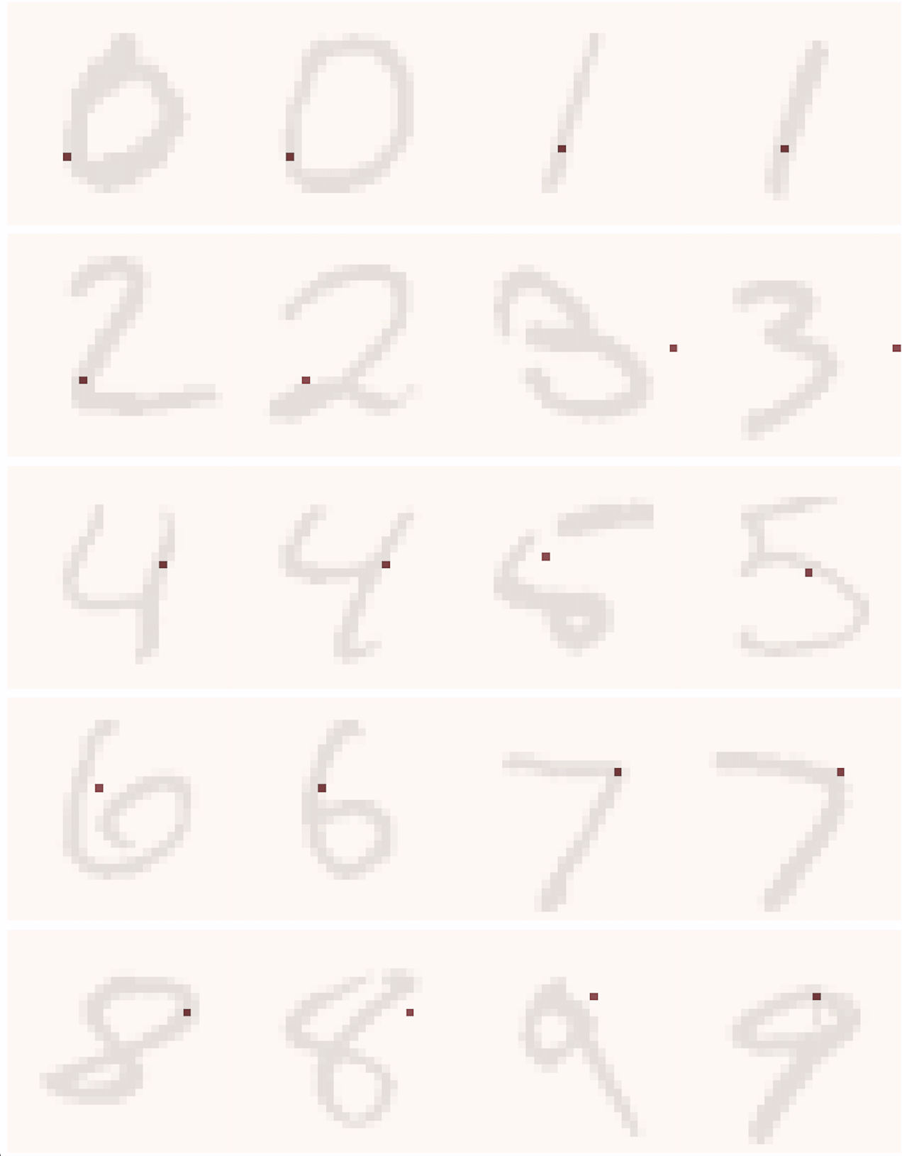
Figure 1: L2X classifies digits with $96\%$ accuracy from a single feature selection.

Figure 1 illustrates this point; it plots explanations from L2X Chen et al., (2018) on MNIST (LeCun et al.,, 1998) trained with a selector model that outputs a single important pixel and achieves 96.0% accuracy. Here, the selector model makes the classification decision and transmits it to the predictor model via the binary code of the selections, encoding the prediction. The issues with JAMs stem from the predictor model co-adapting to work with the selector model to fit the data, allowing the predictor model to map from selection masks to predictions. Had the selections in fig. 1 been evaluated under the true data generating distribution of the target given single feature subsets of the input, the digits could not have been accurately predicted. To identify such issues in practice, interpretations should be evaluated.

We first develop EVAL-X as a method to evaluate interpretations, which learns to approximate the true data generating distribution of the target given subsets of the input. Then, we introduce REAL-x as a novel AEM, which learns to select minimal feature subsets that maximize the likelihood of the data under an estimate of the true data generating distribution of the target given subsets of the input. REAL-x provides fast, high fidelity/accuracy explanations without encoding predictions or relying on model predictions generated by out-of-distribution inputs. We compare REAL-x to existing JAMs on established synthetic, MNIST, and Chest X-Ray datasets. We show that REAL-x helps address the issues with JAMs through quantitative EVAL-X and expert clinical evaluation.

1.1 Related Work

Interpretability methods can be divided into four different approaches – gradient-based, perturbation-based, locally linear, and amortized explanation methods.

Gradient-based methods, such as (Simonyan et al.,, 2013; Springenberg et al.,, 2014; Shrikumar et al.,, 2017), calculate the gradient of the target with respect to features in the input. Simonyan et al., (2013), for example, does so with imaging data, overlaying a "saliency map" of important pixels. Similarly, grad-CAM (Selvaraju et al.,, 2019) calculates the gradient of the target with respect to intermediate layers in a CNN. In addition to often requiring strong modeling assumptions (i.e. restricting the model class to CNNs), these methods do not optimize any objective to ensure the fidelity/accuracy of their explanations. Hooker et al., (2019) show that the estimates of feature importance derived from many gradient-based methods are often no better than a random assignment of feature importance. Adebayo et al., (2018) show that even random model parameters and targets provide seemingly acceptable explanations.

Perturbation-based approaches, such as (Zeiler and Fergus,, 2014; Zhou and Troyanskaya,, 2015; Zintgraf et al.,, 2017), perturb the inputs and observe the effect on the target or neurons within a network in order to gauge feature importance. This process requires separate forward passes through the network for each perturbation, which is computationally inefficient and can underestimate the importance of features (Shrikumar et al.,, 2017).

Locally linear methods, popularly lime (Ribeiro et al.,, 2016) and shap (Lundberg and Lee,, 2017), provide an explanation that is a linear function of simplified variables to explain the prediction of a single input. Locally linear methods assume model linearity in order to explain complex feature interactions and non-linear decision boundaries. These methods require selecting different feature subsets for each instance in order to assess the their impact on the prediction of the target, a computationally-intensive process. In order to assess model predictions given only a subset of features, the missing features are sampled independently, resulting in model inputs that can be out-of-distribution. This can lead to unexpected results because there is no expectation on what the model will return on out-of-distribution inputs. While these methods do optimize for the fidelity of their explanations, they are slow, require strong modeling assumptions, such as linearity, and rely on out-of-distribution estimates.

Amortized explanation methods, (Dabkowski and Gal,, 2017; Chen et al.,, 2018; Yoon et al.,, 2019; Schwab and Karlen,, 2019), learn a global model to explain any sample of data. AEMs are the only class of methods that provide both an objective to measure explanation fidelity and fast explanations with a single forward pass. AEMs accomplish all this while only requiring that the predictor model is differentiable, demanding no strong modeling assumptions. However, current approaches either rely on out-of-distribution model inputs (Dabkowski and Gal,, 2017; Schwab and Karlen,, 2019) or, as we show, encode predictions (Chen et al.,, 2018; Yoon et al.,, 2019). We address these issues with REAL-x.

Meanwhile, evaluating interpretations is less well studied. Given the interpretations, many approaches mask out the unimportant features in the inputs and assess their ability to predict the target. Most approaches (Samek et al.,, 2017; Chen et al.,, 2018) do so using a prediction model trained on the full feature set. In this case, the masked inputs come from a different distribution than those on which the model is trained. To address this issue, Hooker et al., (2019) introduced ROAR, which instead retrains a prediction model on the masked-inputs. However, if the predictions are encoded within the interpretations, then ROAR can learn these encodings. We introduce EVAL-X to address these issues.

2 AMORTIZED EXPLANATIONS

We begin by introducing some preliminaries that we refer to throughout the paper. Let features ${\mathbf{x}}$ be a random vector in $\mathbb{R}^{D}$, and the response ${\mathbf{y}}\in\{1,\dots,K\}$. For a given positive integer $j\leq D$, let ${\mathbf{x}}_{j}$ be the $j$th component of ${\mathbf{x}}$ and ${\mathbf{x}}_{\mathcal{S}}:=\{{\mathbf{x}}_{j}\}_{j\in\mathcal{S}}$ be a subset of features, where $\mathcal{S}\subseteq\{1,\dots,D\}$. $F$ is a distribution over $({\mathbf{x}},{\mathbf{y}})$.

For every instance $({\bm{x}}^{(i)},{\bm{y}}^{(i)})\sim F({\mathbf{x}},{\mathbf{y}})$, instance-wise feature selection (iwfs) identifies a minimal subset of features ${\bm{x}}^{(i)}_{\mathcal{S}^{(i)}}$ that are relevant to the corresponding target ${\bm{y}}^{(i)}$, Formally, iwfs seeks ${\bm{x}}^{(i)}_{\mathcal{S}^{(i)}}$ such that under the conditional distribution $F({\mathbf{y}}\mid\cdot)$ (Yoon et al.,, 2019)

$$F({\mathbf{y}}\mid{\mathbf{x}}_{\mathcal{S}^{(i)}}={\bm{x}}_{\mathcal{S}^{(i)}}^{(i)})=F({\mathbf{y}}\mid{\mathbf{x}}={\bm{x}}^{(i)}).$$ (1)

Here, $F({\mathbf{y}}\,|\,{\mathbf{x}})$ can either be the population distribution from which the data is drawn or, to provide model interpretations, a trained model.

2.1 Amortized Explanation Methods (AEMs)

AEMs refer to a general class of interpretability methods that learn a global selector model to identify a subset of important features locally in any given instance of data $({\bm{x}}^{(i)},{\bm{y}}^{(i)})$. The selector model is a distribution $q_{\text{sel}}({\mathbf{s}}\,|\,{\mathbf{x}};\beta)$ over a selector variable ${\mathbf{s}}$, which indicates the important features for a given sample of ${\mathbf{x}}$. For images, the selector model returns the salient pixels. AEMs optimize $q_{\text{sel}}$ with an objective that measures the fidelity of the selections (i.e. the ability of the selections to predict the target).

Joint amortized explanation methods (JAMs).

Recent, popular AEMs, L2X (Chen et al.,, 2018) and invase (Yoon et al.,, 2019) learn $q_{\text{sel}}({\mathbf{s}}\,|\,{\mathbf{x}};\beta)$ in concert with a predictor model $q_{\text{pred}}({\mathbf{y}}\,|\,m({\mathbf{x}},{\mathbf{s}});\theta)$. We refer to such methods as joint amortized explanation methods (JAMs). JAMs use a regularizer $R({\mathbf{s}})$ to control the number of selected features and a masking function $m$ to hide the $j$th feature ${\bm{x}}_{j}$ with the selector variable ${\bm{s}}_{j}$. For example, the masking function $m$ can replace features with a mask token mask using binary indicators ${\bm{s}}$:

$$m({{\bm{x}}}^{(i)},{{\bm{s}}}^{(i)})_{j}=\begin{cases}{{\bm{x}}}^{(i)}_{j}&\text{ if }{{\bm{s}}}^{(i)}_{j}=1\\ [\texttt{mask}]&\text{ if }{{\bm{s}}}^{(i)}_{j}=0\end{cases}.$$ (2)

To learn the parameters of the selector model, $\beta$, and the predictor model, $\theta$, the JAM objective maximizes

$$\mathbb{E}_{{\bm{x}},{\bm{y}}\sim F}\mathbb{E}_{{\bm{s}}\sim q_{\text{sel}}({\mathbf{s}}\,|\,{\bm{x}};\beta)}\left[\log q_{\text{pred}}({\bm{y}}\mid m({\bm{x}},{\bm{s}});\theta)-\lambda R({\bm{s}})\right]$$ (3)

This objective seeks to measure the ability of the selections to predict the target. Equation 3 can be optimized with score function (Glynn,, 1990; Williams,, 1992) or reparameterization gradients (Kingma and Welling,, 2014) and doesn’t make any model-specific assumptions like linearity.

Invase is a JAM that models the selector variable ${\mathbf{s}}$ using independent Bernoulli distributions denoted $\mathcal{B}$ whose probabilities are given by a function $f$ of the features. It sets $R({\mathbf{s}})=\ell_{0}({\mathbf{s}})$ to enforce sparse feature selections and uses the masking from eq. 2. Invase also uses $q_{\text{control}}({\bm{y}}\mid{\bm{x}};\phi)$ as a control variate within the objective to reduce the variance of the score function gradients during optimization. The invase objective for learning $\theta$ and $\beta$ is

$$\mathbb{E}_{{\bm{x}},{\bm{y}}\sim F}\mathbb{E}_{{\bm{s}}_{j}\sim\mathcal{B}(f_{\beta}({\bm{x}})_{j})} \big{[}\log q_{\text{pred}}({\bm{y}}\mid m({\bm{x}},{\bm{s}});\theta)$$

$$-\log q_{\text{control}}({\bm{y}}\mid{\bm{x}};\phi)-\lambda\|{\mathbf{s}}\|_{0}\big{]}$$

The use of $q_{\text{control}}$ does not alter Invase’s objective with respect to the selector or predictor model, so it fits into the form of eq. 3.

L2X is a JAM that uses $k$ independent samples from a Concrete distribution (Maddison et al.,, 2016; Jang et al.,, 2017) to define the selector model in order to make use of reparameterization gradients during optimization. In L2X, ${\mathbf{s}}$ is sampled from $q_{\text{sel}}({\mathbf{s}}\,|\,{\bm{x}};\beta)$ as

$${\bm{c}}_{j}\sim\text{Concrete}(f_{\beta}({\bm{x}})),\quad C=\left[{\bm{c}}_{1},\dots,{\bm{c}}_{k}\right]\in\mathbb{R}^{D\times k},$$

$${\bm{s}}_{i}=\max_{1\leq j\leq k}C_{ij}$$

Selection with the mask function is accomplished with multiplication: $m({\mathbf{x}},{\mathbf{s}})={\mathbf{x}}\odot{\mathbf{s}}$. Sparse selections are enforced by selecting a selection limit $k$ that sets the number of samples taken from a Concrete distribution, assigning a hard bound on the number of features selected. L2X optimizes the following objective for learning $\theta$ and $\beta$:

$$\mathbb{E}_{{\bm{x}},{\bm{y}}\sim F}\mathbb{E}_{s\sim q_{\text{sel}}({\mathbf{s}}\,|\,{\bm{x}};\beta)}\left[\log q_{\text{pred}}({\bm{y}}\mid{\bm{x}}\odot{\bm{s}};\theta)\right].$$ (4)

Equation 3 and eq. 4 represent the same constrained optimization problem, where in eq. 4 the constraint over the number of features selected is applied explicitly via the selection limit $k$.

3 PROBLEMS WITH JAMs

By maximizing an objective for providing high-fidelity selections, AEMs learn a selector model that makes it fast and simple to explain any new sample of data. In this section, however, we reveal a pair of problems with the JAM objective:

1. Encoding predictions with the learned selector.

2. Failure to select features involved in control flow.

3.1 Encoding Predictions

JAMs use the selector variable, ${\mathbf{s}}$, to make selections that mask features in the input. For simplicity, we focus on the masking function from eq. 2 and on independent Bernoulli selector variables ${\mathbf{s}}_{j}\sim\textrm{Bernoulli}(f_{\beta}({\mathbf{x}})_{j})$ like in Invase.

For noise free classification, the following lemma states that the selector model can encode the target using the selection of at most a single feature in each sample of data. The intuition here is that the selector variable ${\mathbf{s}}$ is a binary code that can pass quite a bit of information to predict the target. A proof is available in section D.1.

Lemma 1.

Let ${\mathbf{x}}\in\mathbb{R}^{D}$ and target ${\mathbf{y}}\in\{1,...,K\}$. If ${\mathbf{y}}$ is a deterministic function of ${\mathbf{x}}$ and $K\leq D$, then JAMs with monotone increasing regularizers $R$ will select at most one feature at optimality.

The proof for this lemma works by having the selector $q_{\text{sel}}$ make the classification based on its input ${\bm{x}}$, encode the class into a binary code, and transmit this code via the selector variable to $q_{\text{pred}}$ while making use of as few bits as possible. In this setting, if $K\leq D$, selection of only a single feature can encode the target. Further, if the regularizer $R$ is monotone increasing, then an encoding with a single feature will be the preferred maximizer of the JAM objective.

This idea can be generalized to settings where ${\mathbf{y}}$ is not a deterministic function of ${\mathbf{x}}$. In this case, levels of uncertainty can be encoded through the selected features. This is formally captured with lemma 3 in appendix C and proved in section D.2. Again, the intuition here is that selector variable produces many unique binary combinations. Each binary combination of the selector variable acts as an index that the predictor model uses to output a probability vector for the target classes. When the input dimensionality $D$ is large, a massive number of indices are available. This allows the selector model to accurately encode uncertainties about the target, without requiring that the predictor model use the input feature values.

3.2 Omitting Control Flow Features

default preamble= where n children=0 tier=word, diamond, aspect=2, , where level=0 if n=1 edge label=node[pos=.2, above] $\geq 0$, edge label=node[pos=.2, above] $<0$, , for tree= edge+=thick, -Latex, math content, s sep’+=1cm, draw, thick, edge path’= (!u) -| (.parent),

[x_11 [F_A(y|{x_i}_i=1^8) ] [F_B(y|{x_i}_i=4^10) ] ]

Figure 2: Generative process where the $F({\mathbf{y}}\mid{\mathbf{x}})$ is a tree.

Existing AEMs can learn to ignore features that only appear in the control flow of a generative process. We consider a simple example of such a process in fig. 2, where ${\mathbf{x}}_{i}\sim\mathcal{N}(0,1)$. Here, ${\mathbf{x}}_{11}$ is involved in a branching decision, such that based on its value either the subset of features ${\mathbf{x}}_{\mathcal{A}}=\{{\mathbf{x}}_{i}\}_{i=1}^{8}$ or ${\mathbf{x}}_{\mathcal{B}}=\{{\mathbf{x}}_{i}\}_{i=4}^{10}$ is used to generate ${\mathbf{y}}$. We refer to features, like ${\mathbf{x}}_{11}$, that are involved only in the branching decisions/nodes of tree structured generative process as control flow features.

Consider using a JAM to explain this process. In the first case, when ${\mathbf{x}}_{11}\geq 0$, the selector learns to select ${\mathbf{x}}_{\mathcal{A}}$, while the predictor model approximates $F_{A}$ to generate the target ${\mathbf{y}}$. Likewise, when ${\mathbf{x}}_{11}<0$ the selector can select ${\mathbf{x}}_{\mathcal{B}}$ and the predictor can generate ${\mathbf{y}}$ by modeling $F_{B}$. In all cases, the predictor model can use $F_{A}$ or $F_{B}$ based on the unique subset of features selected. JAMs do not select ${\mathbf{x}}_{11}$, even though ${\mathbf{x}}_{11}$ is important across all samples. Lemma 2 proved in section D.3 formalizes this phenomenon.

Lemma 2.

Assume that the true $F({\mathbf{y}}\mid{\mathbf{x}})$ is computed as a tree, where the leaves $\ell_{i}$ are the conditional distributions $F_{i}({\mathbf{y}}\mid{\mathbf{x}}_{\mathcal{S}_{i}})$ of ${\mathbf{y}}$ given distinct subsets of features $\mathcal{S}_{i}$ in ${\mathbf{x}}$. Given a monotone increasing regularizer $R$, the preferred maximizer of the JAM objective excludes control flow features that are involved in branching decisions.

The proof of this lemma works by having the selector select each distinct subset of features found at the leaves of the tree. Given that each distinct subset uniquely maps to an $F_{i}$, the predictor model can learn this mapping and generate the target as well as possible. Under monotone increasing regularization $R$, the solution that omits control flow features will be preferred over one that selects the full set of relevant features. While L2X does not employ monotone increasing regularization, the L2X objective still omits control flow features and encodes predictions when the selection limit $k$ is set appropriately to maximize the likelihood of the target while selecting the minimal number of features. Both L2X and invase benchmark their methods on datasets that contain control flow features. We describe these datasets and empirically demonstrate that JAMs fail to select control flow features in section 6.3.

Further, control flow features likely exist in many real-world datasets. Consider using electronic health record data to predict mortality in patients presenting with chest pain. Troponin lab values, a measure of heart injury, can function as a control flow feature. Abnormal Troponin values indicate that cardiac imagining should be used to assess disease severity and, therefore, mortality. Meanwhile, normal Troponin values indicate that the chest pain may be non-cardiac, and perhaps a chest X-Ray would better inform mortality prediction. In this case, using JAMs to interpret the prediction will not capture the roll that Troponin plays in determining a patient’s mortality.

4 EVAL-X: THE EVALUATOR

From the prior sections it is clear that JAMs can learn to make selections that, instead of selecting the set of relevant features, simply encode their contribution. In order to trust the explanations provided by JAMs, selections need to be quantitatively evaluated.

The goal of instance-wise feature selection (iwfs)is to find a minimal subset of features ${\bm{x}}^{(i)}_{\mathcal{S}^{(i)}}$ that are relevant to the corresponding target ${\bm{y}}^{(i)}$, which was stated in eq. 1 as

$$F({\mathbf{y}}\mid{\mathbf{x}}_{\mathcal{S}^{(i)}}={\bm{x}}_{\mathcal{S}^{(i)}}^{(i)})=F({\mathbf{y}}\mid{\mathbf{x}}={\bm{x}}^{(i)}).$$

The evaluation of iwfs should reflect the goal—the selections should be evaluated on the true conditional distribution $F({\mathbf{y}}\mid{\mathbf{x}}_{\mathcal{S}^{(i)}}={\bm{x}}_{\mathcal{S}^{(i)}}^{(i)})$. More generally, evaluating any potential selection of a subset of features $\mathcal{R}$ requires access to $F({\mathbf{y}}\mid{\mathbf{x}}_{\mathcal{R}}).$ We propose a new method for evaluating AEMs, called EVAL-X, which trains an evaluator model $q_{\text{eval-x}}$ to estimate this distribution by maximizing

$$\mathbb{E}_{{\bm{x}},{\bm{y}}\sim F}\mathbb{E}_{{\bm{r}}\sim\mathcal{B}(0.5)}\left[\log q_{\text{eval-x}}({\bm{y}}\,|\,m({\bm{x}},{\bm{r}});\eta)\right].$$ (5)

Here ${\mathbf{r}}$ is sampled randomly, independent of ${\mathbf{x}}$, from a Bernoulli distribution, mimicking any potential selection of the input. At optimality, EVAL-X learns the true $F({\mathbf{y}}\mid{\mathbf{x}}_{\mathcal{R}})$, which we show in appendix E. In practice, reaching optimality may be difficult. In section F.1 we compare the evaluations returned by EVAL-X against those returned by distinct models trained on each feature subset and show that EVAL-X performs similarly, where we consider the set of distinct models as ground truth. Algorithm 2 found in section B.1 summarizes the EVAL-X training procedure. In practice, predictive performance metrics returned by the EVAL-X should be used to quantitatively evaluate selections.

Of note, this evaluation differs from the common approach of simply masking the uninformative features and seeing how performance degrades on a model trained on the full feature set. Chen et al., (2018) suggests evaluating using post-hoc accuracy following this approach. However, as mentioned by Hooker et al., (2019), samples where a subset of the features are masked are out of the distribution of the original input. Hooker et al., (2019) address these out of distribution issues with ROAR, where they suggest training and testing a model on samples from the same distribution of masked inputs, $m({\mathbf{x}},{\mathbf{s}})$. However, this procedure allows the post-hoc evaluation model to learn the predictions encoded in the selector variable – precisely what should be avoided.

Evaluating explanations using EVAL-X not only aligns with the goal of instance-wise feature selection (iwfs), but also addresses the out of distribution issues.

5 REAL-X, LET US EXPLAIN!

We now describe our method to ensure that the learned selections also respect the true data distribution given subsets of the input $F({\mathbf{y}}\,|\,{\mathbf{x}}_{\mathcal{R}})$.

JAMs learn to select features and make predictions in concert. This flexibility allow JAMs to learn to make predictions from information encoded in the choice of selections. If the predictor model is learned disjointly, however, this possibility is eliminated.

Therefore, we propose learning the predictor model disjointly to approximate $F({\mathbf{y}}\,|\,{\mathbf{x}}_{\mathcal{R}})$ whilst learning to select the minimal subset of features to maximize the probability of the data. Given the insights of section 4, this procedure is expressed as learning $q_{\text{pred}}(\ \cdot\ ;\theta)$ to maximize

$$\mathbb{E}_{{\bm{x}},{\bm{y}}\sim F}\mathbb{E}_{{\bm{r}}\sim\mathcal{B}(0.5)}\left[\log q_{\text{pred}}({\bm{y}}\,|\,m({\bm{x}},{\bm{r}});\theta)\right],$$

while learning $q_{\text{sel}}(\ \cdot\ ;\beta)$ to maximize

$$\mathbb{E}_{{\bm{x}},{\bm{y}}\sim F}\mathbb{E}_{{\mathbf{s}}\sim q_{\text{sel}}({\mathbf{s}}\mid{\bm{x}};\beta)}\left[\log q_{\text{pred}}({\bm{y}}\mid m({\bm{x}},{\bm{s}});\theta)-\lambda R({\bm{s}})\right].$$

This modification to the training procedure ensures that $q_{\text{pred}}$ respects the true data distribution and avoids encoding predictions within the learned selector variable.

To make the method concrete, $q_{\text{sel}}$ and $R$ need to be chosen. We introduce the following procedure as REAL-x:

$$\max_{\beta}\mathbb{E}_{{\bm{x}},{\bm{y}}}\mathbb{E}_{{\mathbf{s}}_{i}\sim\mathcal{B}(f_{\beta}({\bm{x}})_{i})}\big{[}\log q_{\text{pred}}({\bm{y}}\mid m({\bm{x}},{\bm{s}});\theta)-\lambda\|{\bm{s}}\|_{0}\big{]},$$

$$\max_{\theta}\mathbb{E}_{{\bm{x}},{\bm{y}}}\mathbb{E}_{{\bm{r}}_{i}\sim\mathcal{B}(0.5)}\big{[}\log q_{\text{pred}}({\bm{y}}\mid m({\bm{x}},{\bm{r}});\theta)\big{]}.$$ (6)

REAL-x is a new AEM. REAL-x learns a global selector model to identify the subset of important features locally in any given instance of data. The selector model is trained on a global objective that measures selection fidelity. REAL-x uses discrete selections sampled independently from a Bernoulli distribution and penalizes the number of features selected.

5.1 Implementation

To optimize over discrete feature selections, REAL-x employs rebar gradients (Tucker et al.,, 2017), a score function gradient estimator that uses relaxed continuous selections within a control variate to lower the variance of the gradient estimates. Algorithm 1 summarizes the training procedure (reference appendix A for eqs. 8, 9, 10 and 11).

Algorithm 1 REAL-x Algorithm

Input: $\mathcal{D}:=({\bm{x}},{\bm{y}})$, where ${\bm{x}}\in\mathbb{R}^{N\times D}$, feature matrix; ${\bm{y}}\in\mathbb{R}^{N}$, labels

Output: $q_{\text{sel}}(\cdot;\beta)$, function that returns feature selections given an instance of ${\mathbf{x}}$

Select: $\lambda$, regularization constant; $\alpha$, learning rate; $M$, mini-batch size, $T$, training-steps

for $1,...,T$ do

       Randomly sample mini-batch of size $M$, $({{\bm{x}}}^{(i)},{{\bm{y}}}^{(i)})_{i=1}^{M}\sim\mathcal{D}$ for $i=1,...,M$ do

             Sample Selections:    ${{\bm{r}}}^{(i)}\sim\text{Bernoulli}(0.5)$    Sample ${{\bm{s}}}^{(i)}$, ${{\bm{z}}}^{(i)}$, and $\tilde{{\bm{z}}}^{(i)}$ using $q_{\text{sel}}(\cdot;\beta)$ as in                                           eqs. 8, 9 and 10

       end for

      Optimize Models:    $\theta=\theta+\alpha\nabla_{\theta}\left[\frac{1}{M}\sum_{i=1}^{M}\log q_{\text{pred}}({{\bm{y}}}^{(i)}|m({{\bm{x}}}^{(i)},{{\bm{r}}}^{(i)};\theta)\right]$    $\beta=\beta+\alpha\frac{1}{M}\sum_{i=1}^{M}\hat{g_{\beta}}$  ($\hat{g_{\beta}}$ as in eq. 11)

end for

Note that the user has the option to train $q_{\text{pred}}$ first, then optimize $q_{\text{sel}}$. We show in section F.2 that this approach performs similarly. The algorithm makes clear that the predictor model is updated independently of REAL-x’s learned selections and, therefore, cannot make accurate predictions from selections that directly encode the target or omit control flow features.

6 EXPERIMENTS

We have shown that existing AEMs can encode predictions within selections and fail to select features involved in control flow. We then introduced EVAL-X as a procedure for quantitatively evaluating explanations. Further, we proposed REAL-x as a simple method to address the issues with existing AEMs by mirroring our evaluation procedure.

In order to properly evaluate REAL-x, we introduce BASE-x as a baseline to ensure that the results we obtain on REAL-x are not due to changes in the optimization procedure. BASE-x is a JAM that mimics the gradient optimization and regularization procedure of REAL-x. We evaluate all the JAMs— L2X , invase , and BASE-x— and our method, REAL-x, on a number of established Synthetic Datasets, MNIST, and on real-world Chest X-Rays.

We show that REAL-x selects control flow features in synthetic data. On imaging data, we demonstrate that REAL-x obtains higher predictive performance on EVAL-X, while other method’s seek to encode the classification. Further, we elicit expert radiologist feedback to rank the explanations of cardiomegaly returned by each method.

6.1 Trading-Off Interpretability and Accuracy

While the goal of iwfs (eq. 1) assumes that a small human-interpretable subset of features generate the target, in practice there is a trade-off between interpretability and predictive accuracy. This trade-off has been discussed by many prior works (Selvaraju et al.,, 2019; Lakkaraju et al.,, 2017; Ishibuchi and Nojima,, 2007).

A simple explanation of the data, one with fewer features selected, allows for greater human interpretability. However, on real-word data this is likely to come at the cost of predictive accuracy. The AEMs considered optimize multiple objectives — an objective that measure the fidelity of the learned selections and an objective that measures the interpretability of the selections by limiting the number of features selected. By tuning the hyper-parameter balancing these objectives, different solutions along the multi-objective Pareto front can be reached to trade-off interpretability and predictive accuracy. For the real-world datasets, we, therefore, choose the hyper-parameter associated with the most interpretable solution such that the following condition is met: Accuracy (acc)is within $5$% of a model trained on the full feature set. We report the performance of the model trained on the full feature set, and refer to this model as FULL. For our synthetic datasets, we do not need to make this trade-off because we know that only a small number of interpretable features generate the target and instead chose the hyper-parameter that maximizes the accuracy.

6.2 Evaluation

We also evaluate the selections obtained by each method using the predictive performance measured by EVAL-X, which we denote as eauroc and eacc. Together, we show that good predictive performance, as measured by auroc and acc, attained by L2X and invase does not imply good performance upon evaluation with EVAL-X. A phenomenon that we have described explicitly in section 3. Whereas, REAL-x is more robust to these issues.

It is possible to use EVAL-X to select AEM models. However, for a JAM that at optimum encodes predictions or omits control flow features, the effectiveness of such a procedure would hinge on poor optimization of the JAM’s objective.

6.3 Synthetic Datasets

Both L2X and invase evaluate their methods on a number of synthetic datasets, where the data generation procedure is described as follows:

$${\{{\mathbf{x}}_{i}\}}_{i=1}^{11}\sim\mathcal{N}(0,1) \ \ \ \ \ \ \ {\mathbf{y}}\sim\text{Bernoulli}\left(\frac{1}{1+f({\mathbf{x}})}\right),$$

The functions for $f({\mathbf{x}})$ vary as follows:

• $f_{\textbf{A}}({\mathbf{x}})=$ exp(${\mathbf{x}}_{1}{\mathbf{x}}_{2}$)

• $f_{\textbf{B}}({\mathbf{x}})=$ exp($\sum_{i=3}^{6}{\mathbf{x}}_{i}^{2}-4$)

• $f_{\textbf{C}}({\mathbf{x}})=$ exp($-10\sin(0.2{\mathbf{x}}_{7})+|{\mathbf{x}}_{8}|+{\mathbf{x}}_{9}+e^{-{\mathbf{x}}_{10}}-2.4$),

resulting in the following datasets

• S1: If ${\mathbf{x}}_{11}<0$: $f_{\textbf{A}}({\mathbf{x}})$; else $f_{\textbf{B}}({\mathbf{x}})$

• S2: If ${\mathbf{x}}_{11}<0$: $f_{\textbf{A}}({\mathbf{x}})$; else $f_{\textbf{C}}({\mathbf{x}})$

• S3: If ${\mathbf{x}}_{11}<0$: $f_{\textbf{B}}({\mathbf{x}})$; else $f_{\textbf{C}}({\mathbf{x}})$

This data generating process contains a control flow feature. Let ${\mathbf{x}}_{\mathcal{A}}=\{{\mathbf{x}}_{i}\}_{i=1}^{2}$, ${\mathbf{x}}_{\mathcal{B}}=\{{\mathbf{x}}_{i}\}_{i=3}^{6}$, ${\mathbf{x}}_{\mathcal{C}}=\{{\mathbf{x}}_{i}\}_{i=7}^{10}$, and $F_{J}({\mathbf{y}}\,|\,{\mathbf{x}}):=\text{Bernoulli}\left(\frac{1}{1+f_{J}({\mathbf{x}})}\right)$ for some function $f_{J}$. $F({\mathbf{y}}\,|\,{\mathbf{x}})$ in S1-3 is computed as a tree, where ${\mathbf{x}}_{11}$ splits the data into the leaf conditional distributions $F_{A}({\mathbf{y}}\,|\,{\mathbf{x}}_{\mathcal{A}})$, $F_{B}({\mathbf{y}}\,|\,{\mathbf{x}}_{\mathcal{B}})$, or $F_{C}({\mathbf{y}}\,|\,{\mathbf{x}}_{\mathcal{C}})$. The feature sets ${\mathbf{x}}_{\mathcal{A}}$, ${\mathbf{x}}_{\mathcal{B}}$, and ${\mathbf{x}}_{\mathcal{C}}$ are distinct and do not contain ${\mathbf{x}}_{11}$. Thus, ${\mathbf{x}}_{11}$ is a control flow feature.

Model training.

The training and test sets both contained $10,000$ samples of data. For all methods, we used neural networks with $3$ hidden layers for the selector model and $2$ hidden layers for the predictor model. The hidden layers were linear with dimension 200. All methods were trained for $1,000$ epochs using Adam for optimization with a learning rate of $10^{-4}$. We tuned the hyper-parameters controlling the number of features to select across $k=\{1,2,3,4,5,6,7\}$ for L2X and $\lambda=\{0.05,0.075,.1,0.125,0.15,.2,.25\}$ for invase, REAL-x, and BASE-x. We select the configuration that yields the largest acc.

Table 1: REAL-x achieves superior CFSRs, TPRs, and post-hoc eauroc on instance-wise tasks.

Metric	Method	S1	S2	S3
CFSR	REAL-x	100.0	100.0	100.0
	L2X	24.3	31.2	61.5
	Invase	41.1	47.2	37.6
	BASE-x	35.0	24.5	27.2
TPR	REAL-x	98.4	96.7	93.5
	L2X	78.5	81.1	81.0
	Invase	80.6	80.4	86.3
	BASE-x	84.7	75.6	83.5
FDR	REAL-x	10.7	6.3	2.6
	L2X	22.0	20.2	19.0
	Invase	1.3	3.1	1.1
	BASE-x	1.3	1.6	1.1
AUROC	REAL-x	0.782	0.805	0.875
	L2X	0.752	0.790	0.852
	Invase	0.803	0.806	0.886
	BASE-x	0.799	0.805	0.886
eAUROC	REAL-x	0.774	0.804	0.873
	L2X	0.742	0.771	0.848
	Invase	0.740	0.783	0.868
	BASE-x	0.762	0.773	0.867
ACC	REAL-x	70.1%	71.5%	79.6%
	L2X	67.1%	70.5%	76.7%
	Invase	71.3%	71.4%	80.6%
	BASE-x	71.0%	71.2%	80.6%
eACC	REAL-x	68.6%	71.2%	79.3%
	L2X	68.4%	70.1%	76.9%
	Invase	66.8%	69.2%	78.8%
	BASE-x	68.5%	68.8%	78.7%
$k\text{ or }\lambda$	REAL-x	0.05	0.05	0.1
	L2X	4	4	5
	Invase	0.2	0.15	0.2
	BASE-x	0.15	0.125	0.2

Results.

We summarize our results for each dataset, paying special attention to the control flow feature selection rate (cfsr), defined by the proportion of control flow features selected. We also include the acc, auroc, the tpr, defined by the proportion of important features selected, the fdr, defined by the proportion of selected features that are not important, and the corresponding EVAL-X evaluation metrics (eauroc, eacc). We summarize these results in Table 1, which show that only REAL-x consistently selects the control flow feature and attains a higher tpr, eauroc, and eacc. From lemma 2 in section 3.2 we expect that JAMs should never select the control flow feature. However, the fact that JAMs occasionally do so is due to either incomplete optimization (invase) or no preference in selecting the control feature (L2X when $k$ is large enough). Yet, requiring REAL-x to predict well from random selections results in a slightly greater fdr. By not selecting control flow features, L2X and invase achieve lesser tprs. Though REAL-x often does not obtain the highest auroc and acc, it obtains greater eauroc and eacc upon evaluation with EVAL-X due to the selection of the control flow feature. These results help highlight REAL-x’s ability to address issues that prior methods have with selecting control flow features.

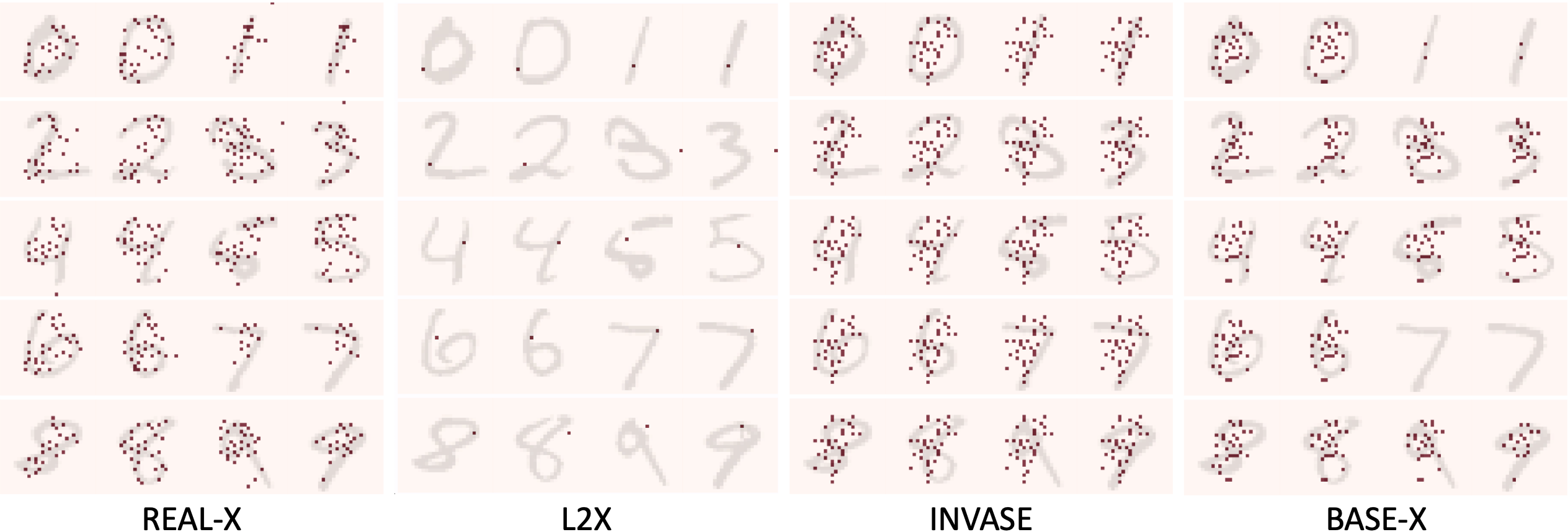
Figure 3: REAL-x makes reasonable selections, with other methods encode predictions. Each column is labeled with the method used to learn selections. For each digit two random samples are provided and selections are presented in dark red.

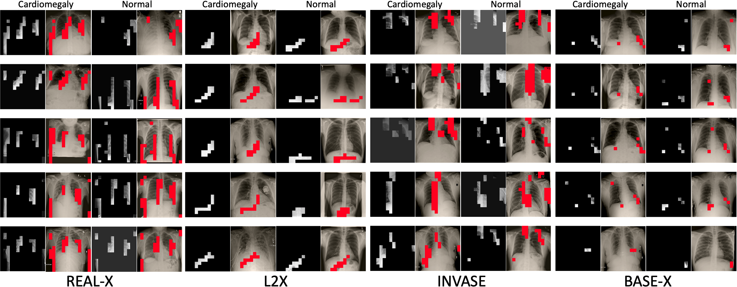
Figure 4: REAL-x makes reasonable selections around the margins of the heart without encoding the prediction. 5 random samples of Cardiomegaly and Normal Chest X-Rays are presented for each method. The selected inputs are places beside images with the selections overlaid in red.

6.4 MNIST

The MNIST dataset (LeCun et al.,, 1998) is comprised of $70,000$, $28\times 28$ images of handwritten digits in $\{0,...,9\}$.

Model training.

The images were trained using $60,000$ samples and evaluated on $10,000$ samples. For all methods, we used neural networks with $3$ hidden layers for the selector model and $2$ hidden layers for the predictor model. The hidden layers were linear with dimension 200. All methods were trained for $500$ epochs using Adam for optimization with a learning rate of $10^{-4}$. We tuned the hyper-parameters controlling the number of features to select across $k=\{1,5,15,50,100,200\}$ for L2X and $\lambda=\{0.1,1.0,5.0,10.0,25.0,50.0\}$ for invase, REAL-x, and BASE-x. We then selected the configuration that allowed for the smallest number of features to be selected while retaining an acc within $5$% of that obtained by a model trained on the full feature set.

Results.

Table 2: Digit pixels selected by REAL-x yield superior results upon post-hoc evaluation.

Method	acc	auroc	eacc	eauroc	$k\backslash\lambda$
FULL	97.8%	0.999	—	—	–
REAL-x	93.8%	0.997	86.7%	0.989	5.0
L2X	96.0%	0.998	11.4%	0.561	1
Invase	93.1%	0.996	50.3%	0.883	10.0
BASE-x	92.8%	0.996	56.9%	0.899	10.0

Table 2 shows that while L2X, invase, and BASE-x all make selections that allow for high predictive performance (acc $\geq 92.8\%$), when evaluated with EVAL-X the predictive performance is significantly worse. Looking at the selections made by each method on fig. 3 helps clarify this discrepancy. As we saw earlier, L2X can encode the prediction with a single feature. We also see evidence of encoding with BASE-x, where certain digits, $\{1,7\}$, are encoded by the selection of a few features or no features. Invase, however, seems to optimize poorly in high-dimensions and instead selects a conserved set of features across digits. REAL-x, however, performs far better upon EVAL-X evaluation. Also, REAL-x’s selections appear reasonable, selecting pixels along the entire digit or along regions that help distinguish digits.

6.5 Chest X-Ray Images

The NIH ChestX-ray8 Dataset (Wang et al.,, 2017) contains $112,120$ chest X-ray images from $30,805$ patients, each labeled with the presence of $8$ diseases. We selected a subset of $5,600$ X-rays labeled either cardiomegaly or normal, including all $2,776$ X-rays with cardiomegaly. Cardiomegaly is characterized by an enlarged heart, and can be diagnosed by measuring the maximal horizontal diameter of the heart relative to that of the chest cavity and assessing the contour of the heart. Given this, we expect to see selections that establish the margins of the heart and chest cavity.

Model training.

We used $5,000$, $300$, and $300$ images for training, validation, and testing respectively. UNet and DenseNet$121$ architectures were used for the selector and predictor models respectively. All methods were trained for $50$ epochs using a learning rate of $10^{-4}$. We choose to learn $16\times 16$ super-pixel selections. We tuned the hyper-parameters controlling the number of features to select across $k=\{1,5,15,50,100\}$ for L2X and $\lambda=\{0.1,1.0,2.5,5.0,50.0\}$ for invase, REAL-x, and BASE-x. We then selected the configuration that allowed for the smallest number of features to be selected while retaining an acc within $5$% of that obtained by a model trained on the full feature set.

Results.

Table 3: REAL-x yields superior post-hoc evaluation.

Method	acc	auroc	eacc	eauroc	$k\backslash\lambda$
FULL	78.0%	0.887	—	—	–
REAL-x	75.0%	0.838	70.3%	0.777	2.5
L2X	75.0%	0.848	54.0%	0.581	10
Invase	74.3%	0.819	52.3%	0.548	2.5
BASE-x	74.3%	0.818	51.7%	0.595	2.5

Table 3 shows that while each method makes selections that allow for high predictive performance (acc $\geq 73.0\%$), REAL-x yields superior performance upon EVAL-X evaluation. Looking at selections of random Chest X-rays in fig. 4, we see that L2X, BASE-x and invase seem to make counterintuitive selections that omit many of the important pixels, resulting in a sharp decline in eacc.

Physician Evaluation.

Table 4: Average rankings by expert radiologists.

REAL-x	L2X	Invase	BASE-x
1.08 (0.04)	3.57 (0.10)	2.85 (0.11)	2.29 (0.09)

We asked two expert radiologists to rank each method based on the explanations provided. We randomly selected $50$ Chest X-rays from the test set and displayed the selections made by each method for each X-ray in a random order to each radiologist. For a given Chest X-ray, the radiologists then evaluated which selections provided sufficient information to diagnose cardiomegaly and ranked the four options provided, allowing for ties. In table 4 we report the average rank each method achieved. We see that REAL-x consistently provides explanations that are meaningful to board-certified radiologists.

7 DISCUSSION

We proposed REAL-x, an AEM that provides interpretations that give high likelihood to the data efficiently with a single forward pass. Further, we introduced EVAL-X as a method to evaluate interpretations, detecting when predictions are encoded in explanations without making out-of-distribution queries of a model. EVAL-X produces an evaluator model to approximate the true data generating distribution given any subset of the input. One future direction could be to produce feature attributions, such as Shapley values, recognizing the evaluator model as a function on subsets for any data point.

With REAL-x, we employ amortization to provide fast interpretations. Amortization can help make many existing interpretation techniques scalable, though, as exemplified by JAMs, care must be taken to avoid encoding predictions within interpretations. For example, learning a locally linear model to explain each instance of data can be amortized by learning an global explanation model that takes an instance as input and outputs the parameters of a linear model that predicts the target for that instance. As with JAMs, the parameters outputted by the explanation model can be used to encode the target.

In addition to extending our methodology to allow for feature attributions, one can explore tailoring it for use with specific data modalities. For example, saliency maps are generally more human interpretable if the segmentation is smooth instead of disjoint pixel selections, as in fig. 3. We leave these avenues for future work.

Acknowledgements

We thank Dr. Lea Azour and Dr. William Moore for clinically evaluating each Chest X-ray explanation. We also thank the reviewers for their thoughtful feedback.

Neil Jethani was partially supported by NIH T32 GM136573. Mukund Sudarshan was partially supported by a PhRMA Foundation Predoctoral Fellowship. Yin Aphinyanaphongs was partially supported by NIH 3UL1TR001445-05 and National Science Foundation award #1928614. Mukund Sudarshan and Rajesh Ranganath were partly supported by NIH/NHLBI Award R01HL148248, and by NSF Award 1922658 NRT-HDR: FUTURE Foundations, Translation, and Responsibility for Data Science.

 

Supplementary Materials

 

Appendix A Applying REBAR Gradient Estimation to REAL-X

Computing the gradient of an expectation of a function with respect to the parameters of a discrete distribution requires calculating score function gradients. Score function gradients often have high variance. To reduce this variance, control variates are used within the objective. REBAR gradient calculation involves using a highly correlated control variate that approximates the discrete distribution with its continuous relaxation.

The REAL-x procedure involves

$$\max_{\beta}\mathbb{E}_{{\bm{x}},{\bm{y}}}\mathbb{E}_{{\mathbf{s}}_{i}\sim\mathcal{B}(f_{\beta}({\bm{x}})_{i})}\big{[}\log q_{\text{pred}}({\bm{y}}\mid m({\bm{x}},{\bm{s}});\theta)-\lambda\|{\bm{s}}\|_{0}\big{]}.$$

This is accomplished through stochastic gradient ascent by taking

$$\nabla_{\beta}\mathbb{E}_{{\mathbf{s}}_{i}\sim\mathcal{B}(f_{\beta}({\bm{x}})_{i})}\big{[}\log q_{\text{pred}}({\bm{y}}\mid m({\bm{x}},{\bm{s}});\theta)-\lambda\|{\bm{s}}\|_{0}\big{]},$$ (7)

which requires score function gradient estimation.

Let ${\mathbf{s}}$ be a discrete random variable, $\mathcal{L}=\mathbb{E}_{{\mathbf{s}}\sim q_{\beta}}[h({\mathbf{s}})]$, and $\mathbb{E}[\hat{g}_{\beta}]=\nabla_{\beta}\mathcal{L}$, the REBAR gradient estimator (Tucker et al.,, 2017) computes $\hat{g}_{\beta}$. Then, letting ${\mathbf{z}}$ be a continous relaxation of ${\mathbf{s}}$, REBAR estimates the gradient as

$$\hat{g}_{\beta}=[h({\bm{s}})-h(\tilde{{\bm{z}}})]\nabla_{\beta}\log q_{\beta}({\bm{s}})-\nabla_{\beta}h(\tilde{{\bm{z}}})+\nabla_{\beta}h({\bm{z}}),$$

$$\text{where}\quad{\bm{s}}=B({\bm{z}}),\ {\bm{z}}\sim q_{\beta}({\mathbf{z}}),\ \tilde{{\bm{z}}}\sim q_{\beta}({\mathbf{z}}|{\bm{s}}).$$

To estimate eq. 7 using REBAR, REAL-x sets

$$h({\bm{s}})=\log q_{\text{pred}}({\bm{y}}\mid m({\bm{x}},\ {\bm{s}}\ );\theta).$$

Here, ${\mathbf{s}}$ is Bernoulli distributed and REAL-x sets ${\mathbf{z}}$ to be distributed as the binary equivalent of the Concrete distribution (Maddison et al.,, 2016; Jang et al.,, 2017), which we refer to as the RelaxedBernoulli distribution. ${\mathbf{s}}$, ${\mathbf{z}}$, and $\tilde{{\mathbf{z}}}$ are sampled as described by Tucker et al., (2017) such that

$$p_{i}=f_{\beta}({\bm{x}})_{i},$$

$${\bm{s}}_{i}=B({\bm{z}}_{i})=\mathbbm{1}({\bm{z}}_{i}>0),$$ (8)

$${\bm{z}}_{i}\sim q_{\beta}({\mathbf{z}}\,|\,{\bm{x}})=\textit{RelaxedBernoulli}(p_{i};\tau=0.1),$$ (9)

$$\tilde{{\mathbf{z}}_{i}}\sim q_{\beta}({\mathbf{z}}\,|\,{\bm{x}},{\bm{s}})=\frac{1}{0.1}\left(\log\frac{p_{i}}{1-p_{i}}+\log\frac{{\bm{v}}^{\prime}}{1-{\bm{v}}^{\prime}}\right),$$ (10)

$$\text{ where }{\bm{v}}\sim\text{Unif}(0,1)\text{ and }{\bm{v}}^{\prime}=\begin{cases}{\mathbf{v}}(1-p_{i})&\text{if }{\bm{s}}_{i}=0\\ {\mathbf{v}}p_{i}+(1-p_{i})&\text{if }{\bm{s}}_{i}=1\end{cases}.$$

Then to estimate eq. 7 notice that

$$\nabla_{\beta}\mathbb{E}_{{\mathbf{s}}_{i}\sim\mathcal{B}(f_{\beta}({\bm{x}})_{i})}\big{[}\lambda\|{\bm{s}}\|_{0}\big{]}=\lambda\nabla_{\beta}f_{\beta}({\mathbf{x}}).$$

REAL-x, therefore, estimates eq. 7 by calculating $\hat{g}_{\beta}$ as

$$\hat{g}_{\beta}=\left[\log q_{\text{pred}}({\bm{y}}\mid m({\bm{x}},{\bm{s}}))-\log q_{\text{pred}}({\bm{y}}\mid m({\bm{x}},\tilde{{\bm{z}}}))\right]\nabla_{\beta}\log q_{\text{sel}}({\bm{s}}\,|\,{\bm{x}};\beta)-\lambda\nabla_{\beta}f_{\beta}({\bm{x}})$$

$$-\nabla_{\beta}q_{\text{pred}}({\bm{y}}\mid m({\bm{x}},\tilde{{\bm{z}}}))+\nabla_{\beta}q_{\text{pred}}({\bm{y}}\mid m({\bm{x}},{\bm{z}}))$$ (11)

Appendix B Algorithms

B.1 Evaluation Algorithm

Algorithm 2 Algorithm to Train Evaluator Model $q_{\text{eval-x}}$

Input: $\mathcal{D}:=({\bm{x}},{\bm{y}})$, where ${\bm{x}}\in\mathbb{R}^{N\times D}$, feature matrix; ${\bm{y}}\in\mathbb{R}^{N}$, labels

Output: $q_{\text{eval-x}}({\mathbf{y}}\,|\,m({\bm{x}},\ \cdot\ );\eta)$, function that returns the probability of the target given a subset of features.

Select: $\alpha$, learning rate; $M$, mini-batch size

while Converge do

       Randomly sample mini-batch of size $M$, $({{\bm{x}}}^{(i)},{{\bm{y}}}^{(i)})_{i=1}^{M}\sim\mathcal{D}$ for $i=1,...,M$ do

             Sample Selections:      ${{\bm{r}}}^{(i)}\sim\text{Bernoulli}(0.5)$

       end for

      Optimize:      $\eta=\eta+\alpha\nabla_{\eta}\left[\frac{1}{M}\sum_{i=1}^{M}\log q_{\text{eval-x}}({{\bm{y}}}^{(i)}|m({{\bm{x}}}^{(i)},{{\bm{r}}}^{(i)});\eta)\right]$

end while

Appendix C Lemmas

Lemma 3.

Let ${\mathbf{x}}\in\mathbb{R}^{D}$, target ${\mathbf{y}}\in\{1,...,K\}$, and $\Delta$ be a set of $K$ dimensional probability vectors, then for $J=\operatorname*{arg\,min}_{j}\sum_{i=0}^{j}\genfrac{(}{)}{0.0pt}{0}{D}{i}\geq|\Delta|$ and ${\mathbf{x}}\sim F$, there exists a $q_{\text{sel}}$ and $q_{\text{pred}}$, where $\{q_{\text{pred}}(y=k\,|\,m({\mathbf{x}},{\mathbf{s}}))\}_{k=1}^{K}=\delta({\mathbf{x}})\in\Delta$ and $E[||{\mathbf{s}}||_{0}]\leq J$.

Appendix D Proofs

D.1 Proof of Lemma 1

Lemma 1.

Let ${\mathbf{x}}\in\mathbb{R}^{D}$ and target ${\mathbf{y}}\in\{1,...,K\}$. If ${\mathbf{y}}$ is a deterministic function of ${\mathbf{x}}$ and $K\leq D$, then JAMs with monotone increase regularizers $R$ will select at most one feature at optimality.

As mentioning in section 3, the lemma considers the masking function from eq. 2 and on independent Bernoulli selector variables ${\mathbf{s}}_{j}\sim\textrm{Bernoulli}(f_{\beta}({\mathbf{x}})_{j})$.

${\mathbf{s}}\in\mathbb{R}^{D}$ is binary and, therefore, has the capacity to transmit D bits of information. Given that ${\mathbf{y}}\in\{1,...,K\}$ is a deterministic function of ${\mathbf{x}}\in\mathbb{R}^{D}$, the true distribution is $F({\mathbf{y}}\mid{\bm{x}})\in\{0,1\}$ for each of the $K$ realizations of ${\mathbf{y}}$. Therefore, $m({\bm{x}},{\bm{s}})$ must pass at least $\log_{2}{K}$ bits of information to the predictor model $q_{\text{pred}}({\mathbf{y}}\,|\,m({\bm{x}},{\bm{s}}))$.

With $m$ of the form eq. 2, this information content can come from ${\bm{s}}$. ${\bm{s}}$ has a capacity of $\log_{2}\left(\sum_{i=1}^{n}\genfrac{(}{)}{0.0pt}{0}{D}{i}\right)$ bits when restricted to realizations of ${\bm{s}}\sim q_{\text{sel}}$ with at most $n$ non-zero elements. The maximal number of non-zero elements $J$ in any given realization of ${\mathbf{s}}$ required to minimally transmit $\log_{2}{K}$ bits of information with ${\bm{s}}$ can be expressed as

$$J=\operatorname*{arg\,min}_{j}\sum_{i=0}^{j}\genfrac{(}{)}{0.0pt}{0}{D}{i}\geq K.$$

Given $K\leq D$, the maximal number of selections required is given by $J=1$, where $\genfrac{(}{)}{0.0pt}{0}{D}{1}=D\geq K$. Therefore there exists a $q_{\text{pred}}$ and $q_{\text{sel}}$ such that $\mathbb{E}[q_{\text{pred}}({\bm{y}}\,|\,m({\bm{x}},{\bm{s}}))]=\mathbb{E}[F({\mathbf{y}}\,|\,{\mathbf{x}})]$ and $\mathbb{E}[\|{\mathbf{s}}\|_{0}]\leq 1$. For monotone increasing regularizer $R$, any solution that selects more than a single feature will have a lower JAM objective. Therefore, at optimally, JAMs will select at most a single feature.

D.2 Proof of Lemma 3

Lemma 3.

Let ${\mathbf{x}}\in\mathbb{R}^{D}$, target ${\mathbf{y}}\in\{1,...,K\}$, and $\Delta$ be a set of $K$ dimensional probability vectors, then for $J=\operatorname*{arg\,min}_{j}\sum_{i=0}^{j}\genfrac{(}{)}{0.0pt}{0}{D}{i}\geq|\Delta|$ and ${\mathbf{x}}\sim F$, there exists a $q_{\text{sel}}$ and $q_{\text{pred}}$, where $\{q_{\text{pred}}(y=k\,|\,m({\mathbf{x}},{\mathbf{s}}))\}_{k=1}^{K}=\delta({\mathbf{x}})\in\Delta$ and $E[||{\mathbf{s}}||_{0}]\leq J$.

This proof follows from the proof in section D.1. Given ${\mathbf{x}}\in\mathbb{R}^{D}$ and target ${\mathbf{y}}\in\{1,...,K\}$, there exists a distribution $q_{\text{pred}}({\mathbf{y}}\,|\,m({\mathbf{x}},{\mathbf{s}}))$ such that each realization of ${\mathbf{s}}\in\{0,1\}^{D}$ has a bijective mapping to a unique probability vector obtained as $\left\{q_{\text{pred}}(y=k\,|\,m({\mathbf{x}},{\mathbf{s}}))\right\}_{k=1}^{K}\in\mathbb{R}^{K}$.

As stated in the proof of lemma 1 ${\mathbf{s}}$ has a capacity of $\log_{2}\left(\sum_{i=1}^{n}\genfrac{(}{)}{0.0pt}{0}{D}{i}\right)$ bits when restricted to realizations of ${\mathbf{s}}\sim q_{\text{sel}}$ with at most $n$ non-zero elements. Given a set of $K$ dimensional probability vectors $\Delta$, the maximal number of non-zero selections in ${\mathbf{s}}$ required to produce at least $|\Delta|$ unique realizations of ${\mathbf{s}}$, denoted by $J$, can be expressed as

$$J=\operatorname*{arg\,min}_{j}\sum_{i=0}^{j}\genfrac{(}{)}{0.0pt}{0}{D}{i}\geq|\Delta|.$$

Then there exists a $q_{\text{pred}}$ and $q_{\text{sel}}$ such that there are at least $|\Delta|$ unique probability vectors $\left\{q_{\text{pred}}(y=k\,|\,m({\mathbf{x}},{\mathbf{s}}))\right\}_{k=1}^{K}=\delta({\mathbf{x}})\in R^{K}$ where $\delta({\mathbf{x}})\in\Delta$ and the average number of features selected $E[||{\mathbf{s}}||_{0}]\leq J$.

D.3 Proof of Lemma 2

Lemma 2.

Assume that the true $F({\mathbf{y}}\mid{\mathbf{x}})$ is computed as a tree, where the leaves $\ell_{i}$ are the conditional distributions $F_{i}({\mathbf{y}}\mid{\mathbf{x}}_{\mathcal{S}_{i}})$ of ${\mathbf{y}}$ given distinct subsets of features $\mathcal{S}_{i}$ in ${\mathbf{x}}$. Given a monotone increasing regularizer $R(|\mathcal{S}_{i}|)$, the preferred maximizer of the JAM objective excludes control flow features.

The main intuition behind the proof of lemma 2 is as follows. The JAM objective results in a prediction model that does not require the control flow features to achieve optimal performance. As a result of the monotone increasing regularizer $R$, which assigns a cost for selecting each additional feature, the JAM objective omits control flow features. We now prove this idea formally.

The tree is structured such that each leaf $\ell_{i}$ in the tree has a corresponding conditional distribution $F_{i}({\mathbf{y}}\mid{\mathbf{x}}_{\mathcal{S}_{i}})$ parameterized by a set of features $\mathcal{S}_{i}$ such that $\forall j\neq i$, $\mathcal{S}_{i}\neq\mathcal{S}_{j}$. Let the features found along the the path from the root of the tree to the leaf, including those found at the leaf, be defined as $\mathcal{T}_{i}$ for each leaf $\ell_{i}$. Those features that are not in the leaf and only appear in the non-leaf nodes of the tree are the control flow features defined as $\mathcal{C}_{i}:=\mathcal{T}_{i}\backslash\mathcal{S}_{i}$. For any input ${\bm{x}}$, let $\mathcal{T}({\bm{x}})$ be the features found along the path used in generating the response for that ${\bm{x}}$ and define the control flow features along the path as $\mathcal{C}({\bm{x}})$ and set of leaf features $\mathcal{S}({\bm{x}})$.

Consider the following cases where $q_{\text{sel}}({\mathbf{s}}\,|\,{\bm{x}})$ selects the $j$th feature with probability

$$\begin{cases}q_{\text{sel1}}({\mathbf{s}}_{j}\,|\,{\bm{x}})=\mathbbm{1}[j\in\mathcal{T}({\bm{x}})]=\mathbbm{1}[j\in\{\mathcal{C}({\bm{x}})\cup\mathcal{S}({\bm{x}})\}]&(\text{Case 1})\\ q_{\text{sel1}}({\mathbf{s}}_{j}\,|\,{\bm{x}})=\mathbbm{1}[j\in\mathcal{S}({\bm{x}})]&(\text{Case 2})\\ \end{cases},$$

where $q_{\text{sel1}}$ and $q_{\text{sel1}}$ denotes the $q_{\text{sel}}$ for case 1 and case 2 respectively. $q_{\text{pred1}}({\mathbf{y}}\mid m({\bm{x}},{\bm{s}}))$ and $q_{\text{pred2}}({\mathbf{y}}\mid m({\bm{x}},{\bm{s}}))$ are defined in the corresponding manner.

In case 1, the predictor model $q_{\text{pred1}}$ receives all the relevant features from $q_{\text{sel1}}$, such that $\mathbb{E}_{{\bm{x}},{\bm{y}}\sim F}\mathbb{E}_{{\bm{s}}\sim q_{\text{sel1}}({\mathbf{s}}\,|\,{\bm{x}})}\left[\log q_{\text{pred1}}({\mathbf{y}}\mid m({\bm{x}},{\bm{s}}))\right]$ can predict as well as possible.

In case 2, however, the predictor model $q_{\text{pred2}}({\mathbf{y}}\mid m({\bm{x}},{\bm{s}}))$ does not receive the full set of relevant features from $q_{\text{sel2}}$; it only receives the leaf features. Since the leaf features are unique across leaves, the selections indicated by ${\bm{s}}$ provides enough information for the predictor model to consistently learn the correct data generating leaf conditional $F({\mathbf{y}}\,|\,{\bm{x}}_{\mathcal{S}({\bm{x}})})$, meaning that it can predict as well as possible.

Assuming the models maximize the JAM objective, in both cases $q_{\text{pred}}$ together with $q_{\text{sel}}$ correctly model $F({\mathbf{y}}\mid{\mathbf{x}})$. Plugging this information into the JAM objective in eq. 3 yields the following:

$$\mathcal{L}_{\text{Case 1}} =\mathbb{E}_{{\bm{x}},{\bm{y}}\sim F}\mathbb{E}_{\mathcal{T}({\bm{x}})\sim q_{\text{sel1}}({\mathbf{s}}\,|\,{\bm{x}})}\left[\log q_{\text{pred1}}({\bm{y}}\mid m({\bm{x}},\mathcal{T}({\bm{x}})))-\lambda R(|\mathcal{T}({\bm{x}})|)\right]$$

$$=\mathbb{E}_{{\bm{x}},{\bm{y}}\sim F}[\log F({\bm{y}}\,|\,{\bm{x}})]-\lambda\mathbb{E}_{{\bm{x}},{\bm{y}}\sim F}\mathbb{E}_{\mathcal{T}({\bm{x}})\sim q_{\text{sel1}}({\mathbf{s}}\,|\,{\bm{x}})}[R(|\mathcal{T}({\bm{x}})|)],$$

$$\mathcal{L}_{\text{Case 2}} =\mathbb{E}_{{\bm{x}},{\bm{y}}\sim F}\mathbb{E}_{\mathcal{S}({\bm{x}})\sim q_{\text{sel2}}({\mathbf{s}}\,|\,{\bm{x}})}\left[\log q_{\text{pred2}}({\bm{y}}\mid m({\bm{x}},\mathcal{S}({\bm{x}})))-\lambda R(|\mathcal{S}({\bm{x}})|)\right]$$

$$=\mathbb{E}_{{\bm{x}},{\bm{y}}\sim F}[\log F({\bm{y}}\,|\,{\bm{x}})]-\lambda\mathbb{E}_{{\bm{x}},{\bm{y}}\sim F}\mathbb{E}_{\mathcal{S}({\bm{x}})\sim q_{\text{sel2}}({\mathbf{s}}\,|\,{\bm{x}})}[R(|\mathcal{S}({\bm{x}})|)].$$

Given that $R(.)$ is monotone increasing, the following inequality holds:

$$\mathcal{L}_{\text{Case 2}}\geq\mathcal{L}_{\text{Case 1}}.$$

For any $\lambda>0$ where control flow features are involved in the data generating process, that is $\mathcal{C}_{i}\neq\emptyset$ for some $i$, this inequality is strict. Therefore, the solution that omits control flow features (Case 2) will have a higher objective value, which we describe as the preferred maximizer of the JAM objective. Thus, at optimality, control flow features will not be selected under the JAM objective with a monotone increasing regularizer.

Appendix E Optimality of the Evaluator Model

The evaluator model $q_{\text{eval-x}}$ is learned such that eq. 5 is maximized as follows:

$$\max_{\eta}\mathbb{E}_{{\bm{x}},{\bm{y}}\sim F}\mathbb{E}_{{\bm{r}}_{i}\sim\text{Bernoulli}(0.5)}\left[\log q_{\text{eval-x}}({\bm{y}}\,|\,m({\bm{x}},{\bm{r}});\eta)\right].$$

We aim to show that this expectation is maximal when $q_{\text{eval-x}}({\bm{y}}\,|\,m({\bm{x}},{\bm{r}}))=F({\bm{y}}\,|\,{\bm{x}}_{\mathcal{R}})$ for any sample of ${\mathbf{r}}$ identifying the corresponding subset of features $\mathcal{R}$ in the input ${\bm{x}}_{\mathcal{R}}$.

The expectations can be rewritten as

$$\max_{\eta}\mathbb{E}_{{\bm{r}}_{i}\sim\text{Bernoulli}(0.5)}\mathbb{E}_{{\bm{x}},{\bm{y}}\,|\,{\bm{r}}\sim F}\left[\log q_{\text{eval-x}}({\bm{y}}\,|\,m({\bm{x}},{\bm{r}});\eta)\right].$$

Let the power set over feature selections $\mathcal{P}_{{\bm{r}}}=\{{\bm{r}}\subset\{0,1\}^{D}\}$ and equivalently for the corresponding feature subsets $\mathcal{P}_{R}=\{\mathcal{R}\subset 2^{D}\}$. Given ${\bm{r}}_{i}\sim\text{Bernoulli}(0.5)$, the probability

$$p({\bm{r}})=\frac{1}{|\mathcal{P}_{{\bm{r}}}|}=\frac{1}{|\mathcal{P}_{R}|}.$$

Recognizing that ${\mathbf{x}},{\mathbf{y}}\perp{\mathbf{r}}$, the expectation over ${\mathbf{r}}$ can be expanded as

$$\max_{\eta}\sum_{{\bm{r}}\in\mathcal{P}_{{\bm{r}}}}\frac{1}{|\mathcal{P}_{{\bm{r}}}|}\mathbb{E}_{{\bm{x}},{\bm{y}}\sim F}\left[\log q_{\text{eval-x}}({\bm{y}}\,|\,m({\bm{x}},{\bm{r}});\eta)\right].$$

Here, the expectation is with respect to a given ${\bm{r}}$ in the power set $\mathcal{P}_{{\bm{r}}}$. In this case, neither ${\bm{r}}$ nor the subset of features masked by $m({\bm{x}},{\bm{r}})$ provide any information about the target. Therefore, the likelihood is calculated with respect to the corresponding fixed subset $\mathcal{R}$ as

$$\max_{\eta}\sum_{\mathcal{R}\in\mathcal{P}_{R}}\frac{1}{|\mathcal{P}_{R}|}\mathbb{E}_{{\bm{x}},{\bm{y}}\sim F}\left[\log q_{\text{eval-x}}({\bm{y}}\,|\,{\bm{x}}_{\mathcal{R}};\eta)\right].$$

A finite sum is maximized when each individual element in the sum is maximized, therefore it suffices to find

$$\max_{\eta}\mathbb{E}_{{\bm{x}},{\bm{y}}\sim F}\left[\log q_{\text{eval-x}}({\bm{y}}\,|\,{\bm{x}}_{\mathcal{R}};\eta)\right]\quad\forall\mathcal{R}\in\mathcal{P}_{R}$$

Let $q_{\text{eval-x}}:=\{f_{\mathcal{R}}(\ \cdot\ ;\eta_{\mathcal{R}})\}_{{\mathcal{R}}\in\mathcal{P}_{R}}$, such that when given ${\bm{r}}$ as an input for the corresponding $\mathcal{R}$, $f_{\mathcal{R}}(\ \cdot\ ;\eta_{\mathcal{R}})$ is used to generate the target. The key point here is that the subset $\mathcal{R}$ provided to the model as ${\bm{r}}$ can uniquely identify which $f_{\mathcal{R}}$ generates the target. Then, for any given $R$, each expectation is maximized when the corresponding $f_{\mathcal{R}}$ is equal to the true data generating distribution given by

$$\max_{\eta}\mathbb{E}_{{\bm{x}},{\bm{y}}\sim F}\left[\log q_{\text{eval-x}}({\bm{y}}\,|\,{\bm{x}}_{\mathcal{R}};\eta)\right]=\max_{\eta_{\mathcal{R}}}\mathbb{E}_{{\mathbf{x}},{\mathbf{y}}}\left[\log f_{\mathcal{R}}({\mathbf{y}}\,|\,{\mathbf{x}}_{\mathcal{R}};\eta_{\mathcal{R}})\right]=\mathbb{E}_{{\mathbf{x}},{\mathbf{y}}}[\log F({\mathbf{y}}\,|\,{\mathbf{x}}_{R})]\quad\forall\mathcal{R}\in\mathcal{P}_{R}.$$

Appendix F Additional Experiments

F.1 EVAL-X vs. Models Explicitly Trained For Each Feature Subset.

In this experiment, we evaluate EVAL-X. EVAL-X approximates $F({\mathbf{y}}\mid{\mathbf{x}}_{\mathcal{R}})$ for any subset of features $\mathcal{R}$, by training on randomly sampled subsets of the input ${\mathbf{x}}$. While, at optimally the training procedure for EVAL-X returns a model of $F({\mathbf{y}}\mid{\mathbf{x}}_{\mathcal{R}})$, it may be difficult to approximate the distribution $F({\mathbf{y}}\mid{\mathbf{x}}_{\mathcal{R}})$ for every possible subset of features. We therefore trained separate models for each unique subset of features on our synthetic dataset described in section 6.3. Each of the datasets contain $11$ input features with $2048$ distinct feature subsets. For each dataset we trained $2048$ distinct models on each feature subset. We then evaluated the selections made by each AEM on this collection of models and on EVAL-X. We compared the auroc returned by EVAL-X (eauroc) to those returned by the collection of models (cauroc) in table 5. While EVAL-X returns underestimates relative to the collection of models, the difference is small and the trend amongst methods is conserved.

Table 5: REAL-x yields superior post-hoc evaluation on a collection of each models for each feature subset.

	S1		S2		S3
Method	eauroc	cauroc	eauroc	cauroc	eauroc	cauroc
REAL-x	0.774	0.798	0.804	0.807	0.873	0.876
L2X	0.742	0.759	0.771	0.776	0.848	0.849
Invase	0.740	0.767	0.783	0.788	0.868	0.870
BASE-x	0.762	0.773	0.773	0.777	0.867	0.870

F.2 Training the Predictor Model First.

We compared a REAL-x approach where $q_{\text{pred}}$ is first fully optimized, then $q_{\text{sel}}$ is optimized in a stepwise manor (REAL-x-STEP) to the approach outlined in algorithm 1, where both $q_{\text{sel}}$ and $q_{\text{pred}}$ are optimized simultaneous with each mini-batch. The auroc s returned by EVAL-X for the synthetic datasets described in section 6.3 are presented in table 6. Both approaches perform similarly.

Table 6: REAL-x and REAL-x-STEP perform similarly.

	S1		S2		S3
Metric	REAL-x	REAL-x-STEP	REAL-x	REAL-x-STEP	REAL-x	REAL-x-STEP
eauroc	0.774	0.778	0.804	0.801	0.873	0.872

Bibliography

- Adebayo et al., (2018) Adebayo, J., Gilmer, J., Muelly, M., Goodfellow, I., Hardt, M., and Kim, B. (2018). Sanity checks for saliency maps. In Advances in Neural Information Processing Systems, pages 9505–9515.
- Chen et al., (2018) Chen, J., Song, L., Wainwright, M., and Jordan, M. (2018). Learning to explain: An information-theoretic perspective on model interpretation. In International Conference on Machine Learning, pages 883–892.
- Dabkowski and Gal, (2017) Dabkowski, P. and Gal, Y. (2017). Real time image saliency for black box classifiers.
- Glynn, (1990) Glynn, P. W. (1990). Likelihood ratio gradient estimation for stochastic systems. Communications of the ACM, 33(10):75–84.
- Hooker et al., (2019) Hooker, S., Erhan, D., Kindermans, P.-J., and Kim, B. (2019). A benchmark for interpretability methods in deep neural networks. In Wallach, H., Larochelle, H., Beygelzimer, A., d'Alché-Buc, F., Fox, E., and Garnett, R., editors, Advances in Neural Information Processing Systems 32, pages 9737–9748. Curran Associates, Inc.
- Ishibuchi and Nojima, (2007) Ishibuchi, H. and Nojima, Y. (2007). Analysis of interpretability-accuracy tradeoff of fuzzy systems by multiobjective fuzzy genetics-based machine learning. International Journal of Approximate Reasoning, 44(1):4–31.
- Jang et al., (2017) Jang, E., Gu, S., and Poole, B. (2017). Categorical reparameterization with gumbel-softmax. In International Conference on Learning Representations.
- Kingma and Welling, (2014) Kingma, D. P. and Welling, M. (2014). Auto-encoding variational bayes.
- Lakkaraju et al., (2017) Lakkaraju, H., Kamar, E., Caruana, R., and Leskovec, J. (2017). Interpretable & explorable approximations of black box models.
- LeCun et al., (1998) LeCun, Y., Bottou, L., Bengio, Y., and Haffner, P. (1998). Gradient-based learning applied to document recognition. Proceedings of the IEEE, 86(11):2278–2323.
- Lipton, (2017) Lipton, Z. C. (2017). The mythos of model interpretability.
- Lundberg and Lee, (2017) Lundberg, S. M. and Lee, S. I. (2017). A unified approach to interpreting model predictions. In Advances in Neural Information Processing Systems, volume 2017-Decem, pages 4766–4775. Neural information processing systems foundation.
- Maddison et al., (2016) Maddison, C. J., Mnih, A., and Teh, Y. W. (2016). The Concrete Distribution: A Continuous Relaxation of Discrete Random Variables. 5th International Conference on Learning Representations, ICLR 2017 - Conference Track Proceedings.
- Ribeiro et al., (2016) Ribeiro, M. T., Singh, S., and Guestrin, C. (2016). " why should i trust you?" explaining the predictions of any classifier. In Proceedings of the 22nd ACM SIGKDD international conference on knowledge discovery and data mining, pages 1135–1144.
- Samek et al., (2017) Samek, W., Binder, A., Montavon, G., Lapuschkin, S., and MÃŒller, K. R. (2017). Evaluating the Visualization of What a Deep Neural Network Has Learned. IEEE Transactions on Neural Networks and Learning Systems, 28(11):2660–2673.
- Schwab and Karlen, (2019) Schwab, P. and Karlen, W. (2019). Cxplain: Causal explanations for model interpretation under uncertainty.
- Selvaraju et al., (2019) Selvaraju, R. R., Cogswell, M., Das, A., Vedantam, R., Parikh, D., and Batra, D. (2019). Grad-cam: Visual explanations from deep networks via gradient-based localization. International Journal of Computer Vision, 128(2):336–359.
- Shrikumar et al., (2017) Shrikumar, A., Greenside, P., and Kundaje, A. (2017). Learning important features through propagating activation differences. In International Conference on Machine Learning, pages 3145–3153.
- Silver et al., (2017) Silver, D., Schrittwieser, J., Simonyan, K., Antonoglou, I., Huang, A., Guez, A., Hubert, T., Baker, L., Lai, M., Bolton, A., et al. (2017). Mastering the game of go without human knowledge. nature, 550(7676):354–359.
- Simonyan et al., (2013) Simonyan, K., Vedaldi, A., and Zisserman, A. (2013). Deep Inside Convolutional Networks: Visualising Image Classification Models and Saliency Maps. 2nd International Conference on Learning Representations, ICLR 2014 - Workshop Track Proceedings.
- Springenberg et al., (2014) Springenberg, J. T., Dosovitskiy, A., Brox, T., and Riedmiller, M. (2014). Striving for Simplicity: The All Convolutional Net. 3rd International Conference on Learning Representations, ICLR 2015 - Workshop Track Proceedings.
- Tucker et al., (2017) Tucker, G., Mnih, A., Maddison, C. J., Lawson, J., and Sohl-Dickstein, J. (2017). Rebar: Low-variance, unbiased gradient estimates for discrete latent variable models. In Advances in Neural Information Processing Systems, pages 2627–2636.
- Wang et al., (2017) Wang, X., Peng, Y., Lu, L., Lu, Z., Bagheri, M., and Summers, R. M. (2017). Chestx-ray8: Hospital-scale chest x-ray database and benchmarks on weakly-supervised classification and localization of common thorax diseases. 2017 IEEE Conference on Computer Vision and Pattern Recognition (CVPR).
- Williams, (1992) Williams, R. J. (1992). Simple statistical gradient-following algorithms for connectionist reinforcement learning. Machine Learning, 8(3-4):229–256.
- Yoon et al., (2019) Yoon, J., Jordon, J., and van der Schaar, M. (2019). INVASE: Instance-wise variable selection using neural networks. In International Conference on Learning Representations.
- Zech et al., (2018) Zech, J. R., Badgeley, M. A., Liu, M., Costa, A. B., Titano, J. J., and Oermann, E. K. (2018). Variable generalization performance of a deep learning model to detect pneumonia in chest radiographs: a cross-sectional study. PLoS medicine, 15(11):e1002683.
- Zeiler and Fergus, (2014) Zeiler, M. D. and Fergus, R. (2014). Visualizing and understanding convolutional networks. In Lecture Notes in Computer Science (including subseries Lecture Notes in Artificial Intelligence and Lecture Notes in Bioinformatics), volume 8689 LNCS, pages 818–833. Springer Verlag.
- Zhou and Troyanskaya, (2015) Zhou, J. and Troyanskaya, O. G. (2015). Predicting effects of noncoding variants with deep learning-based sequence model. Nature Methods, 12(10):931–934.
- Zintgraf et al., (2017) Zintgraf, L. M., Cohen, T. S., Adel, T., and Welling, M. (2017). Visualizing Deep Neural Network Decisions: Prediction Difference Analysis. 5th International Conference on Learning Representations, ICLR 2017 - Conference Track Proceedings.