Modeling particle-fluid interaction in a coupled CFD-DEM framework

Abstract

In this work, we present an alternative methodology to solve the particle-fluid interaction in the resolved CFDEM®coupling framework. This numerical approach consists of coupling a Discrete Element Method (DEM) with a Computational Fluid Dynamics (CFD) scheme, solving the motion of immersed particles in a fluid phase. As a novelty, our approach explicitly accounts for the body force acting on the fluid phase when computing the local momentum balance equations. Accordingly, we implement a fluid-particle interaction computing the buoyant and drag forces as a function of local shear strain and pressure gradient. As a benchmark, we study the Stokesian limit of a single particle. The validation is performed comparing our outcomes with the ones provided by a previous resolved methodology and the analytical prediction. In general, we find that the new implementation reproduces with very good accuracy the Stokesian dynamics. Complementarily, we study the settling terminal velocity of a sphere under confined conditions.

1 Introduction

The recent advances in particle-fluid simulations allowed the description of many industrial and natural processes goniva_2012 ; hager_2012 ; feng_2003 ; ellero_2020 . For instance, the sedimentation of particles in dilute and dense conditions and the flow of particles through submerged hoppers have been recently examined goniva_2012 ; hager_2012 ; durian_2017 . In general, experimental and simulated data agreed very well when exploring intermediate Reynolds number regimes. It suggests that the CFD-DEM coupling can resolve the hydrodynamics interactions in those scales with enough accuracy.

In the field of particle suspension modeling, researchers have been able to reproduce classical results, applying a variety of methods combining Eulerian and Lagrangian approaches goniva_2012 ; hager_2012 ; zhao_2014 . When examining simulation domains that are much larger than the dimensions of the particle, unresolved methods are typically applied. In these methods, the local interactions are determined by auxiliary fields, which represent the particles in the CFD domain. In contrast, in resolved methods, the individual particles are fully discretized, and their dynamics are addressed with better accuracy. They are often used for smaller system sizes.

The resolved coupled CFD-DEM approach described in this paper is an extension of a previous Fictitious Domain Method (cfdemSolverIB) hager_2012 . In this implementation, there is no body force acting on the fluid, which implies that the local pressure profile is solely determined by the local variations of the velocity field. Accordingly, to account for the buoyancy acting on the particle due to the presence of the fluid, an exact term ($\rho_{f}gV_{i}$) is added, explicitly.

In our approach, the gravitational field is directly included in the incompressible Navier-Stokes equation as a body force term. Consequently, the pressure profile also contains the gravitational contribution. That is why we no longer need to impose an explicit buoyant force acting on the particles. Thus, our approach does rely on the assumption that the use of absolute pressure to calculate the particle dynamical response is relevant when numerical corrections must be implemented at this scale. Although not relevant differences will be expected when a single particle is analyzed, such differences might be relevant for very dense suspensions where the local pressure varies due to the dynamical coupling between particles.

The present work is structured as follows: in Sections 2.1 and 2.2, we briefly explain the used CFD-DEM scheme. Moreover, in Section 2.5, we briefly comment on a theoretical framework that describes the settling of a sphere in confined conditions. Finally, in Section 3, we present some numerical results highlighting the validity of our methodology.

2 Model Description

2.1 Fluid phase

The governing equation for the fluid phase is the incompressible Navier-Stokes equation:

$$\rho_{f}\frac{d\mathbf{U}}{dt}+\rho_{f}\left(\mathbf{U}\dotproduct\gradient\right)\mathbf{U}=-\gradient{p}+\mu\laplacian{\mathbf{U}}+\rho_{f}\mathbf{g}\,.$$ (1)

Our approach explicitly considers the body force term, which was not considered in the previous implementations goniva_2012 ; hager_2012 ; hager_2014 .

When discretized for a CFD time step $\Delta t$, equation 1 becomes:

$$\begin{split}\rho_{f}&\frac{\mathbf{\hat{U}}-\mathbf{U}^{t-\Delta t}}{\Delta t}+\rho_{f}\left(\mathbf{U}^{t-\Delta t}\dotproduct\gradient\right)\mathbf{U}^{t-\Delta t}=\\ \\ &-\gradient{\hat{p}}+\mu\laplacian\mathbf{U}^{t-\Delta t}+\rho_{f}\mathbf{g}\end{split}$$ (2)

where $\hat{p}$ is the estimated pressure, $\mathbf{\hat{U}}$ the interim solution for $\mathbf{U}$ and $\mathbf{U}^{t-\Delta t}$ is the solution found in the previous time step. Likewise, the continuity equation holds:

$$\divergence{\mathbf{U}}=0\,.$$ (3)

For each particle, we determine its occupation region $\mathcal{T}_{i}$ in the CFD grid by applying a correction to the velocity field in all the corresponding cells. In the cell $c\in\mathcal{T}_{i}$, we retrieve the velocity $\mathbf{\hat{U}}_{c}$ and pressure $p_{c}$ fields.

Once we apply the velocity correction in region $\mathcal{T}_{i}$, the divergence-free condition for the velocity is violated in the rest of the simulation domain and equation 3 is valid only if we define $\mathbf{U}=\mathbf{\hat{U}}-\gradient{\Phi}$, where $\Phi$ is a scalar field. From equation 3, $\laplacian{\Phi}=\gradient\dotproduct\mathbf{\hat{U}}$, which is equivalent to apply a force-term to equation 1. This approach and its potential to resolve the motion of particles in liquids has been extensively discussed by Kloss et al. kloss_2012 .

2.2 DEM Method

The Discrete Element Method was first presented in 1979 by Cundall cundall_1979 . One of the main characteristics of DEM simulations is its efficacy when resolving the granular medium at the particle scale. The DEM is a Lagrangian method, meaning that all particles in the computational domain have their trajectories solved explicitly in every time step. Thus, the DEM is capable of simulating a wide range of phenomena, such as dense and dilute particulate systems, as well as rapid and slow granular flow. Here, we briefly discuss the main features of the model, and a more detailed description of the method was published by Goniva et al. goniva_2012 .

For a particle $i$ sedimenting under gravity in a liquid, its trajectory is calculated using the following force and torque balances:

$$m_{i}\mathbf{\ddot{x}}_{i}=m_{i}\mathbf{g}+\mathbf{F}_{i,f}+\sum_{j=1}^{N_{p}}\mathbf{F}_{i,j}+\sum_{N_{w}}\mathbf{F}_{i,w}$$ (4)

and

$$I_{i}\frac{d{\bf\it\omega}}{dt}=\sum_{j=1}^{N_{p}}\mathbf{r}_{i,j}\crossproduct\mathbf{F}_{i,j}^{\perp}+\mathbf{T}_{i,f}$$ (5)

where $i$ represents the index of the particle, $m_{i}$ is its mass, $\mathbf{x}_{i}$ its position vector and $I_{i}$ its moment of inertia. $N_{p}$ represents the number of neighboring particles, and $N_{w}$ the number of near walls.

In Table 1 we describe the forces and torques from equations 4 and 5. The particle-particle $\mathbf{F}_{i,j}$ and the particle-wall $\mathbf{F}_{i,w}$ contact forces are written in terms of their ortoghonal and parallel components with respect to the plane of contact.

In the method originally presented in hager_2012 , the buoyant force was explicitly accounted for in the total fluid force acting on the particles. The current implementation explicitly considers the gravitational field acting on the fluid phase. Thus, we represent the fluid-particle interaction force by the last equation in Table 1. It generalizes the original approach presented by Shirgaonkar et al. shirgaonkar_2009 . Importantly, the new approach includes a multiplicative term ($1-\phi_{c}$) in the pressure gradient accounting for the shape of the particle. Note, the void fraction field $\phi_{c}$ represents the fluid occupation in the volume element $c$.

Table 1: Summary of forces and torques acting on the particle. For a full description of the contact forces, refer to goniva_2012 .

Description	Interactions
Particle-particle contact force $\mathbf{F}_{i,j}$	$\mathbf{F}_{i,j}^{\bot}+\mathbf{F}_{i,j}^{\parallel}$
Particle-wall contact force $\mathbf{F}_{i,w}$	$\mathbf{F}_{i,w}^{\bot}+\mathbf{F}_{i,w}^{\parallel}$
Particle-fluid torque $\mathbf{T}_{i,f}$	$\begin{aligned} \sum_{c\in\mathcal{T}_{i}}&(\mathbf{x}_{c}-\mathbf{x}_{i})\crossproduct\mathbf{F}_{i,D}\end{aligned}$
Fluid-particle force $\mathbf{F}_{i,f}$ shirgaonkar_2009	$\begin{aligned} \sum_{c\in\mathcal{T}_{i}}&V_{c}[\mu\laplacian\mathbf{U}_{c}-\\ &\gradient{p}\,(1-\phi_{c})]\end{aligned}$

2.3 CFD-DEM coupling

The coupling procedure can then be described by the following steps:

1. Determine the position and velocity of each particle in the domain from the DEM state.

2. Assign the particles to the cells that contain their centers.

3. Solve the incompressible Navier-Stokes equations for the fluid phase using the PISO algorithm.

4. Correct the velocity found in the previous step in the grid cells where particles are located.

5. Calculate $\mathbf{F}_{i,D}$ for all particles, this force is applied in the next set of DEM time steps.

6. Lastly, the boundary conditions are applied in the fluid phase, and we return to the first step.

2.4 Simulation Details

Here, we simulate the motion of a single particle in a 3D viscous fluid. The radius and density of the particle are $R=d/2=1\,mm$ and $\rho_{p}=7850\,kg/m^{3}$, respectively. The fluid has density $\rho_{f}=970\,kg/m^{3}$ and several kinematic viscosities are explored $\nu=[1000,2000,5000,12500]$ in cSt. Specifically, we examine a sphere left to settle from rest in a quiescent fluid. In this scenario, we expect the particle to settle with terminal velocity $v_{S}=\frac{2}{9\mu}(\rho_{p}-\rho_{f})gR^{2}$ and characteristic time $\tau=\frac{2}{9\mu}\rho_{p}R^{2}$. We set a grid resolution equal to $\Delta x=d/8$ and CFD and DEM time steps $\Delta t=\tau/35$. In all cases, the total simulation time was $20\tau$ seconds and the Reynolds numbers were inferior to $0.1$.

2.5 Sphere settling between plane parallel walls

Complementarily, we study the settling terminal velocity of a sphere under confined conditions. Back in 1923, Faxén studied the effect of plane parallel walls on reducing the settling velocity of spheres faxen_1923 . In a low Reynolds number regime, for a sphere centered between two plane parallel walls separated by a distance $H$, Faxén proposed that the drag force applied to the particle by:

$$F_{z}=\frac{6\pi\mu Rv}{1-1.004s+0.1475s^{2}-0.131s^{4}-0.0644s^{5}}$$ (6)

where $s=\frac{2R}{H}=\frac{d}{H}$, $R$ the sphere radius and $v$ the settling velocity. This expression approximates the actual force acting on the sphere when it is located far from the walls ($s^{-1}>2$). A more general solution for the drag force was later introduced by Ganatos et al., covering configurations that were out of the validity of Faxén’s solution ganatos_1980 .

3 Results and discussions

3.1 Validation

As a first step, we explore a system with dimensions $10d\times 10d\times 25d$. Initially, the particle is centered in the xy-plane at the location of $z=17.5d$. Then, it is left to settle from rest, it accelerates and reaches its terminal velocity.

Figure 1 illustrates the system state obtained after $20\tau$ seconds, using both approaches. It compares the kinematic pressure (Figs. 1a and  1b) and velocity (Figs. 1c and  1d) fields. Note that the cfdemSolverIB approach (Fig. 1a) does not account for the pressure gradient imposed by the external field in the fluid. It is also noticeable that the kinematic pressure perturbation of the particle movement is significantly smaller than the hydrostatic pressure gradient (Fig. 1b). Remark that when using cfdemSolverIB, the local pressure field is solely defined by the corresponding variations in the velocity field, as a result of the momentum balance equations. In our approach, apart from that local pressure contribution, we also have the gravitational field acting on the fluid. However, no relevant impact is detected in the velocity fields (Figs. 1c and  1d).

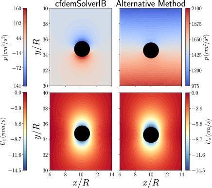
Figure 1: Comparison of $p/\rho_{f}$ and $U_{z}$ fields for our approach and cfdemSolverIB hager_2014 . a) and b) represent the pressure field, c) and d) the velocity field $U_{z}$.

Next, we investigate the stability of our method when computing very low Reynolds number conditions. Thus, we perform a systematic study, running a set of distinct scenarios increasing the fluid viscosity $\nu$. Fig. 2a and Fig. 2b illustrate the outcomes obtained using both approaches, in comparison with the analytical prediction of Stokes’ law. Our results indicate that both methods yield a reasonable description of the settling process and the particle reaches a viscous-dependent terminal velocity $v_{S}^{{}^{\prime}}$ at the long-time limit. As expected, the results obtained using both methods collapse in a single curve using $v_{S}=\frac{2}{9\mu}(\rho_{p}-\rho_{f})gR^{2}$ and $\tau=\frac{2}{9\mu}\rho_{p}R^{2}$. It is noticeable that both approaches slightly fails to reproduce the analytical solution during the initial acceleration process (see the insets in Figs.  2c and  2d).

However, assuming a negligible impact of the finite size boundary conditions implemented (in line with the results introduced in ganatos_1980 ), the present approach compares better with the asymptotic limit behavior. We speculate that the difference arises from the impact of dynamic pressure gradients acting on the particle surface for the original particle discretization. Hence, when a volumetric correction is applied to compute the pressure gradients to calculate the force $\mathbf{F}_{i,f}$, we account for the local solid fraction, resolving the corresponding pressure gradient more accurately.

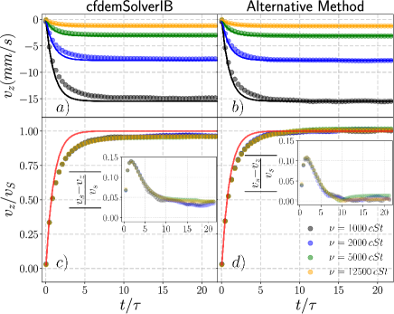
Figure 2: a) and b) Time evolution of the settling velocity of the sphere for both methods. c) and d) Time evolution of the settling velocity scaled by the corresponding Stokesian terminal velocity. The insets represent the relative differences in each case. Note that a more accurate asymptotic limit velocity is reached in our method. All solid lines represent the expected Stokesian dynamics.

3.2 Neighboring walls effect

Complementarily, we examine the impact of the confinement on the dynamics of a settling particle. Specifically, we explore the behavior of a particle located between two parallel walls. The particle is centered in the xy-plane of a box with dimensions $10d\times Hd\times 25d$ and is left to settle from rest. We systematically vary the distance between the walls $H/d=[1.2,1.4,1.8,2.6]$, in terms of particle diameter.

Fig 3a shows the terminal velocity of the sphere moving between two walls and obtained for different confinement conditions, fixing the fluid viscosity $\nu=1000\,cSt$. For simplicity sake, the data values are rescaled using the terminal velocity $v_{S}^{{}^{\prime}}$ that corresponds to the infinite system size limit. We observe that the simulations can reproduce a decrease in the terminal velocity when reducing the distance between the confining walls. Although, the sphere settles with a velocity larger than the analytical solutions provided by Faxén faxen_1923 and Ganatos et al. ganatos_1980 . Meanwhile, Fig 3b shows that our implementation has a consistent behavior for the range of viscosities investigated here. A similar result was previously obtained for a sphere in a creeping flow condition using an incompressible method based on OpenFOAM software ponianev_2016 .

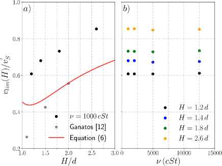
Figure 3: a) Settling velocity of a sphere between two planes scaled by the terminal velocity in a large system when varying the distance between walls $H$ for a liquid with $\nu=1000\,cSt$. The solid red line represents the inverse of the denominator of Equation 6. b) When analyzing the same velocities ratios of a) varying the viscosity, we observe a similar pattern for the confinement effect on the terminal velocity.

4 Conclusions

We introduce an alternative methodology to solve the particle-fluid interaction in the resolved CFDEM®coupling framework. The new approach explicitly accounts for the body force acting on the fluid phase, when computing the local momentum balance equations. The proper representation of the pressure profile in the fluid phase led to a single force model that no longer requires an explicit buoyant force to account for the gravitational interaction. Our method was able to outperform the cfdemSolverIB method for the settling velocity of a sphere, exhibiting more accurate results.

Complementarily, we study the dependence of the settling velocity of a sphere under confined conditions. The results indicated a consistent velocity decrease when reducing the distance between confining walls. Nevertheless, our numerical outcomes did not reproduce the analytical solutions found in the literature.

This work has been partially supported by Fundación Universidad de Navarra and the project from FIS 2017-84631 (MINECO). I. Fonceca also thanks Asociación de Amigos de la Universidad de Navarra for his scholarship.

References

- (1) C. Goniva, C. Kloss, N. Deen, J. Kuipers, S. Pirker, Particuology 10, 582-591 (2012)
- (2) A. Hager, C Kloss, S. Pirker, C. Goniva, Parallel open source CFD-DEM for resolved particle-fluid interaction (Ninth International Conference on CFD in the Minerals and Process Industries, Australia, 2012)
- (3) Z.G. Feng, E. Michaelides, J. Comput. Phys. 195, 602-628 (2003)
- (4) M. Ellero, T. Burghelea, V. Bertola, Transport Phenomena in Complex Fluids 361-392 (Springer International Publishing, 2020)
- (5) J. Koivisto, M. Korhonen, M. Alava, C. Ortiz, D. Durian, A. Puisto, Soft Matter 13, 7657-7664 (2017)
- (6) T. Zhao, G Houlsby, S. Utili, Granul. Matter 16, 921-932 (2014)
- (7) A. Hager, C. Kloss, S. Pirker, C. Goniva, The Journal of Computational Multiphase Flows 6, 13-27 (2014)
- (8) C. Kloss, C. Goniva, A. Hager, S. Amberger, Prog. Comput. Fluid Dy. 12, 140-152 (2012)
- (9) P. Cundall, O. Strack, Geotechnique 29, 47-65 (1979)
- (10) A. Shirgaonkar, M. Maciver, M. Patankar, J. Comput. Phys. 228, 2366-2390 (2009)
- (11) H. Faxén, Ark Mat 17, 1-28 (1923)
- (12) P. Ganatos, R. Pfeffer, S. Weinbaum, J. Fluid Mech. 99, 755-783 (1980)
- (13) S. Ponianev, K. Soboleva, A. Sobolev, V. Dudelev, G. Sokolovskii, Drag Coefficient of solid micro-sphere between parallel plates, (18th International Conference PhysicA, 2016)