Numerical Inside View of Hypermassive Remnant Models for GW170817

Abstract

The first multimessenger observation attributed to a merging neutron star binary provided an enormous amount of observational data. Unlocking the full potential of this data requires a better understanding of the merger process and the early post-merger phase, which are crucial for the later evolution that eventually leads to observable counterparts. In this work, we perform standard hydrodynamical numerical simulations of a system compatible with GW170817. We focus on a single equation of state (EOS) and two mass ratios, while neglecting magnetic fields and neutrino radiation. We then apply newly developed postprocessing and visualization techniques to the results obtained for this basic setting. The focus lies on understanding the three-dimensional structure of the remnant, most notably the fluid flow pattern, and its evolution until collapse. We investigate the evolution of mass and angular momentum distribution up to collapse, as well as the differential rotation along and perpendicular to the equatorial plane. For the cases that we studied, the remnant cannot be adequately modeled as a differentially rotating axisymetric NS. Further, the dominant aspect leading to collapse is the GW radiation and not internal redistribution of angular momentum. We relate features of the gravitational wave signal to the evolution of the merger remnant, and make the waveforms publicly available. Finally, we find that the three-dimensional vorticity field inside the disk is dominated by medium-scale perturbances and not the orbital velocity, with potential consequences for magnetic field amplification effects.

I Introduction

This work is motivated by the first multi-messenger detection compatible with the coalescence of two neutron stars (NSs). The gravitational wave (GW) event GW170817 detected by the LIGO/Virgo observatories matches the inspiral of two compact objects in the NS mass range Abbott et al. (2017a, 2019a). After a delay around $1.7\usk\mathrm{s}$, the GW signal was followed by short gamma ray burst (SGRB) event GRB170817A observed by Fermi and INTEGRAL satellites and attributed to the same source Abbott et al. (2017b). Later observations also revealed radio signals Mooley et al. (2018); Ghirlanda et al. (2019) that likely correspond to the radio-afterglow of the SGRB. The coincident GW and SGRB events triggered a large observational followup campaign Abbott et al. (2017c). Observations ranging from infrared to ultraviolet revealed an optical counterpart AT2017gfo with luminosity and spectral evolution compatible with a kilonova Abbott et al. (2017c); Kasen et al. (2017); Villar et al. (2017); Cowperthwaite et al. (2017).

The comparison of those observations to theoretical expectations requires the modeling of many different aspects of fundamental physics, such as general relativity, hydrodynamics, nuclear physics, neutrino physics, and magnetohydrodynamics. Modeling all potentially observable electromagnetic counterparts also involves a large range of timescales ranging from milliseconds to years. There is however little doubt that the early evolution phase up to tens of milliseconds after merger is of crucial importance. This phase can be studied via brute force three-dimensional numerical simulations and will be the topic of this work.

For predicting the expected kilonova signal, the important input from such studies are amount, composition, and velocity of matter dynamically ejected to infinity and of matter ejected from the disk. The latter is likely relevant since the kilonova spectral evolution is best fitted by two or more distinct ejecta components Kasen et al. (2017); Villar et al. (2017); Cowperthwaite et al. (2017) with masses that would be at tension with purely dynamical ejection mechanism. Although the fraction of disk mass expelled via winds is uncertain, the total mass of the disk poses an upper limit. Numerical simulations suggest that the initial disk mass depends strongly on the total mass of the system in comparison to the maximum NS mass for the given EOS, and on the mass ratio.

On timescales of 0.1 s, the evolution of the disk is strongly influenced by the interaction with the remnant. In case of a supra- or hypermassive NS, matter can be transported into the disk by different mechanisms. One is a purely hydrodynamic consequence of a complicated internal fluid flow inside the remnant Kastaun and Galeazzi (2015); Kastaun et al. (2016). Another potential mechanism is the amplification of magnetic fields inside the remnant and disk and the resulting pressure Ciolfi et al. (2019). Until collapse, a remnant NS also irradiates disk and ejecta with neutrinos and therefore has an impact on the composition. In particular the fraction of Lanthanides in the ejecta has a strong impact on the optical opacity. For those reasons, the remnant lifetime is important with regard to the kilonova signal.

Also with regard to the SGRB signal, the mass of the disk and the delay before black-hole (BH) formation are likely to be very relevant parameters. Current models for the SGRB engine require either a BH Shibata et al. (2006) or a magnetar Metzger et al. (2008) embedded in a massive disk. The question which scenario is viable, or if both are viable, is an active field of research. Should it be the case that BH formation is required before the SGRB, one obtains an upper limit on the collapse delay after merger. Given the total mass of the coalescing NSs as inferred from the GW signal, one obtains an upper limit on the mass which the central NS can be sustain longer than the SGRB delay. By comparing with the maximum mass of a nonrotating NS, a robust but not very strict constraint on the EOS was obtained from GW170817 Abbott et al. (2017b). Adding further assumptions, e.g., that the remnant NS is hypermassive, results in stricter limits Margalit and Metzger (2017); Shibata et al. (2019); Ruiz et al. (2018); Abbott et al. (2020). It is therefore very important to understand the stability criteria of the remnant.

For the simpler case of isolated uniformly rotating NS, the stability conditions are well understood. There is a maximum mass that depends only on the EOS. In the supramassive range, i.e. between the maximum masses of nonrotating and uniformly rotating NS, a minimum angular momentum is required. On timescales ${\lesssim}0.1\mathrm{s}$ however, one has to take into account that the remnant is not uniformly rotating and that a significant fraction of total mass and angular momentum can be located in the disk outside the NS remnant.

For the important case of hypermassive NS remnants, differential rotation is needed to prevent collapse. It is a popular assumption that collapse is caused by the dissipation of the differential rotation. Should this be the only important aspect, then the collapse delay depends on the effective viscosity, which is not well constrained as it may depend on small scale magnetic field amplification. However, numerical simulations prove that merger remnants emit strong GWs. Since short-lived remnants are close to collapse already, collapse could be triggered by a relatively small angular momentum loss. It might well be the case that the collapse delay is mainly determined by such losses instead of viscosity, or that both aspects are relevant.

The overall rotation profile of merger remnants, which is a key aspect for stability, has been studied in many numerical simulations Ciolfi et al. (2017); Kastaun and Galeazzi (2015); Kastaun et al. (2016, 2017); Ciolfi et al. (2019); Endrizzi et al. (2018, 2016); Hanauske et al. (2017). All these studies find a relatively slow rotation of the core, and a maximum rotation rate in the outer parts of the remnant. The typical mass distribution in the remnant core seems in fact to be similar to that of a nonrotating NS Kastaun and Galeazzi (2015); Kastaun et al. (2016); Ciolfi et al. (2017); Endrizzi et al. (2018). This led to the conjecture that the collapse occurs once the remnant core density profile matches the one in the core of the maximum-mass nonrotating NS Ciolfi et al. (2017). This conjecture was validated for a small number of examples Ciolfi et al. (2017); Endrizzi et al. (2018) but remains unproven in general.

The works above also revealed that the fluid flow can be more complex than just axisymmetric differential rotation, featuring secondary vortices (see Kastaun et al. (2016, 2017); Ciolfi et al. (2017)). However, those results are restricted to the equatorial plane, and little is know about the 3D structure. The analysis of fluid flow patterns in numerical simulations is complicated because early merger phase is not fully stationary. Remnants show strong oscillations and can undergo a drift of compactness and rotation rate within few dynamical timescales. A further difficulty arises from the coordinate choices in numerical simulations, which are not well suited for studying the remnant shape Kastaun and Galeazzi (2015).

In this work, we focus on studying the three-dimensional structure of merger remnants obtained when including only the most basic ingredient of general relativistic hydrodynamics, while neglecting magnetic fields, effective magnetic viscosity, and neutrino radiation transport. We will analyze the outcome of two simulations compatible with GW170817 in depth. For this, we develop novel postprocessing and visualization methods. We also investigate the evolution of the angular momentum distribution, using different measures.

For GW170817, all useful information about the postmerger phase comes from the optical counterparts. No GW signal could be detected after merger Abbott et al. (2017d, 2019b). Future observations of similar events with third-generation GW antennas might also include direct detection of a postmerger GW signal or strict upper limits. In order to support the development of postmerger-GW data analysis methods, we make the waveforms extracted from our simulations publicly available Kastaun and Ohme (2021) as a qualitative example.

II Methods

II.1 Evolution

The general relativistic hydrodynamic equations are evolved numerically using the code described in Galeazzi et al. (2013); Alic et al. (2013). The code utilizes a finite-volume high resolution shock capturing scheme in conjunction with the HLLE approximate Riemann solver and the piecewise parabolic method for reconstructing values at the cell interfaces. We neither include magnetic fields nor neutrino radiation, and the electron fraction is passively advected along with the fluid. Our numerical evolution employs a standard artificial atmosphere scheme, with zero velocity, lowest available temperature, and a spatially constant density cut of $6\times 10^{5}\usk\mathrm{g}\mathrm{/}\mathrm{c}\mathrm{m}\mathrm{{}^{3}}$.

The matter equation of state is computed using a three-dimensional interpolation table, where the independent variables are density, temperature, and electron fraction. For the simulations in this work, we employ the SFHO EOS Hempel and Schaffner-Bielich (2010), which incorporates thermal and composition effects. The EOS was taken from the CompOSE EOS collection Typel et al. (2018). The table only contains temperatures above $0.1\usk\mathrm{M}\mathrm{eV}$. In the context of a binary NS (BNS) merger simulation, this is not problematic since the thermal pressure at this temperature is negligible to the degeneracy pressure except for very low densities. Although dynamically ejected matter becomes diluted, it is also very hot and therefore not affected.

The spacetime is evolved using the McLachlan code Brown et al. (2009), which is part of the Einstein Toolkit Löffler et al. (2012). This code implements two formulations of the evolution equation: the BSSN formulation Nakamura et al. (1987); Shibata and Nakamura (1995); Baumgarte and Shapiro (1998), and the newer conformal and spatially covariant Z4 evolution scheme described in Alic et al. (2012, 2013). Here we use the latter because of its constraint damping capabilities. We employ standard gauge conditions, choosing the lapse according to the $1+\log$-slicing condition Bona et al. (1995) and the shift vector according to the hyperbolic $\Gamma$-driver condition Alcubierre et al. (2003). At the outer boundary, we use the Sommerfeld radiation boundary condition.

The time integration of the coupled hydrodynamic and spacetime evolution equations is carried out using the Method of Lines (MoL) with a 4th-order Runge-Kutta scheme. Further, we use Berger-Oliger moving-box mesh refinement provided by the Carpet code Schnetter et al. (2004). For tests of the code, we refer the reader to Galeazzi et al. (2013); Alic et al. (2013).

In total, we use six refinement levels, each of which has twice the resolution of the next finer one. The four coarsest levels consist of a simple hierarchy of nested cubes centered around the origin. The two finest levels consist of nested cubes that follow each of the stars during inspiral. Near merger, those are replaced by non-moving nested cubes centered around the origin. The finest grid spacing is $221\usk\mathrm{m}$. The outer boundary is located at $950\usk\mathrm{k}\mathrm{m}$, and the finest level after merger covers a radius of $28\usk\mathrm{k}\mathrm{m}$. Finally, we use reflection symmetry across the orbital plane.

II.2 Initial data

In this work, we evolve binaries with a chirp mass of $M_{c}=1.187\usk M_{\odot}$, which is compatible with the very precise measurement result of $M_{c}=1.186^{+0.001}_{-0.001}\usk M_{\odot}$ for GW event GW170817 Abbott et al. (2019a). We consider the equal-mass case and one unequal-mass system with mass ratio $q=0.9$. The NSs in our models are non-spinning, i.e. we use irrotational initial data. However, note that spin can have an impact on many aspects discussed here, as demonstrated, e.g., in Kastaun et al. (2017); Chaurasia et al. (2020); Dietrich et al. (2017); East et al. (2016) for different systems. The characteristic properties of our models are listed in Table 1.

As initial data EOS, we use the lowest temperature of $0.1\usk\mathrm{M}\mathrm{eV}$ that is available in the SFHO EOS. The initial electron fraction for a given density is set according to $\beta$-equilibrium. This approximation to the zero-temperature EOS breaks down at very low densities because the thermal pressure contribution becomes important and stays constant once it is dominated by the photon gas. To avoid technical problems determining the NS surface, we therefore replace the finite temperature table at densities below $1.4\times 10^{7}\usk\mathrm{g}\mathrm{/}\mathrm{c}\mathrm{m}\mathrm{{}^{3}}$ by a matching polytropic EOS (with adiabatic exponent $1.58$).

The effective tidal deformability $\tilde{\Lambda}$, which encodes the impact of tidal effects on the gravitational waveform during coalescence, is almost identical for the two mass ratios (in contrast to the individual deformabilities). The value of $\tilde{\Lambda}$ is compatible with upper limits inferred for GW170817 under the assumption of small NS spins Abbott et al. (2017a, 2019a, 2018); De et al. (2018). The statistical interpretation of the lower confidence bounds given in Abbott et al. (2019a, 2018); De et al. (2018) is called into question Kastaun and Ohme (2019), but in any case $\tilde{\Lambda}$ is well above those limits for our models. We also note that the Bayesian model selection study Abbott et al. (2020) does not rule out even the zero tidal deformability case.

We note that our model is not compatible with the lower limit $\tilde{\Lambda}>450$ derived in Radice et al. (2018) using inferred ejecta mass requirements for kilonova observation AT2017gfo. However, this value is based on an invalid assumption about the relation between disk mass and effective tidal deformability. A first counterexample was found in Endrizzi et al. (2018) and a systematic investigation Kiuchi et al. (2019) provided more. Revised fitting formulas presented in Nedora et al. (2020) exhibit large residuals and the search for robust analytic modeling of ejecta masses is an ongoing effort. In any case, the disk and ejecta mass is computed in our simulations and will be compared to values inferred from the kilonova directly.

In order to compute BNS systems in quasi-circular orbit, we employ the LORENE code Gourgoulhon et al. (2001). Since we are mainly interested in the qualitative post-merger behavior, we take no steps to reduce the residual eccentricity inherent in the quasi-stationary approximation, and we chose an initial separation that corresponds to no more than 6 full orbital cycles before merger.

Table 1: Initial data parameters: $M_{\mathrm{B}}$ denotes the total baryonic mass of the binary, $M_{c}$ the chirp mass, $M_{1}$ and $M_{2}$ the gravitational masses of the stars, $q=M_{2}/M_{1}$ the mass ratio, $\Lambda_{1}$ and $\Lambda_{2}$ the dimensionless tidal deformability of the stars, and $\tilde{\Lambda}$ the effective tidal deformability.

Model	Q10	Q09
$M_{\mathrm{B}}\,[M_{\odot}]$	$3.001$	$3.008$
$M_{c}\,[M_{\odot}]$	$1.187$	$1.187$
$M_{1}\,[M_{\odot}]$	$1.364$	$1.438$
$M_{2}\,[M_{\odot}]$	$1.364$	$1.294$
$q$	$1.0$	$0.9$
$\Lambda_{1}$	$396$	$280$
$\Lambda_{2}$	$396$	$551$
$\tilde{\Lambda}$	$396$	$396$

Using the same EOS as for the initial data, we computed the baryonic mass for sequences of NSs rotating uniformly with rate at the mass shedding limit (using the RNS code Stergioulas and Friedman (1995)). We find that the maximum baryonic mass for a uniformly rotating NS is $2.86\usk M_{\odot}$. Based on comparisons in Kaplan et al. (2014); Kastaun et al. (2016), we do not expect thermal contributions in the heated merger remnant to significantly increase this maximum. The total baryonic mass of our BNS models is well above the maximum allowed for uniformly rotating models. Even allowing for atypically large mass ejection of $0.1\usk M_{\odot}$, the remnant is therefore hypermassive, i.e., it requires non-uniform rotation to delay collapse. We therefore expect BH formation within tens of ms after merger.

II.3 Coordinate Systems

The standard 1+log and gamma-driver gauge conditions used during evolution are well suited to prevent catastrophic gauge pathologies, but they are not designed to recover axisymmetric coordinates when the spacetime approaches a mostly axisymmetric stationary phase. The coordinate system present after merger depends not on the final mass distribution, but on the whole history of the evolution. Therefore, one cannot rely on the coordinate-dependent quantities, e.g. multipole moments expressed in coordinates, to measure any deviations from axisymmetry.

In Kastaun and Galeazzi (2015), we developed a postprocessing procedure to obtain a well defined coordinate system in the equatorial plane with the following properties 1. The radial coordinate is the proper distance to the origin along radial coordinate lines 2. The angular coordinate is based on proper distance along arcs of constant radial coordinate 3. On average, the radial coordinate lines are orthogonal on the angular ones, thus minimizing twisting. If the spacetime is indeed axisymmetric (with axis orthogonal to the equatorial plane of the simulation coordinates) then so are the new coordinates.

In this work, we also want to study the 3D structure of the remnant. We therefore need to extend the coordinate system above from the equatorial plane. However, the metric was not saved in 3D in our simulations, which precludes a generalization in the same spirit. Instead, we use an ad-hoc construction as follows. First, we apply the same coordinate transformation as within the equatorial plane to all planes with constant $z$-coordinate. Using the metric saved along the $z$-axis during the simulation, we transform the $z$-coordinate as $z\to z^{\prime}(z)$ such that on the $z$-axis, the new $z$-coordinate is the proper distance to the equatorial plane along the axis. Away from the axis, the new $z$-coordinate is only an approximation to the proper distance to the equatorial plane.

The resulting 3D coordinate system allows to judge axisymmetry in the equatorial plane, and it allows to assess oblateness since distances along the $z$-axis and within the equatorial plane are exact proper distances. In the meridional planes a coordinate circle might still show some deviations from a proper sphere, except on $z$-axis and the equator. In the rest of this work, we refer to this coordinate system as postprocessing coordinates to distinguish from simulation coordinates.

From previous experience Kastaun et al. (2016, 2017); Ciolfi et al. (2017), we expect that the remnant is changing only slowly when viewed in a coordinate system rotating with a certain angular velocity, which is also changing slowly (also compare the animations provided in the supplemental material of Kastaun et al. (2017)). In other words, we expect an approximate helical Killing vector.

To extract the rotating pattern of mass distribution and velocity field, we construct corotating coordinates as follows. First, we perform a Fourier decomposition with respect to $\phi$ (in postprocessing coordinates) in the equatorial plane. We then compute a density-weighted average to get the phase of the dominant $m=2$ density deformation as function of time. We further apply a smoothing by convolution with a $2\usk\mathrm{m}\mathrm{s}$ long Hanning window function to suppress high frequency contributions. We then apply the opposite rotation to the 3D postprocessing coordinates at each time to obtain postprocessing coordinates corotating with the main deformation pattern.

II.4 Diagnostic Measures

In order to extract gravitational waves, we decompose the Weyl-scalar $\Psi_{4}$ into spin-weighted spherical harmonics, considering all multipole coefficients up to $l=4$. The strain is computed by time integrating using the fixed-frequency integration Reisswig and Pollney (2011) method with a low-frequency cutoff at $500\usk\mathrm{Hz}$. The fluxes of energy and angular momentum are also computed using multipole components up to $l=4$. We use a fixed extraction radius $R_{\mathrm{ex}}=916\usk\mathrm{k}\mathrm{m}$, close to the outer boundary of the computational domain. We do not extrapolate the signal to infinity as we expect the finite resolution error to dominate the error due to finite extraction radius.

To describe the distribution of matter, we use the baryonic mass density $\rho$, defined as baryon number density in the fluid rest frame times an arbitrary mass constant (in this work $1.66\times 10^{-27}\usk\mathrm{k}\mathrm{g}$). Baryon number conservation implies a conserved current $u^{\mu}\rho$, with $u$ being the fluid 4-velocity. The total baryonic mass within a volume can only change by matter leaving the boundary, and is given by

$$M_{\mathrm{B}} =\int_{V}W\rho\,\mathrm{d}V, \mathrm{d}V =\sqrt{\gamma}\,\mathrm{d}^{3}x$$ (1)

where $W$ is the Lorentz factor of the fluid with respect to Eulerian observers, $\mathrm{d}V$ is the proper 3-volume element and $\gamma$ is the determinant of the 3-metric. On the numerical level, the baryonic mass definition is complicated by the use of an artificial atmosphere. Our numerical volume integrals of baryonic mass exclude any grid cell set to atmosphere.

To obtain the mass of dynamically ejected matter, we compute the time-integrated flux of unbound matter through several coordinate spheres with radii between $73$–$916\usk\mathrm{k}\mathrm{m}$. For each sphere, we then add the volume integral of residual unbound matter still present within the same sphere at the end of the simulation. Matter is considered unbound according to the geodesic criterion $u_{t}<-1$, where $u$ is the 4-velocity, and the artificial atmosphere is excluded. This criterion assumes force-free ejecta and therefore becomes more accurate at larger radii.

The combined measure for the ejecta mass alleviates drawbacks of using flux or volume integrals only. When using only the flux through an extraction sphere, one is either restricted to small extraction radii to ensure that all ejecta are accounted for, or forced to evolve the system long enough to allow all ejecta to reach the extraction radius. When using only volume integrals, they have to be computed before significant amounts of ejecta leave the computational domain. Such integrals then include matter at small radii where the geodesic criterion is unreliable, and miss ejecta that become unbound later. The combined measure allows meaningful comparison over a larger range of extraction radii. For the cases at hand, we find negligible differences for radii $\gtrsim 400\usk\mathrm{k}\mathrm{m}$, and use the outermost radius $916\usk\mathrm{k}\mathrm{m}$ for quoting ejecta masses.

We employ a similar approach for estimating the escape velocity. In a stationary spacetime, the velocity that a fluid element would reach after escaping the system on a geodesic trajectory is $v^{2}_{\infty}=1-u_{t}^{-2}$. Again, we consider both the ejecta leaving the system through a spherical extraction surface during the simulation, and the unbound matter still within the domain at the end. Both contributions are filled into a mass-weighted histogram of the escape velocity. This way, we account for the fastest components via the flux as well as the slowest ones via the unbound matter at final time.

For technical reasons, we first combine all ejecta at a given time within thin spherical shells $V_{s}$ with radius $R_{s}$ and thickness $\delta R_{s}$. For those, we compute the volume integrals

$$W_{s} =\frac{1}{M_{s}}\int_{V_{s}}u_{t}W\rho_{u}\,\mathrm{d}V, M_{s} =\int_{V_{s}}W\rho_{u}\,\mathrm{d}V$$ (2)

where $\rho_{u}$ is the density of unbound matter in the fluid rest frame. From the above measures, we attribute an average escape velocity $v^{2}_{s}=1-W_{s}^{-2}$ to each shell. To compute the above integrals at each time for each radius, we employ a simple and robust technical implementation based on creating histograms of all numerical grid cells, binned by radius, and weighted by the integrands.

Another quantity relevant for our study is the ADM mass of the system. This measure is formally defined for the whole spacetime, as there is no locally conserved energy in GR. It can be expressed either via surface integrals at infinity, or 3-volume integrals over a spacelike hypersurface of a given foliation of spacetime. When restricting either formulation to sufficiently large but finite region, such that the outer boundary lies in the weak field regime, then the ADM mass is not constant but changes by the amount of energy carried away by GW. We thus compute a time-dependent ADM mass from the ADM mass of the initial data minus the integrated GW energy flux.

As a heuristic measure of energy distribution, we monitor the integrand of the ADM mass volume integral as well. However, we stress that this is not gauge invariant as it depends on the chosen foliation of spacetime. Our motivation is to split the total ADM energy into contributions of the remnant NS and the surrounding disk.

We also need to consider the gravitational radiation still inside the computational domain. As a practical measure, we use the following: considering the region between $R_{0}<r<R_{\mathrm{ex}}$, we define a GW energy at time $t$ as the integrated GW flux through $R_{\mathrm{ex}}$ over the time interval $(t,t+R_{\mathrm{ex}}-R_{0})$. We compute this measure for $R_{0}$ as low as $100\usk\mathrm{k}\mathrm{m}$ (around the wavelength of a $3\usk\mathrm{k}\mathrm{Hz}$ signal). In other words, we associate an energy loss of the remnant at a given time with the GW luminosity at a large extraction radius at the time when the radiation from radius $R_{0}$ has reached the extraction radius. This can only provide a qualitative picture, as the measure is build on concepts valid in the weak field limit / wave zone.

For the angular momentum, we use the volume integral formulation of the ADM angular momentum, similarly to the ADM mass above. As for the mass, we compute the GW angular momentum loss, at the same extraction radius. For axisymmetric spacetimes, another angular momentum definition is given by Komar. Since the system approaches a roughly axisymmetric state after merger, it makes sense to use the Komar angular momentum. We note that the Komar measure is more closely related to the fluid in the sense that there are no contributions of vacuum, horizons aside, and, consequently, no contributions of GW radiation present in the system. For exact definitions of ADM and Komar quantities, we refer to Gourgoulhon (2012).

The post-merger evolution is not exactly axisymmetric, the postprocessing coordinates are not available during the simulation, and we avoid storing all metric quantities as 3D data. Therefore, we use an approximation to the Komar angular momentum that is obtained by integrating the $\phi$-component (in simulation coordinates) of $S_{\phi}$, the evolved quasi-conserved momentum density. This is trivial to compute during the simulation, but becomes exact only if the $\phi$-coordinate is a Killing vector field.

Besides volume integrals over the full domain, we are interested in the radial distribution of the integrands. For this, we employ a numerical method developed in a previous study Kastaun et al. (2016). This method allows an efficient computation of volume integrals (i) within spheres of constant coordinate radii as function of radius, and (ii) within regions above given mass densities $\rho$ as function of $\rho$. It works by adding the integrand (including the volume element) in each numerical cell into onedimensional histograms binned in terms of coordinate radius and density, respectively. The volume integrals can then be obtained during post-processing simply by cumulative summation over the bins. Using this method, we integrate the (i) proper volume (ii) baryonic mass (iii) ADM mass (iv) ADM angular momentum (v) Komar angular momentum approximation (vi) estimated mass of unbound matter .

We note that the 3-dimensional isodensity surfaces in 4-dimensional spacetime are gauge-independent. The corresponding volume integrals within a time slice depend only on the time slicing but not on the spatial gauge. In contrast, integrals over spheres of constant coordinate radius depend on the spatial coordinates. In order to reduce this dependency, we parametrize the spheres by the enclosed proper volume. The only remaining gauge ambiguity (beside the time slicing) is given by the shapes of the coordinate spheres, but not their overall extent.

Similarly, we also parametrize the integrals within isodensity surfaces by the enclosed proper volume. Within the remnant NS, where the mass distribution is roughly spherical, the two methods of defining radial mass distribution should roughly agree. This is not the case for the torus-shaped disk. For convenience, we will sometimes express proper volumes in terms of the radius of Euclidean spheres with same volume (“volumetric radius”, $R_{V}$).

Based on the above integrals, we can define a measure for the compactness of any volume as the baryonic mass divided by the volumetric radius. The compactness of isodensity surfaces as function of volumetric radius a has a maximum. We refer to the region within this maximum-compactness surface as the “bulk”. We use the bulk definition to divide the matter distribution after merger into a remnant and a disk, but we stress that this is somewhat arbitrary as there is a smooth transition.

III Results

III.1 Overall dynamics

In the following, we provide a broad overview on the merger outcome. Key quantities are summarized in Table 2. Qualitatively, both cases are very similar. For the example of the $q=0.9$ case, we visualize the evolution timeline in Fig. 1. The coalescing NS merge into a hypermassive NS (HMNS) which collapses to a BH after a delay on the order of ${\approx}10\usk\mathrm{m}\mathrm{s}$. The HMNS is embedded in a massive debris disk created during merger. The disk is strongly perturbed by interactions with the remnant, and settles to a more stationary state shortly after the BH is formed.

Quantitatively, we observe some differences between the two mass ratios. Most notably, the collapse delay is about 0.25% shorter for the unequal mass case. This can be seen in Fig. 2 showing the evolution of the remnant density. We stress that in general, the delay time for a given mass is very sensitive to numerical errors, because the system is at the verge of collapse (we will discuss the evolution leading to collapse in later sections). However, since both simulations employ the same resolution, grid setup, and numerial method, we expect the difference of the delays to be more robust than the absolute values.

For a remnant close to collapse, one can expect that small changes of the initial parameters, mainly the total mass, should lead to large changes of the delay. This is however not a drawback. Any observational constraint on the delay translates into a stronger constraint on the total mass. In this context, the relevant numerical uncertainty is not the (large) error of the delay for a given mass, but the (smaller) error in the total mass that leads to a given collapse delay.

We emphasize that our non-magnetized simulations exclude the possibility of effective magnetic viscosity due to small-scale magnetic field amplification. Such effects might reduce the collapse delay further. Since it is difficult to predict the impact of mass ratio on magnetic field amplification, we also cannot exclude an impact on the relation between collapse delays and mass ratio. For further discussion, see Kiuchi et al. (2018) and the references therein.

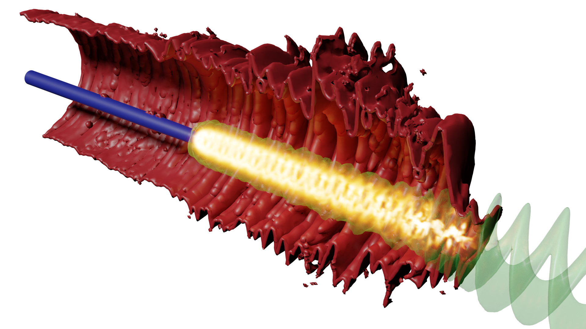
Figure 1: Overview of the evolution phases for the $q=0.9$ case. Time runs from lower right to upper left, while the other two dimensions correspond to the orbital plane. The transparent green surface corresponds to a fixed density of $5\times 10^{13}\usk\mathrm{g}\mathrm{/}\mathrm{c}\mathrm{m}\mathrm{{}^{3}}$, highlighting the evolution of the merged NS and the coalescing NS shortly before merger. The solid red surface corresponds to a density of $10^{11}\usk\mathrm{g}\mathrm{/}\mathrm{c}\mathrm{m}\mathrm{{}^{3}}$, as a proxy for the denser parts of the disk. To avoid occlusion, one half-plane was cut away. The blue surface marks the apparent horizon extracted during the simulation. To give an impression of the thermal evolution inside the remnant, we rendered hot, dense regions as light emitters (without absorption). The time coordinate was compressed by a factor $0.05$ with respect to the spatial coordinates in geometric units, such that light cones would appear almost orthogonal to the world tube of the remnant.

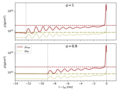
Figure 2: Post-merger evolution of mass density in the remnant for the equal mass case (top panel) and unequal mass case (bottom panel). The solid curve shows the maximum baryonic mass density in the fluid frame. The dotted curve shows an average density given by bulk mass per bulk volume (see text). The time refers to coordinate time. For comparison, the horizontal lines show the central density (dashed) and average bulk density (dash-dotted) of the maximum-mass TOV solution. The vertical lines mark the time of merger and formation of an apparent horizon.

The HMNS is smoothly embedded within a debris disk. The structure of the disk is shown in Fig. 3 for the example of the $q=0.9$ case. The innermost part of the disk falls into the BH after the remnant collapses. After collapse, the remaining disk mass is around $0.05\usk M_{\odot}$ (see Table 2). The disk contains enough matter to supply a wind that could explain the red component of the kilonova AT2017gfo observed after GW170817, with an inferred mass ${\approx}0.04\usk M_{\odot}$ Kasen et al. (2017). It would, however, require an effective mechanism in order to expel around 80% of the disk. The structure of the disk after BH formation is shown in Fig. 4 for the $q=0.9$ example.

As a general trend, we expect that for fixed EOS and mass ratio, systems with lower total mass possess a more massive disk after merger (compare, for example, Radice et al. (2018)). We will further show that in our cases, some matter is migrating from the remnant into the disk. This was already observed for different models in previous studies Kastaun et al. (2016); Endrizzi et al. (2018). Since the remnant lifetime also increases with decreasing mass, the final disk mass should depend even more strongly on the total mass. Conversely, we expect a more massive disk for a system with the same total mass, but obeying a different EOS for which the maximum NS mass is slightly larger.

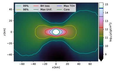
Figure 3: Mass distribution in the meridional plane $2\usk\mathrm{m}\mathrm{s}$ before apparent horizon formation, averaged over a time window $\pm 1\usk\mathrm{m}\mathrm{s}$. The color scale shows the baryonic mass density. The contours mark densities for which the corresponding isodensity surfaces contain selected mass fractions. We show the contours for $99\%$, $98\%$, the mass swallowed by the BH within $1\usk\mathrm{m}\mathrm{s}$ after formation, the maximum mass of uniformly rotating and nonrotating NS, and the (nearly identical) mass of the nonrotating NS best approximating the core (see text).

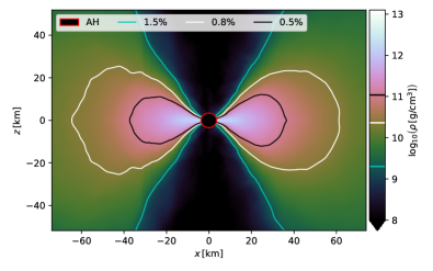
Figure 4: Like Fig. 3, but showing the time $2\usk\mathrm{m}\mathrm{s}$ after apparent horizon formation. The density contours contain selected fractions of initial total baryonic mass (excluding the BH interior).

Table 2: Key parameters of merger outcome. $M_{\mathrm{BH}}$ and $J_{\mathrm{BH}}$ are black hole mass and angular momentum $5.0\usk\mathrm{m}\mathrm{s}$ after formation. $F_{\mathrm{BH}}$ is the GW frequency from quasi-normal-mode ringdown for the given mass and spin. $M_{\mathrm{blk}}$ and $R_{\mathrm{blk}}$ are bulk mass and bulk volumetric radius, extracted $1.0\usk\mathrm{m}\mathrm{s}$ before collapse. Rows $\nu_{\mathrm{cnt}}$ and $\nu_{\mathrm{max}}$ denote the remnants central and maximum rotation rates computed $1.0\usk\mathrm{m}\mathrm{s}$ before collapse. $f_{\mathrm{merge}}$ is the gravitational wave instantaneous frequency at the time of merger, $f_{\mathrm{pm}}$ is the frequency of the maximum in the post-merger part of the gravitational wave power spectrum. Row $M_{\mathrm{disk}}$ provides the baryonic mass outside the apparent horizon, excluding unbound matter, at time $6.0\usk\mathrm{m}\mathrm{s}$ after collapse. $M_{\mathrm{ej}}$ is the estimate for the total mass of dynamically ejected matter, $v_{\infty}$ refers to the median, 5th and 95th percentiles of the mass-weighted escape-velocity distribution of ejected matter.

Model	Q10	Q09
$M_{\mathrm{BH}}\,[M_{\odot}]$	$2.55$	$2.57$
$J_{\mathrm{BH}}/M^{2}_{\mathrm{BH}}$	$0.66$	$0.67$
$F_{\mathrm{BH}}\,[\mathrm{kHz}]$	$6.56$	$6.52$
$M_{\mathrm{blk}}\,[M_{\odot}]$	$2.56$	$2.59$
$M_{\mathrm{blk}}/R_{\mathrm{blk}}$	$0.31$	$0.31$
$\nu_{\mathrm{cnt}}\,[\mathrm{kHz}]$	$0.96$	$0.87$
$\nu_{\mathrm{max}}\,[\mathrm{kHz}]$	$1.76$	$1.71$
$f_{\mathrm{merge}}\,[\mathrm{kHz}]$	$1.94$	$1.94$
$f_{\mathrm{pm}}\,[\mathrm{kHz}]$	$3.38$	$3.35$
$M_{\mathrm{disk}}\,[10^{-2}\,M_{\odot}]$	$5.5$	$4.6$
$M_{\mathrm{ej}}\,[10^{-2}\,M_{\odot}]$	$1.7$	$0.8$
$v_{\infty}\,[c]$	$0.16^{+0.08}_{-0.11}$	$0.14^{+0.09}_{-0.08}$

We observe significant dynamical mass ejection during merger and during the remnant lifetime. As shown in Fig. 5, several independent mass ejections are launched, mostly from radii ${\lesssim}100\usk\mathrm{k}\mathrm{m}$. The individual ejected components merge, because of their velocity dispersion, and leave the system as a single ejecta component. It seems that the pressure waves injected into the disk (see also Fig. 1) by the HMNS also result in matter ejection from the disk.

The ejecta mass as extracted from the numerical results is given in Table 2. We stress that in general, ejecta masses extracted from numerical simulations are affected comparably strong by the numerical errors. Convergence tests presented in Ciolfi et al. (2017) for simulations of a long-lived remnant using a very similar numerical setup found a finite resolution error of the dynamical ejecta mass around $20\%$. In our case, an additional — and likely dominant — source of uncertainty is the dependence of dynamical ejecta mass on the lifetime of the remnant. The latter can be extremely sensitive to errors if the remnant is on the verge of collapse. It is therefore difficult to estimate the error without expensive tests with much higher resolutions, but we suspect that the error could easily reach a factor two.

Comparing to other results in the literature, we find a disk mass that is an outlier to the phenomenological fit of disk mass in terms of effective tidal deformability that was proposed in Radice et al. (2018). Other counterexamples were already found in Endrizzi et al. (2018); Kiuchi et al. (2019). We also note that Nedora et al. (2021) performed a simulation that corresponds almost exactly to our $q=1$ setup, except that it includes neutrino radiation. They quote a lower ejecta mass $(2.8\pm 0.7)\times 10^{-3}\usk M_{\odot}$ as well as a lower disk mass $(1.9\pm 0.7)\times 10^{-2}\usk M_{\odot}$, but also find a remnant lifetime that is around $3$ times shorter than for our simulations.

Our results depicted in Fig. 5 show that mass is continuously ejected during the HMNS lifetime. The differences in lifetime could thus account for the tension regarding the ejecta masses. Similarly, it might account as least partially for the lower disk mass. The difference in lifetime could be due to finite resolution errors alone, but it is also possible that the inclusion of neutrino transport has an influence on HMNS close to collapse. In any case, the result that increasing the lifetime of a HMNS can lead to larger disk and ejecta masses suggests that fitting these quantities in terms of the binary parameters as in Radice et al. (2018); Nedora et al. (2020) is challenging for the parameter ranges resulting in short-lived HMNS. We propose to include the lifetime as an unknown in the fit, not just because of the sensitivity with regard to total mass and numerical errors, but also because the lifetime may be affected by physical effects such as magnetic viscosity that are essentially unknown.

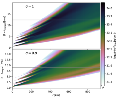
Figure 5: Radial distribution of unbound matter versus time after merger. The color scale corresponds to unbound mass per radial distance, where matter is considered unbound according to the geodesic criterion. The horizontal lines mark the time of BH formation.

The spectral evolution of the kilonova depends strongly on the ejecta velocity. Table 2 reports the median of the velocity distribution extracted from our simulations as described in Sec. II.4, together with 5th and 95th percentiles. The values refer to the outermost extraction radius, but we also compared smaller ones. We find that the median and 5th percentile are stable outside $400\usk\mathrm{k}\mathrm{m}$, whereas the 95th percentile continuously decreases and should be considered as unreliable. Given that the fastest components are those running into the artificial atmosphere, the deceleration is likely unphysical. Another source of uncertainty is that an earlier collapse of the HMNS would result in less ejected mass, but faster median velocity, because ejecta launched at later times tend to be slower for the cases at hand.

The mass and velocity found in our numerical results are both about a factor two lower than the estimates inferred by Kasen et al. (2017) for the blue component of the kilonova AT2017gfo. However, because of the uncertainties discussed above, we cannot make a conclusive statement if the dynamical ejecta mass for the SFHO EOS is compatible with the observed kilonova.

Besides mass and velocity, kilonova models such as Kasen et al. (2017) also predict a strong dependency on the composition of the ejecta. The initial electron fraction of the neutron-rich ejecta is strongly affected by neutrino radiation (see, e.g., Martin et al. (2018)). Since those are not included in our study, we refrain from discussing the ejecta composition, but note that once again the lifetime of the HMNS has a direct impact on an observable.

It should also be noted that disk evolution and ejecta might be sensitive to magnetic field effects, which are not included here. For the example of a system with large initial magnetic field that was studied in Ciolfi et al. (2019), the entire disk was driven to migrate outwards (but not necessarily ejected). On the other hand, a reduction of remnant lifetime by magnetic viscosity might result in less dynamical ejecta and a less massive disk.

III.2 Gravitational Waves

In this section, we present the GW signals extracted from the simulations as described in Sec. II.4. We compare the dominant spherical harmonic $\ell=|m|=2$ mode with predictions from theoretical waveform models, produce a hybrid waveform combining analytical inspiral data with the result from our numerical simulations, and quantify the initial eccentricity of our simulations through the GW frequency.

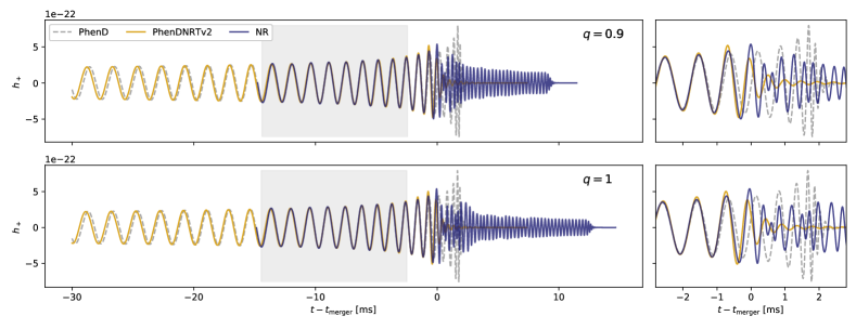
Figure 6: The GW signals extracted from our simulations (blue) as observed face-on at a distance of $40.7\,\textrm{Mpc}$. We extend the inspiral with the BNS model IMRPhenomD_NRTidalv2 Dietrich et al. (2019) (orange), aligned with the numerical data over the grey shaded region. For comparison, we also include the BBH model IMRPhenomD Husa et al. (2016); Khan et al. (2016) (gray dashed lines).

Figure 6 shows the plus polarization of the GW from three data sets. The purple line is the result extracted from the numerical simulation. Three characteristic phases are clearly identifiable. During the inspiral, the amplitude and frequency gradually increase until the maximal amplitude of the complex strain, $h=h_{+}-i\,h_{\times}$, is reached at $t=t_{\mathrm{merger}}$. The following post-merger oscillation is characterized by an overall slowly decaying amplitude. Figure 7 shows the instantaneous frequency, $F=(2\pi)^{-1}d\phi/dt$, where $\phi$ is the GW phase extracted as the argument of the complex strain $h$. It exhibits a characteristic modulation, with an initially large but rapidly damped amplitude. As we will show in Sec. III.3, this modulation is an imprint of the remnant’s radial oscillations. Such an imprint might be exploited in observations with next-generation instruments. Apart from the modulation, the frequency also shows a slow drift towards higher frequencies. This correlates with a change in remnant compactness that will be investigated in Sec. III.3. Once the BH is formed, the signal amplitude decays quickly while the frequency reaches the value that is expected for a BH with the mass and spin found in our simulations (this can only be observed briefly as the amplitude quickly becomes too small for numerical study).

The other two curves shown in Fig. 6 are predictions from waveform models commonly used in the LIGO and Virgo data analysis. In order to visually compare them to the numerical simulations and hybridize the waveforms, we aligned each model with the respective signal from our numerical simulation using the following procedure. First, after generating the model waveforms using the same masses as our numerical simulations and zero spins, we align the signals in time by minimizing the $\mathbb{L}_{2}$ norm of the difference between the phase velocities $\omega=2\pi F$, taken over the time interval where $\omega\in[3850,6000]\usk\rad\mathrm{/}\mathrm{s}$. Second, we adjust the phase offset in the model such that the average phase difference between the numerical data and the models vanishes in the interval specified above. The only free choice in this procedure is the interval used for the alignment. It has to be chosen small enough to align the waveforms in the “early” inspiral of the numerical simulation. On the other hand, the size of the interval has to be large enough so that the frequency evolves significantly MacDonald et al. (2011). Otherwise the time shift would only be weakly constrained. The range defined above is an empirically found compromise that is shown as a shaded band in Fig. 6.

One model used for comparison is the binary BH (BBH) model IMRPhenomD Husa et al. (2016); Khan et al. (2016) that does not incorporate tidal, finite-size effects of NSs. We would therefore not expect it to accurately describe the late inspiral and merger of a BNS. However, the tidal effects for the cases at hand are small in the frequency range used for the fitting, quite likely within the numerical error of the simulations. We stress that the aim of our study is not the accurate modeling of the inspiral phase, which would require very high resolution (see, e.g., Kiuchi et al. (2020)).

Just before merger, the BH model and NS simulation start to diverge significantly. A BBH with the same masses, following the alignment of the model and simulations used here, would perform about 1.5 orbits more than the BNS before merging. The most striking difference then, of course, is that the BBH forms a remnant BH immediately at merger, whereas our BNS mergers result a short-lived HMNS which emits strong GW until it collapses to a BH. During merger, the signal shows an amplitude minimum accompanied by a phase jump that is characteristic to BNS mergers Kastaun et al. (2017), but we observe none of the secondary minima/phase jumps which can sometimes be present. We will revisit this point in Sec. III.4.

The mass of the final BH that would result from the analogous BBH case can be computed using the fit to nonprecessing NR simulations by Varma et al Varma et al. (2019). The fit predicts that BBH mergers in the mass ratio $0.9$ and $1$ case produce remnants with mass $2.60\,M_{\odot}$ and dimensionless spins of $0.68$ and $0.69$, respectively. Somewhat surprisingly, this agrees within a few percent with the parameters of the BH formed in the BNS case, shown in Table 2.

Waveform models that include tidal deformations of the NSs and the resulting effect on the binary’s orbit are more appropriate for the systems we simulate here. As an example of current state-of-the-art models, we employ the IMRPhenomD_NRTidalv2 model Dietrich et al. (2019) that adds an NR-informed description of the tidal dephasing on top of the BH model Dietrich et al. (2017). The model is also shown in Fig. 6. While visually there is no difference to the BH model over the fitting region, the effect of the tidal phase corrections becomes visible as a gradual dephasing in the earlier inspiral. The impression that the dephasing between BH and tidal model seems to increase as one moves to earlier times is an artifact of aligning the models in the late inspiral. IMRPhenomD_NRTidalv2 does not attempt to model the merger and postmerger accurately; it simply decays rapidly beyond the contact frequency of the two NSs.

We use IMRPhenomD_NRTidalv2 to construct hybrid waveforms that cover the GW signal from the very early inspiral starting at $20\,\textrm{Hz}$ to the end of what was simulated numerically. We smoothly blend the inspiral model and the NR data over the same region that we used for aligning the signals in Fig. 6. The boundaries of this interval $[t_{1},t_{2}]$ inform a Planck taper function McKechan et al. (2010),

$$\mathcal{T}(t)=\left\{\begin{array}[]{ll}0,&t\leq t_{1}\\ \left[1+\exp\left(\frac{t_{2}-t_{1}}{t-t_{1}}+\frac{t_{2}-t_{1}}{t-t_{2}}\right)\right]^{-1},&t_{1}<t<t_{2}\\ 1,&t\geq t_{2}\end{array}\right.,$$ (6)

which we use to construct a $C^{\infty}$ transition with compact support of the form

$$X_{\mathrm{hyb}}(t)=\mathcal{T}(t)\,X_{\mathrm{NR}}(t)+\left[1-\mathcal{T}(t)\right]X_{\mathrm{insp}}(t).$$ (7)

Here, $X(t)$ stands for the amplitude or phase of the complex strain, which are hybridized individually.

The hybrid waveforms are released as data files Kastaun and Ohme (2021) with this article to facilitate exploratory data analysis studies. However, we caution that the accuracy of both the inspiral and NR data may not be sufficient for high-accuracy applications. Nevertheless, they may be used to estimate the order of magnitude at which differences in waveforms become measurable. As an example, we calculate the mismatch between the hybrids and the analytical waveforms shown in Fig. 6.

The mismatch quantifies the disagreement between two signals akin to an angle between vectors. We employ the standard definition of the mismatch,

$$\mathcal{M}(h_{1},h_{2}) =1-\max_{\delta\phi,\delta t}\frac{\left\langle h_{1}|h_{2}\right\rangle}{\|h_{1}\|\,\|h_{2}\|},$$ (8)

$$\left\langle h_{1}|h_{2}\right\rangle =4\operatorname{Re}\int_{f_{1}}^{f_{2}}\frac{\tilde{h}_{1}(f)\,\tilde{h}_{2}^{\ast}(f)}{S_{n}(f)}df,$$ (9)

where $\tilde{h}(f)$ is the Fourier transform of $h(t)$, ^∗ denotes complex conjugation, $S_{n}(f)$ is the power spectral density of the assumed instrument noise, and the mismatch is minimized over relative time ($\delta t$) and phase ($\delta\phi$) shifts between the two signals. $\|h\|^{2}=\langle h|h\rangle$ is the norm induced by the inner product. As examples, we calculate mismatches using the noise curves provided in Evans et al. (2020) for Advanced LIGO Aasi et al. (2015), LIGO Voyager Abbott et al. (2017e) and the Einstein Telescope Punturo et al. (2010). For simplicity, we use the starting frequency of the hybrid, $f_{1}=20\,\mathrm{Hz}$ in our calculations. Note that the assumed instruments are sensitive to lower frequencies, but as we mainly want to illustrate the effect of the merger and post-merger, our results are meaningful even for this artificially chosen starting frequency.

As we can see from the results in Table 3, the hybrids disagree significantly more with the BBH model than with the tidal NS model. $\mathcal{M}_{\mathrm{BBH}}$ is dominated by the tidal effects of the inspiral, i.e., it reflects the difference between the tidal inspiral model chosen for hybridization and the BBH model. Note, however, that the mismatch is larger than it would be in a real parameter estimation study, where the masses and spins are not fixed, such that the BBH model could partly mimic tidal effects at the expense of biasing these parameters. On the other hand, by comparing the hybrids with the same inspiral waveform used for hybridization, we can quantify the effect of the merger and post-merger that is only present in the hybrid. Those mismatches for all assumed instruments are $\mathcal{O}(10^{-4})$. This might seem surprising at first, given that e.g., the Einstein Telescope is more sensitive than aLIGO. However, because the mismatch is based on the normalized inner product, its value is determined by the relative weight between low and high frequencies as given by the noise spectral density, and not by the instrument’s overall sensitivity. Choosing the same lower cutoff frequency $f_{1}=20\,\mathrm{Hz}$ for all instruments exaggerates this effect.

Table 3: Comparison of our hybrid waveforms with either the the BBH model (IMRPhenomD) (first row) or the tidal inspiral model (IMRPhenomD_NRTidalv2) (remaining rows). We present mismatches $\mathcal{M}$ assuming instrument noise curves for aLIGO second observing run O2, aLIGO design sensitivity, LIGO Voyager and the Einstein Telescope. The last two rows indicate at what SNR the hybrid and the tidal inspiral model would distinguishable at the 90% credible level (see text), and at which distance this SNR would be achieved for optimally oriented binaries.

	O2		aLIGO		Voyager		ET
	Q09	Q10	Q09	Q10	Q09	Q10	Q09	Q10
$\mathcal{M}_{\mathrm{BBH}}\;[10^{-4}]$	$51$	$52$	$120$	$110$	$49$	$49$	$96$	$98$
$\mathcal{M}_{\mathrm{BNS}}\;[10^{-4}]$	$0.8$	$1.7$	$2.8$	$4.6$	$0.7$	$1.6$	$1.7$	$3.3$
$\mathrm{SNR}_{90}$	$130$	$91$	$69$	$54$	$140$	$93$	$89$	$64$
$D_{90}\;[\mathrm{Mpc}]$	$13$	$19$	$48$	$62$	$100$	$160$	$380$	$530$

We can appropriately account for the actual detector sensitivity by relating measurability of a difference between two signals with the signal-to-noise ratio (SNR). Following the derivation in Baird et al. (2013); Ohme et al. (2013), one finds that the difference between the hybrid and the inspiral model is indistinguishable at the $p$-probability level if

$$\|h_{\mathrm{hyb}}-h_{\mathrm{BNS}}\|^{2}<\chi^{2}_{k}(p),$$ (10)

where $\chi^{2}_{k}(p)$ is a number derived from the $\chi^{2}$-distribution with $k$ degrees of freedom at which the cumulative probability is $p$. Here we consider the question at what SNR the waveform differences are distinguishable at a 90% level for a one-dimensional distribution. Using the corresponding values $p=0.9,k=1$ results in $\chi^{2}_{k}(p)=2.71$. Expanding the left-hand side of Eq. (10) for small $\mathcal{M}$, we finally obtain

$$\min_{\|h_{\mathrm{BNS}}\|}\|h_{\mathrm{hyb}}-h_{\mathrm{BNS}}\|^{2}\approx 2\|h_{\mathrm{hyb}}\|^{2}\mathcal{M}<\chi^{2}_{k}(p),$$ (11)

which allows us to estimate the critical SNR ($\|h_{\mathrm{hyb}}\|$) required to distinguish the two signals given their mismatch. The result is shown in the third row of Table 3. Further assuming an optimally oriented source overhead the detector, we can calculate the luminosity distance at which the critical SNR is achieved. This last row in Table 3 follows the expected trend: more sensitive, future-generation instruments would be able to measure the difference between our hybrid and the inspiral tidal model out to a greater distance. We note that the SNR contained in the hybrid waveform beyond the merger frequency accounts for most of the mismatch we calculate, i.e.,

$$\frac{\|h_{\mathrm{hyb}}(f>f_{\mathrm{merger}})\|^{2}}{\|h_{\mathrm{hyb}}\|^{2}}\sim 2\mathcal{M}\sim\mathcal{O}\left(10^{-4}\right).$$ (12)

While the mismatch and overall SNR may be affected by our choice of lower cutoff frequency $f_{1}$, the distance we quote is dominated by the post-merger and largely independent of the specific choice of $f_{1}$. Hence, it defines the volume in which the specific post-merger signal from our simulations is distinguishable from the tidal model without post-merger contribution. A study of similar questions was published in Dudi et al. (2018). We stress that we do not address the more complicated question at which distance the presence of an unknown post-merger signal can be observed.

As a final application of our waveform comparison, we use the inspiral data to estimate the eccentricity of our NR simulations. We do this by comparing the frequency evolution $\omega(t)=d\phi/dt$ of the NR data with the quasi-circular data of the IMRPhenomD_NRTidalv2 model. The residual difference

$$e_{\omega}=\frac{\omega_{\mathrm{NR}}-\omega_{\mathrm{circ}}}{2\omega_{\mathrm{circ}}}$$ (13)

can be fit by a sinusoidal oscillation added to a small linear drift that absorbs any inaccuracies in the alignment. The amplitude of the oscillatory part of $e_{\omega}$ characterizes the eccentricity of the NR simulation Mroue et al. (2010). We find initial eccentricities $0.010$ and $0.009$ for the equal-mass and mass ratio $0.9$ simulation, respectively.

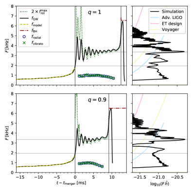
Figure 7: Left panels: time evolution of GW frequency $f_{\mathrm{GW}}$, maximum rotation rate $\nu_{\mathrm{max}}$, radial oscillation frequency $f_{\mathrm{radial}}$, and the rate of the modulation of the GW frequency, $f_{\mathrm{vibrato}}$. Vertical lines mark time of merger and apparent horizon formation. For comparison, we show the inspiral GW frequency $f_{\mathrm{model}}$ according to the IMRPhenomD_NRTidalv2 waveform model. Further, we compute the $m=l=2$ BH quasinormal-mode frequency $f_{\mathrm{BH}}$ from BH mass and angular momentum as found in the simulation at each time. Horizontal lines mark the frequency at merger (maximum GW amplitude) and the main peak of the spectrum. Right panels: Power spectrum of the $l=m=2$ component of the GW signal, at distance $40.7\usk\mathrm{M}\mathrm{Pc}$, in terms of $F\tilde{h}(F)$, where $\tilde{h}^{2}(F)=\tilde{h}_{+}^{2}(F)+\tilde{h}_{\times}^{2}(F)$. For comparison we show the design sensitivity curves for various detectors, taken from Evans et al. (2020).

III.3 Radial Remnant Profiles

We begin our discussion of the remnant structure with the average radial mass distribution shortly before the onset of collapse. For this we use the measure introduced in Sec. II.4. Fig. 8 shows the profile of baryonic mass contained within isodensity surfaces versus the proper volume within the same surfaces. We also mark the bulk region defined in Sec. II.4. As shown in Fig. 3, there is a smooth transition between remnant core and surrounding disk. This is also reflected in the mass-volume profile.

It is instructive to compare this profile to those obtained for nonrotating NS with same EOS as the initial data. In a previous work Kastaun et al. (2016), we introduced a method to find a nonrotating NS model (with same EOS as the initial data) for which the profile of the core resembles the one of the remnant. To this end, we compute the bulk mass versus bulk volume for the whole sequence of nonrotating NS and find the intersection with the remnant mass-volume profile, provided that it does intersect.

The sequence is shown in Fig. 8 and just barely intersects the remnant profile, near the maximum mass NS model. The figure also shows the mass-volume profile of the corresponding NS model, which we refer to as core-equivalent TOV model. It agrees remarkably well with the merger remnant profile within the whole bulk of the NS. Close to the NS surface, the two profiles naturally start to deviate, with the merger remnant profile smoothly extending to the debris disk.

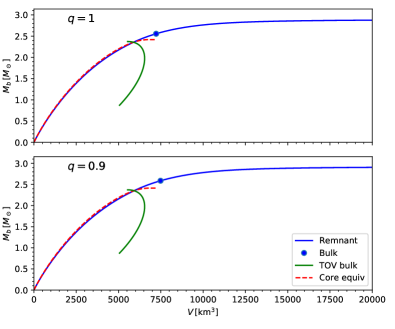
Figure 8: Total baryonic mass contained inside surfaces of constant density (blue curve) versus proper volume contained within the same surfaces. The top panel shows the remnant for the equal mass case, the bottom panel for the unequal mass system, both at a time $1\usk\mathrm{m}\mathrm{s}$ before apparent horizon formation. The dot marks bulk mass and bulk volume of the remnant (see text). For comparison, we show bulk mass versus bulk volume (green line) for the sequence of nonrotating NS following the same EOS as the BNS initial data, starting at mass $0.9\usk M_{\odot}$ up to the maximum bulk mass. The intersection with the remnant mass-volume curve defines the core equivalent TOV model, for which we show the mass-volume relation as well (dashed red curve).

The time evolution of the core equivalent mass is shown in Fig. 9, whereas the evolution of the bulk density is depicted in Fig. 2. We find large initial oscillations which are almost completely damped until collapse. Simultaneously with the damping, we also observe a drift towards larger equivalent core mass and larger bulk density.

At some point, the remnant bulk density exceeds the maximum bulk density of TOV solutions and also no core equivalent NS can be found anymore. Collapse sets in within less than $1\usk\mathrm{m}\mathrm{s}$ after this point. This behavior agrees well with earlier results Ciolfi et al. (2017); Endrizzi et al. (2018) obtained for different systems. The mounting number of simulation results without any counterexample adds weight to the conjecture that a HMNS collapses as soon as it does not allow for a core equivalent TOV model anymore.

It should however be mentioned that the above conjecture is disregarding brief violations due to oscillations. For the $q=1$ case, the core is slightly too compact to allow a stable TOV core equivalent for a very brief time already during the first oscillations after merger (this is hardly visible in the figure).

Currently, it is up to speculation if one should expect collapse when this limit is briefly exceeded dynamically. Our original conjecture for the collapse criterion is motivated by quasi-stationary systems. It is however worth noting an example where the limit was almost reached during the initial oscillations without any collapse, presented in Ciolfi et al. (2017). The mass of this model was known to be just below the estimated threshold for prompt collapse for the given EOS (APR4). It seems likely that the merger studied here is also very close to prompt collapse.

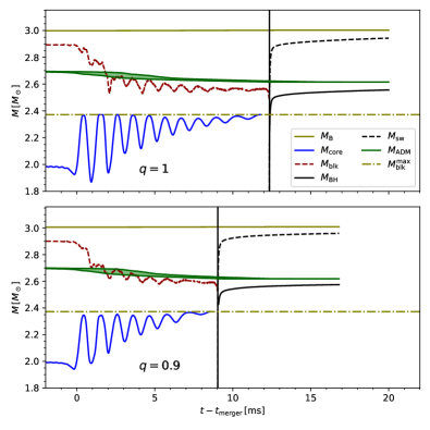
Figure 9: Evolution of masses for the equal mass case (top panel) and the unequal mass case (bottom panel). The dashed red curve shows the bulk baryonic mass, the solid blue curve the bulk baryonic mass of the core TOV equivalent (see main text), and the horizontal dash-dotted line the maximum bulk baryonic mass of nonrotating NS following the same EOS as the BNS initial data (SFHO). The solid black curve shows the gravitational mass of the BH (estimated from the apparent horizon) and the vertical line the time of first apparent horizon detection. The solid olive curve shows the total baryonic mass present in the computational domain up to BH formation, and a constant afterwards. The dashed black curve shows the baryonic mass swallowed by the BH. The green curve shows the ADM mass, where the shaded area is the contribution attributed to the energy of GW radiation within the computational domain.

Next, we turn to study the time evolution of the radial mass distribution. Since the average radial distribution in the late core is very close to the one of the maximum mass spherical NS, it is natural to subtract the latter. Fig. 10 shows the resulting differences in density profile in a time-radius diagram. As one can see, the deviations from the maximum mass TOV profile are larger at first, up to 60% of the maximum density, and also show large oscillations. A noteworthy property of the oscillations is that the density in the core does not significantly exceed the TOV model until shortly before collapse.

To further investigate the oscillations, we also show the volumetric radius of surfaces containing fixed amounts of baryonic mass in Fig. 10. The oscillation of the occupied proper volume provides a definition for an average radial displacement associated to those oscillations. Again, we see a strong damping of the oscillations.

In order to compute the frequency of the radial oscillation, we determine the maxima and minima of the bulk density shown in Fig. 2, after subtracting a quadratic fit to remove the drift. We then compute frequencies from the time between adjacent pairs of maxima as well as pairs of minima. The result is shown in Fig. 7. We find that the radial oscillation frequency decreases when approaching collapse.

We recall that for a nonrotating NS, collapse occurs when the square of the frequency of the radial quasinormal mode crosses zero. Under the assumption that the collapse mechanism for the merger remnant is the same, one would expect the radial oscillation frequency to approach zero as well. The evolution in Fig. 7 is compatible with this picture, although we cannot determine the oscillation frequency arbitrary close to the collapse (since we measure the oscillation frequency by distance between extrema).

Angular momentum conservation suggests that the radial oscillation should cause a modulation of the overall rotation, and therefore of the GW frequency. Indeed, the GW frequency shown in Fig. 7 shows minima and maxima that correlate with those of the bulk density. The modulation frequency obtained from minima and maxima of the GW frequency agrees very well with the radial oscillation frequency obtained from the density, and the modulation strength decreases with the radial oscillation amplitude.

As shown in Fig. 10, the volume occupied by isodensity surfaces containing fixed baryonic masses shows a slow decrease in the core. In this sense, the core is shrinking. Besides the core, Fig. 10 also shows the transition zone between remnant and disk. Here, the figure clearly shows an expansion of the isodensity surfaces of fixed mass. Even though the isodensity surfaces for the disk are not spherical anymore, our measure tells us that they occupy more space. This rules out mass accretion onto the remnant as a cause for the increasing compactness of the core.

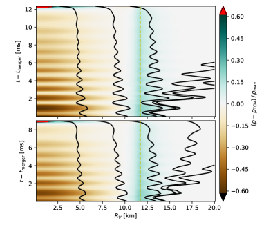
Figure 10: Evolution of radial mass distribution in the merger remnant for the equal mass case (top panel) and unequal mass case (bottom panel). The solid black curves show the time evolution of the proper volume within isodensity surfaces containing fractions $0.1,0.5,0.9,0.97$, and $0.98$ of the total baryonic mass. The volume is given in terms of volumetric radius $R_{V}$, the radius of an Euclidean sphere of equal volume. We further compare the remnant to the spherical NS solution of maximum bulk mass. For both, we compute the density as function of proper volume within isodensity surfaces. The color scale represents the difference of density at given volumetric radius, normalized to the maximum density of the spherical NS. The volumetric surface radius of the latter is shown as dashed vertical line.

III.4 Three-dimensional Remnant Structure

After studying the average radial mass distribution, we now turn to investigate the overall structure of the 3D fluid flow inside the remnant. Conceptually, we decompose the dynamics into a rotation with slowly drifting angular velocity, a quasi-stationary flow pattern, and subdominant contributions such as quasi-radial oscillations.

To extract the quasi-stationary part of the flow in the rotating frame, we employ a complex postprocessing chain as follows. First, we select a time window for averaging. For each of the 3D datasets saved during the simulation at regular intervals within the window, we first load 3D mesh-refined simulation data. This data is resampled onto a regular grid uniform in simulation coordinates that is covering the region of interest. Next, we apply the coordinate transformation into the corotating postprocessing coordinates described in Sec. II.3. During this step, we resample again onto a regular grid, this time uniform in the postprocessing coordinates. We also compute the Jacobian of the transformation in order to transform vectors correctly. To account for the time-dependent transformation of spatial coordinates, we further compute a new shift vector with the corresponding corrections. In this fashion, we compute the quasi-stationary density $\mathrm{bar}{\rho}$ and fluid velocity with respect to the corotating postprocessing coordinates, $\mathrm{bar}{w}^{i}$.

For visualization purposes, we compute the integral curves of the coordinate velocity $\mathrm{bar}{w}$. If the flow pattern were truly stationary, those curves would correspond to fluid trajectories. Because the structure is slowly changing and because we average out oscillations, the integral curves do not agree exactly with trajectories. That said, they do represent a good measure for the overall structure of the fluid movement.

Fig. 11 shows the integral curves together with two isodensity surfaces of $\mathrm{bar}{\rho}$ around $7\usk\mathrm{m}\mathrm{s}$ after merger for the unequal mass case. A prominent feature visible in the figure is the presence of two secondary vortices. Such vortices seem to be a generic feature, which we have observed in previous works Kastaun et al. (2016, 2017); Ciolfi et al. (2017) that studied the fluid flow within equatorial plane. The 3D results shown in Fig. 11 demonstrate how those vortices extend above and below the equatorial plane. We find that the direction of the fluid flow has negligible vertical components, except for the region within the secondary vortices. Even there, the absolute velocities are small. This suggests that mixing of matter in the vertical direction can probably by neglected.

The figure also shows that the inner fluid flow is still strongly non-axisymmetric. We recall that our coordinates are constructed such that a physically axisymmetric system would also appear axisymmetric in the postprocessing coordinates. The deformation of the fluid flow correlates with a strong elliptical deformation of the inner isodensity surface shown in the figure. The isodensity surface outside the secondary vortices is deformed less strongly, but exhibits some bumps which seem to be related to the secondary vortices.

Notably, the bumps in the outer regions are oriented nearly orthogonal to the deformation of the core. This is relevant for the GW signal, since the corresponding quadrupole moments in the rotating frame have different sign. The resulting GW signal is then the difference of two contributions. This might explain why numerical simulations sometimes exhibit pronounced secondary minima in the post-merger signal that are accompanied by a phase jump, as discussed in Kastaun et al. (2017). The relative amplitudes of the two contributions can change, which might result in a zero-crossing of the quadrupole moment in the rotating frame. We reserve the quantitative discussion of this effect for future work but point out that, even though the deformation of the outer regions seems less pronounced and is located in less dense regions, this might be compensated by the quadratic radial factor in the qudrupole moment and the cubic radial factor from the volumes involved.

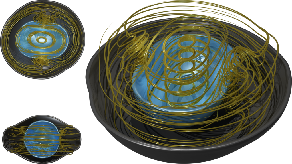
Figure 11: Quasi-stationary part of the remnant structure, in the frame corotating with $m=2$ density perturbation of remnant. The visualization represents the average over a time window $7\pm 1\usk\mathrm{m}\mathrm{s}$ after merger ($2\usk\mathrm{m}\mathrm{s}$ before collapse) for the $q=0.9$ case. The inner and outer surfaces (cut open) mark mass densities $0.3$ and $0.01$ of the maximum density, respectively. The wires represent integral lines of the averaged velocity field, shown inside the dense region enclosed within the outer surface. The top left rendering shows the remnant from a perspective along the rotation axis, the bottom left one from the side, along the longer axes of the deformed core, looking onto a meridional plane that cuts through the secondary vortices.

In Fig. 12, we compare the remnant structure at time shown in Fig. 11 to times shortly after merger and shortly before collapse. Although there are some differences, the non-axisymmetric deformation and the secondary vortices stay prominent right until collapse. This corresponds to a large GW amplitude sustained until collapse, which was shown in Sec. III.2.

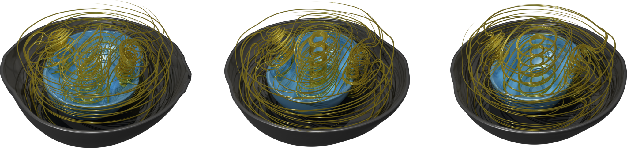
Figure 12: Remnant structure visualized as in Fig. 11, but for three different time windows. From left to right: $3\pm 1\usk\mathrm{m}\mathrm{s}$ after merger, $5\pm 1\usk\mathrm{m}\mathrm{s}$ after merger, and $7\pm 1\usk\mathrm{m}\mathrm{s}$ after merger ($2\usk\mathrm{m}\mathrm{s}$ before collapse). The camera distance remains constant to allow size comparison.

III.5 Differential Rotation

We now discuss the rotation profile of the remnant. Although the fluid flow is decidedly non-axisymmetic, it is instructive to study the axisymmetric part obtained by averaging in azimuthal direction. We start with the rotation profile in the equatorial plane. The azimuthal average with respect to the post-processing coordinates is depicted in Fig. 13. The profile shows the same generic behavior found for many different systems Ciolfi et al. (2017); Kastaun and Galeazzi (2015); Kastaun et al. (2016, 2017); Ciolfi et al. (2019); Endrizzi et al. (2018, 2016); Hanauske et al. (2017). The rotation of the core is comparatively slow with respect to infinity, and it is rotating very slowly with respect to the local inertial frame. Further out, the rotation rate exhibits a maximum.

As in previous works, we find that this maximum average rotation rate agrees well with half of the instantaneous GW frequency. This agreement has already been observed before Kastaun and Galeazzi (2015); Kastaun et al. (2016, 2017); Endrizzi et al. (2016); Ciolfi et al. (2017, 2019) and we are not aware of a counterexample. Although it is too early to generalize, the indications accumulate that this relation might be typical.

The evolution of maximum rotation rate and half the GW frequency is shown in Fig. 7. The frequencies do not just coincide at the time shown in Fig. 13. Clearly, they agree well throughout most of the post-merger phase. However, a few $\usk\mathrm{m}\mathrm{s}$ after the time $t_{\mathrm{merger}}$ of peak GW amplitude, the system is still in the process of merging. The computed maximum rotation rate is not meaningful during this period because during this phase it corresponds to the shear component near the origin. Consequently the correlation to the GW frequency is not present.

At larger radii, the rotation rate slowly approaches the Kepler rate as the remnant transitions into the disk. Since there still is a pressure gradient in the disk, the rotation is slightly slower than the orbital velocity. For comparison, we also plot the orbital velocity profile for the BH present shortly after collapse (mass and spin are given in Table 2). Naturally, it agrees well with the orbital velocity before collapse. Surprisingly, the orbital frequency of the innermost stable circular orbit agrees with the maximum rotation rate and half GW frequency before collapse. We are not aware of any reason this should be the case, and it might well be a numerical coincidence.

Fig. 13 also shows the radius and rotation rate for two sequences of uniformly rotating supramassive NS with same EOS as the initial data. One sequence is given by the models at mass shedding limit, and the other by models with the minimum angular momentum required to allow stable solutions. We find that the radius of the maximum mass model is very close to the innermost stable circular orbit of the final BH. We also observe a close match between the rotation rate of the maximum mass model and the maximum of the remnant rotation rate profile. This might be a coincidence. Nevertheless, it should be noted that such a relation would be extremely useful, since it would allow to predict the GW frequency of a HMNS directly before BH formation from the EOS alone, without even using the total mass of the system.

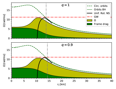
Figure 13: Rotation profile of the merger remnant $1\usk\mathrm{m}\mathrm{s}$ before collapse, for mass ratios $q=1$ and $q=0.9$. The filled curve shows the angular velocity (as seen from infinity) and the frame dragging contribution, in the equatorial plane versus circumferential radius. The data has been averaged in $\phi$-direction and over a time window $\pm 0.5\usk\mathrm{m}\mathrm{s}$. For comparison, we show the angular velocity of test particles in prograde circular orbit (dashed curve), and the same for particles orbiting the spinning BH formed after collapse (solid green curve). The solid black curves show the rotation rate and surface radius of uniformly rotating supramassive NS, either at mass shedding limit (right curve) or at minimal angular momentum (left curve). The vertical line marks the radius where the $\phi$-averaged mass density in the equatorial plane falls below 5% of the central value. The horizontal line marks half of the GW angular frequency.

We now turn to the rotation profile outside the equatorial plane. The left panel of Fig. 14 shows the azimuthal average of rotation rate as function of the distance $d$ to the $z$-axis and of the $z$-coordinate. The rotation rate is computed with respect to a straight rotation axis orthogonal to the equatorial plane. The centers of rotation on each plane parallel to the equatorial plane nearly coincide with this line, but do not form a perfectly straight line. This misalignment is visible in the plot as artifacts close to the axis, even though the underlying velocity field is smooth.

The rotation rate in the corotating postprocessing frame is mostly negative. The region with zero rotation in this frame corresponds to the maximum rotation rate in the inertial frame (compare Fig. 13). Inside the remnant core, we find that the profile mainly depends on $d$ and less on $z$. Along the axis, we also observe some differential rotation in $z$-direction outside the dense regions.

From the 3D visualization Fig. 11, we already know that the fluid flow shows pronounced deviations from axisymmetry. This can also be seen in the middle and right panels of Fig. 14. Those show the rotation rate in two meridional planes orthogonal to each other, one of which (right panel) is passing through the secondary vortices visible in Fig. 11.

The vortices themselves are stationary in the rotating postprocessing frame, and their own rotation is prograde with respect to the remnant. The local rotation rate (w.r.t. inertial frame) inside the vertices exceeds the rotation rate of the dominant density perturbation on the vertex side opposite to the remnant center. The meridional plane crossing the vortices exhibits stronger gradients of rotation rate than the orthogonal meridional plane shown in the middle panel.

The local deviation of the flow from axisymmetry correlates with a nonaxisymmetric perturbation of the density. This can be seen in the overlaid isodensity contours in Fig. 14. The right panel depicting the cut through the vortices shows a slightly prolate core. Further out, the isodensity contours are not simple ellipsoids but exhibit an equatorial bump. In contrast, the same density contour in the middle panel is nearly ellipsoidal and the core is slightly oblate.

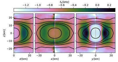
Figure 14: Twodimensional differential rotation profile of the remnant for mass ratio $q=0.9$, averaged over the time window $7\pm 1\usk\mathrm{m}\mathrm{s}$ after merger. The color scale denotes the rotational frequency in the coordinate system corotating with the perturbation pattern. Negative values signify that (in the inertial frame) the fluid is rotating more slowly than the pattern. The left panel shows the average in $\phi$-direction versus cylindrical radius and z-coordinate. The right panel shows a cut in $(y,z)$-plane, the $y$-axis being roughly aligned with the secondary vortices shown in Fig. 11. The middle panel shows the $(x,z)$-plane instead. The solid curves mark isodensity contours (in the left panel with respect to $\phi$-averaged density). Radial distances in the equatorial plane and distances along the z-axis are both proper distances, allowing to asses the oblateness of the remnant.

III.6 Disk Vorticity

Besides the fluid flow inside the hypermassive NS, we are also interested in the dynamics of the surrounding disk. As already shown in Fig. 1, the disk is subject to continuous strong perturbations until the BH is formed. We have also shown in Fig. 10 that matter migrates from the NS into the disk. One can therefore expect an impact on the fluid flow, causing deviations from a quasi-Keplerian disk.

The velocity field in the disk is dominated by the quasi-Keplerian velocity profile shown in Fig. 13. In order to get a more detailed picture, we compute the fluid vorticity in three dimensions, which, being a differential expression, is more sensitive to local deviations. We recall that the most appropriate vorticity measure in the relativistic case is given by $\partial_{i}(hv_{j})-\partial_{j}(hv_{i})$. However, since metric and enthalpy are not saved as 3D data in our simulations, we instead compute the ordinary curl $\vec{\nabla}\times\vec{w}$, where $w^{i}=\alpha v^{i}-\beta^{i}$ is the fluid advection speed with respect to the simulation coordinates, and $\vec{\nabla}$ refers to the ordinary partial derivatives. We also do not use our usual postprocessing coordinates because they are not available after BH formation. This simple vorticity measure is sufficient for the following qualitative discussion of local shear, but not suitable for a study of vorticity conservation.

For visualization purposes, we compute integral curves of the instantaneous vorticity. We do not average the velocity field in time, because here the focus is on the impact of disturbances, not on the overall average fluid flow. The result is shown in Fig. 15. We find that the vorticity field is quite irregular outside the NS. Using an interactive rendering of the figure, we observed many closed vorticity lines, similar to those found in smoke rings. Our cursory visual inspection did not reveal any linked loops. Overall, the non-radial components dominate the vorticity.

Comparing the disk before and after merger, we observe that the density quickly becomes more axisymmetric after the NS collapses, as it ceases to inject spiral waves into the disk. This can also be seen in Fig. 1. The vorticity structure on the other hand does not become regular, i.e., the numerous small-scale vortices continue to dominate the local shear until the end of the simulation.

Our findings suggest a possible interpretation as follows. The rotating non-axisymmetric deformation and the radial oscillations inject a complicated pattern of waves into the disk that stir up the matter. The resulting perturbations dominate the vorticity on medium and small length scales. As long as vorticity is conserved (which is not necessarily the case in hot matter and also not expected to hold exactly when using the curl as vorticity measure) one can expect the disturbances to manifest as closed vorticity lines. Since vorticity lines are dragged along the fluid, the differential rotation of the disk stretches small vorticity loops, resulting in a predominantly non-radial orientation. Another possible interpretation would be turbulence.

Whether the fluid is turbulent in the strict fluid dynamics sense or just exhibits a very irregular looking flow, our results suggest that treating the flow inside the disk as laminar might not be sufficient for all applications. Most notably, properties of the MRI instability are often predicted in terms of rotation rate around the origin, density, and magnetic field strength. However, since the local shear is dominated by essentially random and time-dependent perturbations, this might not be justified. On the other hand, a magnetic field of sufficient strength might have a dampening impact on local vortices.

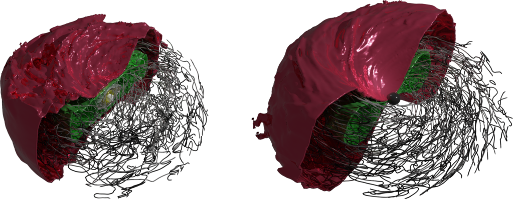
Figure 15: Vorticity lines inside the disk $2\usk\mathrm{m}\mathrm{s}$ before (left) and $5\usk\mathrm{m}\mathrm{s}$ after BH formation (right), for the $q=0.9$ case. The black surface in the right panel marks the apparent horizon. The cut-open solid surfaces in the left panel mark densities $4.0\times 10^{10},2.2\times 10^{11},1.7\times 10^{13}$, and $5.0\times 10^{14}\usk\mathrm{g}\mathrm{/}\mathrm{c}\mathrm{m}\mathrm{{}^{3}}$, in the right panel $1.5\times 10^{10}$ and $8.1\times 10^{10}\usk\mathrm{g}\mathrm{/}\mathrm{c}\mathrm{m}\mathrm{{}^{3}}$. Vortex lines are cut off outside the outermost surface and beyond a length cutoff in order to limit cluttering. The color indicates the vorticity magnitude, where lighter color corresponds to larger values. The camera distance is the same in both panels.

III.7 Angular Momentum and Energy

We now discuss the distribution of mass and angular momentum using the various measures discussed in Sec. II.4. Our main interest is whether the remnant collapses because of angular momentum transport within the fluid or because of angular momentum loss via GW radiation. We will answer this for the numerical results, but emphasize that angular momentum transport is most likely not captured correctly. The lack of effective magnetic viscosity might lead to underestimation of the dissipation of differential rotation, while the unavoidable numerical viscosity might lead to overestimation in case of low actual viscosity.

First, we establish how much angular momentum and energy is lost via GW. The total ADM energy is shown in Fig. 16 as function of total angular momentum. We mark the values at merger and collapse to visualize the loss during the post-merger phase (the BH ringdown is negligible). However, it would be wrong to directly associate this loss to the changes in the remnant, for the following reason. At the time when the merger signal reaches the extraction radius, the space between remnant and extraction radius contains strong GW radiation from the early post-merger phase (compare Fig. 9). We find that the radiated energy and angular momentum corresponding to this part of the signal constitutes a significant fraction of the total loss. To get a better handle on the energetics of the remnant, we computed the total energy and angular momentum at times when the wavefront passing a smaller sphere at time of merger reaches the extraction radius. In the same way, we treat the time of collapse. This is similar to using a small extraction radius, but avoids extracting GW in the strong field zone. The resulting values for energy and angular momentum, which are also shown in Fig. 16, should be more closely related to the changes within the remnant. We therefore think of those as energy and angular momentum of the remnant and disk.

For comparison, Fig. 16 also shows the ranges possible for uniformly rotating NS with the initial data EOS, as well as the curve for critical Kerr BH. Clearly, both the total energy and the total angular momentum of remnant and disk (see above) are always larger than the maximum values for uniformly rotating NS. For the energy, this can be expected since the total baryonic mass is in the hypermassive range. The comparison to the Kerr curve shows that energy and angular momentum of remnant and disk could be realized by a BH at any time.

The actual values for the final BH are shown in Fig. 16 as well. The BH energy and angular momentum shown are computed using the isolated horizon framework and would correspond to the ADM values for an isolated BH. However, the final BH is still surrounded by a massive disk, which accounts for the difference to the total ADM energy and angular momentum in the computational domain. The figure also contains the values shortly after BH formation. The differences to the final values are mainly due to matter not in stable orbits falling in during the first few $\mathrm{m}\mathrm{s}$. The early BH is interesting because it corresponds more closely to the part that actually collapsed.

In order to get an estimate of the angular momentum transport inside the remnant, we study the integrands of the ADM volume integrals. At each time, we compute the contributions to ADM energy and angular momentum integrals within coordinate spheres as function of the sphere’s coordinate radius. Fig. 16 shows the resulting curves at 5 different times. In addition, we show the time evolution for coordinate spheres with time-dependent radius chosen such that the baryonic mass within the radius stays constant. The time evolution of angular momentum and energy within those spheres is thus proportional to the average angular momentum and energy per baryonic mass. The largest radius plotted is the one of the sphere that contains exactly the amount of baryonic mass that is swallowed by the BH within $1\mathrm{m}\mathrm{s}$ of apparent horizon formation (but not exactly the same matter, as the swallowed region is non-spherical).

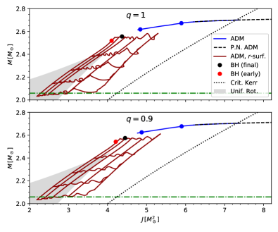
Figure 16: Evolution of energy and angular momentum for the equal mass system (top panel) and the $q=0.9$ case (bottom panel). The solid blue curve shows total ADM energy versus angular momentum, and the dashed black line a post-Newtonian approximation for the inspiral of point particles. The blue circles represent energy and angular momentum excluding the amount attributed to GW radiation outside $r=100\usk\mathrm{k}\mathrm{m}$, at times $1\usk\mathrm{m}\mathrm{s}$ after merger and $1\usk\mathrm{m}\mathrm{s}$ before collapse. The black and red dots mark energy and angular momentum of the BH at the end of the simulation and $1\usk\mathrm{m}\mathrm{s}$ after apparent horizon formation. The diagonally oriented red curves show the contributions within spheres of constant radius to the ADM volume integrals, at regular intervals from $1\usk\mathrm{m}\mathrm{s}$ after merger to $1\usk\mathrm{m}\mathrm{s}$ before apparent horizon formation. The horizontally oriented red curves show the time evolution of the contributions within spheres containing different fixed amounts of baryonic mass, ranging from $2.5\usk M_{\odot}$ up to the baryonic mass swallowed by the BH within $1\usk\mathrm{m}\mathrm{s}$ after formation. The shaded region is bounded by the mass shedding limit and smallest possible angular momentum of stable uniformly rotating NSs. The green horizontal line marks the maximum mass of nonrotating NS. The dotted line shows the angular momentum of critical Kerr BHs.

From the shape of the resulting grid, we deduce that the angular momentum loss dominates the angular momentum redistribution within the remnant. Furthermore, the angular momentum loss of the remnant is comparable to the loss by GW. Fig. 16 in conjunction with our finding that matter is migrating outwards into the disk, as shown in Fig. 10, suggests that the associated angular momentum transport is subdominant to the GW in this case.

We recall that the integrands in the ADM volume integrals are gauge dependent quantities that depend on the time slicing. The use of coordinate spheres we used above also introduce a dependence on the spatial coordinates used in the simulation. It is therefore advisable to compare with other measures.

One comparison we can do is between the ADM angular momentum and an approximation of Komar angular momentum (see Sec. II.4). The latter is dependent on the spatial gauge as well but in a different manner. The comparison might reveal gauge dependencies of the results, but an agreement is no conclusive proof that gauge effects are negligible. The two measures are shown in Fig. 17 for the time shortly before collapse. We find that the Komar-type angular momentum measure matches the ADM angular momentum almost exactly, as would be expected for an axisymmetric spacetime.

Another simple comparison is between the ADM quantities computed within coordinate spheres and those computed within the isosurfaces of mass density. The latter surfaces are independent on the spatial gauge. Although the density distribution is not spherically symmetric, we find that the two measures match well. Our comparisons indicate that the qualitative picture we derived from Fig. 16 is not simply an artifact of gauge effects.

For comparison, Fig. 17 also shows the allowed region for uniformly rotating NS. Somewhat surprisingly, the remnant profile passes right through the uniformly rotating model of maximum mass. We are unaware of a reason to expect such behavior, which might well be a numerical coincidence.

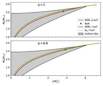
Figure 17: Distribution of angular momentum at time $1\usk\mathrm{m}\mathrm{s}$ before collapse for the equal mass system (top panel) and the $q=0.9$ case (bottom panel). The solid red curve shows the contribution to the ADM angular momentum within isodensity surfaces as function of the baryonic mass within the same surfaces. The green dot marks the position of the remnant bulk (see main text). The solid green line shows the same for spherical surfaces (spherical with respect to simulation coordinates). It is hidden behind the dashed yellow curve, which shows an estimate of the Komar angular momentum (see text). The shaded area shows the values possible for uniformly rotating NS.

We are lead to the conclusion that the remnant studied in our simulations is driven to collapse mainly by angular momentum loss via GW, whereas angular momentum transport into the disk or within the remnant are less important factors. We stress that our findings do not necessarily generalize to all HMNS. For even longer lived remnants, the angular momentum transport can definitely become more important, as was shown in Nedora et al. (2021).

IV Summary

In this work we present a possible scenario for the fate of the merger remnant of GW170817. We employ standard numerical simulation techniques and focus on the most fundamental hydrodynamic processes, ignoring magnetic fields and neutrino radiation. The main motivation is a better qualitative understanding of hypermassive merger remnants. To this end, we create novel postprocessing and visualization tools to analyze the numerical results. Those methods provide a more detailed view on three key aspects of the simulated mergers.

First, we find that the merger remnants are not merely differentially rotating axisymmetric systems deformed by some oscillation modes known from linear perturbation theory. The flow and the density deformation are best described in a rotating frame, where they form a pattern that remains stable until the remnant collapses to a BH. A prominent feature of the flow pattern are secondary vortices in the outer layers. Such vortices were already observed in earlier studies restricted to the equatorial plane. Here, we visualized how they extend outside the equatorial plane. The density deformation pattern in the aforementioned rotating frame is not a simple ellipsoidal deformation either. Instead, we find that the perturbation in the core is oriented nearly orthogonal with respect to the deformation near the transition zone to the disk. The latter deformation seems related to the secondary vortices which are located at radii between the two regimes.

The deformation of the remnant is directly related to the GW signal. As in earlier studies, we find that the GW frequency is twice the maximum rotation rate. The maximum rotation rate is modulated by a decaying quasi-radial oscillation, which matches exactly a modulation of the GW frequency. Another noteworthy aspect is that the spatial phase-shifts mentioned above imply cancellation effects in the quadrupole moment, and therefore the GW amplitude. Moreover, the shape of the deformation undergoes a slow drift, such that cancellation effects become time-dependent.

One may speculate whether this effect can become pronounced enough to cause zero-crossings of the quadrupole moment in the rotating frame. Such crossings would explain secondary minima and phase jumps in addition to those occurring during merger, which are sometimes observed in numerical simulations of post-merger GW signals. For the examples studied here, no secondary phase jumps were observed, however.

Second, we find at any time that the overall radial mass distribution in the remnant core is well approximated by profiles of a nonrotating isolated NSs. This fits well to the relatively slow rotation rate in the core, as was already observed in many earlier works. A key observation is that the profile directly before the onset of collapse matches the profile in the core of the maximum mass nonrotating NS. In earlier work we proposed that, for generic hypermassive remants, collapse sets in exactly when the core reaches this critical density profile, which depends only on the EOS. The new examples add further support to this conjecture.

Third, we identify the mechanism responsible for the drift of the density profile leading towards the eventual collapse. By studying the radial distributions of mass and angular momentum and their time evolution, we rule out a change in differential rotation inside the remnant as dominant cause. We also rule out angular momentum transfer into the disk and accretion onto the remnant. Instead, the main effect is the angular momentum carried away by the strong GW emitted until collapse.

We have to stress, however, that small scale magnetic field amplification effects, which are not taken into account in our simulations, might lead to a large effective viscosity. This might speed up the loss of differential rotation to a degree such that it becomes dominant over the impact of angular momentum loss via GW. Nevertheless, considering only the latter in a simulation provides an upper limit for the collapse delay that does not depend on effective viscosity. We emphasize that the above statements refer to the systems studied here, which form a hypermassive NS that emits a strong GW signal and collapses within tens of milliseconds. Our results cannot be generalized to longer-lived remnants, which are not ruled out by the observational data for GW170817.

Another avenue for future research is the impact of neutrino radiation transport on the non-axisymmetry of the remnant. As in earlier work, we find a non-axisymmetric thermal structure that corotates with the overall flow pattern. It is unknown how important the corresponding thermal pressure perturbations are for maintaining the non-axisymmetric remnant perturbation. Since the latter are the cause of the post-merger GW signal, one can speculate on a relation between neutrino cooling and the decay of the GW amplitude.

Last but not least, we investigate the disk surrounding the remnant and matter ejected from the system. The mass of the disk present in our simulation after BH formation is sufficient to allow the massive wind component (red component) inferred from kilonova AT2017gfo, although this would require an efficient mechanism for expelling matter. The dynamical mass ejection in our results is insufficient to explain the blue component inferred from the kilonova.

Making conclusive statements on the compatibility of our models with AT2017gfo, however, would require a convergence study with much higher resolutions. In fact, there is some tension with published results evolving our equal-mass model, including also neutrino radiation. This study does carry out a resolution test, but could not prove convergence of ejecta and disk masses for the model studied here either. Those simulations predict less dynamical ejecta and less massive disks. Noteworthy, they also result in shorter lifetimes of the HMNS.

In our case, we find that matter is migrating into the disk from the HMNS, a result we also found in earlier work of different systems. This effect might further increase when taking into account magnetically driven winds from the HMNS remnant. We also find that the HMNS is strongly perturbing the disk, which apparently causes part of the disk to become unbound. For the cases at hand, the tidal ejection during merger is insignificant in comparison.

The above observations suggests that the lifetime of the HMNS remnant — which is extremely sensitive to the total mass and to numerical errors because the system is close to collapse — is indeed one of the main uncertainties regarding disk mass and mass ejection. It could prove difficult to find analytic fits to the parameters of the binary, and it might be advisable to treat the lifetime of HMNS as a free (albeit constrained) parameter in such fits.

The perturbation of the disk by the HMNS also has an effect on the velocity field in the disk, as shown by novel 3D visualizations of the vorticity field both before and after BH formation. We observe an irregular vorticity field instead of the ordered structure that would be present for a Keplerian velocity profile. This indicates that the shear on medium length scales is dominated by the disturbances originating from the remnant.

The irregular vorticity structure is relevant with regard to estimates for the time and length scales of magneto-rotational instabilities, because the analytic models used for such predictions are based on disks with an orderly flow. Although the density perturbations quickly settle down after BH formation, we find that the vorticity remains irregular until the end of the simulation.

In this work, we focused on two examples only and refrained from costly high-resolution studies. Those two examples paint a qualitative picture of the HMNS structure and evolution. As a future step, the analysis developed in this work needs to be applied to more simulations in order to determine which parts of this picture are generic. This will also benefit the development of more realistic models for HMNS created in mergers. Such models are needed for the analysis of future GW detections of a post-merger signal, as performing a large number of brute force merger simulations is computationally too expensive. As qualitative examples for calibrating such models, we provide the GW data from our simulations.