Contextually Guided Convolutional Neural Networks for Learning Most Transferable Representations

Abstract

Deep Convolutional Neural Networks (CNNs), trained extensively on very large labeled datasets, learn to recognize inferentially powerful features in their input patterns and represent efficiently their objective content. Such objectivity of their internal representations enables deep CNNs to readily transfer and successfully apply these representations to new classification tasks. Deep CNNs develop their internal representations through a challenging process of error backpropagation-based supervised training. In contrast, deep neural networks of the cerebral cortex develop their even more powerful internal representations in an unsupervised process, apparently guided at a local level by contextual information. Implementing such local contextual guidance principles in a single-layer CNN architecture, we propose an efficient algorithm for developing broad-purpose representations (i.e., representations transferable to new tasks without additional training) in shallow CNNs trained on limited-size datasets. A contextually guided CNN (CG-CNN) is trained on groups of neighboring image patches picked at random image locations in the dataset. Such neighboring patches are likely to have a common context and therefore are treated for the purposes of training as belonging to the same class. Across multiple iterations of such training on different context-sharing groups of image patches, CNN features that are optimized in one iteration are then transferred to the next iteration for further optimization, etc. In this process, CNN features acquire higher pluripotency, or inferential utility for any arbitrary classification task, which we quantify as a transfer utility. In our application to natural images, we find that CG-CNN features show the same, if not higher, transfer utility and classification accuracy as comparable transferable features in the first CNN layer of the well-known deep networks AlexNet, ResNet, and GoogLeNet. In general, the CG-CNN approach to development of pluripotent/transferable features can be applied to any type of data, besides imaging, that exhibit significant contextual regularities. Furthermore, rather than being trained on raw data, a CG-CNN can be trained on the outputs of another CG-CNN with already developed pluripotent features, thus using those features as building blocks for forming more descriptive higher-order features. Multi-layered CG-CNNs, comparable to current deep networks, can be built through such consecutive training of each layer.

Keywords— Deep Learning, Contextual Guidance, Unsupervised Learning, Transfer Learning, Feature Extraction, Pluripotency.

1 Introduction

Deep learning approach has led to great excitement and success in AI in recent years LeCun et al., (2015); Krizhevsky et al., (2012); Zhao et al., (2019); Marblestone et al., (2016); Goodfellow et al., (2016); Ravi et al., (2017). With the advances in computing power, the availability of manually labeled large data sets, and a number of incremental technical improvements, deep learning has become an important tool for machine learning involving big data Zhao et al., (2019); Marblestone et al., (2016); Goodfellow et al., (2016); Gao et al., (2020); Poggio, (2016). Deep Convolutional Neural Networks (CNNs), organized in series of layers of computational units, use local-to-global pyramidal architecture to extract progressively more sophisticated features in the higher layers based on the features extracted in the lower ones Zhao et al., (2019); Goodfellow et al., (2016). Such incrementally built-up features underlie the remarkable performance capabilities of deep CNNs.

When deep CNNs are trained on gigantic datasets to classify millions of images into thousands of classes, the features extracted by the intermediate hidden layers – as opposed to either the raw input variables or the task-specific complex features of the highest layers – come to represent efficiently the objective content of the images Gao et al., (2020); Caruana, (1995); Bengio, (2012). Such objectively significant and thus inferentially powerful features can be used not only in the classification task for which they were developed, but in other similar classification tasks as well. In fact, having such features can reduce complexity of learning new pattern recognition tasks Phillips et al., (1995); Clark & Thornton, (1997); Favorov & Ryder, (2004). Indeed, taking advantage of this in the process known as transfer learning Gao et al., (2020); Thrun & Pratt, (2012); Pan et al., (2010); Yosinski et al., (2014), such broad-purpose features are used to preprocess the raw input data and boost the efficiency and accuracy of special-purpose machine learning classifiers trained on smaller datasets Zhao et al., (2019); Goodfellow et al., (2016); Yosinski et al., (2014); Bengio, (2012). Transfer learning is accomplished by first training a “base” broad-purpose network on a big-data task and then transferring the learned features/weights to a special-purpose “target” network trained on new classes of a generally smaller “target” dataset Yosinski et al., (2014).

Learning generalizable representations is improved with data augmentation, by incorporating variations of the training set images using predefined transformations Shorten & Khoshgoftaar, (2019). Feature invariances, which have long been known to be important for regularization Becker & Hinton, (1992); Hawkins & Blakeslee, (2004), can also be promoted by such means as mutual information maximization Becker & Hinton, (1992); Hjelm et al., (2019); Favorov & Ryder, (2004), or by penalizing the derivative of the output with respect to the magnitude of the transformations to incorporate a priori information about the invariances Simard et al., (1992), or by creating auxiliary tasks for unlabeled data Ghaderi & Athitsos, (2016); Dosovitskiy et al., (2014); Grandvalet & Bengio, (2004); Ahmed et al., (2008).

Although supervised deep CNNs are good at extracting pluripotent inferentially powerful transferable features, they require big labeled datasets with detailed external training supervision. Also, the backpropagation of the error all the way down to early layers can be problematic as the error signal weakens (a phenomenon known as the gradient vanishing Arjovsky & Bottou, (2017)). To avoid these difficulties, in this paper we describe a self-supervised approach for learning pluripotent transferable features in a single CNN layer without reliance on feedback from higher layers and without a need for big labeled datasets. We demonstrate the use of this approach on two examples of a single CNN layer trained first on natural RGB images and then on hyperspectral images.

Of course, there is a limit to sophistication of features that can be developed on raw input patterns by a single CNN layer. However, more complex and descriptive pluripotent features can be built by stacking multiple CNN layers, each layer developed in its turn by using our proposed approach on the outputs of the preceding layer(s).

In Section 2, we briefly review deep learning, transfer learning, and neurocomputational antecedents of our unsupervised feature extraction approach. In Section 3, we present the proposed Contextually Guided CNN (CG-CNN) method and a measure of its transfer utility. We present experimental results in Section 4 and conclude the paper in Section 5. An early exploration of CG-CNN has been reported in conference proceedings Kursun & Favorov, (2019).

2 Transferable Features at the Intersection of Deep Learning and Neuroscience

2.1 Transfer of Pluripotent Features in Deep CNNs

Deep CNNs apply successive layers of convolution (Conv) operations, each of which is followed by nonlinear functions such as the sigmoidal or ReLU activation functions and/or max-pooling. These successive nonlinear transformations help the network extract gradually more nonlinear and more inferential features. Besides their extraordinary classification accuracy on very large datasets, the deep learning approaches have received attention due to the fact that the features extracted in their first layers have properties similar to those extracted by real neurons in the primary visual cortex (V1). Discovering features with these types of receptive fields are now expected to the degree that obtaining anything else causes suspicion of poorly chosen hyperparameters or a software bug Yosinski et al., (2014).

Pluripotent features developed in deep CNN layers on large datasets can be used in new classification tasks to preprocess the raw input data to boost the accuracy of the machine learning classifier Gao et al., (2020); Thrun & Pratt, (2012); Pan et al., (2010). That is, a base network is first trained on a “base” task (typically with a big dataset), then the learned features/weights are transferred to a second network to be utilized for learning to classify a “target” dataset Yosinski et al., (2014). The learning task of the target network can be a new classification problem with different classes. The base network’s pluripotent features will be most useful when the target task does not come with a large training dataset. When the target dataset is significantly smaller than the base dataset, transfer learning serves as a powerful tool for learning to generalize without overfitting.

The transferred layers/weights can be updated by the second network (starting from a good initial configuration supplied by the base network) to reach more discriminatory features for the target task; or the transferred features may be kept fixed (transferred weights can be frozen) and used as a form of preprocessing. The transfer is expected to be most advantageous when the features transferred are pluripotent ones; in other words, suitable for both base and target tasks. The target network will have a new output layer for learning the new classification task with the new class labels; this final output layer typically uses softmax to choose the class with the highest posterior probability.

2.2 Pluripotent Feature Extraction in the Cerebral Cortex

Similar to deep CNNs, cortical areas making up the sensory cortex are organized in a modular and hierarchical architecture Hawkins et al., (2017); Marblestone et al., (2016). Column-shaped modules (referred to as columns) making up a cortical area work in parallel performing information processing that resembles a convolutional block (convolution, rectification, and pooling) of a deep CNN. Each column of a higher-level cortical area builds its more complex features using as input the features of a local set of columns in the lower-level cortical area. Thus, as we go into higher areas these features become increasingly more global and nonlinear, and thus more descriptive Clark & Thornton, (1997); Favorov & Ryder, (2004); Favorov & Kursun, (2011); Grill-Spector & Malach, (2004); Hawkins et al., (2017).

Unlike deep CNNs, cortical areas do not rely on error backpropagation for learning what features should be extracted by their neurons. Instead, cortical areas rely on some local guiding information in optimizing their feature selection. While local, such guiding information nevertheless promotes feature selection that enables insightful perception and successful behavior. The prevailing consensus in theoretical neuroscience is that such local guidance comes from the spatial and temporal context in which selected features occur Kursun & Favorov, (2019); Becker & Hinton, (1992); Favorov & Ryder, (2004); Körding & König, (2000); Phillips & Singer, (1997); Hawkins et al., (2017). The reason why contextually selected features turn out to be behaviorally useful is because they are chosen for being predictably related to other such features extracted from non-overlapping sensory inputs and this means that they capture the orderly causal dependencies in the outside world origins of these features Kay & Phillips, (2011); Phillips et al., (1995); Clark & Thornton, (1997); Hawkins et al., (2017); Favorov & Ryder, (2004); Becker & Hinton, (1992); Kursun & Favorov, (2019).

3 Contextually Guided Convolutional Neural Network (CG-CNN)

3.1 Basic Design

In this paper we apply the cortical context-guided strategy of developing pluripotent features in individual cortical areas to individual CNN layers. To explain our approach, suppose we want to develop pluripotent features in a particular CNN layer (performing convolution + ReLU + pooling) on a given dataset of images. We set up a three-layer training system (Fig. 1-A) as:

1. The Input layer, which might correspond to a 2-dimensional field of raw pixels (i.e., a 3D tensor with two axes specifying row and column and one axis for the color channels) or the 3D tensor that was outputed by the preceding CNN layer with already developed features;

2. The CNN layer (“Feature Generator”), whose features we aim to develop;

3. The Classifier layer, a set of linear units fully connected with the output units of the CNN layer, each unit (with softmax activation) representing one of the training classes in the input patterns.

As in standard CNNs, during this network’s training the classification errors will be backpropagated and used to adjust connection weights in the Classifier layer and the CNN layer.

While eventually (after its training) this CNN layer might be used as a part of a deep CNN to discriminate some particular application-specific classes of input patterns, during the training period the class labels will have to be assigned to the training input patterns internally; i.e., without any outside supervision. Adopting the cortical contextual guidance strategy, we can create a training class by picking at random a set of neighboring window patches in one of database images (Fig. 1-B). Being close together or even overlapping, such patches will have a high chance of showing the same object and those that do will share something in common (i.e., the same context). Other randomly chosen locations in the dataset images – giving us other training classes – will likely come from other objects and at those locations the neighboring window patches will have some other contexts to share. We can thus create a training dataset $\mathbf{X}=\{x^{t}\mid 1\leq t\leq CN\}$ of $C\times N$ class-labeled input patterns by treating $C$ sets of $N$ neighboring window patches – each set drawn from a different randomly picked image location – as belonging to $C$ training classes, uniquely labeled from 1 to $C$. These inputs are small $a\times a\times b$ tensors, $a\times a$ patches (feature-maps) with $b$ features. We will refer to each such class of neighboring image patches as a “contextual group.”

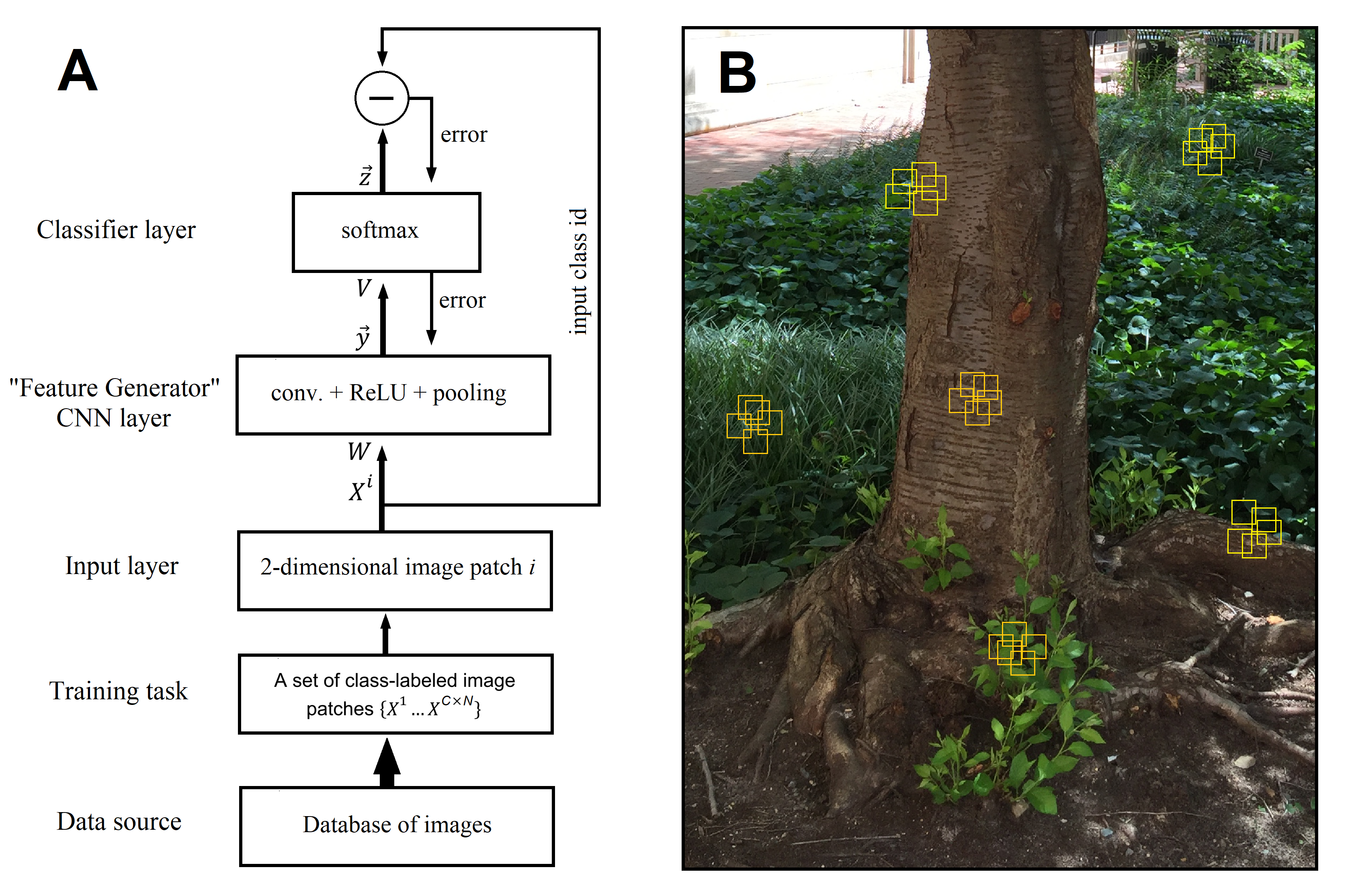
Fig. 1: Contextually Guided Convolutional Neural Network (CG-CNN) design. (A) CG-CNN architecture. (B) Class-defining contextual groups of image patches. Each image patch – used as input in CG-CNN training – is shown as a small square box superimposed on one of the database images. Neighboring patches constitute a contextual group and during network training are treated as belonging to the same class. During network training, locations of contextual groups are picked at random. Six such groups, or classes, are shown on this photo with five patches in each ($C=6$ and $N=5$).

Upon a presentation of a particular input pattern $x^{t}$ from the training dataset $\mathbf{X}$, the response of the CNN layer is computed as:

$$y_{j}^{t}=MaxPool([W_{j}*x^{t}]^{+})$$ (1)

where $y_{j}^{t}$ is the response of output unit $j$ in the CNN layer with $d$ units (i.e., $y_{j}$ is CNN’s feature $j$, where $1\leq j\leq d$), $W_{j}$ is the input connection weights of that unit (each unit has $w\times w\times b$ input connections), symbol * denotes convolution operation, and $[\makebox[3.87498pt]{{$\cdot$}}]^{+}=\max\{\makebox[3.87498pt]{{$\cdot$}},0\}$ denotes the ReLU operation. Next, the response of the Classifier layer is computed by the softmax operation as:

$$z_{l}^{t}=\frac{\exp{(V_{l}\boldsymbol{\cdot}y^{t})}}{\sum_{c=1}^{C}\exp{(V_{c}\boldsymbol{\cdot}y^{t})}}$$ (2)

where $z_{l}^{t}$ is the response of output unit $l$ in the Classifier layer (expressing the probability of this input pattern $x^{t}$ belonging to class $l$), $y^{t}=[y_{j}^{t}]_{j=1}^{d}$ is the $d$-dimensional feature vector computed as the output of the CNN layer, and $V_{l}$ is the vector of connection weights of that unit from all the $d$ units of the CNN layer.

During training, connection weights $W$ and $V$ are adjusted by error backpropagation so as to maximize the log-likelihood (whose negative is the loss function):

$$\mathcal{L}\big{(}V,W\big{|}\mathbf{X}\big{)}=\sum_{t=1}^{CN}{\sum_{c=1}^{C}r_{c}^{t}\log z_{c}^{t}}$$ (3)

where $r_{c}^{t}\in{0,1}$ indicates whether input pattern $x^{t}$ belongs to class $c$.

The nomenclature given below lists (in alphabetical order) and briefly describes several symbols that we use in our description of the CG-CNN algorithm.

List of Symbols

Symbol	Description
$a$	the width of the input image patches
$A_{CG}(C)$	transferable classification accuracy
$b$	the number of channels (e.g., red-green-blue) of the input image patches
$C$	the number of contextual groups
$d$	the number of feature maps (the features extracted from the $a\times a\times b$ input tensor and fed to the Classifier)
$g$	the extent of the spatial translation within contextual groups
$N$	the number of randomly chosen image patches in each contextual group
$r^{t}$	one-hot vector for the class label of $x^{t}$, where $r_{c}^{t}=1$ if and only if $x^{t}$ belongs to contextual group $c$
$s$	the stride of the convolutions
$U$	Transfer Utility, which is used to estimate the pluripotency of the learned convolutional features
$V_{l}$	softmax weights of Layer-5 for contextual group $l\in\{1,2,\dots,C\}$ for the current task of discriminating $C$ groups (each softmax unit has $d$ input connections coming from $y$)
$w$	the kernel size of the convolutions
$W_{j}$	convolutional weights of unit $j$ in Layer-2 (each unit/feature has $w\times w\times b$ input connections)
$x^{t}$	image patch number $t$ used as input to CG-CNN
$\mathbf{X_{E}}$	the training dataset formed by $x^{t}$ image patches ($1\leq t\leq C\times N$) from $C$ contextual groups with $N$ patches in each group. This E-dataset is used for optimizing $V$ weights of Layer-5 in the E-step of the EM iterations
$\mathbf{X_{M}}$	the dataset formed similarly as $\mathbf{X_{E}}$, which is used after the E-step for estimating the goodness-of-fit, $A_{CG}$, of the current Layer-2 weights $W$. It is also used for updating the Layer-2 weights ($W_{new}$) in the M-step
$y^{t}$	the $d$-dimensional feature vector computed as the output of the CNN layer
$y_{j}^{t}$	the response of unit/feature $j$ in the CNN layer with $j\in\{1,2,\dots,d\}$
$z_{l}^{t}$	the response of output unit $l$ in the Classifier layer to the input pattern $x^{t}$ (estimate of the probability that $x^{t}$ belongs to contextual group $l$)

3.2 Iterative Training Algorithm

If we want to develop pluripotent features in the CNN layer that will capture underlying contextual regularities in the domain images, it might be necessary to create tens of thousands of contextual groups for the network’s training Dosovitskiy et al., (2014); Ghaderi & Athitsos, (2016). We can avoid the complexity of training the system simultaneously on so many classes by using an alternative approach, in which training is performed over multiple iterations, with each iteration using a different small sample of contextual groups as training classes Finn et al., (2017). That is, in each iteration a new small (e.g., $C=100$) number of contextual groups is drawn from the database and the system is trained to discriminate them. Once this training is finished, a new small number of contextual groups is drawn and training continues in the next iteration on these new classes without resetting the already developed CNN connection weights.

For such iterative training of the CG-CNN system, we use an expectation-maximization (EM) algorithm Do & Batzoglou, (2008); Alpaydin, (2014). The EM iterations alternate between performing an expectation (E) step and a maximization (M) step. At each EM iteration, we create a new training dataset $\mathbf{X}=\{x^{t}\mid 1\leq t\leq CN\}$ of $C\times N$ self-class-labeled input patterns and randomly partition it into two subsets; one subset $\mathbf{X_{E}}$ to be used in the E-step, the other subset $\mathbf{X_{M}}$ to be used in the M-step. Next, we perform the E-step, which involves keeping $W$ connection weights from the previous EM iteration ($W_{old}$), while training $V$ connections of the Classifier layer on the newly created $\mathbf{X_{E}}$ subset so as to maximize its log-likelihood $\mathcal{L}$ (Eq. 3):

$$\text{E-step: }V_{new}=\operatorname*{argmax}_{V}\mathcal{L}\big{(}V,W_{old}\big{|}\mathbf{X_{E}}\big{)}$$ (4)

Next, we perform the M-step, which involves holding the newly optimized $V$ connection weights fixed, while updating $W$ connections of the CNN layer on the $\mathbf{X_{M}}$ subset so as to maximize log-likelihood $\mathcal{L}$ one more time:

$$\text{M-step: }W_{new}=\operatorname*{argmax}_{W}\mathcal{L}\big{(}V_{new},W\big{|}\mathbf{X_{M}}\big{)}$$ (5)

Overall, EM training iterations help CG-CNN take advantage of transfer learning and make it possible to learn pluripotent features using a small number of classes in the Classifier layer (each softmax unit in this layer represents one class). By continuing to update the CNN layer weights $W$, while the contextual groups to be discriminated by the Classifier keep changing with every EM iteration, CG-CNN spreads the potentially high number of contextual groups (classes) needed for learning image-domain contextual regularities into multiple iterations Finn et al., (2017). The proposed EM algorithm for training CG-CNN achieves an efficient approach to learning the regularities that define contextual classes, which otherwise would theoretically require a $C$ value in orders of tens of thousands Dosovitskiy et al., (2014).

To monitor the progress of CG-CNN training across EM iterations – so as to be able to decide when to stop it – we can at each EM iteration compute the network’s current classification accuracy. Since we are interested in transferability of the CNN-layer features, such accuracy evaluation should be performed after the E-step, when Classifier-layer connections $V$ have been optimized on the current iteration’s task (using the $\mathbf{X_{E}}$ subset of input patterns), but before optimization of CNN-layer connections $W$ (which were transferred from the previous EM iteration). Furthermore, classification accuracy should be tested on the new, $\mathbf{X_{M}}$, subset of input patterns. Such classification accuracy can be expressed as the fraction of correctly classified test ($\mathbf{X_{M}}$) input patterns. We will refer to such classification accuracy of CG-CNNs with task-specific Classifier weights $V$ but transferred CNN feature weights $W$ as “transferable classification accuracy” and use it in Section 4 as an indicator of the usefulness of context-guided CNN features on a new task:

$$A=\frac{1}{|\mathbf{X_{M}}|}\sum_{t=1}^{|\mathbf{X_{M}}|}\big{[}\underset{c}{\operatorname*{argmax}{r_{c}^{t}}}=\underset{c}{\operatorname*{argmax}{z_{c}^{t}}}\big{]}$$ (6)

where the argmax operators return the indices of the expected and predicted classes of $x^{t}$, respectively; and $[i=j]$ is the Kronecker delta function (expressed using the Iverson bracket notation) used to compare the expected and predicted classes.

As will be detailed further in Section 4, no particular CNN architecture is required for applying the CG-CNN training procedures. In Algorithm 1, we formulate the CG-CNN algorithm using a generic architecture (that somewhat resembles AlexNet because GoogLeNet, for example, does not use ReLU but it uses another layer called BatchNorm). Regardless of the particulars of the chosen architecture, CG-CNN accepts a small $a\times a\times b$ tensor as input. Although CG-CNN can be applied repeatedly to extract higher level features on top of the features extracted in the previous layer as mentioned at the beginning of this section, in this paper, focusing on CG-CNN’s first application to image-pixels directly, $b$ simply denotes the number of color bands, i.e. $b=3$ for RGB images, and $a$ denotes the width of the image patches that form the contextual groups. The kernel size of the convolutions and the stride are denoted by $w$ and $s$, respectively. In CNNs, pooling operations, e.g. MaxPool, are used to subsample (that leads to the pyramidal architecture) the feature maps. A 75% reduction is typical, which is achieved via pooling with a kernel size of 3 and stride of 2, which gives us $a=w+2s$. For example, if $w=11$ and $s=4$ for the convolutions (as in AlexNet), then $a=19$. That is, CG-CNN’s Feature Generator (the CNN layer) learns to extract $d$ features (e.g., $d=64$) that most contextually and pluripotently represent any given $a\times a$ image patch. Note that at this level CG-CNN is not trying to solve an actual classification problem and is only learning a powerful local representation; only a pyramidal combination of these powerful local features can be used to describe an image big enough to capture real-world object class.

Algorithm 1 The proposed CG-CNN method for learning broad-purpose transferable features.

⬇

$\operatorname{CG-CNN}$=[

//the Input layer,

Layer-1: InputLayer(input_size = $a\times a\times b$)

//the CNN layer (Feature Generator):

Layer-2: ConvLayer(kernel_size = $w\times w\times b$, output_size = $d$, stride = $s$)

Layer-3: ReLULayer

Layer-4: $y$ = MaxPool(kernel_size = $3\times 3$)

//the Classifier layer (Discriminator):

Layer-5: $z$ = SoftmaxClassification(output_size = $C$) ]

Randomly initialize Layer-2 weights $W$

Repeat //Start a new EM iteration

//Create New Task

//Populate a new dataset, $\mathbf{X}$ with $C$ classes and $N$ instances per class

for $c$ = 1 to $C$

Pick a random $a\times a$ window as the seed of class-$c$

Spatial Contextual Guidance: Randomly slide the seed window of class-$c$

within $\pm g$ pixels in each dimension to pick other instances of class-$c$.

Append a total of $N$ such instances of class-$c$ to the new dataset.

Color-based Contextual Guidance:

Add a small (10%) color-jitter (Perturb brightness, contrast, saturation, hue).

Select randomly a portion (50%) of the instances and convert them to grayscale.

end for

Split $\mathbf{X}$ into the E-dataset and M-dataset

//E-step:

Set learning rate to 0 for the weights $W$ of Layer-2

Randomly initialize the new Classifier weights $V$ of Layer-5

Compute $V_{new}$ by using the E-dataset as in Eq. 4

//Using $V_{new}$ and $W$ on the M-dataset

Compute Transferable Classification Accuracy, $A$, as in Eq. 6

//As $W$ becomes increasingly more pluripotent, $A$ will keep rising

//M-step:

Set learning rate to 0 for the weights $V$ of Layer-5

Restore learning rate for $W$ of Layer-2

Continue updating the existing weights $W$ by using the M-dataset as in Eq. 5

Until $A$ converges

3.3 Pluripotency Estimation of CNN Features

EM training of CG-CNN aims to promote pluripotency of features learned by the CNN layer; i.e., their applicability to new classification tasks. Ideally, pluripotency of a given set of learned features would be measured by applying them to a comprehensive repertoire of potential classification tasks and comparing their performance with that of: (1) naïve CNN-Classifiers, whose CNN-layer connection weights are randomly assigned (once randomly assigned for a given task, these $W$ weights are never updated as in extreme learning machines Huang et al., (2006); Glorot & Bengio, (2010) present a state-of-the-art weight initialization method); and (2) task-specific CNN-Classifiers, whose CNN-layer connections are specifically trained on each tested task. The more pluripotent the CG features, the greater their classification performance compared to that of random features and the closer they come to the performance of task-specific features. Such a comprehensive comparison, however, is not practically possible. Instead, we can resort to estimating pluripotency on a more limited assortment of tasks, such as for example discriminating among newly created contextual groups (as was done in EM training iterations). Regardless of the $C$-parameter used in the CG-CNN training tasks, these test tasks will vary in their selection of contextual groups as well as the number ($C$) of groups.

The expected outcome is graphically illustrated in Figure 2, plotting expected classification accuracy of CNN-Classifiers with random, task-specific, and CG features as a function of the number of test classes. When the testing tasks have only one class, all three classifiers will have perfect accuracy. With increasing number of classes in a task, classification accuracy of random-feature classifiers will decline most rapidly, while that of task-specific classifiers will decline most slowly, although both will eventually converge to zero. CG-feature classifiers will be in-between. According to this plot, the benefit of using CG features is reflected in the area gained by the CG-feature classifiers in the plot over the baseline established by random-feature classifiers. Normalizing this area by the area gained by task-specific classifiers over the baseline, we get a measure of “Transfer Utility” of CG features:

$$U=\frac{\sum_{C=1}^{\infty}{\mathbb{E}\big{[}A_{CG}{(C)}\big{]}}-\sum_{C=1}^{\infty}{\mathbb{E}\big{[}A_{random}{(C)}\big{]}}}{\sum_{C=1}^{\infty}{\mathbb{E}\big{[}A_{specific}{(C)}\big{]}}-\sum_{C=1}^{\infty}{\mathbb{E}\big{[}A_{random}{(C)}\big{]}}}$$ (7)

where $A_{random}(C)$, $A_{specific}(C)$, and $A_{CG}(C)$ are classification accuracies of CNN-Classifiers with random, task-specific, and CG features, respectively, on tasks involving discrimination of $C$ contextual groups (Eq. 6).

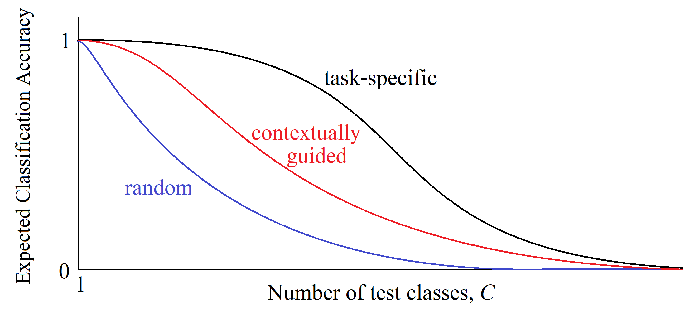
Fig. 2: Transfer Utility of CG-CNN features is based on the area under the curve of the test accuracy $A_{CG}$ as a function of the number of test classes $C$. Accuracies obtained using the random and task-specific CNN features, $A_{random}(C)$ and $A_{specific}(C)$ are also shown as they are used in Eq. 7 to quantify the Transfer Utility, $U$. The expectation of the test accuracies is computed over a number of tasks generated for each value of $C$.

3.4 Sources of Contextual Guidance

While in our presentation of CG-CNN so far we have explained the use of contextual guidance on an example of spatial proximity, using neighboring image patches to define training/testing classes, any other kind of contextual relations can also be used as a source of guidance in developing CNN-layer features. Temporal context is one such rich source. Frequency domain context is another source, most obviously in speech recognition, while in Section 4 we exploit it in a form of hyperspectral imaging. More generally, any natural phenomena in which a core of indigenous causally influential factors are reflected redundantly in multivariable raw sensor data will have contextual regularities, which might be possible to use to guide feature learning in the CNN layer.

With regard to spatial-proximity-based contextual grouping, it is different from data augmentation used in deep learning Dosovitskiy et al., (2014). Data augmentation does shift input image patches a few pixels in each direction to create more examples of a known object category (such as a car or an animal); however, for a contextual group, we do not have such object categories to guide the placement of image patches and we take patches over a much larger range pixels from the center of the contextual group. Training CG-CNN using short shifts (similar to data-augmentation) does not lead to tuning to V1-like features because other/suboptimal features can also easily cluster heavily overlapping image patches.

Another source of contextual information that we utilize in this paper for extracting features from color images is based on multiple pixel-color representations (specifically, RGB and grayscale). Instead of using a feature-engineering approach that learns to extract color features and grayscale features separately, as in Krizhevsky et al., (2012), we use a data-engineering approach by extending the contextual group formation to the color and gray versions of the image windows: For every contextual group, some of the RGB image patches are converted to grayscale. This helps our network develop both gray and color features as needed for maximal transfer utility: if the training is performed only on gray images, even though the neurons might have access to separate RGB color channels, whose weights are randomly initialized and the visualization of feature weights initially looks colorful, they all gradually move towards gray features. Using no grayscale images leads to all-color features automatically. For our experiments in Section 4, the probability for the random grayscale transformation was set to 0.5. That is, we converted 50% of the image patches in each contextual group from color to gray, which led to emergence of gray-level features in addition to color ones.

4 Experimental Results

4.1 Demonstration on Natural Images

To demonstrate the feasibility of CG-CNN developing pluripotent features using a limited number of images without any class-labels, we used images from the Caltech-101 dataset Fei-Fei et al., (2007). We used images from a single (face) class to emphasize that the proposed algorithm does not use any external supervision for tuning to its discriminatory features. Thus, our dataset had 435 color images, with sizes varying around $400\times 600$ pixels (see Fig. 3 for two representative examples). We used half of these images to train CG-CNN and develop its features and the other half to evaluate pluripotency of these features.

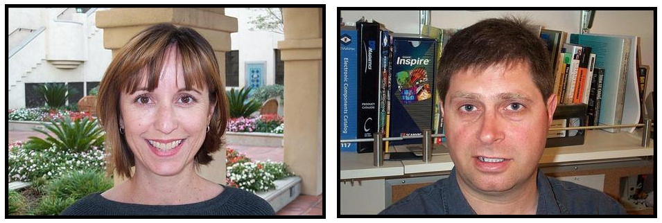
Fig. 3: Two exemplary images from Caltech-101 dataset used for snipping small image patches for the CG-CNN training. Only images that belong to the face-class were used in order to show that CG-CNN can develop its features on a small dataset without relying on class-labels or external supervision.

Since our CG-CNN algorithm can be used with any CNN architecture, we applied it to AlexNet, ResNet, and GoogLeNet architectures. In its first convolutional block, AlexNet performs Conv+ReLU+MaxPool. This first block has $d=64$ features, with a kernel size of $11\times 11$ (i.e., $w=11$) and a stride $s=4$ pixels. ResNet performs Conv+BatchNorm+ReLU+MaxPool in its first block, with $d=64$ features, kernel size of $7\times 7$, and stride $s=2$ pixels. GoogLeNet in its first block also has $d=64$ features, $7\times 7$ kernels, and stride $s=2$. However, GoogLeNet performs Conv+BatchNorm+MaxPool. All three architectures use MaxPool with a kernel size of $3\times 3$ and a stride $s=2$. Therefore, the viewing window of a MaxPool unit is 19 pixels for AlexNet and 11 pixels for ResNet and GoogLeNet. (Note that although we could enrich these architectures by adding drop-out and/or local response normalization to adjust lateral inhibition, we chose not to do such optimizations in order to show that pluripotent features can develop solely under contextual guidance.)

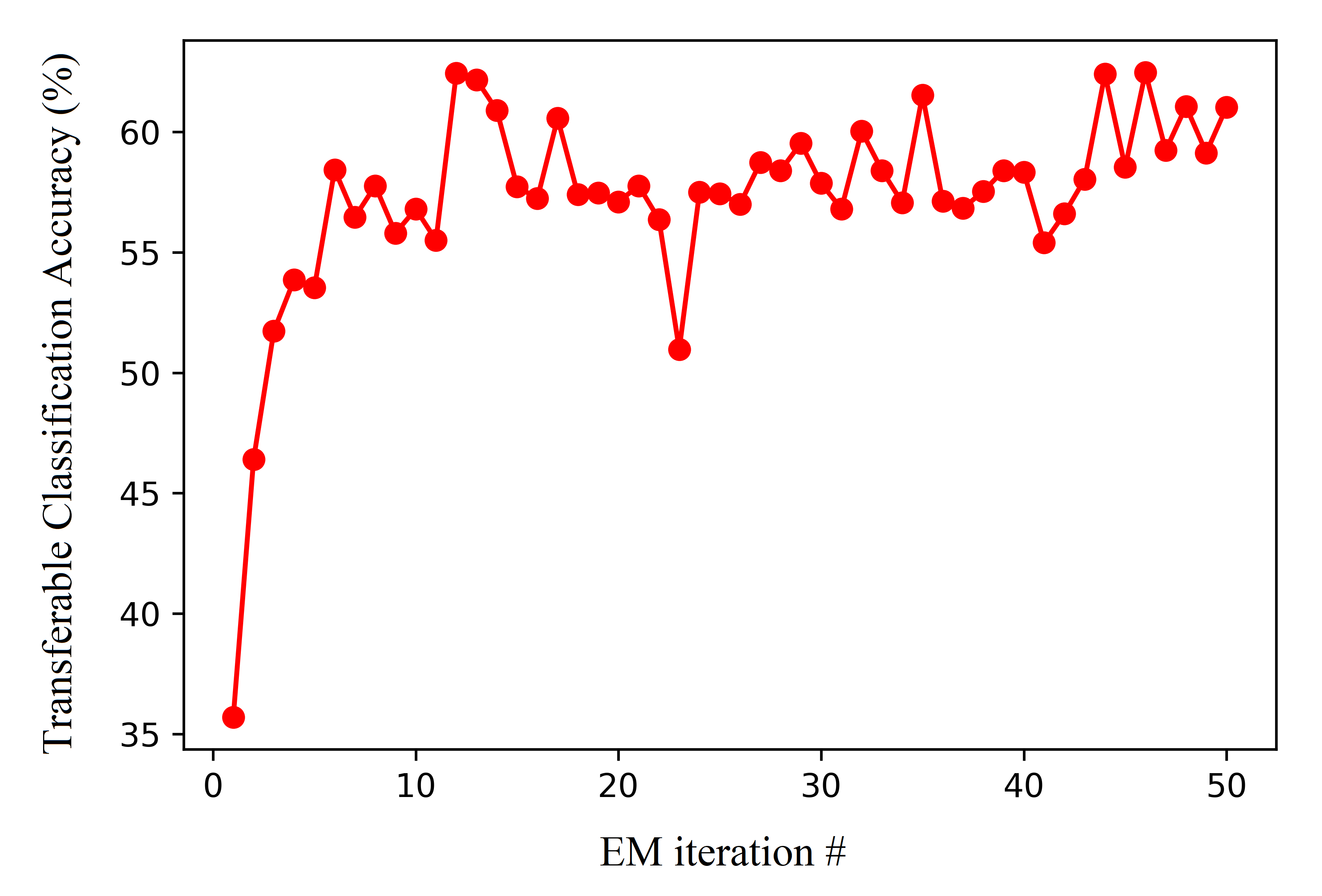
Fig. 4: Transferable Classification Accuracy (Eq. 6) plotted as a function of EM iterations during training of AlexNet-compatible CG-CNN.

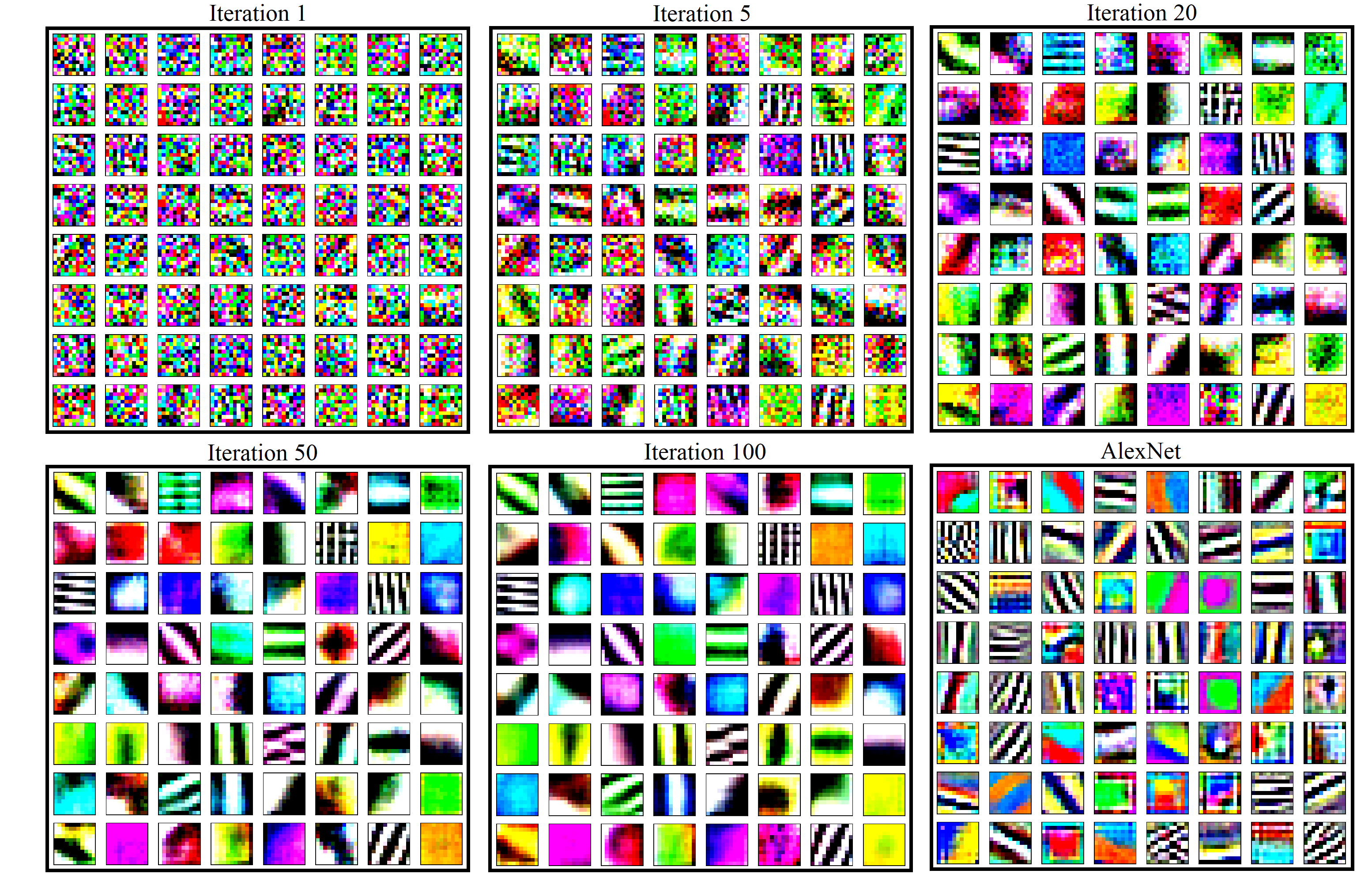
Fig. 5: Visualizations of the $11\times 11$ weights of the 64 features in the CNN layer of CG-CNN after 1, 5, 20, 50, and 100 EM iterations. Also shown are the weights of the 64 features in the first layer of AlexNet. While even after 20 EM iterations the features are still quite crude, the features at iterations 50 and 100 are sharp and almost identical and resemble AlexNet features.

We used a moderate number of contextual groups ($C=100$) for the CG-CNN training. For selecting image patches for each contextual group, the parameter $g$ – used in Algorithm 1 to slide the seed window for spatial contextual guidance – was set to $g=25$ pixels. Thus, each contextual group had $(2\times 25+1)^{2}=2601$ distinct patch positions. We also used color jitter and color-to-gray conversion to enrich contextual groups (see Section 3.4).

We used PyTorch open source machine learning framework Paszke et al., (2019) to implement CG-CNN. Experiments were performed on a workstation with Intel i7-9700K 3.6GHz CPU with 32 GB RAM and NVIDIA GeForce RTX 2080 GPU with 8GB GDDR6 memory. In each EM training iteration, we used 10 epochs for the E-step and 10 epochs for the M-step. On the workstation used for the experiments, for $C=100$, each EM iteration takes about two minutes. CG-CNN takes around 100 minutes to converge in about 50 iterations. Both the SGD (stochastic gradient descent) and Adam Kingma & Ba, (2017) optimizers can reduce time. Adam helps cut down the runtime by reducing the number of epochs down to one epoch with minibatch updates. Increasing the number of EM iterations was more helpful than increasing the number of epochs in one iteration. With these improvements, 50 EM iterations took about 10 minutes.

Figure 4 shows the time-course of the transferable classification accuracy (Eq. 6) improvements during network training, which rises quickly in the first few EM iterations and then slowly converges to a stable level. Most of the improvements are accomplished in the first 50 iterations. With each EM iteration, the network’s features become progressively more defined and more resembling visual cortical features (gratings, Gabor-like features, and color blobs) as well as features extracted in the early layers of deep learning architectures AlexNet, GoogLeNet, and ResNet (see Figs. 5 and 6).

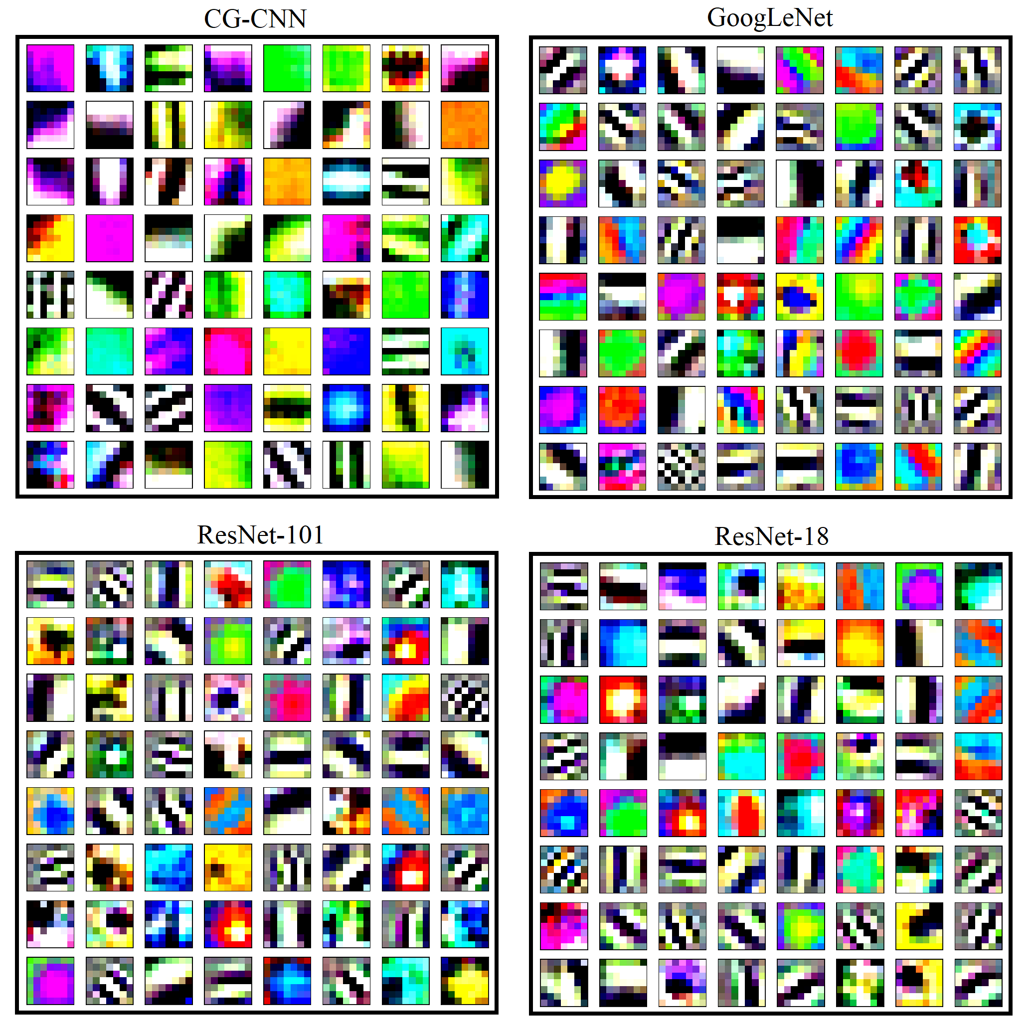
Fig. 6: Visualizations of the $7\times 7$ weights of the 64 features in the CNN layer of CG-CNN after 100 EM iterations, as well as 64 features in the first layer of GoogLeNet, ResNet-101, and ResNet-18.

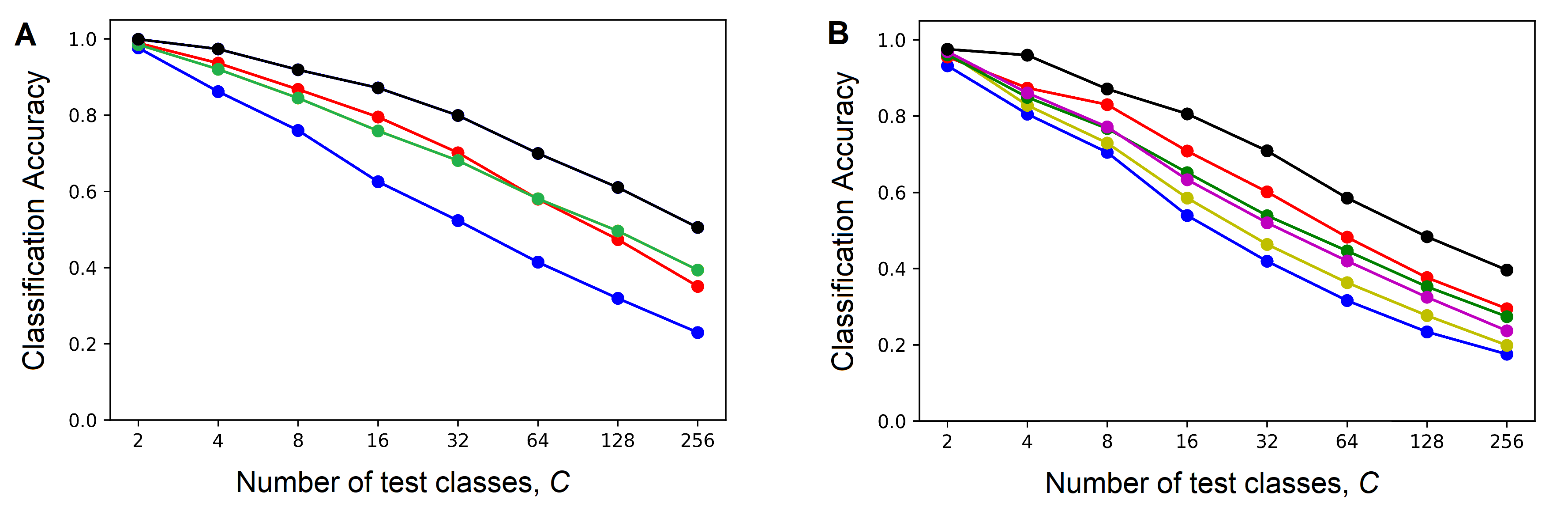
Fig. 7: Transfer Utility of GC-CNN features, demonstrated following the format of Figure 2. (A) $11\times 11$ pixel features. Average Classification Accuracies of CNN-Classifiers with task-specific, random, and CG features ($A_{specific}$, $A_{random}$, and $A_{CG}$; black, blue, and red curves, respectively) are plotted as a function of the number of contextual classes used in a classification task. For a comparison, also plotted is the average Classification Accuracy of CNN-Classifiers with Pool-1 features of the pretrained AlexNet (green curve). (B) $7\times 7$ pixel features. Average Classification Accuracies of CNN-Classifiers with task-specific (black), random (blue), and CG (red) features are plotted as a function of the number of test classes. For a comparison, also plotted are the average Classification Accuracies of CNN-Classifiers with Pool-1 features of the pretrained GoogLeNet (green), ResNet-101 (magenta), and ResNet-18 (yellow) networks.

To compare pluripotency of CG-CNN features to pluripotency of AlexNet, ResNet, and GoogLeNet features, we used the Transfer Utility approach described in Section 3.3 (see Fig. 2 and Eq. 7) and tested classification accuracy of CNN-Classifiers equipped with random, task-specific, and CG features, as well as pretrained AlexNet, GoogLeNet, and ResNet features, on new contextual groups/classes drawn from the test set images that were not used during the training of CG-CNN. These classification accuracy estimates are plotted in Figure 7 as a function of the number of test classes $C$ in each classification task. As the two plots in Figure 7 show, the curves generated with CG-CNN features lay slightly more than halfway between the curves generated with random and task-specific features, indicating substantial degree of transfer utility. Most importantly, CG-CNN curves match or even exceed the curves generated with features taken from deep CNN systems, which are acknowledged – as reviewed in Sections 1 and 2.1 – to have desirable levels of transfer utility.

4.2 Demonstration on Texture Image Classification

As an additional test of pluripotency of CG-CNN features, we applied them to a texture classification task. Texture is a key element of human visual perception and texture classification is a challenging computer vision task, utilized in applications ranging from image analysis (e.g. biomedical and aerial) to industrial automation, remote sensing, face recognition, etc. Anam & Rushdi, (2019). For this test, we used the Brodatz dataset Brodatz, (1966) of 13 texture images, in which each image shows a different natural texture and is $512\times 512$ pixels in size (Fig. 8). To compare with AlexNet (which has $11\times 11$ pixel features, stride $s=4$, and therefore pooled window size of $19\times 19$ pixels), we trained classifiers to discriminate textures in $19\times 19$ pixel Brodatz image patches. To compare with GoogLeNet and ResNet (which have $7\times 7$ pixel features, stride $s=2$, and therefore pooled window size of $11\times 11$ pixels), we trained other classifiers to discriminate textures in $11\times 11$ pixel Brodatz image patches. For either of these two window sizes, we subdivided each $512\times 512$ texture image into 256 $32\times 32$ subregions and picked 128 training image patches at random positions within 128 of these subregions, and other 128 test image patches at random positions within the remaining 128 subregions. This selection process ensured that none of the training and test image patches overlapped to any degree, while sampling all the image territories.

Using the $128\times 13=1664$ training image patches, we trained CNN-Classifiers equipped with either CG-CNN features (previously developed on Caltech-101 images, as described above in Section 4.1), or AlexNet, GoogLeNet, or ResNet features. Note that these features were not updated during classifier training; i.e., they were transferred and used “as is” in this texture classification task. For additional benchmarking comparison, to gauge the difficulty of this texture classification task, we also applied some standard machine learning algorithms Fernandez-Delgado et al., (2014), including Decision Trees and Random Forests, Linear and RBF SVMs, Logistic Regression, Naive Bayes, MLP (Multi-Layer Perceptron), and K-NN (K-Nearest Neighbor).

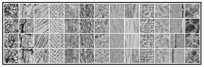
Fig. 8: Brodatz texture images. Shown are 4 representative $50\times 50$ pixel extracts from each of the 13 $512\times 512$ pixel images in the dataset. CG-CNN and 11 other classifiers were trained to identify these textures based on either $11\times 11$ or $19\times 19$ pixel image patches (see main text for details).

These classifiers are straightforward to optimize without requiring many hyperparameters. For their implementation (including optimization/validation of the classifier hyperparameters), we used scikit-learn Python module for machine learning Pedregosa et al., (2011). For MLP, we used a single hidden layer with ReLU activation function (we used 64 hidden units in the layer to keep the complexity similar to that of CG-CNN). We used the default value for the regularization parameter ($C=1$) for our SVMs and the automatic scaling for setting the RBF radius for RBF-SVM. We used $K=1$ neighbor and the Euclidean distance metric for K-NN. For the random forest classifier, we used 100 trees as the number of estimators in the forest.

All the classifiers were tested on the image patches from the test set, not used in classifier training. There are a total of $128\times 13=1664$ test image patches. The accuracies of the classifiers are listed in Table 1. According to this table, all the CNN-classifiers with transferred features had very similar texture classification accuracies, with CG features giving the best performance. All the other classifiers performed much worse, indicating non-trivial nature of this classification task. These results demonstrate the superiority of using the transfer learning approach, with transferred features taken from CG-CNN or Pool-1 of pretrained deep networks.

Table 1: Texture classification accuracies of 12 classifiers on 13 textures taken from the Brodatz (1966) dataset. Listed are means and standard deviations of the means computed over 10 test runs.

Method	$11\times 11$ field	$19\times 19$ field
CG-CNN	63.3 $\pm$ 0.7	74.3 $\pm$ 0.9
AlexNet		72.2 $\pm$ 0.7
GoogLeNet	62.2 $\pm$ 1.1
ResNet-101	61.6 $\pm$ 0.9
ResNet-18	61.5 $\pm$ 0.9
RBF-SVM	53.6 $\pm$ 0.9	62.9 $\pm$ 0.9
Naive Bayes	39.3 $\pm$ 1.0	49.4 $\pm$ 0.8
Random Forest	34.7 $\pm$ 1.3	35.0 $\pm$ 1.5
MLP	33.6 $\pm$ 0.7	30.7 $\pm$ 0.6
K-NN	28.6 $\pm$ 0.9	29.2 $\pm$ 0.8
Linear-SVM	23.3 $\pm$ 1.2	28.0 $\pm$ 1.9
LR	22.8 $\pm$ 1.5	25.1 $\pm$ 0.6

4.3 Demonstration on Hyperspectral Image Classification

Unlike color image processing that uses a large image window with a few color channels (grayscale or RGB), Hyperspectral Image (HSI) analysis typically aims at classification of a single pixel characterized by a high number of spectral channels (bands). Typically, HSI datasets are small, and application of supervised deep learning to such small datasets can result in overlearning, not yielding pluripotent task-transferrable HSI-domain features Sellami et al., (2019). To improve generalization, the supervised classification can benefit from unsupervised feature extraction of a small number of more complex/informative features than the raw data in the spectral channels. In this section, we demonstrate the usefulness of the features extracted by the proposed CG-CNN algorithm on the Indian Pines and Salinas datasets, which are well-known HSI datasets captured by the AVIRIS (Airborne Visible/Infrared Imaging Spectrometer) sensor.

The Indian Pines dataset is a $145\times 145$ pixel image with 220 spectral channels (bands) in the 400-2500 nm range of wavelengths Grana et al., (2018). The dataset includes 16 classes, some of which are various crops and others are grass and woods. Fig. 9A shows the color view and the ground truth of the image. Table 3 lists the class names and the number of examples. The Salinas dataset is a $512\times 217$ HSI image with 220 spectral bands Grana et al., (2018). There are 16 classes in the dataset including vegetables, bare soils, and vineyard fields. Fig. 9B shows the color view and the ground truth of the image and Table 3 lists each class and the number of examples.

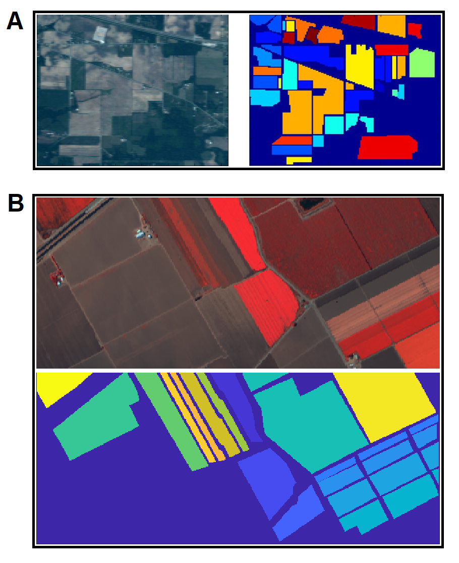
Fig. 9: Hyperspectral Image dataset. (A) The Indian Pines image (left) and its ground truth labeling (right). (B) The Salinas image (top) and its ground truth labeling (bottom).

Table 2: The class names and the number of examples in each class of the Indian Pines dataset

Num	Class	Examples
1	Alfalfa	54
2	Corn-notill	1434
3	Corn-mintill	834
4	Corn	234
5	Grass-pasture	497
6	Grass-trees	747
7	Grass-pasture-mowed	26
8	Hay-windrowed	489
9	Oats	20
10	Soybean-notill	968
11	Soybean-mintill	2468
12	Soybean-clean	614
13	Wheat	212
14	Woods	1294
15	Build.-Grass-Trees-Drv.	380
16	Stone-Steel-Towers	95
Total		10366

Table 3: The class names and the number of examples in each class of the Salinas dataset

Num	Class	Examples
1	Brocoli (green weeds 1)	2009
2	Brocoli (green weeds 2)	3726
3	Fallow	1976
4	Fallow (rough plow)	1394
5	Fallow (smooth)	2678
6	Stubble	3959
7	Celery	3579
8	Grapes (untrained)	11271
9	Soil (vinyard develop)	6203
10	Corn (senesced green weeds)	3278
11	Lettuce (romaine 4wk)	1068
12	Lettuce (romaine 5wk)	1927
13	Lettuce (romaine 6wk)	916
14	Lettuce (romaine 7wk)	1070
15	Vinyard (untrained)	7268
16	Vinyard (vertical trellis)	1807
Total		54129

To evaluate the quality of CG-CNN features on the hyperspectral data, the CG-CNN architecture presented in Algorithm 1 was used with the following parameters: $a=3$ pixels, $b=220$ bands, $d=30$ features, $w=1$ pixel (i.e., each convolution uses only the bands of a single pixel), $C=20$ contextual groups, and $g=2$ pixels for the extent of the spatial contextual guidance. In training of CG-CNN, the class labels of the HSI pixels were not used; instead, local groups of pixels (controlled by the $g$ parameter) were treated as training classes, as described in Section 3.4. CG-CNN learns to represent its input HSI image patch, which is a hypercube of size $3\times 3\times 220$, in such a way that the image patch and its neighboring windows/positions (obtained by shifting it $g=\pm 2$ pixels in each direction) can be maximally discriminable from other contextual groups centered elsewhere. Note that only a total of $(2\times 2+1)^{2}=25$ image patches are created for each contextual group. (We can also enrich contextual groups by adding band-specific noise or frequency shift, but leave this for future work.) Then, we used the extracted features as inputs to various supervised classifiers. Decision Trees (ID3), Random Forests (RF), Linear Discriminant Analysis (LDA), Linear SVM, RBF SVM, SVM with cubic-polynomial kernel (Cubic-SVM), and K-Nearest Neighbor (K-NN) classifiers were selected due to their popularity and robustness Fernandez-Delgado et al., (2014); Alpaydin, (2014). The $d=30$ features, learned in the CNN-layer of CG-CNN, were fed to these classifiers to use them in the final classification task with 16 target classes (various vegetation, buildings, etc.). Pixel classification accuracies were computed using 10-fold cross validation. For comparison, we evaluated the use of all of the original raw variables (i.e., 220 bands) as inputs to the classifiers and we also compared with first 30 principal components of the Principal Component Analysis (PCA) and best 30 Random Forest (RF) features Breiman, (2001); Fernandez-Delgado et al., (2014) extracted using algorithms available in MATLAB Statistics and Machine Learning Toolbox. We performed our experiments using MATLAB Classification Learner toolbox.

Table 4: HSI classification results on the Indian Pines dataset.

	Accuracy (%)
	Orig.(220)	PCA(30)	RF(30)	CG-CNN(30)
ID3	67.8 $\pm$ 1.1	68.2 $\pm$ 1.3	67.0 $\pm$ 1.9	76.5 $\pm$ 1.6
LDA	79.4 $\pm$ 1.0	61.0 $\pm$ 1.4	62.1 $\pm$ 1.7	72.3 $\pm$ 1.5
Linear-SVM	85.2 $\pm$ 1.7	75.1 $\pm$ 1.4	76.0 $\pm$ 1.3	79.5 $\pm$ 0.8
Cubic-SVM	91.9 $\pm$ 0.8	86.0 $\pm$ 1.0	87.0 $\pm$ 1.0	94.7 $\pm$ 0.7
RBF-SVM	87.1 $\pm$ 0.6	81.5 $\pm$ 0.8	80.7 $\pm$ 1.8	90.5 $\pm$ 1.0
K-NN	76.0 $\pm$ 1.1	74.2 $\pm$ 1.2	80.0 $\pm$ 0.9	95.4 $\pm$ 0.5
RF	86.5 $\pm$ 0.9	82.8 $\pm$ 1.1	83.4 $\pm$ 1.3	96.2 $\pm$ 0.6

Table 5: HSI classification results on the Salinas dataset.

	Accuracy (%)
	Orig.(220)	PCA(30)	RF(30)	CG-CNN(30)
ID3	88.3 $\pm$ 0.6	90.2 $\pm$ 0.3	85.9 $\pm$ 0.5	87.3 $\pm$ 0.5
LDA	91.7 $\pm$ 0.3	90.6 $\pm$ 0.4	89.6 $\pm$ 0.5	88.7 $\pm$ 0.6
Linear-SVM	92.9 $\pm$ 0.4	93.2 $\pm$ 0.3	92.2 $\pm$ 0.4	92.8 $\pm$ 0.4
Cubic-SVM	96.1 $\pm$ 1.5	96.2 $\pm$ 1.0	94.8 $\pm$ 1.0	96.8 $\pm$ 0.2
RBF-SVM	95.2 $\pm$ 0.3	96.5 $\pm$ 0.3	94.1 $\pm$ 0.3	95.7 $\pm$ 0.2
K-NN	91.9 $\pm$ 0.5	92.6 $\pm$ 0.4	93.0 $\pm$ 0.3	97.8 $\pm$ 0.3
RF	95.3 $\pm$ 0.3	96.1 $\pm$ 0.2	95.2 $\pm$ 0.3	97.8 $\pm$ 0.3

Use of CG-CNN features yielded the highest classification accuracies. The results on the Indian Pines dataset are reported in Table 4 and on the Salinas dataset in Table 5. As shown in these tables, the best performance was achieved by combining CG-CNN features with Random Forest or K-NN classifiers. For the best feature and classifier combination (CG-CNN features + RF Classifier), individual class accuracies (precision and recall) were compared with the accuracies obtained by using RF classifier on 220 original/raw features or first 30 PCA features. Tables 6 and 7 show these comparisons for the Indian Pines and Salinas datasets, respectively. CG-CNN features yielded better results for an overwhelming majority of classes.

Table 6: Random Forest classification results for individual classes in the Indian Pines dataset. Original 220 features are compared with 30 PCA and 30 CG-CNN features.

		Precision (%)			Recall (%)
Class	#Examples	Orig. (220)	PCA (30)	CG-CNN (30)	Orig. (220)	PCA (30)	CG-CNN (30)
1	46	94.6	93.1	100.0	76.1	58.7	93.5
2	1428	85.3	71.4	96.1	81.1	74.4	95.3
3	830	85.7	78.4	92.2	71.3	64.5	95.7
4	237	74.1	72.1	97.0	68.8	46.8	95.4
5	483	93.7	92.0	99.4	92.3	90.7	97.5
6	730	90.3	91.1	98.9	97.8	96.2	99.3
7	28	95.2	91.7	100	71.4	78.6	100
8	478	95.6	94.6	99.8	99.2	99.2	100
9	20	92.3	92.9	100	60.0	65.0	90.0
10	972	84.4	76.4	95.3	84.4	78.7	97.9
11	2455	82.9	79.6	96.5	91.2	86.3	97.6
12	593	80.0	75.3	97.3	75.4	66.3	91.1
13	205	96.1	94.3	100	96.1	96.6	99.5
14	1265	93.0	91.1	98.5	96.8	97.5	99.0
15	386	78.2	75.5	95.5	63.2	54.1	88.3
16	93	98.8	96.5	97.9	88.2	89.2	100

Table 7: Random Forest classification results for individual classes in the Salinas dataset. Original 220 features are compared with 30 PCA and 30 CG-CNN features.

		Precision (%)			Recall (%)
Class	#Examples	Orig. (220)	PCA (30)	CG-CNN (30)	Orig. (220)	PCA (30)	CG-CNN (30)
1	2009	99.9	100.0	100.0	100.0	98.4	98.4
2	3726	100.0	100.0	100.0	99.9	99.9	100.0
3	1976	98.8	99.7	99.9	99.8	99.7	99.9
4	1394	99.2	99.9	99.9	99.6	99.8	99.7
5	2678	99.4	99.8	99.8	99.2	99.9	99.9
6	3959	99.9	100.0	100.0	100.0	99.9	100.0
7	3579	99.9	99.9	100.0	99.8	100.0	100.0
8	11271	87.4	90.6	95.8	92.6	92.9	96.3
9	6203	99.5	99.8	99.9	99.8	99.9	99.9
10	3278	97.9	99.1	99.5	97.3	98.4	98.9
11	1068	98.4	99.5	99.7	98.7	98.8	99.1
12	1927	99.3	99.9	100.0	99.7	98.9	99.0
13	916	99.0	99.6	99.9	99.2	98.7	98.9
14	1070	98.8	99.7	99.9	97.9	98.1	98.8
15	7268	87.7	86.4	92.0	79.5	85.1	93.5
16	1807	99.8	99.9	100.0	99.3	95.8	95.9

5 Conclusions

Deep neural networks trained on millions of images from thousands of classes yield inferentially powerful features in their layers. Similar sets of features emerge in many different deep learning architectures, especially in their early layers. These pluripotent features can be transferred to other image recognition tasks to achieve better generalization. The proposed Contextually Guided Convolutional Neural Network (CG-CNN) method is an alternative approach for learning such pluripotent features. Instead of a big and deep network, we use a shallow CNN network with a small number of output units, trained to recognize contextually related input patterns. Once the network is trained on one task, involving one set of different contexts, the convolutional features it develops are transferred to a new task, involving a new set of different contexts, and training continues. In a course of repeatedly transferred training on a sequence of such tasks, convolutional features progressively develop greater pluripotency, which we quantify as a transfer utility (the degree of usefulness when transferred to new tasks). Thus, our approach to developing high utility features combines transfer learning and contextual guidance. In our comparative studies, such CG-CNN features showed the same, if not higher, transfer utility and texture classification accuracy as comparable features in the well-known deep networks – AlexNet, ResNet, and GoogLeNet.

With regard to learning powerful broad-purpose features, CG-CNN has an important practical advantage over deep CNNs in its greatly reduced architectural complexity and size and in its ability to find pluripotent features even in small unlabeled datasets. We demonstrate these advantages by using CG-CNN to find pluripotent features in two small hyperspectral image datasets and showing that with these features we can achieve the best classification performance on these datasets.

Turning to limitations of the CG-CNN design presented in this paper, a single CNN layer is, obviously, limited in the complexity of features it can develop. A series of CNN layers – each developed in its own turn using local contextual guidance on the outputs of the already developed preceding layer(s) – might be expected to extract more globally descriptive features capable of object/target recognition. However, it remains to be determined whether such features will rival pluripotency of features extracted by comparable series of layers in conventional deep CNN. Also it remains to be explored how much contextual information, which might be used in guiding the development of higher-level CNN layers, is present at higher levels. This brings us to an even more fundamental question: How can we recognize and exploit potential sources and kinds of contextual information present in a particular data source? This is a critical question, since it determines how contextual groups (i.e., training classes) will be chosen for EM training of the system. Finally, feedback guidance (FG) from higher to lower CNN layers, combined with local within-layer contextual guidance, would undoubtedly further enhance pluripotency of features developed in such multilayer CG-FG-CNN designs.

Thus, for future work, the proposed CG-CNN architecture can be improved by stacking multiple CG-CNN layers and incorporating other forms of contextual guidance (such as spatiotemporal proximity, feature-based similarity) and feedback guidance from higher CG-CNN layers.

References

- Ahmed et al., (2008) Ahmed, A., Yu, K., Xu, W., Gong, Y., & Xing, E. (2008). Training hierarchical feed-forward visual recognition models using transfer learning from pseudo-tasks. In Forsyth, D., Torr, P., & Zisserman, A., editors, Computer Vision – ECCV 2008, pages 69–82, Berlin, Heidelberg. Springer Berlin Heidelberg.
- Alpaydin, (2014) Alpaydin, E. (2014). Introduction to machine learning, third edition. The MIT Press, Cambridge.
- Anam & Rushdi, (2019) Anam, A. M. & Rushdi, M. A. (2019). Classification of scaled texture patterns with transfer learning. Expert Systems with Applications, 120:448 – 460.
- Arjovsky & Bottou, (2017) Arjovsky, M. & Bottou, L. (2017). Towards principled methods for training generative adversarial networks. In International Conference on Neural Information Processing Systems (NIPS) 2016 Workshop on Adversarial Training. In review for ICLR, volume 2016.
- Becker & Hinton, (1992) Becker, S. & Hinton, G. E. (1992). Self-organizing neural network that discovers surfaces in random-dot stereograms. Nature, 355(6356):161.
- Bengio, (2012) Bengio, Y. (2012). Deep learning of representations for unsupervised and transfer learning. In Proceedings of ICML Workshop on Unsupervised and Transfer Learning, pages 17–36.
- Breiman, (2001) Breiman, L. (2001). Random forests. Machine learning, 45(1):5–32.
- Brodatz, (1966) Brodatz, P. (1966). Textures: A photographic album for artists and designers. Dover Pubns.
- Caruana, (1995) Caruana, R. (1995). Learning many related tasks at the same time with backpropagation. In Advances in Neural Information Processing Systems, pages 657–664.
- Clark & Thornton, (1997) Clark, A. & Thornton, C. (1997). Trading spaces: Computation, representation, and the limits of uninformed learning. Behavioral and Brain Sciences, 20(1):57–66.
- Do & Batzoglou, (2008) Do, C. B. & Batzoglou, S. (2008). What is the expectation maximization algorithm? Nature Biotechnology, 26(8):897–899.
- Dosovitskiy et al., (2014) Dosovitskiy, A., Springenberg, J. T., Riedmiller, M., & Brox, T. (2014). Discriminative unsupervised feature learning with convolutional neural networks. In Advances in Neural Information Processing Systems, pages 766–774.
- Favorov & Kursun, (2011) Favorov, O. V. & Kursun, O. (2011). Neocortical layer 4 as a pluripotent function linearizer. Journal of Neurophysiology, 105(3):1342–1360.
- Favorov & Ryder, (2004) Favorov, O. V. & Ryder, D. (2004). Sinbad: A neocortical mechanism for discovering environmental variables and regularities hidden in sensory input. Biological Cybernetics, 90(3):191–202.
- Fei-Fei et al., (2007) Fei-Fei, L., Fergus, R., & Perona, P. (2007). Learning generative visual models from few training examples: An incremental bayesian approach tested on 101 object categories. Computer Vision and Image Understanding, 106(1):59–70.
- Fernandez-Delgado et al., (2014) Fernandez-Delgado, M., Cernadas, E., Barro, S., & Amorim, D. (2014). Do we need hundreds of classifiers to solve real world classification problems? Journal of Machine Learning Research, 15:3133–3181.
- Finn et al., (2017) Finn, C., Abbeel, P., & Levine, S. (2017). Model-agnostic meta-learning for fast adaptation of deep networks.
- Gao et al., (2020) Gao, F., Yoon, H., Wu, T., & Chu, X. (2020). A feature transfer enabled multi-task deep learning model on medical imaging. Expert Systems with Applications, 143:112957.
- Ghaderi & Athitsos, (2016) Ghaderi, A. & Athitsos, V. (2016). Selective unsupervised feature learning with convolutional neural network (s-cnn). 2016 23rd International Conference on Pattern Recognition (ICPR).
- Glorot & Bengio, (2010) Glorot, X. & Bengio, Y. (2010). Understanding the difficulty of training deep feedforward neural networks. In Teh, Y. W. & Titterington, M., editors, Proceedings of the Thirteenth International Conference on Artificial Intelligence and Statistics, volume 9 of Proceedings of Machine Learning Research, pages 249–256, Chia Laguna Resort, Sardinia, Italy. JMLR Workshop and Conference Proceedings.
- Goodfellow et al., (2016) Goodfellow, I., Bengio, Y., & Courville, A. (2016). Deep learning. MIT Press, Cambridge.
- Grana et al., (2018) Grana, M., Veganzons, M., & Ayerdi, B. (2018). Hyperspectral remote sensing scenes - grupo de inteligencia computacional (GIC). http://www.ehu.eus/ccwintco/index.php. (Accessed on 12/22/2018).
- Grandvalet & Bengio, (2004) Grandvalet, Y. & Bengio, Y. (2004). Semi-supervised learning by entropy minimization. In Proceedings of the 17th International Conference on Neural Information Processing Systems, NIPS’04, page 529–536, Cambridge, MA, USA. MIT Press.
- Grill-Spector & Malach, (2004) Grill-Spector, K. & Malach, R. (2004). The human visual cortex. Annual Review of Neuroscience, 27:649–677.
- Hawkins et al., (2017) Hawkins, J., Ahmad, S., & Cui, Y. (2017). A theory of how columns in the neocortex enable learning the structure of the world. Frontiers in Neural Circuits, 11:81.
- Hawkins & Blakeslee, (2004) Hawkins, J. & Blakeslee, S. (2004). On Intelligence. Times Books, USA.
- Hjelm et al., (2019) Hjelm, R. D., Fedorov, A., Lavoie-Marchildon, S., Grewal, K., Bachman, P., Trischler, A., & Bengio, Y. (2019). Learning deep representations by mutual information estimation and maximization.
- Huang et al., (2006) Huang, G.-B., Zhu, Q.-Y., & Siew, C.-K. (2006). Extreme learning machine: Theory and applications. Neurocomputing, 70(1):489 – 501. Neural Networks.
- Kay & Phillips, (2011) Kay, J. W. & Phillips, W. (2011). Coherent infomax as a computational goal for neural systems. Bulletin of Mathematical Biology, 73(2):344–372.
- Kingma & Ba, (2017) Kingma, D. P. & Ba, J. (2017). Adam: A method for stochastic optimization.
- Krizhevsky et al., (2012) Krizhevsky, A., Sutskever, I., & Hinton, G. E. (2012). Imagenet classification with deep convolutional neural networks. In Advances in Neural Information Processing Systems, pages 1097–1105.
- Kursun & Favorov, (2019) Kursun, O. & Favorov, O. V. (2019). Suitability of features of deep convolutional neural networks for modeling somatosensory information processing. In Pattern Recognition and Tracking XXX, volume 10995, pages 94 – 105. International Society for Optics and Photonics, SPIE.
- Körding & König, (2000) Körding, K. P. & König, P. (2000). Learning with two sites of synaptic integration. Network: Computation in Neural Systems, 11(1):25–39.
- LeCun et al., (2015) LeCun, Y., Bengio, Y., & Hinton, G. (2015). Deep learning. Nature, 521(7553):436.
- Marblestone et al., (2016) Marblestone, A. H., Wayne, G., & Kording, K. P. (2016). Toward an integration of deep learning and neuroscience. Frontiers in Computational Neuroscience, 10:94.
- Pan et al., (2010) Pan, S. J., Yang, Q., et al. (2010). A survey on transfer learning. IEEE Transactions on Knowledge and Data Engineering, 22(10):1345–1359.
- Paszke et al., (2019) Paszke, A., Gross, S., Massa, F., Lerer, A., Bradbury, J., Chanan, G., Killeen, T., Lin, Z., Gimelshein, N., Antiga, L., Desmaison, A., Kopf, A., Yang, E., DeVito, Z., Raison, M., Tejani, A., Chilamkurthy, S., Steiner, B., Fang, L., Bai, J., & Chintala, S. (2019). Pytorch: An imperative style, high-performance deep learning library. In Advances in Neural Information Processing Systems 32, pages 8024–8035. Curran Associates, Inc. [Online documentation for the transforms package is available at: https://pytorch.org/docs/stable/torchvision/transforms.html].
- Pedregosa et al., (2011) Pedregosa, F., Varoquaux, G., Gramfort, A., Michel, V., Thirion, B., Grisel, O., Blondel, M., Prettenhofer, P., Weiss, R., Dubourg, V., Vanderplas, J., Passos, A., Cournapeau, D., Brucher, M., Perrot, M., & Duchesnay, E. (2011). Scikit-learn: Machine learning in python. Journal of Machine Learning Research, 12:2825–2830.
- Phillips et al., (1995) Phillips, W., Kay, J., & Smyth, D. (1995). The discovery of structure by multi-stream networks of local processors with contextual guidance. Network: Computation in Neural Systems, 6(2):225–246.
- Phillips & Singer, (1997) Phillips, W. A. & Singer, W. (1997). In search of common foundations for cortical computation. Behavioral and Brain Sciences, 20(4):657–683.
- Poggio, (2016) Poggio, T. (2016). Deep learning: Mathematics and neuroscience. A Sponsored Supplement to Science, Brain-Inspired intelligent robotics: The intersection of robotics and neuroscience, pp. 9-12.
- Ravi et al., (2017) Ravi, D., Wong, C., Deligianni, F., Berthelot, M., Andreu-Perez, J., Lo, B., & Yang, G.-Z. (2017). Deep learning for health informatics. IEEE Journal of Biomedical and Health Informatics, 21(1):4–21.
- Sellami et al., (2019) Sellami, A., Farah, M., Riadh Farah, I., & Solaiman, B. (2019). Hyperspectral imagery classification based on semi-supervised 3-d deep neural network and adaptive band selection. Expert Systems with Applications, 129:246 – 259.
- Shorten & Khoshgoftaar, (2019) Shorten, C. & Khoshgoftaar, T. (2019). A survey on image data augmentation for deep learning. Journal of Big Data, 6:1–48.
- Simard et al., (1992) Simard, P., Victorri, B., LeCun, Y., & Denker, J. (1992). Tangent prop - a formalism for specifying selected invariances in an adaptive network. In Moody, J., Hanson, S., & Lippmann, R. P., editors, Advances in Neural Information Processing Systems, volume 4. Morgan-Kaufmann.
- Thrun & Pratt, (2012) Thrun, S. & Pratt, L. (2012). Learning to learn. Springer Science & Business Media.
- Yosinski et al., (2014) Yosinski, J., Clune, J., Bengio, Y., & Lipson, H. (2014). How transferable are features in deep neural networks? In Advances in Neural Information Processing Systems, pages 3320–3328.
- Zhao et al., (2019) Zhao, Z., Zheng, P., Xu, S., & Wu, X. (2019). Object detection with deep learning: A review. IEEE Transactions on Neural Networks and Learning Systems, pages 1–21.