Low-redshift compact star-forming galaxies as analogues of high-redshift star-forming galaxies

We compare the relations among various integrated characteristics of $\sim$ 25,000 low-redshift ($z$ $\la$ 1.0) compact star-forming galaxies (CSFGs) from Data Release 16 (DR16) of the Sloan Digital Sky Survey (SDSS) and of high-redshift ($z$ $\ga$ 1.5) star-forming galaxies (SFGs) with respect to oxygen abundances, stellar masses $M_{\star}$, far-UV absolute magnitudes $M_{\rm FUV}$, star-formation rates SFR and specific star-formation rates sSFR, Lyman-continuum photon production efficiencies ($\xi_{\rm ion}$), UV continuum slopes $\beta$, [O iii] $\lambda$5007/[O ii] $\lambda$3727 and [Ne iii] $\lambda$3868/[O ii] $\lambda$3727 ratios, and emission-line equivalent widths EW([O ii] $\lambda$3727), EW([O iii] $\lambda$5007), and EW(H$\alpha$). We find that the relations for low-$z$ CSFGs with high equivalent widths of the H$\beta$ emission line, EW(H$\beta$) $\geq$ 100Å, and high-$z$ SFGs are very similar, implying close physical properties in these two categories of galaxies. Thus, CSFGs are likely excellent proxies for the SFGs in the high-$z$ Universe. They also extend to galaxies with lower stellar masses, down to $\sim$ 10⁶ M_⊙, and to absolute FUV magnitudes as faint as $-$14 mag. Thanks to their proximity, CSFGs can be studied in much greater detail than distant SFGs. Therefore, the relations between the integrated characteristics of the large sample of CSFGs studied here can prove very useful for our understanding of high-$z$ dwarf galaxies in future observations with large ground-based and space telescopes.

1 Introduction

Considerable progress has been made over the past decade in extending our understanding of the physical properties of high-redshift star-forming galaxies (SFGs) and their evolution in the redshift range extending from $z$ $>$ 2 to $z$ $\sim$ 8 – 11 (e.g. Oesch et al. 2016; Wilkins et al. 2016; Salmon et al. 2018; Ishigaki et al. 2018; Strait et al. 2020a, b; Lam et al. 2019b; De Barros et al. 2019; Bouwens et al. 2019). Large samples of galaxies at $z$ $>$ 2 have become available thanks to the release of extensive spectroscopic surveys (e.g. Steidel et al. 2014; Kriek et al. 2015; McLure et al. 2018; Barro et al. 2019).

The deep spectra of high-$z$ galaxies have revealed that their properties are different from those of typical $z$ $\sim$ 0 SFGs. In the Baldwin-Phillips-Terlevich (BPT) diagram (Baldwin et al. 1981), these galaxies are offset to higher [O iii] $\lambda$5007/H$\beta$ ratios at a fixed [N ii] $\lambda$6584/H$\alpha$ ratio (Steidel et al. 2014; Shapley et al. 2015; Sanders et al. 2020a; Topping et al. 2020a, b), as compared to $z$ $\sim$ 0 main-sequence galaxies (Kewley et al. 2013). Strom et al. (2017), Sanders et al. (2020a), and Topping et al. (2020a) attributed this difference to the harder ionising spectrum at a fixed nebular metallicity in high-$z$ SFGs, whereas Kewley et al. (2013) and Steidel et al. (2014) suggested that in addition to a harder ionising radiation, a higher ionisation parameter and a higher number density or a higher N/O abundance ratio can also shift the relation for high-$z$ SFGs to higher [O iii] $\lambda$5007/H$\beta$ and [N ii] $\lambda$6584/H$\alpha$ ratios.

A common feature of high-$z$ SFGs is the presence of hydrogen Ly$\alpha$, H$\beta,$ and H$\alpha$ emission lines, as well as the presence of some forbidden emission lines – most often of the [O ii] $\lambda$3727, [O iii] $\lambda$4959, 5007, [N ii] $\lambda$6584 emission lines (in the rest-frame optical spectra), or C iii] $\lambda$1906, 1909 emission lines (in the rest-frame UV spectra). This allows us to derive oxygen abundances 12 + log O/H, most commonly with the use of the strong-line calibrations (e.g. Pettini & Pagel 2004), which link strong-line fluxes and 12 + log O/H. The results of these determinations have been presented by Cullen et al. (2014), Troncoso et al. (2014), Onodera et al. (2016), Sanders et al. (2015), Vanzella et al. (2020), Sanders et al. (2020b), and others. In the rarer cases when the weak [O iii] $\lambda$4363 emission-line is detected (Amorín et al. 2016; Kojima et al. 2017, 2020), the direct $T_{\rm e}$ method may be used. Various studies have established that $z$ $\geq$ 2 mass-metallicity relations (MZR) based on oxygen are offset by $\sim$ 0.3 – 0.7 dex to lower metallicities relative to typical main-sequence SFGs at $z$ $\sim$ 0.

Mannucci et al. (2010) introduced an additional parameter, namely, the star formation rate (SFR), which is higher in SFGs at larger $z$. They proposed the use of a more general relation, that is, the fundamental mass-metallicity relation (FMR) and replacing $M_{\star}$ with SFR^-α$M_{\star}$. Mannucci et al. (2010) found that the (12+logO/H) – SFR^-α$M_{\star}$ relation is unique for SFGs at any redshift if $\alpha$ = 0.32. On the other hand, Curti et al. (2020) derived $\alpha$ = 0.55.

The $M_{\star}$ – SFR and $M_{\star}$ – specific SFR (defined as sSFR = SFR/$M_{\star}$) relations are most commonly derived for high-$z$ SFGs (e.g. Whitaker et al. 2014; Salmon et al. 2015; Shivaei et al. 2015; Onodera et al. 2016; Mármol-Queraltó et al. 2016; Smit et al. 2016; Karman et al. 2017; Santini et al. 2017; Iyer et al. 2018; Davidzon et al. 2018; Khusanova et al. 2020). Stellar masses are usually obtained from the spectral energy distribution (SED) in the rest-frame UV range, which is derived adopting a certain star formation history (SFH). The SFR and sSFR are derived either from the UV luminosity, from the UV SED, or from the luminosities of hydrogen emission lines (Ly$\alpha$, H$\beta$, H$\alpha$). Some of these above-cited works found that the slope of the $M_{\star}$ SFR relation is steeper at low stellar masses and that the SFR increases with $z$ at a fixed $M_{\star}$ (e.g. Whitaker et al. 2014). However, Iyer et al. (2018) found that log SFR – log $M_{\star}$ at $z$ = 6 remains linear down to log ($M_{\star}$/M_⊙) = 6. Similarly, the average sSFR systematically increases with increasing $z$ (Mármol-Queraltó et al. 2016; Davidzon et al. 2018), whereas Salmon et al. (2015) found an unevolving correlation between stellar mass and SFR between $z$ = 6 and $z$ = 4. Furthermore, for instance, Santini et al. (2017) have shown that the increase in the sSFR with redshift is milder than predicted by theoretical models and that the sSFR is nearly constant at $z$ $>$ 2 with an average value of $\sim$ 3 Gyr^-1. For comparison, Strom et al. (2017) found sSFR $\sim$ 3 – 40 Gyr^-1 in the redshift range of $z$ $\sim$ 2 – 3.

It was found that high-$z$ SFGs have small sizes in both the FUV continuum and Ly$\alpha$ emission line (e.g. Hagen et al. 2016; Bouwens et al. 2017; Paulino-Afonso et al. 2017, 2018; Matthee et al. 2018; Marchi et al. 2019). In particular, Hagen et al. (2016) and Paulino-Afonso et al. (2017) noted that the brightness distribution in $z$ $\sim$ 2 SFGs are characterised by exponential scales $r_{\rm e}$ = 0.5 – 3.0 kpc. Bouwens et al. (2017) found extremely small sizes of faint $z$ $\sim$ 2 – 8 galaxies with half-light radii $\sim$ 100 – 200 pc for $M_{\rm FUV}$ $\sim$ –15 mag, whereas Matthee et al. (2018) derived $r_{50,{\rm Ly}\alpha}$ $\sim$ 0.3 kpc for the luminous ($M_{\rm FUV}$ = –21.6) SFG COLA1 at $z$ = 6.593. It was also found that galaxies with brighter Ly$\alpha$ emission lines tend to be more compact both in the UV and in Ly$\alpha$ (Paulino-Afonso et al. 2018; Marchi et al. 2019). For comparison, the confirmed low-$z$ LyC leakers and CSFGs with extremely high O₃₂ = [O iii]$\lambda$5007/[O ii]$\lambda$3727 ratios of $>$ 20 show, in the HST NUV images, a compact morphology with $r_{\rm e}$ $\sim$ 0.1 – 1.4 kpc (Izotov et al. 2016a, b, 2018a, 2018b, 2020).

The slope $\beta$ determined from the relation $F_{\lambda}$ $\propto$ $\lambda^{\beta}$ of the UV spectra in high-$z$ SFGs is steep. Bouwens et al. (2012, 2014) and Yamanaka & Yamada (2019) found that $\beta$ in SFGs at $z$ $\sim$ 4 – 8 is in the range of –1.5 - –2.4, whereas Wilkins et al. (2016) derived $\beta$ $\sim$ –1.9 - –2.3 for $z$ $\sim$ 10 galaxies, with the UV slope becoming steeper for the higher redshift SFGs. Additionally, Bouwens et al. (2012, 2014) found a steeper $\beta$ for SFGs with lower $M_{\star}$ and fainter UV luminosities. Pentericci et al. (2018) derived a similar range of $\beta$ for $z$ $\sim$ 6. Santos et al. (2020) determined steep $\beta$ $\sim$ –2.0 and $M_{\star}$ $\sim$ 2$\times$10⁹ M_⊙ for $\sim$ 4000 Lyman-alpha emitters (LAEs) at $z$ = 2 – 6. They concluded that typical star-forming galaxies at high redshift effectively become LAEs.

The steep slopes in the UV range and the strong emission lines of high-$z$ SFGs indicate the presence of massive stellar populations which produce copious amounts of ionising photons. It has thus been suggested that SFGs are the main source of the reionisation of the Universe given that the product $\xi_{\rm ion}$$\times$$f_{\rm esc}$(LyC) is sufficiently high, where $\xi_{\rm ion}$ is the Lyman-continuum production efficiency and $f_{\rm esc}$(LyC) is the fraction of the LyC radiation escaping galaxies. Currently, direct observations of the LyC have resulted in the discovery of approximately three dozens of LyC leakers at high redshifts, with reliably high LyC escape fractions (Vanzella et al. 2015; De Barros et al. 2016; Shapley et al. 2016; Bian et al. 2017; Vanzella et al. 2018; Rivera-Thorsen et al. 2019; Steidel et al. 2018; Fletcher et al. 2019). The parameter $\xi_{\rm ion}$ is derived from synthesis models and it depends on metallicity, star formation history, age, and assumptions on stellar evolution. Values of log [$\xi_{\rm ion}$/Hz erg^-1] $\sim$ 25.2 – 25.3 are typically assumed in studies of the reionisation of the Universe.

Several analyses have indicated that $\xi_{\rm ion}$ in high-$z$ SFGs is similar to or above the canonical value. Bouwens et al. (2015, 2016) found log [$\xi_{\rm ion}$/Hz erg^-1] $\sim$ 25.3 for $z$ = 4 – 5 galaxies and 25.5-25.8 for galaxies with the largest $\beta$. Nakajima et al. (2018, 2020) and Faisst et al. (2019) found an increase of $\xi_{\rm ion}$ for fainter objects at $z$ $\sim$ 3 – 6. Finkelstein et al. (2019) explored scenarios for reionising the intergalactic medium with low galactic ionising photon escape fractions. They found that the ionising emissivity from the faintest galaxies ($M_{\rm FUV}$ $>$ –15 mag) is expected to be dominant. The ionising emissivity from this model is consistent with observations at $z$ = 4 – 5.

An extreme [O iii] $\lambda$5007 line emission associated with a high O₃₂ ratio are common features of the early-lifetime phase for SFGs at $z$ $>$ 2.5 (Cohn et al. 2018; Holden et al. 2016; Tang et al. 2019; Reddy et al. 2018). A high fraction of SFGs at $z$ $>$ 2 with extreme O₃₂ are LAEs (Erb et al. 2016). It was found that [O iii]5007/H$\beta$ emission-line ratios increase with redshift out to $z$ $\sim$ 6 (Cullen et al. 2016; Faisst et al. 2016), attaining values similar to the ratios in local SFGs with high EW(H$\alpha$). This increase results in high EW([O iii] 5007) $>$ 1000$\AA$ for bright $z$ $>$ 7 galaxies (Roberts-Borsani et al. 2016).

The properties of the high-$z$ SFGs discussed above contrast with those of the $z$ $\sim$ 0 main-sequence SFGs. The latter exhibit, on average, a much lower level of star formation activity and, thus, they are characterised by much lower SFRs, sSFRs, and EWs of emission lines at a fixed stellar mass. However, there is a small fraction of low-$z$ SFGs with compact structure and other properties that are similar to those of high-$z$ galaxies. Subsets of these compact star-forming galaxies (CSFGs) are variously called blue compact dwarf (BCD) galaxies, ‘green pea’ (GP) galaxies, and luminous compact galaxies (LCGs) in the literature.

BCDs are nearby dwarf galaxies at redshift $z$ typically $\leq$ 0.01 – 0.02, with strong bursts of star formation and low oxygen abundances of 12 + logO/H $\la$ 7.9, extending down to 12 + logO/H $\la$ 7.0 (e.g. Thuan & Martin 1981; Izotov et al. 1994, 2018c). Typically, their stellar masses are low, $M_{\star}$ $\la$ 10⁸M_⊙. A subset of the lowest-mass BCDs with $M_{\star}$ $\sim$ 10⁶ – 10⁷ M_⊙ and very high O₃₂ $\ga$ 10 has been named ‘blueberry’ galaxies by Yang et al. (2017) because of their compact structure and intense blue colour on the SDSS composite images.

Cardamone et al. (2009) considered ‘green pea’ (GP) galaxies in the redshift range of $z$ = 0.112 – 0.360, with unusually strong [O iii]$\lambda$5007 emission lines, similar to high-$z$ UV-luminous galaxies, such as Lyman-break galaxies and LAEs, with sSFRs up to $\sim$ 10 Gyr^-1. The green colour of these galaxies on composite SDSS images is due to strong [O iii]$\lambda$5007 line emission (with EWs up to 1000$\AA$), redshifted into the SDSS $r$-band.

Izotov et al. (2011) studied a much larger sample of 803 star-forming luminous compact galaxies (LCGs) in a larger redshift range $z$ = 0.02 – 0.63, with global properties similar to those of the GPs. The sSFRs in LCGs are extremely high and vary in the range $\sim$ 1 – 100 Gyr^-1, comparable to those derived in high-$z$ SFGs. Similar high sSFRs were also found for low-$z$ LyC leaking galaxies (Izotov et al. 2016a, b, 2018a, 2018b; Schaerer et al. 2016) and some other low-$z$ SFGs (e.g. Senchyna et al. 2017; Yuma et al. 2019). Izotov et al. (2016c) found sSFRs of up to 1000 Gyr^-1 in a sample of $\sim$ 13000 CSFGs selected from the SDSS. Compared to BCDs, both GPs and LCGs are characterised by higher stellar masses $\sim$ 10⁹ M_⊙ and higher oxygen abundances $\sim$ 7.8 – 8.3.

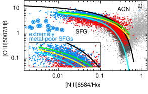
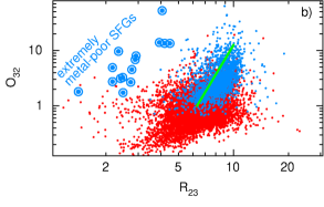
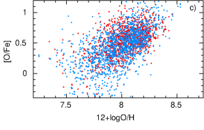
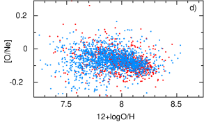
Figure 1: (a) [O iii] $\lambda$5007/H$\beta$ vs. [N ii] $\lambda$6584/H$\alpha$ BPT diagram (Baldwin et al. 1981) for SDSS DR16 CSFGs with EW(H$\beta$) $\geq$ 100$\AA$ (blue dots) and with EW(H$\beta$) $<$ 100$\AA$ (red dots). The SDSS DR7 galaxies including both SFGs (without constraints used for selection of CSFGs) and AGN are represented by dark grey dots and light grey dots, respectively. The black line (Kauffmann et al. 2003) separates SFGs from AGN, whereas the cyan line by Kewley et al. (2013) represents the best fit relation for the total sample of $z$ $\sim$ 0 SFGs from the SDSS DR7. Yellow and green lines indicate relations for $z$ $\sim$ 2 – 3 SFGs by Shapley et al. (2015) and Strom et al. (2017), respectively. An expanded version of the upper part of the diagram in the ranges [N ii]$\lambda$6584/H$\alpha$ of 0.006 - 0.16 and [O iii] $\lambda$5007/H$\beta$ of 4 - 8 is shown in the inset. (b) Relation O₃₂ – R₂₃, where O₃₂ = [O iii] $\lambda$5007/[O ii] $\lambda$3727, R₂₃ = ([O iii] $\lambda$4959 + [O iii] $\lambda$5007 + [O ii] $\lambda$3727)/H$\beta$. The green line represents the relation for $z$ $\sim$ 2 – 3 SFGs by Strom et al. (2017). The most metal-poor nearby galaxies with 12 + log O/H $\sim$ 6.9 – 7.25 (Izotov et al. 2018c; Kojima et al. 2020, Izotov et al., in preparation) are shown in (a) and (b) by encircled blue-filled circles. (c) Dependence of the oxygen overabundance [O/Fe] $\equiv$ log(O/Fe) – log(O/Fe)_⊙ on the oxygen abundance 12 + logO/H. (d) Dependence of [O/Ne] $\equiv$ log(O/Ne) – log(O/Ne)_⊙ on the oxygen abundance 12 + logO/H. Abundances are derived using the $T_{\rm e}$ method. About $\sim$ 2300 galaxies with detected [O iii]$\lambda$4363 emission and an error less than 25% of the line flux are shown in (c) and (d). The meanings of the symbols for SDSS galaxies in (b) – (d) are the same as in (a).

Izotov et al. (2015) selected $\sim$ 5200 low-redshift (0 $<$ $z$ $<$ 1) CSFGs and studied the relations between the global characteristics of this sample, including absolute optical magnitudes, SFRs, stellar masses, and oxygen abundances. They found that for all relations, low-$z$ and high-$z$ SFGs are closely related, indicating a very weak dependence of metallicity on stellar mass, redshift, and star formation rate. This finding favours the assumption of a universal character for the global relations with regard to CSFGs with high-excitation H ii regions over the redshift range 0 $<$ $z$ $<$ 3.

Furthermore, Izotov et al. (2016b, 2018a, 2018b, 2020), in studying high-resolution UV images of LyC leakers and $z$ $<$ 0.1 CSFGs, found that these objects show a disc-like structure with exponential scale lengths in the range $\sim$ 0.1 – 1.4 kpc, similarly to high-$z$ galaxies.

Thus, evidence exists to support the claim that CSFGs are likely good proxies of high-$z$ SFGs. Their proximity, compared to the more distant high-$z$ galaxies, allows us to study them in considerably more detail across a wide range of wavelengths, from the UV to the radio, and to compare their global properties with those of the galaxies in the early Universe. The sample of CSFGs extends to much lower galactic stellar masses, $\sim$ 10⁵ – 10⁶ M_⊙, a range which is not yet accessible at high $z$. Their study is important for comparison with future observations of low-mass high-$z$ SFGs with the James Webb Space Telescope (JWST). In this work, we extend the previous analysis of CSFG properties by using a larger sample and by including many more global parameters that can be compared with parameters of the rapidly growing observations of high-$z$ SFGs.

The selection criteria and the sample are described in Section 2. Methods for the determination of various global parameters are presented in Section 3. For SFR and $M_{\star}$ determinations, we assume a Salpeter initial mass function (IMF) from 0.1 to 100 M_⊙, and all results from the literature have been rescaled to this IMF for comparison. Relations between global parameters and their comparison with those for high-$z$ galaxies are discussed in Section 4. Our main conclusions are summarised in Section 5.

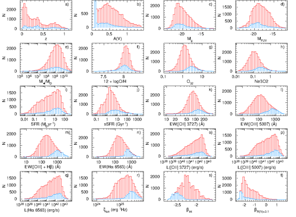
Figure 2: Histograms of the (a) redshift $z$, (b) extinction $A(V)$ in the $V$ band derived from the hydrogen Balmer decrement, (c) absolute $g$-band magnitude $M_{g}$ corrected for the Milky Way extinction, (d) ‘observed’ absolute FUV magnitude $M_{\rm FUV}$, i.e. the absolute magnitude derived from the extrapolation of the extinction-corrected SDSS spectrum and attenuated adopting extinction $A(V)$ obtained from the Balmer hydrogen decrement, (e) stellar mass derived from the SED fitting of the extinction-corrected SDSS spectrum, (f) oxygen abundance 12 + logO/H, (g) [O iii] $\lambda$5007/[O ii] $\lambda$3727 ratio denoted as O₃₂, (h) [Ne iii] $\lambda$3868/[O ii] $\lambda$3727 ratio denoted as Ne3O2, (i) star-formation rate SFR derived from the extinction-corrected H$\beta$ luminosity, (j) specific star-formation rate sSFR = SFR/($M_{\star}$/M_⊙), (k) - (n) equivalent widths of the [O ii] $\lambda$3727, [O iii] $\lambda$5007, H$\beta$ + [O iii] $\lambda$4959 + [O iii] $\lambda$5007 and H$\alpha$ emission lines, respectively, (o) - (q) extinction-corrected luminosities of the [O ii] $\lambda$3727, [O iii] $\lambda$5007 and H$\alpha$ $\lambda$6563 emission lines, respectively, (r) ionising photon production efficiency derived from the extinction-corrected H$\beta$ luminosity and extinction-corrected monochromatic luminosity at the rest-frame wavelength of 1500$\AA$, (s) extinction-corrected UV slope derived from the modelled rest-frame SED, (t) UV slope derived from the obscured SEDs with the extinction coefficient derived from the observed Balmer decrement adopting the Cardelli et al. (1989) reddening law with $R(V)$ = 3.1. In all panels, histograms represented by the red and blue lines are for the total SDSS sample of CSFGs and for CSFGs with EW(H$\beta$) $\geq$ 100$\AA$, respectively.

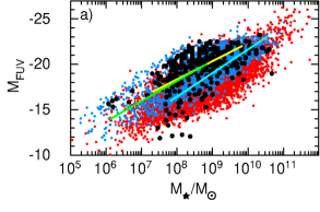
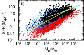
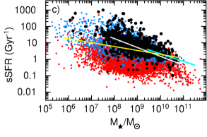
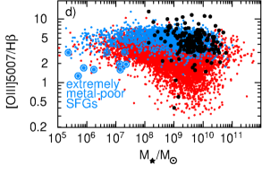
Figure 3: (a) Dependence of the FUV absolute magnitude on the stellar mass $M_{\star}$. Black-filled circles are high-$z$ galaxies (Bridge et al. 2019; Endsley et al. 2021; Karman et al. 2017; Rasappu et al. 2016; Khusanova et al. 2020; Tang et al. 2020; Strait et al. 2020b; Santos et al. 2020). Relations for high-$z$ galaxies by Song et al. (2016), Grazian et al. (2015) and Yung et al. (2019) are represented by yellow, cyan and green lines, respectively. (b), (c) SFR versus the stellar mass and the sSFR versus the stellar mass, respectively. Black-filled circles in both panels are high-$z$ galaxies (Karman et al. 2017; Amorín et al. 2016; Sanders et al. 2020a; Erb et al. 2016; Holden et al. 2016; Khusanova et al. 2020; Rasappu et al. 2016; Santos et al. 2020; Troncoso et al. 2014; Strait et al. 2020a; Reddy et al. 2006; Hagen et al. 2016; Onodera et al. 2016; Santini et al. 2017; Cullen et al. 2014; Saxena et al. 2020; Endsley et al. 2021, 2020; Tang et al. 2020; Strait et al. 2020b; Jones et al. 2020). White solid lines, yellow solid lines and cyan solid lines in (b) and (c) represent relations for high-$z$ galaxies by Arrabal Haro et al. (2020), Iyer et al. (2018) and Florez et al. (2020), respectively. (d) The dependence of the [O iii] $\lambda$5007/H$\beta$ flux ratio on the stellar mass $M_{\star}$. Black filled citcles represent high-$z$ galaxies (Richard et al. 2011; Schenker et al. 2013; Steidel et al. 2014; Troncoso et al. 2014; Holden et al. 2016). The most metal-poor nearby galaxies with 12 + log O/H $\sim$ 6.9 – 7.25 (Izotov et al. 2018c; Kojima et al. 2020, Izotov et al., in preparation) are shown by encircled blue-filled circles. The meanings of other symbols in all panels are the same as in Fig. 1.

2 Selection criteria and the sample

Our sample of CSFGs has been extracted from the spectroscopic database of the SDSS DR16 (Ahumada et al. 2020). The selection criteria are described, for example, in Izotov et al. (2016c). These criteria are as follows: (1) the angular galaxy radius on the SDSS images is $R_{50}$ $\leq$ 3 arcsec, where $R_{50}$ is the galaxy’s Petrosian radius within which 50 per cent of the galaxy’s flux in the SDSS $r$-band is contained. With this criterion, the fraction of the light outside the 3 arcsec diameter SDSS spectroscopic aperture is small. This allows us to compare SDSS spectroscopic data with photometric data in the UV, optical and infrared ranges without large aperture corrections; (2) the equivalent width of the H$\beta$ emission line is $\ga$ 10$\AA$. This criterion selects galaxies with the most extreme starbursts; (3) galaxies with AGN activity (the presence of broad Mg ii $\lambda$2800 and hydrogen emission lines, a strong high-ionisation emission line He ii $\lambda$4686 with an intensity of $\ga$ 10% that of H$\beta$ and the presence of high-ionisation [Ne v] $\lambda$3426 emission line) were excluded. Applying these criteria, $\sim$ 25000 CSFGs at redshifts $z$ $\la$ 1 were selected.

The emission-line fluxes, equivalent widths and errors were measured for each SDSS-selected spectrum, using the iraf splot routine. They were corrected for extinction from the observed decrement of all Balmer hydrogen emission lines in the SDSS spectra usable for measurements. The range of derived extinctions in our sample galaxies is discussed in Section 3.3. The procedure consists of two steps. Firstly, the emission line fluxes are corrected for the Milky Way (MW) reddening, adopting the extinction $A(V)$ from the NASA Extragalactic Database (NED) and the reddening law of Cardelli et al. (1989) with $R(V)$ = $A(V)$ / $E(B-V)$ = 3.1. This correction is applied adopting the observed wavelengths of the emission lines. Secondly, the internal extinction coefficients $C$(H$\beta$) were iteratively derived, following the prescriptions of Izotov et al. (1994), from the Balmer decrement of hydrogen emission lines, together with the equivalent widths of stellar hydrogen absorption lines, underlying the emission-line spectra. The rest-frame wavelengths of hydrogen lines and Cardelli et al. (1989) reddening law were also used. For clarity, we adopted $R(V)$ = 3.1, although Izotov et al. (2015) found that $R(V)$ = 2.7 is more likely in the far-UV range for CSFGs.

In general, the internal extinction coefficients $C$(H$\beta$) for our CSFGs are small. Therefore, the choice of the $R(V)$ value, defining the slope of the reddening law, is not important for the extinction correction in the optical range, giving small differences in the continuum and emission line fluxes for different $R(V)$s. However, it is important in the UV range. The same extinction-corrected SDSS spectra were used for the determination of some integrated characteristics, including absolute magnitudes, SFRs, $M_{\star}$s and some other characteristics (see Sect. 3.3).

3 Global characteristics of CSFGs

Here, we consider various photometric and spectroscopic charactersistics of CSFGs. As mentioned before, they are global quantities as the aperture correction is small. The characteristics directly derived from the SDSS photometric and spectroscopic data are: redshifts, luminosities, and equivalent widths of emission lines, reddening, element abundances, absolute SDSS $g$ magnitudes, and star formation rates from hydrogen emission-line luminosities.

On the other hand, fitting the spectral energy distribution with specified star-formation histories is needed for the determination of some other characteristics, such as stellar mass, specific star-formation rates, monochromatic absolute magnitudes and luminosities in the UV range, the spectral slopes in the UV range, and production efficiencies of ionising radiation $\xi_{\rm ion}$. A description of the SED modelling is given in Sect. 3.3.

3.1 Diagnostic diagrams

The BPT diagnostic diagram [O iii]$\lambda$5007/H$\beta$ – [N ii]$\lambda$6584/H$\alpha$ (Baldwin et al. 1981) for $\sim$16500 CSFGs with a measured [N ii]$\lambda$6584 emission line is shown in Fig. 1a. For the remaining $\sim$ 8500 CSFGs, that emission line is either not detected or has a redshifted wavelength outside the SDSS spectral range. It is shown in Fig. 1a that most of the CSFGs are located in the region of star-forming galaxies, below the black solid line of Kauffmann et al. (2003), which approximately separates SFGs and AGN.

A number of authors have found (e.g. Steidel et al. 2014; Shapley et al. 2015; Cullen et al. 2016; Strom et al. 2017; Bian et al. 2020) that the distribution of high-$z$ SFGs in the BPT diagram is offset from the locus of $z$ $\sim$ 0 SDSS SFGs. This difference can be caused by a combination of a harder stellar ionising radiation field, a higher ionisation parameter, and a higher N/O at a given O/H, compared to the ’plateau’ value found for local low-metallicity galaxies.

Our sample of CSFGs is shown in the BPT diagram (Fig. 1a) by red dots (galaxies with EW(H$\beta$) $<$ 100$\AA$) and blue dots (galaxies with EW(H$\beta$) $\geq$ 100$\AA$). Although this division is somewhat arbitrary, it allows us to study the properties of galaxies with different excitation conditions in their H ii regions. Furthermore, high-redshift SFGs tend to have high EW(H$\beta$) $\ga$ 100$\AA$. The galaxies from our sample with high EW(H$\beta$) occupy the upper part of the sequence for SFGs. We can see that high-EW(H$\beta$) CSFGs are offset to higher [O iii]$\lambda$5007/H$\beta$ and lower [N ii]$\lambda$6584/H$\alpha$, as compared to the total sample of SDSS SFGs (grey dots). The distribution of the latter galaxies can be approximated by the cyan line in Fig. 1a (Kewley et al. 2013). We also show the relations derived by Shapley et al. (2015) (yellow line) and by Strom et al. (2017) (green line) for $z$ $\sim$ 2 – 3 SFGs, which also fit quite well the distribution of the CSFGs in our sample with the strongest emission lines (CSFGs with EW(H$\beta$) $\geq$ 100 $\AA$, blue dots). The agreement between the locations of high-EW(H$\beta$) CSFGs and $z$ $\sim$ 2 – 3 SFGs is best seen in the inset of Fig. 1a. On the other hand, CSFGs with lower EW(H$\beta$) $<$ 100$\AA$ (red dots) are located somewhat below the relations for $z$ $\sim$ 2 – 3 SFGs (yellow and green lines), but they are still offset from the relation for the main population of $z$ $\sim$ 0 SFGs (cyan line). We conclude that the locus of CSFGs with EW(H$\beta$) $\geq$ 100$\AA$ (blue dots) and of a considerable fraction of CSFGs with EW(H$\beta$) $<$ 100$\AA$ (red dots) is similar to that of $z$ $\sim$ 2 – 3 SFGs, implying a common cause for the observed offset. One of the likely causes is the higher ionisation parameter of CSFGs and of $z$ $\sim$ 2 – 3 SFGs, compared to that of galaxies in the main sequence $z$ $\sim$ 0 sample.

We note, however, that the location of SFGs in the BPT diagram should also depend on metallicity. To illustrate this effect, we show in Fig. 1a, using encircled blue-filled circles, the sample of the most metal-deficient nearby galaxies known, with 12 + log O/H $\sim$ 6.9 – 7.25, from Izotov et al. (2018c) and Kojima et al. (2020). No galaxy with such low metallicity has been reported thus far at high redshifts. These galaxies are mostly compact and are characterised by EW(H$\beta$) $\ga$ 100$\AA$ and, thus, by high ionisation parameters, which increase from the right to the left of the BPT diagram. The most metal-deficient galaxies strongly deviate from the CSFG sequence and high-$z$ galaxies with typical 12 + log O/H $\sim$ 8.0, towards lower [O iii]$\lambda$5007/H$\beta$ ratios. It is clear that they follow a sequence that is different from those of CSFGs and $z$ $\sim$ 2 SFGs. It is likely that this sequence corresponds to galaxies at high redshifts that are least enriched with heavy elements. Therefore, the dependence on metallicity (O/H) should be taken into account in the analysis of the BPT diagram, even if N/O remains constant.

The distribution of $\sim$ 25000 CSFGs in the diagram O₃₂ = [O iii]$\lambda$5007 / [O ii]$\lambda$3727 versus R₂₃ = ([O iii]$\lambda$4959 + [O iii]$\lambda$5007 + [O ii]$\lambda$3727) / H$\beta$ is shown in Fig. 1b. The H ii regions in the galaxies from our sample are characterised by a wide range of ionisation parameter as evidenced by a large variation of O₃₂. Most of the low-EW(H$\beta$) CSFGs have low O₃₂ $\la$ 1, whereas CSFGs with EW(H$\beta$) $\geq$ 100 $\AA,$ have O₃₂ $\ga$ 1. There is a small number of CSFGs with O₃₂ $\ga$ 10, reaching in some cases extremely high values up to 60. For comparison, the relation for $z$ $\sim$ 2 - 3 SFGs by Strom et al. (2017) is also shown with a green line. It shows good agreement with the distribution of high-EW(H$\beta$) CSFGs (blue dots) and with that of a large fraction of low-EW(H$\beta$) CSFGs (red dots). This agreement implies similar properties of CSFGs and high-$z$ SFGs.

On the other hand, the most metal-deficient nearby galaxies with 12 + logO/H $\sim$ 6.9 – 7.25 and high O₃₂ $>$ 1 from Izotov et al. (2018c), Kojima et al. (2020) and Izotov et al. (in preparation) (encircled blue-filled circles in Fig. 1b) show a strong deviation from the sequences of most CSFGs and high-$z$ SFGs, indicating again a strong metallicity dependence.

Sanders et al. (2020a) and Topping et al. (2020b) considered constraints on the properties of massive stars and ionised gas for a sample of SFGs at $z$ $\sim$ 2.3. Oxygen abundances in the Sanders et al. (2020a) sample were derived by the direct $T_{\rm e}$ method and range from 12 + log O/H $\sim$ 7.5 to 8.2, whereas Topping et al. (2020b) derived 12 + log O/H $\sim$ 8.1 – 8.6 using the strong-line method. They concluded that high-$z$ SFGs differ from the local main-sequence galaxies by considerably harder ionising spectra at fixed oxygen abundance, resulting in the offset in the BPT diagram to higher [O iii]$\lambda$5007/H$\beta$ values. They also found that stellar models with super-solar O/Fe ratios and binary evolution of massive stars are required to reproduce the observed strong-line ratios in high-$z$ SFGs.

3.2 Dependence of [O/Fe] on oxygen abundance

In Fig. 1c, we show the dependence of [O/Fe] on 12 + log O/H for the CSFGs in the SDSS. We note that iron abundances are derived directly from SDSS spectra, using the [Fe iii]$\lambda$4658 and 4986 emission lines. This is different from the Sanders et al. (2020a) and Topping et al. (2020b) data, where iron abundances are derived indirectly from stellar models. The fact that our oxygen and iron abundances are derived directly from observations also means that our [O/Fe] values may be subject to the depletion of iron and oxygen onto dust grains.

We confirm the steady increase of [O/Fe] with increasing 12 + log O/H found previously, for instance, by Izotov et al. (2006) for a smaller sample of nearby SFGs. Our values of [O/Fe] are in the range $\sim$ 0.4 – 1.0 for a range of oxygen abundances 12 + log O/H $\sim$ 8.1 – 8.6, in full agreement with the values of [O/Fe] for $z$ $\sim$ 2.3 SFGs in the same range of oxygen abundances. We also note that there is no difference in distributions of CSFGs with low and high EW(H$\beta$).

Sanders et al. (2020a) found a similarly high, 3$\sigma,$ lower limit for [O/Fe] $\sim$ 0.5, but in $z$ $\sim$ 2 SFGs with lower metallicities, in apparent disagreement with our CSFGs, which have [O/Fe] $<$ 0.5 at the same lower metallicities. However, their conclusion is based on a very small sample consisting of only four galaxies. Two of these galaxies show oxygen overabundance with respect to the iron abundance, while the other two do not show this effect. Furthermore, the [O/Fe] values derived by Sanders et al. (2020a) and Topping et al. (2020b) depend on assumptions related to the star formation history and initial mass function for stars, and sets of stellar evolution models, whereas both the O and Fe abundances of our CSFGs are derived directly from observations.

The increase of [O/Fe] with 12 + log O/H likely contradicts the idea that the high [O/Fe] $\ga$ 0.5 at the highest metallicities (Fig. 1c) are due to harder radiation. In fact, we expect the ionising radiation to become harder at lower, not at higher metallicities. However, no high overabundance of oxygen relative to iron ([O/Fe] $\ga$ 0.3) is observed in CSFGs with 12 + log O/H $\la$ 7.8.

Izotov et al. (2006) have proposed an alternative explanation. They have suggested that the trend seen in Fig. 1c is not due to an oxygen overabundance, but to iron and oxygen depletion onto dust grains. That depletion is more severe at higher metallicities due to the larger content of dust. The effect is stronger for iron because it is $\sim$ 20 times less abundant than oxygen. The dust depletion hypothesis is in line with a slight increase of the noble gas neon to oxygen abundance ratio or a decrease of [O/Ne] with increasing oxygen abundance, which has been found by Izotov et al. (2006) and is shown for the CSFG sample in Fig. 1d. Therefore, it is important to increase the sample of $z$ $\sim$ 2.3 SFGs by Topping et al. (2020b) and to extend it to lower oxygen abundances to check both hypotheses.

Independently of explaining the high [O/Fe] values, we emphasise again that the distributions of high-redshift SFGs and local CSFGs in Fig. 1a - 1b are quite similar, implying similar physical properties for the galaxies in these samples.

3.3 Physical properties of CSFGs

To represent the distributions of physical properties of the CSFGs, we show in Fig. 2 histograms of various physical parameters. The histograms in red and blue are for the entire sample and for CSFGs with EW(H$\beta$) $\geq$ 100$\AA$, respectively. The redshift distribution of the galaxies is shown in Fig. 2a with three maxima at $z$ = 0.05, 0.35 and 0.8. Most CSFGs are at $z$ $\la$ 0.5, but $\sim$ 20% are at higher redshifts. Most of our CSFGs (57%) are characterised by low extinction $A(V)$ $\la$ 0.1 mag. The observed H$\alpha$/H$\beta$ ratio in a considerable number of galaxies is lower that the theoretical recombination value, mainly in objects at low redshift with high intensities of emission lines. The most likely reason for that is the clipping of emission lines, which is not rare in SDSS spectra. This effect is larger for the stronger H$\alpha$ and [O iii] $\lambda$5007 emission lines. In those cases, we adopted $A(V)$ = 0 and the intensity of [O iii] $\lambda$5007 emission line to be equal to three times the intensity of the [O iii] $\lambda$4959 emission line. The remaining galaxies (43%) are distributed over a wide range of $A(V)$ with the maximum at $\sim$ 0.45 mag (Fig. 2b).

3.3.1 Absolute magnitudes and H$\beta$ luminosity

The extinction-corrected absolute $g$-band magnitudes $M_{g}$ and extinction-corrected H$\beta$ luminosities $L$(H$\beta$) were obtained respectively from the apparent SDSS $g$-band model magnitude for the entire galaxy, corrected for Milky Way extinction, and the H$\beta$ emission-line flux measured in the SDSS spectrum and corrected for both Milky Way and internal galaxy extinction.

In principle, UV characteristics such as luminosities can be derived from the FUV and NUV magnitudes of the GALEX data base. However, CSFGs are located at very different redshifts, in the range of $z$ $\sim$ 0 – 1. Therefore, a correction for redshift is needed to derive UV magnitudes and monochromatic luminosities at fixed rest-frame wavelengths.

Instead, we decided to derive UV characteristics from the UV SEDs extrapolated from the modelled SED to the rest-frame SDSS spectrum. For the sake of comparison with high-$z$ galaxies, these SEDs are attenuated by adopting the Cardelli et al. (1989) reddening law with $R(V)$ = 3.1 and an internal extinction derived from the hydrogen Balmer decrement. Then the attenuated rest-frame SEDs are convolved with the GALEX FUV transmission curve. The details and validity of this approach have been described and justified previously, for instance, by Izotov et al. (2017a), who showed that the extrapolation of the optical SDSS SED to the UV and adopting $R(V)$ = 2.7 – 3.1 reliably reproduces the observed GALEX FUV and NUV apparent magnitudes of CSFGs. The average accuracy is better than 0.7 mag, translating to a $\sim$ 0.28 dex uncertainty in the UV luminosity and the ionising photon production efficiency $\xi_{\rm ion}$. We also note that the typical uncertainties of FUV and NUV magnitudes of CSFGs in the GALEX database are $\sim$ 0.2 – 0.4 mag. Furthermore, Izotov et al. (2016a, b, 2018a, 2018b) have shown that our procedure for extrapolating the optical SED to the UV range reproduces very well the observed HST UV spectra of $z$ $\sim$ 0.3 – 0.4 LyC leakers, which constitute a subset of our CSFG sample.

CSFGs are generally bright in both the visible and the far-UV ranges, with the absolute magnitude distributions peaking at about $-$21 mag in both wavelength ranges (Figs. 2c,d), similarly to $M_{\rm FUV}$s of the $z$ $\sim$ 2 – 8 galaxies (Bridge et al. 2019; Endsley et al. 2021; Rasappu et al. 2016; Khusanova et al. 2020; Santos et al. 2020; Song et al. 2016; Grazian et al. 2015). However, the CSFG sample shows a tail extending to very faint galaxies with $M_{g}$, $M_{\rm FUV}$ $\sim$ $-$13 to $-$14 mag. Similar low-luminosity galaxies are also present in samples of $z$ $\sim$ 3 – 6 low-luminosity galaxies (Karman et al. 2017; Song et al. 2016; Grazian et al. 2015). We also note that the distributions of $M_{g}$ and $M_{\rm FUV}$ for the entire CSFG sample (red lines in Fig. 2c,d) and for galaxies with EW(H$\beta$) $\geq$ 100$\AA$ (blue lines in Fig. 2c,d) are similar and peak at similar magnitudes.

3.3.2 Spectral energy distribution (SED) and stellar masses $M_{\star}$

The stellar mass is one of the most important global galaxy characteristics. For its determination, we follow the prescriptions described by Guseva et al. (2006, 2007) and Izotov et al. (2011, 2014). SED fits were performed for each extinction-corrected rest-frame SDSS spectrum. We take into account both stellar and ionised gas emission. The ionised gas continuum is strong in galaxies with high EW(H$\beta$) $>$ 50 $\AA$. Its contribution should be subtracted from the total SED in the determination of the stellar mass. Otherwise, stellar masses of galaxies with high EW(H$\beta$)’s in their spectra would be overestimated by a factor of $\sim$ 3 or more (Izotov et al. 2011).

Monte Carlo simulations were carried out to reproduce the stellar and nebular SEDs of each galaxy in our sample. The stellar SEDs were calculated with the PEGASE.2 package (Fioc & Rocca-Volmerange 1997) and used to derive the stellar SED of the galaxy. The star-formation history in each galaxy has been approximated by a recent short burst with age $t_{b}$ $<$ 10 Myr and a prior continuous star formation with a constant SFR between ages $t_{c1}$ and $t_{c2}$ for the older stars (Izotov et al. 2011, 2014). Furthermore, a stellar initial mass function with a Salpeter slope, an upper mass limit of 100 M_⊙, and a lower mass limit of 0.1 M_⊙ was adopted. The SED of the gaseous continuum includes hydrogen and helium free-bound, free-free, and two-photon emission (Aller 1984). The fraction of the gaseous continuum in the total SED is defined by the ratio between EW(H$\beta$)_rec for pure gaseous emission and the observed EW(H$\beta$)_obs value. The EW(H$\beta$)_rec varies in the range of $\sim$ 900 – 1100$\AA$ and also depends on the electron temperatures $T_{\rm e}$ = 10000 – 20000K, where $T_{\rm e}$ is derived from the observed spectrum.

The best modelled SED was found from $\chi^{2}$ minimisation of the deviation between the modelled and the observed continuum, varying $t_{b}$, $t_{c1}$, $t_{c2}$ and the ratio of masses of young to old stellar populations. Additionally, the best model should also reproduce the observed equivalent widths of the H$\beta$ and H$\alpha$ emission lines. Typical stellar mass uncertainties for our sample galaxies are $\sim$ 0.1 – 0.2 dex.

The distributions of stellar masses $M_{\star}$ for the entire CSFG sample and for the subsample of CSFGs with EW(H$\beta$) $\geq$ 100 $\AA$, both with their maxima at $\sim$ 10⁹ M_⊙, are shown in Fig. 2e. The mass range covered by our sample overlaps with the stellar masses currently observed in many high-redshifts studies (e.g. Holden et al. 2016; Reddy et al. 2018; Tang et al. 2020; Endsley et al. 2021). We note that the number of galaxies with stellar masses $>$ 10⁹ M_⊙ decreases, likely due to the adopted selection criteria. Many massive galaxies do not satisfy the compactness criterion.

3.3.3 Oxygen abundances 12 + log O/H

One of the most reliable methods for oxygen abundance determination is the $T_{\rm e}$-method, based on the electron temperature derived from the ([O iii] $\lambda$4959 + $\lambda$5007) / [O iii] $\lambda$4363 flux ratio. However, it requires the measurement of the weak [O iii] $\lambda$4363 flux with good accuracy. In this study, we could apply the $T_{\rm e}$-method to $\sim$ 2300 galaxies, with [O iii] $\lambda$4363 emission-line fluxes in their SDSS spectra measured with an accuracy better than 4$\sigma$. We use equations from Izotov et al. (2006) for the determination of electron temperatures, electron number densities, ionic and total oxygen, and other element abundances.

However, the SDSS spectra of most CSFGs are noisy, preventing us from applying the $T_{\rm e}$-method to derive oxygen abundances in these galaxies. Thus, for these galaxies, we resort to strong emission line (SEL) methods, with the use of strong [O ii] $\lambda$3727, [O iii] $\lambda$4959, [O iii] $\lambda$5007 and [N ii] $\lambda$6584 emission lines to derive oxygen abundances.

For the determination of the oxygen abundance in galaxies where the $T_{\rm e}$-method cannot be applied, we use the relation given by Izotov et al. (2015):

$$12+\log\frac{\rm O}{\rm H}=8.59\pm 0.02-(0.28\pm 0.01)\times{\rm O3N2},$$ (1)

where O3N2 = log ([O iii] 5007/H$\beta$) – log ([N ii] 6584/H$\alpha$). This calibration was obtained from the relation between O3N2s and oxygen abundances derived by the direct $T_{\rm e}$-method for a large sample of SDSS low-metallicity CSFGs, in which the [O iii]$\lambda$4363$\AA$ flux is derived with good accuracy. This calibration is very similar to that obtained by Pettini & Pagel (2004) who used the same relation between O3N2s and oxygen abundances derived by the direct $T_{\rm e}$-method, but for a different sample.

However, the [N ii] $\lambda$6584 emission line in faint SDSS CSFGs is weak and cannot be measured in many cases. Furthermore, this line is outside the spectral range for galaxies with $z$ $\ga$ 0.4 in earlier SDSS releases (DR1 – DR9), and for galaxies with $z$ $\ga$ 0.55 in later SDSS releases (DR10 – DR16). For these galaxies we use another calibration by Izotov et al. (2015):

$$12+\log\frac{\rm O}{\rm H}=8.18\pm 0.01-(0.43\pm 0.03)\times\log{\rm O}_{32}.$$ (2)

Equations 1 and 2 are compatible because both calibrations were based on samples with oxygen abundances derived by the $T_{\rm e}$-method.

The distributions of oxygen abundances 12 + logO/H are shown in Fig. 2f. We note that these distributions are relatively narrow, with maxima at 12 + logO/H $\sim$ 8.0 and with similar FWHMs of $\sim$ 0.3 dex for both the entire and high-EW(H$\beta$) galaxy samples.

3.3.4 O₃₂ and Ne3O2

The parameters O₃₂ and Ne3O2 defined as the [O iii]$\lambda$5007/[O ii]$\lambda$3727 and [Ne iii]$\lambda$3868/[O ii]$\lambda$3727 ratios, respectively, trace the ionisation parameter (e.g. Stasińska et al. 2015). Alternatively, these ratios are expected to be higher in density-bounded H ii regions. The distributions of O₃₂ and Ne3O2 are shown in Figs. 2g – 2h. They have maxima at O₃₂ $\sim$ 1 and Ne3O2 $\sim$ 0.1 for the entire sample. However, for galaxies with EW(H$\beta$) $\geq$ 100$\AA$, these maxima are at considerably higher values, $\sim$ 3 and $\sim$ 0.3, respectively. These differences can be due to the younger starburst age of high-EW(H$\beta$) galaxies and thus to higher luminosities of ionising radiation. Furthermore, H ii regions powered by younger bursts are likely more compact, again implying a higher ionisation parameter. The O₃₂ ratios for CSFGs are similar to those found in high-$z$ galaxies by Troncoso et al. (2014), Cullen et al. (2014), Erb et al. (2016), and Onodera et al. (2016).

Table 1: Relations between global parameters for CSFGs

$x$	$y$	Expression	Note
log (SFR-0.5$M_{\star}$/M⊙)	12+logO/H	$y$=(0.13$\pm$0.03)$x$+(6.87$\pm$0.12)	Fig. 4b
log (SFR-0.9$M_{\star}$/M⊙)	log O32	$y$=$-$(0.42$\pm$0.03)$x$+(3.78$\pm$0.24)	Fig. 5b
log EW([O ii] 3727)	log ($M_{\star}$/M⊙SFR-0.9)	$y$=$-$(2.02$\pm$0.23)$x$+(12.60$\pm$0.64)	Fig. 6b
log EW([O iii] 5007)	log ($M_{\star}$/M⊙SFR-0.9)	$y$=$-$(1.05$\pm$0.06)$x$+(10.98$\pm$0.09)	Fig. 6d
log EW(H$\alpha$ 6563)	log ($M_{\star}$/M⊙SFR-0.9)	$y$=$-$(1.10$\pm$0.09)$x$+(11.26$\pm$0.18)	Fig. 6f
log EW([O iii] 5007)	log O32	$y$=(0.56$\pm$0.06)$x$$-$(1.08$\pm$0.09)	Fig. 7a
log EW([O iii] 5007)	log Ne3O2	$y$=(0.71$\pm$0.07)$x$$-$(2.52$\pm$0.14)	Fig. 7b
log O32	log Ne3O2	$y$=(1.22$\pm$0.03)$x$$-$(1.14$\pm$0.07)	Fig. 8b
log EW([O iii] 5007)	log [(10-9$M_{\star}$/M⊙)-0.9SFR]	$y$=(0.95$\pm$0.09)$x$$-$(1.76$\pm$0.10)	Fig. 9b
log EW(H$\alpha$ 6563)	log [(10-9$M_{\star}$/M⊙)-0.9SFR]	$y$=(1.40$\pm$0.09)$x$$-$(2.90$\pm$0.18)	Fig. 9d
log EW([O iii] 5007)	log sSFR	$y$=(1.06$\pm$0.10)$x$$-$(1.96$\pm$0.17)	Fig. 10a
log EW(H$\alpha$ 6563)	log sSFR	$y$=(1.30$\pm$0.14)$x$$-$(2.68$\pm$0.24)	Fig. 10c
log EW([O iii] 5007)	log [(10-9$M_{\star}$/M⊙)0.1sSFR]	$y$=(1.01$\pm$0.09)$x$$-$(1.84$\pm$0.15)	Fig. 10b
log EW(H$\alpha$ 6563)	log [(10-9$M_{\star}$/M⊙)0.1sSFR]	$y$=(1.20$\pm$0.12)$x$$-$(2.53$\pm$0.21)	Fig. 10d
log (SFR-0.9$M_{\star}$/M⊙)	log $\xi_{\rm ion}$	$y$=$-$(0.70$\pm$0.09)$x$+(31.16$\pm$2.10)	Fig. 11b
log EW([O iii] 5007)	log $\xi_{\rm ion}$	$y$=(0.50$\pm$0.12)$x$+(23.95$\pm$0.96)	Fig. 12a
log EW(H$\alpha$ 6563)	log $\xi_{\rm ion}$	$y$=(0.80$\pm$0.09)$x$+(23.28$\pm$0.75)	Fig. 12b

3.3.5 The SFR and sSFR

The star formation rate is obtained from the extinction-corrected H$\beta$ luminosity $L$(H$\beta$) using the relation of Kennicutt (1998) between the SFR and the H$\alpha$ luminosity and adopting an H$\alpha$/H$\beta$ ratio of 2.8:

$${\rm SFR}=2.21\times 10^{-41}L({\rm H}\beta),$$ (3)

where $L$(H$\beta$) is in erg s^-1 and SFR is in M_⊙ yr^-1. Correspondingly, the specific star formation rate is determined as sSFR = SFR/$M_{\star}$.

The distribution of SFRs ranging from $\sim$ 0.01 M_⊙ yr^-1 to $\sim$ 200 M_⊙ yr^-1, which is similar to values for high-$z$ SFGs, is represented in Fig. 2i with a maximum at $\sim$ 20 M_⊙ yr^-1 for both the entire and high-EW(H$\beta$) samples. These SFRs offer a sufficient comparison with those of $\sim$ 0.1 – 100 M_⊙ yr^-1 found for high-$z$ SFGs by Holden et al. (2016), Reddy et al. (2018), Tang et al. (2020), and Endsley et al. (2021).

The distributions of sSFGs are shown in Fig. 2j with maxima at $\sim$ 2 Gyr^-1 and $\sim$ 5 Gyr^-1 for the entire and high-EW(H$\beta$) samples, respectively. Again, these values are typical of high-$z$ SFGs (e.g. Rasappu et al. 2016; Reddy et al. 2018; Cohn et al. 2018).

3.3.6 Equivalent widths and luminosities of emission lines

The distributions of EW([O ii]$\lambda$3727), EW([O iii]$\lambda$5007), EW([O iii]$\lambda$4959+5007 + H$\beta$), and EW(H$\alpha$) are shown in Figs. 2k – 2n. We display these distributions because the equivalent widths of strong emission lines are commonly reported for high-$z$ SFGs, and among them EW([O iii]$\lambda$5007) and EW(H$\alpha$) are most often used. Sometimes the EW([O iii]$\lambda$4959+5007 + H$\beta$)s are measured in low-resolution spectra, for instance, in HST prism spectra, where the [O iii] and H$\beta$ lines are not resolved.

The maxima for the high-EW(H$\beta$) sample occur at considerably higher EW values, compared to the entire sample, as expected. In particular, the values of EW([O iii]$\lambda$5007) and EW(H$\alpha$) at the maxima for CSFGs with EW(H$\beta$) $\geq$ 100$\AA$ are $\sim$ 700$\AA$ and $\sim$ 600$\AA$, respectively, with a considerable number of galaxies with EWs $>$ 1000$\AA$. On the other hand, the EWs at the maxima of the distributions for the entire sample are around four to five times lower. The smallest difference between the two samples is found for the distributions of EW([O ii]$\lambda$3727) with an EW maximum for high-EW(H$\beta$) galaxies that is only $\sim$ 30% higher than that for the entire sample. This is because the [O ii]$\lambda$3727/H$\beta$ flux ratio, in contrast to the [O iii]$\lambda$5007/H$\beta$ ratio, decreases with increasing EW(H$\beta$) and thus EW([O ii]$\lambda$3727) increases with EW(H$\beta$) more slowly than EW([O iii]$\lambda$5007). The distributions of extinction-corrected luminosities $L$([O ii]$\lambda$3727), $L$([O iii]$\lambda$5007), and $L$(H$\alpha$) are shown in Figs. 2o – 2q.

3.3.7 Ionising photon production efficiencies $\xi_{\rm ion}$

The CSFGs in our sample are characterised by high H$\beta$ and H$\alpha$ luminosities (e.g. Fig. 2q) and thus they produce copious amounts of ionising photons, which can be estimated by the production rate $N$(LyC) of the LyC radiation according to Storey & Hummer (1995):

$$N({\rm LyC})=2.1\times 10^{12}L({\rm H}\beta),$$ (4)

where $N$(LyC) and the extinction-corrected H$\beta$ luminosity $L$(H$\beta$) are in units of photons s^-1 and erg s^-1, respectively. Another parameter characterising ionising radiation is the ionising photon production efficiency, $\xi_{\rm ion}$, determined as

$$\xi_{\rm ion}=\frac{N({\rm LyC})}{L_{\nu}},$$ (5)

where $L_{\nu}$ in erg s^-1 Hz^-1 is the intrinsic monochromatic luminosity at the rest-frame wavelength of 1500$\AA,$ including the stellar and nebular emission, derived from the SED fitting. The production efficiency $\xi_{\rm ion}$ depends on metallicity, star-formation history, age of the stellar population, and also on assumptions on stellar evolution. It is higher for galaxies with higher EW(H$\beta$), that is, for younger bursts of star formation.

The distribution of $\xi_{\rm ion}$ is shown in Fig. 2r, with values varying over two orders of magnitude for the entire sample. The range of $\xi_{\rm ion}$ for CSFGs with EW(H$\beta$) $\geq$ 100$\AA$ is much narrower, and almost all galaxies from this smaller sample are above the canonical value log ($\xi_{\rm ion}$/[Hz erg^-1]) $\ga$ 25.2 – 25.3 required for the reionisation of the Universe, assuming a typical LyC escape fraction of 10 – 20% (Robertson et al. 2013; Bouwens et al. 2015).

3.3.8 Slope $\beta$ of the UV continuum

We define the slopes $\beta_{\rm int}$ and $\beta$ of the modelled intrinsic and obscured SEDs as

$$\beta_{\rm int}=\frac{\log I(\lambda_{1})-\log I(\lambda_{2})}{\log\lambda_{1}-\log\lambda_{2}},$$ (6)

$$\beta=\beta_{\rm int}-0.4\times\frac{A(\lambda_{1})-A(\lambda_{2})}{\log\lambda_{1}-\log\lambda_{2}},$$ (7)

respectively, where $\lambda_{1}$ =1300$\AA$ and $\lambda_{2}$ = 1800$\AA$ are the rest-frame wavelengths, $I(\lambda)$ is the intrinsic flux, which includes both the stellar and nebular emission, and $A(\lambda)$ is the extinction in mags.

The distribution of the intrinsic UV slope $\beta_{\rm int}$ is shown in Fig. 2s. As expected, the slopes of the younger bursts in CSFGs with EW(H$\beta$) $\geq$ 100$\AA$ are steeper, with a maximum of the distribution at $\sim$ $-2.55$ and covering the narrow range between $-2.75$ and $-2.3$. The maximum of the distribution for the entire sample is at $\sim$ $-2.3$ and the range of $\beta_{\rm int}$ variations is much larger, between $-2.75$ and $-1.7$.

For the sake of comparison with the observed UV slopes for high-$z$ SFGs, we show in Fig. 2t the distributions of obscured UV slopes of CSFGs derived from the intrinsic UV slopes. The extinction is derived from the hydrogen Balmer decrement in the SDSS spectra, assuming the reddening law by Cardelli et al. (1989) with $R(V)$ = 3.1. The $\beta$ distribution of CSFGs in the entire sample, in the range of $\sim$ –2.5 - 0.0, is similar to that for high-$z$ SFGs (see Sect. 4.5).

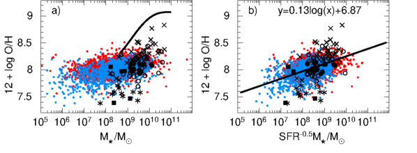
Figure 4: Dependences of oxygen abundances 12 + logO/H on (a) stellar masses $M_{\star}$ and on (b) SFR^-0.5$M_{\star}$ for the samples of CSFGs and high-$z$ SFGs. The maximum likelihood relation to SDSS data in (b) is shown by the straight solid line. The black line in (a) is the relation for $z$ = 0 SDSS SFGs by Mannucci et al. (2010). Large symbols represent high-$z$ SFGs by Amorín et al. (2016) ($z$ = 2.4–3.5, asterisks), Erb et al. (2016) ($z$ $\sim$ 2.3, filled circles), Troncoso et al. (2014) ($z$ $\sim$ 3–5, open circles), Onodera et al. (2016) ($z$ $\sim$ 3 – 3.7, crosses), Cullen et al. (2014) ($z$ $>$ 2, open triangles) and Jones et al. (2020) ($z$ = 7.1 – 9.1, filled squares). The meanings of symbols for SDSS CSFGs in both panels are the same as in Fig. 1.

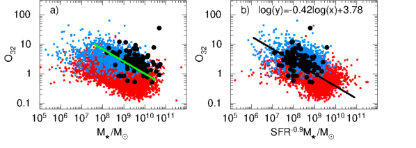
Figure 5: Dependences of O₃₂ = [O iii] $\lambda$5007/[O ii] $\lambda$3727 emission line ratios on (a) stellar masses $M_{\star}$ and on (b) SFR^-0.9$M_{\star}$ for samples of CSFGs and high-$z$ SFGs. The black line in (b) is the maximum likelihood relation whereas the green line in (a) is the relation for $z$ $\sim$ 1.7 – 3.6 galaxies (Sanders et al. 2020a). Black-filled circles represent high-$z$ SFGs by Erb et al. (2016) ($z$ $\sim$ 2.3), Onodera et al. (2016) ($z$ $\sim$ 3 – 3.7), Troncoso et al. (2014) ($z$ $\sim$ 3 – 5), and Cullen et al. (2014) (stacks of $z$ $>$ 2 galaxies). The meaning of symbols for our SDSS are the same as in Fig. 1.

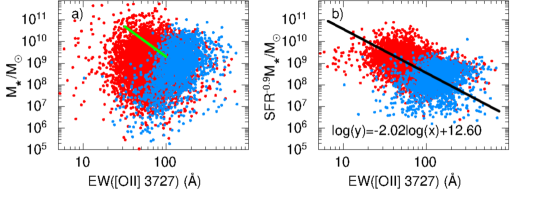
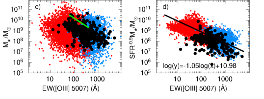
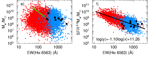
Figure 6: Dependences of stellar masses $M_{\star}$ ((a), (c), (e)) and of SFR^-0.9$M_{\star}$ ((b), (d), (f)) on the equivalent widths of the [O ii] $\lambda$3727, [O iii] $\lambda$5007 and H$\alpha$ $\lambda$6563 emission lines, respectively, for samples of CSFGs and high-$z$ SFGs. The solid lines in (b), (d), (f) are the maximum likelihood relations, whereas green lines in (a), (c), (e) are relations for $z$ $\sim$ 1.4 – 3.8 SFGs (Reddy et al. 2018). Galaxies denoted in (c) and (d) by black-filled circles are $z$ $\sim$ 3.5 LBGs (Holden et al. 2016), $z$ $\sim$ 2 SFGs (Hagen et al. 2016), $z$ $\sim$ 1.3 – 3.7 galaxies with high EW([O iii] + H$\beta$) (Tang et al. 2020), $z$ $\sim$ 7 SFGs with high EW([O iii] + H$\beta$) (Endsley et al. 2021), $z$ $\sim$ 6.6 SFGs with Ly$\alpha$ emission (Endsley et al. 2020) and $z$ $\sim$ 8 galaxies (De Barros et al. 2019). Galaxies represented in (e) and (f) by black-filled circles are $z$ $\sim$ 5 SFGs by Rasappu et al. (2016). The meanings of symbols for our SDSS CSFGs are the same as in Fig. 1.

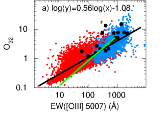
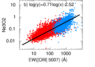
Figure 7: Relations between equivalent widths of the [O iii] $\lambda$5007 emission line and extinction-corrected (a) O₃₂ = [O iii] $\lambda$5007/[O ii] $\lambda$3727 and (b) Ne3O2 = [Ne iii] $\lambda$3868/[O ii] $\lambda$3727 for samples of CSFGs and high-$z$ SFGs. The solid lines are the maximum likelihood relations, whereas the green line in (a) is the relation for $z$ $\sim$ 1.4 – 3.8 galaxies (Reddy et al. 2018). LAEs at $z$ $\sim$ 3 by Nakajima et al. (2020) are shown in (a) by filled black circles. The meanings of symbols for SDSS CSFGs are the same as in Fig. 1.

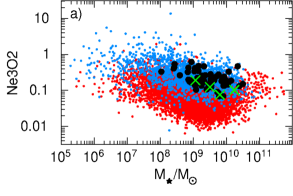
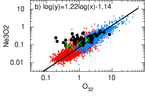
Figure 8: Dependences of Ne3O2 = [Ne iii] $\lambda$3868/[O ii] $\lambda$3727 on (a) stellar masses $M_{\star}$ and (b) the O₃₂ = [O iii] $\lambda$5007/[O ii] $\lambda$3727. The solid line in (b) is the maximum likelihood relation. The individual $z$ $\sim$ 2 SFGs from the MOSDEF survey and stacks of MOSDEF spectra from Jeong et al. (2020) are shown by black-filled circles and green crosses, respectively. The meanings of symbols for CSFGs are the same as in Fig. 1.

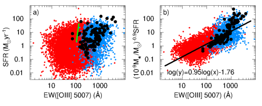
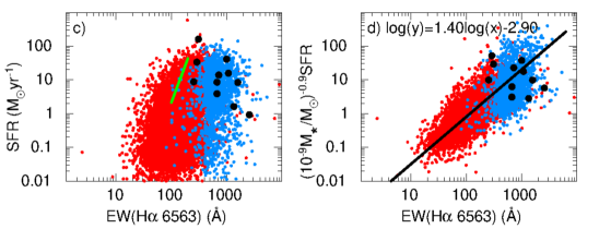
Figure 9: Dependences of star-formation rates SFR ((a), (c)) and of $M_{\star}^{-0.9}$SFR ((b), (d)) on equivalent widths of the [O iii] $\lambda$5007 and H$\alpha$ $\lambda$6563 emission lines, respectively, for samples of CSFGs and high-$z$ SFGs. The solid lines in (b) and (d) are the maximum likelihood relations. Galaxies denoted in (a) and (b) by black-filled circles are $z$ $\sim$ 3.5 LBGs by Holden et al. (2016), $z$ $\sim$ 1.3 – 3.7 galaxies with high EW([O iii] + H$\beta$) by Tang et al. (2020), $z$ $\sim$ 7 galaxies with high EW([O iii] + H$\beta$) by Endsley et al. (2021) and $z$ $\sim$ 6.6 galaxies with Ly$\alpha$ emission by Endsley et al. (2020), respectively. Galaxies represented in (c) and (d) by black-filled circles are $z$ $\sim$ 5 SFGs by Rasappu et al. (2016). Green lines in (a) and (c) are the relations for $z$ = 1.4 – 3.8 SFGs (Reddy et al. 2018). The meanings of symbols for SDSS CSFGs are the same as in Fig. 1.

4 Relations between global parameters for CSFGs and their comparison with those of high-redshift SFGs

In this section we consider relations between the global parameters of CSFGs, such as UV luminosities, stellar masses, metallicities, star formation rates, specific star-formation rates sSFRs, O₃₂ and Ne3O2 ratios, equivalent widths EW([O ii] $\lambda$3727), EW([O iii] $\lambda$5007), and EW(H$\alpha$ $\lambda$6563), ionising photon production efficiencies, and the slopes of the UV continua. We also study whether the above-mentioned parameters depend only on a single observationally accessible quantity or whether a second one is also required, similarly to the fundamental stellar mass and metallicity relation considered, for example, by Mannucci et al. (2010, see also Sect. 1). Finally, we compare these relations with the corresponding ones for high-redshift SFGs. The expressions of the relations for CSFGs discussed in this Section are summarised in Table 1 and the corresponding figures are introduced below.

4.1 Rest-frame UV absolute magnitudes, stellar masses, and star formation rates

The relations between the rest-frame UV absolute magnitudes, stellar masses, and star formation rates for high-redshift SFGs have been considered in many papers. Karman et al. (2017) found that low-mass galaxies at 3 $<$ $z$ $<$ 6 are forming stars at higher rates than seen locally or in more massive galaxies. Arrabal Haro et al. (2020) found that LAEs are typically young low-mass galaxies undergoing one of their first bursts of star formation.

It was found that the sSFR in SFGs with 2.5 $<$ $z$ $<$ 4 is 4.6 Gyr^-1 (Cohn et al. 2018) and that it increases with redshift from $z$ = 2 to 7 (sSFR $\propto$ (1 + $z$)^1.1, Davidzon et al. 2018). Tang et al. (2020) concluded that a significant fraction of the early galaxy population should be characterised by large sSFRs ($>$ 200 Gyr^-1) and low metallicities ($<$ 0.1 $Z_{\odot}$).

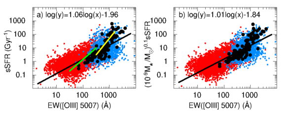
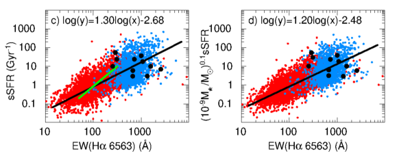
Figure 10: Dependences of specific star-formation rates sSFR ((a), (c)) and of $M_{\star}^{-0.1}$sSFR ((b), (d)) on equivalent widths of the [O iii] $\lambda$5007 and H$\alpha$ $\lambda$6563 emission lines, respectively, for samples of CSFGs and high-$z$ SFGs. Solid lines are the maximum likelihood relations. Galaxies denoted in (a) and (b) by black-filled circles are $z$ $\sim$ 3.5 LBGs by Holden et al. (2016), $z$ $\sim$ 1.3 – 3.7 galaxies with high EW([O iii] + H$\beta$) by Tang et al. (2020), $z$ $\sim$ 7 galaxies with high EW([O iii] + H$\beta$) by Endsley et al. (2021) and $z$ $\sim$ 6.6 galaxies with Ly$\alpha$ emission by Endsley et al. (2020). Galaxies represented in (c) and (d) by black-filled circles are $z$ $\sim$ 5 SFRs by Rasappu et al. (2016). Yellow and green solid lines in (a) represent relations of $z$ $\sim$ 2 analogues for $z$ $>$ 6.5 galaxies (Du et al. 2020) and $z$ = 1.4 – 3.8 SFGs (Reddy et al. 2018), respectively, whereas the relation for $z$ = 1.4 – 3.8 SFGs (Reddy et al. 2018) in (c) is shown by the green line. The meanings of symbols for SDSS CSFGs are the same as in Fig. 1.

Song et al. (2016) found that the correlation between the rest-frame UV absolute magnitude $M_{\rm FUV}$ at 1500 $\AA$ and the logarithmic stellar mass log $M_{\star}$ for $z$ = 4 – 8 SFGs is linear. Similarly, Iyer et al. (2018) found that the relation log SFR – log $M_{\star}$ at $z$ = 6 is linear down to log $M_{\star}$/M_⊙ = 6. On the other hand, Salmon et al. (2015) found that star-forming galaxies in the Cosmic Assembly Near-infrared Deep Extragalactic Legacy Survey (CANDELS), in the redshift range of $z$ = 3.5 – 6.5, follow a nearly unevolving correlation between stellar mass and SFR that follows SFR $\sim$ M_⋆^a, with $a$ = 0.70 $\pm$ 0.21 at $z$ $\sim$ 4 and 0.54 $\pm$ 0.16 at $z$ $\sim$ 6. Similarly, Arrabal Haro et al. (2020) found that the SFR – $M_{\star}$ relation has negligible evolution from $z$ $\sim$ 4 to $z$ $\sim$ 6.

In Fig. 3a, we present the relation rest-frame absolute UV magnitude $M_{\rm FUV}$ – stellar mass $M_{\star}$ for our sample of SDSS CSFGs (red and blue dots), ranging in stellar mass from $\sim$ 10⁵ M_⊙ to $\sim$ 10¹¹ M_⊙, or over six orders of magnitude, and in UV absolute magnitude from $\sim$ –12 mag to $\sim$ –25 mag, or over five orders of magnitude in the FUV luminosity. We note that the $M_{\rm FUV}$s in Fig. 3a are attenuated magnitudes, derived from the intrinsic magnitudes and adopting extinction obtained from the hydrogen Balmer decrement in the SDSS spectra, and the Cardelli et al. (1989) reddening law with $R(V)$ = 3.1. All other symbols and lines in Fig. 3a are related to high-z SFG studies, which report ‘observed’ magnitudes, uncorrected for reddening. We can see that the locations of high-$z$ SFGs are in good agreement with the location of our CSFGs with EW(H$\beta$) $\geq$ 100$\AA$ (blue dots), indicating little variation for strongly star-forming galaxies over the redshift range of $z$ $\sim$ 0 – 8.

The relations of the SFR to stellar mass $M_{\star}$ and the sSFR to stellar mass $M_{\star}$ are shown in Figs. 3b and 3c, respectively. The SFR for CSFGs ranges over five orders of magnitude, from $\sim$ 0.001 M_⊙ yr^-1 to $\sim$ 100 M_⊙ yr^-1, whereas the sSFR can reach values of up to several hundred Gyr^-1, indicating that the major part of the stellar mass has been formed during the last $<$ 10 Myr. We see in Figs. 3b and 3c that CSFGs with EW(H$\beta$) $\geq$ 100$\AA$ and high-$z$ galaxies have very similar properties.

High sSFRs in CSFGs with EW(H$\beta$) $\geq$ 100$\AA$ are related to the presence of high-excitation H ii regions with strong [O iii]$\lambda$5007/H$\beta$ ratios (blue dots in Fig. 3d), which are similar to those in high-$z$ SFGs (black-filled circles in Fig. 3d). A remarkable feature of these CSFGs with high EW(H$\beta$) and, thus, with high-excitation H ii regions is the absence of dependence on stellar mass because of very similar metallicities (12 + logO/H $\sim$ 8.0 with a standard deviation of 0.1, Fig. 2f). To justify this conclusion, we show in Fig. 3d the most metal-poor nearby galaxies with 12 + logO/H $\sim$ 6.9 – 7.25 and similar high EW(H$\beta$)s (encircled filled circles). These galaxies strongly deviate from the sequence of CSFGs with EW(H$\beta$) $>$ 100$\AA$, as in Figs. 1a – 1b.

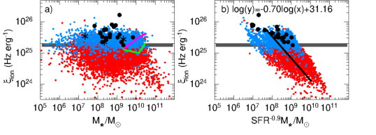
Figure 11: Relations between ionising photon production efficiences $\xi_{\rm ion}$ and stellar masses $M_{\star}$ (a) and SFR^-0.9$M_{\star}$ (b) for samples of CSFGs and high-$z$ SFGs. The solid line in (b) is the maximum likelihood relation whereas stacks for $z$ $\sim$ 1.4 – 2.6 SFGs (Shivaei et al. 2018) for Calzetti et al. (1994, 2000) and SMC reddening laws are shown in (a) by green and magenta lines, respectively. Mean $\xi_{\rm ion}$ values of $z$ = 4 – 5 galaxies (Lam et al. 2019a) in the three stellar mass bins are shown in (a) by asterisks, whereas $z$ $\sim$ 6.6 SFGs with Ly$\alpha$ emission by Endsley et al. (2020) are represented in both panels by filled circles. Values of $\xi_{\rm ion}$ assumed in canonical Universe reionisation models are shown with a thick horizontal grey line (e.g. Bouwens et al. 2016). The meanings of symbols for the SDSS CSFGs are the same as in Fig. 1.

4.2 Stellar mass and metallicity relation

A number of studies (e.g. Mannucci et al. 2010; Cullen et al. 2014; Troncoso et al. 2014; Sanders et al. 2015; Onodera et al. 2016; Curti et al. 2020; Sanders et al. 2020b) have revealed an offset of high-$z$ SFGs in the stellar mass-metallicity diagram to lower than 12 + logO/H, in the range of 0.15 – 0.70 dex, when compared to SDSS galaxies at $z$ = 0. Troncoso et al. (2014) have attributed these differences to prominent outflows and massive pristine gas inflows.

It was found in some of these studies that there is a second-order parameter in the stellar massmetallicity relation, namely the SFR, which introduces an additional scatter to the relation. We note in the introduction to this work that in Mannucci et al. (2010), by replacing the parameter log $M_{\star}$ with log $M_{\star}$ – $\alpha$ $\times$ log SFR in the fundamental mass-metallicity relation, these authors found $\alpha$ = 0.32 for a minimum of the data dispersion, whereas Curti et al. (2020) and Sanders et al. (2020a) derived $\alpha$ = 0.55 and 0.63, respectively.

The relation $M_{\star}$ – 12 + logO/H for CSFGs is represented in Fig. 4a. The oxygen abundances of 12 + logO/H were derived either by the direct $T_{\rm e}$-method for galaxies, where the [O iii] $\lambda$4363 emission line was detected with an accuracy better than 4 $\sigma$, or by the strong-line method using Eq. 1, if the [N ii] $\lambda$6584 emission line is measured, or by using Eq. 2 otherwise. Furthermore, it is only for the mass-metallicity relation, among the galaxies with oxygen abundances derived by the strong-line method, that we excluded all galaxies with [O iii] $\lambda$4959/H$\beta$ $<$ 1 because Eqs. 1 and 2 are derived using the method from Izotov et al. (2015), namely, the direct $T_{\rm e}$-method, only for galaxies with [O iii] $\lambda$4959/H$\beta$ $\geq$ 1.

The black line in Fig. 4a shows the steep relation for $z$ = 0 SDSS SFGs derived by Mannucci et al. (2010). Our shallower relation for CSFGs is offset to lower metallicities and extends to lower stellar masses. The difference is not due to a redshift effect as our galaxies are also low-redshift systems, with a major fraction below $z$ = 0.5. It is likely, as suggested by Curti et al. (2020), that at a fixed stellar mass, the requirement of an [O iii] $\lambda$4363 detection selects the most metal-poor galaxies. However, our CSFG sample includes also $\sim$ 10,000 galaxies without a detected [O iii] $\lambda$4363 emission line. These galaxies follow the same relation as those with a detected [O iii] $\lambda$4363 line (fig. 9a in Izotov et al. 2015). Possibly, the difference in the Mannucci et al. (2010) relation is caused by our selection of CSFGs with strong emission lines, whereas the Mannucci et al. (2010) sample includes many galaxies with weak emission lines and likely higher metallicities. Additionally, different methods were used in different works for oxygen abundance determination (e.g. see the discussion in Izotov et al. 2015) and the galaxies from our sample show a wider range of SFR than those in Mannucci et al. (2010), stressing the importance of this additional parameter in this relation.

For the purposes of comparison, we also show data for $z$ $\sim$ 2 – 7 galaxies in Fig. 4. They are in general agreement with the data for CSFGs but with a higher dispersion, presumably due to different methods used for oxygen abundance determination and higher uncertainties in emission fluxes for high-$z$ galaxies. To take into account the effect of the secondary parameter in the stellar mass – metallicity relation, the SFR, we show in Fig. 4b the fundamental metallicity relation 12 +log O/H – SFR^-a$\times$($M_{\star}$/M_⊙), where $a$ = 0.5 was obtained by minimising the dispersion. The linear regression of this relation and its expression are shown in the Figure. The derived value of $a$ for the CSFGs is very similar to $a$ = 0.55 obtained by Curti et al. (2020) for SDSS galaxies.

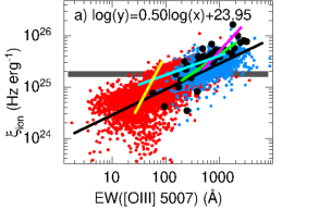
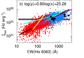
Figure 12: (a) and (b) Relations between ionising photon production efficiences, $\xi_{\rm ion}$, and equivalent widths of the [O iii] $\lambda$5007 and H$\alpha$ $\lambda$6563 emission lines for samples of CSFGs and high-$z$ SFGs. The black solid lines are the maximum likelihood relations whereas green, magenta, cyan, and yellow solid lines in (a) are the relations for $z$ $\sim$ 1.3 – 2.7 strong [O iii] emitters (Tang et al. 2019), $z$ $\sim$ 0 SFGs with EW([O iii]) $>$ 1000$\AA$ (Chevallard et al. 2018), $z$ $\sim$ 2 lensed galaxies (Emami et al. 2020), and $z$ $\sim$ 1.4 – 3.8 galaxies (Reddy et al. 2018), respectively; LAEs at $z$ $\sim$ 3 (Nakajima et al. 2020) and $z$ $\sim$ 6.6 SFGs with Ly$\alpha$ emission (Endsley et al. 2020) are shown in (a) by filled black circles. Mean $\xi_{\rm ion}$ values for $z$ = 4 – 5 galaxies (Lam et al. 2019a) are shown in (b) by filled circles. The lines in (b) are the relations for $z$ $\sim$ 1.3 – 2.7 strong [O iii] emitters (green line, Tang et al. 2019), $z$ $\sim$ 4 – 6 SFGs (magenta line, Faisst et al. 2019), $z$ $\sim$ 2 lensed galaxies (cyan line, Emami et al. 2020), and $z$ $\sim$ 1.4 – 3.8 (yellow line, Reddy et al. 2018). Values for $\xi_{\rm ion}$ assumed in canonical Universe reionisation models are shown with a thick horizontal grey line (e.g. Bouwens et al. 2016). The meanings of symbols for SDSS CSFGs are the same as in Fig. 1.

4.3 O₃₂, Ne3O2, stellar masses, and equivalent widths of emission lines

We now consider the relations between stellar masses and emission line properties for CSFGs and compare them with those for high-$z$ SFGs. Fluxes, equivalent widths of strong emission lines (EW([O ii] $\lambda$3727), and more commonly EW([O iii] $\lambda$5007) and EW(H$\alpha$)) and O₃₂ have been measured in spectra or are inferred from the photometry of many high-redshift galaxies.

In particular, Faisst et al. (2016) found that the [O iii] $\lambda$5007/H$\beta$ ratio increases progressively out to $z$ $\sim$ 6, whereas Cohn et al. (2018) concluded that extreme [O iii] $\lambda$5007 emission may be a common early lifetime phase for star-forming galaxies at $z$ $>$ 2.5. Du et al. (2020) also concluded that strong [O iii] $\lambda$4959,5007 + H$\beta$ emission appears to be typical in star-forming galaxies at $z$ $>$ 6.5. They found that extreme Ly$\alpha$ emission starts to emerge at high EW([O iii] $\lambda$5007) $>$ 1000$\AA$.

Using Spitzer photometry, Rasappu et al. (2016) derived a rest-frame EW(H$\alpha$+[N ii] + [S ii]) for $z$ = 5.1 - 5.4 galaxies of $\sim$ 700$\AA$. On the other hand, Endsley et al. (2021) studied the distribution of [O iii] + H$\beta$ line strengths at $z$ $\sim$ 7, using a sample of 22 bright ($M_{\rm FUV}$ $<$ –21 mag) galaxies, and derived a median EW = 692$\AA$ for the sum of these emission lines. Faisst et al. (2019) found a tentative anticorrelation between EW(H$\alpha$) and stellar mass, ranging from 1000$\AA$ at log($M_{\star}$/M_⊙) $<$ 10 to below 100$\AA$ at log($M_{\star}$/M_⊙) $>$ 11. Tran et al. (2020) similarly concluded that H$\beta$+[O iii] rest-frame equivalent widths in $z$ $\sim$ 3 – 4 galaxies tend to be higher in lower-mass systems. They also suggested that strong [O iii]$\lambda$5007 emission signals an early episode of intense stellar growth in low-mass galaxies and many, if not most galaxies at $z$ $>$ 3 go through this starburst phase.

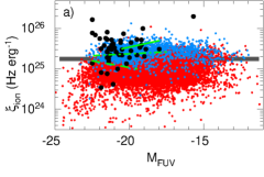
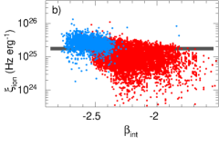
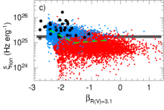
Figure 13: (a) Dependence of the ionising photon production efficiency $\xi_{\rm ion}$ on the UV absolute magnitude $M_{\rm FUV}$. The LAEs at $z$ $\sim$ 3 (Nakajima et al. 2020), $z$ $\sim$ 6.6 SFGs with Ly$\alpha$ emission (Endsley et al. 2020), mean $\xi_{\rm ion}$ values for $z$ = 3.8 – 5.4 galaxies (Bouwens et al. 2016), mean $\xi_{\rm ion}$ values for $z$ = 4 – 5 galaxies (Lam et al. 2019a), and a mean $\xi_{\rm ion}$ value for $z$ = 3.8 – 5.4 faint galaxies with high EW(Ly$\alpha$) (Maseda et al. 2020) are shown by filled circles. The relation for $\sim$ 2 galaxies (Shivaei et al. 2018), for $z$ $\sim$ 9 – 10 galaxies (Bouwens et al. 2019) and for $z$ $\sim$ 3 faint Ly$\alpha$ emitters (Nakajima et al. 2018) are shown by a green dashed, dash-dotted and solid lines, respectively. (b) Dependence of the ionising photon production efficiency $\xi_{\rm ion}$ on the intrinsic UV slope $\beta$. (c) Dependence of the ionising photon production efficiency $\xi_{\rm ion}$ on the intrinsic UV slope $\beta$ reddened with $R(V)$ = 3.1. Filled circles are $z$ $\sim$ 3.8 – 5.4 galaxies (Bouwens et al. 2016) and $z$ $\sim$ 6.6 SFGs with Ly$\alpha$ emission (Endsley et al. 2020), asterisks are mean $\xi_{\rm ion}$ values of $z$ = 4 – 5 galaxies (Lam et al. 2019a). The relation for $z$ $\sim$ 2 galaxies (Shivaei et al. 2018) is shown by a green dashed line. Values of $\xi_{\rm ion}$ assumed in canonical Universe reionisation models are shown (as in Figs. 11 and 12 in grey (e.g. Bouwens et al. 2016). The meanings of symbols for the SDSS CSFGs are the same as in Fig. 1.

Paulino-Afonso et al. (2018) studied a large sample of LAEs in the redshift range of $\sim$ 2 to 6. They found that LAEs with the highest rest-frame equivalent widths are the smallest and most compact galaxies. Finally, it was suggested that SFGs with the strongest emission lines are characterised by high O₃₂ ratios and high sSFRs, and that they may, in fact, be the main contributors to the reionisation process of the Universe (e.g. Nakajima et al. 2020).

In Fig. 5a, we show the relation between the stellar mass and the O₃₂ ratio. O₃₂ at fixed $M_{\star}$ is higher for CSFGs with high EW(H$\beta$), as expected, because the ionisation parameter is higher in younger starbursts. High-$z$ galaxies in the figure (black symbols and green line) have mainly O₃₂ $>$ 1 and are located in the region of massive CSFGs ($M_{\star}$ $>$ 10⁸ M_⊙), with high EW(H$\beta$) $\geq$ 100$\AA$. However, no low stellar mass galaxies are present in the current high-$z$ samples.

The O₃₂ ratio for CSFGs slowly increases with decreasing $M_{\star}$, attaining O₃₂ $>$ 10 in a significant fraction of galaxies with $M_{\star}$ $<$ 10⁷ M_⊙, although such high O₃₂ are present in CSFGs with stellar masses of up to 10⁹ M_⊙. This behaviour implies a dependence of the relation on a second parameter, namely, on the SFR. Introducing the parameter SFR^-a$\times$($M_{\star}$/M_⊙) instead of the stellar mass alone, we show in Fig. 5b the fundamental relation with $a$ = 0.9, where $a$ is obtained by minimising the scatter in the data. The linear regression of the fundamental relation is shown by a solid line. We note that adopting $a$ = 1 would correspond to the relation O₃₂ – sSFR^-1.

The relations between stellar mass and equivalent widths EW([O ii] $\lambda$3727), EW([O iii] $\lambda$5007), and EW(H$\alpha$) are shown in Fig. 6. As for high-$z$ galaxies, the data are available mainly for [O iii] $\lambda$5007 (black symbols in Fig. 6c,d) and, to a lesser extent for H$\alpha$, but not for [O ii] $\lambda$3727.

It is notable that there is weak correlation between EWs and the stellar mass for the entire CSFG sample (blue and red dots in Figs. 6a,c,e), whereas it is tight for high-$z$ galaxies in 6c. This can be explained by the lack of galaxies with low SFRs in the sample of high-$z$ SFGs. Figs. 6b,d,f represent the fundamental relations of EW – SFR^-a$\times$($M_{\star}$/M_⊙), with $a$ = 0.9, indicating that EWs increase with sSFRs while bearing in mind that the relation transforms to O₃₂ – sSFR^-1 if $a$ is set to 1.0.

A comparison of O₃₂ – $M_{\star}$ and EW – $M_{\star}$ relations (Figs. 5 and 6) indicates that they behave in a similar manner, namely, that both O₃₂ and EWs decrease with increasing $M_{\star}$. Moreover, both quantities increase with decreasing starburst age. Therefore, it is expected that they would tightly correlate. We show in Fig. 7a the O₃₂ - EW([O iii] $\lambda$5007) relation for CSFGs, which indeed reveals a tight correlation. We note that the distributions of high-$z$ galaxies are in agreement with this relation. The relation in Fig. 7a can be used, for example, to estimate the O₃₂ ratio and the [O ii] $\lambda$3727 line flux, if the characteristics of the [O iii]$\leavevmode\nobreak\ \lambda$5007 line (flux and equivalent width) are known.

In Fig. 7b, we present the relation between the ratio Ne3O2 = [Ne iii] $\lambda$3868 / [O ii] $\lambda$3727 and EW([O iii] $\lambda$5007) for $\sim$ 9500 CSFGs with detected [O ii] $\lambda$3727 and [Ne iii] $\lambda$3868 emission lines. This relation can be considered as an alternative to the relation in Fig. 7a. Combining the data from Fig. 7a and Fig. 7b, we find Ne3O2 = 0.089 $\times$ O₃₂. Although the [Ne iii] $\lambda$3868 emission line is around ten times weaker than the [O iii] $\lambda$5007 emission line, the relation in Fig. 7b can be useful because the Ne3O2 ratio is almost independent on uncertainties in extinction at variance to the O₃₂ ratio.

Jeong et al. (2020) considered the properties of ionised neon emission in z $\sim$ 2 SFGs drawn from the MOSFIRE Deep Evolution Field (MOSDEF) survey. They found a Ne3O2 anticorrelation with stellar mass and a considerable offset of Ne3O2 to higher values compared to $z$ $\sim$ 0 main-sequence galaxies. In Fig. 8a, we compare the location of CSFGs and $z$ $\sim$ 2 MOSDEF galaxies on the Ne3O2 – $M_{\star}$ diagram. We find that CSFGs with EW(H$\beta$) $\geq$ 100$\AA$ and $M_{\star}$ $>$ 10⁸ M_⊙ occupy the same region in the diagram as the MOSDEF galaxies (black filled circles). However, they extend to much lower stellar masses, down to 10⁶ M_⊙, and show an anticorrelation with $M_{\star}$ down to 10⁷ M_⊙. These facts imply that the ionising radiation in CSFGs and in MOSDEF SFGs, with stellar masses $M_{\star}$ $>$ 10⁸ M_⊙, shares the same properties.

Jeong et al. (2020) also found that Ne3O2 correlates positively with O₃₂ in $z$ $\sim$ 2 galaxies. Their data at a fixed O₃₂ is offset towards higher Ne3O2 when compared with local SFGs. They concluded that the ionising spectrum in $z$ $\sim$ 2 SFGs is harder compared to $z$ $\sim$ 0 galaxies resulting in stronger [Ne iii] $\lambda$3868 emission of Ne²⁺ with a high ionisation potential. In Fig. 8b, we show the relation Ne3O2 – O₃₂ for CSFGs (blue and red dots) and $z$ $\sim$ 2 MOSDEF SFGs (black-filled circles). Both Ne3O2 and O₃₂ were proposed by Levesque & Richardson (2014) as estimators for the ionisation parameter $U$ in local SFGs. Using their relations, we find that log $U$ in CSFGs (Fig. 8b) to be in the range of –3.5 to –1.5. We compare the distributions in log $U$ of the MOSDEF and CSFGs samples for O₃₂ $>$ 1, and find they are similar, again indicating close properties of ionising radiation. However, there is a considerable difference between galaxies with low-excitation H ii regions, characterised by O₃₂ $<$ 1. CSFGs follow the relation Ne3O2 $\sim$ 0.1 O₃₂, which is expected because the Ne abundance is around five to six times lower than that of oxygen (e.g. Izotov et al. 2006). On the other hand, the Ne3O2/O₃₂ ratios are $\sim$ 1 in the MOSDEF galaxies with the lowest O₃₂ $\la$ 0.3. Such high ratios are difficult to explain through stellar ionising radiation alone, even if adopting a very low stellar metallicity (Jeong et al. 2020). However, the Ne3O2/O₃₂ ratios in MOSDEF stacked spectra are very similar to those of CSFGs.

The diagrams depicting the SFR versus EW([O iii] $\lambda$5007) and EW(H$\alpha$) for the entire sample are shown in Figs. 9a and 9c, respectively. From these Figures, it is clear that correlations between these quantities for CSFGs, as well as for the high-$z$ SFGs that mainly populate the region of CSFGs with high EW(H$\beta$)s, are weak. On the other hand, tight fundamental relations are at play between $M_{\star}^{-a}$$\times$SFR and EW([O iii] $\lambda$5007) and EW(H$\alpha$) (Figs. 9b and 9d), with a high $a$ = 0.9. This indicates a strong dependence on the stellar mass $M_{\star}$. We note that a fraction of CSFGs with EW(H$\beta$) $\geq$ 100$\AA$ (in Figs. 9c,d) have EW(H$\alpha$) $\la$ 300$\AA$ because the H$\alpha$ lines in the spectra of these galaxies are clipped.

The relations in Figs. 9b and 9d with a $a$ = 1.0 would correspond to sSFR – EW([O iii] $\lambda$5007) and sSFR – EW(H$\alpha$) relations, which we consider in Figs. 10a and 10c. The fundamental relations in Figs. 10b and 10d only weakly depend on the secondary parameter $M_{\star}$, because of the small $a$ = –0.1.

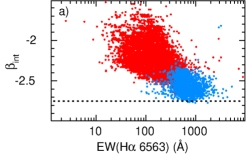
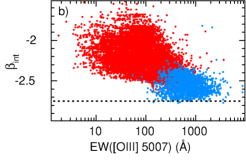
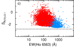
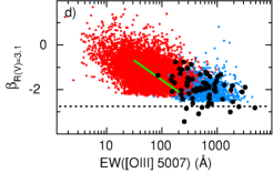
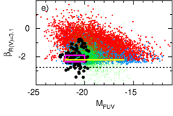
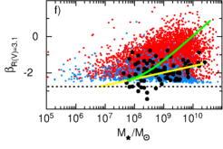
Figure 14: Dependences of the intrinsic (i.e. with zero extinction) UV SED slopes $\beta_{\rm int}$ on (a) the H$\alpha$ equivalent widths and (b) the [O iii] $\lambda$5007 equivalent widths; (c) and (d) are the same as (a) and (b), but for the SEDs reddened with the extinction coefficients derived from the hydrogen Balmer decrements and assuming the Cardelli et al. (1989) reddening law with $R(V)$ = 3.1. The green line in (d) is the relation for $z$ = 1.4 – 3.8 SFGs (Reddy et al. 2018) whereas $z$ = 3.5 LBGs (Holden et al. 2016), $z$ $\sim$ 7 galaxies with high EW([O iii] + H$\beta$) (Endsley et al. 2021) and $z$ $\sim$ 6.6 SFGs with Ly$\alpha$ emission (Endsley et al. 2020) are shown by filled circles. (e) Dependence of $\beta_{R(V)=3.1}$ on the absolute FUV magnitudes $M_{\rm FUV}$ calculated using the intrinsic SEDs. Green dots are for $z$ $\sim$ 4 – 8 SFGs (Bouwens et al. 2012, 2014), black-filled circles are for $z$ $\sim$ 6 SFGs (Pentericci et al. 2018), for $z$ $\sim$ 6.6 SFGs with Ly$\alpha$ emission (Endsley et al. 2020), for median values of $z$ $\sim$ 2 – 5 LAEs (Santos et al. 2020), for $z$ $\sim$ 7 SFGs with high EW([O iii] + H$\beta$) (Endsley et al. 2021) and for $z$ = 5.7 – 6.6 LAEs with extremely steep UV continua (Jiang et al. 2020). The magenta rectangle delineates the location of stacks for $z$ $\sim$ 10 SFGs (Wilkins et al. 2016). (f) Dependence of $\beta_{R(V)=3.1}$ on stellar masses $M_{\star}$. Black-filled circles are for $z$ $\sim$ 3.5 LBGs (Holden et al. 2016), for median values of $z$ $\sim$ 2 – 5 LAEs (Santos et al. 2020), for $z$ $\sim$ 7 SFGs with high EW([O iii]+H$\beta$) (Endsley et al. 2021), for $z$ $\sim$ 6.6 SFGs with Ly$\alpha$ emission (Endsley et al. 2020) and for stacks of SFGs at $z$ $\sim$ 4 – 6 (Fudamoto et al. 2020), respectively. Yellow solid lines in (e) and (f) represent relations for $z$ = 6 – 9 galaxies (Bhatawdekar & Conselice 2020), whereas the green solid line in (f) is the relation for $z$ = 1.5 - 3.5 LBGs by Bouwens et al. (2020). Dotted horizontal lines in all panels indicate the lowest modelled intrinsic $\beta_{\rm int}$ of –2.75. The meanings of symbols for SDSS CSFGss in all panels are the same as in Fig. 1.

4.4 Relations including the ionising photon production efficiency $\xi_{\rm ion}$

Together with the escape fraction of ionising photons from galaxies, the ionising photon production efficiency $\xi_{\rm ion}$ is one of the important parameters characterising the ability of high-$z$ SFGs to ionise the intergalactic medium during the epoch of reionisation at $z$ $\ga$ 6.

The ionising photon production efficiency $\xi_{\rm ion}$ has been derived in several studies for high-$z$ SFGs, with log($\xi_{\rm ion}$/[Hz erg^-1]) values in the range of $\sim$ 25.1 – 25.8 (Bouwens et al. 2016; Harikane et al. 2018; De Barros et al. 2019; Shivaei et al. 2018; Emami et al. 2020). On the other hand, Maseda et al. (2020) used a sample of 35 $z$ $\sim$ 4 – 5 continuum-faint LAEs and measured a very high log($\xi_{\rm ion}$/[Hz erg^-1]) = 26.28, implying a more efficient production of ionising photons in lower-luminosity Ly$\alpha$ selected galaxies, possibly produced by extremely low-metallicity stellar populations in very young starbursts. Thus, in most of these studies, the derived $\xi_{\rm ion}$s are above the canonical value required for reionising the early Universe and marked in Figs. 11 - 13 by a broad grey horizontal bar (Bouwens et al. 2016).

To better understand the contribution of dwarf galaxies to the ionising background and reionisation, Emami et al. (2020) measured the $\xi_{\rm ion}$ of low-mass galaxies (10^7.8 – 10^9.8M_⊙) in the redshift range of $1.4<z<2.7$. They do not find any strong dependence of log($\xi_{\rm ion}$) on stellar mass, far-UV magnitude, or UV spectral slope, whereas Nakajima et al. (2018) show that $\xi_{\rm ion}$ increases for fainter objects in $z$ $\sim$ 3 LAEs and Shivaei et al. (2018) derive that $\xi_{\rm ion}$ is large in galaxies with high O₃₂ ratios.

On the other hand, Emami et al. (2020), Endsley et al. (2021), Faisst et al. (2019), Tang et al. (2019), and Nakajima et al. (2020) find a correlation between log($\xi_{\rm ion}$) and the equivalent widths of H$\alpha$ and [O iii] $\lambda$5007, confirming that these quantities can be used to estimate $\xi_{\rm ion}$.

We now consider relations between $\xi_{\rm ion}$ and some global parameters of our CSFGs to check whether these relations are consistent with similar relations for high-redshift SFGs and whether the relations for low-redshift CSFGs can be used to predict $\xi_{\rm ion}$ in galaxies at any redshift.

In Fig. 11a, we present the diagram $\xi_{\rm ion}$ – $M_{\star}$ for the entire CSFG sample. Some data for high-$z$ galaxies are present as well and they are mostly located in the region of CSFGs with high EW(H$\beta$) $\geq$ 100$\AA$. A considerable fraction of our galaxies, including almost all galaxies with EW(H$\beta$) $\geq$ 100$\AA$, are characterised by high values of $\xi_{\rm ion}$, above the canonical value (Bouwens et al. 2016) shown by the grey horizontal strip. This value is suggested by models of the reionisation of the Universe. We find that no correlation exists between $\xi_{\rm ion}$ and $M_{\star}$ for the entire sample, excluding the use of stellar mass for predicting $\xi_{\rm ion}$.

However, the dispersions of the galaxy distributions in SFR bins are considerably smaller (not shown), implying a strong dependence of the $\xi_{\rm ion}$ – $M_{\star}$ relation on the secondary parameter SFR. This strong dependence is indeed seen in the fundamental relation $\xi_{\rm ion}$ – SFR^-a$M_{\star}$, with $a$ = 0.9, in Fig. 11b. Adopting $a$ = 1 would reduce the fundamental relation to $\xi_{\rm ion}$ – sSFR^-1. Thus, the relation in Fig. 11b can be used for predicting $\xi_{\rm ion}$. However, its application requires two quantities, namely, $M_{\star}$ and the SFR.

Figure 12 shows the $\xi_{\rm ion}$ – EW([O iii] $\lambda$5007) and $\xi_{\rm ion}$ – EW(H$\alpha$ $\lambda$6563) relations for the entire sample of CSFGs. For comparison, some data for high-$z$ galaxies are also included. They are in agreement with those for CSFGs. Both panels display tight correlations between $\xi_{\rm ion}$ and EW([O iii] $\lambda$5007), and EW(H$\alpha$ $\lambda$6563). The linear regressions are shown by solid black lines. Thus, both EW([O iii] $\lambda$5007) and EW(H$\alpha$) are good indicators of $\xi_{\rm ion}$ in SFGs at any redshift. In particular, $\xi_{\rm ion}$ is above the canonical value in galaxies with EW([O iii] $\lambda$5007) and EW(H$\alpha$) $\ga$ 300$\AA$ (Figs. 12a – 12b). We note, however, that we may see a considerable number of both CSFGs and high-$z$ SFGs with low EWs, but with $\xi_{\rm ion}$s above the canonical value. We attribute this result to uncertainties in EW measurements and SED modelling.

On the other hand, $\xi_{\rm ion}$ does not show any correlation with the absolute magnitude $M_{\rm FUV}$ (Fig. 13a). For comparison, we also show high-$z$ galaxy data, which are in general agreement with the data for CSFGs at the bright end of $M_{\rm FUV}$. Only two high-$z$ galaxies are outliers, located above the distribution of CSFG galaxies.

We next consider relations between $\xi_{\rm ion}$ and the intrinsic ($\beta_{\rm int}$) and obscured ($\beta_{R(V)=3.1}$) slopes of the UV continuum (Figs. 13b and 13c). As expected, almost all CSFGs with EW(H$\beta$) $\geq$ 100$\AA$ (blue dots) are located above the canonical value and the data for high-$z$ SFGs are in agreement with those for CSFGs (black symbols and the dashed green line in Fig. 13c), if the Cardelli et al. (1989) reddening law, with $R(V)$ = 3.1 and extinctions derived from the Balmer decrement, are adopted for the latter galaxies.

4.5 Relations involving the UV continuum slope $\beta$

The slope of the UV continuum (see Sect. 3.3.8) is a common characteristic derived from the photometric and spectroscopic observations of high-redshift SFGs. Thus, Bouwens et al. (2012, 2014) derived a slope $\beta$ for a large sample of $z$ $\sim$ 4 – 8 galaxies and reported a steepening of the slope at lower luminosities. These results are in agreement with what was found by Karman et al. (2017), who obtained $\beta$ $<$ –2 for all galaxies with $M_{\star}$ $<$ 10⁸ M_⊙. Bhatawdekar & Conselice (2020) obtained $\beta$ for galaxies at $z$ = 6 – 9 in the Frontier Field cluster MACSJ0416.1-2403. No correlation was seen between $\beta$ and the rest-frame UV magnitude at $\lambda$ = 1500$\AA$. Instead, they found a strong correlation between $\beta$ and stellar mass, with lower mass galaxies exhibiting bluer UV slopes, but no trend was seen between $\beta$ and sSFR. Finally, Wilkins et al. (2016) derived $\beta$ $\sim$ –1.9 - –2.3 for $z$ $\sim$ 10 galaxies.

In this section, we consider whether the UV slopes of CSFGs are consistent with those of high-redshift SFGs. Fig. 14a and 14b present the dependences of the intrinsic slope $\beta_{\rm int}$ on the rest-frame equivalent widths of the H$\alpha$ and [O iii] $\lambda$5007 emission lines. The dotted horizontal lines indicate the lowest value of $\beta$ $\sim$ –2.75, derived from the stellar continuum of the youngest bursts. We note that $\beta_{\rm int}$ attains its minimum value at EW(H$\alpha$) $\sim$ 700$\AA$ (corresponding to EW(H$\beta$) $\sim$ 200$\AA$) and then increases again at higher EW(H$\alpha$). This is caused by the contribution of nebular continuum in the UV range, characterised by a shallower slope than the stellar slope. This continuum contribution is relatively high at large EW(H$\alpha$) $\ga$ 700$\AA$ and should be taken into account (see also Raiter et al. 2010).

Figs. 14c and 14d show the obscured $\beta$s vs. the H$\alpha$ and [O iii] $\lambda$5007 equivalent widths, adopting the Cardelli et al. (1989) reddening law, with $R(V)$ = 3.1. The distribution of high-redshift SFGs in Fig. 14d is in agreement with that for CSFGs, excluding high-$z$ objects with the steepest slopes.

Similarly, there is agreement between the CSFGs and high-redshift SFGs in the diagrams of $\beta_{R(V)=3.1}$ – $M_{\rm FUV}$ and $\beta_{R(V)=3.1}$ – $M_{\star}$, respectively (Figs. 14e and 14f), excluding some high-$z$ galaxies with lowest $\beta$s. Again, this indicates an overall agreement between the properties of CSFGs and high-redshift galaxies.

5 Conclusions

In this study, we discuss the properties of a sample of $\sim$ 25,000 compact star-forming galaxies (CSFGs) at redshift $<$ 1 from Data Release 16 (DR16) of the Sloan Digital Sky survey (SDSS). The properties of the CSFGs are compared to those of star-forming galaxies at high redshift ($z$ $\ga$ 1.5), including the relations for equivalent widths of the strongest emission lines EW([O ii] $\lambda$3727), EW(H$\beta$), EW([O iii] $\lambda$5007), and EW(H$\alpha$). Our results are as follows.

1. The sample of CSFGs includes galaxies in a wide range of stellar masses from $\sim$ 10⁶M_⊙ to $\sim$ 10¹¹M_⊙ and is characterised by high star formation activity with SFR up to $\sim$ 100 M_⊙ yr^-1 and sSFR up to several hundred Gyr^-1. The equivalent widths of the strongest emission lines [O iii] $\lambda$5007 and H$\alpha$ are in excess of $>$ 1000 $\AA$ in $\sim$ 1200 galaxies.

2. Our comparison shows that the properties of our $z<1$ CSFGs are very similar to all known properties of high-redshift galaxies at $z$ $\sim$ 1.5 – 10. We find no differences between these two types of objects, indicating similar physical characteristics of massive stellar populations in these galaxies and showing CFSGs to be good local analogues of the high-redshift objects.

In conclusion, we find that CSFGs can be studied in much more detail compared to high-$z$ SFGs thanks to their proximity and the ability to characterise them based on a much wider range of physical characteristics, such as stellar masses, star formation rates, and UV luminosities. Therefore, they can be used to predict the physical properties of high-redshift galaxies to be studied by future ground-based and space telescopes, including the James Webb Space Telescope.