Spin state and moment of inertia of Venus

Fundamental properties of the planet Venus, such as its internal mass distribution and variations in length of day, have remained unknown. We used Earth-based observations of radar speckles tied to the rotation of Venus obtained in 2006–2020 to measure its spin axis orientation, spin precession rate, moment of inertia, and length-of-day variations. Venus is tilted by 2.6392 $\pm$ 0.0008 degrees ($1\sigma$) with respect to its orbital plane. The spin axis precesses at a rate of 44.58 $\pm$ 3.3 arcseconds per year ($1\sigma$), which gives a normalized moment of inertia of 0.337 $\pm$ 0.024 and yields a rough estimate of the size of the core. The average sidereal day on Venus in the 2006–2020 interval is 243.0226 $\pm$ 0.0013 Earth days ($1\sigma$). The spin period of the solid planet exhibits variations of 61 ppm ($\sim$20 minutes) with a possible diurnal or semidiurnal forcing. The length-of-day variations imply that changes in atmospheric angular momentum of at least $\sim$4% are transferred to the solid planet.

Venus is Earth’s nearest planetary neighbor and closest analog in the Solar System in terms of mass, radius, and density. However, Venus remains enigmatic on a variety of fundamental levels: the size of its core is unknown [1]; whether the core is solid or liquid is uncertain [2, 3]; and estimates of its average spin period are discordant [4, 5, 6]. Venus is also distinctive because of its 243-day retrograde rotation and 4-day atmospheric superrotation, neither of which is fully understood [7, 8, 9]. High-precision measurements of the spin state enable progress in all these areas.

The polar moment of inertia provides an integral constraint on the distribution of mass in a planetary interior, $C=\int_{V}\rho r^{2}dV$, where the volume integral includes the mass density $\rho$ at each point and the square of the distance $r$ from the spin axis. Along with bulk density, the moment of inertia is arguably the most important quantity needed to determine the internal structure of a planetary body. In particular, it can be used to place bounds on the size of the core, which is essential in understanding a planet’s thermal, spin, and magnetic evolutionary histories. Seismology, which has been conducted on Earth, Moon, and Mars, provides a powerful probe of planetary interiors, but is considered “a distant goal” at Venus [10] due to the planet’s extreme surface temperature ($\sim$740 K) and pressure ($\sim$90 atm).

Gravitational torques from the Sun result in a precession of the spin axis, which is similar to the motion of a spinning top. The rate of precession is inversely proportional to the polar moment of inertia [11]:

$$\frac{d\psi}{dt}=\frac{3}{2}\left(\frac{n^{2}}{\omega}\right)J_{2}\left(\frac{MR^{2}}{C}\right)\cos{\theta},$$ (1)

where $n$ is the orbital mean motion, $\omega$ is the spin rate, $J_{2}$ is the second-degree coefficient in the spherical harmonic expansion of the gravity field, $M$ is the mass, $R$ is the radius, and $\theta$ is the obliquity, or angular separation between spin and orbit poles. Measurements of the spin precession rates of Earth (50.2877 arcsec/y) and Mars (7.576 arcsec/y) yield $C/MR^{2}$=0.3307 [12] and $C/MR^{2}$=0.3662 [13], respectively. The predicted precession rate of Venus for a nominal $C/MR^{2}=0.336$ is $44.75$ arcsec/y, where we have used $n=585.17$ deg/y [14], $\omega=541.06$ deg/y, $J_{2}=4.40454\times 10^{-6}$ [15], and $\theta=2.639$ deg. This value is in good agreement with a previous estimate [16] and implies a precession cycle of $\sim$29,000 y.

Although the predicted precession rate of Venus is similar to that of Earth, the motion of the spin pole in inertial space is only 2.06 arcsec/y because of Venus’s small obliquity. Detection of the precession was out of reach of the 1990–1994 Magellan spacecraft mission despite its extensive radar coverage with resolution as fine as 100 m [17]. The best Magellan estimates of the spin axis orientation from analysis of radar and gravity data have uncertainties of 46 arcsec [4] and 14 arcsec [15], respectively. If a future mission were to measure the spin axis orientation with infinite precision at an epoch circa 2040, the measured precession excursion of $\sim$100 arcsec since the Magellan epoch would be determined with 14 arcsec errors at best, or 14% uncertainties, which is not geophysically useful. Likewise, if a future orbiter with 5-year duration were to measure the inertial positions of landmarks with 30 m precision, it would detect the $\sim$10 arcsec precession over the mission duration, which corresponds to a maximum displacement of $\sim$300 m, with 10% uncertainties at best. A useful measurement could be obtained with telemetry data from multiple landers, as in the case of Mars, but the technical challenge and cost of this endeavor make it improbable in the foreseeable future.

Measurements of the average spin period of Venus with $<$1% precision were first obtained by tracking the positions of surface features detectable in Earth-based radar images spanning multiple conjunctions [18, 19, 20, 21]. The most precise value to date was obtained by analyzing the positions of hundreds of landmarks detectable in Magellan spacecraft radar images recorded in the early 1990s, which resulted in a $\sim$500-day-average spin period estimate of 243.0185 $\pm$ 0.0001 days [4]. Certain features observed in Magellan images were also detected in Venus Express spacecraft images obtained circa 2007, enabling a $\sim$16-year-average spin period estimate of 243.023 $\pm$ 0.001 days [5]. Recent measurements of the positions of surface features in Earth-based radar images obtained between 1988 and 2017 yielded a $\sim$29-year-average spin period estimate of 243.0212 $\pm$ 0.0006 days [6]. None of these estimates were of sufficient precision to detect either sidereal length-of-day (LOD) fluctuations or the precession of the spin axis.

The maintenance of a 243-day retrograde spin requires explanation because solid body tides raised by the Sun would synchronize the spin of Venus to its 225-day orbital period in the absence of other forces [22, 23]. Gold and Soter [24] and others [25, 26, 27] proposed that solar torques on a thermally-induced atmospheric tide might counteract the solid-body torques and stabilize the spin. In this process, atmospheric mass decreases on the hot afternoon side of the planet and increases on the colder morning side. This imbalance creates an atmospheric bulge that leads the sub-solar point, whereas the bulge due to tides raised on the solid body lags the sub-solar point. The opposing solar torques may therefore stabilize the spin rate. The solid-body torque is relatively independent of the spin rate, but the strength of the torque on the atmospheric bulge has a semidiurnal dependence [24, 25, 26]. It is thought that the spin rate settles where the two torques balance each other. However, the magnitude of variations around the equilibrium and the nature of the response to departures from equilibrium have not been elucidated.

With a spin rate controlled by a thermally driven atmospheric tide, the rotation of the planet likely changes as a result of variations in albedo [7], orbital eccentricity [28], insolation, climate, and weather. The insolation changes by 3% as Venus revolves around the Sun with its current eccentricity of 0.007 and by 15% with the long-term average eccentricity of 0.035 [28]. The planet may therefore exhibit daily and seasonal fluctuations in LOD superposed on a complex spin rate evolution on longer timescales.

Atmospheric angular momentum (AAM) on Earth varies by tens of percent [29] and results in LOD variations on the order of milliseconds. With its massive atmosphere, Venus has an estimated AAM value ($L\sim 2.9\times 10^{28}$ kg m² s${}^{-1}\pm 30\%$) [8] that is $\sim$180 times larger than Earth’s and the atmospheric fraction of total planetary angular momentum is $\sim$60,000 larger than Earth’s. If a fraction $\epsilon$ of AAM is transferred to the solid planet, the rotation period $P$ changes by $\Delta P/P=-\epsilon L/C\omega$. For Venus, $\Delta P\simeq-9.4\epsilon$ h. Peak-to-peak estimates of AAM-induced LOD variations based on Global Circulation Model (GCM) simulations currently span at least two orders of magnitude, with values of $\epsilon$ ranging from below $\sim$0.1% [30, 31] on diurnal timescales to above $\sim$15% [32] on decadal timescales.

Observations

We obtained high-precision measurements of the instantaneous spin state of Venus with a radar speckle tracking technique that requires two telescopes and does not involve imaging (see ‘Radar speckle tracking’ in Methods). We used the 70 m antenna (DSS-14) at Goldstone, California (35.24^∘N, -116.89^∘E) and transmitted a circularly polarized, monochromatic signal at a frequency of 8560 MHz ($\lambda=3.5$ cm) and power of $\sim$200–400 kW. Radar echoes were recorded at DSS-14 and also at the 100 m Green Bank Telescope (GBT) in West Virginia (38.24^∘N, -79.84^∘E) with fast sampling systems [33].

Radar echoes from solid surfaces are speckled. The radar speckles are tied to the rotation of Venus and sweep over the surface of the Earth with a trajectory that is occasionally aligned with the two telescopes (Figs. 1 and 2). We cross-correlated the echo time series received at each telescope and obtained strong correlations that lasted $\sim$30 s (Fig. 3). The epoch at which the high correlation occurs is diagnostic of the spin axis orientation. The time lag at which the correlation maximizes yields a measurement of the instantaneous spin period.

Figure 1: Representative variations in radar echo power (speckles) from observations of Venus with the Goldstone Solar System Radar and Green Bank Telescope at 8560 MHz on 2016 Nov. 26. The GBT echo was shifted in time by 20 s to illustrate the high degree of correlation between the received waveforms when the speckle trajectory is aligned with the antenna baseline.

Figure 2: Radar echoes from Venus sweep over the surface of the Earth during the 2020 Sept. 08 observations. Diagrams show the trajectory of the speckles one hour before (left), during (center), and one hour after (right) the epoch of maximum correlation. Echoes from two receive stations (red triangles) exhibit a strong correlation when the antennas are suitably aligned with the trajectory of the speckles (green dots shown with a 1 s time interval).

Figure 3: Representative functions obtained by cross-correlating Venus radar echoes recorded at Goldstone, CA, and Green Bank, WV, on 26 Nov 2016, with Gaussian fits shown in red. (a) Time evolution of the maximum in the cross-correlation function with echo time series decimated to a sampling rate of 200 Hz. The time of the correlation maximum represents the epoch at which the speckle trajectory is aligned with both antennas and is diagnostic of spin axis orientation. (b) Cross-correlation of echo time series with 5000 Hz sampling rate and 5 ms moving average at the time of the correlation maximum shown in panel a. The time lag corresponding to the correlation maximum is diagnostic of the instantaneous spin rate. Successive measurements of this time lag yield the estimates and $\sim$5 ppm fractional uncertainties listed in Table 1.

We attempted to observe Venus on 121 instances between 2006 and 2020 (Supplementary Table LABEL:tab-all) and were successful on 21 occasions, with observing circumstances reported in Supplementary Table 2. The observing protocol and data reduction technique (see ‘Observing protocol’ and ‘Data reduction technique’ in Methods) closely followed those used for similar measurements at Mercury [34, 35] that were confirmed at the 1% level by subsequent spacecraft observations [36].

We fit Gaussians to the correlation functions in order to obtain estimates of the epochs of correlation maximum $\hat{t}$. We also obtained estimates of the time lags $\hat{\tau}$ that maximize the correlation functions (Fig. 3, Table 1). With large signal-to-noise ratios, Gaussian centroid locations can be determined with a precision that is a small fraction of the widths of the correlation functions [37]. Measurement residuals and spread in consecutive estimates suggest that epochs of correlation maxima and time lags can be determined to precisions of $\sim$0.3 s and $\sim$0.1 ms from initial widths of $\sim$10 s and $\sim$7 ms, respectively. We used the $\hat{t}$ and $\hat{\tau}$ observables to determine the instantaneous spin state of Venus (See ‘Conversion of observables to spin state estimates in Methods).

Date	Epoch (MJD)	$A$	$w$ (s)	Time lag (s)	$\epsilon$ (ppm)	$P$ (days)
060128	53763.69074757	0.593	4.70	-149.224656	6.09	243.01724
060129	53764.69293247	0.622	5.11	-142.602992	7.42	243.02106
060207	53773.69201430	0.573	6.24	-95.544513	6.57	243.01721
060214	53780.67533999	0.594	12.52	-74.199631	3.93	243.02289
060219	53785.65987182	0.696	9.66	-63.745660	4.44	243.02168
090614	54996.76400084	0.709	9.27	-20.401318	3.07	243.01596
090801	55044.63200521	0.583	13.98	-17.883815	5.76	243.01594
120310	55996.01816745	0.693	4.85	-18.228874	4.44	243.02257
120311	55997.01549785	0.615	5.32	-18.748452	3.71	243.02468
120314	56000.00753916	0.654	5.28	-20.327400	7.44	243.02073
120315	56001.00490798	0.663	5.65	-20.860567	5.54	243.01651
140312	56728.58912128	0.705	9.73	-36.100686	2.19	243.02960
140314	56730.58274410	0.764	9.81	-34.453769	2.73	243.02925
140315	56731.57957689	0.807	9.63	-33.652202	2.41	243.03075
161122	57714.87788177	0.693	12.90	-19.417283	4.60	243.02861
161125	57717.87004808	0.760	11.75	-19.821632	4.01	243.02932
161126	57718.86741525	0.779	11.45	-19.945238	3.29	243.02635
190206	58520.68253779	0.562	14.52	-21.925929	5.68	243.02289
190207	58521.67959325	0.564	14.83	-21.846558	4.72	243.02335
190208	58522.67663675	0.568	12.70	-21.759899	5.23	243.02186
200908	59100.52352634	0.497	8.02	-17.088679	4.51	243.01782

Table 1: Measurements of the instantaneous spin state of Venus. The epoch of correlation maximum is reported as a Modified Julian Date (MJD). It is the centroid of a Gaussian of amplitude $A$ and standard deviation $w$. The time lag indicates the time interval for speckles to travel from one station to the other at the corresponding epoch. The reference epochs correspond to arrival times at the GBT, and the negative lag values indicate that Venus speckles travel from west to east. The $1\sigma$ fractional uncertainty $\epsilon$ that applies to both the time lag and spin period is empirically determined from successive measurements. The last column indicates the instantaneous, sidereal spin period in Earth days, after application of small refraction corrections (Table 2).

Spin axis orientation, precession, and moment of inertia

The velocity vector of the speckle pattern lies in the plane perpendicular to the component of the spin vector that is perpendicular to the line of sight. The correlation of Goldstone and GBT radar echoes is large only when the antenna separation vector projected perpendicular to the line of sight, or projected baseline, lies in the same plane. Correlation epoch measurements provide tight constraints on the component of the spin that is perpendicular to the line of sight and loose constraints on the orthogonal component. As a result, each epoch measurement delineates a narrow error ellipse for the orientation of the spin axis on the celestial sphere. We obtained intersecting error ellipses by observing Venus at a variety of orientations (Fig. 4).

Figure 4: Constraints on the spin axis orientation of Venus obtained with Goldstone-GBT observations of radar speckles. Each colored line represents a measurement of the epoch of correlation maximum that traces a narrow error ellipse on the celestial sphere. The orientation of each line is related to the ecliptic longitude of the projected baseline at the time of observations (Supplementary Table 2). The best-fit spin axis orientation is shown by a diamond at the intersection of the colored lines. All measurements have been precessed to the J2000.0 epoch. The black dotted line represents the trace of the spin axis orientation on the celestial sphere as a result of spin precession between 1950 and 2050.

We used the epochs of correlation maxima (Table 1) with uniform uncertainties in a three-parameter least-squares fit to estimate the spin axis orientation of Venus as well as its precession rate. The first two adjustable parameters are the right ascension (RA) and declination (DEC) of the spin axis in the equatorial frame of J2000.0. The third adjustable parameter is the normalized moment of inertia $C/MR^{2}$, with precession modeled according to equation (1). Post-fit residuals have a standard deviation of 0.32 s and their distribution is unremarkable (Supplementary Fig. 1). We estimated confidence intervals with 2000 bootstrap trials, which confirmed the robustness of the fit results with respect to inclusion or exclusion of certain data points. Results are listed in Table 2.

Quantity	Least squares	Bootstrap mean	Std. dev.
RA (deg)	272.73911	272.73912	0.0008
DEC (deg)	67.15105	67.15100	0.0007
$d\psi/dt$ (′′/y)	-44.89	-44.58	3.3
$C/MR^{2}$	0.3350	0.3373	0.024
$C$ (1037 kg m2)	5.972	6.013	0.43

Table 2: Estimates of Venus spin axis orientation, precession rate, and moment of inertia from least-squares fit and bootstrap analysis. Angles refer to epoch J2000.0.

The spin axis orientation of Venus is determined with an overall precision of 2.7 arcsec, which improves upon the Magellan estimates by a factor of 5–15 (Fig. 5). At first glance, our estimates are only marginally consistent with the Magellan estimates. However, the spin axis orientation measured by Magellan in the early 1990s is not directly comparable to our solution, which has a reference epoch of J2000.0. If we use our estimate of the precession rate and precess the Magellan estimates to epoch J2000.0, we find that our values fall well within the Magellan $1\sigma$ uncertainty contours (Fig. 5).

Figure 5: Spin axis orientation of Venus shown with 1-, 2-, and 3-sigma uncertainties (2D confidence intervals at 68.3%, 95.4%, and 99.7% levels, respectively). The epoch J2000.0 solution based on Goldstone-GBT observations is shown in black. The Magellan solutions of Davies et al. [4] and Konopliv et al. [15] are shown in blue and red, respectively. The black dotted line represents the trace of the spin axis orientation on the celestial sphere as a result of spin precession between 1950 and 2050. (a) Magellan solutions as published by Davies et al. [4] and Konopliv et al. [15]. (b) Magellan solutions precessed to epoch J2000.0 from the mid-point of the corresponding observation intervals (Jan 1991 and Sep 1993, respectively).

Our improved value of the obliquity of Venus is 2.6392 $\pm$ 0.0008 deg ($1\sigma$), where we have used a recent determination of the orbital plane orientation with RA=278.007642 deg and DEC=65.566999 deg [14]. The origin and maintenance of the obliquity has been linked to planetary perturbations, core-mantle friction, and atmospheric torques [7, 38, 39]. If the core is liquid, the obliquity estimate can be used to place bounds on the viscosity or ellipticity of the core, provided that atmospheric torques are modeled accurately [7].

The distribution of normalized moments of inertia from the bootstrap analysis suggests residual uncertainties of 7% with the data obtained to date (Fig. 6). The results are not yet sufficient to rule out certain classes of interior models, whose normalized moments of inertia computed in a recent study [2] span the range 0.327 – 0.342. Nevertheless, the best-fit value of the moment of inertia factor combined with knowledge of the bulk density ($\rho$=5242.8 kg/m³) enable a crude estimate of the size of the core of Venus with a two-layer, uniform-density model (See ‘Two-layer interior structure model’ in Methods). We find a core radius of approximately 3500 km (58% of the planetary radius) with large ($>$500 km) uncertainties due to both model limitations and current uncertainties on $C/MR^{2}$.

Figure 6: A bootstrap analysis of radar speckle tracking estimates of the normalized moment of inertia of Venus suggests residual uncertainties of 7% with the data obtained to date.

Spin period and length-of-day variations

We used the time lag measurements to compute the spin period of Venus at each observation epoch (Table 1). The data show that Venus exhibits substantial LOD variations (Fig. 7). We reject the hypothesis of a constant spin period with high confidence (p-value $<<10^{-16}$) because a model with constant spin period yields a large sum of squares of residuals (SSR=620). In addition, we find that published values of Venus’s average spin rate [4, 5, 6] are inconsistent with most of our instantaneous spin period measurements.

Our data set spans almost 15 years and includes 21 measurements with an average fractional uncertainty of 5 ppm. The median value of our measurements provides a robust estimate of the average length of day on Venus, $P$=243.0226 $\pm$ 0.0013 days ($1\sigma$), where the error bars are obtained by bootstrap resampling (see ‘Estimate of average spin period’ in Methods). Natural variability around the mean is at least $\pm$ 0.0047 days ($1\sigma$). Our improved determinations of the spin axis orientation, precession rate, and spin period form the basis of a recommended orientation model for Venus (Supplementary Information). This model and the model currently in use [4] yield differences in the predicted inertial positions of equatorial landmarks that grow by $\sim 1$ km per year. Stochastic LOD variations over a 10-year period contribute an additional uncertainty of $\pm$3.3 km ($1\sigma$), which will complicate the establishment of new geodetic control networks and the measurement of the spin precession from orbital or landed platforms (Supplementary Information).

The fractional excursion in instantaneous spin rate observed to date is 61 ppm, which corresponds to variations in spin period of 0.015 days or 21 minutes. On seven instances, we observed Venus on consecutive days and measured variations ranging between 2 and 17 ppm with a weighted average value of 9 $\pm$ 5 ppm ($1\sigma$), suggesting a spin rate of change as large as $d\omega/dt\sim 3.1\times 10^{-17}$ rad s^-2 and corresponding torques $T=Cd\omega/dt\sim 1.9\times 10^{21}$ N m. The LOD variations observed at Venus are 3 orders of magnitude larger than on Earth, where core-mantle interactions can change the LOD by $\sim$4 ms (46 ppb) on $\sim$20-year timescales [40]. The torques responsible for the LOD variations on Earth are $T_{\oplus}=C_{\oplus}d\omega_{\oplus}/dt\sim 4.3\times 10^{17}$ N m, where $d\omega_{\oplus}/dt\sim 5.4\times 10^{-21}$ rad s^-2 and $C_{\oplus}=8.0\times 10^{37}$ kg m². If Venus has a liquid core, it may experience torques of the same order of magnitude, which would yield $d\omega/dt\sim 10^{-20}$ rad s^-2, a factor of $10^{3}$ too small compared to observations. Tidal despinning torques are an order of magnitude smaller. We conclude that changes in AAM are primarily responsible for the LOD variations at Venus. Other contributions to the LOD variations include a $\sim$3 ppm variation at semidiurnal frequencies due to solar torques on Venus’s permanent deformation and possibly sub-ppm variations due to core-mantle interactions [31]. The AAM variations are so large that they likely prevent capture in resonances with Earth, a phenomenon that has been hypothesized for decades [41, 25, 7, 28].

Figure 7: (a) Measurements of the instantaneous spin period of Venus shown as blue dots with $1\sigma$ error bars. These data are based on time lag measurements of radar speckles observed with Goldstone and the GBT between 2006 and 2020. Horizontal lines and shaded areas show the average spin periods derived from Magellan radar images (1990–1992, orange), Magellan and Venus Express images (1991 and 2007, red), and Earth-based radar images (1988–2017, green). Same data folded onto a (b) semidiurnal cycle ($\sim$58.4 days), (c) diurnal cycle ($\sim$116.8 days), and (d) orbital cycle ($\sim$224.7 days). The origin of phase is 2000 FEB 22 10:43:58 TDB, when the sub-solar longitude is approximately zero. Vertical grey bands and lines indicate local noon over low-latitude highlands and equinoxes, respectively.

If the AAM budget on Venus is $2.9\times 10^{28}$ kg m² s^-1 [8], the 61 ppm fractional excursion in spin period measured to date provides a lower bound on the fractional change in AAM of $\epsilon=3.8\%$. consecutive Earth days correspond to spin period changes of $\sim$3 minutes and $\epsilon=0.6\%$. in AAM amounting to $\epsilon=0.1\%$ or less over half a Venusian day [30, 31], which suggests a rate of change in AAM that is $\sim$300 times lower than what we observe. A more recent GCM simulation indicates $\epsilon$ as large as 0.6% over a quarter of a Venusian day [42], or a rate of change that is $\sim$30 times lower than what we observe. Modeling the dynamical state of the Venus atmosphere with quantitative precision is difficult [8] and validation of Venus GCMs is complicated by the fact that few measurements of the internal dynamics of the atmosphere are available. Our measurements provide useful calibration data for GCMs.

Because secular evolution of the spin rate is likely, we tested for the presence of a linear trend in our measurements. The slopes detected in linear regressions with unweighted and weighted uncertainties are not statistically significant at $p=0.066$ and $p=0.078$, respectively, and we are unable to detect a long-term trend in the data obtained to date.

We also examined whether the measurements exhibited periodicities related to the spin ($\omega$), orbital ($n$), and diurnal ($\omega+n$) frequencies, including $\omega$, $n$, $2\omega$, $\omega+n$, $2n$, $\omega+2n$, $2\omega+2n$ (Fig. 7). Although we are currently unable to detect periodicities with confidence or attribute the LOD variations to specific causes, we speculate on possible causes and effects of periodicities at semidiurnal, diurnal, or orbital periods that may be present (Supplementary Fig. 7 and Supplementary Tables 5 and 6).

The possibility of semidiurnal variations in the AAM budget is intriguing because this period controls the strength of the atmospheric tide [24, 25, 26]. If confirmed, this periodicity would require an impulsive release of $\sim$4% of the total AAM twice per Venusian day, with profound consequences for the internal dynamics of the atmosphere. The rotation of Venus would repeatedly slow down over a period of 58.4 days and depart from the equilibrium value while AAM increased. An impulsive release of AAM would provide a restoring torque and spin the solid planet back up. How such a process would operate is unknown.

If diurnal variations in AAM were confirmed instead, one could invoke mountain torques to explain some of the variations. Mountain torques are hypothesized to cause remarkable planetary-scale features observed in the rapidly rotating upper atmosphere that are stationary with respect to the slowly rotating surface [43, 44]. The torques affect the rotation rate of the solid body [42], and our data suggest slower rotation after midday over low-latitude highlands. However, the simulations conducted to date suggest diurnal changes in LOD of 2 minutes [42], whereas we observe LOD variations of at least 20 minutes.

One possible cause of AAM variations on annual timescales is the convective updraft related to Hadley cell circulation, whose location depends on sub-solar latitude [45]. With thermal inertia, the maxima in AAM and minima in spin period would be delayed from the equinoxes (Fig. 7).

Methods

Radar speckle tracking

When Venus is illuminated with a monochromatic radio signal, a large number of individual surface and near-surface elements scatter the signal back towards the observer, where each contribution to the radar echo has a specific amplitude and phase. It is the superposition (complex sum) of these individual responses that gives the radar echo its speckled nature. Because of constructive and destructive interference, the echo power varies in a random-like fashion (Supplementary Fig. 1). However, apart from receiver noise, the received signal is not random but is determined by the distribution and properties of scatterers on the rigid surface of Venus. Therefore, the pattern of speckles is tied to the rotation of Venus and sweeps over the surface of the Earth along a trajectory dictated by the spin state. Green [46, 47] described this pattern as frozen corrugations in the reflected wavefront and illustrated it by drawing contours of constant electric field strength moving in the receiver (ground) plane. He also detailed how the motion of the pattern is diagnostic of the target’s instantaneous spin state and suggested cross-correlating time series of the electric field amplitudes recorded at two receiving stations. The speckle coherence conditions and applicability to the measurement of planetary spin states were expanded by Holin [48, 49], who also showed that the technique works for arbitrary topography.

The characteristic scale of the speckles is given by the classic diffraction formula $r\lambda/d$, where $r$ is the range to the planet, $\lambda$ is the wavelength, and $d$ is the diameter of the scattering area on the target, on the order of the planetary radius. For Venus ($R$=6051.8 km) observed at $r$=0.8 astronomical units (au) and $\lambda$=3.5 cm, the speckle scale is $\sim$0.7 km. Most of the time, observers located at separate antennas record distinct radar speckle patterns, in which case cross-correlation of the radar echo time series obtained at separate antennas yields low correlation scores. During brief periods ($\sim$30 s) on suitable days, the wavefront corrugations follow a trajectory that sweeps over both antennas used in this work (Supplementary Fig. 2), the Goldstone and Green Bank antennas. When this situation arises, large correlation scores ($>$0.6) are obtained at certain time lags, typically $\sim$20 s. The epoch at which the high correlation occurs is diagnostic of the spin axis orientation. The time lag at which the high correlation occurs yields a measurement of the instantaneous spin period.

The short duration of the high-correlation condition is explained by the speckle size and the length of the projected baseline, i.e., the antenna separation vector projected perpendicular to the line of sight. Because the speckle scale ($\sim$0.7 km) is so small compared to the projected baseline ($\sim$3000 km), a small (0.01 deg) misalignment of the speckle trajectory with respect to the baseline orientation results in appreciable decorrelation. For an east-west baseline that oscillates daily by $\pm$23 deg with respect to the ecliptic, the high correlation condition is maintained each day for only $\sim$30 s.

Radar speckle tracking was used to reveal that Mercury’s outer core is molten [34] and to measure its moment of inertia and core size [35, 50]. The accuracy of the technique was demonstrated by subsequent spacecraft measurements of Mercury’s spin axis orientation and amplitude of longitude librations, which are in excellent agreement (1%) with the radar estimates [36].

Observing protocol

We illuminated Venus with monochromatic radiation (8560 MHz, 450 kW) from the Deep Space Network (DSN) 70 m antenna in Goldstone, California (DSS-14), and we recorded the speckle pattern as it swept over two receiving stations (DSS-14 and the 100 m antenna in Green Bank, West Virginia). The transmitted waveform was circularly polarized (right-circular, IEEE definition), and we recorded the echoes in both right-circular (same sense, SC) and left-circular polarizations (opposite sense, OC). The OC echo is generally an order of magnitude stronger and was used for the spin state measurements. To compensate for the Earth-Venus Doppler shift, the transmitted waveform was continuously adjusted in frequency by a programmable local oscillator so that the echo center at the Green Bank Telescope (GBT) remained fixed at 8560 MHz. Because the Doppler shift was compensated for reception at the GBT, there was a residual Doppler shift during reception at Goldstone. Differential Doppler corrections were applied with a programmable local oscillator at Goldstone so that the echo center also remained fixed at 8560 MHz. At both stations, a positive frequency offset of 2000 Hz was added in the frequency downconversion chain to prevent the $\sim$350-Hz-wide Venus echo from overlapping with 0 Hz (DC).

On any given day, transmission typically occurred for the duration of the round-trip light time to Venus. The receive window started immediately after transmission ended. Transmit times were selected so that the predicted high-correlation epochs were positioned within the receive windows.

During reception, variations in the electric field were detected by the standard low-noise X-band receivers at DSS-14 and GBT. At Goldstone, the signal was converted to intermediate frequencies of 325 MHz and 50 MHz prior to mixing to baseband. At GBT, the signal was converted to intermediate frequencies of 720 MHz and 30 MHz prior to mixing to baseband. During conversion to baseband the in-phase (I) and quadrature (Q) components of the signal were generated. Both I and Q voltages were low-pass filtered, sampled with analog-to-digital converters, and recorded to computer hard drives. For most observations, voltages were low-pass filtered at 1.9 MHz, sampled at 5 MHz by our custom-built Portable Fast Sampler (PFS) data-taking systems [33], and stored with 4-bit resolution. The 2020 observations and the 2019 observations at the GBT were low-pass filtered at 1.25 MHz, sampled at 6.25 MHz by the Dual Channel Agile Receiver (DCAR) data-taking system, and stored with 8-bit resolution.

Data reduction technique

After the observations, we downsampled the data to effective sampling rates $f_{s}$ between 30 Hz and 5000 Hz and computed the complex cross-correlation of the Goldstone and GBT signals.

The I and Q samples can be thought of as the real and imaginary parts of a complex signal $\left\{z(t)\right\}$, with $z(t)=I(t)+jQ(t)$ and $j=\sqrt{-1}$.

The complex-valued cross-correlation of the signals $\left\{z_{1}(t)\right\}$ and $\left\{z_{2}(t)\right\}$ is given by

$$R_{z_{1}z_{2}}(t,\tau)=E[z_{1}(t)z_{2}^{*}(t+\tau)],$$ (2)

where E[] represents the expectation value operator, and * represents the complex conjugate operator. The normalized value of the correlation is obtained with

$$\rho_{z_{1}z_{2}}(t,\tau)=\frac{|R_{z_{1}z_{2}}(t,\tau)|}{\sqrt{|R_{z_{1}z_{1}}(t,0)||R_{z_{2}z_{2}}(t,0)|}},$$ (3)

where $||$ is the absolute value operator. Since the maximum possible value of the correlation $R_{zz}(t,\tau)$ at each $t$ occurs at $\tau=0$, $\rho_{z_{1}z_{2}}(t,\tau)$ is $\leq 1$ for all $\tau$.

The complex cross-correlation $\rho_{z_{1}z_{2}}(t,\tau)$ is a two-dimensional correlation function in the variables $t$ (epoch) and $\tau$ (time lag). Examples of one-dimensional slices through the peak of the correlation function are shown in Fig. 3. We fit Gaussians to the one-dimensional slices to obtain estimates of the epochs of correlation maximum $\hat{t}$. We also obtained estimates of the time lags $\hat{\tau}$ that maximize the correlation functions.

For epoch correlations, we used $f_{s}$ = 200 Hz, about half the Doppler broadening due to Venus’s rotation, and integration times of 4 s, except for the 2020 data where integration times of 1 s were used due to reduced phase coherence related to the lack of Doppler compensation on that day. We also obtained correlations with $f_{s}$ = 200 Hz after low-pass filtering of the radar echoes with a cutoff frequency set at 10% of the Doppler broadening. We found that the low-pass filtered versions, which have higher overall signal-to-noise ratios, yielded slightly larger correlation values than the unfiltered versions, 0.65 compared to 0.59 on average, and we used them in the analysis.

We assigned uniform uncertainties to epoch measurements for two reasons. First, the width of the Gaussian correlates with speckle size and therefore Earth-Venus distance (Supplementary Information). Because certain baseline orientations are only observable at certain distances, non-uniform uncertainties would bias the fit towards certain baseline orientations. Second, complex correlations of the 2012 observations are corrupted, but amplitude correlations are well-behaved. We used the amplitude correlations results for the 2012 data, but amplitude correlations have notably narrower Gaussian widths than complex correlations.

For time lag correlations, we used $f_{s}$ = 5000 Hz, boxcar averaging to 200 Hz, and non-overlapping integration times of 1 s within +/- 10 s of the peak, which yielded 21 independent estimates during the high correlation period. We selected all estimates with a correlation amplitude larger than 0.3, which left 12–21 points per epoch (19 data points on average) and a mean correlation amplitude of 0.58.

The time lags evolve appreciably with time due to the changing Earth-Venus geometry, and we performed linear regressions of the time lag measurements to produce one estimate of the time lag per epoch. We used 2000 bootstrap trials to randomly exclude data points from the linear regressions and used the bootstrap means and standard deviations as estimates of the time lags and uncertainties at the reference epochs (Table 1). The intrinsic variability of these estimates estimates is 2–7 ppm and 4 ppm on average.

Certain systematic effects may affect the spin rate measurements. We evaluated the error in spin period determination introduced by the residual uncertainty on spin axis orientation by solving for spin periods at various orientations within the error ellipse. We found that it is $<$1 ppm for 15 epochs and $<$2 ppm for the remaining 6 epochs. We evaluated the error introduced by imperfect knowledge of the epoch of correlation maximum by solving for spin periods with epochs modified by the standard deviation of epoch residuals ($\pm$0.32 s) multiplied by $\sqrt{N/(N-M)}$ to adjust for the sample standard deviation (here, $N=21$ and $M=3$). We found that it is $<$3 ppm for 17 epochs and $<$5 ppm for the remaining 4 epochs, with the largest errors affecting the March 2012 observations. We added the variances due to these errors to the variances due to bootstrap resampling of the time lag measurements to produce spin period uncertainties. The resulting fractional uncertainties range from 2 ppm to 7 ppm with an average value of 5 ppm.

Conversion of observables to spin state estimates

We used the observables $\hat{t}$ and $\hat{\tau}$ to obtain spin state estimates (spin axis orientation and instantaneous spin rates). In these calculations the planet state vectors are furnished by a Navigation and Ancillary Information Facility (NAIF) kernel (de438.bsp) that represents the Jet Propulsion Laboratory Planetary Ephemeris DE438. The Earth orientation is provided by a NAIF kernel (earth_latest_high_prec.bpc) that includes up-to-date timing and polar motion data. The formalism for predicting the ($t$,$\tau$) values that yield high correlations is described in detail in Appendix B of [35]. Calculations include time delays accounting for light-travel times, general relativistic corrections to the time delays, and Lorentz transformations for bounce point conditions [35]. We link the observables $\hat{t}$ and $\hat{\tau}$ to spin state estimates with these predictions and the following procedures.

The space-time positions of the two receiving stations at the epochs of correlation maxima were used to solve for the spin axis orientation that generates similar speckles at both receiving stations. We used a least-squares approach to minimize the residuals between the predicted epochs and the observed epochs. The best-fit spin axis orientation is referred to the epoch J2000.0. The precession model for the spin axis is given by equation (1).

After the spin axis orientation was determined, we used each time lag measurement to determine the instantaneous spin rate at the corresponding epoch, once again based on the similarity requirement for the speckles. We iteratively adjusted the nominal spin rate of -1.4813688 deg/day by a multiplicative factor until the predicted time lag matched the observed time lag.

The nominal DSN-GBT baseline is 3260 km in length. In the spin rate problem, it is the projected baseline that is relevant, i.e., the baseline component that is perpendicular to the line of sight. Because of the displacement of the light rays due to refraction in the Earth’s atmosphere, the effective projected baseline differs from the nominal value. A correction factor for refraction within Earth’s atmosphere (Table 2) was applied to the spin rate at each observation epoch. The formalism for this calculation is described in detail in Appendix C of [35]. However, these corrections are small. The worst case correction at the largest zenith angle of $\sim 65^{\circ}$ is $\sim$15 m for a projected baseline of $\sim$3257 km, i.e., a fractional change of 4 ppm.

Passage through Venus’s atmosphere retards light rays to both telescopes by $<$1 microsecond, which is much smaller than our uncertainties. Our measurements are robust with respect to refraction within Venus’s atmosphere because the light rays to each scatterer follow essentially identical paths during the high correlation epoch. The differences in incidence angles for scatterers observed by DSN and GBT always differ by $<$6 arcseconds and most differ by $<$2.5 arcseconds, such that the light rays received at DSN and GBT experience essentially identical atmospheric delays.

One-way absorption through the atmosphere of Venus at the sub-Earth point is $\sim$5.62 dB at X band [51], which effectively decreases our signal-to-noise ratio by a factor of $\sim$10 compared to that of a hypothetical atmosphereless Venus.

Two-layer interior structure model

We considered a two-layer, uniform-density model to provide a crude estimate of the core size. We emphasize the limitations of such a model. The large pressures inside Venus result in density profiles that vary with depth, which violate the uniform density assumptions. The two-layer model therefore yields biased estimates.

The three unknowns are the bulk density of the core, the bulk density of the mantle, and the radius of the core. Dumoulin et al. [2] used a rescaled version of the Preliminary Reference Earth Model (PREM) [52] to estimate Venus core densities. Perhaps in part as a result of this choice, all of their models with $C/MR^{2}$ in the range 0.327 – 0.342 have core densities within 1% of 10358 kg/m³. We set the core density to this value and solved for the other two unknowns, being mindful that other assumptions on core density would yield different results. We found a core radius of 3508 km (58% of the planetary radius) and mantle density of 4006 kg/m³. However, current uncertainties on $C/MR^{2}$ result in large (500 km) uncertainties on core size. For comparison, the Earth’s core radius is 3480 km (55% of Earth’s equatorial radius) and mantle density is $\sim$4400 kg/m³.

Estimate of average spin period

Our data set spans almost 15 years and includes 21 measurements of the instantaneous spin period with an average fractional uncertainty of 5 ppm. The median of our instantaneous measurements, $P=243.0226$ days, provides a robust estimate of the average spin period, which we confirmed with 10,000 bootstrap trials. In these trials, mock data sets were created by selecting 21 data points at random, with replacement. These trials demonstrate robustness with respect to inclusion or exclusion of certain data points. For each trial, we computed the weighted average and the median of the spin period. The distribution of weighted averages yields 243.0227 $\pm$ 0.0013 days (95% C.I., 243.0202 – 243.0252 days) and the distribution of medians yields 243.0224 $\pm$ 0.0012 (95% C.I., 243.0207 – 243.0247 days), with a median of 243.0226 days. We adopt $243.0226\pm 0.0013$ days ($1\sigma$) as our best estimate of the average spin period of Venus in the interval 2006–2020.

Our estimate differs substantially from the $\sim$500-day-average Magellan estimate of 243.0185 $\pm$ 0.0001 days [4], is almost identical to the $\sim$16-year-average spin period estimate of 243.023 $\pm$ 0.001 days of Mueller et al. [5], and is marginally consistent with the $\sim$29-year-average spin period estimate of 243.0212 $\pm$ 0.0006 days of Campbell et al. [6].

Identification of periodicities

We tested for the presence of periodicities by computing Lomb periodograms [53] and phase dispersion minima (PDM) [54]. We tested thousands of trial periods between 1 day and 5400 days (Supplementary Fig. 5). These analyses yielded ranked lists of candidate periods, the first ten of which were examined and found to have no obvious physical significance (Supplementary Tables 3 and 4). Phase folding the data with the candidate periods did not result in convincing patterns (Supplementary Fig. 6), suggesting that these candidate periodicities are spurious detections from a noisy and sparsely sampled data set.

We also examined whether the measurements exhibited periodicities related to the spin ($\omega$), orbital ($n$), and diurnal ($\omega+n$) frequencies, including $\omega$, $n$, $2\omega$, $\omega+n$, $2n$, $\omega+2n$, $2\omega+2n$. The semidiurnal period ranked highest according to both the Lomb periodogram (Supplementary Fig. 7 and Supplementary Table 5) and the $\theta_{\rm PDM}$ statistic, which also favored the diurnal period and, to a lesser extent, the orbital period (Supplementary Table 6).

Author contributions

JLM conducted the investigation and wrote the software and manuscript. DBC contributed to the methodology. JDG, JSJ, LGS, FDG, and AB contributed to data acquisition. All authors reviewed and edited the manuscript.

Competing interests

The authors declare no competing interests.

Supplementary Information

Spin state and moment of inertia of Venus

Jean-Luc Margot , Donald B. Campbell, Jon D. Giorgini,
Joseph S. Jao, Lawrence G. Snedeker, Frank D. Ghigo, Amber Bonsall

1 Log of attempted measurements

Supplementary Table LABEL:tab-all documents the history of attempted measurements of the spin state of Venus with radar speckle tracking.

Supplementary Table 1: Log of attempted measurements.

Number	Date	Status	Reason
01	2002 OCT 18	no data	DSS-14 time request denied (Mars Odyssey)
02	2002 OCT 19	no data	DSS-14 time request denied (Mars Odyssey)
03	2002 OCT 20	no data	DSS-14 time request denied (Mars Odyssey)
04	2002 OCT 21	no data	DSS-14 time request denied (maintenance)
05	2002 OCT 22	no data	DSS-14 time request denied (Mars Odyssey)
06	2002 OCT 23	no data	DSS-14 time request denied (Voyager 1)
07	2002 OCT 24	no data	DSS-14 time request denied (Ulysses)
08	2002 OCT 25	no data	DSS-14 time request denied (asteroid 1997 XF11)
09	2002 OCT 26	no data	DSS-14 time request denied (asteroid 1997 XF11)
10	2002 OCT 27	no data	DSS-14 time request denied (asteroid 1997 XF11)
11	2002 OCT 28	no data	DSS-14 time request denied (maintenance)
12	2002 OCT 29	no data	DSS-14 time request denied (Voyager 1)
13	2002 OCT 30	no data	DSS-14 time request denied (Mars Odyssey)
14	2002 OCT 31	no data	DSS-14 time request denied (Ulysses)
15	2002 NOV 01	no data	DSS-14 time request denied (Mars Odyssey)
16	2002 NOV 02	no data	DSS-14 time request denied (Ulysses)
17	2002 NOV 03	no data	DSS-14 time request denied (Ulysses)
18	2002 NOV 04	no data	DSS-14 time request denied (maintenance)
19	2002 NOV 05	no data	DSS-14 time request denied (Mars Odyssey)
20	2002 NOV 06	no data	DSS-14 time request denied (Mars Odyssey)
21	2002 NOV 07	no data	DSS-14 time request denied (maintenance)
22	2002 NOV 08	no data	DSS-14 time request denied (Mars Odyssey)
23	2002 NOV 09	no data	DSS-14 time request denied (GBRA)
24	2002 NOV 10	no data	DSS-14 time request denied (GBRA)
25	2002 NOV 11	no data	DSS-14 time request denied (maintenance)
26	2002 NOV 12	no data	DSS-14 time request denied (Galileo/Ulysses)
27	2002 NOV 13	no data	DSS-14 time request denied (Ulysses)
28	2002 NOV 14	no data	DSS-14 time request denied (Ulysses)
29	2002 NOV 15	no data	DSS-14 time request denied (Ulysses)
30	2002 NOV 16	no data	DSS-14 time request denied (Mars Odyssey/GBRA)
31	2002 NOV 17	no data	DSS-14 time request denied (GBRA)
32	2002 NOV 18	no data	DSS-14 time request denied (maintenance)
33	2003 JAN 05	no data	Venus correlation too close to Mercury transmission
34	2004 MAR 29	no data	DSS-14 time request denied (Mars Exploration Rover)
35	2004 MAR 30	no data	DSS-14 time request denied (Mars Exploration Rover)
36	2004 MAR 31	incomplete data	Recording started too late after Mercury transmission
37	2004 APR 01	no data	Goldstone motor-generator set defective
38	2004 APR 02	no data	Goldstone motor-generator set removed
39	2004 MAY 03	no data	DSS-14 time request denied (maintenance)
40	2004 MAY 04	no data	Goldstone motor-generator set in repair
41	2004 MAY 05	no data	Goldstone motor-generator set in repair
42	2004 MAY 06	no data	DSS-14 time request denied (maintenance)
43	2004 MAY 07	no data	Goldstone motor-generator set in repair
44	2006 JAN 23	no data	Goldstone filament and pointing problems
45	2006 JAN 28	detection
46	2006 JAN 29	detection
47	2006 FEB 07	detection
48	2006 FEB 09	no data	Goldstone mirror did not switch to receive position
49	2006 FEB 12	no data	GBT buried under 9 inches of snow
50	2006 FEB 14	detection
51	2006 FEB 19	detection
52	2006 FEB 23	no data	GBT azimuth track repair
53	2006 FEB 25	no data	GBT azimuth track repair
54	2008 DEC 01	no data	Goldstone air corridor monitoring software bug
55	2008 DEC 02	no data	DSS-14 radiation clearance denied
56	2008 DEC 03	no data	DSS-14 radiation clearance denied
57	2008 DEC 04	no data	DSS-14 time request denied (MESSENGER)
58	2009 MAY 19	no data	DSS-14 time request denied (Spitzer)
59	2009 MAY 20	no data	DSS-14 time request denied (Spitzer)
60	2009 MAY 21	no data	DSS-14 time request denied (training/testing exercise)
61	2009 JUN 09	corrupted data	Corrupted local oscillator at Goldstone
62	2009 JUN 13	no data	Goldstone operator ended receive cycle prematurely
63	2009 JUN 14	detection
64	2009 JUN 21	corrupted data	Echo shifted by -7600 Hz at GBT
65	2009 AUG 01	detection
66	2011 JAN 04	no data	DSS-14 transmitter heat exchanger in repair
67	2011 JAN 05	no data	DSS-14 transmitter heat exchanger in repair
68	2011 JAN 06	no data	DSS-14 time request denied (Voyager 1)
69	2011 JAN 07	no data	DSS-14 time request denied (Voyager 1)
70	2011 JAN 08	no data	GBT not pointing due to defective stow pin switch
71	2011 JAN 09	no data	DSS-14 make-up time request denied (New Horizons)
72	2011 JAN 10	no data	DSS-14 make-up time request denied (maintenance)
73	2011 JAN 11	no data	DSS-14 make-up time request denied (New Horizons)
74	2011 JAN 12	no data	DSS-14 make-up time request denied (Cassini)
75	2011 JAN 13	no data	DSS-14 make-up time request denied (maintenance)
76	2011 JAN 14	no data	DSS-14 make-up time request denied (Stardust)
77	2012 MAR 10	detection
78	2012 MAR 11	detection
79	2012 MAR 12	no data	X-band receiver frozen at GBT
80	2012 MAR 13	no data	X-band receiver frozen at GBT
81	2012 MAR 14	detection	Cmplx correl. anomalous, amplitude correl. okay
82	2012 MAR 15	detection	Cmplx correl. anomalous, amplitude correl. okay
83	2012 MAR 16	incomplete data	Data gap prevents reliable estimate of correlation peak
84	2012 MAR 16	no data	DSS-14 time request denied (maintenance)
85	2014 MAR 12	detection
86	2014 MAR 13	no data	DSS-14 unable to transmit (klystron #2 vac-ion pblm)
87	2014 MAR 14	detection
88	2014 MAR 15	detection
89	2014 MAR 16	no data	DSS-14 unable to transmit (klystron #2 vac-ion pblm)
90	2016 NOV 21	corrupted data	Differential Doppler not working at DSS-14
91	2016 NOV 22	detection
92	2016 NOV 23	no data	DSS-14 time request denied (maintenance)
93	2016 NOV 25	detection
94	2016 NOV 26	detection
95	2019 FEB 04	no data	Voltage not recorded due to defective EDT cable
96	2019 FEB 05	no data	Voltage not recorded due to defective EDT cable
97	2019 FEB 06	detection	Recording with DCAR at GBT
98	2019 FEB 07	detection	Recording with DCAR at GBT
99	2019 FEB 08	detection	Recording with DCAR at GBT
100	2020 FEB 20	no data	DSS-14 klystron defective
101	2020 FEB 21	no data	DSS-14 klystron defective
102	2020 FEB 22	no data	DSS-14 klystron defective
103	2020 FEB 23	no data	DSS-14 klystron defective
104	2020 FEB 24	no data	DSS-14 klystron defective
105	2020 MAY 07	no data	Goldstone-VLA. DSS-14 klystron defective
106	2020 MAY 08	no data	Goldstone-VLA. DSS-14 klystron defective
107	2020 MAY 28	no data	Goldstone-VLA. DSS-14 klystron defective
108	2020 MAY 29	no data	Goldstone-VLA. DSS-14 klystron defective
109	2020 JUN 29	no data	Goldstone-VLA. DSS-14 klystron defective
110	2020 JUN 30	no data	Goldstone-VLA. DSS-14 klystron defective
111	2020 JUL 11	no data	Goldstone-VLA. DSS-14 klystron defective
112	2020 JUL 12	no data	Goldstone-VLA. DSS-14 klystron defective
113	2020 JUL 13	no data	Goldstone-VLA. DSS-14 klystron defective
114	2020 JUL 14	no data	Goldstone-VLA. DSS-14 klystron defective
115	2020 JUN 15	no data	Goldstone-VLA. DSS-14 klystron defective
116	2020 AUG 09	no data	Goldstone-VLA. DSS-14 klystron defective
117	2020 AUG 22	no data	DSS-14 klystron defective
118	2020 AUG 23	no data	DSS-14 klystron defective
119	2020 AUG 30	no data	DSS-14 klystron defective
120	2020 SEP 05	corrupted data	Strong, time-variable RFI at DSN
121	2020 SEP 08	detection	No Doppler compensation on transmit or receive

2 Observing circumstances

We observed Venus successfully on 21 instances between 2006 and 2020, with observing circumstances reported in Supplementary Table 2. The full list of observing attempts is shown in Supplementary Table LABEL:tab-all.

#	date	RTT	$B_{\rm proj}$	$B_{\rm long}$	elGBT	elDSN	refract
	yymmdd	(s)	(km)	$(^{\circ})$	$(^{\circ})$	$(^{\circ})$	($\mu$)
01	060128	299.3	3250.5	-163.5	35.5	32.6	-3.71
02	060129	303.5	3256.8	-163.8	35.2	33.5	-4.48
03	060207	349.0	3242.1	-164.1	32.7	36.3	3.48
04	060214	391.9	3248.3	-162.1	32.8	35.6	2.35
05	060219	425.3	3258.0	-159.8	33.4	34.4	2.04
06	090614	770.8	2358.5	-51.8	29.4	57.6	3.25
07	090801	1132.9	3219.3	0.5	72.2	60.7	0.52
08	120310	838.7	2361.7	-55.1	30.5	59.2	3.01
09	120311	831.3	2403.0	-54.0	31.5	60.2	2.75
10	120314	808.9	2520.0	-50.8	34.6	63.1	2.14
11	120315	801.4	2556.8	-49.7	35.6	64.0	1.98
12	140312	597.5	3100.0	-144.5	35.5	25.0	2.51
13	140314	612.9	3060.0	-142.7	35.5	23.8	2.75
14	140315	620.6	3038.4	-141.8	35.5	23.3	2.88
15	161122	1045.1	3258.7	-167.5	25.0	25.7	2.25
16	161125	1024.8	3257.3	-164.0	26.0	24.8	2.26
17	161126	1017.9	3254.3	-162.8	26.3	24.4	2.28
18	190206	908.9	3154.3	-177.2	24.5	32.9	2.16
19	190207	916.2	3171.1	-176.0	25.0	32.7	2.08
20	190208	923.4	3186.4	-174.9	25.4	32.5	2.01
21	200908	909.4	2421.0	32.1	58.6	30.7	2.75

Supplementary Table 2: Observational circumstances. Each row gives the session number, the UT date of observation, the round-trip light time (RTT) in seconds, the length of the projected baseline in km, the ecliptic longitude of the projected baseline in degrees, the elevation angles at GBT and DSN during reception, and the correction factor ($\alpha$) required to account for refraction in the Earth’s atmosphere [expressed as $\mu=(\alpha-1)\times 10^{6}$].

3 Correlation epoch residuals

Post-fit residuals have a standard deviation of 0.32 s and their distribution is unremarkable (Supplementary Fig. 1).

Supplementary Figure 1: Post-fit residuals, in seconds, from the spin axis orientation fit. The standard deviation of residuals is 0.3 s.

4 Recommended orientation model for Venus

The International Astronomical Union (IAU) provides orientation models for planets and satellites. In IAU-recommended models, the RA and DEC of the spin axis in the International Celestial Reference Frame (ICRF) and the longitude of the prime meridian (PM) are represented in units of degrees as quadratic polynomials of time, $x=x_{o}+x_{1}t+x_{2}t^{2}$. In the case of Venus, all coefficients of second order are zero, and we can write

$${\rm RA}={\rm RA}_{0}+{\rm RA}_{1}\times t/T,$$ (4)

$${\rm DEC}={\rm DEC}_{0}+{\rm DEC}_{1}\times t/T,$$ (5)

$$W=W_{0}+W_{1}\times t/d,$$ (6)

where $t$ represents the number of seconds past the J2000.0 reference epoch, $T$ represents the number of seconds per Julian century, and $d$ represents the number of seconds per day.

The current IAU-recommended model for Venus [55] is based on the Magellan radar results [4] and does not include precession rates for the spin axis (RA${}_{1}=$ DEC${}_{1}=0$):

BODY299_POLE_RA          = (  272.76       0.          0. )
BODY299_POLE_DEC         = (   67.16       0.          0. )
BODY299_PM               = (  160.20      -1.4813688   0. )

Our recommended model is

BODY299_POLE_RA          = (  272.7391    -0.08154         0. )
BODY299_POLE_DEC         = (   67.1510    -0.04739         0. )
BODY299_PM               = (  160.28      -1.4813437       0. )

The spin axis orientation of the recommended model differs from that of the current IAU model by 0.012 deg. As a result, predictions for the inertial positions of features on the surface of Venus are off by up to 1.3 km with the current IAU model.

In computing $W_{1}$, we used the robust estimate of $P$=243.0226 $\pm$ 0.0013 days (this work), whose nominal value is in good agreement with the $\sim$16-year-average spin period estimate of 243.023 $\pm$ 0.001 days [5], but differs at the 6 ppm level from the $\sim$29-year-average spin period estimate of 243.0212 $\pm$ 0.0006 days [6]. Because the estimates differ, it is reasonable to inquire which estimate is most appropriate for $W_{1}$. The 29-year-data set of Campbell et al. [6] includes 6 measurements with uncertainties of 0.028 deg and 0.042 deg at the beginning and end of the 10,510-day interval, respectively. In the absence of systematic errors, the fractional error on the 29-year-average spin period could be as low as 3.2 ppm. However, ephemeris calculations used in the analysis relied on the current IAU orientation, which biased the predicted locations of the tiepoints by up to 1.3 km, more than twice the 600 m uncertainty that was assigned to the tiepoint locations. These uncertainties may also have been underestimated for some of the tiepoint measurements because the nominal radar range resolution of 600 m translates into a ground resolution of $\sim$1 km for observations at incidence angles below 40 deg. Finally, the tiepoints were observed at a variety of incidence angles, with differences that occasionally exceeded 12 deg. Given the speckled nature of radar echoes and their strong dependence on incidence angle, it may be difficult to locate the same tiepoint with an accuracy of one resolution cell for echoes with such dissimilar incidence angles and different noise realizations. These considerations may or may not affect the $\sim$29-year-average spin period estimate in a substantial manner. However, we are unable to fully assess the possible impact of these potential biases and uncertainties. For this reason, we chose to use our estimate of the average spin period, having demonstrated and quantified its robustness. The spin period value of $P=243.0226$ days yields $W_{1}=-1.4813437$ deg/day, which differs from the current IAU $W_{1}$ value by $2.51\times 10^{-5}$ deg/day.

In computing a revised value of $W_{0}$, we had to decide whether to use “the most reliable estimate” [4] of the period, $P=243.0185$ days, which corresponds to $W_{1}=-1.4813687$ deg/day, or $W_{1}=-1.4813688$ deg/day, which is used in the current IAU orientation model. We chose the latter, which was reported by Merton Davies and propagated in every subsequent IAU report, although the absence of guard digits in the publication of reference [4] prevents us from knowing which value is correct. We computed the orientation of the prime meridian in degrees as of Jan 1, 1991 (Julian date 2448258.0) on the basis of the orientation at epoch J2000.0 (Julian date 2451545.0) and the IAU-recommended $W_{1}$, as follows:

$$160.20-1.4813688\times(2448258.0-2451545.0)=349.46$$ (7)

We then propagated this orientation from Jan 1, 1991 to Jan 1, 2000, with our recommended spin period, as follows:

$$349.46+1.4813437\times(2448258.0-2451545.0)=160.28$$ (8)

The difference in $W_{0}$ values of 0.083 deg at J2000.0 corresponds to 8.8 km on the surface at the equator. It is a plausible estimate of the rotational error in the position of the prime meridian accumulated between the Magellan epoch and J2000.0 if the period averages out to $P$=243.0226 days. An additional error of $2.51\times 10^{-5}$ deg/day ($\sim$1 km/year) past J2000.0 must be considered. For instance, by Jan. 1, 2021, the rotational error will have grown by an additional 0.192 deg to a total of 0.275 deg, or 29.0 km at the equator.

Because of uncertainties in the spin period, the actual $W_{0}$ value could be anywhere between 160.25 deg and 160.31 deg if we assume a constant rate of rotation within the 1-sigma interval $P$=243.0226 $\pm$ 0.0013 days. This uncertainty translates into a $\pm 2.75$ km-wide region at the equator by J2000.0.

5 Challenges associated with determining the inertial positions of landmarks and measuring the spin precession rate from orbital or landed platforms

We quantified three challenges associated with determining the inertial positions of specific landmarks on Venus. These challenges may complicate the targeting of landed missions, the measurement of the spin precession rate from orbital or landed platforms, the establishment of new geodetic control networks, and the co-registration of remote sensing data sets.

First, predictions of the inertial positions of Venus landmarks with an incorrect spin axis orientation result in a time-independent error of up to 1.3 km. Second, predictions with the average value of the spin period currently recommended by the IAU results in an error that increases with time at a rate of approximately $\sim$1 km/year. Third, predictions with an incomplete knowledge of the spin period history result in an uncertainty region that grows with time and can reach $\pm 3.3$ km ($1\sigma$) for 10-year-ahead forecasts. The first two problems can be mitigated to a large extent by adopting an updated orientation model. The third problem is more difficult to solve and may place severe constraints on the ability to convert between Venus-body-fixed and inertial coordinates with high precision.

Our best-fit spin axis orientation differs from the IAU-recommended spin axis orientation by 0.012 deg. The absolute position of a specific feature on the surface of Venus in inertial space would be off by up to 1.3 km with the current IAU model. Because the obliquity of Venus is small and because the spin precession rate is known with 7% precision, this error will remain essentially constant for decades. In addition, this error can be almost entirely eliminated by using a better estimate of the spin axis orientation. The residual uncertainty in our spin axis orientation is $<$3 arcsec and amounts to a maximum error of 80 m on the surface.

Likewise, our adopted spin rate differs from the IAU-recommended spin rate by 0.0092 deg/year, which amounts to discrepancies in absolute positions at the equator that accumulate at a rate of $\sim$1 km/year. If the average spin period computed with data spanning 2006-2020 is also representative of the average spin period since the Magellan epoch ($\sim$1991), then this error can also be largely mitigated by adopting our recommended orientation model (Section 4). The residual uncertainty in our average spin period value is $\pm 0.0013$ days ($1\sigma$) and corresponds to errors at the equator that grow at a rate of $\pm 0.3$ km/year, assuming a constant spin period.

Unfortunately, LOD variations give rise to additional uncertainties in determining the inertial positions of surface features. This prediction error grows with time and cannot be easily mitigated unless LOD variations are monitored routinely. We quantified the likely magnitude of this error by fitting a continuous-time autoregressive moving average (CARMA) model to our data and predicting the time evolution of the rotational phase uncertainty. CARMA models were developed to describe continuous-time processes sampled at discrete times, including processes that include standard Brownian motion. They are appropriate for the analysis of sparsely and irregularly sampled noisy time series that represent stationary physical processes, such as our observations of the Venus LOD.

We followed the methods of Kelly et al. [56]. First we chose the $(p,q)$ order of the CARMA model that provided the best representation of our data. We tested all values of $p<5,q<p$ and found that $(p,q)=(0,1)$ yielded the best results according to an Akaike information criterion with correction for finite sample sizes (AICc). This model is also known as a Gaussian first-order continuous-time autoregressive process (CAR(1)) or stationary Gaussian Ornstein-Uhlenbeck process. We used a Bayesian framework to optimize model parameters, which included a Markov Chain Monte Carlo technique to generate the posterior probability distributions of the model parameters. The model includes a scaling parameter on the measurement errors to capture possible under-estimation of the assigned errors. In practice, the model increased the measurement error variance by $\sim$7%. Once the model was optimized, we generated independent realizations of the time evolution of the spin period with time increments of one day over a period of 10 years (Supplementary Fig. 2). We computed time integrals to obtain rotational phase histories and subtracted the rotational phase history of a model with constant spin period (Supplementary Fig. 3). Finally, we evaluated the spread in the rotational phase error observed in 2000 distinct realizations to assess the likely error in inertial positions after 10 years.

We found that LOD variations on Venus render the predictions of the absolute positions of surface locations uncertain by $\pm$3.3 km (1$\sigma$) after ten years. Because the model has a random walk component, the rotational phase errors increase approximately as the square root of the forecast time interval. The stochastic LOD variations will complicate the establishment of new geodetic networks, which typically rely on rotational models with uniform spin period or simple harmonic expressions for the spin period. Likewise, the rotational noise will challenge lander-based or landmark-based attempts at measuring the spin precession rate because the relatively small systematic changes in the inertial positions of the landers or landmarks due to precession will be polluted by the much larger stochastic noise due to AAM variations.

For instance, a future lander that would survive on the surface for 60 days would experience a total displacement of $<$10 m due to the precession, whereas the stochastic rotational noise over the mission duration would be $\sim$420 m. Achieving a 5% precision on the spin precession rate would require a measurement at the 0.5 m level.

A future orbiter with 5-year mission duration would have to measure a $\sim$300 m displacement of landmarks due to precession with a precision of 15 m to determine the precession rate with 5% uncertainties. This measurement would have to content with a background rotational noise of $\sim$2300 m over the 5-year period.

Supplementary Figure 2: (Top) Prediction of the evolution of the spin period of Venus over 10 years with a single realization (blue line) of a continuous autoregressive moving average (CARMA) model of order $(p,q)=(1,0)$ whose coefficients have been adjusted to provide a good fit to the existing data (black points with error bars). (Bottom) Predictions for five distinct realizations (colored lines).

Supplementary Figure 3: Ten-year predictions of the evolution of the rotational phase difference between a model of Venus rotating with a variable spin period and a model of Venus rotating with a constant spin period ($P=243.0226$ days). One hundred distinct realizations of a CARMA$(p,q)$ process with $(p,q)=(1,0)$ are shown. Because the model has a random walk component, the rotational phase errors increase approximately as the square root of the forecast time interval. An error of 0.02 deg corresponds to 2.1 km at the equator.

Supplementary Figure 4: Histogram of the rotational phase discrepancies accumulated after 10 years between a variable spin model and a constant spin model ($P=243.0226$ days). The results of 2000 distinct realizations of a CARMA$(p,q)$ process with $(p,q)=(1,0)$ are shown. The standard deviation of the Gaussian is 0.031 deg, which amounts to a $\pm$3.3 km prediction error at the equator. The ensemble average of the rotational phase error is not zero because the coefficients of the CARMA model were sampled from posterior distributions and resulted in a model that favor a slightly different average spin period than our adopted average spin period.

6 Identification of candidate periodicities with Lomb periodograms and phase dispersion minimization analyses

Supplementary Figure 5: (Top) Lomb periodogram analysis for trial periods between 1 and 5400 days computed with increments of 0.1 days. The horizontal dashed lines show the false alarm probabilities or significance levels. (Bottom) Same periodogram showing periods between 1 and 365 days.

$P$ (days)	Power	$p$-value
4996.40	8.5324	1.48e-02
315.50	8.0274	2.45e-02
1067.90	7.5130	4.09e-02
202.40	7.2402	5.38e-02
24.60	7.0704	6.37e-02
126.50	7.0256	6.67e-02
256.10	6.9658	7.08e-02
71.10	6.7347	8.92e-02
58.50	6.7261	8.99e-02
39.70	5.9531	1.95e-01

Supplementary Table 3: Top 10 results from Lomb periodogram analysis of Venus LOD variations, with trial periods ranging from 1 day to 5400 days in increments of 0.1 days. Columns show trial period, power, and the probability of false alarm or significance level.

$P$ (days)	$\theta_{\rm PDM}$	$p$-value
47.91	0.0114	0.00e+00
12.71	0.0121	1.45e-02
13.10	0.0132	2.30e-02
18.34	0.0173	1.75e-02
1.25	0.0181	2.05e-02
75.07	0.0221	1.50e-03
62.28	0.0238	5.00e-04
15.96	0.0242	3.35e-02
32.66	0.0307	1.40e-02
14.23	0.0343	4.90e-02

Supplementary Table 4: Top 10 results from PDM analysis of Venus LOD variations, with trial periods ranging from 1 day to 5400 days in increments of 0.01 days. Columns show trial period, PDM statistic $\theta$, and a pseudo $p$-value obtained by ranking 2000 Monte Carlo trials where the observed spin periods are permuted prior to PDM analysis.

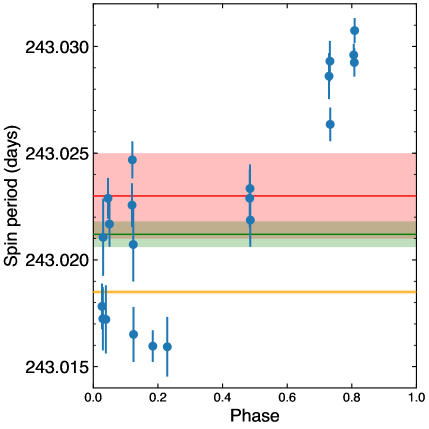
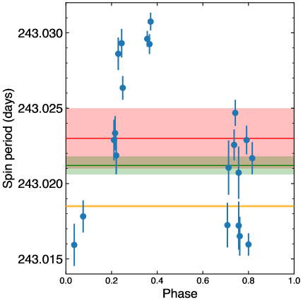
Supplementary Figure 6: Instantaneous spin period measurements of Venus folded onto candidate periodicities at (Top left) 4996.4 days, (Top right) 315.5 days, (Bottom left) 1067.9 days, and (Bottom right) 202.4 days. The origin of phase is 2000 FEB 22 10:43:58 TDB.

7 Identification of candidate periodicities related to spin, orbital, and diurnal frequencies

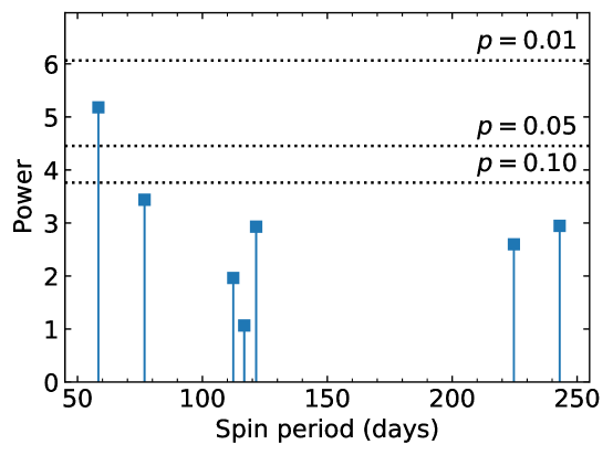
Supplementary Figure 7: Lomb periodogram analysis of periodicities related to the to the spin ($\omega$), orbital ($n$), and diurnal ($\omega+n$) frequencies. The horizontal dashed lines show the false alarm probabilities or significance levels. Only the semidiurnal period at 58.4 days reaches a $p=0.05$ level of significance by this metric.

$P$ (days)	Power	$p$-value	Frequency
243.023	2.9454	2.26e-01	$\omega$
224.701	2.5981	3.20e-01	$n$
121.511	2.9294	2.30e-01	$2\omega$
116.752	1.0657	1.48e+00	$\omega+n$
112.350	1.9627	6.04e-01	$2n$
76.831	3.4380	1.38e-01	$\omega+2n$
58.376	5.1808	2.42e-02	$2\omega+2n$

Supplementary Table 5: Lomb periodogram analysis of periodicities in Venus LOD variations, with trial periods associated with spin ($\omega$), orbital ($n$), and diurnal ($\omega+n$) frequencies. Columns show trial period, power, the probability of false alarm or significance level, and frequency.

$P$ (days)	$\theta_{\rm PDM}$	$p$-value	Frequency
243.023	0.5811	8.70e-02	$\omega$
224.701	0.2722	1.50e-03	$n$
121.511	0.6714	2.07e-01	$2\omega$
116.752	0.1856	5.00e-04	$\omega+n$
112.350	0.4430	4.00e-02	$2n$
76.831	0.6204	3.04e-01	$\omega+2n$
58.376	0.1842	4.20e-02	$2\omega+2n$

Supplementary Table 6: Results of PDM analysis of Venus LOD variations, with trial periods associated with spin ($\omega$), orbital ($n$), and diurnal ($\omega+n$) frequencies. Columns show trial period, PDM statistic $\theta$, a pseudo $p$-value obtained by ranking 2000 Monte Carlo trials where the observed spin periods are permuted prior to PDM analysis, and frequency. The semidiurnal period ranks first, but only marginally so compared to the diurnal period. The orbital period is a distant third.

References

- [1] Smrekar, S. E., Davaille, A. & Sotin, C. Venus Interior Structure and Dynamics. Space Sci. Rev. 214, 88 (2018).
- [2] Dumoulin, C., Tobie, G., Verhoeven, O., Rosenblatt, P. & Rambaux, N. Tidal constraints on the interior of Venus. J. Geophys. Res. Planets 122, 1338–1352 (2017).
- [3] O’Rourke, J. G., Gillmann, C. & Tackley, P. Prospects for an ancient dynamo and modern crustal remanent magnetism on Venus. Earth Planet. Sci. Lett. 502, 46–56 (2018).
- [4] Davies, M. E. et al. The rotation period, direction of the north pole, and geodetic control network of Venus. J. Geophys. Res. 97, 13141– (1992).
- [5] Mueller, N. T., Helbert, J., Erard, S., Piccioni, G. & Drossart, P. Rotation period of Venus estimated from Venus Express VIRTIS images and Magellan altimetry. Icarus 217, 474–483 (2012).
- [6] Campbell, B. A. et al. The mean rotation rate of Venus from 29 years of Earth-based radar observations. Icarus 332, 19–23 (2019).
- [7] Yoder, C. F. Venusian Spin Dynamics. In Venus II: Geology, Geophysics, Atmosphere, and Solar Wind Environment, 1087– (U. of Az. Press, 1997).
- [8] Sánchez-Lavega, A., Lebonnois, S., Imamura, T., Read, P. & Luz, D. The Atmospheric Dynamics of Venus. Space Sci. Rev. 212, 1541–1616 (2017).
- [9] Horinouchi, T. et al. How waves and turbulence maintain the super-rotation of Venus’ atmosphere. Science 368, 405–409 (2020).
- [10] Venus Exploration Assessment Group. Roadmap for Venus Exploration (2019).
- [11] Kaula, W. M. An Introduction to Planetary Physics: The Terrestrial Planets (Wiley, 1968).
- [12] Williams, J. G. Contributions to the Earth’s obliquity rate, precession, and nutation. Astron. J. 108, 711–724 (1994).
- [13] Folkner, W. M., Yoder, C. F., Yuan, D. N., Standish, E. M. & Preston, R. A. Interior structure and seasonal mass redistribution of Mars from Radio Tracking of Mars Pathfinder. Science 278, 1749–1751 (1997).
- [14] Standish, E. M. & Williams, J. G. Orbital ephemerides of the sun, moon, and planets. In Urban, S. E. & Seidelmann, P. K. (eds.) Explanatory Supplement to the Astronomical Almanac (University Science Books, 2013).
- [15] Konopliv, A. S., Banerdt, W. B. & Sjogren, W. L. Venus Gravity: 180th Degree and Order Model. Icarus 139, 3–18 (1999).
- [16] Cottereau, L. & Souchay, J. Rotation of rigid Venus: a complete precession-nutation model. Astron. Astrophys. 507, 1635–1648 (2009).
- [17] Saunders, R. S. et al. Magellan mission summary. J. Geophys. Res. 97, 13067–13090 (1992).
- [18] Shapiro, I. I., Campbell, D. B. & de Campli, W. M. Nonresonance rotation of Venus. Astrophys. J. Lett. 230, L123–L126 (1979).
- [19] Zohar, S., Goldstein, R. M. & Rumsey, H. C. A new radar determination of the spin vector of Venus. Astronomical Journal 85, 1103–1111 (1980).
- [20] Shapiro, I. I., Chandler, J. F., Campbell, D. B., Hine, A. A. & Stacy, N. J. S. The spin vector of Venus. Astron. J. 100, 1363–1368 (1990).
- [21] Slade, M. A., Zohar, S. & Jurgens, R. F. Venus - Improved spin vector from Goldstone radar observations. Astron. J. 100, 1369–1374 (1990).
- [22] Goldreich, P. & Peale, S. Spin-orbit coupling in the solar system. Astron. J. 71, 425– (1966).
- [23] Goldreich, P. & Peale, S. Spin-orbit coupling in the solar system. II. The resonant rotation of Venus. Astron. J. 72, 662– (1967).
- [24] Gold, T. & Soter, S. Atmospheric Tides and the Resonant Rotation of Venus. Icarus 11, 356– (1969).
- [25] Ingersoll, A. P. & Dobrovolskis, A. R. Venus’ rotation and atmospheric tides. Nature 275, 37– (1978).
- [26] Dobrovolskis, A. R. & Ingersoll, A. P. Atmospheric tides and the rotation of Venus. I - Tidal theory and the balance of torques. Icarus 41, 1–17 (1980).
- [27] Correia, A. C. M. & Laskar, J. The four final rotation states of Venus. Nature 411, 767–770 (2001).
- [28] Bills, B. G. Variations in the rotation rate of Venus due to orbital eccentricity modulation of solar tidal torques. J. Geophys. Res. 110, 11007– (2005).
- [29] Hide, R., Birch, N. T., Morrison, L. V., Shea, D. J. & White, A. A. Atmospheric Angular Momentum Fluctuations and Changes in the Length of the Day. Nature 286, 114– (1980).
- [30] Lebonnois, S. et al. Superrotation of Venus’ atmosphere analyzed with a full general circulation model. J. Geophys. Res. Planets 115, E06006 (2010).
- [31] Cottereau, L., Rambaux, N., Lebonnois, S. & Souchay, J. The various contributions in Venus rotation rate and LOD. Astron. Astrophys. 531, A45 (2011).
- [32] Parish, H. F. et al. Decadal variations in a Venus general circulation model. Icarus 212, 42–65 (2011).
- [33] Margot, J. L. A data-taking system for planetary radar applications. J. Astron. Instrum. 10 (2021).
- [34] Margot, J. L., Peale, S. J., Jurgens, R. F., Slade, M. A. & Holin, I. V. Large Longitude Libration of Mercury Reveals a Molten Core. Science 316, 710–714 (2007).
- [35] Margot, J. L. et al. Mercury’s moment of inertia from spin and gravity data. J. Geophys. Res. Planets 117 (2012).
- [36] Stark, A. et al. First MESSENGER orbital observations of Mercury’s librations. Geophys. Res. Lett. 42, 7881–7889 (2015).
- [37] Bendat, J. S. & Piersol, A. G. Random Data. Analysis and Measurement Procedures (Wiley, 1986), 2nd, revised and expanded edn.
- [38] Correia, A. C. M., Laskar, J. & de Surgy, O. N. Long-term evolution of the spin of Venus I. theory. Icarus 163, 1–23 (2003).
- [39] Correia, A. C. M. & Laskar, J. Long-term evolution of the spin of Venus II. numerical simulations. Icarus 163, 24–45 (2003).
- [40] Gross, R. Earth Rotation Variations – Long Period. In Schubert, G. (ed.) Treatise on Geophysics, 239 – 294 (Elsevier, Amsterdam, 2007).
- [41] Goldreich, P. & Peale, S. J. Resonant Rotation for Venus? Nature 209, 1117–1118 (1966).
- [42] Navarro, T., Schubert, G. & Lebonnois, S. Atmospheric mountain wave generation on Venus and its influence on the solid planet’s rotation rate. Nat. Geosci. 11, 487–491 (2018).
- [43] Fukuhara, T. et al. Large stationary gravity wave in the atmosphere of Venus. Nat. Geosci. 10, 85–88 (2017).
- [44] Kouyama, T. et al. Topographical and Local Time Dependence of Large Stationary Gravity Waves Observed at the Cloud Top of Venus. Geophys. Res. Lett. 44, 12,098–12,105 (2017).
- [45] Mitchell, J. L. Coupling Convectively Driven Atmospheric Circulation to Surface Rotation: Evidence for Active Methane Weather in the Observed Spin Rate Drift of Titan. Astrophys. J. 692, 168–173 (2009).
- [46] Green, P. E. Radar Astronomy Measurement Techniques. Tech. Rep. 282, MIT Lincoln Laboratory (1962).
- [47] Green, P. E. Radar astronomy. chap. Radar Measurements (McGraw-Hill, 1968).
- [48] Kholin (Holin), I. V. Spatial-temporal coherence of a signal diffusely scattered by an arbitrarily moving surface for the case of monochromatic illumination. Radiophys. Quant. Elec. 31, 371–374 (1988). Translated from I. V. Holin, Izvestiya Vysshikh Uchebnykh Zavedenii, Radiofizika, 31, pp. 515-518.
- [49] Kholin (Holin), I. V. Accuracy of body-rotation-parameter measurement with monochromatic illumination and two-element reception. Radiophys. Quant. Elec. 35, 284–287 (1992). Translated from I. V. Holin, Izvestiya Vysshikh Uchebnykh Zavedenii, Radiofizika, 35, pp. 433-439.
- [50] Margot, J. L., Hauck, S. A., Mazarico, E., Padovan, S. & Peale, S. J. Mercury’s Internal Structure. In Solomon, S. C., Nittler, L. R. & Anderson, B. J. (eds.) Mercury: The View after MESSENGER, 85–113 (Cambridge University Press, 2018).
- [51] Duan, X., Moghaddam, M., Wenkert, D., Jordan, R. L. & Smrekar, S. E. X band model of venus atmosphere permittivity. Radio Science 45 (2010).
- [52] Dziewonski, A. M. & Anderson, D. L. Preliminary reference earth model. Phys. Earth Planet. Inter. 25, 297–356 (1981).
- [53] Press, W. H., Teukolsky, S. A., Vetterling, W. T. & Flannery, B. P. Numerical Recipes in C (Cambridge University Press, Cambridge, USA, 1992), 2nd edn.
- [54] Williams, P. K. G., Clavel, M., Newton, E. & Ryzhkov, D. pwkit: Astronomical utilities in Python (2017). 1704.001.
- [55] Archinal, B. A. et al. Report of the IAU Working Group on Cartographic Coordinates and Rotational Elements: 2015. Celestial Mechanics and Dynamical Astronomy 130, 22 (2018).
- [56] Kelly, B. C., Becker, A. C., Sobolewska, M., Siemiginowska, A. & Uttley, P. Flexible and Scalable Methods for Quantifying Stochastic Variability in the Era of Massive Time-domain Astronomical Data Sets. Astrophys. J. 788, 33 (2014).
Acknowledgments
This article is dedicated to the memory of Raymond F. Jurgens, who was instrumental in acquiring the data for this work. We thank M. A. Slade, J. T. Lazio, T. Minter, K. O’Neil, and F. J. Lockman for assistance with scheduling the observations. We thank B. A. Archinal, P. M. Davis, S. Lebonnois, J. L. Mitchell, and C. F. Wilson for useful comments and A. Lam for assistance with Figure 1. The Green Bank Observatory is a facility of the National Science Foundation operated under cooperative agreement by Associated Universities, Inc. Part of this work was supported by the Jet Propulsion Laboratory, operated by Caltech under contract with NASA. We are grateful for NASA’s Navigation and Ancillary Information Facility software and data kernels, which greatly facilitated this research. JLM was funded in part by NASA grants NNG05GG18G, NNX09AQ69G, NNX12AG34G, 80NSSC19K0870.