Direct measurement of ultrafast temporal wavefunctions

Abstract

The large capacity and robustness of information encoding in the temporal mode of photons is important in quantum information processing, in which characterizing temporal quantum states with high usability and time resolution is essential. We propose and demonstrate a direct measurement method of temporal complex wavefunctions for weak light at a single-photon level with subpicosecond time resolution. Our direct measurement is realized by ultrafast metrology of the interference between the light under test and self-generated monochromatic reference light; no external reference light or complicated post-processing algorithms are required. Hence, this method is versatile and potentially widely applicable for temporal state characterization.

I Introduction

The temporal–spectral mode of photons offers an attractive platform for quantum information processing in terms of a large capacity due to its high dimensionality and robustness in fiber and waveguide transmission. To date, many applications using the temporal–spectral mode have been proposed and realized in quantum information processing fields such as quantum computation, quantum cryptography, and quantum metrology Humphreys et al. (2014); Nunn et al. (2013); Mower et al. (2013); Lukens et al. (2014); Roslund et al. (2014); Brecht et al. (2015); Lamine et al. (2008); Jian et al. (2012); Humphreys et al. (2013); Ryczkowski et al. (2016). In these applications, the full characterization of quantum states, i.e., complex wavefunctions, is crucial for developing reliable quantum operations. In addition, temporal-mode characterization for high-speed and precise processing often requires ultrafast time resolution, such as on the subpicosecond scale.

Several established methods, such as frequency-resolved optical gating (FROG) and spectral phase interferometry for direct electric field reconstruction (SPIDER), are well known for measuring the temporal–spectral mode of classical light Walmsley and Dorrer (2009). These methods, however, utilize the nonlinear optical processes of the light under test, which are difficult to observe for weak light at the single-photon level. In recent years, various methods for characterizing the temporal–spectral mode of quantum light have been demonstrated, such as single photons and entangled photon pairs Ansari et al. (2018); Polycarpou et al. (2012); Qin et al. (2015); Yang et al. (2018); Wasilewski et al. (2007); Xu et al. (2019); Chen et al. (2015); Davis et al. (2018a, 2020, b); MacLean et al. (2019); Thiel et al. (2020), and some have achieved ultrafast (subpicosecond) time resolution Ansari et al. (2018); Polycarpou et al. (2012); Wasilewski et al. (2007); Davis et al. (2018a, 2020, b); MacLean et al. (2019); Thiel et al. (2020). While these methods differ in the details of their measurement procedures, they have a common procedure to reconstruct the form of the wavefunction: projective measurements for the entire temporal (or spectral or other basis) wavefunction have to be performed first, and then the measurement data is post-processed, as shown in Fig. 1(a). In other words, even for acquiring only one part of the wavefunction, measurement of the entire wavefunction is essential. Each set of measurement data before post-processing contains partial information of the wavefunction but is not itself the wavefunction.

As a more suitable measurement method for the form of the wavefunction, direct measurement Lundeen et al. (2011) is the focus of this study. The direct measurement of a wavefunction $\psi(t)$ is defined as the measurement that can reconstruct the complex value $\psi(t_{0})$ only using the measurement data at the point $t=t_{0}$, as shown in Fig. 1(b); that is, the measurement data at $t_{0}$ directly correspond to the complex value $\psi(t_{0})$. Direct measurement was first demonstrated for the transverse spatial wavefunction of single photons Lundeen et al. (2011) using a technique called weak measurement Aharonov et al. (1988), and then for wavefunctions and density matrices in various degrees of freedom Lundeen and Bamber (2012); Malik et al. (2014); Salvail et al. (2013); Shi et al. (2015); Thekkadath et al. (2016). While direct measurement was introduced to give the operational meaning of the complex-valued wavefunction, it also provides a practical advantage of requiring only one measurement basis. Although direct measurement using weak measurement has drawbacks in its approximation error and low efficiency due to the nature of weak measurement, in recent years it has been reported that direct measurement can also be realized using strong (projection) measurement both theoretically Zou et al. (2015); Vallone and Dequal (2016); Ogawa et al. (2019) and experimentally Denkmayr et al. (2017); Calderaro et al. (2018). Therefore, applying direct measurement using strong measurement to the temporal wavefunction of photons can provide a practical characterization method for temporal wavefunctions, which avoids the requirement of post-processing the measurement data of the entire wavefunction.

In this paper, we propose a direct measurement method of temporal complex wavefunctions that can be performed for weak light at a single-photon level with subpicosecond time resolution. Our direct measurement is realized by ultrafast metrology (time gate measurement) of the interference between the light under test and the self-generated monochromatic reference light with several phase differences. This mechanism is simple compared to other measurement methods of the temporal–spectral mode of quantum light; that is, it does not require external reference light or complicated post-processing of the measurement data. We also experimentally demonstrate this direct measurement method of the temporal wavefunction of light at a single-photon level and examine the validity of the measurement results.

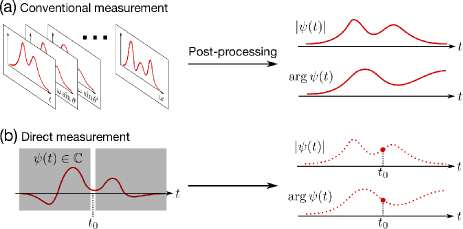
Figure 1: Comparison of the concepts of the conventional and direct measurement methods. (a) In conventional measurement methods, measurements of the entire wavefunction are usually performed first, and then the measurement data are post-processed to reconstruct the entire wavefunction. (b) In the direct measurement method, the measurement data at the time $t_{0}$ directly correspond to the complex value $\psi(t_{0})$ of the wavefunction $\psi(t)$ at $t_{0}$.

II Theory

The proposed method for direct measurement of the temporal wavefunction is based on our previous study Ogawa et al. (2019). The wavefunction under test $\psi(t)$ is the temporal representation of the pulse-mode state $|\psi\rangle$, and its spectral representation $\tilde{\psi}(\omega)$ is given by the Fourier transform of $\psi(t)$. $\psi(t)$ can be represented by the product of the complex-valued envelope function $\psi_{\mathrm{env}}(t)$ and the carrier term ${\mathrm{e}}^{-{\mathrm{i}}\omega_{0}t}$ as $\psi(t)=\psi_{\mathrm{env}}(t){\mathrm{e}}^{-{\mathrm{i}}\omega_{0}t}$, where $\omega_{0}$ is the reference carrier frequency. We assume that $\omega_{0}$ is known and then consider measuring $\psi_{\mathrm{env}}(t)$ instead of $\psi(t)$. The Fourier transform of $\psi_{\mathrm{env}}(t)$, $\tilde{\psi}_{\mathrm{env}}(\omega)$, satisfies the relation $\tilde{\psi}_{\mathrm{env}}(\omega)=\tilde{\psi}(\omega+\omega_{0})$.

The basic mechanism common to most direct measurements Lundeen et al. (2011); Lundeen and Bamber (2012); Malik et al. (2014); Salvail et al. (2013); Shi et al. (2015); Thekkadath et al. (2016); Zou et al. (2015); Vallone and Dequal (2016); Ogawa et al. (2019); Denkmayr et al. (2017); Calderaro et al. (2018); Ogawa et al. (2019) is the interference between the signal wavefunction under test $\psi(t)=\psi_{\mathrm{env}}(t){\mathrm{e}}^{-{\mathrm{i}}\omega_{0}t}$ and a self-generated uniform reference wave $\psi_{0}{\mathrm{e}}^{-{\mathrm{i}}\omega_{0}t}$ with four phase differences $0$, $\pi/2$, $\pi$, and $3\pi/2$. The probability that their superposition state is projected onto time $t$ and phase difference $\theta$ is given by $P(t,\theta)=|\psi(t)+{\mathrm{e}}^{-{\mathrm{i}}(\omega_{0}t+\theta)}\psi_{0}|^{2}=|\psi_{\mathrm{env}}(t)+{\mathrm{e}}^{-{\mathrm{i}}\theta}\psi_{0}|^{2}$. The differences between $P(t,0)$ and $P(t,\pi)$ and between $P(t,\pi/2)$ and $P(t,3\pi/2)$ give the real and imaginary parts of $\psi_{\mathrm{env}}(t)$, respectively:

$$P(t,0)-P(t,\pi) \propto\mathrm{Re}[\psi_{\mathrm{env}}(t)],$$ (1)

$$P(t,\pi/2)-P(t,3\pi/2) \propto\mathrm{Im}[\psi_{\mathrm{env}}(t)].$$ (2)

Their proportional coefficients are equal and can be determined by the normalization condition of the wavefunction.

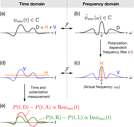
Figure 2: Procedure of direct measurement of the temporal wavefunction. (a), (b) Temporal and spectral representations of the pulse-mode state $|\psi\rangle$, respectively. Its polarization mode is set to the diagonal state $|\mathrm{D}\rangle$. (c) Wavefunction after applying the polarization-dependent frequency filter at $\omega=0$ (the actual frequency is $\omega_{0}$) to the wavefunction of (b). Only the frequency $\omega=0$ component remains for the horizontally polarized light. (d) Temporal representation of the wavefunction of (c). The horizontally polarized component has an almost uniform distribution, which serves as a reference for the magnitude and phase of the vertically polarized temporal wavefunction $\psi_{\mathrm{env}}(t)$. (e) Real and imaginary parts of $\psi_{\mathrm{env}}(t)$, which are reconstructed by combining the projection probability distributions $P(t,\mathrm{D})$, $P(t,\mathrm{A})$, $P(t,\mathrm{R})$, and $P(t,\mathrm{L})$ of time and polarization measurement for the wavefunction of (d).

To realize the above mechanism, our direct measurement method Ogawa et al. (2019) uses a qubit (two-state quantum system) probe mode to prepare the four phase differences; we utilize the polarization mode of the photons spanned by the horizontal and vertical states $|\mathrm{H}\rangle$ and $|\mathrm{V}\rangle$. We define the four polarization states as follows: diagonal $|\mathrm{D}\rangle:=(|\mathrm{H}\rangle+|\mathrm{V}\rangle)/\sqrt{2}$, anti-diagonal $|\mathrm{A}\rangle:=(|\mathrm{H}\rangle-|\mathrm{V}\rangle)/\sqrt{2}$, right-circular $|\mathrm{R}\rangle:=(|\mathrm{H}\rangle+{\mathrm{i}}|\mathrm{V}\rangle)/\sqrt{2}$, and left-circular $|\mathrm{L}\rangle:=(|\mathrm{H}\rangle-{\mathrm{i}}|\mathrm{V}\rangle)/\sqrt{2}$. The procedure of our direct measurement of the temporal wavefunction is shown in Fig. 2. Let the initial state be $|\varPsi_{0}\rangle:=|\psi\rangle|\mathrm{D}\rangle=|\psi\rangle(|\mathrm{H}\rangle+|\mathrm{V}\rangle)/\sqrt{2}$. The temporal and spectral representations of $|\varPsi_{0}\rangle$ are shown in Figs. 2(a) and (b), respectively. First, we extract the frequency $\omega=0$ component (the actual frequency is $\omega_{0}$) from the horizontally polarized light using a polarization-dependent frequency filter. This operation is ideally described by the projection operator $|\omega_{0}\rangle\langle\omega_{0}|\otimes|\mathrm{H}\rangle\langle\mathrm{H}|+\hat{1}\otimes|\mathrm{V}\rangle\langle\mathrm{V}|$, and the unnormalized state after the projection is given by $|\varPsi_{1}\rangle:=(|\omega_{0}\rangle\langle\omega_{0}|\psi\rangle|\mathrm{H}\rangle+|\psi\rangle|\mathrm{V}\rangle)/\sqrt{2}$. Second, we perform projection measurements of time and polarization for $|\varPsi_{1}\rangle$. The projections onto D, A, R, L polarizations correspond to the preparations of the four phase differences $0$, $\pi$, $\pi/2$, and $3\pi/2$, respectively. The projection operator onto time $t$ and polarization $\phi$ is described as $|t\rangle\langle t|\otimes|\phi\rangle\langle\phi|$, and its projection probability is given by $P(t,\phi)=\langle\varPsi_{1}|(|t\rangle\langle t|\otimes|\phi\rangle\langle\phi|)|\varPsi_{1}\rangle/\langle\varPsi_{1}|\varPsi_{1}\rangle$. Using $P(t,\phi)$ for $\phi=\mathrm{D}$, $\mathrm{A}$, $\mathrm{R}$, and $\mathrm{L}$, the real and imaginary parts of $\psi_{\mathrm{env}}(t)$ are obtained as

$$P(t,\mathrm{D})-P(t,\mathrm{A}) \propto\mathrm{Re}[\langle\psi|\omega_{0}\rangle\langle\omega_{0}|t\rangle\langle t|\psi\rangle]{}$$

$$\propto\mathrm{Re}[{\mathrm{e}}^{{\mathrm{i}}\omega_{0}t}\psi(t)]=\mathrm{Re}[\psi_{\mathrm{env}}(t)],$$ (3)

$$P(t,\mathrm{R})-P(t,\mathrm{L}) \propto\mathrm{Im}[\psi_{\mathrm{env}}(t)],$$ (4)

where $\langle\psi|\omega_{0}\rangle$ is a constant that does not depend on $t$ and $\langle\omega_{0}|t\rangle={\mathrm{e}}^{{\mathrm{i}}\omega_{0}t}/\sqrt{2\pi}$.

Here, we emphasize the following two points. First, our measurement method satisfies the definition of direct measurement mentioned previously. Indeed, to obtain the complex value of $\psi_{\mathrm{env}}(t_{0})$, this measurement method requires only the four projection probabilities $P(t_{0},\phi)$ ($\phi=\mathrm{D},\mathrm{A},\mathrm{R},\mathrm{L}$) at time $t_{0}$. Second, our direct measurement method is more accurate and efficient than conventional direct measurement methods using weak measurement Lundeen et al. (2011); Lundeen and Bamber (2012); Malik et al. (2014); Salvail et al. (2013); Shi et al. (2015); Thekkadath et al. (2016). Our measurement method causes interference between the signal and the self-generated uniform reference wave using the polarization-dependent frequency filter (projection measurement) instead of weak measurement. Therefore, our method can avoid the approximation error and low measurement efficiency associated with weak measurement. We note that the polarization degree of freedom, which is used to provide the four phase differences in the interference, can be replaced by another degree of freedom such as path mode when the polarization mode is already used or unstable for use.

III Experiments

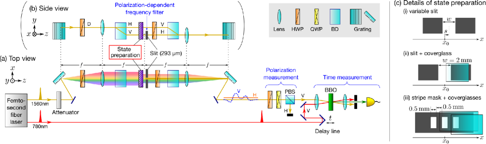
Figure 3: Experimental setup. (a) Top view of the whole system. (b) Side view of the 4-$f$ system. HWP: half-wave plate, QWP: quarter-wave plate, BD: beam displacer, PBS: polarizing beam splitter, BBO: $\upbeta$-BaB₂O₄ crystal. (c) Details of state preparation. (i) Variable slit ($w$: gap width, $s$: displacement of the gap center from $x_{0}$, $x_{0}$: center position of the slit for polarization-dependent frequency filtering). (ii) Slit ($w=2\,\mathrm{mm}$, $s=0\,\mathrm{mm}$) and coverglass ($170\pm 5\,\mathrm{mm}$ thickness). (iii) Stripe mask (0.5 mm gap) and two coverglasses.

We demonstrate the direct measurement of the temporal wavefunction using the measurement system shown in Fig. 3. The femtosecond fiber laser (Menlo Systems C-Fiber 780) emits two pulsed light beams with central wavelengths 1560 nm and 780 nm in synchronization (repetition rate 100 MHz). The 1560 nm beam is used as the signal under test, and the 780 nm beam [76.5 mW, 79.2 fs full width at half maximum (FWHM)] as the gate pulse for the time gate measurement . We prepare the signal power in the following two conditions using the attenuator: the classical-light (CL) condition, in which the average photon number is 366 photons/pulse ($4.69\,\mathrm{nW}$); and the single-photon-level (SPL) condition, in which the average photon number is 0.58 photons/pulse ($7.47\,\mathrm{pW}$) and the probability of one or fewer photons per pulse is 0.885. The SPL condition is used to demonstrate that our direct measurement system works even for a signal as weak as a single-photon level.

The 1560 nm beam then enters the 4-$f$ system composed of the gratings (600 grooves/mm) and lenses (focal length $f=300\,\mathrm{mm}$). At the center of the 4-$f$ system, the spectral distribution is mapped onto the transverse spatial distribution, where state preparation followed by polarization-dependent frequency filtering is performed. As seen in Fig. 3(b), two beam displacers (BDs) are set in the 4-$f$ system to divide the optical path according to the polarization; the polarization-dependent frequency filter is realized by inserting a slit (293 $\upmu$m width) in one of the paths. In contrast, the state preparation before the slit is performed equally for the two beams. After the state preparation followed by polarization-dependent frequency filtering, the polarizations of the two beams are exchanged by the half-wave plate (HWP) and then combined by the second BD so that the two optical path lengths are equal.

In the state preparation, we prepare the three types of states shown in Fig. 3(c). A variable slit with gap width $w$ and displacement $s$ is used to quantitatively evaluate the measured temporal wavefunction. The coverglass is used to cause a phase change. As the magnitude of the phase change depends sensitively on the inclination of the coverglass, we assume that this magnitude is unknown. The combination of the stripe mask and coverglasses is used to demonstrate the direct measurement of a complicated wavefunction.

After the 4-$f$ system, the beam is projected onto one of the D, A, R, or L polarizations by the HWP, quarter-wave plate, and polarizing beam splitter. Subsequently, the beam is projected onto time $t$ by the time gate measurement, which is realized by sum-frequency generation (SFG) of the signal beam and the 780 nm gate pulse with delay $t$. In SFG, these two beams are focused on the $\upbeta$-BaB₂O₄ crystal by the lens ($f=50\,\mathrm{mm}$), and their sum-frequency light (520 nm wavelength) is emitted at an intensity proportional to the product of the two input temporal intensities. By scanning the delay of the gate pulse $t$, sum-frequency light with an intensity proportional to the time intensity distribution of the signal light is extracted. Finally, the sum-frequency light is spatially and spectrally filtered to remove the stray light (not shown in the figure) and then detected by a single-photon counting module (Laser Components COUNT-NIR).

For comparison, we additionally perform intensity (projection) measurements in time and frequency for the state under test in the CL condition. The state under test is extracted by the projection measurement onto V polarization from the output light of the 4-$f$ system. The intensity measurements in time and frequency are realized by the time gate measurement and using an optical spectrum analyzer (Advantest Q8384), respectively. The obtained temporal and spectral intensity distributions are used to examine the validity of the direct measurement results.

We note that the spectral width $\delta\omega$ extracted by the polarization-dependent frequency filter (1.08 THz FWHM) is not sufficiently small compared to those of the states under test generated by the slit or the stripe mask ($\sim 6\,\mathrm{THz}$). In this condition, the spectral wavefunction after the frequency filter should be approximated by the rectangle function $\mathrm{rect(\omega/\delta\omega)}$, which is zero outside the interval $[-\delta\omega/2,\delta\omega/2]$ and unity inside it. In this case, the right sides of Eqs. (3) and (4) are replaced by $\mathrm{sinc}(\delta\omega t/2)\mathrm{Re}[\psi_{\mathrm{env}}(t)]$ and $\mathrm{sinc}(\delta\omega t/2)\mathrm{Im}[\psi_{\mathrm{env}}(t)]$, respectively, where $\mathrm{sinc}(x):=\sin(x)/x$. To obtain $\mathrm{Re}[\psi_{\mathrm{env}}(t)]$ and $\mathrm{Im}[\psi_{\mathrm{env}}(t)]$, we make a correction by dividing the measured wavefunctions by $\mathrm{sinc}(\delta\omega t/2)$, which is independent of $\psi_{\mathrm{env}}(t)$ and was determined by prior measurement. On the other hand, the time width of the gate pulses (79.2 fs FWHM) is considered to be sufficiently smaller than those of the states under test ($\sim 3\,\mathrm{ps}$). Hence, we assume here that the effect of the width of the time measurement can be ignored. The detailed calculation accounting for both the effects of the finite frequency and the time widths is given in Appendix A.

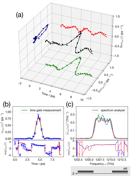
Figure 4: Results of the direct measurement of the wavefunction generated by the variable slit ($w=2.0$ mm, $s=0.0$ mm). (a) 3D plot of the measured temporal wavefunction (black line and dots). The red, green, and navy lines and dots are its projections on the real, imaginary, and amplitude phase planes, respectively. The solid lines and the dots are the measurement results in the CL and SPL conditions, respectively. In the SPL condition, photon counting was performed for 25 s per measurement point. The error bars are omitted here. (b) Intensity (upper panel) and phase distribution (lower panel) calculated from the measured temporal wavefunction. The red solid line and blue dots are the measurement results in the CL and SPL conditions, respectively. The error bars were calculated from the square root of the counted photon number (shot noise). The green dotted line in the upper panel is the temporal intensity distribution obtained by the time gate measurement of the wavefunction under test. (c) Intensity (upper panel) and phase distribution (lower panel) of the spectral wavefunction obtained by Fourier-transforming the measured temporal wavefunction. The red solid line and blue dashed line are the distributions in the CL and SPL conditions, respectively. The green dotted line in the upper panel is the spectral intensity distribution obtained using the optical spectrum analyzer for the wavefunction under test.

In the following, we show the experimental results for state preparations (i)–(iii) in Fig. 3(c) in order. First, the spectral wavefunction generated by the variable slit with gap width $w$ and displacement $s$ is given by a rectangle function $\mathrm{rect}[(\omega-\omega_{\mathrm{c}})/\Delta\omega]$. The spectral width $\Delta\omega$ and central frequency $\omega_{\mathrm{c}}$ are expressed as $\Delta\omega=\alpha w$ and $\omega_{\mathrm{c}}=\alpha s$, respectively, where the proportional constant $\alpha:=2.41\,\mathrm{THz/mm}$ is derived from the geometrical configuration of our 4-$f$ system. The temporal wavefunction obtained by Fourier-transforming $\mathrm{rect}[(\omega-\omega_{\mathrm{c}})/\Delta\omega]$ is ${\mathrm{e}}^{{\mathrm{i}}\omega_{\mathrm{c}}t}\mathrm{sinc}(\Delta\omega t/2)$, and the time width $\Delta t$ between the two central zeros of this sinc function and the phase gradient $\kappa$ are given by $\Delta t=4\pi/\Delta\omega=4\pi/(\alpha w)$ and $\kappa=\omega_{\mathrm{c}}=\alpha s$, respectively. Therefore, in this state preparation, the form of the temporal wavefunction can be controlled quantitatively by changing $w$ and $s$.

We display the 3D plot of the result of the direct measurement of the temporal wavefunction generated by the variable slit ($w=2.0$ mm, $s=0.0$ mm) in Fig. 4(a). There is no significant difference between the measurement results under the CL condition (lines) and those under the SPL condition (dots), while some fluctuation due to the shot noise is observed in the results in the SPL condition. The intensity (square of the amplitude) and phase distributions of the measured temporal wavefunction are shown in Fig. 4(b), and those in the frequency domain, obtained by Fourier-transforming the measured temporal wavefunction, are shown in Fig. 4(c). Furthermore, the temporal and spectral intensity distributions obtained by the time gate measurement and optical spectrum analyzer are displayed as green dotted lines in Figs. 4(b) and (c), respectively. The agreement of these intensity measurement distributions with the intensity distribution reconstructed from the directly measured wavefunction supports the validity of our direct measurement results. A quantitative comparison between them using classical fidelity is discussed at the end of this section.

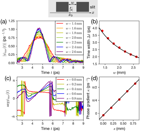
Figure 5: Results of the direct measurement when the gap width $w$ and displacement of the gap center $s$ of the variable slit are changed. (a) Measurement results of the magnitude of the temporal wavefunction when $w$ is changed from 1.4 mm to 2.6 mm while $s$ is fixed at $s=0\,\mathrm{mm}$. (b) Relationship between $w$ and time width $\Delta t$ obtained from the measured curves. The solid black line represents the theoretical curve $\Delta t=4\pi/(\alpha w)$. (c) Measurement results of the phase of the temporal wavefunction when $s$ is changed from 0.0 mm to 0.8 mm while $w$ is fixed at $w=2.0\,\mathrm{mm}$. (d) Relationship between $s$ and phase gradient $\kappa$ obtained from the measured curves. The solid black line represents the theoretical curve $\kappa=\alpha s+\kappa_{0}$.

Next, we examine the change in the measured temporal wavefunction when the gap width $w$ and displacement $s$ of the variable slit are changed. All these measurements are performed in the CL condition. Figure 5(a) shows the direct measurement results of the magnitude of the temporal wavefunction when $w$ is changed from 1.4 mm to 2.6 mm while $s$ is fixed at $s=0\,\mathrm{mm}$. The time widths $\Delta t$ of the measured temporal amplitude, which are obtained by fitting the sinc function $A|\mathrm{sinc}[2\pi(t-t_{\mathrm{c}})/\Delta t]|$ to the measured curves, are plotted versus $w$ in Fig. 5(b). The values are in good agreement with the theoretical curve $\Delta t=4\pi/(\alpha w)$ (black line). Figure 5(c) shows the direct measurement results of the phase of the temporal wavefunction when $s$ is changed from 0.0 mm to 0.8 mm while $w$ is fixed as $w=2.0\,\mathrm{mm}$. The phase gradients $\kappa$ of the measured temporal phase, which are also obtained by fitting the linear function to the measured curves in the range of $t\in[3.75\,\mathrm{ps},5.75\,\mathrm{ps}]$, are plotted versus the displacement $s$ in Fig. 5(d). These values are also in good agreement with the theoretical curve $\kappa=\alpha s+\kappa_{0}$ (black line), where the offset value $\kappa_{0}:=-0.11\,\mathrm{ps}^{-1}$ is determined from the phase gradient when $s=0\,\mathrm{mm}$.

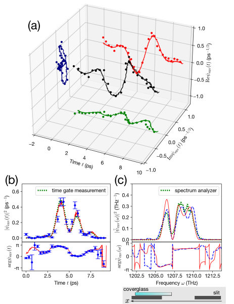
Figure 6: Results of the direct measurement of the temporal wavefunction generated by the slit ($w=2.0$ mm, $s=0.0$ mm) and coverglass. The notation of this figure is the same as in Fig. 4.

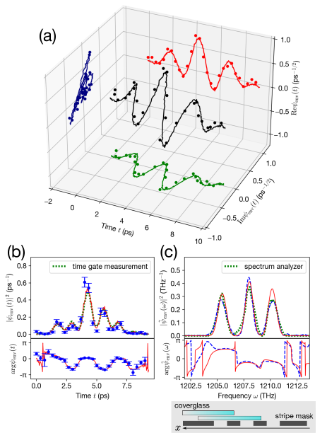
Figure 7: Results of the direct measurement of the temporal wavefunction generated by the stripe mask and coverglasses. The notation of this figure is the same as in Figs. 4 and 6.

We further demonstrate the direct measurement of the temporal wavefunction generated by the slit ($w=2.0$ mm, $s=0.0$ mm) with a coverglass and by the stripe mask with two coverglasses. The measurement results for the slit with a coverglass are shown in Figs. 6(a)–(c). It should be noted that the frequency wavefunction derived from the directly measured time wavefunction shows a stepwise phase change due to the phase added by the coverglass. The magnitude of the obtained phase step cannot be evaluated because its true value is not known in advance, as mentioned above. Nevertheless, the agreement of the spectral intensity distributions derived from the directly measured time wavefunction (red and blue lines) with the results of the frequency intensity measurement (green line) indicates that the characterization of the wavefunction by direct measurement is performed properly. Figures 7(a)–(c) show the measurement results for the stripe mask with two coverglasses, which have more complicated waveforms. In this case as well, the point to be noted is that the frequency wavefunction derived from the directly measured time wavefunction (red and blue lines) shows two stepwise phase changes as a result of the two coverglasses, and their intensity distributions are in agreement with the results of the frequency intensity measurement (green line). These results support the validity of the direct measurement method of the wavefunction.

Table 1: Classical fidelity (Bhattacharyya coefficient) between the intensity distributions calculated from the results of the direct measurement and those obtained by the projection measurements for panels (b) and (c) in Figs. 4, 6, and 7. CL and SPL indicate the signal power condition under which the direct measurements were performed.

	Time domain		Frequency domain
	[Panel (b)]		[Panel (c)]
	CL	SPL	CL	SPL
Fig. 4	0.999	0.993	0.995	0.990
Fig. 6	0.998	0.973	0.985	0.974
Fig. 7	0.999	0.976	0.987	0.970

Finally, we evaluate the closeness of the intensity distributions of the wavefunctions obtained by the direct measurement and those obtained by the intensity (projection) measurement using the classical fidelity (Bhattacharyya coefficient). The classical fidelity is defined as $\sum_{j}\sqrt{p_{j}q_{j}}$ for two probability distributions $\{p_{j}\}$ and $\{q_{j}\}$. Table 1 shows the classical fidelity between the intensity distributions obtained by the direct measurement and the projection measurements for panels (b) and (c) in Figs. 4, 6, and 7. We can see that these fidelities show high values close to 1.

IV Discussion

First, we describe the performance of the direct measurement system used in our experiment. The time resolution is determined by the time width of the gate pulse and the phase-matching bandwidth of SFG. In our case, the latter effect is negligible and the time resolution is 79.2 fs FWHM, which gives the subpicosecond resolution. On the other hand, the measurable range in the time domain is determined by the time width of the self-generated reference light in the shape of a sinc function. The time width between the two central zeros of the sinc function is 11.7 ps. Therefore, the dynamic range of our direct measurement system is evaluated to be $11.7\,\mathrm{ps}/79.2\,\mathrm{fs}=148$.

Next, we remark on previous studies related to direct measurement of the temporal wavefunction. A recently reported experiment on $\updelta$-quench measurement Zhang et al. (2019) has demonstrated measurement of the temporal mode of light by applying instantaneous phase modulation followed by projection onto a specific frequency. Although this method differs from direct measurement using weak measurement Lundeen et al. (2011) and our direct measurement method, it satisfies the definition of direct measurement of the temporal wavefunction. In this measurement, the time resolution did not reach the subpicosecond scale, and classical light much stronger than a single-photon level was used as the light under test.

In addition, a temporal-mode measurement method reported over 30 years ago Rothenberg and Grischkowsky (1987) also satisfies the definition of direct measurement. Although it was devised independently of the context of direct measurement, its configuration is similar to that of our direct measurement system. In this measurement, the time resolution reached the subpicosecond scale, while classical light was used as the light under test. As a characterization method of the temporal mode of classical light, this method is currently rarely used in contrast to other sophisticated methods such as FROG and SPIDER. However, the simple configuration of this method makes it suitable for the measurement of single photons, and the significance of our experiment is that it demonstrates this.

V Conclusion

We proposed a direct measurement method for characterizing the temporal wavefunction of single photons and experimentally demonstrated the direct measurement for several test wavefunctions. The experimental results showed that the direct measurement method works at the single-photon level and can achieve subpicosecond time resolution. We clarified the validity of the direct measurement by quantitatively evaluating the measurement results when using the variable slit for state preparation and calculating the fidelities between the results of the direct measurement and the intensity distribution obtained by the projection measurement.

This direct measurement method can be applied not only to the temporal–spectral mode but also to other degrees of freedom. In addition, it is expected that the direct measurement method can be extended not only to pure states but also to mixed states and processes; such an expansion of the scope of application of direct measurement is a subject for future research.

Appendix A Calculation of direct measurement method when resolution of frequency filter and time measurement is finite

Here, we describe the calculation of our direct measurement method when the effects of the finite resolution of the frequency filter and the time measurement are considered. The projection operator of the frequency filter with spectral width $\delta\omega$ is given by $\int_{-\infty}^{\infty}{\mathrm{d}}\omega\,\mathrm{rect}[(\omega-\omega_{0})/\delta\omega]|\omega\rangle\langle\omega|$, where $\mathrm{rect}[(\omega-\omega_{0})/\delta\omega]$ is zero outside the interval $[\omega_{0}-\delta\omega/2,\omega_{0}+\delta\omega/2]$ and unity inside it. The unnormalized resultant state after the polarization-dependent frequency filter is described as

$$|\varPsi_{1}^{\prime}\rangle =\frac{1}{\sqrt{2}}\left[\int_{-\infty}^{\infty}{\mathrm{d}}\omega\,\mathrm{rect}\left(\frac{\omega-\omega_{0}}{\delta\omega}\right)|\omega\rangle\langle\omega|\psi\rangle|\mathrm{H}\rangle+|\psi\rangle|\mathrm{V}\rangle\right].$$ (5)

The time measurement implemented by optical gating is characterized by the positive-operator-valued measure $\int_{-\infty}^{\infty}{\mathrm{d}}t^{\prime}g_{t}(t^{\prime})|t^{\prime}\rangle\langle t^{\prime}|$, where $g_{t}(t^{\prime})$ is the non-negative gate function centered at $t^{\prime}=t$. The probability $P^{\prime}(t,\phi)$ that the results of the time and polarization measurements are $t$ and $\phi$, respectively, is described as

$$P^{\prime}(t,\phi)=\frac{\langle\varPsi^{\prime}_{1}|\left[\int_{-\infty}^{\infty}{\mathrm{d}}t^{\prime}g_{t}(t^{\prime})|t^{\prime}\rangle\langle t^{\prime}|\otimes|\phi\rangle\langle\phi|\right]|\varPsi^{\prime}_{1}\rangle}{\langle\varPsi_{1}^{\prime}|\varPsi_{1}^{\prime}\rangle}=\int_{-\infty}^{\infty}{\mathrm{d}}t^{\prime}g_{t}(t^{\prime})\frac{\langle\varPsi_{1}^{\prime}|(|t^{\prime}\rangle\langle t^{\prime}|\otimes|\phi\rangle\langle\phi|)|\varPsi_{1}^{\prime}\rangle}{\langle\varPsi_{1}^{\prime}|\varPsi_{1}^{\prime}\rangle}.$$ (6)

Therefore, we obtain the following results:

$$P(t,\mathrm{D})-P(t,\mathrm{A}) =\int_{-\infty}^{\infty}{\mathrm{d}}t^{\prime}g_{t}(t^{\prime})\mathrm{Re}\left[\int_{-\infty}^{\infty}{\mathrm{d}}\omega\,\mathrm{rect}\left(\frac{\omega-\omega_{0}}{\delta\omega}\right)\langle\phi|\omega\rangle\langle\omega|t^{\prime}\rangle\langle t^{\prime}|\psi\rangle\right],$$ (7)

$$P(t,\mathrm{R})-P(t,\mathrm{L}) =\int_{-\infty}^{\infty}{\mathrm{d}}t^{\prime}g_{t}(t^{\prime})\mathrm{Im}\left[\int_{-\infty}^{\infty}{\mathrm{d}}\omega\,\mathrm{rect}\left(\frac{\omega-\omega_{0}}{\delta\omega}\right)\langle\phi|\omega\rangle\langle\omega|t^{\prime}\rangle\langle t^{\prime}|\psi\rangle\right].$$ (8)

Assuming that $\langle\omega|\psi\rangle$ is the constant value $\langle\omega_{0}|\psi\rangle$ in the interval $[\omega_{0}-\delta\omega/2,\omega_{0}+\delta\omega/2]$, the integral with respect to $\omega$ can be calculated as

$$\int_{-\infty}^{\infty}{\mathrm{d}}\omega\,\mathrm{rect}\left(\frac{\omega-\omega_{0}}{\delta\omega}\right)\langle\phi|\omega\rangle\langle\omega|t^{\prime}\rangle=\frac{\langle\psi|\omega_{0}\rangle}{\sqrt{2\pi}}{\mathrm{e}}^{{\mathrm{i}}\omega_{0}t^{\prime}}\delta\omega\mathrm{\,sinc}\left(\frac{\delta\omega t^{\prime}}{2}\right),$$ (9)

and then we obtain

$$P(t,\mathrm{D})-P(t,\mathrm{A}) \propto\int_{-\infty}^{\infty}{\mathrm{d}}t^{\prime}g_{t}(t^{\prime})\mathrm{\,sinc}\left(\frac{\delta\omega t^{\prime}}{2}\right)\mathrm{Re}[\psi_{\mathrm{env}}(t^{\prime})],$$ (10)

$$P(t,\mathrm{R})-P(t,\mathrm{L}) \propto\int_{-\infty}^{\infty}{\mathrm{d}}t^{\prime}g_{t}(t^{\prime})\mathrm{\,sinc}\left(\frac{\delta\omega t^{\prime}}{2}\right)\mathrm{Im}[\psi_{\mathrm{env}}(t^{\prime})].$$ (11)

Furthermore, when the temporal width of the optical gate is sufficiently small compared with that of $\psi_{\mathrm{env}}(t)$, we can approximate $g_{t}(t^{\prime})=\delta(t-t^{\prime})$ and thus obtain

$$P(t,\mathrm{D})-P(t,\mathrm{A}) \propto\mathrm{\,sinc}\left(\frac{\delta\omega t}{2}\right)\mathrm{Re}[\psi_{\mathrm{env}}(t)],\quad P(t,\mathrm{R})-P(t,\mathrm{L})\propto\mathrm{\,sinc}\left(\frac{\delta\omega t}{2}\right)\mathrm{Im}[\psi_{\mathrm{env}}(t)].$$ (12)

We adopt these approximated results in the main text.

References

- Humphreys et al. (2014) P. C. Humphreys, W. S. Kolthammer, J. Nunn, M. Barbieri, A. Datta, and I. A. Walmsley, “Continuous-variable quantum computing in optical time-frequency modes using quantum memories,” Phys. Rev. Lett. 113, 130502 (2014).
- Nunn et al. (2013) J. Nunn, L. J. Wright, C. Söller, L. Zhang, I. A. Walmsley, and B. J. Smith, “Large-alphabet time-frequency entangled quantum key distribution by means of time-to-frequency conversion,” Opt. Express 21, 15959–15973 (2013).
- Mower et al. (2013) J. Mower, Z. Zhang, P. Desjardins, C. Lee, J. H. Shapiro, and D. Englund, “High-dimensional quantum key distribution using dispersive optics,” Phys. Rev. A 87, 062322 (2013).
- Lukens et al. (2014) J. M. Lukens, A. Dezfooliyan, C. Langrock, M. M. Fejer, D. E. Leaird, and A. M. Weiner, “Orthogonal spectral coding of entangled photons,” Phys. Rev. Lett. 112, 133602 (2014).
- Roslund et al. (2014) J. Roslund, R. M. De Araujo, S. Jiang, C. Fabre, and N. Treps, “Wavelength-multiplexed quantum networks with ultrafast frequency combs,” Nat. Photon. 8, 109–112 (2014).
- Brecht et al. (2015) B. Brecht, D. V. Reddy, C. Silberhorn, and M. G. Raymer, “Photon temporal modes: A complete framework for quantum information science,” Phys. Rev. X 5, 041017 (2015).
- Lamine et al. (2008) B. Lamine, C. Fabre, and N. Treps, “Quantum improvement of time transfer between remote clocks,” Phys. Rev. Lett. 101, 123601 (2008).
- Jian et al. (2012) P. Jian, O. Pinel, C. Fabre, B. Lamine, and N. Treps, “Real-time displacement measurement immune from atmospheric parameters using optical frequency combs,” Opt. Express 20, 27133–27146 (2012).
- Humphreys et al. (2013) P. C. Humphreys, B. J. Metcalf, J. B. Spring, M. Moore, X.-M. Jin, M. Barbieri, W. S. Kolthammer, and I. A. Walmsley, “Linear optical quantum computing in a single spatial mode,” Phys. Rev. Lett. 111, 150501 (2013).
- Ryczkowski et al. (2016) P. Ryczkowski, M. Barbier, A. T. Friberg, J. M. Dudley, and G. Genty, “Ghost imaging in the time domain,” Nat. Photon. 10, 167–170 (2016).
- Walmsley and Dorrer (2009) I. A. Walmsley and C. Dorrer, “Characterization of ultrashort electromagnetic pulses,” Adv. Opt. Photonics 1, 308–437 (2009).
- Ansari et al. (2018) V. Ansari, J. M. Donohue, M. Allgaier, L. Sansoni, B. Brecht, J. Roslund, N. Treps, G. Harder, and C. Silberhorn, “Tomography and purification of the temporal-mode structure of quantum light,” Phys. Rev. Lett. 120, 213601 (2018).
- Polycarpou et al. (2012) C. Polycarpou, K. N. Cassemiro, G. Venturi, A. Zavatta, and M. Bellini, “Adaptive detection of arbitrarily shaped ultrashort quantum light states,” Phys. Rev. Lett. 109, 053602 (2012).
- Qin et al. (2015) Z. Qin, A. S. Prasad, T. Brannan, A. MacRae, A. Lezama, and A. I. Lvovsky, “Complete temporal characterization of a single photon,” Light Sci. Appl. 4, e298–e298 (2015).
- Yang et al. (2018) C. Yang, Z. Gu, P. Chen, Z. Qin, J. F. Chen, and W. Zhang, “Tomography of the temporal-spectral state of subnatural-linewidth single photons from atomic ensembles,” Phys. Rev. Applied 10, 054011 (2018).
- Wasilewski et al. (2007) W. Wasilewski, P. Kolenderski, and R. Frankowski, “Spectral density matrix of a single photon measured,” Phys. Rev. Lett. 99, 123601 (2007).
- Xu et al. (2019) Y.-K. Xu, S.-H. Sun, W.-T. Liu, J.-Y. Liu, and P.-X. Chen, “Robust holography of the temporal wave function via second-order interference,” Phys. Rev. A 100, 042317 (2019).
- Chen et al. (2015) P. Chen, C. Shu, X. Guo, M. M. T. Loy, and S. Du, “Measuring the biphoton temporal wave function with polarization-dependent and time-resolved two-photon interference,” Phys. Rev. Lett. 114, 010401 (2015).
- Davis et al. (2018a) A. O. C. Davis, V. Thiel, M. Karpiński, and B. J. Smith, “Measuring the single-photon temporal-spectral wave function,” Phys. Rev. Lett. 121, 083602 (2018a).
- Davis et al. (2020) A. O. C. Davis, V. Thiel, and B. J. Smith, “Measuring the quantum state of a photon pair entangled in frequency and time,” Optica 7, 1317–1322 (2020).
- Davis et al. (2018b) A. O. C. Davis, V. Thiel, M. Karpiński, and B. J. Smith, “Experimental single-photon pulse characterization by electro-optic shearing interferometry,” Phys. Rev. A 98, 023840 (2018b).
- MacLean et al. (2019) J.-P. W. MacLean, S. Schwarz, and K. J. Resch, “Reconstructing ultrafast energy-time-entangled two-photon pulses,” Phys. Rev. A 100, 033834 (2019).
- Thiel et al. (2020) V. Thiel, A. O. C. Davis, K. Sun, P. D’Ornellas, X.-M. Jin, and B. J. Smith, “Single-photon characterization by two-photon spectral interferometry,” Optics Express 28, 19315–19324 (2020).
- Lundeen et al. (2011) J. S. Lundeen, B. Sutherland, A. Patel, C. Stewart, and C. Bamber, “Direct measurement of the quantum wavefunction,” Nature 474, 188–191 (2011).
- Aharonov et al. (1988) Y. Aharonov, D. Z. Albert, and L. Vaidman, “How the result of a measurement of a component of the spin of a spin-1/2 particle can turn out to be 100,” Phys. Rev. Lett. 60, 1351–1354 (1988).
- Lundeen and Bamber (2012) J. S. Lundeen and C. Bamber, “Procedure for direct measurement of general quantum states using weak measurement,” Phys. Rev. Lett. 108, 070402 (2012).
- Malik et al. (2014) M. Malik, M. Mirhosseini, M. P. J. Lavery, J. Leach, M. J. Padgett, and R. W. Boyd, “Direct measurement of a 27-dimensional orbital-angular-momentum state vector,” Nat. Commun. 5, 1–7 (2014).
- Salvail et al. (2013) J. Z. Salvail, M. Agnew, A. S. Johnson, E. Bolduc, J. Leach, and R. W. Boyd, “Full characterization of polarization states of light via direct measurement,” Nat. Photon. 7, 316–321 (2013).
- Shi et al. (2015) Z. Shi, M. Mirhosseini, J. Margiewicz, M. Malik, F. Rivera, Z. Zhu, and R. W. Boyd, “Scan-free direct measurement of an extremely high-dimensional photonic state,” Optica 2, 388–392 (2015).
- Thekkadath et al. (2016) G. S. Thekkadath, L. Giner, Y. Chalich, M. J. Horton, J. Banker, and J. S. Lundeen, “Direct measurement of the density matrix of a quantum system,” Phys. Rev. Lett. 117, 120401 (2016).
- Zou et al. (2015) P. Zou, Z.-M. Zhang, and W. Song, “Direct measurement of general quantum states using strong measurement,” Phys. Rev. A 91, 052109 (2015).
- Vallone and Dequal (2016) G. Vallone and D. Dequal, “Strong measurements give a better direct measurement of the quantum wave function,” Phys. Rev. Lett. 116, 040502 (2016).
- Ogawa et al. (2019) K. Ogawa, O. Yasuhiko, H. Kobayashi, T. Nakanishi, and A. Tomita, “A framework for measuring weak values without weak interactions and its diagrammatic representation,” New J. Phys. 21, 043013 (2019).
- Denkmayr et al. (2017) T. Denkmayr, H. Geppert, H. Lemmel, M. Waegell, J. Dressel, Y. Hasegawa, and S. Sponar, “Experimental demonstration of direct path state characterization by strongly measuring weak values in a matter-wave interferometer,” Phys. Rev. Lett. 118, 010402 (2017).
- Calderaro et al. (2018) L. Calderaro, G. Foletto, D. Dequal, P. Villoresi, and G. Vallone, “Direct reconstruction of the quantum density matrix by strong measurements,” Phys. Rev. Lett. 121, 230501 (2018).
- Note (1) While the 780\tmspace+.1667emnm beam is not only synchronized but also has coherence with the 1560\tmspace+.1667emnm beam, this coherence is not necessary for the time gate measurement.
- Zhang et al. (2019) S. Zhang, Y. Zhou, Y. Mei, K. Liao, Y.-L. Wen, J. Li, X.-D. Zhang, S. Du, H. Yan, and S.-L. Zhu, “-quench measurement of a pure quantum-state wave function,” Phys. Rev. Lett. 123, 190402 (2019).
- Rothenberg and Grischkowsky (1987) J. E. Rothenberg and D. Grischkowsky, “Measurement of optical phase with subpicosecond resolution by time-domain interferometry,” Opt. lett. 12, 99–101 (1987).