DF-VO: What Should Be Learnt for Visual Odometry?

Abstract

Multi-view geometry-based methods dominate the last few decades in monocular Visual Odometry for their superior performance, while they have been vulnerable to dynamic and low-texture scenes. More importantly, monocular methods suffer from scale-drift issue, i.e., errors accumulate over time. Recent studies show that deep neural networks can learn scene depths and relative camera in a self-supervised manner without acquiring ground truth labels. More surprisingly, they show that the well-trained networks enable scale-consistent predictions over long videos, while the accuracy is still inferior to traditional methods because of ignoring geometric information. Building on top of recent progress in computer vision, we design a simple yet robust VO system by integrating multi-view geometry and deep learning on Depth and optical Flow, namely DF-VO. In this work, a) we propose a method to carefully sample high-quality correspondences from deep flows and recover accurate camera poses with a geometric module; b) we address the scale-drift issue by aligning geometrically triangulated depths to the scale-consistent deep depths, where the dynamic scenes are taken into account. Comprehensive ablation studies show the effectiveness of the proposed method, and extensive evaluation results show the state-of-the-art performance of our system, e.g., Ours (1.652%) v.s. ORB-SLAM (3.247%) in terms of translation error in KITTI Odometry benchmark. Source code is publicly available at: DF-VO.

1 Introduction

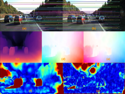
Figure 1: Inputs and intermediate CNN outputs of the system. (a, b) Current and previous input images with examples of auto-selected 2D-2D matches; (c) Single view depth prediction; (d, e) Forward and backward optical flow prediction; (f) Flow consistency between optical flow and rigid flow; (g) Forward-backward flow consistency; In (f)(g), red/blue means high/low inconsistency.

The ability of an autonomous robot to localize itself and know its surroundings is vital for different robotic tasks such as navigation and object manipulation. Vision-based methods are often the preferred choice because of factors such as cost-saving, low power requirements, and useful complementary information can be provided to other sensors such as IMU, GPS, laser scanners. We address the monocular Visual Odometry (VO) problem in this paper, where the goal is to estimate 6DoF motions of a moving camera.

Geometry-based Visual Odometry has shown dominating performance in the last few decades, while they are only reliable and accurate under a restrictive setup, such as when static scenes comprising well-textured Lambertian surfaces are captured with sufficient uniform illumination enabling to establish good correspondences Lowe (2004); Rublee et al. (2011); Bian et al. (2019a). The traditional correspondence search pipeline usually detects sparse feature points firstly and then matches extracted features, resulting in a limited number of high-quality correspondences because of the aforementioned assumptions. The accuracy and diversity of the correspondences are of the utmost importance in solving Visual Odometry problems. In contrast, we propose to extract accurate correspondences diversely from the dense predictions of an optical flow network using the consistency constraint between bi-directional flows. Then the selected correspondences are fed into geometry-based trackers (Epipolar Geometry based tracker and Prospective-n-point based tracker) for accurate and robust VO estimation, as described in Sec. 4.

Most monocular systems suffer from a depth-translation scale ambiguity issue, which means the predictions (structure and motion) are up-to-scale. The scale ambiguity leads to a scale drift issue that accumulated over time. Resolving scale-drift usually relies on keeping a scale-consistent map for map-to-frame tracking, performing an expensive global bundle adjustment for scale optimization or additional prior assumptions, like constant camera height from the known ground plane. Recently deep learning methods have made possible end-to-end learning of structure-and-motion from unlabelled videos. The trained single-view depth models give scale-consistent predictions with the use of stereo-based training Garg et al. (2016); Zhan et al. (2018); Godard et al. (2019) or scale-consistency constraint in monocular-based training Bian et al. (2019b). In this work, we propose to use the scale-consistent single-view depths as the reference to maintain a consistent scale over long videos. The scale-consistent depths are used in two circumstances: (1) scale recovery when the translation scale is missed in the Epipolar Geometry tracker; (2) establishing scale-consistent 3D-2D correspondences in the PnP tracker. Besides, we propose an iterative method for robust scale recovery, which is especially effective in highly dynamic scenes by removing the extracted correspondences (i.e. outliers) on dynamic regions.

Although recent deep pose networks can learn camera motions directly from videos Wang et al. (2017); Zhou et al. (2017); Zhan et al. (2018); Bian et al. (2019b); Godard et al. (2019), the accuracy is limited because of neglecting to incorporate geometric knowledge in inference time. In contrast, correspondences and scene scales are learnt in our proposed framework (Fig. 1). Thus accurate camera motions are estimated using well-studied multi-view geometry in the proposed system.

To summarize, the contributions of this paper include:

• we propose a hybrid system, DF-VO, which leverages both deep learning and multi-view geometry for Visual Odometry. Especially, self-supervised learning is used for training networks so expensive ground truth data is not required and it enables online finetuning.

• we propose to sample accurate sparse correspondences from dense optical flow predictions for camera tracking, and a bi-directional consistency based sampling method is presented.

• we propose to use scale-consistent monocular depth predictions for maintaining a consistent scale over long video for Visual Odometry, and propose an iterative scale recovery method for better performance in dynamic scenarios.

• the comprehensive evaluation shows that the proposed DF-VO system achieves state-of-the-art performance in standard benchmarks, and we conduct a detailed ablation study for evaluating the effect of different factors in our system.

A preliminary version of DF-VO was presented in Zhan et al. (2020). We extend the system in the following four aspects (1) clearer presentation and more details of the proposed system (2) improving the system in dynamic environments with an iterative correspondence selection scheme; (3) improving the adaptation ability in new environments by introducing an online adaptation scheme; (4) more comprehensive experiments and ablation studies.

2 Related Work

Geometry based VO: Camera tracking is a fundamental and well-studied problem in computer vision, with different pose estimation methods based on multiple-view geometry been established Hartley & Zisserman (2003); Scaramuzza & Fraundorfer (2011). Early work in VO dates back to the 1980s Ullman (1979); Scaramuzza & Fraundorfer (2011), with a successful application of it in the Mars exploration rover in 2004 Matthies et al. (2007), albeit with a stereo camera. Two dominant methods for geometry-based VO/SLAM are feature-based Mur-Artal & Tardós (2016); Klein & Murray (2007); Geiger et al. (2011) and direct methods Engel et al. (2017); Newcombe et al. (2011). The former involves explicit correspondence estimation, and the latter takes the form of an energy minimization problem based on the image colour/feature warp error, parameterized by pose and map parameters. There are also hybrid approaches that make use of the good properties of both Forster et al. (2014, 2016); Engel et al. (2014). One of the most successful and accurate full SLAM systems using a sparse (ORB) feature-based approach is ORB-SLAM2 Mur-Artal & Tardós (2016), along with DSO Engel et al. (2017), a direct keyframe-based sparse SLAM method. VISO2 Geiger et al. (2011) on the other hand is a feature-based VO system that only tracks against a local map created by the previous two frames. All these methods suffer from the previously mentioned issues (including scale-drift) common to monocular geometry-based systems. Various techniques have been developed for resolving the scale drift issue. For example, an expensive global bundle adjustment is performed for global scale optimization based on loop-closure detection, which does not always exist Mur-Artal et al. (2015b); or additional prior assumptions are introduced like constant camera height from the known ground plane Geiger et al. (2011); Zhou et al. (2019). In this work, with the aid of depth estimations from a consistent-scale deep network, scale estimation is performed with respect to the depth predictions such that a single consistent scale is maintained (Sec. 4.4).

Deep learning for VO: For supervised learning, Agrawal et al.Agrawal et al. (2015) propose to learn good visual features from an ego-motion estimation task, in which the model is capable of relative camera pose estimation. Wang et al.Wang et al. (2017) propose a recurrent network for learning VO from videos. Ummenhofer et al.Ummenhofer et al. (2017) and Zhou et al.Zhou et al. (2018) propose to learn monocular depth estimation and VO together in an end-to-end fashion by formulating structure from motion as a supervised learning problem. Dharmasiri et al.Dharmasiri et al. (2018) train a depth network and extend the depth system for predicting optical flows and camera motion. Recent works suggest that both tasks can be jointly learnt in a self-supervised manner using a photometric warp loss to replace a supervised loss based on ground truth. SfM-Learner Zhou et al. (2017) is the first self-supervised method for jointly learning camera motion and depth estimation. SC-SfM-Learner Bian et al. (2019b) is a very recent work which solves the scale inconsistent issue in SfM-Learner by enforcing depth consistency. Yin & Shi (2018); Ranjan et al. (2019) improve SfM-Learner by incorporating optical flow in their joint training framework for dynamics reasoning. Some prior works solve both scale ambiguity and inconsistency issue by using stereo sequences in training Li et al. (2017); Zhan et al. (2018), which address the issue of metric scale.

The issue with the above learning-based methods is that they do not explicitly account for the multi-view geometry constraints that are introduced due to camera motion during inference. In order to address this, recent works propose to combine the best of learning and geometry to varying extent and degree of success. CNN-SLAM Tateno et al. (2017) fuse single view CNN depths in a direct SLAM system, and CNN-SVO Loo et al. (2019) initialize the depth at a feature location with CNN provided depth for reducing the uncertainty in the initial map. Yang et al.Yang et al. (2018) feed depth predictions into DSO Engel et al. (2017) as virtual stereo measurements. Li et al.Li et al. (2019) refine their pose predictions via pose-graph optimisation. In contrast to the above methods, we effectively utilize CNNs for both single-view depth prediction and correspondence estimation, on top of standard multi-view geometry to create a simple yet effective VO system.

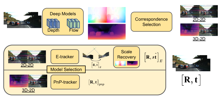
Figure 2: DF-VO pipeline. For an image pair, (forward and backward) optical flows and single view depths are predicted. A forward-backward flow consistency is computed as a criterion to establish good correspondences (2D-2D; 3D-2D). We have two alternative trackers out of which one is selected by the data-driven model selection module. The first tracker (E-tracker) uses 2D-2D correspondences to estimate and decompose an essential matrix to find rotation and translation direction, which is followed by a transnational scale recovery step to estimate metric VO. The second tracker (PnP) uses single view depth estimates in conjunction with 3D-2D registration via PnP.

3 Preliminaries

We revisit geometry-based pose estimation methods, including Epipolar Geometry and Perspective-n-Point in this section to understand the principle and the underlying limitations of each method.

3.1 Epipolar Geometry

Epipolar Geometry can be employed for camera motion estimation from two images ($I_{i},I_{j}$) Suppose we have obtained a set of 2D-2D correspondences ($\bm{p_{i}},\bm{p_{j}}$) from the image pair. Epipolar constraint is employed for solving fundamental matrix, $\bm{F}$, or essential matrix, $\bm{E}$, which are related by the camera intrinsic $\bm{K}$ such that $\bm{F}=\bm{K}^{-\bm{T}}\bm{E}\bm{K}^{-1}$. Thus, the camera motion $[\bm{R},\bm{t}]$ can be recovered by decomposing $\bm{F}$ or $\bm{E}$  Nister (2003); Zhang (1998); Hartley (1995); Bian et al. (2019c).

$$\bm{p_{j}}^{T}\bm{K}^{-\bm{T}}\bm{E}\bm{K}^{-1}\bm{p_{i}} =0,\text{ where }\bm{E}=[\bm{t}]_{\times}\bm{R}$$ (1)

However, the general viewpoint and general structure are assumed in such geometry guided tracking. Problems arise with Epipolar Geometry while frames in the sequence and/or scene structure do not conform to these assumptionsTorr et al. (1999).

• Motion degeneracy: motion degeneracy happens when the camera does not translate between frames, i.e. recovering $\bm{R}$ becomes unsolvable if the camera motion is a pure rotation.

• Structure degeneracy: viewed scene structure is planar.

Solving fundamental/essential matrix becomes unstable in practice when the camera baseline is small relative to the scene size. Moreover, translation recovered from the essential matrix is up-to-scale because of scale ambiguity.

3.2 Perspective-n-Point

Perspective-n-point (PnP) solves camera pose given known 3D-2D correspondences. In a two-view problem, suppose we have obtained a set of 3D-2D correspondences, including the 3D points on i-th view and the corresponding projection in j-th view $(\bm{X_{i}},\bm{p_{j}})$, PnP can be employed to estimate camera pose by minimizing the reprojection error,

$$e=\sum_{x}||\bm{K}(\bm{R}\bm{X}_{i}[\bm{x}]+\bm{t})-\bm{p}_{j}[\bm{x}]||_{2},$$ (2)

where $[\bm{x}]$ is pixel coordinate indexing. Solving a PnP problem requires accurate estimation of the 3D structure of the scene which can be obtained from depth sensor measurements or mature stereo reconstruction methods, while it is a more challenging problem in the monocular case.

4 DF-VO: Depth and Flow for Visual Odometry

4.1 System Overview

A standard Visual Odometry pipeline includes feature extraction and matching to establish correspondences , followed by pose estimation from the correspondences. We follow this pipeline and present DF-VO, which is illustrated in Fig. 2 and Alg. 1. Two types of correspondences (2D-2D and 3D-2D) are considered in this system. To obtain the correspondences, (1) an optical flow network is trained to predict dense correspondences between images for 2D-2D correspondences establishment; (2) a single-view depth network is used to estimate 3D structure thus 3D-2D correspondences can be established by combining the optical flow estimation. Accurate sparse correspondences are thus selected with a carefully designed mechanism. Two trackers used for pose estimation are named E-tracker and PnP-tracker, which employ Epipolar Geometry with a scale recovery module and Prospective-n-Point, respectively. Note that the scale recovery module is associated with E-tracker for solving the well-known scale ambiguity and scale drift issues. To decide a suitable tracker for each input pair, a robust model selection method using geometric robust information criterion is used. In order to achieve minimal training and supervision, and high-quality prediction on the deep networks, we explore a variety of training schemes on the depth network and flow network. Building on top of advanced deep networks and classic geometry methods, we present a simple yet effective and robust monocular Visual Odometry system.

4.2 Deep Predictions

In order to form 2D-2D/3D-2D correspondences from an image pair, specifically $(\bm{p_{i}},\bm{p_{j}})$ or $(\bm{X_{i}},\bm{p_{j}})$, we propose to use an optical flow network and a single-view depth network to establish the correspondences.

Optical flow

The 2D-2D correspondences are extracted from dense optical flow prediction. Give an image pair, $(I_{i},I_{j})$, optical flow describes the pixel movements in $I_{i}$, which gives the correspondences of all the pixels of $I_{i}$ in $I_{j}$. Though the state-of-the-art deep optical flow networks have shown high average accuracy, not all the pixels share the same high accuracy. Therefore, we propose a correspondence selection scheme in Sec. 4.3 to pick good predictions robustly.

Single view depth

In order to establish 3D-2D correspondences between two views, $(\bm{X_{i}},\bm{p_{j}})$, we need to obtain the 3D structure of i-th view and the correspondences between the 3D landmarks and 2D landmarks. Traditional approaches establish the correspondences via feature matching between 3D landmarks and 2D feature points. In this work, we use a deep depth network as our “depth sensor” to estimate the 3D structure on i-th view, $\bm{X_{i}}$. Through the 2D-2D correspondences established by optical flows, we can directly get a set of 3D-2D correspondences and solve the relative camera pose by solving PnP.

Unfortunately, the current state-of-the-art single view depth estimation methods are still insufficient for recovering very accurate 3D structure (about 10% relative error) for accurate camera pose estimation, which is shown in Tab. 3. On the other hand, optical flow estimation is a more generic task. The state-of-the-art deep learning methods are accurate and with good generalization ability. Therefore, we mainly use the 2D-2D matches for solving pose from essential matrix while the depth predictions are used for scale recovery and PnP-tracker. As a result, PnP-tracker is used as an auxiliary tracker when E-tracker tends to fail.

4.3 Correspondence Selection

Algorithm 1 DF-VO: Depth and Flow for Visual Odometry

1:Depth-CNN: $M_{d}$; Flow-CNN: $M_{f}$

2:Image sequence: $[\bm{I}_{1}$, $\bm{I}_{2}$, …, $\bm{I}_{k}]$

3:Camera poses: $[\bm{T}_{1},\bm{T}_{2},...,\bm{T}_{k}]$

4:Initialization $\bm{T_{1}}=\bm{I}$ ; $i=2$

5:while $i\leq k$ do

6:   Get CNN predictions: $\bm{D}_{i}$, $\bm{F}^{i}_{i-1}$, and $\bm{F}^{i-1}_{i}$

7:   Compute forward-backward flow inconsistency from ($\bm{F}^{i}_{i-1},\bm{F}^{i-1}_{i}$).

8:   Correspondence selection: form matches $(\bm{P}_{i},\bm{P}_{i-1})$ from the filtered flows based on flow inconsistency

9:   Model selection: estimate $\bm{E}$ and $\bm{H}$ from $(\bm{P}_{i},\bm{P}_{i-1})$ and compute GRIC scores for the trackers

10:   if E-Tracker then

11:      Recover $[\bm{R},\bm{\hat{\textbf{t}}}]$ from the estimated Essential matrix

12:      Triangulate $(\bm{P}_{i},\bm{P}_{i-1})$ to get $\bm{D}^{\prime}_{i}$

13:      Scale recovery to estimate $s$

14:      $\bm{T}^{i-1}_{i}=[\bm{R},s\bm{\hat{\textbf{t}}}]$

15:   else if PnP-Tracker then

16:      Form 3D-2D correspondences from $(\bm{D}_{i},\bm{P}_{i},\bm{P}_{i-1})$

17:      Estimate $[\bm{R},\bm{t}]$ using PnP

18:      $\bm{T}^{i-1}_{i}=[\bm{R},\bm{t}]$

19:   end if

20:   $\bm{T}_{i}\leftarrow\bm{T}_{i-1}\bm{T}^{i-1}_{i}$

21:end while

Most deep learning-based optical flow models predict dense optical flows, i.e. every pixel is associated with a predicted flow vector. There can be a lot of matches formed by the optical flows, in which some of them are very accurate. It is time-consuming if all matches are taken into consideration in solving a VO problem since only sparse matches are required to solve the problem in theory. The vanilla way is to sample the optical flows randomly/uniformly from the dense predictions.

However, we have observed that not all the flow predictions share the same high accuracy. Some regions in the images have worse optical flow predictions, for instance, out-of-view regions where no correspondences can be found in the other view; dynamic object regions where occlusion is usually associated with. In order to filter out the outliers and pick good optical flows, we propose a correspondence selection scheme based on a bi-directional flow consistency, see example in Fig. 3.

Flow consistency

Given an image pair, $(I_{i},I_{j})$, both forward and backward optical flows, $\bm{F}^{j}_{i}$ and $\bm{F}^{i}_{j}$, are predicted by the flow network. Thus we compute forward-backward flow consistency as a measure to choose good 2D-2D correspondences. The flow consistency is computed by,

$$\bm{C}=-\bm{F}^{j}_{i}-w\left(\bm{F}^{i}_{j},p_{f}(\bm{F}^{j}_{i})\right),$$ (3)

The warping process at a pixel $\bm{x}$ is described as

$$w\left(\bm{F}^{i}_{j}[\bm{x}],p_{f}(\bm{F}^{j}_{i}[\bm{x}])\right)=\bm{F}^{i}_{j}[\bm{x}+\bm{F}^{j}_{i}[\bm{x}]].$$ (4)

As $\bm{x}+\bm{F}^{i}_{j}[\bm{x}]$ does not necessarily locate on the regular grid, the resulted flow is interpolated from the flow vectors in the 4 cornersJaderberg et al. (2015). We use the flow consistency to select correspondences with higher accuracy and the hypothesis we made is that the optical flows with better consistency tend to have higher accuracy, which is proved with an experiment in Sec. 6.

Best-N selection

After computing forward-backward flow consistency, we choose optical flows with the least inconsistency $\bm{F^{\prime}}$ to form the best-N 2D-2D matches, $(\bm{P}_{i},\bm{P}_{j})$ Zhan et al. (2020), where N equals to 2000 in most experiments. This correspondence selection scheme is able to reject a lot of inaccurate flows. As shown in Zhan et al. (2020), DF-VO with this correspondence selection scheme has already outperformed existing VO/SLAM baselines. However, there are still some potential issues regarding the scheme.

• Model under-fitting: if the chosen best-N matches do not have enough location diversity, the pose model estimated can be an under-fitting model.

• Structure degeneracy: if all the chosen matches locate on a planar region, structure degeneracy happens and leads to the failure of estimating essential matrixTorr et al. (1999).

Local best-K selection

On top of the Best-N selection, we want to increase the location diversity of the matches. We divide the image regions into M ($M=10\times 10$) regions and choose best-K matches from each region. However, there might be cases that have severe inaccurate flow predictions (e.g. margin regions where usually are out-of-view) and the flow predictions should not be used. Therefore, we first filter the flows such that only flows with inconsistency less than a threshold can be picked. As a result, The final correspondences $(\bm{P_{i}},\bm{P_{j}})$ formed from $\bm{F^{\prime}}$ are a union of best-K matches in each region. The value K in j-th region is defined as $K_{j}=\text{min}(N/M,Q_{j})$, where $Q_{j}$ is the number of valid flows after thresholding. Since the correspondence quality is vital, we further check the number of valid correspondences and the number of regions with valid correspondences to determine if sufficient good correspondences are used. If insufficient correspondences are found, which rarely happens (mostly when the image quality is very poor such as extreme under/over-exposure), we use a constant motion model instead of the E/PnP-tracker.

The advantages of performing local best-K selection are two-fold, (1) increasing location diversity as described; (2) speeding up correspondence selection process since part of flows are rejected in the first place and sorting flow inconsistency is performed in a local image region instead of the whole image region.

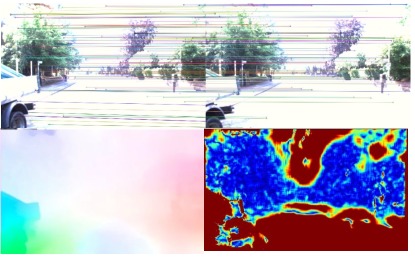
Figure 3: (Top) Filtered 2D correspondences established by the optical flow prediction; (Bottom left) Optical flow prediction; (Bottom right) Bidirectional flow consistency (high consistency is shown in blue) shows that sufficient correspondences can be established in the overexposure case.

Comparing to traditional feature-based methods, which only use salient feature points for matching and tracking, any pixel in the dense optical flow can be a candidate for tracking. Moreover, traditional features usually gather visual information from local regions while CNN gathers more visual information (larger receptive field) and higher-level contextual information, which gives more accurate and robust correspondences.

After selecting good 2D-2D correspondences, the essential matrix can be solved using Epipolar Geometry as described in Sec. 3.1. Then, the camera motion, consisting of rotation $\bm{R}$ and translation $\bm{\hat{\textbf{t}}}$, can be decomposed from the essential matrix. However, the recovered motion is up-to-scale. Specifically, the translation is a unit vector representing the translation direction only. In order to recover and maintain a consistent scale over the monocular footage, a consistent scale recovery process is required.

4.4 Scale Recovery

In traditional monocular VO pipeline, the per-frame scale is recovered by aligning triangulated 3D landmarks with existing 3D landmarks which accumulates errors.

Simple alignment

In this work, we use the predicted depths $\bm{D_{i}}$ to inform 3D structure as a reference for scale recovery. After recovering $[\bm{R},\bm{\hat{\textbf{t}}}]$ from solving essential matrix, triangulation is performed for $(\bm{P_{i}},\bm{P_{j}})$ to recover up-to-scale depths $\bm{D^{\prime}_{i}}$. A scaling factor, $s$, can be estimated by aligning the triangulated depth map $\bm{D^{\prime}_{i}}$ with the CNN depth map $\bm{D_{i}}$. An important advantage of using depth CNN is that we can get rid of the scale drift issue because of the following reasons.

• Depth CNN predicts per-frame 3D structures, which are scale consistent. We show that we can train scale consistent depth networks (Sec. 4.6).

• Scale drift is introduced by an accumulated error in creating new 3D landmarks. We do not create new 3D landmarks but recover scale w.r.t. a single network.

Iterative alignment

Algorithm 2 Iterative Scale Recovery

1:$[\bm{R},\bm{\hat{\textbf{t}}}]$, $\bm{F^{\prime}}$, $\bm{D}_{i}$, $s_{t-1}$

2:Initialization $s=s_{t-1}$

3:while s has not converged do

4:   Pose hypothesis: $\bm{T}=[\bm{R},s\bm{\hat{\textbf{t}}}]$

5:   Compute rigid flow $\bm{F}_{rigid}$ from $\bm{T}$ and $\bm{D}_{i}$

6:   Compute flow inconsistency: $\bm{F}_{diff}~{}\leftarrow~{}||\bm{F^{\prime}}-\bm{F}_{rigid}||_{2}$

7:   Select depth-flow pairs $(\bm{D}_{i},\bm{P}_{1},\bm{P}_{2})_{sel}$ with $\bm{F}_{diff}~{}<~{}\delta_{rigid}$

8:   Estimate new pose, $[\bm{R},\bm{\hat{\textbf{t}}}]$ from $(\bm{P}_{1},\bm{P}_{2})_{sel}$

9:   Triangulate $(\bm{P}_{1},\bm{P}_{2})_{sel}$ to get $\bm{D}^{\prime}_{i}$

10:   Estimate scaling factor, $s_{new}$, by comparing $(\bm{D}_{i,sel},\bm{D}^{\prime}_{i})$

11:   $s\leftarrow s_{new}$

12:end while

Aligning 3D landmarks triangulated on selected optical flow matches with CNN depths is simple and sufficient to recover accurate scale in general cases. However, in a highly dynamic environment, the selected optical flows can be lying on dynamic regions, which is problematic for depth alignment. Moreover, similar to optical flow predictions, not all the predicted depths are highly accurate. The pixels with high forward-backward flow consistency are not guaranteed to have high depth accuracy. Therefore, we here propose an iterative scheme, Alg. 2.

The key is to select depths and filtered optical flows (Sec. 4.3) that are consistent with each other. Given that the filtered optical flows generally establish good correspondences, a pixel with depth being consistent with the optical flow means that (1) the pixel belongs to a static region in the environment; (2) the depth is likely to be accurate. However, the depth and optical flow are related by a camera pose for a static scene. Since the camera pose $[\bm{R},\bm{\hat{\textbf{t}}}]$ is up-to-scale and does not share the same scale with the depth prediction, we, therefore, propose an iterative approach to select depth-flow pair (Alg. 2). We first initialize a relative pose $\bm{T}$ with a pose $\bm{T}_{0}$. Then the rigid flow is computed using the current relative pose by,

$$\bm{F}_{rigid}=\bm{K}\bm{T}\bm{K}^{-1}(\bm{x}\bm{D}_{i})-\bm{x}$$ (5)

where $\bm{x}$ belongs to pixel coordinates of the selected optical flow. The consistency between the filtered optical flow $\bm{F^{\prime}}$ and the rigid flow is then measured by $||\bm{F^{\prime}}-\bm{F}_{rigid}||_{2}$. Only depth-flow pairs with small optical-rigid flow inconsistency are selected as new matches. Thus, we update $\bm{T}$ with the new scaled pose and iterate the process until reaching the stopping condition (convergence or meet n-iterations). The scale initialization for the first image pair is set as zero while the scale at time-(t-1) is used as the scale initialization at time-(t).

4.5 Model Selection

We have presented a camera tracking method integrating Epipolar Geometry with deep predictions. However, as mentioned in Sec. 3.1, there are some known issues with Epipolar Geometry, i.e. motion degeneracy and unstable solution when the motion is small. Since we have both 3D-2D and 2D-2D correspondences available, we can instead solve a PnP problem using the correspondences obtained in Sec. 4.3 when Epipolar Geometry tends to fail. In this section, we show that we can select a suitable tracker/model by two possible ways.

Flow magnitude

We measure the magnitude of the flow predictions and solve essential matrix only when the average flow magnitude is large enough. It avoids small camera motions which usually come with small optical flowsZhan et al. (2020). However, this naïve approach is associated with some issues. (1) It does not resolve motion degeneracy (pure rotation), which also causes large optical flows. (2) It does not take outliers into account, e.g. dynamic objects which cause optical flows even the camera is stationary. Therefore, we adopt a more robust measure for model selection.

Geometric Robust Information Criterion

Torret al.Torr et al. (1999) discuss the degeneracy cases (motion and structure) and their influence on geometry guided camera motion estimation. Two robust strategies for tackling such degeneracies are proposed. (1) A statistical model selection test, named Geometric Robust Information Criterion (GRIC), is used to identify cases when degeneracies occur; (2) multiple motion models are used to overcome the degeneracies. In this work, we follow the first approach to identify when E-Tracker tends to fail and switch to PnP-Tracker. Torr et al. (1999) estimates both Fundamental $\bm{F}$ and Homography matrix $\bm{H}$ and choose the model with lower GRIC score. The model that explains the data best, i.e. lower GRIC score, is indicated as most likely.

GRIC calculates a score function for each tracker (Fundamental / Homography) considering the following factors.

• number of matches, $n$

• residuals of the matches, $e_{i}$

• standard deviation of the measurement error, $\sigma$

• data dimension, $r$ (4 for two views)

• number of motion model parameters, $k$ ($5$ for $\bm{E}$, $7$ for $\bm{F}$, 8 for $\bm{H}$)

• dimension of the structure, $d$ (3 for $\bm{F}$, 2 for $\bm{H}$)

$$\text{GRIC}=\sum\rho(e^{2}_{i})+\lambda_{1}dn+\lambda_{2}k$$ (6)

where $\rho(e^{2}_{i})$ is a robust function of the residuals:

$$\rho(e^{2})=\text{min}\left(\frac{e^{2}}{\sigma^{2}},\lambda_{3}(r-d)\right).$$ (7)

The value of the parameters are $\lambda_{1}=\text{log}4$, $\lambda_{2}=\text{log}4n$, $\lambda_{3}=2$. Different from Torr et al. (1999), since we have both 3D-2D and 2D-2D correspondences, we can choose PnP-Tracker instead of Homography-Tracker when E-Tracker tends to fail.

Cheirality condition

In addition to the two methods introduced above, we check for cheirality condition as well. There are 4 possible solutions for $[\bm{R},\bm{\hat{\textbf{t}}}]$ by decomposing $\bm{E}$. To find the correct unique solution, cheirality condition, i.e. the triangulated 3D points must be in front of both cameras, is checked to remove the other solutions. We further use the number of points satisfying cheirality condition as a reference to determine if the solution is stable.

Therefore, we choose PnP-Tracker when $\text{GRIC}_{E}$ is higher than $\text{GRIC}_{H}$ or cheirality check condition is not fulfilled. Otherwise, E-Tracker is employed for solving frame-to-frame camera motion. To robustify the system, we wrap the trackers in RANSAC loops.

4.6 Jointly learning of depths and pose

Various depth training frameworks can be employed depending on the availability of data (monocular/stereo sequences, depth sensor measurements). The most trivial way is using a supervised training framework Eigen et al. (2014); Liu et al. (2015, 2016); Laina et al. (2016); Kendall & Gal (2017); Nekrasov et al. (2019); Fu et al. (2018), but ground truth depths are not always available for any scenario. Some recent works suggest that jointly learning single-view depths and camera motion in a self-supervised manner is feasible using monocular sequences Zhou et al. (2017); Yin & Shi (2018); Godard et al. (2019); Bian et al. (2019b), or stereo sequences Garg et al. (2016); Godard et al. (2017); Zhan et al. (2018); Godard et al. (2019). Instead of using ground truth supervisions, the main supervision signal in the self-supervised framework is photometric consistency across multiple-views.

In this work, we mainly follow Godard et al. (2019) for training depth models using monocular and stereo sequences. The depth network is based on the encoder-decoder architecture with skip connectionsRonneberger et al. (2015). The pose network consists of a ResNet18 feature extractor which takes an image pair as input (concatenated as a 6-channel input) and predicts 6-DoF relative pose. We refer readers to Godard et al. (2019) for more network architecture details.

4.6.1 Training overview

In this work, we jointly train the depth network and the pose network by minimizing the mean of the following per-pixel objective function over the whole image. The per-pixel loss is

$$L= \min_{j}L_{pe}(\bm{I}_{i},\bm{I}^{i}_{j})+\lambda_{ds}L_{ds}(\bm{D}_{i},\bm{I}_{i})+$$

$$\min_{j}\lambda_{dc}L_{dc}(\bm{D}_{i},\bm{D}^{i}_{j}),$$ (8)

where $L_{pe}$ is photometric loss; $L_{ds}$ is depth smoothness loss; $L_{dc}$ is depth consistency loss; and $[\lambda_{ds},\lambda_{dc}]$ are loss weightings.

4.6.2 Photometric loss

$L_{pe}$ is the photometric error by computing the difference between the reference image $\bm{I}_{i}$ and the synthesized view $\bm{I}^{i}_{j}$ warped from the source image $\bm{I}_{j}$, where $j\in[i-n,i+n,s]$. $[i-n,i+n]$ are neighbouring views of $I_{i}$ while $s$ is stereo pair if stereo sequences are used in training. As proposed in Godard et al. (2019), instead of averaging the photometric errors between the reference pixel and the synthesized pixels from multiple views, Godard et al. (2019) only counts the photometric error between the reference pixel and the synthesized pixel with the minimum error. The rationale is to overcome the issues related to out-of-view pixels and occlusions.

$$L_{pe}(\bm{I}_{i},\bm{I}^{i}_{j}) =\frac{\alpha}{2}\left(1-\text{SSIM}(\bm{I}_{i},\bm{I}^{i}_{j})\right)+(1-\alpha)|\bm{I}_{i}-\bm{I}^{i}_{j}|$$ (9)

$$\bm{I}^{i}_{j} =w\left(\bm{I}_{j},p_{re}(\bm{K},\bm{D}_{i},\bm{T}^{j}_{i})\right),$$ (10)

where SSIM Wang et al. (2004) is a robust measurement for image similarity and $\alpha=0.85$ balances the SSIM error and the simple color intensity error. $w(\bm{I},\bm{p})$ is a differentiable warping function Jaderberg et al. (2015) which warps image $\bm{I}$ according to the pixel locations $\bm{p}$. $p_{re}(\bm{K},\bm{D}_{i},\bm{T}^{j}_{i})$ establishes the pixel coordinates reprojected from view-i to view-j, where $\bm{K}$ is the camera intrinsics, $\bm{D}_{i}$ is the predicted depth map of view-i, and $\bm{T}^{j}_{i}$ is the relative pose between the pair. The reprojection for a pixel $\bm{x}$ from view-i to view-j is represented by

$$p_{re}\left(\bm{K},\bm{D}_{i},\bm{T^{j}_{i}}\right)=\bm{K}\bm{T^{j}_{i}}\bm{K^{-1}}\bm{x}\bm{D}_{i}[\bm{x}]$$ (11)

4.6.3 Depth smoothness regularization

Following the approach in Godard et al. (2017), we encourage depth to be smooth locally so we induce an edge-aware depth smoothness term. The depth discontinuity is penalized if colour continuity is presented in the same local region. The smoothness regularization is formulated as

$$L_{ds}(\bm{D}_{i},\bm{I}_{i})=|\partial_{x}\bm{D}_{i}|e^{-|{\partial_{x}\bm{I}_{i}}|}+|\partial_{y}\bm{D}_{i}|e^{-|{\partial_{y}\bm{I}_{i}}|},$$ (12)

where $\partial_{x}(.)$ and $\partial_{y}(.)$ are gradients in horizontal and vertical direction respectively. Note that we use inverse depth regularization instead.

4.6.4 Training without scaling issues

Similar to traditional monocular 3D reconstruction, scale ambiguity and scale inconsistency issues exist when monocular videos are used for training. Since the monocular training usually uses image snippets (usually 2 or 3 frames) for training, the training does not guarantee a consistent learnt scale across snippets and it creates the scale inconsistency issueBian et al. (2019b).

One solution to solve both scale problems is using stereo sequences during training Li et al. (2017); Zhan et al. (2018); Godard et al. (2019), the deep predictions are aligned with real-world scale and scale-consistent because of the constraint introduced by the known stereo baseline. Even though stereo sequences are used during training, only monocular images are required during inference for depth predictions.

Another solution to overcome the scale inconsistency issue is using temporal geometry consistency regularization proposed in Zhan et al. (2019); Bian et al. (2019b), which constrains the depth consistency across multiple views. As depth predictions are consistent across different views and thus different snippets, the scale inconsistency issue is resolved. Using the rigid scene assumption as the cameras move in space over time we want the predicted depths at view-i to be consistent with the respective predictions at view-j. This is done by correctly transforming the scene geometry from frame-$j$ to frame-$i$ much like the image warping. Specifically, we adopt the inverse depth consistency proposed in Zhan et al. (2019).

$$L_{dc}(\bm{D}_{i},\bm{D}^{i}_{j})=|1/\bm{D}_{i}-1/\bm{D}^{i}_{j}|$$ (13)

Inspired by Godard et al. (2019), we use minimum error in multi-view pairs to avoid occlusions and out-of-view scenes instead of averaging the depth consistency error over all source views.

4.7 Learning of optical flows

Many deep learning-based methods have been proposed for estimating optical flow Dosovitskiy et al. (2015); Ilg et al. (2017); Hui et al. (2018); Sun et al. (2018); Meister et al. (2018). In this work, we choose LiteFlowNetHui et al. (2018) as our backbone network for optical flow prediction since LiteFlowNet is fast, lightweight, and accurate. LiteFlowNet consists of a two-stream network for feature extraction and a cascaded network for flow inference and regularization. We refer readers to Hui et al. (2018) for more details. LiteFlowNet shows good generalization ability. LiteFlowNet trained on a synthetic dataset (Scene FlowDosovitskiy et al. (2015)) can generalize well in real-world scenarios, though sometimes artifacts present in some regions.

In this work, we mainly use the model trained from Scene Flow. However, we also show that a self-supervised finetuning can be performed to help the model better adapt to unseen environments and remove the artifacts. Two finetuning schemes are tested and compared, including offline finetuning and online finetuning (Sec. 6.2). Similar to the self-supervised training of the depth network, the optical flow network is trained by minimizing the mean of the following per-pixel loss function over the whole image.

$$L= \min_{j}L_{pe}(\bm{I}_{i},\bm{I}^{i}_{j})+\lambda_{fs}L_{fs}(||\bm{F}^{j}_{i}||_{2},\bm{I}_{i})$$

$$+\lambda_{fc}L_{fc}\left(\left|-\bm{F}^{j}_{i}-w\left(\bm{F}^{i}_{j},p_{f}(\bm{F}^{j}_{i})\right)\right|\right)$$ (14)

$$\bm{I}^{i}_{j} =w\left(\bm{I}_{j},p_{f}(\bm{F}^{j}_{i})\right),$$ (15)

Different from Eqn. 10, $p_{f}(.)$ establish the correspondences between view-i and view-j via the flow field instead of using reprojection defined in Eqn. 10. For a pixel $\bm{x}$ on view-i, the corresponding pixel position , $p_{f}(\bm{F}^{j}_{i}[\bm{x}])$, on view-j is $\bm{x}+\bm{F}^{j}_{i}[\bm{x}]$.

We also regularize the optical flow to be smooth using an edge-aware flow smoothness loss $L_{fs}(.)$ similar to the depth smoothness loss defined in Eqn. 12. Similar to Meister et al.Meister et al. (2018), we estimate both forward and backward optical flow and constrain the bidirectional predictions to be consistent with the loss $L_{fc}$.

5 Implementation and Benchmarking

5.1 Dataset

We train and test our method in popular benchmarking datasets, KITTI Geiger et al. (2012, 2013) and Oxford RobotcarMaddern et al. (2017), which are large scale outdoor driving datasets. There are various splits in KITTI for several tasks, e.g. depth estimation, odometry, object tracking. In this work, we select the following three splits to evaluate our method.

KITTI Odometry

Odometry split contains 11 driving sequences with publicly available ground truth camera poses. Most of the sequences are long sequences and some with loop closing. Following Zhou et al. (2017), we train our networks on sequences 00-08. The dataset contains 36,671 training pairs, [$I_{i},I_{i-1},I_{i+1},I_{i,s}$].

KITTI Tracking

Tracking split contains 21 sequences with available ground truths. The split is primarily used for object tracking benchmarking so there are more dynamic objects in these sequences when compared to the Odometry split, but shorter sequence length in general. Following Zhang et al. (2020), we choose 9 out of the 21 sequences with a considerable number of dynamic objects to test the robustness of our system in dynamic environments. These sequences are challenging for most monocular VO/SLAM systems since most of the systems assume static scenarios.

KITTI Flow

KITTI Flow 2012/2015 splits contain 194/200 image pairs with high-quality optical flow labels. We use this split to evaluate the performance of the optical flow models in this work.

Oxford Robotcar

To further test the generalization ability of the system, we test the proposed system on Oxford Robotcar dataset. Following Loo et al. (2019), 8 sequences are selected for evaluation and the first 200 frames are skipped in the evaluation due to the extremely overexposed images at the beginning of the sequences.

5.2 Deep network training

We train our networks with the PyTorch Paszke et al. (2017) framework. All self-supervised experiments are trained using Adam optimizer Kingma & Ba (2014) for 20 epochs. For KITTI, images with a size of 640 $\times$ 192 are used for training. Learning rate is set to $10^{-4}$ for the first 15 epochs and then is dropped to $10^{-5}$ for the remaining epochs. The loss weightings are $[\lambda_{ds},\lambda_{dc}]=[10^{-3},5]$ for jointly learning depths and camera motion while $[\lambda_{fs},\lambda_{fc}]=[10^{-1},5\times 10^{-3}]$ for optical flow experiments.

5.3 Visual Odometry Benchmarking

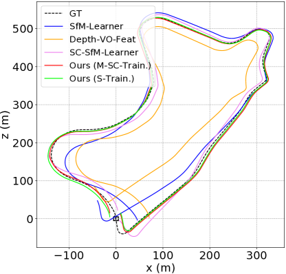
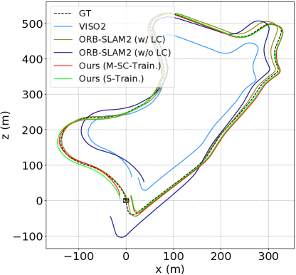
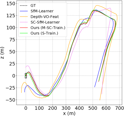
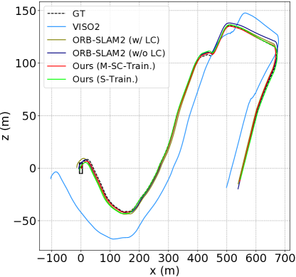
Figure 4: Qualitative VO results on KITTI: (Top) Seq.09 and (Bottom) Seq.10 against deep learning-based and geometry-based methods (shown separately).

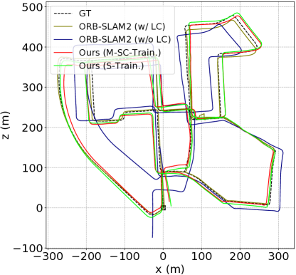
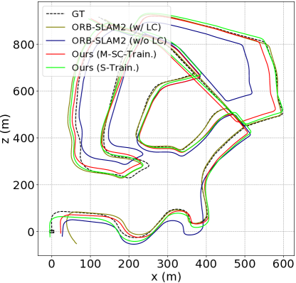
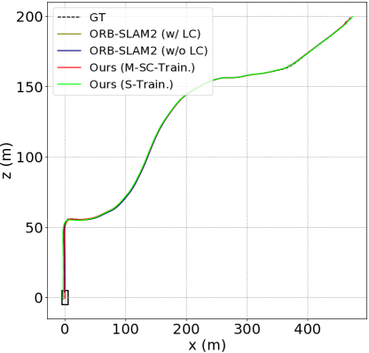
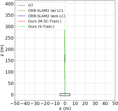
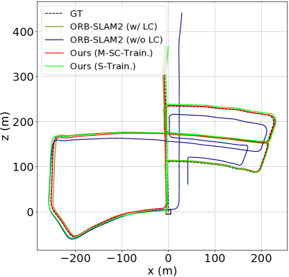
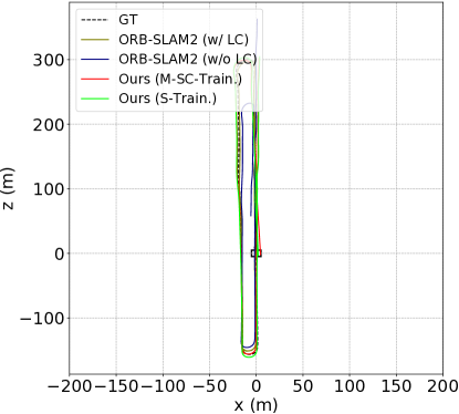
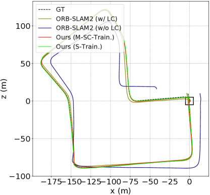
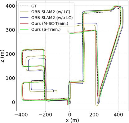
Figure 5: DF-VO and ORB-SLAM2 (monocular, w/ and w/o loop-closure) trajectories in sequences 00, 02, 03, 04, 05, 06, 07 and 08 from the KITTI odometry benchmark. Note that Seq. 08 does not contains loops and ORB-SLAM2 (w/ LC) undergoes severe scale drifting while DF-VO does not.

Table 1: Quantitative result on KITTI Odometry Seq. 00-10. The best result is in bold and second best is underlined.

Category	Method	Metric	00	01	02	03	04	05	06	07	08	09	10	Avg. Err.
Deep VO	SfM-Learner Zhou et al. (2017)	$t_{err}$	21.32	22.41	24.10	12.56	4.32	12.99	15.55	12.61	10.66	11.32	15.25	14.068
		$r_{err}$	6.19	2.79	4.18	4.52	3.28	4.66	5.58	6.31	3.75	4.07	4.06	4.660
		ATE	104.87	109.61	185.43	8.42	3.10	60.89	52.19	20.12	30.97	26.93	24.09	51.701
		RPE (m)	0.282	0.660	0.365	0.077	0.125	0.158	0.151	0.081	0.122	0.103	0.118	0.158
		RPE (∘)	0.227	0.133	0.172	0.158	0.108	0.153	0.119	0.181	0.152	0.159	0.171	0.160
	Depth-VO-Feat Zhan et al. (2018)	$t_{err}$	6.23	23.78	6.59	15.76	3.14	4.94	5.80	6.49	5.45	11.89	12.82	7.911
		$r_{err}$	2.44	1.75	2.26	10.62	2.02	2.34	2.06	3.56	2.39	3.60	3.41	3.470
		ATE	64.45	203.44	85.13	21.34	3.12	22.15	14.31	15.35	29.53	52.12	24.70	33.220
		RPE (m)	0.084	0.547	0.087	0.168	0.095	0.077	0.079	0.081	0.084	0.164	0.159	0.108
		RPE (∘)	0.202	0.133	0.177	0.308	0.120	0.156	0.131	0.176	0.180	0.233	0.246	0.193
	SC-SfMLearner Bian et al. (2019b)	$t_{err}$	11.01	27.09	6.74	9.22	4.22	6.70	5.36	8.29	8.11	7.64	10.74	7.803
		$r_{err}$	3.39	1.31	1.96	4.93	2.01	2.38	1.65	4.53	2.61	2.19	4.58	3.023
		ATE	93.04	85.90	70.37	10.21	2.97	40.56	12.56	21.01	56.15	15.02	20.19	34.208
		RPE (m)	0.139	0.888	0.092	0.059	0.073	0.070	0.069	0.075	0.085	0.095	0.105	0.086
		RPE (∘)	0.129	0.075	0.087	0.068	0.055	0.069	0.066	0.074	0.074	0.102	0.107	0.083
VO with Optim.	DSO Engel et al. (2017)	ATE	113.18	/	116.81	1.39	0.42	47.46	55.62	16.72	111.08	52.23	11.09	52.600
Full SLAM /	ORB-SLAM2 (w/o LC) Mur-Artal & Tardós (2016)	$t_{err}$	11.43	107.57	10.34	0.97	1.30	9.04	14.56	9.77	11.46	9.30	2.57	8.074
		$r_{err}$	0.58	0.89	0.26	0.19	0.27	0.26	0.26	0.36	0.28	0.26	0.32	0.304
		ATE	40.65	502.20	47.82	0.94	1.30	29.95	40.82	16.04	43.09	38.77	5.42	26.480
		RPE (m)	0.169	2.970	0.172	0.031	0.078	0.140	0.237	0.105	0.192	0.128	0.045	0.130
		RPE (∘)	0.079	0.098	0.072	0.055	0.079	0.058	0.055	0.047	0.061	0.061	0.065	0.063
	ORB-SLAM2 (w/ LC) Mur-Artal & Tardós (2016)	$t_{err}$	2.35	109.10	3.32	0.91	1.56	1.84	4.99	1.91	9.41	2.88	3.30	3.247
		$r_{err}$	0.35	0.45	0.31	0.19	0.27	0.20	0.23	0.28	0.30	0.25	0.30	0.268
		ATE	6.03	508.34	14.76	1.02	1.57	4.04	11.16	2.19	38.85	8.39	6.63	9.464
		RPE (m)	0.206	3.042	0.221	0.038	0.081	0.294	0.734	0.510	0.162	0.343	0.047	0.264
		RPE (∘)	0.090	0.087	0.079	0.055	0.076	0.059	0.053	0.050	0.065	0.063	0.066	0.066
VO	VISO2 Geiger et al. (2011)	$t_{err}$	10.53	61.36	18.71	30.21	34.05	13.16	17.69	10.80	13.85	18.06	26.10	19.316
		$r_{err}$	2.73	7.68	1.19	2.21	1.78	3.65	1.93	4.67	2.52	1.25	3.26	2.519
		ATE	79.24	494.60	70.13	52.36	38.33	66.75	40.72	18.32	61.49	52.62	57.25	53.721
		RPE (m)	0.221	1.413	0.318	0.226	0.496	0.213	0.343	0.191	0.234	0.284	0.442	0.297
		RPE (∘)	0.141	0.432	0.108	0.157	0.103	0.131	0.118	0.176	0.128	0.125	0.154	0.134
	Ours (Mono-SC Train.)	$t_{err}$	2.33	39.46	3.24	2.21	1.43	1.09	1.15	0.63	2.18	2.40	1.82	1.848
		$r_{err}$	0.63	0.50	0.49	0.38	0.30	0.25	0.39	0.29	0.32	0.24	0.38	0.367
		ATE	14.45	117.40	19.69	1.00	1.39	3.61	3.20	0.98	7.63	8.36	3.13	6.344
		RPE (m)	0.039	1.554	0.057	0.029	0.046	0.024	0.030	0.021	0.041	0.051	0.043	0.038
		RPE (∘)	0.056	0.049	0.045	0.038	0.029	0.035	0.029	0.030	0.037	0.036	0.043	0.038
	Ours (Stereo Train.)	$t_{err}$	2.01	40.02	2.32	2.22	0.74	1.30	1.42	0.72	1.66	2.07	2.06	1.652
		$r_{err}$	0.61	0.47	0.48	0.30	0.25	0.30	0.32	0.35	0.33	0.23	0.36	0.353
		ATE	12.17	342.71	17.59	1.96	0.70	4.94	3.73	1.06	6.96	7.59	4.21	6.091
		RPE (m)	0.025	0.854	0.030	0.021	0.026	0.018	0.025	0.015	0.030	0.044	0.040	0.027
		RPE (∘)	0.055	0.052	0.045	0.038	0.029	0.035	0.030	0.031	0.036	0.037	0.043	0.038

Evaluation Criterion

Some common evaluation criteria are adopted for a detailed analysis. KITTI Odometry criterion reports the average translational error $t_{err}(\%)$ and rotational errors $r_{err}(^{\circ}/100m)$ by evaluating possible sub-sequences of length (100, 200, …, 800) meters. Absolute trajectory error (ATE) measures the root-mean-square error between predicted camera poses $[x,y,z]$ and ground truth. Relative pose error (RPE) measures frame-to-frame relative pose error. Since most of the methods are a monocular method, which lacks a scaling factor to match with the real-world scale, we scale and align (7DoF optimization) the predictions to the ground truth associated poses during evaluation by minimizing ATE Umeyama (1991). Except for methods using stereo depth models (Ours(Stereo Train.), Depth-VO-Feat) and known scale prior (VISO2), which have already aligned predictions to real-world scale, for a fair comparison, we perform 6DoF optimization w.r.t ATE instead.

KITTI Odometry

We provide a detailed comparison between our VO system and some prior arts in KITTI Odometry split, which includes pure deep learning methods Zhou et al. (2017), Zhan et al. (2018) Bian et al. (2019b), and geometry-based methods including DSOEngel et al. (2017), VISO2Geiger et al. (2011), and ORB-SLAM2 Mur-Artal et al. (2015a) (w/ and w/o loop-closure). ORB-SLAM2 occasionally suffers from tracking failure or unsuccessful initialization. We run ORB-SLAM2 three times and report the one with the least trajectory error. The quantitative and qualitative results are shown in Tab. 1, Fig. 4, and Fig. 5. Seq.01 is not included while computing average error since a sub-sequence of Seq.01 does not contain trackable close features and most methods fail in the sub-sequence.

Ours (Mono-SC Train.) uses a depth model trained with monocular videos and inverse depth consistency for ensuring scale-consistency. Ours (Stereo Train) uses a depth model trained with stereo videos. Note that even stereo sequences are used during training, monocular sequences are used in testing. Therefore, Ours (Stereo Train) is still a monocular VO system. We show that our methods outperform pure deep learning methods, which rely on a PoseCNN for camera motion estimation, by a large margin in all metrics. For KITTI Odometry criterion, ORB-SLAM2 shows less rotation drift $r_{err}$ but higher translation drift $t_{err}$ due to scale drift issue, which is also showed in Fig. 4. The drifting issue sometimes can be resolved by loop closing with expensive global bundle adjustment but the issue exists when there is no loop closing detected. Different from other methods, we use a single depth network as our “reference map”. The translation scales are recovered w.r.t to the scale-consistent depth predictions. As a result, we mitigate the scale drift issue in most monocular VO/SLAM systems and show less translation drift over long sequences. More importantly, our method shows a consistently smaller relative error, both translation and rotation, which allows our system to be a robust module for frame-to-frame tracking.

KITTI Tracking

To show the robustness of our system in dynamic environments, we compare our system with ORB-SLAM2 in KITTI Tracking dataset individually. The results are shown in Tab. 5. However, since the Tracking split contains relatively shorter sequences when compared to the Odometry split, KITTI Odometry criterion is not a suitable measurement to evaluate the performance. Therefore, we report frame-to-frame RPE (translation) for Tracking split as a reference. Note that sequence (2011/10/03-47) is the most difficult sequence among the 9 sequences due to its highly dynamic environment in a highway. ORB-SLAM2 is well known for its superior ability in removing outliers but its performance still downgraded significantly in this sequence while our method performs robustly.

Table 2: Visual odometry evaluation in Oxford Robotcar Dataset. Absolute Trajectory Error (metre) is used as the evaluation criterion.

Sequence	SVO	CNN-SVO	DSO	ORB-SLAM (w/o LC)	Ours
	Forster et al. (2016)	Loo et al. (2019)	Engel et al. (2017)	Mur-Artal et al. (2015b)
2014-05-06-	X	8.66	4.71	10.66	4.16
12-54-54
2014-05-06-	X	9.19	X	X	3.46
13-09-52
2014-05-06-	X	10.19	X	X	4.55
13-14-58
2014-05-06-	X	8.26	X	X	4.58
13-17-51
2014-05-14-	X	13.75	X	X	6.89
13-46-12
2014-05-14-	X	6.30	X	X	5.09
13-53-47
2014-05-14-	X	6.15	2.45	X	1.83
13-59-05
2014-06-25-	X	3.70	X	6.56	3.20
16-22-15

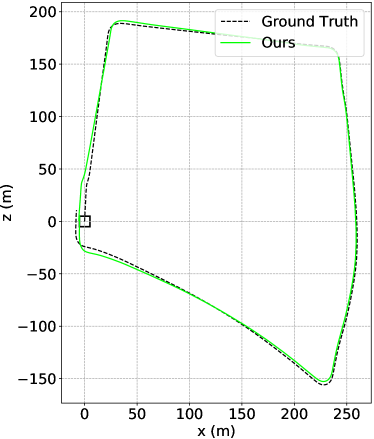
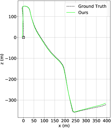
Figure 6: Qualitative VO results on Oxford Robotcar: (Left) 2014-05-06-12-54-54 and (Right) 2014-06-25-16-22-15. Note that there is in fact a loop closure in the left sequence but the ”Ground truth” is not accurate enough as mentioned in the Robotcar official document.

Oxford Robotcar

We also test the generalization ability of the system on Oxford RobotcarMaddern et al. (2017). The result is reported in Tab. 2 and illustrated in Fig. 6. Note that there are some overexposed frames at the middle of the sequence (e.g. Fig. 3), which are challenging for visual odometry/SLAM algorithms such that many algorithms listed in Tab. 2 fail to run the sequences. However, the deep optical flow network still predicts sufficient good correspondences for pose estimation (Fig. 3). The optical network rarely fails to give sufficient good correspondences but the number of valid correspondences reflects the failure cases and constant motion model is employed in such cases. The result shows that our system outperforms the others. More importantly, it proves that sampling correspondence from deep optical flow is more robust than matching hand-crafted features.

6 Ablation study

Table 3: Ablation study on KITTI Odometry dataset regarding different components

Experiment	Variant	09		10
		$t_{err}$	$r_{err}$	$t_{err}$	$r_{err}$
Reference Model		3.45	0.68	3.19	1.00
Tracker	PnP	6.79	2.27	6.31	3.75
Flow	Self-Flow (Offline)	2.90	0.74	2.98	1.03
	Self-Flow (Online)	2.07	0.38	2.54	0.62
Depth	Mono-SC	3.45	0.73	3.63	1.20
	Mono.	3.52	0.81	4.29	1.44
Correspondences	Uniform	5.05	1.18	5.38	1.97
	Best-N	4.88	1.06	4.26	1.83
Scale	Iterative	3.34	0.63	3.05	1.07
Model Sel.	Flow	3.71	0.76	3.57	1.16
Img. Res.	Full	2.38	0.37	2.00	0.40

In this section, we present an extensive ablation study (Tab. 3) to understand the effect of the components proposed in this work. We use a Reference Model with the following settings and study the component in the following categories.

• Tracker: Hybrid (E-tracker and PnP-tracker)

• Depth model: Trained with stereo sequences

• Flow model: LiteFlowNet trained from synthetic dataset

• Correspondence selection: Local best-K selection

• Scale recovery: Simple alignment

• Model selection: GRIC

• Image resolution: down-sampled size ($640\times 192$)

6.1 Tracker

DF-VO consists of two trackers – E-tracker and PnP-tracker. E-tracker is considered as the main tracker when general motion (sufficient translation) and general structure (non-planar) are assumed. PnP-tracker is used when E-tracker fails to estimate the motion, which is introduced in Sec. 4.5. Using E-tracker alone potentially fails when motion degeneracy or structure degeneracy happens as described in Sec. 3.1. Therefore, we only compare the Reference model to the case that only PnP-tracker is used. PnP relies on the accuracy of both depth and optical flow predictions for establishing accurate 3D-2D correspondence. However, there is not a straightforward way to sample good depth predictions for accurate 3D-2D correspondences for 6DoF pose estimation, but the depth predictions are sufficient for 1DoF scale recovery problem in E-tracker.

6.2 Flow model

Table 4: Optical flow evaluation in KITTI 2012/2015 optical flow split. Average end-point-error (AEPE) and the percentage of pixels with error larger than 1 (Out-1) are evaluated. Non-occluded regions are evaluated. SF (Super.): supervised training on Scene Flow. KITTI (Self.): self-supervised training on KITTI. BestN: Bidirectional flow consistency thresholding is applied.

Network	Dataset & Method	KITTI 2012		KITTI 2015
		AEPE (px)	Out-1 (%)	AEPE (px)	Out-1 (%)
LiteFlowNet	SF (Super.)	1.593	26.1%	4.785	39.6%
LiteFlowNet	SF (Super.) + KITTI (Self.)	1.467	19.7%	4.987	32.7%
LiteFlowNet	SF (Super.) + BestN	0.478	7.6%	0.711	10.5%
LiteFlowNet	SF (Super.) + KITTI (Self.) + BestN	0.422	5.7%	0.628	7.7%

LiteFlowNet trained with synthetic data shows acceptable generalization ability from synthetic to real. However, there are still some regions with significantly erroneous flow predictions. We find that with self-supervised finetuning, the model adapts better to the real world sequences and the optical flow prediction accuracy is improved (Tab. 4).

offline v.s. online

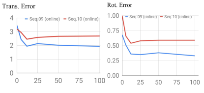
Figure 7: Effect of self-supervised online finetuning. X-axis is the percentage of data used in the online finetuning.

We perform two types of self-supervised finetuning for the optical flow network. The offline method finetunes the flow network on sequences 00-08 using monocular videos while the online method finetunes the model on-the-run for the running sequence. We test various amounts of data for online finetuning and evaluate the corresponding odometry result. The relationship is shown in Fig. 7. We can see that finetuning on a small amount of data (10%) is sufficient for the optical flow network to adapt to unseen scenarios.

Flow evaluation

We evaluate the quality of optical flows on KITTI 2012/2015, which are two benchmark dataset for optical flow evaluation. The result is shown in Tab. 4. We can see that with self-supervised finetuning (offline), the accuracy of the flow prediction is significantly improved, especially in the percentage of outliers. One noticeable result is that self-supervised training increases the end-point-error in KITTI2015 from 4.785 to 4.987. The reason is that the self-supervised model is trained in KITTI Odometry split, which contains long driving sequences without many dynamic objects. However, KITTI2015 contains many dynamic objects and we observe that the error of the flow estimation on these dynamic objects are larger for the self-supervised model, which increases the average error. On the other hand, Scene Flow model is trained in highly dynamic synthetic environments, i.e. able to estimate large flow magnitude caused by moving objects. Moreover, the synthetic model generates artifacts in some regions when used in real-world data so there are more outliers, as shown in Tab. 4. Nevertheless, the correspondence selection module effectively removes the bad flows predicted by the self-supervised model and the overall flow accuracy is improved over the Scene Flow model. Since better correspondences are estimated, the odometry result using Self-Flow is improved as well.

6.3 Depth model

Training depth models with monocular videos comes with a scale inconsistency issue Bian et al. (2019b). We use an inverse depth consistency proposed in Zhan et al. (2019) to enforce the depth predictions to be consistent (Sec. 4.6.4). Using a scale-consistent depth CNN for translation scale recovery helps to mitigate the scale drift issue, which usually occurs after long travelling. Here we compare three depth models trained by different strategies. We train two models using monocular videos. Mono. model is trained without the depth consistency term while Mono-SC model is trained with the depth consistency term. Models trained with monocular videos are always up-to-scale, i.e. the metric scale is unknown. Therefore, we also train a model using stereo sequences. Note that, the model trained with stereo sequences do not include the depth consistency term. The predictions in stereo training are always associated with one and only one scale i.e. real-world scale due to the constraint set by the known stereo baseline. Therefore, no scale ambiguity/inconsistency issues exist in this training scheme. We can see that both Reference Model (stereo) and Mono-SC have less $t_{err}$ and $r_{err}$ after long travelling, which is aided by the scale-consistent depth predictions.

We also explored an online adaptation scheme for the depth network. However, the depth network training is unstable in the online finetuning. The scale of the depth predictions fluctuates during the training due to the scale ambiguity nature in the monocular training.

6.4 Correspondence selection

Since only sparse matches are required for DF-VO, a naïve way to extract sparse matches from dense optical flow prediction is to sample matches uniformly/randomly. We uniformly sampled 2000 flows to form the correspondences and it shows that the odometry result is worse than either Best-N selection or Local Best-K selection method. To verify the effectiveness of forward-backward flow inconsistency, which is used for correspondences selection in both Best-N selection and Local Best-K selection, we evaluate the optical flow performance with/without the selection (Tab. 4). Instead of evaluating best-N points, we alternatively set an inconsistency threshold such that only the flows with inconsistency less than $\delta_{fc}$ are evaluated. We show that the accuracy of the selected flows is improved significantly when compared to the average result of all optical flows.

6.5 Scale recovery

Table 5: Quantitative result on KITTI tracking sequences. The RPE (m) is reported.

Seq.	Seq. Length	ORB-SLAM2	DF-VO (Ours)
	(m)		Simple	Iterative
2011/09/26-05	69.4	0.053	0.039	0.038
2011/09/26-09	332.4	0.061	0.049	0.047
2011/09/26-11	114.0	0.033	0.030	0.030
2011/09/26-13	173.0	0.075	0.071	0.071
2011/09/26-14	402.5	0.101	0.074	0.074
2011/09/26-15	362.8	0.087	0.068	0.063
2011/09/26-18	51.5	0.049	0.014	0.015
2011/09/29-04	254.9	0.073	0.040	0.044
2011/10/03-47	712.6	0.200	0.071	0.060
Average	274.8	0.081	0.051	0.049

We propose two scale recovery methods in this work, namely simple alignment and Iterative alignment. Simple alignment aligns the triangulated depths of the filtered optical flows and their corresponding depth predictions. However, the filtered optical flows can fall onto dynamic object regions and the depth predictions may not be accurate. The iterative alignment is proposed for more robust scale recovery in dynamic environments. Only depth points and filtered optical flows that are consistent with each other are used for scale recovery. This eliminates both bad depth predictions and optical flows of the dynamic objects. Iterative alignment slightly improves over the simple alignment in KITTI Odometry split, which might be because of the less dynamic scene nature of the sequences. However, in a highly dynamic environment, like KITTI Tracking split, especially in Seq. 2011/10/03-47 which is a sequence on a highway with one-third of the image occupied by moving cars, iterative scale recovery shows a better result when compared to simple alignment and works more robustly when compared to ORB-SLAM2 (Tab. 5).

6.6 Model selection

Two model selection methods are proposed and tested in this work. Flow magnitude-based method Zhan et al. (2020) is straightforward but there are some potential failure cases, which is explained in Sec. 4.5. Moreover, a flow magnitude thresholding value is required in this method, which is found empirically. However, GRIC-based model selection is a parameter-free method, which calculates a score function for each motion model. It shows a more robust result when compared to the flow-based method.

6.7 Image resolution

Down-sampled images are used in the Reference Model because the size is used in training deep networks. However, simply increasing the image size to full resolution allows the optical flow network predicts more accurate correspondences thus the odometry result can be boosted easily.

7 Conclusion

In this paper, we have presented a robust monocular VO system leveraging deep learning and geometry methods. We explore the integration of deep predictions with classic geometry methods. Specifically, we use optical flow and single-view depth predictions from deep networks as intermediate outputs to establish 2D-2D/3D-2D correspondences for camera pose estimation. We show that the deep models can be trained/finetuned in a self-supervised manner and we explore the effect of various training schemes. Depth models with consistent scale can be used for scale recovery, which mitigates the scale drift issue in most monocular VO/SLAM systems. Instead of learning a complete VO system in an end-to-end manner, which does not perform competitively to geometry-based methods, we think integrating deep predictions with geometry gain the best from both domains. Compared to our previous conference version Zhan et al. (2020), we robustify different components in this system and systematically evaluate the variants. Moreover, we integrate an online adaptation scheme into the system for better adaptation ability in unseen scenarios. A detailed ablation study is provided to verify the effectiveness of different choices in each module, including the original choices Zhan et al. (2020) and the new components in this work. With the improved system, our current version shows more robust performance, especially in highly dynamic environments. Some prior arts Yang et al. (2018); Tateno et al. (2017); Tang et al. (2019) show that a local optimization module is useful to further improve the VO result, which can be a future direction to improve our VO system. Current pipeline involves a single view depth network which is less accurate than multi-view stereo (MVS) networks. An MVS network can be considered replacing the depth network for better accuracy and possible online adaptation.

References

- Agrawal et al. (2015) Agrawal, P., Carreira, J., & Malik, J. (2015). Learning to see by moving. In IEEE International Conference on Computer Vision (ICCV). (pp. 37–45).
- Bian et al. (2019a) Bian, J., Lin, W.-Y., Liu, Y., Zhang, L., Yeung, S.-K., Cheng, M.-M., et al. (2019a). GMS: Grid-based motion statistics for fast, ultra-robust feature correspondence. International Journal on Computer Vision (IJCV).
- Bian et al. (2019b) Bian, J.-W., Li, Z., Wang, N., Zhan, H., Shen, C., Cheng, M.-M., et al. (2019b). Unsupervised scale-consistent depth and ego-motion learning from monocular video. In Neural Information Processing Systems (NeurIPS).
- Bian et al. (2019c) Bian, J.-W., Wu, Y.-H., Zhao, J., Liu, Y., Zhang, L., Cheng, M.-M., et al. (2019c). An evaluation of feature matchers for fundamental matrix estimation. In British Machine Vision Conference (BMVC).
- Dharmasiri et al. (2018) Dharmasiri, T., Spek, A., & Drummond, T. (2018). Eng: End-to-end neural geometry for robust depth and pose estimation using cnns. arXiv preprint arXiv:1807.05705.
- Dosovitskiy et al. (2015) Dosovitskiy, A., Fischer, P., Ilg, E., Hausser, P., Hazirbas, C., Golkov, V., et al. (2015). Flownet: Learning optical flow with convolutional networks. In IEEE International Conference on Computer Vision (ICCV). (pp. 2758–2766).
- Eigen et al. (2014) Eigen, D., Puhrsch, C., & Fergus, R. (2014). Depth map prediction from a single image using a multi-scale deep network. In Neural Information Processing Systems (NeurIPS). (pp. 2366–2374).
- Engel et al. (2017) Engel, J., Koltun, V., & Cremers, D. (2017). Direct sparse odometry. IEEE Transactions on Pattern Recognition and Machine Intelligence (TPAMI).
- Engel et al. (2014) Engel, J., Schöps, T., & Cremers, D. (2014). LSD-SLAM: Large-scale direct monocular slam. In European Conference on Computer Vision (ECCV). Springer, (pp. 834–849).
- Forster et al. (2014) Forster, C., Pizzoli, M., & Scaramuzza, D. (2014). Svo: Fast semi-direct monocular visual odometry. In IEEE International Conference on Robotics and Automation (ICRA). (pp. 15–22).
- Forster et al. (2016) Forster, C., Zhang, Z., Gassner, M., Werlberger, M., & Scaramuzza, D. (2016). SVO: Semidirect visual odometry for monocular and multicamera systems. IEEE Transactions on Robotics (TRO), 33(2), pp. 249–265.
- Fu et al. (2018) Fu, H., Gong, M., Wang, C., Batmanghelich, K., & Tao, D. (2018). Deep ordinal regression network for monocular depth estimation. In IEEE Conference on Computer Vision and Pattern Recognition (CVPR). (pp. 2002–2011).
- Garg et al. (2016) Garg, R., B G, V. K., Carneiro, G., & Reid, I. (2016). Unsupervised cnn for single view depth estimation: Geometry to the rescue. In European Conference on Computer Vision (ECCV). Springer, (pp. 740–756).
- Geiger et al. (2013) Geiger, A., Lenz, P., Stiller, C., & Urtasun, R. (2013). Vision meets robotics: The kitti dataset. International Journal of Robotics Research (IJRR).
- Geiger et al. (2012) Geiger, A., Lenz, P., & Urtasun, R. (2012). Are we ready for autonomous driving? the kitti vision benchmark suite. In IEEE Conference on Computer Vision and Pattern Recognition (CVPR).
- Geiger et al. (2011) Geiger, A., Ziegler, J., & Stiller, C. (2011). Stereoscan: Dense 3d reconstruction in real-time. In Intelligent Vehicles Symposium (IV).
- Godard et al. (2017) Godard, C., Mac Aodha, O., & Brostow, G. (2017). Unsupervised monocular depth estimation with left-right consistency. In IEEE Conference on Computer Vision and Pattern Recognition (CVPR). IEEE, (pp. 6602–6611).
- Godard et al. (2019) Godard, C., Mac Aodha, O., Firman, M., & Brostow, G. J. (2019). Digging into self-supervised monocular depth prediction. In IEEE International Conference on Computer Vision (ICCV).
- Hartley & Zisserman (2003) Hartley, R., & Zisserman, A. (2003). Multiple View Geometry in Computer Vision. New York, NY, USA: Cambridge University Press, 2 edition.
- Hartley (1995) Hartley, R. I. (1995). In defence of the 8-point algorithm. In IEEE International Conference on Computer Vision (ICCV). IEEE, (pp. 1064–1070).
- Hui et al. (2018) Hui, T.-W., Tang, X., & Loy, C. C. (2018). Liteflownet: A lightweight convolutional neural network for optical flow estimation. In IEEE Conference on Computer Vision and Pattern Recognition (CVPR). (pp. 8981–8989).
- Ilg et al. (2017) Ilg, E., Mayer, N., Saikia, T., Keuper, M., Dosovitskiy, A., & Brox, T. (2017). Flownet 2.0: Evolution of optical flow estimation with deep networks. In IEEE Conference on Computer Vision and Pattern Recognition (CVPR). (pp. 2462–2470).
- Jaderberg et al. (2015) Jaderberg, M., Simonyan, K., Zisserman, A., et al. (2015). Spatial transformer networks. In Neural Information Processing Systems (NeurIPS). (pp. 2017–2025).
- Kendall & Gal (2017) Kendall, A., & Gal, Y. (2017). What uncertainties do we need in bayesian deep learning for computer vision? In Neural Information Processing Systems (NeurIPS). (pp. 5580–5590).
- Kingma & Ba (2014) Kingma, D., & Ba, J. (2014). Adam: A method for stochastic optimization. arXiv preprint arXiv:1412.6980.
- Klein & Murray (2007) Klein, G., & Murray, D. (2007). Parallel tracking and mapping for small ar workspaces. In Mixed and Augmented Reality, 2007. ISMAR 2007. 6th IEEE and ACM International Symposium on. IEEE, (pp. 225–234).
- Laina et al. (2016) Laina, I., Rupprecht, C., Belagiannis, V., Tombari, F., & Navab, N. (2016). Deeper depth prediction with fully convolutional residual networks. In International Conference on 3D Vision (3DV). IEEE, (pp. 239–248).
- Li et al. (2017) Li, R., Wang, S., Long, Z., & Gu, D. (2017). Undeepvo: Monocular visual odometry through unsupervised deep learning. arXiv preprint arXiv:1709.06841.
- Li et al. (2019) Li, Y., Ushiku, Y., & Harada, T. (2019). Pose graph optimization for unsupervised monocular visual odometry. IEEE International Conference on Robotics and Automation (ICRA).
- Liu et al. (2015) Liu, F., Shen, C., & Lin, G. (2015). Deep convolutional neural fields for depth estimation from a single image. In IEEE Conference on Computer Vision and Pattern Recognition (CVPR). (pp. 5162–5170).
- Liu et al. (2016) Liu, F., Shen, C., Lin, G., & Reid, I. (2016). Learning depth from single monocular images using deep convolutional neural fields. IEEE Transactions on Pattern Recognition and Machine Intelligence (TPAMI), 38(10), pp. 2024–2039.
- Loo et al. (2019) Loo, S. Y., Amiri, A. J., Mashohor, S., Tang, S. H., & Zhang, H. (2019). CNN-SVO: Improving the mapping in semi-direct visual odometry using single-image depth prediction. IEEE International Conference on Robotics and Automation (ICRA).
- Lowe (2004) Lowe, D. G. (2004). Distinctive image features from scale-invariant keypoints. International Journal on Computer Vision (IJCV), 60(2), pp. 91–110.
- Maddern et al. (2017) Maddern, W., Pascoe, G., Linegar, C., & Newman, P. (2017). 1 Year, 1000km: The Oxford RobotCar Dataset. The International Journal of Robotics Research (IJRR), 36(1), pp. 3–15. http://ijr.sagepub.com/content/early/2016/11/28/0278364916679498.full.pdf+html, URL http://dx.doi.org/10.1177/0278364916679498.
- Matthies et al. (2007) Matthies, L., Maimone, M., Johnson, A., Cheng, Y., Willson, R., Villalpando, C., et al. (2007). Computer vision on mars. International Journal on Computer Vision (IJCV), 75(1), pp. 67–92.
- Meister et al. (2018) Meister, S., Hur, J., & Roth, S. (2018). Unflow: Unsupervised learning of optical flow with a bidirectional census loss. In Association for the Advancement of Artificial Intelligence (AAAI).
- Mur-Artal et al. (2015a) Mur-Artal, R., Montiel, J. M. M., & Tardos, J. D. (2015a). ORB-SLAM: a versatile and accurate monocular slam system. IEEE Transactions on Robotics (TRO), 31(5), pp. 1147–1163.
- Mur-Artal et al. (2015b) Mur-Artal, R., Montiel, J. M. M., & Tardós, J. D. (2015b). Orb-slam: A versatile and accurate monocular slam system. IEEE Transactions on Robotics (TRO), 31(5), pp. 1147–1163.
- Mur-Artal & Tardós (2016) Mur-Artal, R., & Tardós, J. D. (2016). ORB-SLAM2: an open-source SLAM system for monocular, stereo and RGB-D cameras. CoRR, abs/1610.06475.
- Nekrasov et al. (2019) Nekrasov, V., Dharmasiri, T., Spek, A., Drummond, T., Shen, C., & Reid, I. (2019). Real-time joint semantic segmentation and depth estimation using asymmetric annotations. IEEE International Conference on Robotics and Automation (ICRA).
- Newcombe et al. (2011) Newcombe, R. A., Lovegrove, S. J., & Davison, A. J. (2011). Dtam: Dense tracking and mapping in real-time. In Computer Vision (ICCV), 2011 IEEE International Conference on. IEEE, (pp. 2320–2327).
- Nister (2003) Nister, D. (2003). An efficient solution to the five-point relative pose problem. In IEEE Conference on Computer Vision and Pattern Recognition (CVPR). (pp. II–195).
- Paszke et al. (2017) Paszke, A., Gross, S., Chintala, S., Chanan, G., Yang, E., DeVito, Z., et al. (2017). Automatic differentiation in PyTorch. In NIPS Autodiff Workshop.
- Ranjan et al. (2019) Ranjan, A., Jampani, V., Balles, L., Kim, K., Sun, D., Wulff, J., et al. (2019). Competitive collaboration: Joint unsupervised learning of depth, camera motion, optical flow and motion segmentation. In IEEE Conference on Computer Vision and Pattern Recognition (CVPR). (pp. 12240–12249).
- Ronneberger et al. (2015) Ronneberger, O., Fischer, P., & Brox, T. (2015). U-net: Convolutional networks for biomedical image segmentation. In International Conference on Medical Image Computing and Computer-Assisted Intervention. Springer, (pp. 234–241).
- Rublee et al. (2011) Rublee, E., Rabaud, V., Konolige, K., & Bradski, G. (2011). Orb: An efficient alternative to sift or surf. In Computer Vision (ICCV), 2011 IEEE international conference on. IEEE, (pp. 2564–2571).
- Scaramuzza & Fraundorfer (2011) Scaramuzza, D., & Fraundorfer, F. (2011). Visual odometry: Part i: The first 30 years and fundamentals. IEEE Robotics & Automation Magazine, 18(4), pp. 80–92.
- Sun et al. (2018) Sun, D., Yang, X., Liu, M.-Y., & Kautz, J. (2018). Pwc-net: Cnns for optical flow using pyramid, warping, and cost volume. In IEEE Conference on Computer Vision and Pattern Recognition (CVPR). (pp. 8934–8943).
- Tang et al. (2019) Tang, J., Ambrus, R., Guizilini, V., Pillai, S., Kim, H., & Gaidon, A. (2019). Self-Supervised 3D Keypoint Learning for Ego-motion Estimation. 1912.03426.
- Tateno et al. (2017) Tateno, K., Tombari, F., Laina, I., & Navab, N. (2017). CNN-SLAM: Real-time dense monocular slam with learned depth prediction. In IEEE Conference on Computer Vision and Pattern Recognition (CVPR). (pp. 6243–6252).
- Torr et al. (1999) Torr, P. H., Fitzgibbon, A. W., & Zisserman, A. (1999). The problem of degeneracy in structure and motion recovery from uncalibrated image sequences. International Journal of Computer Vision, 32(1), pp. 27–44.
- Ullman (1979) Ullman, S. (1979). The interpretation of structure from motion. Proceedings of the Royal Society of London. Series B. Biological Sciences, 203(1153), pp. 405–426.
- Umeyama (1991) Umeyama, S. (1991). Least-squares estimation of transformation parameters between two point patterns. IEEE Transactions on Pattern Recognition and Machine Intelligence (TPAMI), (4), pp. 376–380.
- Ummenhofer et al. (2017) Ummenhofer, B., Zhou, H., Uhrig, J., Mayer, N., Ilg, E., Dosovitskiy, A., et al. (2017). Demon: Depth and motion network for learning monocular stereo. In IEEE Conference on Computer Vision and Pattern Recognition (CVPR).
- Wang et al. (2017) Wang, S., Clark, R., Wen, H., & Trigoni, N. (2017). Deepvo: Towards end-to-end visual odometry with deep recurrent convolutional neural networks. In IEEE International Conference on Robotics and Automation (ICRA). IEEE, (pp. 2043–2050).
- Wang et al. (2004) Wang, Z., Bovik, A. C., Sheikh, H. R., & Simoncelli, E. P. (2004). Image quality assessment: from error visibility to structural similarity. IEEE transactions on image processing, 13(4), pp. 600–612.
- Yang et al. (2018) Yang, N., Wang, R., Stueckler, J., & Cremers, D. (2018). Deep virtual stereo odometry: Leveraging deep depth prediction for monocular direct sparse odometry. In European Conference on Computer Vision (ECCV).
- Yin & Shi (2018) Yin, Z., & Shi, J. (2018). Geonet: Unsupervised learning of dense depth, optical flow and camera pose. In IEEE Conference on Computer Vision and Pattern Recognition (CVPR). (pp. 1983–1992).
- Zhan et al. (2018) Zhan, H., Garg, R., Weerasekera, C. S., Li, K., Agarwal, H., & Reid, I. (2018). Unsupervised learning of monocular depth estimation and visual odometry with deep feature reconstruction. In IEEE Conference on Computer Vision and Pattern Recognition (CVPR). IEEE, (pp. 340–349).
- Zhan et al. (2020) Zhan, H., Weerasekera, C. S., Bian, J., & Reid, I. (2020). Visual odometry revisited: What should be learnt? Robotics and Automation (ICRA), 2020 IEEE International Conference on.
- Zhan et al. (2019) Zhan, H., Weerasekera, C. S., Garg, R., & Reid, I. D. (2019). Self-supervised learning for single view depth and surface normal estimation. In IEEE International Conference on Robotics and Automation (ICRA). (pp. 4811–4817).
- Zhang et al. (2020) Zhang, J., Henein, M., Mahony, R., & Ila, V. (2020). Vdo-slam: A visual dynamic object-aware slam system. arXiv preprint arXiv:2005.11052.
- Zhang (1998) Zhang, Z. (1998). Determining the epipolar geometry and its uncertainty: A review. International Journal on Computer Vision (IJCV), 27(2), pp. 161–195.
- Zhou et al. (2019) Zhou, D., Dai, Y., & Li, H. (2019). Ground-plane-based absolute scale estimation for monocular visual odometry. IEEE Transactions on Intelligent Transportation Systems.
- Zhou et al. (2018) Zhou, H., Ummenhofer, B., & Brox, T. (2018). Deeptam: Deep tracking and mapping. arXiv preprint arXiv:1808.01900.
- Zhou et al. (2017) Zhou, T., Brown, M., Snavely, N., & Lowe, D. G. (2017). Unsupervised learning of depth and ego-motion from video. In IEEE Conference on Computer Vision and Pattern Recognition (CVPR).