Self-Supervised 3D Keypoint Learning
for Ego-Motion Estimation

Abstract

Detecting and matching robust viewpoint-invariant keypoints is critical for visual SLAM and Structure-from-Motion. State-of-the-art learning-based methods generate training samples via homography adaptation to create 2D synthetic views with known keypoint matches from a single image. This approach, however, does not generalize to non-planar 3D scenes with illumination variations commonly seen in real-world videos. In this work, we propose self-supervised learning of depth-aware keypoints directly from unlabeled videos. We jointly learn keypoint and depth estimation networks by combining appearance and geometric matching via a differentiable structure-from-motion module based on Procrustean residual pose correction. We describe how our self-supervised keypoints can be integrated into state-of-the-art visual odometry frameworks for robust and accurate ego-motion estimation of autonomous vehicles in real-world conditions.^†

Keywords: Self-supervised-learning, Keypoints, Monocular, Visual odometry

1 Introduction

Detecting interest points in images and matching them across views is a fundamental capability of many robotic systems. Tasks such as Structure-from-Motion (SfM) [1], Visual Odometry (VO), and visual Simultaneous Localization and Mapping (SLAM) [2] require salient keypoints to be detected and re-identified in diverse settings with strong invariance to lighting, viewpoint changes, and scale. Until recently, these tasks have relied on hand-engineered keypoint features [3, 4] with limited performance [5]. Deep learning has recently revolutionized many computer vision applications in the supervised setting [6, 7, 8]. However, these methods rely on strong supervision in the form of ground-truth labels that are often expensive to acquire. Moreover, supervising interest point detection is challenging, as a human annotator cannot trivially identify salient regions in images that would allow their re-identification in diverse scenarios. Inspired by recent approaches to keypoint learning [9, 10, 11, 12], we propose an approach that exploits the temporal context in videos to learn an accurate and repeatable monocular keypoint detector, descriptor, and 2D-3D keypoint lifting function in a fully self-supervised manner. We focus on the task of ego-motion estimation and show that by combining geometry and appearance in a joint optimization framework we can identify depth-aware monocular keypoints that are particularly well suited for pose estimation. In addition, we demonstrate that our 3D keypoint estimator can be effectively integrated into a state-of-the-art visual tracking framework for accurate, long-range monocular visual odometry (see Figure 1).

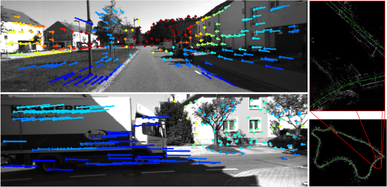
Figure 1: Self-Supervised 3D Keypoints for Robust Visual-Odometry. Left: The illustration shows the proposed self-supervised 3D keypoints learned purely from unlabeled monocular videos together with matched sparse 3D scene flow. Our method can effectively handle dynamic objects via outlier rejection thanks to structured pose estimation with our 3D keypoints. Right: The proposed 3D keypoint estimator is integrated into a state-of-the-art visual tracking framework for accurate, scale-aware, long-range monocular visual odometry.

Our main contribution is a fully self-supervised framework for the learning of depth-aware keypoint detection and description purely from unlabeled videos. Our novel formulation allows us to simultaneously learn keypoint detection, matching, and 3D lifting for robust visual ego-motion. Our second contribution lies in our principled use of the Orthogonal Procrustes algorithm to differentially regress an SE3 pose that is tightly coupled with the joint estimation of depth and keypoints from videos. We show that by enforcing strong regularization in the form of sparse multi-view geometric constraints, the keypoint and depth networks strongly benefit from joint optimization in an end-to-end framework. Finally, in our third contribution, we show results comparable to state-of-the-art stereo long-term tracking by integrating our self-supervised, monocular and depth-aware keypoints into existing visual tracking frameworks such as Direct Sparse Odometry (DSO) [13].

2 Related Work

Learning-based Methods for Keypoint Estimation. Over the past two decades, handcrafted image features such as SIFT [3] and ORB [4] have been the key enabler of visual SLAM [2] and SfM applications [1]. More recently, learning-based keypoint detectors and descriptors have advanced the state-of-the-art performance on challenging benchmarks. While generating ground truth data is a tedious and expensive process, DeTone et al. [9] has shown that synthetic data can be used for supervising keypoints which can be transferred to real world scenes. Alternatively, SfM [14] or two-view consistency [15, 16] can been used for keypoint learning without any additional labels. Single images have also been successfully used to train generalizable keypoints, with explicit descriptor losses by Christiansen et al. [10] or without by Tang et al. [17] . Additionally, descriptor discriminativeness can be learned, thus identifying high confidence matching regions [11]. Keypoints can also be learned in an end-to-end optimization for downstream tasks such as localization [18], relative pose estimation [12, 19] and 3D matching [20]. Our work extends previous work [10, 17] by combining self-supervised keypoint learning with depth estimation in monocular videos and by using the temporal consistency and scene geometry to regress a robust and repeatable keypoint estimator.

Learning-based Methods for Visual Odometry. While many learning-based methods exist, we will focus our discussion on self-supervised methods. Recently, Godard et al. [21] used stereo imagery to derive a photometric loss as proxy supervision to self-supervise a monocular depth network. This was extended to the generalized multi-view case by Zhou et al. [22], leveraging SfM constraints to simultaneously learn depth and camera ego-motion from monocular image sequences. A number of end-to-end self-supervised methods have been proposed, using super-resolution [23], learned [24] or self-discovered object detectors [25], two-stream rgb and depth networks [26], optical flow [27, 28, 29], modeling camera intrinsics [30], using adversarial networks [31], etc. Additionally, a number of hybrid methods have been proposed that combine self-supervised learning of the depth network with traditional methods, for example using a robust estimator to compute the fundamental matrix and eliminate outliers [28, 29] or by integrating learning [32, 33] with a state-of-the-art tracking method [13]. Similar to Zhan et al. [28], Zhao et al. [29], we use traditional methods to take advantage of the model-based PnP solution and the inliers established to outfit a differentiable pose estimation module within the self-supervised 3D keypoint learning framework. Differentiable Procrustes for point cloud alignment has been used previously by Wang and Solomon [34], Choy et al. [35], with a focus on global registration as a supervised learning problem. In [36] RGB-D data is registered through differentiable nonlinear least squares, allowing gradient flow and enabling end-to-end differentiable SLAM. In this paper we instead focus on self-supervised sparse keypoint detection and optimization for the task of ego-motion estimation, and show that our appearance-based depth-aware keypoints achieve superior results compared to other learning-based methods.

3 Self-Supervised Depth-Aware Keypoint Learning

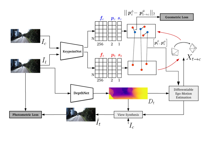
Figure 2: Monocular SfM-based 3D Keypoint Learning. We jointly optimize depth and keypoint networks thanks to differentiable view synthesis and geometric pose estimation modules. The whole system is self-supervised by strong geometric constraints on ego-motion thanks to our 3D keypoints.

Inspired by the concept of leveraging known geometric transformations to self-supervise and boost keypoint learning (DeTone et al. [9]), we propose a novel self-supervised method that relies on epipolar constraints in two-view camera geometry for robust 3D keypoint learning. Crucially, we generalize previous work by Tang et al. [17], Christiansen et al. [10] and self-supervise 3D keypoint learning to leverage the structured geometry of scenes in unlabeled monocular videos, without any need for supervision in the form of ground-truth or pseudo-ground-truth labels. Thanks to learning the 2D-to-3D keypoint lifting function from monocular videos, we can accurately estimate the ego-motion between temporally adjacent images (see Figure 2 for an overview of the proposed pipeline).

3.1 Notation

Our method works on sequences of monocular images, and we refer to $I_{t}$ as the target image and $I_{C}$ as the set of temporally adjacent context images, with $I_{c}\in I_{C}$. We jointly learn two networks. First the KeypointNet  $f_{k}:I\to\left(\bm{p},\bm{f},\bm{s}\right)$ regresses $N$ image keypoints consisting of positions $\bm{p}\in\mathbb{R}^{2\times N}$, descriptors $\bm{f}\in\mathbb{R}^{256\times N}$ and scores $\bm{s}\in\mathbb{R}^{N}$. Second, the DepthNet  $f_{D}:I\to D$ predicts the scale-ambiguous dense depth map $D$. We use $\bm{d}=D(\bm{p})\in\mathbb{R}^{N}$ to denote the values of $D$ associated with the keypoint positions $\bm{p}=[\bm{u},\bm{v}]^{T}$. The ego-motion estimator  $f_{x}(I_{c},I_{t})=X_{t\to c}=\begin{pmatrix}R&t\\ 0&1\end{pmatrix}\in\mathbb{SE}(3)$ predicts the relative 6-DoF rigid-body transformation between the target and context image. Throughout this manuscript, we use $\bm{p}$ to refer to sets of keypoints, while $p$ is used to refer to a single keypoint. Given two sets of detected keypoints, we define $\phi\left(\bm{f}_{t},\bm{f}_{c}\right)$ as the keypoint matching function that computes keypoint correspondences via reciprocal matching in descriptor space:

$$\begin{gathered}\phi\left(\bm{f}_{t},\bm{f}_{c}\right)=\{\left(f_{i},f_{j}\right)|\operatorname*{arg\,min}_{j^{\prime}}{\|f^{2}_{i}-f^{2}_{j^{\prime}}\|_{2}}=j\land\operatorname*{arg\,min}_{i^{\prime}}{\|f^{2}_{i^{\prime}}-f^{2}_{j}\|_{2}}=i\}\end{gathered}$$ (1)

with $f_{i}\in\bm{f}_{t}$ and $f_{j}\in\bm{f}_{c}$. $\phi$ defines an association between the keypoint positions in the two images, which we denote by $\left[\bm{p}^{\phi}_{t},\bm{p}^{\phi}_{c}\right]$. We use the correspondences $\left[\bm{p}^{\phi}_{t},\bm{p}^{\phi}_{c}\right]$ and their corresponding predicted depths $\left[\bm{d}^{\phi}_{t},\bm{d}^{\phi}_{c}\right]$ to estimate the rigid-body transformation $X_{t\to c}$ as described in detail in Section 3.2. Through $X_{t\to c}$, we define a joint optimization framework described in Section 3.3.

3.2 Differentiable Pose Estimation from Depth-Aware Keypoints

Pose Estimation via Perspective-n-Point. Using the estimated dense depth $D_{t}$ of the target image, we can compute the set $\bm{P}^{\phi}_{t}$ of 3D lifted keypoints through the operation: $\bm{P}^{\phi}_{t}=\pi^{-1}(\bm{p}^{\phi}_{t},\bm{d}^{\phi}_{t})$ where $\bm{P}_{t}=[\bm{X},\bm{Y},\bm{Z}]^{T}\in\mathbb{R}^{3\times N}$ and $\pi(\cdot)$ is the standard pinhole camera projection model. Using the keypoint correspondences $\left[\bm{p}^{\phi}_{t},\bm{p}^{\phi}_{c}\right]$, we then have a 3D-2D correspondence set and can use the PnP algorithm [37] to compute the initial relative pose transformation $X^{0}_{t\to c}=\begin{pmatrix}R_{0}&t_{0}\\ 0&1\end{pmatrix}$ to geometrically match the keypoints in the target image to those in the context image. Specifically, we minimize:

$$E_{\psi}(X^{0}_{t\to c})=\left\lVert\bm{p}^{\phi}_{c}-\pi\left(X^{0}_{t\to c}\cdot\bm{P}^{\phi}_{t}\right)\right\rVert_{2}~{}.$$ (2)

The estimated relative pose $X^{0}_{t\to c}$ is obtained by minimizing the residual error in Equation (2) using the Gauss-Newton (GN) method with RANSAC to ensure robustness to outliers (see Appendix F for details regarding this operation). This step allows us to compute the pose robustly, and yields an inlier set of correspondences $\left[\bm{p}^{\psi}_{t},\bm{p}^{\psi}_{c}\right]$. However, this procedure is not differentiable with respect to the keypoint set used to estimate it.

Residual Pose Correction via Orthogonal Procrustes. To alleviate the limitation of traditional PnP and allow end-to-end learning, we show how the initial pose estimate can be used to derive a 3D loss based on 3D-3D correspondences. We note that Sheffer and Wiesel [38] have recently proposed a differentiable version of the traditional PnP algorithm which combines deep learning with a model-based fine-tuning step. While this method has shown good results when trained with noisy correspondences, we follow instead the monocular direct method of Engel et al. [13] that performs frame-to-keyframe tracking. Specifically, we lift the context keypoints $\bm{p}^{\psi}_{c}$ to 3D using the re-projected depth of the source keypoints via the initial pose estimate $X^{0}_{t\to c}$. This allows us to form a 3D residual that can be used to recover the pose in closed-form (for convenience we omit the $\psi$ superscript below):

$$\begin{gathered}E_{OP}(X_{t\to c})={\|\bm{P}_{c}-X_{t\to c}\cdot\bm{P}_{t}\|}_{2}~{},\\ \text{where}~{}\mathbf{P}_{t}=\pi^{-1}(\bm{p}_{t},D_{t}(\bm{p}_{t}))~{},~{}\bm{P}_{c}=\pi^{-1}(\bm{p}_{c},\bm{d}_{c})~{},~{}\text{and}~{}\bm{d}_{c}=\left[X^{0}_{t\to c}\cdot\bm{P}_{t}\right]_{z}~{}.\\ \end{gathered}$$ (3)

The 3D residual above can be effectively minimized by estimating the rotation and translation separately using a closed-form solution on the established inlier set. We first estimate the rotation by subtracting the means of the points and minimizing Eq. 4 by solving an SVD in closed-form (otherwise known as the Orthogonal Procrustes problem [39]):

$$E(R)=\|\bm{P}^{*}_{c}-R\cdot\bm{P}^{*}_{t}\|_{2}~{},\quad\text{where}\enskip~{}\bm{P}^{*}_{i}=\bm{P}_{i}-\bm{\overline{P}}_{i}~{},$$ (4)

$$U\Sigma V=\mathtt{SVD}\left(\sum{(\bm{P}^{*}_{c})}^{T}(\bm{P}^{*}_{t})\right)~{},\enskip\text{where}\quad R=VU^{T}~{}.$$ (5)

Once the rotation $R$ is computed, the translation $t$ can be directly recovered by minimizing $t=\bm{P}^{*}_{c}-R\bm{\cdot}\bm{P}^{*}_{t}~{}$. Thus, the gradients for the pose rotation and translation can be effectively propagated with respect to the lifted 3D keypoint locations, making the overall pose estimation fully-differentiable. The differentiable pose estimated using the 2D keypoints from the source image and 3D keypoints from the target image tightly couples keypoint and depth estimation, thereby allowing both predictions to be further optimized using the overall keypoint learning objective described next.

3.3 Joint Self-Supervised Learning of Depth and Keypoints

We self-supervise the joint end-to-end learning of the keypoint and depth networks using a combination of a geometric keypoint loss $\mathcal{L}_{kpn}$, based on keypoint reprojection error, and a dense photometric loss $\mathcal{L}_{depth}$, based on the warped projection of $D_{t}$ in $I_{c}$: $\mathcal{L}=\mathcal{L}_{depth}+\alpha\mathcal{L}_{kpn}$.

3.3.1 Keypoint Loss

The total keypoint loss is composed of three terms: $\mathcal{L}_{kpn}=\mathcal{L}_{geom}+\beta_{1}\mathcal{L}_{desc}+\beta_{2}\mathcal{L}_{score}$.

Geometric Loss.  Using $X_{t\to c}$ and $\bm{P}^{\phi}_{t}$, we compute the warped keypoints from image $I_{t}$ to $I_{c}$ as:

$$\begin{gathered}\mathbf{p}^{\phi}_{t\to c}=\pi\left(X_{t\to c}\bm{P}^{\phi}_{t}\right)=\pi(R\cdot\bm{P}^{\phi}_{t}+t)\end{gathered}$$ (6)

At training time, we aim to minimize the distance between the set of warped keypoints $\bm{p}^{\phi}_{t\to c}$ and the set of corresponding keypoints $\bm{p}^{\phi}_{c}$ obtained via descriptor matching (Eq. 1):

$$\begin{gathered}\mathcal{L}_{geom}=||\bm{p}^{\phi}_{c}-\bm{p}^{\phi}_{t\to c}||_{2}\end{gathered}$$ (7)

Descriptor Loss.  Following Tang et al. [17], we use nested hardest sample mining to self-supervise the keypoint descriptors between the two views. Given anchor descriptors $\bm{f}_{t}$ from the target frame and their associated positive descriptors $\bm{f}_{+}=\bm{f}^{\phi}_{t}$ in the source frame, we define the triplet loss:

$$\begin{gathered}\mathcal{L}_{desc}=\max(0,\|\bm{f},\bm{f}_{+}\|_{2}-\|\bm{f},\bm{f}_{-}\|_{2}+m)~{},\end{gathered}$$ (8)

where $\bm{f}_{-}$ is the hardest descriptor sample mined from $\bm{f}_{s}$ with margin $m$.

Score Loss.  The score loss is introduced to identify reliable and repeatable keypoints in the matching process. In particular, we want to ensure that (i) the feature-pairs have consistent scores across matching views; and (ii) the network learns to predict high scores for good keypoints with low geometric error and strong repeatability. Following Christiansen et al. [10], we achieve this by minimizing the squared distance between scores for each matched keypoint-pair, and minimizing (respectively maximizing) the average score of a matched keypoint-pair if the distance between the paired keypoints is greater (respectively smaller) than the average distance:

$$\begin{gathered}\mathcal{L}_{score}=\left[\frac{(\bm{s}^{\phi}_{t}+\bm{s}^{\phi}_{c})}{2}\cdot(\|(\bm{p}^{\phi}_{t\to c},\bm{p}^{\phi}_{c}\|_{2}-\bar{\bm{d}})+(\bm{s}^{\phi}_{t}-\bm{s}^{\phi}_{c})^{2}\right]~{},\end{gathered}$$ (9)

where $\bm{s}^{\phi}_{t}$ and $\bm{s}^{\phi}_{c}$ are the scores of the target and context keypoints respectively, and $\bar{\bm{d}}$ is the average reprojection error of corresponding keypoints given by $\bar{\bm{d}}=\sum_{i}^{L}\frac{\|\left(p^{\phi}_{i\to c}\right)^{2}-\left(p^{\phi}_{i}\right)^{2}\|_{2}}{L}$, and $L$ denotes the total number of keypoint pairs.

3.3.2 Depth Loss

The total depth loss is also composed of three terms: $\mathcal{L}_{depth}=\mathcal{L}_{photo}+\beta_{3}\mathcal{L}_{smooth}+\beta_{4}\mathcal{L}_{const}$.

Photometric loss. Following [22, 40, 41], we warp the estimated dense depth of the target image $D_{t}$ via the predicted ego-motion estimate $X_{t\to c}$ to the context frame $I_{c}$. Using [42], we synthesize $\hat{I}_{t}=I_{c}\left(q_{t\to c}\right)$ for all pixels $q_{t}\in I_{t}$, where $q_{t\to c}$ is the context pixel computed by warping the target pixel $q_{t}$ via Equation 6. This operation is done via grid sampling with bilinear interpolation [42] and thus is differentiable. Following [22, 40, 42], we impose a dense photometric loss which consists of a structural similarity (SSIM) loss [43] (defined in Appendix E) and an L1 pixel-wise loss term:

$$\begin{gathered}\mathcal{L}_{photo}\left(I_{t},\hat{I_{t}}\right)=\gamma~{}\frac{1-\text{SSIM}\left(I_{t},\hat{I_{t}}\right)}{2}+\left(1-\gamma\right)~{}|I_{t}-\hat{I_{t}}|~{}.\end{gathered}$$ (10)

In addition, we mask out static pixels which have a warped photometric loss $\mathcal{L}_{photo}(I_{t},\hat{I}_{t})$ higher than their corresponding unwarped photometric loss $\mathcal{L}_{photo}(I_{t},I_{c})$, calculated using the original source image without view-synthesis as described in [40]. Additionally, we employ a smoothness loss term $\mathcal{L}_{smooth}$ following [21] which we describe in detail in Appendix E.

Depth Consistency.  While recovering scale-consistent depth is not a strict requirement for the proposed framework to learn 3D keypoints, scale-consistency is important for tasks that involve accurate ego-motion estimation [25, 30]. To this end, we incorporate a depth consistency term that discourages scale-drift between dense depth predictions in adjacent frames:

$$\begin{gathered}\mathcal{L}_{const}=\frac{\|D_{t}(\bm{p}^{\phi}_{t})-D_{c}(\bm{p}^{\phi}_{c})\|}{D_{t}(\bm{p}^{\phi}_{t})+D_{c}(\bm{p}^{\phi}_{t})}\end{gathered}$$ (11)

Note that $\mathcal{L}_{const}$ is a sparse loss defined based on the correspondences $\left[\mathbf{p}^{\phi}_{t},\mathbf{p}^{\phi}_{c}\right]$.

4 Experiments

We evaluate our system on the KITTI [44] dataset and report $t_{rel}$ - average translational RMSE drift (%) on trajectories of length 100-800m, and $r_{rel}$ - average rotational RMSE drift (deg /100m) on trajectories of length 100-800m. All our $t_{rel}$ results are obtained after performing a single Sim(3) alignment step [45] w.r.t. the ground truth trajectories. We report results for the two main protocols used in related works. Most end-to-end learning based methods train on the KITTI sequences 00-08 and evaluate on seq. 09 and 10. These results are summarized in Table 2, with more details in Appendices G and I. A number of methods including DVSO [32] and D3VO [33] train on the Eigen [46] train split, which includes sequences 01, 02, 06, 08, 09 and 10; in this case the test sequences are 00, 03, 04, 05 and 07. We summarize our results for this protocol in Table 1. Additionally, we report in the standard depth evaluation metrics on the Eigen [46] test split in Appendix C.

To evaluate the performance of our kepoint detector and decriptor we use the HPatches [47] dataset, which contains a set of 116 image sequences (illumination and viewpoint) for a total of 580 image pairs. We quantify detector performance through the Repeatability and Localization Error metrics and descriptor performance through the Correctness and Matching Score metrics (the exact definition of these metrics can be found in Appendix J). For a fair comparison, we evaluate the results generated without applying Non-Maxima Suppression (NMS). Following related work [17, 10, 9], we pre-train our KeypointNet on the COCO [48] dataset, which contains $118k$ training images. We note that pretraining on COCO is self-supervised, as described in Sec. 4.1.

4.1 Training

We implement our networks in PyTorch [49] using the ADAM optimizer [50]. We use $10^{-4}$ as the learning rate and train KeypointNet and DepthNet jointly for $50$ epochs with a batch size of $8$. We implement KeypointNet following [17], with the mention that we use an ImageNet pre-trained ResNet-18 backbone, which we find performs better than the reference architecture. We follow [40] and implement DepthNet using an ImageNet [51] pretrained ResNet-18 backbone along with a depth decoder that outputs inverse depth at 4 different resolution scales. However, at test-time, only the highest resolution scale is used for 2D-to-3D keypoint lifting. We describe our networks in detail in Appendix A. We train on snippets of 3 images $\left(I_{t-\Delta t},I_{t},I_{t+\Delta t}\right)$, for $\Delta t\in[1,2,4]$ with target image $I_{t}$ and images $\left(I_{t-\Delta t},I_{t+\Delta t}\right)\in I_{C}$ as context images. Using the pair of target and context images we compute the losses as defined in Section 3.3. The dense photometric loss is computed over the context $I_{C}$ as shown in Equation 10. In all our experiments we set $\alpha=0.1$, $\beta_{1}=\beta_{2}=1.0$, $\beta_{3}=\beta_{4}=0.1$, and $\gamma=0.85$. Additionally, starting from the target image $I_{t}$, we also perform Homography Adaptation similar to [17], e.g., translation, rotation, scaling, cropping and symmetric perspective transform and we apply per-pixel Gaussian noise, color jitter, and Gaussian blur to the images. Our method runs at 30fps on images of resolution 640x192 on a V100 GPU.

Pretrained baseline. We pretrain KeypointNet on COCO using Homography Adaptation for $50$ epochs using a learning rate of $5\cdot 10^{-4}$ which is halved after $40$ epochs. We refer to this as our baseline KeypointNet, and evaluate its performance in Table 4. To speed up convergence, we pretrain our DepthNet on the KITTI training sequences using the method described in [40]. We train for 200 epochs with a learning rate of $10^{-4}$ which is decayed by $0.5$ every $40$ epochs. We refer to this as our baseline DepthNet, and we evaluate its performance in the ablative evaluations in Table 3.

4.2 Direct Sparse Odometry (DSO) Integration

To evaluate tracking performance, we integrate our self-supervised, depth-aware keypoints into the DSO framework of Engel et al. [13], and we show that we are able to achieve long-term tracking results which are especially on par with stereo methods such as DVSO [32] or ORB-SLAM2 [52]. Unlike other monocular visual odometry approaches, the superior keypoint matching and stable 3D lifting performance of our proposed method allows us to bootstrap the tracking system, rejecting false matches and outliers and avoiding significant scale-drift. Our integration is built on top of the windowed sparse direct bundle adjustment formulation of DSO. Specifically, we improve depth-initialization of keyframes in the original DSO implmenetation by using the depth estimated through our proposed self-supervised 3D keypoints. In addition, we modify the hand-engineered direct semi-dense tracking component to use the proposed sparse and robust learned keypoint-based method introduced in this work. We describe the DSO integration in more details in Appendix D.

4.3 Visual Odometry Performance

Method	Type	01	02	06	08	09	10	00	03	04	05	07	Train	Test
	$t_{rel}$ - Average Translational RMSE drift (%) on trajectories of length 100-800m.
Mono-DSO [53]	Mono	9.17	114	42.2	177	28.1	24.0	-	-	-	-	-	65.75	-
ORB-SLAM-M [52]	Mono	-	-	-	32.40	-	-	25.29	-	-	26.01	24.53	-	27.05
Ambrus et al [26]	Mono	17.59	6.82	8.93	8.38	6.49	9.83	7.16	7.66	3.8	6.6	11.48	9.67	7.34
UnDeepVO [54]	Stereo	69.1	5.58	6.20	4.08	7.01	10.6	4.14	5.00	4.49	3.40	3.15	11.68	8.81
SuperDepth [23]	Stereo	13.48	3.48	1.81	2.25	3.74	2.26	6.12	7.90	11.80	4.58	7.60	4.50	7.60
DVSO [32]	Stereo	1.18	0.84	0.71	1.03	0.83	0.74	0.71	0.77	0.35	0.58	0.73	0.89	0.63
D3VO [33]	Stereo	1.07	0.80	0.67	0.78	0.62	-	-	-	-	-	-	-	0.82
Ours	Mono	17.79	3.15	1.88	3.06	2.69	5.12	2.76	3.02	1.93	3.30	2.41	5.61	2.68
Ours + DSO	Mono	4.70	3.62	0.92	2.46	2.31	5.24	1.83	1.21	0.76	1.84	0.54	3.21	1.24
	$r_{rel}$ - Average Rotational RMSE drift (${}^{{\circ}}/100m$) on trajectories of length 100-800m.
ORB-SLAM-M [52]	Mono	-	-	-	12.13	-	-	7.37	-	-	10.62	10.83	-	10.23
Ambrus et al [26]	Mono	1.01	0.87	0.39	0.61	0.86	0.98	1.70	3.49	0.42	0.90	2.05	0.79	1.71
UnDeepVO [54]	Stereo	1.60	2.44	1.98	1.79	3.61	4.65	1.92	6.17	2.13	1.5	2.48	2.45	4.13
SuperDepth [23]	Stereo	1.97	1.10	0.78	0.84	1.19	1.03	2.72	4.30	1.90	1.67	5.17	1.15	3.15
DVSO [32]	Stereo	0.11	0.22	0.20	0.25	0.21	0.21	0.24	0.18	0.06	0.22	0.35	0.20	0.21
Ours	Mono	0.72	1.01	0.80	0.76	0.61	1.07	1.17	2.45	1.93	1.11	1.16	0.83	1.56
Ours + DSO	Mono	0.16	0.22	0.13	0.31	0.30	0.29	0.33	0.33	0.18	0.22	0.23	0.24	0.26

Table 1: Comparison of vision-based trajectory estimation with state-of-the-art methods. The Type column indicates the data used at training time. Note: All methods are evaluated on monocular data. Bold text denotes the best method trained on monocular data; _ denotes the best overall method. Training seq. 01, 02, 06, 08, 09 and 10; test seq. 00, 03, 04, 05 and 07. The numbers for [52] are reported from [54]; the numbers for [53] are reported from [33].

We summarize our visual odometry results and comparisons with state-of-the-art methods in Table 1, and we note that our method outperforms all other monocular-trained methods, particularly in the $t_{rel}$ metric. For $r_{rel}$ we note that [26] achieves better results on some sequences, which we attribute to difficulty in matching keypoints in those settings, however our $r_{rel}$ is superior on average over the test sequences. Our method also outperforms stereo-trained methods except for DVSO [32] and D3VO [33]. However, we emphasize that while both [32, 33] are trained from a wide-baseline stereo setup which provides a strong prior for outlier rejection, our system is trained in a self-supervised manner purely relying on monocular videos - a significantly harder problem. The results indicate that when integrated with tracking frameworks such as DSO our depth-aware keypoints provide superior matching performance that even rivals state-of-the-art methods trained on stereo imagery.

	Bian et al [25]	EPC++ [27]	Monodepth2$\ddagger$ [40]	DF-VO [28] PnP	Zhao et al [29]	SGANVO [31]	Gordon et al [30]	DF-VO [28]	Ours
	$t_{rel}$ - Average Translational RMSE drift (%) on trajectories of length 100-800m.
Seq 09	11.2	8.84	5.28	7.12	6.93	4.95	2.7	2.47	3.14
Seq 10	10.1	8.86	8.47	6.83	4.66	5.89	6.8	1.96	5.45
Mean	10.7	8.85	7.14	6.98	5.76	5.42	4.75	2.21	4.30
	$r_{rel}$ - Average Rotational RMSE drift (${}^{{\circ}}/100m$) on trajectories of length 100-800m.
Seq 09	3.35	3.34	1.60	2.43	0.44	2.37	-	0.30	0.73
Seq 10	4.96	3.18	2.26	3.88	0.62	3.56	-	0.31	1.18
Mean	4.20	3.26	1.73	3.12	0.53	3.02	-	0.31	0.90

Table 2: Comparison of vision-based trajectory estimation with state-of-the-art monocular methods. Bold text denotes the best performing method; _ denotes the second best method. Training seq. 00-08; test seq: 09 and 10. $\ddagger$ - the numbers of [40] are based on our own implementation.

Additionally, we report our results when training on KITTI sequences 00-08 in Table 2. We note that our method outperforms all other monocular methods except for DF-VO [28] and [29] for $r_{rel}$. Both [29, 28] heavily rely on optical-flow and RANSAC-based essential/fundamental matrix computation and scale-factor recovery. Recall that our method uses PnP (as described in Section 3.2) for pose estimation. When comparing with the PnP-based version DF-VO [28] (DF-VO PnP in Table 2), we observe that our method performs much better, which we attribute to the direct optimization of sparse 2D-3D keypoints, as opposed to [28] which relies purely on dense optical flow. Finally, we record that our method performs worse on sequence 01 compared to the other sequences. In this sequence the vehicle is driving at high speeds on the highway and the image contains a high number of sky pixels, making this a challenging environment for feature detection and matching; we note that a number of other methods also perform poorly in this setting [26, 54, 23, 28].

4.4 Ablation Study

We summarize our ablative analysis in Table 3. Our baseline - KeypointNet pre-trained on COCO and DepthNet trained on KITTI, but the two are not optimized together - shows superior results compared to most monocular methods (see Tables 1 and 2), thus motivating our approach of combining keypoints and depth in a self-supervised learning framework. We notice a significant improvement when training the two networks together (Row 2: Ours $-$ Diff Pose). Adding the differential pose estimation (Row 5: Ours ) further improves the performance of our system for the $t_{rel}$ metric; we note that the $r_{rel}$ test metric does not improve, mostly due to an error in Sequence $04$ (please refer to Appendix G for detailed results). We further ablate the KeypointNet (Row 3: Ours $-$ KPN trained) - i.e., we estimate the ego-motion using the DepthNet after training together with the KeypointNet, but we use the original KeypointNet trained only on COCO. We perform a similar experiment ablating the trained DepthNet (Row 4: Ours $-$ DN trained). Finally, when integrated in DSO (Row 6: Ours DSO) our results improve significantly, which we attribute to the robustness of our features to scene appearance and geometry. We provide more details in Appendix G, and emphasize that all our experiments, including pretraining, are done in a self-supervised fashion, without any supervision.

	KPN	DN	KPN	DN	Diff	DSO	$r_{rel}$		$t_{rel}$
Method	baseline	baseline	trained	trained	Pose		train	test	train	test
1. Baseline	$\checkmark$	$\checkmark$	-	-	-	-	1.02	1.63	6.08	3.14
2. Ours $-$ Diff Pose	$\checkmark$	$\checkmark$	$\checkmark$	$\checkmark$	-	-	0.89	1.43	6.12	2.92
3. Ours $-$ KPN trained	$\checkmark$	$\checkmark$	-	$\checkmark$	$\checkmark$	-	0.93	1.61	5.94	2.88
4. Ours $-$ DN trained	$\checkmark$	$\checkmark$	$\checkmark$	-	$\checkmark$	-	0.91	1.58	5.38	2.88
5. Ours	$\checkmark$	$\checkmark$	$\checkmark$	$\checkmark$	$\checkmark$	-	0.83	1.56	5.61	2.68
6. Ours + DSO	$\checkmark$	$\checkmark$	$\checkmark$	$\checkmark$	$\checkmark$	$\checkmark$	0.24	0.26	3.21	1.24

Table 3: Ablative analysis: Diff Pose - the differentiable pose component (Section 3.2), KPN trained - the trained version of the KeyPointNet (i.e., using only the baseline), DN trained - the trained version of the DepthNet. Training seq. 01, 02, 06, 08, 09, 10; test seq. 00, 03, 04, 05, 07.

4.5 Keypoint Detector and Descriptor Performance

Table 4 shows the performance of our method on HPatches [47]. We note that by improving the network capacity and using a ResNet-18 architecture, our baseline outperforms all classical as well as learning-based methods (recall that our KeypointNet baseline is trained only on COCO, and can thus be directly compared to these methods). Further, we note similar metrics between our baseline method and our method after training on KITTI (KeypointNet baseline vs KeypointNet). We conclude that by training with the proposed losses in a joint self-supervised framework, our keypoints have gained geometric understanding and can be used for state-of-the-art ego-motion estimation while at the same time retaining their robustness to illumination and viewpoint changes.

Method	240x320, 300 points						480 x 640, 1000 points
	Rep.	Loc.	Cor-1	Cor-3	Cor-5	M.Score	Rep.	Loc.	Cor-1	Cor-3	Cor-5	M.Score
ORB [4]	0.532	1.429	0.131	0.422	0.540	0.218	0.525	1.430	0.286	0.607	0.71	0.204
SURF [55]	0.491	1.150	0.397	0.702	0.762	0.255	0.468	1.244	0.421	0.745	0.812	0.230
BRISK [56]	0.566	1.077	0.414	0.767	0.826	0.258	0.746	0.211	0.505	1.207	0.300	0.653
SIFT [3]	0.451	0.855	0.622	0.845	0.878	0.304	0.421	1.011	0.602	0.833	0.876	0.265
LF-Net(indoor) [15]	0.486	1.341	0.183	0.628	0.779	0.326	0.467	1.385	0.231	0.679	0.803	0.287
LF-Net(outdoor) [15]	0.538	1.084	0.347	0.728	0.831	0.296	0.523	1.183	0.400	0.745	0.834	0.241
SuperPoint [9]	0.631	1.109	0.491	0.833	0.893	0.318	0.593	1.212	0.509	0.834	0.900	0.281
UnsuperPoint [10]	0.645	0.832	0.579	0.855	0.903	0.424	0.612	0.991	0.493	0.843	0.905	0.383
IO-Net [17]	0.686	0.890	0.591	0.867	0.912	0.544	0.684	0.970	0.564	0.851	0.907	0.510
KeypointNet Baseline	0.683	0.816	0.624	0.879	0.924	0.573	0.682	0.898	0.581	0.848	0.913	0.534
KeypointNet	0.686	0.799	0.532	0.858	0.906	0.578	0.674	0.886	0.529	0.867	0.920	0.529

Table 4: Keypoint and descriptor performance on HPatches [47]. Repeatability and Localization Error measure keypoint performance while Correctness (pixel threshold 3) and Matching score measure descriptor performance. Higher is better for all metrics except Localization Error.

5 Conclusion

In this paper, we proposed a fully self-supervised framework for depth-aware keypoint learning from unlabeled monocular videos by incorporating a novel differentiable pose estimation module that simultaneously optimizes the keypoints and their depths in a Structure-from-Motion setting. Unlike existing learned keypoint methods that employ only homography adaptation, we exploit the temporal context in videos to further boost the repeatability and matching performance of our proposed keypoint network. The resulting 3D keypoints and associated descriptors exhibit superior performance compared to all other traditional and learned methods, and are also able to learn from realistic non-planar 3D scenes. Finally, we show how our proposed network can be integrated with a monocular visual odometry system to achieve accurate, scale-aware, long-term tracking results that are on par with state-of-the-art stereo-methods.

Appendix A Architecture Diagram

ResNet18-DepthNet. we provide a detailed description of our DepthNet architecture in Table 5. Note that we follow Godard et al. [21] and use a ResNet18 encoder followed by a decoder which outputs inverse depth at 4 scales.

	Layer Description	K	Output Tensor Dim.
#0	Input RGB image		3$\times$H$\times$W
ResidualBlock
	Conv2d + BatchNorm + ReLU	3
	Conv2d + BatchNorm	3
Depth Encoder
#1	Conv2d (S2) + BatchNorm + ReLU	7	64$\times$H/2$\times$W/2
#2	Conv2d + BatchNorm + ReLU	3	64$\times$H/2$\times$W/2
#3	ResidualBlock (#2) x2	-	64$\times$H/2$\times$W/2
#4	Max. Pooling ($\times$1/2)	3	64$\times$H/4$\times$W/4
#5	ResidualBlock (#3 + $2) x2	-	128$\times$H/4$\times$W/4
#6	Max. Pooling ($\times$1/2)	3	128$\times$H/8$\times$W/8
#7	ResidualBlock (#4 + #3) x2	-	256$\times$H/8$\times$W/8
#8	Max. Pooling ($\times$1/2)	3	256$\times$H/16$\times$W/16
#9	ResidualBlock (#5 + #4) x2	-	512$\times$H/16$\times$W/16
Depth Decoder
#10	Conv2D + ELU (#9)	3	128$\times$H/16$\times$W/16
#11	Conv2D + Upsample (#10)	3	128$\times$H/8$\times$W/8
#12	Conv2D + Sigmoid	3	1$\times$H/8$\times$W/8
#13	Conv2D + ELU	3	64$\times$H/8$\times$W/8
#14	Conv2D + Upsample(#7 $\oplus$ #13)	3	64$\times$H/4$\times$W/4
#15	Conv2D + Sigmoid	3	1$\times$H/8$\times$W/8
#16	Conv2D + ELU	3	32$\times$H/4$\times$W/4
#17	Conv2D + Upsample (#5 $\oplus$ #16)	3	32$\times$H/2$\times$W/2
#18	Conv2D + Sigmoid	3	1$\times$H/8$\times$W/8
#19	Conv2D + ELU	3	16$\times$H/2$\times$W/2
#20	Conv2D + Upsample (#3 $\oplus$ #19)	3	16$\times$H$\times$W
#21	Conv2D + Sigmoid	3	1$\times$H$\times$W

Table 5: DepthNet diagram. Line numbers in bold indicate output inverse depth layer scales. Upsample is a nearest-neighbor interpolation operation that doubles the spatial dimensions of the input tensor. $\oplus$ denotes feature concatenation for skip connections.

ResNet18 KeypointNet. Table 6 details the network architecture of our KeypointNet. We follow [17] but change the network encoder and use a ResNet18 architecture instead, which we found to perform better.

	Layer Description	K	Output Tensor Dim.
#0	Input RGB image		3$\times$H$\times$W
ResidualBlock
	Conv2d + BatchNorm + ReLU	3
	Conv2d + BatchNorm	3
KeyPoint Encoder
#1	Conv2d (S2) + BatchNorm + ReLU	7	64$\times$H/2$\times$W/2
#2	Conv2d + BatchNorm + ReLU	3	64$\times$H/2$\times$W/2
#3	ResidualBlock (#2) x2	-	64$\times$H/2$\times$W/2
#4	Max. Pooling ($\times$1/2)	3	64$\times$H/4$\times$W/4
#5	ResidualBlock (#3 + $2) x2	-	128$\times$H/4$\times$W/4
#6	Max. Pooling ($\times$1/2)	3	128$\times$H/8$\times$W/8
#7	ResidualBlock (#4 + #3) x2	-	256$\times$H/8$\times$W/8
#8	Max. Pooling ($\times$1/2)	3	256$\times$H/16$\times$W/16
#9	ResidualBlock (#5 + #4) x2	-	512$\times$H/16$\times$W/16
KeyPoint Decoder
#10	Conv2D + BatchNorm + LReLU (#9)	3	256$\times$H/16$\times$W/16
#11	Conv2D + Upsample (#10)	3	256$\times$H/8$\times$W/8
#12	Conv2D + BatchNorm + LReLU	3	256$\times$H/8$\times$W/8
#13	Conv2D + Upsample(#7 $\oplus$ #12)	3	128$\times$H/4$\times$W/4
#14	Conv2D + BatchNorm + LReLU	3	128$\times$H/4$\times$W/4
#15	Conv2D + Upsample (#5 $\oplus$ #14)	3	64$\times$H/2$\times$W/2
#16	Conv2D + BatchNorm + LReLU	3	64$\times$H/2$\times$W/2
Score Head
#12	Conv2d + BatchNorm + LReLU (#12)	3	256$\times$H/8$\times$W/8
#13	Conv2d + Sigmoid	3	1$\times$H/8$\times$W/8
Location Head
#14	Conv2d + BatchNorm + LReLU (#12)	3	256$\times$H/8$\times$W/8
#15	Conv2d + Tan. Harmonic	3	2$\times$H/8$\times$W/8
Descriptor Head
#16	Conv2d + BatchNorm + LReLU (#16)	3	64$\times$H/2$\times$W/2
#17	Conv2d	3	64$\times$H/2$\times$W/2

Table 6: KeypointNet diagram. Upsample is a nearest-neighbor interpolation operation that doubles the spatial dimensions of the input tensor. $\oplus$ denotes feature concatenation for skip connections.

Appendix B Video

The accompanying video presents our contributions and demonstrates the long-term visual odometry accuracy obtained by our method on a video sequence. The main panel (top, center) shows our real-time semi-dense reconstruction along with the vehicle trajectory. The bottom panel shows (from left to right): the flow of inlier keypoints, color-coded based on depth; the estimated monocular depth; and finally, the number of matched keypoints versus the number tracked inliers.

Appendix C Dense Depth Evaluation

	Method	Abs Rel	Sq Rel	RMSE	RMSElog	$\delta<1.25$	$\delta<1.25^{2}$	$\delta<1.25^{3}$
	Monodepth2 [40]	0.090	0.545	3.942	0.137	0.914	0.983	0.995
	DepthNet baseline	0.089	0.543	3.968	0.136	0.916	0.982	0.995
	DepthNet finetuned	0.094	0.572	3.805	0.138	0.912	0.981	0.994

Table 7: Quantitative performance comparison of depth estimation on the KITTI dataset for reported depths of up to 80m. For Abs Rel, Sq Rel, RMSE and RMSE_log lower is better, and for $\delta<1.25$, $\delta<1.25^{2}$ and $\delta<1.25^{3}$ higher is better. All networks have been pre-trained on ImageNet [51]. We evaluate on the annotated KITTI depth maps from [57]. At test-time, the scale for all the methods is corrected using the median ground-truth depth from the LiDAR.

We perform a qualitative evaluation of our DepthNet on the KITTI dataset, specifically on the Eigen [46] test split, and report the numbers in Table 7. We also include the numbers reported by [40] and note that our DepthNet baseline numbers are on par with those of [40] (which correspond to row 1. Baseline of Table 3 in the main text). Table 7 also shows our numbers after fine-tuning the DepthNet and KeypointNet through the proposed Multi-View Adaptation method (which correspond to row 5. Ours of Table 3 in the main text). We note a slight decrease in the Abs Rel and Sq Rel metrics, but otherwise the numbers are within error margin with respect to our baseline. These results provide an important sanity check: as the main focus of this work is sparse, depth-aware keypoint learning, we don’t expect to see much variation when performing dense depth evaluation. We mention that sparsely evaluating the depth using the keypoints regressed by our method is not feasible using the depth available in the KITTI dataset: even using the denser depth maps provided by [57], only about $10\%$ of our keypoints have valid depths in the ground truth maps, which amounts to a very small number of points ($<50$) per image.

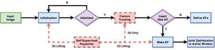
Figure 3: Direct Sparse Odometry (DSO) Integration. We leverage our self-supervised depth-aware keypoint detection and description to improve the depth initialization and robust feature tracking components. The red block and arrows show that where the 3D keypoint is affecting the original DSO system, the purple texts show where 2D and 3D information is utilized.

Appendix D Direct Sparse Odometry (DSO) Integration

In this section, we explain how the fully self-supervised depth-aware keypoint network can be incorporated as the front-end into a visual SLAM framework. We show that by integrating our method into a state-of-the-art monocular visual tracking framework such as DSO [13], we are able to achieve high accuracy long-term tracking results as reported in Table 1 of the main paper.

Unlike other monocular visual odometry approaches, the superior keypoint matching and stable 3D lifting performance of our proposed method allows us to bootstrap the tracking system, rejecting false matches and outliers and avoiding significant scale-drift.

Figure 3 shows the whole pipeline of our Deep Semi-Direct Sparse Odometry (DS-DSO) system, which is built on top of the windowed sparse direct bundle adjustment formulation of DSO. As illustrated, we improve depth-initialization of keyframes in the original DSO implmenetation by using the depth estimated through our proposed self-supervised 3D keypoint network. In addition, we modify the hand-engineered direct semi-dense tracking component to our proposed sparse and robust learned keypoint-based method introduced in this work.

Appendix E Depth losses

Depth Smoothness Loss.  In order to regularize the depth in texture-less low-image gradient regions, we use an edge-aware loss term similar to [21]:

$$\mathcal{L}_{smooth}=|\delta_{x}\hat{D}_{t}|e^{-|\delta_{x}I_{t}|}+|\delta_{y}\hat{D}_{t}|e^{-|\delta_{y}I_{t}|}~{}.$$ (12)

Structural Similarity (SSIM) loss. We define the SSIM loss [43] as:

$$SSIM(\mathbf{x},\mathbf{y})=\frac{(2\mu_{x}\mu_{y}+C_{1})(2\sigma_{xy}+C_{2})}{(\mu_{x}^{2}+\mu_{y}^{2}+C_{1})(\sigma_{x}^{2}+\sigma_{y}^{2}+C_{2})}~{},$$ (13)

with $C_{1}=1e^{-4}$ and $C_{2}=9e^{-4}$. To compute the per-patch mean and standard deviation $\mu_{x}$ and $\sigma_{x}$ we use a $3\times 3$ block filter.

Appendix F Pose Estimation

Recall that we aim to minimize:

$$E_{\psi}(X^{0}_{t\to c}) =\left\lVert\bm{p}^{\phi}_{c}-\pi\left(X^{0}_{t\to c}\cdot\bm{P}^{\phi}_{t}\right)\right\rVert_{2}$$ (14)

$$=\left\lVert\bm{p}^{\phi}_{c}-\pi\left(R\cdot\bm{P}^{\phi}_{t}+t\right)\right\rVert_{2}~{},$$ (15)

where $R\in\mathbb{R}^{3\times 3}$ is the rotation matrix and $t\in\mathbb{R}^{3}$ is the translation vector. They together compose a rigid body transform $\mathrm{exp}(\hat{x})\in\mathbb{SE}(3)$, which is defined by $x=[\omega^{T},t^{T}]^{T}\in\mathfrak{se}(3)$. $x$ is a member of the Lie algebra and is mapped to the Lie group $\mathbb{SE}(3)$ through the matrix exponential $\mathrm{exp}(.)$:

$$\begin{gathered}\mathrm{exp}({\hat{{x}}})=\begin{bmatrix}{R}&{t}\\ {0}&1\end{bmatrix}\quad,\quad{\hat{{x}}}=\begin{bmatrix}[{\omega}]_{\times}&{t}\\ {0}&1\end{bmatrix}\\ \end{gathered}~{},$$ (16)

where $[{\omega}]_{\times}$ is the skew-symmetric matrix of ${\omega}$.

The estimated relative pose can be obtained by optimizing the residual error in Equation (14). The Gauss-Newton (GN) method is used to solve this non-linear least-squares problem. GN calculates ${x}$ iteratively as follows:

$${x}^{(n+1)}={x}^{(n)}-\left(\mathbf{J_{r}}^{T}\mathbf{J_{r}}\right)^{-1}\mathbf{J_{r}}^{\mathbf{T}}\mathbf{r}({x}^{(n)})~{},$$ (17)

where $\mathbf{J_{r}}$ is the Jacobian matrix with respect to the residual measurements. RANSAC is performed to achieve a robust estimation and reject three major types of outliers which break the ego-motion assumption: false-positive matching pairs, dynamic objects or points with wrong depth estimations.

Appendix G Detailed Results for the Pose Ablation Study

Table 8 provides detailed results on all the KITTI odometry sequences for each entry of our ablation study (Table 3 of the main text). We note that (i) the proposed contributions - i.e. row 2 vs row 1 and row 5 vs row 1 consistently improve over the baseline; and that (ii) by swapping out the KeypointNet or DepthNet trained using the proposed method with their baseline counterparts (rows 3 and 4) results in worse performance for both the $t_{rel}$ and $r_{rel}$ metrics. Thus we conclude that the proposed training procedure along with the differentiable pose component improves both the DepthNet and KeypointNet for the task of Visual Odometry.

Method	Type	01∗	02∗	06∗	08∗	09∗	10∗	00†	03†	04†	05†	07†	Train	Test
	$t_{rel}$ - Average Translational RMSE drift (%) on trajectories of length 100-800m.
Baseline	Mono	18.96	3.35	2.16	3.80	3.15	5.06	3.50	3.64	2.33	3.25	3.00	6.08	3.14
Ours $-$ Diff Pose	Mono	20.17	3.37	2.15	3.01	2.61	5.39	2.89	3.10	2.88	3.09	2.66	6.12	2.92
Ours $-$ KPN trained	Mono	19.09	3.30	2.23	3.16	2.84	5.03	2.83	3.29	2.02	3.69	2.58	5.94	2.88
Ours $-$ DN trained	Mono	15.53	3.37	1.84	3.63	2.83	5.06	3.56	3.06	2.11	3.33	2.34	5.38	2.88
Ours	Mono	17.79	3.15	1.88	3.06	2.69	5.12	2.76	3.02	1.93	3.30	2.41	5.61	2.68
Ours + DSO	Mono	4.70	3.62	0.92	2.46	2.31	5.24	1.83	1.21	0.76	1.84	0.54	3.21	1.24
	$r_{rel}$ - Average Rotational RMSE drift (${}^{{\circ}}/100m$) on trajectories of length 100-800m.
Baseline	Mono	1.02	1.12	0.82	1.00	0.72	1.43	1.26	3.17	1.09	1.24	1.39	1.02	1.63
Ours $-$ Diff Pose	Mono	1.08	1.03	0.97	0.73	0.65	0.91	1.24	2.64	1.00	1.08	1.18	0.89	1.43
Ours $-$ KPN trained	Mono	0.84	1.12	0.98	0.77	0.64	1.24	1.23	2.81	1.56	1.24	1.23	0.93	1.61
Ours $-$ DN trained	Mono	0.66	1.13	0.68	0.88	0.62	1.44	1.20	2.74	1.73	1.22	1.04	0.91	1.58
Ours	Mono	0.72	1.01	0.80	0.76	0.61	1.07	1.17	2.45	1.93	1.11	1.16	0.83	1.56
Ours + DSO	Mono	0.16	0.22	0.13	0.31	0.30	0.29	0.33	0.33	0.18	0.22	0.23	0.24	0.26

Table 8: Detailed results of our Pose Ablative Analysis. Note: our results are obtained after performing a single Sim(3) alignment step [45] wrt. the ground truth trajectories.

Appendix H Additional KITTI odometry results

We show additional comparisons with state-of-the-art methods in Table 9, complementing our results from Table 2 of the main text. Additionally, we present detailed results of our method on all the KITTI odometry sequences in Table 10.

	SfMLearner [22]	Zhan et al [58]	Ours
	$t_{rel}$ - Average Translational RMSE drift (%).
Seq 09	18.8	11.9	3.14
Seq 10	14.3	12.6	5.45
Mean	16.6	12.3	4.30
	$r_{rel}$ - Average Rotational RMSE drift (${}^{{\circ}}/100m$).
Seq 09	3.21	3.60	0.73
Seq 10	3.30	3.43	1.18
Mean	3.26	3.52	0.90

Table 9: Comparison of vision-based trajectory estimation with state-of-the-art methods. The Type column indicates the data used at training time. Note: All methods are evaluated on monocular data. Our results are obtained after performing a single Sim(3) alignment step [45] wrt. the ground truth trajectories. Training seq. 00-08; test seq: 09 and 10.

Metric/Seq	00	01	02	03	04	05	06	07	08	09	10	Train	Test
$t_{rel}$	4.11	47.21	3.85	3.62	2.90	3.04	1.84	2.21	3.82	3.14	5.45	8.07	4.30
$r_{rel}$	1.38	1.51	1.09	3.53	1.08	0.94	0.68	1.09	1.00	0.73	1.18	1.37	0.9

Table 10: Detailed results of our method on the KITTI odometry sequences. Training seq. 00-08; test seq: 09 and 10.  Our results are obtained after performing a single Sim(3) alignment step [45] wrt. the ground truth trajectories.

Appendix I Qualitative results on KITTI odometry sequences

We show qualitative results of our method in Figure 4, noting that our DSO results accurately follow the ground truth trajectory with minimal scale drift.

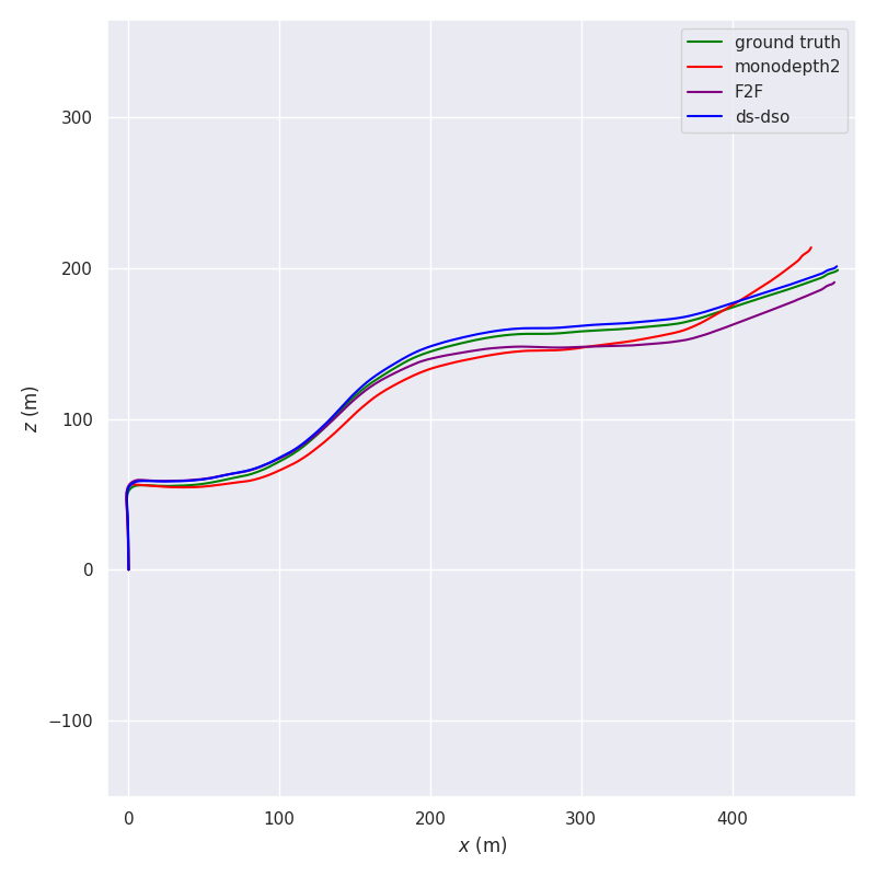
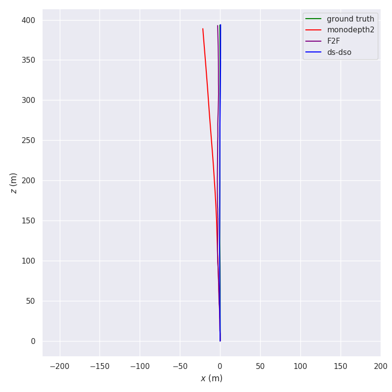
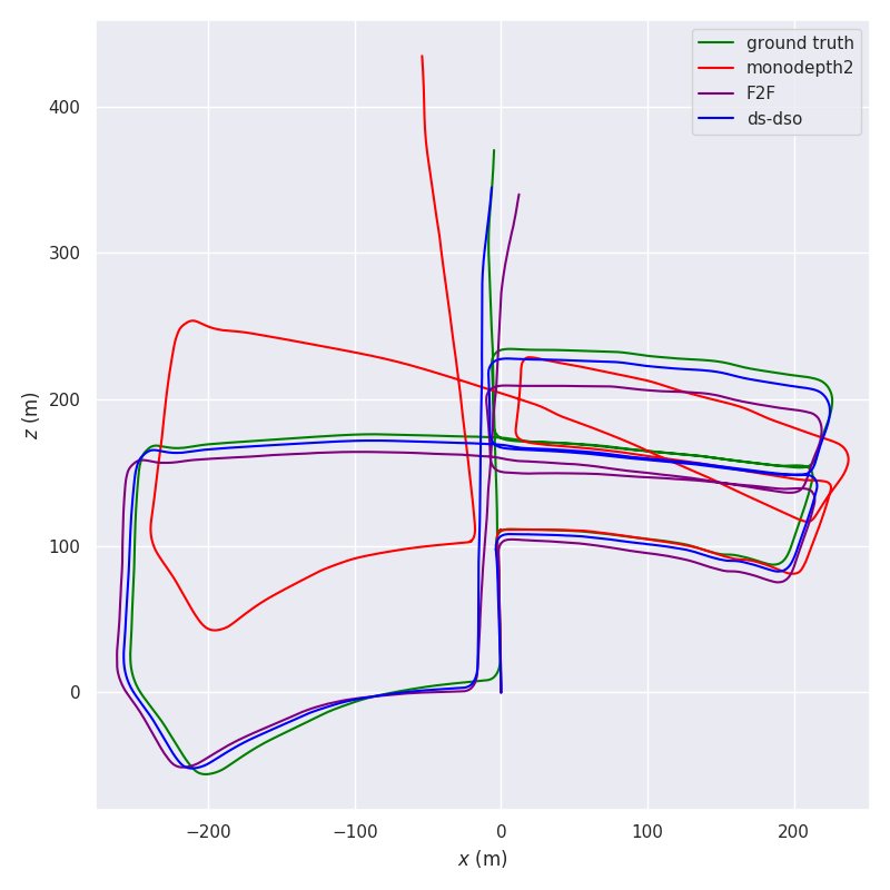
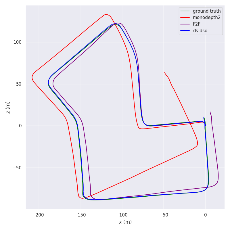
Figure 4: Qualitative trajectory estimation results on the KITTI Odometry Seq. 03, 04, 05 and 07. We compare trajectory estimation results obtained via hand-engineered keypoint matching methods against our depth-aware learned keypoint matching, with a common visual odometry backend such as DSO. As illustrated in the figure, our self-supervised method is able to accurately and robustly track stable keypoints for the task of long-term trajectory estimation.

Appendix J Keypoint Detector and Descriptor Evaluation Metrics

We follow [9] and use the Repeatability and Localization Error metrics to estimate keypoint performance and Homography Accuracy and Matching Score matrics to estimate descriptor performance. We note that for all metrics we used a distance threshold of $3$. For the Homography estimation, consistent with other reported methods, we used $300$ keypoints with the highest scores. Similarly, for the frame to frame tracking we selected $480$ keypoints to estimate the relative pose.

Repeatability is computed as the ratio of correctly associated keypoints after warping onto the target frame. We consider a warped keypoint correctly associated if the nearest keypoint in the target frame (based on Euclidean distance) is below a certain threshold.

Localization Error is computed as the average Euclidean distance between warped and associated keypoints.

Homography Accuracy To compute the homography between two images we perform reciprocal descriptor matching and we used OpenCV’s findHomography method with RANSAC, with a maximum of 5000 iterations and error threshold 3. To compute the Homography Accuracy we compare the estimated homography with the ground truth homography. Specifically we warp the image corners of the original image onto the target image using both the estimated homography and the ground truth homography, and we compute the average distance between the two sets of warped image corners, noting whether the average distance is below a certain threshold.

Matching Score is computed as the ratio between successful keypoint associations between the two images, with the association being performed using Euclidean distance in descriptor space.

Appendix K Qualitative Results on HPatches

Figure 5 shows qualitative examples of our keypoints and matches on image pairs from the HPatches dataset [47].

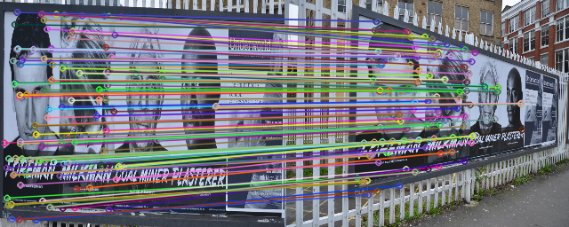
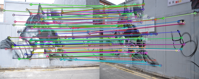
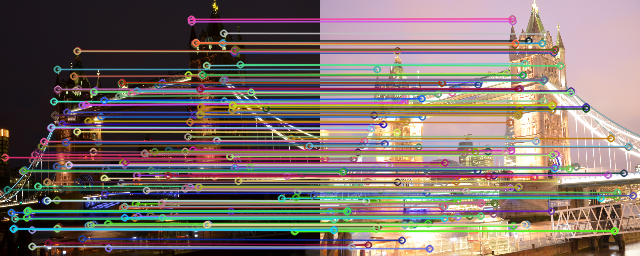
Figure 5: Qualitative matching results of our method on the HPatches dataset [47].

References

- Agarwal et al. [2010] S. Agarwal, N. Snavely, S. M. Seitz, and R. Szeliski. Bundle adjustment in the large. In European conference on computer vision, pages 29–42. Springer, 2010.
- Cadena et al. [2016] C. Cadena, L. Carlone, H. Carrillo, Y. Latif, D. Scaramuzza, J. Neira, I. Reid, and J. J. Leonard. Past, present, and future of simultaneous localization and mapping: Toward the robust-perception age. IEEE Transactions on robotics, 32(6):1309–1332, 2016.
- Lowe [1999] D. G. Lowe. Object recognition from local scale-invariant features. In Proceedings of the seventh IEEE international conference on computer vision, volume 2, pages 1150–1157. Ieee, 1999.
- Rublee et al. [2011] E. Rublee, V. Rabaud, K. Konolige, and G. Bradski. Orb: An efficient alternative to sift or surf. In 2011 International conference on computer vision, pages 2564–2571. Ieee, 2011.
- Sarlin et al. [2019] P.-E. Sarlin, C. Cadena, R. Siegwart, and M. Dymczyk. From coarse to fine: Robust hierarchical localization at large scale. In Proceedings of the IEEE Conference on Computer Vision and Pattern Recognition, pages 12716–12725, 2019.
- He et al. [2016] K. He, X. Zhang, S. Ren, and J. Sun. Deep residual learning for image recognition. In Proceedings of the IEEE conference on computer vision and pattern recognition, pages 770–778, 2016.
- Alp Güler et al. [2018] R. Alp Güler, N. Neverova, and I. Kokkinos. Densepose: Dense human pose estimation in the wild. In Proceedings of the IEEE Conference on Computer Vision and Pattern Recognition, pages 7297–7306, 2018.
- Kirillov et al. [2019] A. Kirillov, R. Girshick, K. He, and P. Dollár. Panoptic feature pyramid networks. In Proceedings of the IEEE Conference on Computer Vision and Pattern Recognition, pages 6399–6408, 2019.
- DeTone et al. [2018] D. DeTone, T. Malisiewicz, and A. Rabinovich. Superpoint: Self-supervised interest point detection and description. In Proceedings of the IEEE Conference on Computer Vision and Pattern Recognition Workshops, pages 224–236, 2018.
- Christiansen et al. [2019] P. H. Christiansen, M. F. Kragh, Y. Brodskiy, and H. Karstoft. Unsuperpoint: End-to-end unsupervised interest point detector and descriptor. arXiv preprint arXiv:1907.04011, 2019.
- Revaud et al. [2019] J. Revaud, P. Weinzaepfel, C. De Souza, N. Pion, G. Csurka, Y. Cabon, and M. Humenberger. R2d2: Repeatable and reliable detector and descriptor. arXiv preprint arXiv:1906.06195, 2019.
- Bhowmik et al. [2020] A. Bhowmik, S. Gumhold, C. Rother, and E. Brachmann. Reinforced feature points: Optimizing feature detection and description for a high-level task. In Proceedings of the IEEE/CVF Conference on Computer Vision and Pattern Recognition, pages 4948–4957, 2020.
- Engel et al. [2017] J. Engel, V. Koltun, and D. Cremers. Direct sparse odometry. IEEE transactions on pattern analysis and machine intelligence, 40(3):611–625, 2017.
- Yi et al. [2016] K. M. Yi, E. Trulls, V. Lepetit, and P. Fua. Lift: Learned invariant feature transform. In European Conference on Computer Vision, pages 467–483. Springer, 2016.
- Ono et al. [2018] Y. Ono, E. Trulls, P. Fua, and K. M. Yi. Lf-net: learning local features from images. In Advances in neural information processing systems, pages 6234–6244, 2018.
- Suwajanakorn et al. [2018] S. Suwajanakorn, N. Snavely, J. J. Tompson, and M. Norouzi. Discovery of latent 3d keypoints via end-to-end geometric reasoning. In Advances in neural information processing systems, pages 2059–2070, 2018.
- Tang et al. [2019] J. Tang, H. Kim, V. Guizilini, S. Pillai, and R. Ambrus. Neural outlier rejection for self-supervised keypoint learning. In International Conference on Learning Representations, 2019.
- Sarlin et al. [2019] P.-E. Sarlin, C. Cadena, R. Siegwart, and M. Dymczyk. From coarse to fine: Robust hierarchical localization at large scale. In The IEEE Conference on Computer Vision and Pattern Recognition (CVPR), June 2019.
- Sarlin et al. [2020] P.-E. Sarlin, D. DeTone, T. Malisiewicz, and A. Rabinovich. Superglue: Learning feature matching with graph neural networks. In Proceedings of the IEEE/CVF Conference on Computer Vision and Pattern Recognition, pages 4938–4947, 2020.
- Bai et al. [2020] X. Bai, Z. Luo, L. Zhou, H. Fu, L. Quan, and C.-L. Tai. D3feat: Joint learning of dense detection and description of 3d local features. In Proceedings of the IEEE/CVF Conference on Computer Vision and Pattern Recognition, pages 6359–6367, 2020.
- Godard et al. [2017] C. Godard, O. Mac Aodha, and G. J. Brostow. Unsupervised monocular depth estimation with left-right consistency. In Proceedings of the IEEE Conference on Computer Vision and Pattern Recognition, pages 270–279, 2017.
- Zhou et al. [2017] T. Zhou, M. Brown, N. Snavely, and D. G. Lowe. Unsupervised learning of depth and ego-motion from video. In Proceedings of the IEEE Conference on Computer Vision and Pattern Recognition, pages 1851–1858, 2017.
- Pillai et al. [2019] S. Pillai, R. Ambruş, and A. Gaidon. Superdepth: Self-supervised, super-resolved monocular depth estimation. In 2019 International Conference on Robotics and Automation (ICRA), pages 9250–9256. IEEE, 2019.
- Casser et al. [2019] V. Casser, S. Pirk, R. Mahjourian, and A. Angelova. Depth prediction without the sensors: Leveraging structure for unsupervised learning from monocular videos. In Proceedings of the AAAI Conference on Artificial Intelligence, volume 33, pages 8001–8008, 2019.
- Bian et al. [2019] J. Bian, Z. Li, N. Wang, H. Zhan, C. Shen, M.-M. Cheng, and I. Reid. Unsupervised scale-consistent depth and ego-motion learning from monocular video. In Advances in neural information processing systems, pages 35–45, 2019.
- Ambrus et al. [2019] R. Ambrus, V. Guizilini, J. Li, S. Pillai, and A. Gaidon. Two stream networks for self-supervised ego-motion estimation. In Proceedings of the 3rd International Conference on Robot Learning (CoRL), 2019.
- Luo et al. [2019] C. Luo, Z. Yang, P. Wang, Y. Wang, W. Xu, R. Nevatia, and A. Yuille. Every pixel counts++: Joint learning of geometry and motion with 3d holistic understanding. IEEE Transactions on Pattern Analysis and Machine Intelligence, 2019.
- Zhan et al. [2020] H. Zhan, C. S. Weerasekera, J.-W. Bian, and I. Reid. Visual odometry revisited: What should be learnt? In 2020 IEEE International Conference on Robotics and Automation (ICRA), pages 4203–4210. IEEE, 2020.
- Zhao et al. [2020] W. Zhao, S. Liu, Y. Shu, and Y.-J. Liu. Towards better generalization: Joint depth-pose learning without posenet. In Proceedings of the IEEE/CVF Conference on Computer Vision and Pattern Recognition, pages 9151–9161, 2020.
- Gordon et al. [2019] A. Gordon, H. Li, R. Jonschkowski, and A. Angelova. Depth from videos in the wild: Unsupervised monocular depth learning from unknown cameras. In Proceedings of the IEEE International Conference on Computer Vision, pages 8977–8986, 2019.
- Feng and Gu [2019] T. Feng and D. Gu. Sganvo: Unsupervised deep visual odometry and depth estimation with stacked generative adversarial networks. IEEE Robotics and Automation Letters, 4(4):4431–4437, 2019.
- Yang et al. [2018] N. Yang, R. Wang, J. Stuckler, and D. Cremers. Deep virtual stereo odometry: Leveraging deep depth prediction for monocular direct sparse odometry. In Proceedings of the European Conference on Computer Vision (ECCV), pages 817–833, 2018.
- Yang et al. [2020] N. Yang, L. v. Stumberg, R. Wang, and D. Cremers. D3vo: Deep depth, deep pose and deep uncertainty for monocular visual odometry. In Proceedings of the IEEE/CVF Conference on Computer Vision and Pattern Recognition, pages 1281–1292, 2020.
- Wang and Solomon [2019] Y. Wang and J. M. Solomon. Deep closest point: Learning representations for point cloud registration. In Proceedings of the IEEE International Conference on Computer Vision, pages 3523–3532, 2019.
- Choy et al. [2020] C. Choy, W. Dong, and V. Koltun. Deep global registration. In Proceedings of the IEEE/CVF Conference on Computer Vision and Pattern Recognition, pages 2514–2523, 2020.
- Krishna Murthy et al. [2020] J. Krishna Murthy, G. Iyer, and L. Paull. gradslam: Dense slam meets automatic differentiation. ICRA (to appear), 2020.
- Lepetit et al. [2009] V. Lepetit, F. Moreno-Noguer, and P. Fua. Epnp: An accurate o (n) solution to the pnp problem. International journal of computer vision, 81(2):155, 2009.
- Sheffer and Wiesel [2020] R. Sheffer and A. Wiesel. Pnp-net: A hybrid perspective-n-point network. arXiv preprint arXiv:2003.04626, 2020.
- Zhang [2000] Z. Zhang. A flexible new technique for camera calibration. IEEE Transactions on pattern analysis and machine intelligence, 22(11):1330–1334, 2000.
- Godard et al. [2019] C. Godard, O. Mac Aodha, M. Firman, and G. J. Brostow. Digging into self-supervised monocular depth estimation. In Proceedings of the IEEE international conference on computer vision, pages 3828–3838, 2019.
- Guizilini et al. [2020] V. Guizilini, R. Ambrus, S. Pillai, A. Raventos, and A. Gaidon. 3d packing for self-supervised monocular depth estimation. In Proceedings of the IEEE/CVF Conference on Computer Vision and Pattern Recognition, pages 2485–2494, 2020.
- Jaderberg et al. [2015] M. Jaderberg, K. Simonyan, A. Zisserman, et al. Spatial transformer networks. In Advances in neural information processing systems, pages 2017–2025, 2015.
- Wang et al. [2004] Z. Wang, A. C. Bovik, H. R. Sheikh, and E. P. Simoncelli. Image quality assessment: from error visibility to structural similarity. IEEE transactions on image processing, 13(4):600–612, 2004.
- Geiger et al. [2013] A. Geiger, P. Lenz, C. Stiller, and R. Urtasun. Vision meets robotics: The KITTI dataset. The International Journal of Robotics Research, 32(11):1231–1237, 2013.
- Grupp [2017] M. Grupp. evo: Python package for the evaluation of odometry and slam. https://github.com/MichaelGrupp/evo, 2017.
- Eigen et al. [2014] D. Eigen, C. Puhrsch, and R. Fergus. Depth map prediction from a single image using a multi-scale deep network. In Advances in neural information processing systems, pages 2366–2374, 2014.
- Balntas et al. [2017] V. Balntas, K. Lenc, A. Vedaldi, and K. Mikolajczyk. Hpatches: A benchmark and evaluation of handcrafted and learned local descriptors. In Proceedings of the IEEE Conference on Computer Vision and Pattern Recognition, pages 5173–5182, 2017.
- Lin et al. [2014] T.-Y. Lin, M. Maire, S. Belongie, J. Hays, P. Perona, D. Ramanan, P. Dollár, and C. L. Zitnick. Microsoft coco: Common objects in context. In European conference on computer vision, pages 740–755. Springer, 2014.
- Paszke et al. [2017] A. Paszke, S. Gross, S. Chintala, G. Chanan, E. Yang, Z. DeVito, Z. Lin, A. Desmaison, L. Antiga, and A. Lerer. Automatic differentiation in pytorch. In NIPS-W, 2017.
- Kingma and Ba [2014] D. P. Kingma and J. Ba. Adam: A method for stochastic optimization. arXiv preprint arXiv:1412.6980, 2014.
- Deng et al. [2009] J. Deng, W. Dong, R. Socher, L. jia Li, K. Li, and L. Fei-fei. Imagenet: A large-scale hierarchical image database. In Proceedings of the IEEE Conference on Computer Vision and Pattern Recognition, 2009.
- Mur-Artal and Tardós [2017] R. Mur-Artal and J. D. Tardós. Orb-slam2: An open-source slam system for monocular, stereo, and rgb-d cameras. IEEE Transactions on Robotics, 33(5):1255–1262, 2017.
- Engel et al. [2014] J. Engel, T. Schöps, and D. Cremers. Lsd-slam: Large-scale direct monocular slam. In European conference on computer vision, pages 834–849. Springer, 2014.
- Li et al. [2018] R. Li, S. Wang, Z. Long, and D. Gu. Undeepvo: Monocular visual odometry through unsupervised deep learning. In 2018 IEEE international conference on robotics and automation (ICRA), pages 7286–7291. IEEE, 2018.
- Bay et al. [2006] H. Bay, T. Tuytelaars, and L. Van Gool. Surf: Speeded up robust features. In European conference on computer vision, pages 404–417. Springer, 2006.
- Leutenegger et al. [2011] S. Leutenegger, M. Chli, and R. Siegwart. Brisk: Binary robust invariant scalable keypoints. In 2011 IEEE international conference on computer vision (ICCV), pages 2548–2555. Ieee, 2011.
- Uhrig et al. [2017] J. Uhrig, N. Schneider, L. Schneider, U. Franke, T. Brox, and A. Geiger. Sparsity invariant cnns. In 2017 International Conference on 3D Vision (3DV), pages 11–20. IEEE, 2017.
- Zhan et al. [2018] H. Zhan, R. Garg, C. Saroj Weerasekera, K. Li, H. Agarwal, and I. Reid. Unsupervised learning of monocular depth estimation and visual odometry with deep feature reconstruction. In Proceedings of the IEEE Conference on Computer Vision and Pattern Recognition, pages 340–349, 2018.