Accelerating Recommendation System Training
by Leveraging Popular Choices

Abstract.

Recommender models are commonly used to suggest relevant items to a user for e-commerce and online advertisement-based applications. These models use massive embedding tables to store numerical representation of items’ and users’ categorical variables (memory intensive) and employ neural networks (compute intensive) to generate final recommendations. Training these large-scale recommendation models is evolving to require increasing data and compute resources. The highly parallel neural networks portion of these models can benefit from GPU acceleration however, large embedding tables often cannot fit in the limited-capacity GPU device memory. Hence, this paper deep dives into the semantics of training data and obtains insights about the feature access, transfer, and usage patterns of these models. We observe that, due to the popularity of certain inputs, the accesses to the embeddings are highly skewed with a few embedding entries being accessed up to $10000\times$ more. This paper leverages this asymmetrical access pattern to offer a framework, called FAE, and proposes a hot-embedding aware data layout for training recommender models. This layout utilizes the scarce GPU memory for storing the highly accessed embeddings, thus reduces the data transfers from CPU to GPU. At the same time, FAE engages the GPU to accelerate the executions of these hot embedding entries. Experiments on production-scale recommendation models with real datasets show that FAE reduces the overall training time by 2.3$\times$ and 1.52$\times$ in comparison to XDL CPU-only and XDL CPU-GPU execution while maintaining baseline accuracy.

PVLDB Reference Format:
PVLDB, 15(1): XXX-XXX, 2022.
doi:10.14778/3485450.3485462

PVLDB Artifact Availability:
The source code, data, and/or other artifacts have been made available at https://github.com/Lab-Gattaca-UBC/Accelerating-RecSys-Training.

1. Introduction

Recommendation models are an important class of machine learning algorithms that enable the industry (Netflix (Gomez-Uribe and Hunt, 2016), Facebook (Naumov et al., 2019), Amazon (Smith and Linden, 2017), etc.) to offer a targeted user experience through personalized recommendations. Deep learning based recommendation models (Naumov et al., 2019; Ishkhanov et al., 2020) are at the core of a wide variety of internet services and consume significant infrastructure capacity and compute cycles in datacenters (Naumov et al., 2020). Training such at-scale models observes a conflation of challenges arising from high compute and data storage/transfer requirements. On the compute side, hardware accelerators notably GPUs and other heterogeneous architectures (Jouppi et al., 2017; Chung et al., 2018; Chen et al., 2014; Mahajan et al., 2016; Chen et al., 2016) provide a robust mechanism to increase performance and energy efficiency. To mitigate the large memory requirement, distributing training load through model parallel training (Narayanan et al., 2019; Huang et al., 2019; Dean et al., 2012; Jeon et al., 2019) or reducing the overall memory requirement through sparsity (Han et al., 2015) and compression (Li et al., 2016; Sun et al., 2020; Wu et al., 2020; Jain et al., 2018; Hong et al., 2019, 2018; Ghasemazar et al., 2020; Young et al., 2017) can be used. However, such techniques either require a pool of hardware accelerators that cumulatively provide enough memory to store these large models or tradeoff accuracy from the reduced precision for model footprint.

1.1. Motivation

Recommender models, as shown in Figure 1A, use embedding tables that contribute heavily towards the memory capacity requirement and neural networks that exhibit compute intensity. While neural networks can benefit from GPUs, embedding tables (10s of GBs) often cannot fit within GPU memories (Naumov et al., 2020; Huang et al., 2020; Mukherjee et al., 2021). Naively using model parallelism just to store the large embedding data across multiple GPUs is sub-optimal, as the number of GPU devices per compute node are not only fixed, but also scarce and expensive.

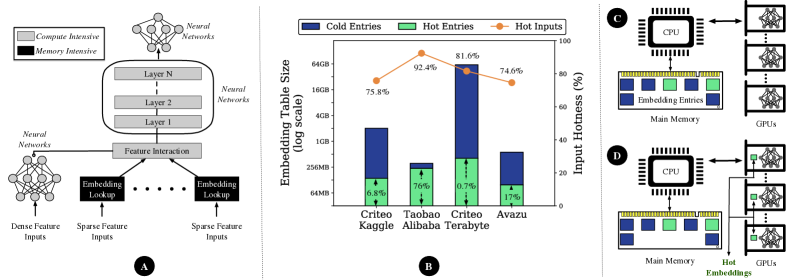
Figure 1. Typical recommender model (Naumov et al., 2019; He et al., 2017; Ishkhanov et al., 2020). They comprise compute-intensive neural networks like DNNs and MLPs in tandem with the memory-intensive embedding tables. shows embedding table sizes for four real world datasets and the proportion of the embedding table that is frequently accessed (hot). The graph also shows the % of training inputs that only access the hot embeddings. shows the baseline embedding data layout, i.e., storing entirely in the main memory. shows the proposed layout where hot embeddings that cater to ¿70% of the training inputs, are stored locally on GPUs.

Figure 1B shows the size of the embedding tables for four real-world datasets (CriteoLabs, a; Alibaba, ; CriteoLabs, b; Kaggle, ) across two open-source recommender models, “Deep Learning Recommendation Model for Personalization and Recommendation Systems” (DLRM) (Naumov et al., 2019) and “Time-based Sequence Model for Personalization and Recommendation Systems” (TBSM) (Ishkhanov et al., 2020). As user-targeted applications evolve, the size of these embedding tables is expected to increase (Rosset, 2019; Huang et al., 2020) at a rate faster than the anticipated increase in the memory capacity (Moore, 1965; Hardavellas et al., 2011). This is because larger embedding tables can track a greater and diverse degree of user preferences (Naumov et al., 2020). Therefore, in practice, it is common to train recommendation models either solely on CPUs or use the CPUs for handling the embedding data with GPUs executing data-parallel neural networks (Zhao et al., 2019). In the latter case, embeddings are stored in CPU memories as shown in Figure 1C and require embedding data to be transferred between CPU and GPUs.

Past work (Horowitz, 2014) has shown that data transfers not degrade performance but also consume significantly higher energy compared to accessing device memories. To address this, we leverage the observation that certain embedding entries and inputs to recommendation models are significantly more popular than the others. For instance, blockbuster movies tends to be significantly more popular than other movies. Below, we discuss how popular inputs and embeddings can be delegated to a faster and compute-proximate device memory while maintaining the training fidelity.

1.2. Proposed Work and Contributions

Prior work (Cho et al., 2012; Papadopoulos et al., 2012) have shown that convergence of population preferences underlies the principle of popular inputs. This popularity of training inputs implies that embedding data (accessed based on the input) also exhibits a highly skewed access behavior. Figure 1B shows the portion of the embedding entries accessed by popular inputs in real-world datasets. For each benchmark, entries that have been accessed greater than $10^{-5}$%, $10^{-6}$%, $10^{-5}$%, $10^{-5}$% of the total accesses respectively are showcased. We call these highly accessed entries and their corresponding popular inputs as hot. This paper aims to offer an embedding data layout that accounts for access patterns of such models and their training inputs. This data layout reduces the memory footprint of embedding data per GPU and mitigates frequent data transfers between CPU and GPUs.

Optimized Data Layout: The proposed optimized data layout classifies embedding entries into hot and cold regions as shown in Figure 1D. The categorization allows (1) replicating and storing only the hot embedding data (only a few hundred MBs) on every GPU device memory and (2) perform all the hot embedding accesses and neural network tensor computations locally on the GPUs. This eliminates any CPU-GPU communication for the popular inputs. For a large dataset like Criteo Terabyte, the size of hot portions of embedding tables is about $\sim$400 MB (0.7% as compared to 61GB for the entire tables) while catering to 81.6% of the input data. These hot embeddings can easily fit within the memory of even a low-end GPUs. For hot inputs, the entire graph shown in Figure 1 is trained using GPUs in a data-parallel fashion. For the remainder of the inputs, their embedding accesses and computation are performed on the CPU and the neural network is executed in data parallel fashion on GPUs.

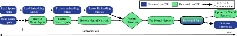
Figure 2. Execution graph of deep learning based recommender model. In this graph we show the forward graph in detail, the backward pass is a mirror of forward and executes on CPU and GPU according to its forward counterpart. The current mode of training for DLRM and TBSM requires embedding storage, reading, and processing, on CPU.

Challenges: Storing hot embedding data locally in every GPU poses four challenges: First, as each training step executes a mini-batch of inputs. If even a single input within the mini-batch accesses a cold embedding entry, that data has to be obtained from the CPU. Thus incurs a CPU-GPU communication overhead and becomes the latency bottleneck for that mini-batch. Second, training contiguously only on either hot or cold inputs can have an impact on accuracy. This is because, popular inputs only update the hot embeddings. Third, as we split hot and cold embedding data between CPU and GPUs, all the devices need to be kept synchronized. Fourth, the hotness of an embedding entry depends on the dataset and recommender model. Hence, hotness needs to be re-calibrated for every (model, dataset, and system configuration) tuple.

Contributions: This paper proposes the Frequently Accessed Embeddings (FAE) framework that efficiently places embedding data across CPUs and GPUs. while maintaining baseline accuracy. This paper makes the following contributions:

1. We find that embedding table accesses in real world recommender models is heavily skewed, thus allocating equal compute resources to all the entries is sub-optimal.

2. We intelligently place hot embeddings on every GPU device involved in training while retaining cold entries on CPUs. Placing only hot embeddings on GPUs reduces its memory requirement and improves performance. This is because FAE eliminates CPU-GPU communication for inputs that access hot embeddings and enables accelerating the compute that involves those entries.

3. To optimize training, FAE performs sampling of the input dataset to determine the access pattern of embedding tables. Thereafter, FAE classifies the input data into hot and cold categories. FAE ensures that a mini-batch either accesses only hot or only cold embeddings to avoid communication overheads. At runtime, FAE intertwines executions of hot and cold input mini-batches to ensure the baseline accuracy.

4. FAE employs statistical techniques to avoid traversing through the entire input dataset and embedding tables to determine the hot embedding access threshold and the size of the hot embedding table while incurring negligible overhead.

We prototype FAE on open-source deep learning-based recommender system training models DLRM (Naumov et al., 2019) and TBSM (Ishkhanov et al., 2020). These models are adopted by both academia (Kwon et al., 2020) and industry (Wu et al., 2019; Gupta et al., 2020; Nvidia, 2017). We compare our FAE optimized training with two implementations. First, the open-source implementations of DLRM and TBSM. Second, a highly optimized implementation of these models using the XDL framework (Jiang et al., 2019). We evaluate FAE for a wide variety of real-world and synthetic deep learning based recommender models. For real-world model architectures, our experiments show that FAE achieves an average speedup of 2.3$\times$ and 1.52$\times$ in comparison to XDL enhanced CPU and CPU-GPU baseline, respectively. Furthermore, FAE achieves 4.76$\times$ and 1.80$\times$ against DLRM and TBSM implementations on CPU and CPU-GPU, respectively. Both baselines execute in a mode that uses a CPU with 4 GPUs. FAE reduces the amount of data transferred from CPU to GPU by 1.54$\times$ in comparison to XDL-based baseline. For synthetic model architectures, FAE achieves 2.94$\times$ speedup over XDL-based baseline.

2. Background

In this section we provide the background on the model, inputs, and training process of recommendation systems.

Recommendation models and their training inputs: Figure 2 shows the flow of a recommendation model which comprises embedding lookup and neural network layers. The recommendation model has two types of inputs, namely sparse and dense. Sparse inputs typically denote specific preferences of the user (like the movie genre, choice of music, etc.) and are used by the embedding layers. Dense inputs are continuous inputs (such as time of day, location of users, etc.) that feed directly into the neural network layers. The embedding phase uses large tables containing data that reduces the sparse input feature space into a vector. These inputs are used by the Deep Neural Network (DNN) and Multi-Layer Perceptron (MLP) components to classify and determine the final recommendation.

State-of-the-art mode of execution for training. Machine learning techniques generally employ data-parallel training to reduce the overall execution time (Krizhevsky et al., 2017). This mode of training requires model replication across all the GPU devices, where each device executes on different inputs in a mini-batch. Thereafter, a post-execution synchronization is performed to update the weights/parameters using the aggregated gradient values. For recommendation models, this training mode tends to be infeasible as embedding tables cannot fit even on high-end GPUs such as Nvidia-V100.

To overcome this issue, as shown in the Figure 2, past work either executes the whole graph on the CPU or uses the CPU to handle the memory-intensive embedding layer with the GPUs executing the compute-intensive DNN layers. The first case is inefficient as CPUs are not optimized for neural network training as they cannot optimally process large tensor operations. On the other hand, the hybrid CPU-GPU mode incurs CPU-GPU communication overheads for intermediate results and gradients. This is shown in the forward pass by the bold dotted lines in the Figure 2. The backward pass also executes in a CPU-GPU mode, with CPU executing the backward computation for embeddings and GPU executing the backward propagation of neural layers. Thereafter, the gradients are generated on CPU for embeddings and on GPU for neural layers. Our experiments show that CPU-GPU communication can take up to 22% of the total training time. Additionally, any computation involving embedding data, such as the massively-parallel Stochastic Gradient Descent optimization, also then executes on the CPU.

Leveraging training input and embedding access patterns: Data accesses can exhibit locality that can be exploited either at software (Nykiel et al., 2010; Li et al., 2016), system (Kumar and Sivathanu, 2020), or hardware (Mahajan et al., 2018) level. For recommender models trained on real-world data, some sparse inputs are significantly more popular than others. Therefore, in such real-world applications, accesses into embedding tables are heavily skewed. For instance, for the Criteo Kaggle dataset (CriteoLabs, a) on DLRM, the top $6.8$% of the embedding table entries observe at least $76$% of the total accesses. It is important to note that the cold portion of the embedding data is critical from a learning perspective as it contributes to the accuracy of the model. Training only on popular inputs would make the targeted user experience futile as it would lead to certain items being always recommended. Nevertheless, from a memory perspective, as shown in Figure 1B, hot entries are more important as they form 75% to 92% of the total training input accesses.

This paper leverages the popularity semantics of training input to mitigate the bottlenecks of the above mentioned CPU-GPU execution by optimizing the embedding data layout in the memory hierarchy. Intuitively, highly accessed embeddings are kept in close proximity to the compute, i.e. GPU, whereas the cold embedding entries are stored in relatively larger but slower CPU memories. This allows us to execute the entire training graph, shown in Figure 2, on the GPU in a data-parallel fashion for the popular inputs. This data layout overcomes the limitations of the baseline by - (1) accelerating embedding compute through GPUs whilst being within the memory capacity of the device and (2) eliminating the communication overheads (gradients and activations) between CPU and GPU.

3. Challenges and Insights

To perform efficient end-to-end training with the optimized embedding layout while maintaining baseline accuracy, we require a comprehensive framework that has both static and runtime components. Next we analyze the challenges of such a training execution.

(1) Does moving the hot embedding data to the GPU suffice? As shown in Figure 3, even if 99% of the inputs are popular, i.e., access hot embeddings, the probability that the entire mini-batch accesses only hot embeddings decreases dramatically as the minibatch size increases. This is because, it is likely that at least one input within a large mini-batch would require accessing cold embedding entries. To obtain benefits from embedding data layout, we require the entire mini-batch to only access hot embedding entries. Even a single input accessing cold embedding entries would stall GPU execution as it tries to obtain its embedding entries from the CPU memory. To overcome this challenge, our framework comprises a static component that performs input-dataset pre-processing and organizes mini-batches such that they completely contain only hot or cold inputs. This pre-processing needs to be performed only once per dataset and is stored in a pre-processed format for subsequent executions. For hot mini-batches, the framework performs GPU-only data-parallel execution and for cold mini-batches the framework falls back onto the CPU-GPU hybrid mode.

Figure 3. Probability of creating a mini-batch with all popular inputs when the number of hot-inputs is 99% or lower. This reduces drastically as the mini-batch size increases.

(2) What constitutes a hot embedding entry? The classification of an embedding entry as hot or cold is based on the access threshold. Any entry that is accessed more than a threshold is classified as hot. We expose this threshold as a knob to FAE to adjust the amount of hot embeddings that can be managed by GPUs, based on both the model and system specifications. To minimize performance overhead, we devise statistical techniques that use input dataset sampling to determine the access threshold. This enables FAE to determine the optimal threshold without scanning the entire training data. FAE selects a threshold that classifies enough embedding entries as hot so that they fits in allocated GPU device memory.

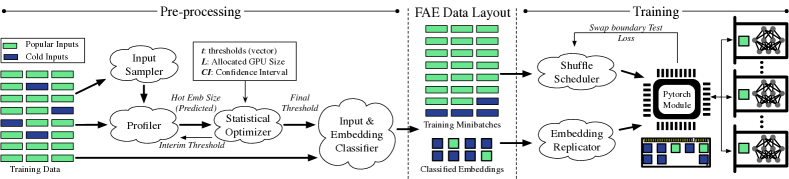
Figure 4. The FAE framework. The pre-processing phase calculates the threshold for classifying hot embeddings. This phase uses random-sampling of input datasets and embedding tables to determine the best threshold for hot embeddings. This threshold is also used to classify inputs into hot and cold mini-batches. At runtime, GPUs execute the hot input mini-batch while cold inputs execute in a CPU-GPU hybrid mode. The Shuffle Scheduler uses feedback from the pytorch modules to determine the rate of hot and cold mini-batches swap.

(3) How to schedule hot and cold mini-batches? FAE processed data contains mini-batches that are either entirely hot or cold. Scheduling all the hot mini-batches followed by cold mini-batches incurs the least embedding update overhead as the embeddings only have to synchronized between GPU and CPU once after the swap. However, such a technique can can have an non-negligible impact on the accuracy. This is because the hot mini-batches only update the hot embedding entries whereas the cold mini-batches cover more embedding entries (both hot and cold), albeit sparsely. To tackle this issue, our framework, offers a runtime solution that dynamically tunes the rate of issuing hot and cold mini-batches to ensure that the accuracy metrics are met.

(4) How to maintain consistency between the embedding tables that are scattered across devices? FAE replicates hot embedding tables across all the GPU devices and CPU contains all the embeddings (including hot embeddings). Thus, we need to perform two forms of synchronization during the training - one across all the GPUs after each mini-batch of data parallel execution and once between the cold and hot swap between CPU and GPU. In the former case, hot embeddings are synchronized using the AllReduce collectives over the fast NVlink GPU to GPU interconnect (nvl, ). In the latter case, the synchronization across GPU and CPU between hot and cold mini-batches is performed through PCIe transfer between the GPU-CPU devices. This communication overhead incurred by FAE is accounted for in the final execution latencies. To reduce this overhead, FAE minimizes the transitions between hot and cold mini-batches, without compromising baseline accuracy.

4. The FAE Framework

This paper proposes the Frequently Accessed Embeddings (FAE) framework to accelerate recommender system training. FAE efficiently utilizes the GPU memory and computation throughput to reduce the communication cost of obtaining embedding data. Figure 4 illustrates the flow of the framework; FAE consists of (1) the input and embedding pre-processing stage that determines the hotness of embeddings by sampling the input training data and (2) the training stage that replicates hot embeddings on all the GPUs and schedules hot/cold minibatches to ensure baseline accuracy. The pre-processing phase converges on an access threshold to classify an embedding entry as hot. This threshold is based on the allocated GPU memory size, confidence interval, and the CPU-GPU bandwidth. Thereafter, based on the final threshold, the Embedding Classifier and Input Classifier categorize both embedding entries and sparse inputs into hot and cold portions. The pre-processing phase executes statically once per training dataset, and stores the pre-processed data in the FAE format for subsequent training runs. At runtime, the Embedding Replicator, extracts hot embedding entries and creates embedding bags that are replicated across GPUs. The Shuffle Scheduler dynamically determines the execution order of hot and cold sparse input mini-batches across the CPU and GPUs at runtime. Based on accuracy goals, the Shuffle Scheduler interleaves hot and cold mini-batch queues to capture the updates to all embedding table entries. To help understand the next few sub-sections, Table 1 provides description of the notations for the design variables in FAE.

Table 1. List of Notations

Notation	Description
D	Training input dataset
t	Minimum number of access to classify an entry as hot
T	Total number of accesses into an embedding table
L	User-specified allocation of GPU memory for hot embeddings
h	Maximum number of hot embeddings that fit in L
Ez	Size of embedding table number z
x	Sampling rate for inputs (%)
$\widehat{\textbf{\emph{D}}}$	Sampled training input dataset entries
n	Number of Sample Chunks from the embedding logger
m	Number of entries in each embedding logger chunk (n)
N	Total m-sized entries in the embedding logger
k	For any t $\longrightarrow$ Total accesses into any embedding entry
Hzt	For any t $\longrightarrow$ Sample adjusted t per (z); minimum accesses to classify hot entries
Ci	For any t $\longrightarrow$ Number of entries in the m chunk with accesses more than Hzt
$\bar{\textbf{\emph{y}}}$	For any t $\longrightarrow$ Mean of C
s	For any t $\longrightarrow$ Standard deviation of C
CIβ	Confidence Interval of $\beta$%

4.1. Calibrating the Access Threshold

The first goal of the pre-processing phase is to pick an access threshold (t) for the embedding entries. We denote T as the total number of accesses into an embedding table. The accesses per entry for hot embeddings is $\geq$ t$\times$T. Any input that accesses only hot embeddings is also categorized as hot. Picking a large t would imply that only a few embedding entries would have enough accesses to be classified as hot. It would lead to only a small percentage of sparse-inputs that would execute completely in a GPU execution mode and thus reduce the overall performance benefits. Conversely, picking a small threshold will categorize embedding entries with very few accesses as hot which, would increase the embedding table size, often beyond the GPU device memory capacity. Figure 5 shows that we observe diminishing returns by reducing the threshold, as the number of hot embedding entries increases more steeply as compared to hot inputs. Thus, we need to efficiently tune t based on the system configuration parameters.

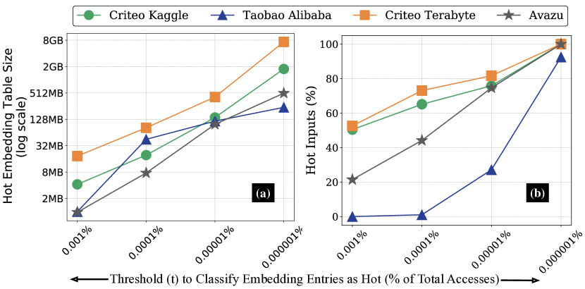
Figure 5. (a) Size of hot embedding entries and (b) Percentage of hot inputs with varying access threshold values. As we vary the threshold, the size of the embedding entries increases more rapidly compared to the percent of hot inputs

.

One of the system configuration parameters is the GPU memory allocated for hot embeddings – denoted by L. Notation h constitutes the maximum number of hot entries that fit within L. A naive mechanism to determine t will profile the entire training dataset and analyze the accesses of all the embedding entries. This requires sorting all embedding entries based on their access frequencies and classifying the top h entries as hot. This implementation will incur a high pre-processing overhead as it could imply processing several terabytes of data – even though profiling is performed only once per dataset. Instead, we propose a novel input sampler and Statistical Optimizer that ensures a low static compilation overhead for finding optimal t such that L is used effectively. Figure 6 describes the flow of events to determine the optimal value of t.

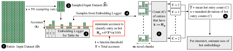
Figure 6. The flow of events in Input Sampler and Profiler. The original input is sampled at 5%. This sample is used by the profiler to create an access profile across embedding entries in the logger . For each threshold, A few chunks from the embedding logger are randomly sampled to estimate the count of hot entries . The mean and standard deviation of this count determines the size of hot embedding tables per threshold .

4.1.1. Mitigating Read Overheads with Sparse Input Sampler

As size of the training input dataset is typically very large, we sample x% of the input dataset (D). The value of x is specified as a hyper-parameter. Our implementation uses x = 5% and obtains $\widehat{\textbf{\emph{D}}}$ sampled sparse-input entries. Figure 7 shows the access profile for one large embedding table each for Criteo Kaggle, Taobao Alibaba, Criteo Terabyte, and Avazu datasets with and without input sampling. Empirically, we observe with a sampling rate of 5%, $\widehat{\textbf{\emph{D}}}$ maintains a similar access signature as D.

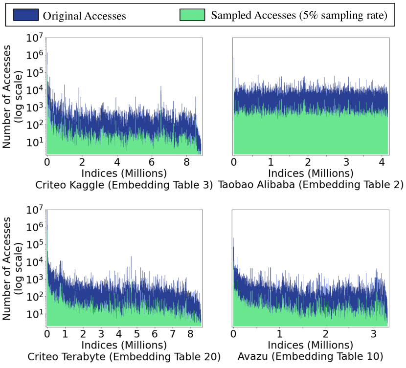
Figure 7. Embedding table access profile from the original inputs (D) and the sampled inputs ($\widehat{\textbf{\emph{D}}}$) – sampling rate (x) = 5%. We observe that $\widehat{\textbf{\emph{D}}}$ has a similar access signature to D.

As shown in Figure 8, FAE obtains 19$\times$ to 55$\times$ reduction in latency by input sampling.

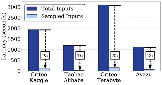
Figure 8. Reduction in the profiling latency when input dataset is sampled for embedding table access pattern.

4.1.2. Categorize and determine hot embedding size with the Profiler

The goal of the profiler is twofold - (1) for the sampled input dataset $\widehat{\textbf{\emph{D}}}$ it creates an access profile of each embedding table (E_z), where z is the table number and (2) it further samples this access profile to determine what the size of the hot embedding table is.

Embedding Logger. The profiler uses an embedding logger for each table to keep track of access counts (denoted as k) of $\widehat{\textbf{\emph{D}}}$ into each entry in E_z. As each model can access multiple embedding tables, FAE assumes any table $\geq$1 MB to be large. Embedding tables $<$ 1MB are de-facto considered “hot” as they can easily fit even on low-end GPUs. The profiler would still need to estimate the hot embedding table sizes without traversing all the embeddings.

Estimating the hot embedding table sizes per threshold. Profiler creates a sampled access profile for each embedding table entry across all the tables by selecting random chunks of embedding entries and their observed access pattern from the logger. This enables estimating the size of the hot embeddings without traversing all the tables in their entirety. As the embedding logger observes only x% of the actual inputs, we need to scale down the required access counts to classify hot data. For embedding table number z and a threshold t, the new hot embedding cutoff for each sampled entry is denoted by H_zt, described in Equation 1:

(1) $$~{}H_{zt}=t\times T\times\frac{x}{100}$$

We then pick n random samples, each consisting of m = 1024 entries entries from embedding logger for table z. Our implementation uses n = 35 and each sample consists of m = 1024 embedding entries. This chunk based sampling allows us to create a distribution of the access pattern. This paper uses Central Limit Theorem (CLT) to estimate the mean of the parent distribution. CLT has the property that, irrespective of the parent distribution, the mean of the sampled distribution will always approach the mean of the parent distribution. This is because, when the sample size n $\geq$ 30, CLT considers the sample size to be large and the sampled mean will be normal even if the sample does not originate from a Normal Distribution (Montgomery, ). As each embedding sample chunk consists m = 1024 entries, we can estimate the actual embedding table size with a precision of $\frac{1}{1024}$. For each chunk, we count (C) the number of entries with access counts (k) greater than or equal to H_zt. This is represented by Equation 2:

(2) $$~{}C_{i}=\sum_{j=1}^{m}(\text{ $k_{j}$ $\geqslant$ H${}_{zt}$})$$

For n chunks, the standard deviation is s and the mean is $\bar{\textbf{\emph{y}}}$, shown by Equation 3:

(3) $$~{}\bar{y}=\frac{\sum_{i=1}^{n}C_{i}}{n}\\$$

Figure 9 shows the latency savings from sampling embedding table instead of iterating through all the embedding access content. As the profiler scans 14x fewer embedding entries for each $t$ it reduces latency of each scan by 14.5$\times$-61$\times$.

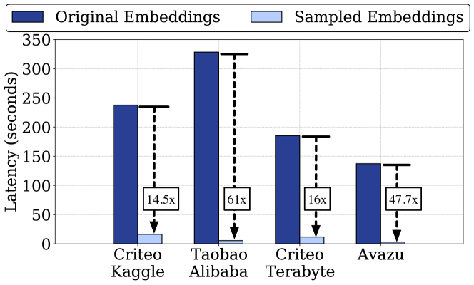
Figure 9. Reduction in the latency per iteration by using Profiler to estimate the hot embedding size per threshold. The total latency to scan all embedding tables is under 25 seconds per threshold iteration.

Input Sampler and Profiler Example: The Criteo Terabyte dataset is 45 GB in size; post Input Sampler, we only process 2.25 GB. The profiler with this sampled input dataset, logs 8.5M embeddings in the logger for embedding table 20 (E₂₀),. Assuming an interim t of $10^{-2}$ and the original training dataset of 60.5M samples, each embedding entry in the logger would have incurred at least 6.05k accesses to be categorized as hot. As we use a sampled dataset ($\widehat{\textbf{\emph{D}}}$), the hot entries observe fewer accesses and a smaller threshold of H_zt, 6.05k*$\frac{5}{100}$ = 302.5 accesses.

Confidence in the estimated embedding table size. The goal of the profiler is to establish confidence in the estimated embedding size. A confidence interval, in statistics, refers to the probability ($1-\alpha$) that a population parameter will fall between a set of values. To compute the confidence interval for the profiler’s estimated embedding table size, FAE uses the standard ‘Student’s t-interval’. As $\bar{\textbf{\emph{y}}}$ follows a t-distribution, the 100$\times$(1-$\alpha$) confidence interval (CI) for $\bar{\textbf{\emph{y}}}$ is represented by Equation 4:

(4) $$~{}CI_{100\times(1-\alpha)}=\bar{y}\pm t_{\frac{\alpha}{2}}\times\sqrt{(\frac{N-n}{N})\times(\frac{s^{2}}{n})}\\$$

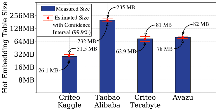
Figure 10. Estimated sizes of hot embedding tables with Profiler. For a confidence interval of 99.9%, the Profiler estimation is within 10% (upper bound) of the actual size.

Figure 10 shows the estimation variability compared to the actual values for a confidence interval of 99.9%. Actual value of the hot embedding size is the exact size the profiler would have obtained if it had processed the entire access pattern for each embedding table. This variability can be reduced if we specify a smaller confidence interval. We observe that the estimated values are within 10% of the actual values. As such, for every threshold, the profiler process described above is executed to determine the size of the hot embeddings. The Statistical Optimizer, based on this size and user requirements, either accepts the threshold or tunes it further as described below. Our experiments show that allocated memory of L = 512MB suffices for most GPUs (including low-end GPUs).

4.1.3. Converging on a Threshold using Statistical Optimizer

The Statistical Optimizer invokes the profiler with varying t (interim thresholds) and a desired confidence interval to determine the final t. Based on the embedding size estimated for an interim threshold, the optimizer tunes the threshold to be higher or lower than the previous one. This ensures that the threshold is tuned appropriately based on the available GPU memory for each model architecture. The Statistical Optimizer then provides the final threshold as output to the next blocks in the FAE.

4.2. Input and Embedding Classifier

The embedding classifier uses the output of the Embedding Logger and the final threshold from Statistical Optimizer to tag (hot or cold) the embedding table entries. This requires only one pass of each embedding table. Additionally, the input classifier uses the final access threshold value and accesses to the already classified embedding table to identify hot sparse-inputs. Typically, there are 10s of embedding tables in a recommender model. A sparse-input typically accesses one or more entries in each of these embedding tables. A sparse-input is classified as hot only if all its embedding table accesses are to hot entries. This component typically requires only one pass of the entire sparse-input ($S_{I}$) and just checks if the embedding entry indices are present in the hot-embedding bags. As this is completely parallelizable operation across both inputs and embedding indices, we divide this task across multiple cores in the CPU. For a 16 core machine (32 hardware threads), the total time for this phase for different access thresholds is given by Figure 11.

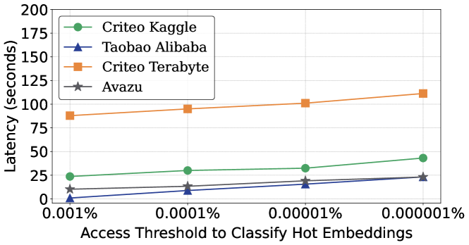
Figure 11. The latency of the input processor to classify sparse-inputs (as hot or cold) as we vary the access threshold. Overall, even for very low access thresholds, we only require only a maximum of 110 seconds.

The input classifier also bundles hot and cold inputs together into mini-batches. As aforementioned, we require the entire mini-batch to be hot to avoid the data shuffling between CPU and GPU. If an mini-batch of inputs is entirely hot, the entire execution can happen in a data-parallel mode on the GPU without any interference from the CPU. Once we have pre-processed the sparse-input data into hot and cold mini-batches, we store this in the FAE format for any subsequent training runs.

4.3. Scheduler for Dynamic Hot-Cold Swaps

FAE’s pre-processing provides a dataset that is distributed into hot and cold mini-batches and a set of hot embeddings. The Embedding Replicator replicates the hot embedding bags across all GPUs, but a note here is that the hot embeddings also are available on CPU for baseline cold input executions. Next, we discuss the runtime scheduling of hot and cold mini-batches to ensure the baseline accuracy metrics whilst providing accelerated performance.

Table 2. Model Architecture Parameters and Characteristics of the Datasets for our Workloads

Workload	Dataset	Training Input		Model Features		Embedding Tables			Neural Network Configuration
		Samples	Size	Dense	Sparse	Rows	Row Dim	Size	Bottom MLP	Top MLP	DNN
RMC1 (TBSM (Ishkhanov et al., 2020))	Taobao (Alibaba) (Alibaba, )	10 M	1 GB	3	3	5.1M	16	0.3 GB	1-16 & 22-15-15	30-60-1	Attn. Layer
RMC2 (DLRM (Naumov et al., 2019))	Criteo Kaggle (CriteoLabs, a)	45 M	2.5 GB	13	26	33.8M	16	2 GB	13-512-256-64-16	512-256-1	-
RMC3 (DLRM (Naumov et al., 2019))	Criteo Terabyte (CriteoLabs, b)	80 M	45 GB	13	26	266M	64	63 GB	13-512-256-64	512-512-256-1	-
RMC4 (DLRM (Naumov et al., 2019))	Avazu (Kaggle, )	32.3 M	2.4 GB	1	21	9.3M	16	0.55 GB	1-512-256-64-16	512-256-1	-

Impact on accuracy. In the most basic form, FAE can schedule the entire collection of mini-batches comprising hot inputs followed by cold inputs, or vice versa, but such a schedule can have potential impact on training accuracy. This is because the hot inputs only access and update the hot embedding entries, and training using only hot inputs for a long time can potentially reduce the randomness in training. For non-convexity loss optimization problems, this makes gradient descent based algorithms susceptible to local minima (Recht and Ré, 2013; Bottou, 2012). To mitigate this, machine learning community has often deployed data shuffling. Next, we discuss how we uniquely attenuate this issue for our framework.

Communication Overheads. To re-introduce randomness in our training while also attaining accelerated performance, we intermittently schedule hot and cold mini-batches. However, changing input type (hot vs cold) can degrade performance as each of these events requires synchronization of hot embedding parameters between CPU and GPU copies. To balance this tradeoff of achieving accuracy but also obtaining performance, we implement Shuffle Scheduler, a module that dynamically determines the interleaving of hot and cold mini-batches based on the runtime training metric. The scheduler always begins with training on cold inputs as they update a wider range of embedding entries, albeit infrequently. The rate of scheduling hot and cold mini-batches can be tuned dynamically based on Equation 5. In the equation, $r(i)$ is the rate at $i^{th}$ swap. Rate of ($R(100)$) implies that 100% of the mini-batches of cold inputs will be completed before the first hot mini-batches is issued. A rate of ($R(1)$) implies hot and cold are shuffled after every mini-batch. $Test_{L}$ is the testing loss and $u$ is a count of swaps.

(5) $$~{}\small r(i+1)=\begin{cases}min(r(i)*1/2,R(1))&if\Delta Test_{L}(i)\geq Test_{L}(i-1)\\ max(r(i)*2,R(100))&if\Delta Test_{L}(i)\leq Test_{L}(i-u)\\ r(i)&otherwise\end{cases}$$

Depending on the post-swap testing loss, we change the rate based on two conditions. The testing loss used for the scheduler, based on the model requirement, can be loss functions such as mean squared loss and cross-entropy logarithmic loss. All of our models and their datasets use the logarithmic loss to establish the efficacy of training. We perform a comparison of loss score between each subsequent swap. If FAE observes an increase in the test loss, it reduces the rate by half. This implies that the remaining mini-batches of hot and cold inputs will be split into an alternate of cold and hot schedules. The rate can be reduced to a minimum of $R(1)$.

If the test loss decreases, rate remains unchanged, as this is the expected behaviour, unless the loss has been decreasing successively for $u$ schedules. This is the second case where rate is changed, i.e., increased by 2, up to a max of $R(100)$. Similar to prior work that offers automatic convergence checks to avoid over-fitting, the downward trend of test loss curve (Prechelt, 1998) consecutively for 4 strips shows a balance between redundancy, badness, and slowness; thus we choose $u$ as 4. Apart from the above two cases, the rate remains unchanged. The Shuffle Scheduler ensures that accuracy remains the priority of FAE. FAE begins training with $R(50)$ (alternate cold and hot mini-batches) for a dataset, and tunes the rate accordingly.

5. Evaluation

5.1. Experimental Setup

5.1.1. Benchmarks and Real-World Datasets

We showcase the efficacy of the FAE framework on 4 real-world datasets, using recommendation models RMC1, RMC2, RMC3, and RMC4. These represent four classes of at-scale models (Gupta et al., 2020). We prototype FAE on top of the open source implementation of DLRM (Naumov et al., 2019) and TBSM (Ishkhanov et al., 2020). There is a model-dataset correspondence, based on the sparse input configuration, with RMC1 model on Taobao Alibaba (Alibaba, ) with TBSM, and RMC2 on Criteo Kaggle (CriteoLabs, a), RMC3 on Criteo Terabyte (CriteoLabs, b), and RMC4 on Avazu (Kaggle, ) with DLRM. TBSM consists of embedding layer and time series layer (TSL); the embedding layer is implemented through DLRM. TSL resembles an attention mechanism and contains its own MLP network to compute one or more context vectors between history of items and the last item. As Taobao Alibaba is the only dataset that provides temporal user-behavior to leverage the TSL layer. Table 2 describes the details of the model architecture for RMC1, RMC2, RMC3, and RMC4 including their dense and sparse features, embedding table numbers and size, and neural network configurations. In addition to these real world datasets and their corresponding models, we also perform an evaluation on synthetic models. As FAE relies on popularity of certain inputs, we execute these synthetic models on Criteo Terabyte (largest dataset) to ensure the semantics of the training input. Table 2 highlights the diversity of the model architectures in terms of embedding table sizes and neural network configurations.

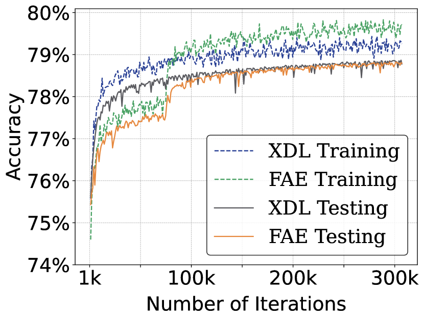
(a) Criteo Kaggle

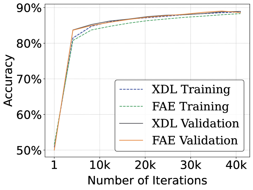
(b) Taobao Alibaba

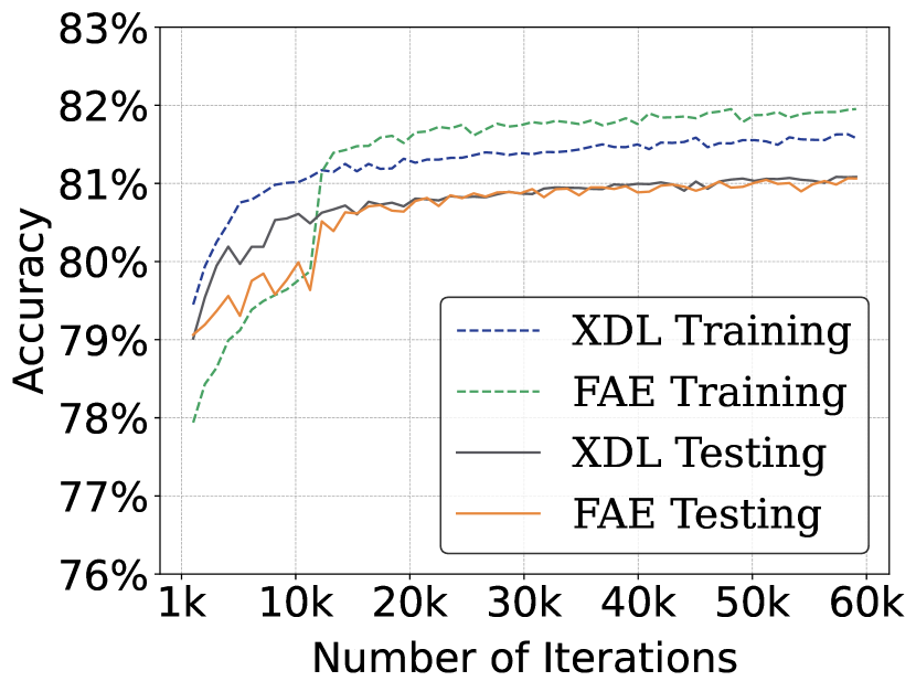
(c) Criteo Terabyte

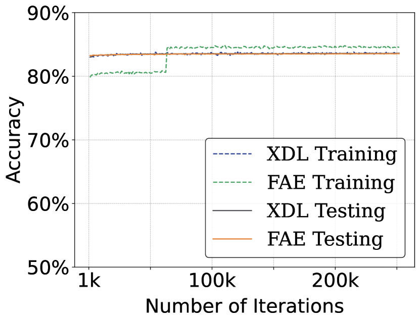
(d) Avazu

Figure 12. Increasing Accuracy with training iterations when optimized with FAE framework. As we see, all the datasets and corresponding recommender models achieve the XDL accuracy for both training and test or validation sets.

5.1.2. Software libraries and setup

The base DLRM and TBSM code is configured using the Pytorch-1.7 and executed using Python-3. We use the torch.distributed backend to support scalable distributed training and performance optimization (Paszke et al., 2017). NCCL is used (Nvidia, ) for gather, scatter, and all-reduce collective calls via the backend NVLink (nvl, ). DLRM and TBSM are also implemented on XDL 1.0 (Jiang et al., 2019) using Tensorflow-1.2 (Abadi et al., 2015) as the computation backend.

5.1.3. Server Architecture

Table 3 describes the configuration of our datacenter servers (soc, ). These servers comprise 24-core Intel Xeon Silver 4116 (2.1 GHz) processor with Skylake architecture. Each server has a DRAM memory capacity of 192 GB. Each DDR4-2666 channel has 8 GB memory. Each server also has a local storage of 1.9 TB NVMe SSD. Each server offers 4 NVIDIA Tesla-V100 each with 16GB memory capacity as a general purpose GPU. The GPUs are connected using the high speed NVLink-2.0 interconnect. Every GPU is communicating with the rest of the system via a 16x PCIe Gen3 bus. In this paper, we perform experiments on a single server with a maximum of 4 GPUs. We expect our insights to hold true even in a multi-server scenario.

Table 3. System Specifications

Device	Architecture	Memory	Storage
CPU	Intel Xeon	768 GB	1.9 TB
	Silver 4116 (2.1GHz)	DDR4 (2.7GB/s)	NVMe SSD
GPU	Nvidia Tesla	16 GB	-
	V100 (1.2GHz)	HBM-2.0 (900GB/s)

5.1.4. Baselines and terminology.

We compare FAE optimized training against two baselines: (1) An open source implementation of DLRM and TBSM and (2) A DLRM and TBSM implementation on XDL. For both baselines we execute on CPU-only mode and CPU-GPU hybrid mode with varying number of GPUs. The CPU-only mode is referred to as XDL-CPU and DLRM-CPU. For CPU-GPU hybrid mode, in case of DLRM, embeddings execute on CPU and neural networks on GPU. For XDL, GPU is used to improve the efficiency of Advance Model Server by using a faster embedding dictionary lookup on GPU. CPU is used as a backend worker. We represent this mode as X-GPU, where X is the number of GPUs. FAE optimized training is referred to as X-GPU FAE.

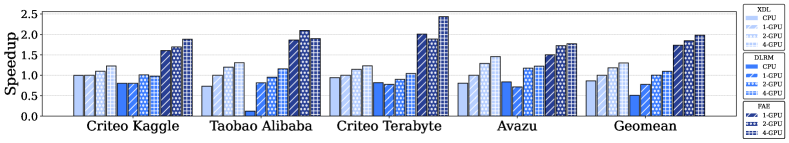
Figure 13. The performance of Criteo Kaggle, Taobao Alibaba, Criteo Terabyte, and Avazu training with the FAE vs XDL and DLRM. All values are normalized to XDL 1-GPU.

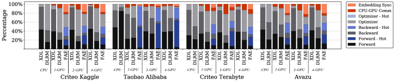
Figure 14. Latency breakdown for the 1, 2, and 4 GPU executions. The FAE framework adds the overhead of embedding synchronization across CPUs and GPUs, not present in XDL and DLRM.

5.2. Results and Insights

5.2.1. Accuracy Results

Figure 12 shows the accuracy of Criteo Kaggle, Taobao Alibaba, Criteo Terabyte, and Avazu datasets for their RMC2, RMC1, RMC3, and RMC4 models. We use a full-precision XDL-CPU execution baseline. Table 4 compares the accuracy metrics for all the workloads. We use testing accuracy, Area Under Curve (AUC), and cross-entropy loss (logloss) as recommendation model performance metric. This metric is established by the MLPerf (mlp, ) community. For Taobao dataset, we use the accuracy and logloss as performance metric, as AUC is not offered. As the table shows, each model achieves the corresponding baseline accuracy. For all the datasets, we observe that when the Shuffle Scheduler alternately issues cold and hot mini-batches at $R(50)$, the models are able to converge to the baseline accuracy in the same number of baseline training iterations. FAE observes an initial jump in accuracy for both Criteo and Avazu datasets after the first swap between cold and hot mini-batch. Once, the model is trained on both the types of mini-batches, we do not observe any more jumps. As we interleave it with the first hot mini-batch, many pertinent embedding entries get updated and we reach the baseline accuracy for both training and testing sets.

Table 4. Accuracy Metric Comparisons

Dataset	XDL			FAE
	Accuracy (%)	AUC	Logloss	Accuracy (%)	AUC	Logloss
Criteo Kaggle	78.86	0.802	0.452	78.86	0.802	0.452
Taobao Alibaba	89.21	-	0.269	89.03	-	0.271
Criteo Terabyte	81.07	0.802	0.424	81.06	0.802	0.424
Avazu	83.61	0.758	0.390	83.60	0.758	0.391

5.2.2. Performance Gains and Absolute Training Times

Figure 13 shows the performance improvement of end-to-end training execution using FAE in comparison to XDL and DLRM/TBSM. The end-to-end training runs are terminated when the established accuracy metric (cross-entropy loss or area under the curve) is met. The performance is normalized to XDL 1-GPU execution For a single device (CPU or 1-GPU), we use a mini-batch of 1K, 256, 1K and 1Kinputs for Criteo Kaggle, Taobao Alibaba, Criteo Terabyte and Avazu, respectively. FAE training reduces the average execution time (geomean) by 42%, 36%, and 34%, 1-GPU, 2-GPU, and 4-GPU executions, respectively. The GPU comparisons assume same number of GPUs for XDL and FAE. We maintain weak scaling across distributed runs where the mini-batch size is scaled with the number of GPUs. For example, 2 GPU execution use 2K, 512, 2K and 2K mini-batch size for Criteo Kaggle, Taobao Alibaba, Criteo Terabyte and Avazu, respectively. For Taobao, 4 GPU execution takes more time than 2 GPU execution because the dataset is relatively small, thus the cold mini-batch executions overshadow benefits of FAE. Overall FAE reduces the training time by 2.3$\times$ and 1.52$\times$ in comparison to XDL CPU-only and XDL CPU-GPU with 4-GPUs.

Table 5. Absolute Training Time for 10 Epochs (mins)

Dataset	XDL	1-GPU		2-GPU		4-GPU
	CPU	XDL	FAE	XDL	FAE	XDL	FAE
Criteo Kaggle	197.56	196.97	122.71	179.16	116.27	160.65	104.69
Taobao Alibaba	1108.84	813.10	436.58	677.00	387.79	621.96	428.55
Criteo Terabyte	404.25	380.88	189.73	330.06	201.61	309.51	156.45
Avazu	134.28	108.24	72.07	84.04	62.73	74.20	61.15

Absolute time: Table 5 shows the absolute end-to-end training time, when the executions reach their required accuracy metric. We use minibatch of 1k, 2k, and 4k for Crtieo Kaggle, Terabyte, and Avazu datasets. We use minibatch of 256, 512 and 1k for the Taobao Alibaba dataset. We observe that the RMC1 model with Taobao Alibaba dataset obtains most benefits from GPU acceleration as it employs a relatively large DNN. FAE can further accelerate the training of this model and reduce the training time to 428 minutes with 4-GPU FAE compared to 621 minutes with 4-GPU XDL. Our results clearly show that FAE can enable GPU acceleration without incurring large data CPU-GPU transfer overheads.

5.2.3. Latency breakdown.

Figure 14 shows the breakdown of the total runtime for each of the workloads executing on CPU-only and 1, 2, and 4 GPUs. The breakdown for cold inputs are consistent across XDL, DLRM, and FAE executions. FAE is able to mitigate some of these inefficiencies by performing both the neural network and embedding updates on GPUs for the hot input mini-batches. In case of XDL, efficiency of Advanced Model Server (AMS) is improved using GPU to speed up the massively parallel optimizer and embedding dictionary lookup. Even XDL is limited by the size of GPU memory, hence only the index of embedding dictionary is stored in GPU memory. Due to small size of hot embedding tables, FAE stores the entire table in GPU memory instead of only the indices. Figure 14 also shows the percentage of time spent by XDL, DLRM/TBSM, and FAE on embedding layer data transfer. This data transfer is completely eliminated for FAE for hot mini-batches. For DLRM/TBSM implementations, the data transfer time comprises the time spent on transferring embedding data to the GPU. For XDL, the time reported is spent on transferring embedding indices and model dense parameters to the GPU.

Embedding Synchronization: One overhead imposed by FAE is from embedding synchronization while switching between cold and hot mini-batches. The embedding tables are updated across CPU and GPU memories to ensure the training process observes the same entries. This overhead is shown by the ‘embedding sync’ entry Figure 14. The Avazu dataset observes a higher percentage of embedding synchronization overhead because of its comparatively smaller embedding size. Thus the fixed transfer cost from CPU to GPU, using PCIe, is not amortized over a large data transfer. On the contrary, the Taobao dataset observes the least percentage of synchronization overhead. This can be attributed to the high percent of forward and backward time of the RMC1 recommender model due to its deep attention layer. Thus, as the recommender models become bigger with larger embedding tables and deeper neural network layers, FAE can offer higher benefits by reducing the CPU-GPU data transfer between embedding and DNN layers, whilst observing amortized embedding synchronization overheads.

Table 6. CPU-GPU data transfer time for 10 Epochs (mins)

Dataset	1-GPU			2-GPU			4-GPU
	DLRM	XDL	FAE	DLRM	XDL	FAE	DLRM	XDL	FAE
Criteo Kaggle	22.09	5.39	4.99	23.12	5.61	4.35	18.00	3.05	4.29
Taobao Alibaba	37.93	24.97	3.24	38.27	12.89	11.11	25.04	6.24	6.04
Criteo Terabyte	76.01	13.46	13.27	92.98	18.94	12.41	48.43	17.49	15.24
Avazu	13.94	6.23	2.97	12.68	3.19	3.17	11.94	2.36	2.79

Data transfer between CPU and GPU. Table 6 shows the absolute communication time to transfer the embedding layers and Table 7 shows the amount of data transferred for XDL, DLRM/TBSM and FAE execution including the embedding synchronization for FAE. On average FAE reduces the total data transfer from 37 GB with XDL to 24 GB, even including the embedding synchronization overhead, which translates to 12% improvement in CPU-GPU data transfer time. In case of XDL, all dense parameters needs to be transferred from AMS to backend workers and vice versa per training iteration. FAE only require parameters to be transferred between CPU and GPU across the hot and cold mini-batch swap.

Table 7. Amount of Data Transferred over 10 Epochs

Dataset	DLRM (GB)	XDL (GB)	FAE (GB)
Criteo Kaggle	60.89	23.16	14.99
Taobao Alibaba	1.95	0.51	0.61
Criteo Terabyte	375.06	95.60	69.58
Avazu	40.45	30.27	10.45

5.2.4. Performance improvement with varying mini-batch size

Figure 15 shows the performance benefits of FAE training over XDL execution for a 4-GPU system. Speedup is normalized to XDL execution with mini-batch size of 1K, 256, 1K and 1K for Criteo Kaggle, Taobao Alibaba, Criteo Terabyte and Avazu datasets respectively. As the mini-batch size increases, we observe higher benefits because the overheads of FAE are amortized over a larger input set. For instance, now the Embedding Replicator replicates the model fewer times. However, with XDL, we do not see such an improvement because of extra time being spent on creating and sending larger mini-batches to the backend workers.

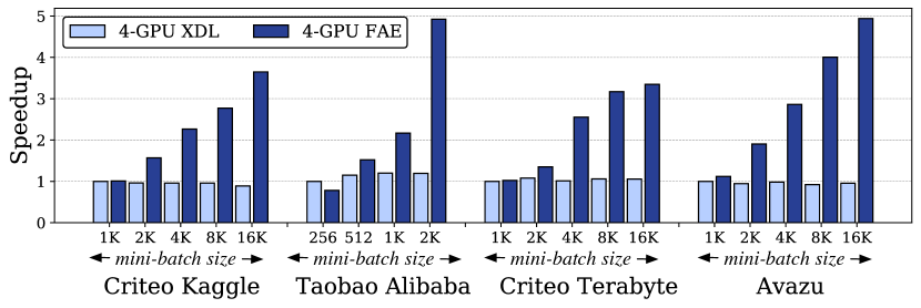
Figure 15. Speedup of FAE with varying mini-batch sizes for a 4-GPU system, compared to a 4-GPU XDL

.

5.2.5. Performance improvement for synthetic models

To understand the efficacy of FAE on varying types of model architectures, we create synthetic configurations, shown in Table 8, to execute the Terabyte dataset. Figure 16 shows the speedup of FAE across various synthetic models. FAE provides 2.94$\times$ average speedup across small and large synthetic models as compared to XDL.

Table 8. Synthetic Models’ Configuration

Dataset	Bottom MLP	Top MLP
SYN-M1	13-64	512-1
SYN-M2	13-512-64	512-256-1
SYN-M3	13-1024-512-64	512-1024-256-1
SYN-M4	13-1024-512-256-64	512-1024-512-256-1

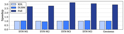
Figure 16. Performance comparison of FAE with XDL 4-GPU across various synthetic models.

5.2.6. Power Benefits

Table 9 shows the per GPU power consumption using the baseline and FAE for a 1024 mini-batch. FAE reduces GPU power consumption by 9.7% in comparison to XDL. This is primarily due to the reduced communication cost between devices.

Table 9. GPU Power Consumption Comparison

Dataset	XDL	DLRM	FAE
Criteo Kaggle	61.83W	58.91W	55.81W
Alibaba	56.39W	60.21W	56.62W
Criteo Terabyte	59.71W	62.47W	57.03W
Avazu	60.2W	58.03W	56.4W

6. Related Work

Training machine learning models is an important and heavily developed area of research. Optimizing training for deep neural networks training (Jeon et al., 2019; Chen et al., 2014; Park et al., 2017; Huang et al., 2019; Narayanan et al., 2019) has garnered most of the attention, whereas Recommender models have been under-researched.

Optimizations data layout through caching: Work in the past (Tomkins et al., 1997; Stonebraker, 1981) has delved into informed and domain-aware caching, which is highly pertinent to current applications, with their ever increasing requirement for compute and memory. In the deep learning realm, prior work (Kumar and Sivathanu, 2020) caches data on local SSD to eliminate slow reads from remote storage and employs hashing based techniques to incorporate thrashing-free strategies to efficiently utilize the shared cache. Instead, this work dives into the semantics of the training inputs observed by recommender models and offers compile time strategies to statistically ensure hot data is placed close to compute. FAE is able to fully exploit the coarse grained GPU based compute throughput without employing any dynamic hashing. Work in (Zhu et al., 2018) and (Mohan et al., 2021) employ runtime techniques to improve memory, communication, and I/O resources for training and reduce data stall time, respectively. On the hardware side, works in  (Eisenman et al., 2019) propose techniques to store embedding tables in non-volatile memories and allocate a certain portion of DRAM for caching. This work, however, does not support GPU based training executions with replicated hot embeddings and does not deal with perceptive input pre-processing to reduce communication overheads. Recent work in  (Ginart et al., 2019; Ke et al., 2020; Shi et al., 2020) has also proposed solutions to accelerate near-memory processing for embedding tables, but do not facilitate distributed training of entire recommender models using GPUs.

Embedding parameter placement: Works in (Zhao et al., 2020) offers a hierarchical parameter server that builds a distributed hash table across multiple GPUs. This work stores the working parameters close to computation, i.e, GPU, at runtime, albeit treats all embedding entries equally. Instead, FAE delves into the access pattern of each dataset and uses this information to store the highly accessed embedding entries in the GPU for the entirety of the training job. Work in (Acun et al., 2020), aims to understand the implications of different embedding table placements within an heterogeneous data-centre. However, none of the techniques leverage runtime access skew for their embedding table placement that can improve the overall training performance.

Mitigating memory intensive training through compression, sparsity, and quantization: Past work has used compression (Sun et al., 2020; Jain et al., 2018; Wu et al., 2020), sparsity (Fowers et al., 2014), and quantization (Han et al., 2015) to reduce the overall memory footprint of machine learning models. Prior work in (Nvidia Inc. Vinh Nguyen, ), optimizes training by modifying the model either through mixed-precision training or eliminating rare categorical variables to reduce the embedding table size. Even with these optimizations real dataset’s entire embedding table cannot fit on a GPU. Moreover, approaches that change the data representation and/or embedding tables, require accuracy re-validation across a variety of models and datasets. FAE enables apropos utilization of memory hierarchy without employing overheads such as compression/decompression (Li et al., 2016) and sparse operations. FAE moreover performs full-precision training of the baseline model by leveraging the highly skewed access pattern for embedded tables and increase the throughput for hot embedding entries. Nevertheless, our framework is orthogonal to the prior techniques and can be used in tandem with them to improve the memory efficiency even further.

Distributed deep learning training: Data parallel training (Krizhevsky et al., 2017) forms the most common form of distributed training as it only requires synchronization after the gradients generated in backward pass of training. As models become bigger and bigger (Rosset, 2019; Shoeybi et al., 2019), model parallelism (Chilimbi et al., 2014; Huang et al., 2019) and pipeline parallelism (Narayanan et al., 2019) are becoming common as they split a single model onto multiple devices. Nonetheless, the techniques employed to automatically split the models (Jia et al., 2019; Tarnawski et al., 2020), offer model parallelism solutions to enable training of large model with size constrained by the accelerator memory capacity. However, none of these techniques dive into the semantics of input data to perform an optimal split. This is because they are mainly suitable for DNNs.

7. Conclusions

Recommendation models aim to learn user preferences and provide a targeted user experience by employing very large embedding tables. Even though these tables often cannot fit on GPU memory, these models also comprise neural network layers that are well suited for GPUs. These contrasting requirements splits the training execution on CPUs (for memory capacity) and GPUs (for compute throughput). Fortunately, for real-world data, we observe that embedding tables exhibit a skewed data access pattern. This can be attributed to certain training inputs (users and items) that are much more popular than the others. This observation allows us to develop a comprehensive framework, namely FAE, that uses statistical techniques to quantify the hotness of embedding entries based on the input dataset. This hotness of embedding tables in turn allows the framework to optimally layout embedding so that the GPU memory is efficiently utilized to store highly accessed data close to the compute. To capture most of the performance benefits, FAE bundles hot inputs and cold inputs in separate mini-batches. This helps FAE accelerate the hot mini-batch by executing the whole model on GPU and eliminate any CPU-GPU embedding data transfers. The training for these hot inputs happens entirely on GPUs, thus reducing any CPU-GPU communication overhead between CPU-GPU and GPU-GPU from embedding and neural network layers. Our experiments on DLRM and TBSM recommender models with real datasets show that FAE reduces the overall training time by 2.3$\times$ and 1.52$\times$ in comparison to XDL CPU-only and XDL CPU-GPU execution while maintaining baseline accuracy.

References

- Gomez-Uribe and Hunt [2016] Carlos A. Gomez-Uribe and Neil Hunt. The netflix recommender system: Algorithms, business value, and innovation. ACM Trans. Manage. Inf. Syst., 6(4), December 2016. ISSN 2158-656X. doi: 10.1145/2843948. URL https://doi.org/10.1145/2843948.
- Naumov et al. [2019] Maxim Naumov, Dheevatsa Mudigere, Hao-Jun Michael Shi, Jianyu Huang, Narayanan Sundaraman, Jongsoo Park, Xiaodong Wang, Udit Gupta, Carole-Jean Wu, Alisson G. Azzolini, Dmytro Dzhulgakov, Andrey Mallevich, Ilia Cherniavskii, Yinghai Lu, Raghuraman Krishnamoorthi, Ansha Yu, Volodymyr Kondratenko, Stephanie Pereira, Xianjie Chen, Wenlin Chen, Vijay Rao, Bill Jia, Liang Xiong, and Misha Smelyanskiy. Deep learning recommendation model for personalization and recommendation systems. CoRR, abs/1906.00091, 2019. URL https://arxiv.org/abs/1906.00091.
- Smith and Linden [2017] B. Smith and G. Linden. Two decades of recommender systems at amazon.com. IEEE Internet Computing, 21(3):12–18, 2017. doi: 10.1109/MIC.2017.72.
- Ishkhanov et al. [2020] T. Ishkhanov, M. Naumov, X. Chen, Y. Zhu, Y. Zhong, A. G. Azzolini, C. Sun, F. Jiang, A. Malevich, and L. Xiong. Time-based sequence model for personalization and recommendation systems. CoRR, abs/2008.11922, 2020. URL https://arxiv.org/abs/2008.11922.
- Naumov et al. [2020] Maxim Naumov, John Kim, Dheevatsa Mudigere, Srinivas Sridharan, Xiaodong Wang, Whitney Zhao, Serhat Yilmaz, Changkyu Kim, Hector Yuen, Mustafa Ozdal, Krishnakumar Nair, Isabel Gao, Bor-Yiing Su, Jiyan Yang, and Mikhail Smelyanskiy. Deep Learning Training in Facebook Data Centers: Design of Scale-up and Scale-out Systems. arXiv e-prints, art. arXiv:2003.09518, March 2020.
- Jouppi et al. [2017] Norman P. Jouppi, Cliff Young, Nishant Patil, David Patterson, Gaurav Agrawal, Raminder Bajwa, Sarah Bates, Suresh Bhatia, Nan Boden, Al Borchers, Rick Boyle, Pierre-luc Cantin, Clifford Chao, Chris Clark, Jeremy Coriell, Mike Daley, Matt Dau, Jeffrey Dean, Ben Gelb, Tara Vazir Ghaemmaghami, Rajendra Gottipati, William Gulland, Robert Hagmann, C. Richard Ho, Doug Hogberg, John Hu, Robert Hundt, Dan Hurt, Julian Ibarz, Aaron Jaffey, Alek Jaworski, Alexander Kaplan, Harshit Khaitan, Daniel Killebrew, Andy Koch, Naveen Kumar, Steve Lacy, James Laudon, James Law, Diemthu Le, Chris Leary, Zhuyuan Liu, Kyle Lucke, Alan Lundin, Gordon MacKean, Adriana Maggiore, Maire Mahony, Kieran Miller, Rahul Nagarajan, Ravi Narayanaswami, Ray Ni, Kathy Nix, Thomas Norrie, Mark Omernick, Narayana Penukonda, Andy Phelps, Jonathan Ross, Matt Ross, Amir Salek, Emad Samadiani, Chris Severn, Gregory Sizikov, Matthew Snelham, Jed Souter, Dan Steinberg, Andy Swing, Mercedes Tan, Gregory Thorson, Bo Tian, Horia Toma, Erick Tuttle, Vijay Vasudevan, Richard Walter, Walter Wang, Eric Wilcox, and Doe Hyun Yoon. In-datacenter performance analysis of a tensor processing unit. In Proceedings of the 44th Annual International Symposium on Computer Architecture, ISCA ’17, page 1–12, New York, NY, USA, 2017. Association for Computing Machinery. ISBN 9781450348928. doi: 10.1145/3079856.3080246. URL https://doi.org/10.1145/3079856.3080246.
- Chung et al. [2018] Eric Chung, Jeremy Fowers, Kalin Ovtcharov, , Adrian Caulfield, Todd Massengill, Ming Liu, Mahdi Ghandi, Daniel Lo, Steve Reinhardt, Shlomi Alkalay, Hari Angepat, Derek Chiou, Alessandro Forin, Doug Burger, Lisa Woods, Gabriel Weisz, Michael Haselman, and Dan Zhang. Serving dnns in real time at datacenter scale with project brainwave. IEEE Micro, 38:8–20, March 2018. URL https://www.microsoft.com/en-us/research/publication/serving-dnns-real-time-datacenter-scale-project-brainwave/.
- Chen et al. [2014] Yunji Chen, Tao Luo, Shaoli Liu, Shijin Zhang, Liqiang He, Jia Wang, Ling Li, Tianshi Chen, Zhiwei Xu, Ninghui Sun, et al. Dadiannao: A machine-learning supercomputer. In MICRO, 2014.
- Mahajan et al. [2016] Divya Mahajan, Jongse Park, Emmanuel Amaro, Hardik Sharma, Amir Yazdanbakhsh, Joon Kim, and Hadi Esmaeilzadeh. Tabla: A unified template-based framework for accelerating statistical machine learning. March 2016.
- Chen et al. [2016] Yu-Hsin Chen, Joel Emer, and Vivienne Sze. Eyeriss: A Spatial Architecture for Energy-Efficient Dataflow for Convolutional Neural Networks. In ISCA, 2016.
- Narayanan et al. [2019] Deepak Narayanan, Aaron Harlap, Amar Phanishayee, Vivek Seshadri, Nikhil R. Devanur, Gregory R. Ganger, Phillip B. Gibbons, and Matei Zaharia. Pipedream: Generalized pipeline parallelism for dnn training. In Proceedings of the 27th ACM Symposium on Operating Systems Principles, SOSP ’19, page 1–15, New York, NY, USA, 2019. Association for Computing Machinery. ISBN 9781450368735. doi: 10.1145/3341301.3359646. URL https://doi.org/10.1145/3341301.3359646.
- Huang et al. [2019] Yanping Huang, Youlong Cheng, Ankur Bapna, Orhan Firat, Dehao Chen, Mia Xu Chen, HyoukJoong Lee, Jiquan Ngiam, Quoc V. Le, Yonghui Wu, and Zhifeng Chen. Gpipe: Efficient training of giant neural networks using pipeline parallelism. In Hanna M. Wallach, Hugo Larochelle, Alina Beygelzimer, Florence d’Alché-Buc, Emily B. Fox, and Roman Garnett, editors, Advances in Neural Information Processing Systems 32: Annual Conference on Neural Information Processing Systems 2019, NeurIPS 2019, 8-14 December 2019, Vancouver, BC, Canada, pages 103–112, 2019. URL http://papers.nips.cc/paper/8305-gpipe-efficient-training-of-giant-neural-networks-using-pipeline-parallelism.
- Dean et al. [2012] Jeffrey Dean, Greg Corrado, Rajat Monga, Kai Chen, Matthieu Devin, Mark Mao, Marc' aurelio Ranzato, Andrew Senior, Paul Tucker, Ke Yang, Quoc Le, and Andrew Ng. Large scale distributed deep networks. In F. Pereira, C. J. C. Burges, L. Bottou, and K. Q. Weinberger, editors, Advances in Neural Information Processing Systems, volume 25, pages 1223–1231. Curran Associates, Inc., 2012. URL https://proceedings.neurips.cc/paper/2012/file/6aca97005c68f1206823815f66102863-Paper.pdf.
- Jeon et al. [2019] Myeongjae Jeon, Shivaram Venkataraman, Amar Phanishayee, unjie Qian, Wencong Xiao, and Fan Yang. Analysis of large-scale multi-tenant gpu clusters for dnn training workloads. In Proceedings of the 2019 USENIX Conference on Usenix Annual Technical Conference, USENIX ATC ’19, page 947–960, USA, 2019. USENIX Association. ISBN 9781939133038.
- Han et al. [2015] Song Han, Huizi Mao, and William J Dally. Deep compression: Compressing deep neural networks with pruning, trained quantization and huffman coding. arXiv preprint arXiv:1510.00149, 2015.
- Li et al. [2016] Jing Li, Hung-Wei Tseng, Chunbin Lin, Yannis Papakonstantinou, and Steven Swanson. Hippogriffdb: Balancing i/o and gpu bandwidth in big data analytics. Proc. VLDB Endow., 9(14):1647–1658, October 2016. ISSN 2150-8097. doi: 10.14778/3007328.3007331. URL https://doi.org/10.14778/3007328.3007331.
- Sun et al. [2020] Yang Sun, Fajie Yuan, Min Yang, Guoao Wei, Zhou Zhao, and Duo Liu. A generic network compression framework for sequential recommender systems. In Proceedings of the 43rd International ACM SIGIR Conference on Research and Development in Information Retrieval, SIGIR ’20, page 1299–1308, New York, NY, USA, 2020. Association for Computing Machinery. ISBN 9781450380164. doi: 10.1145/3397271.3401125. URL https://doi.org/10.1145/3397271.3401125.
- Wu et al. [2020] Xiaorui Wu, Hong Xu, Honglin Zhang, Huaming Chen, and Jian Wang. Saec: similarity-aware embedding compression in recommendation systems. In Proceedings of the 11th ACM SIGOPS Asia-Pacific Workshop on Systems, pages 82–89, 2020.
- Jain et al. [2018] A. Jain, A. Phanishayee, J. Mars, L. Tang, and G. Pekhimenko. Gist: Efficient data encoding for deep neural network training. In 2018 ACM/IEEE 45th Annual International Symposium on Computer Architecture (ISCA), pages 776–789, 2018. doi: 10.1109/ISCA.2018.00070.
- Hong et al. [2019] Seokin Hong, Bulent Abali, Alper Buyuktosunoglu, Michael B. Healy, and Prashant J. Nair. Touché: Towards ideal and efficient cache compression by mitigating tag area overheads. In Proceedings of the 52nd Annual IEEE/ACM International Symposium on Microarchitecture, MICRO ’52, page 453–465, New York, NY, USA, 2019. Association for Computing Machinery. ISBN 9781450369381. doi: 10.1145/3352460.3358281. URL https://doi.org/10.1145/3352460.3358281.
- Hong et al. [2018] Seokin Hong, Prashant J. Nair, Bulent Abali, Alper Buyuktosunoglu, Kyu-Hyoun Kim, and Michael B. Healy. Attaché: Towards ideal memory compression by mitigating metadata bandwidth overheads. In Proceedings of the 51st Annual IEEE/ACM International Symposium on Microarchitecture, MICRO-51, page 326–338. IEEE Press, 2018. ISBN 9781538662403. doi: 10.1109/MICRO.2018.00034. URL https://doi.org/10.1109/MICRO.2018.00034.
- Ghasemazar et al. [2020] Amin Ghasemazar, Prashant Nair, and Mieszko Lis. Thesaurus: Efficient cache compression via dynamic clustering. In Proceedings of the Twenty-Fifth International Conference on Architectural Support for Programming Languages and Operating Systems, ASPLOS ’20, page 527–540, New York, NY, USA, 2020. Association for Computing Machinery. ISBN 9781450371025. doi: 10.1145/3373376.3378518. URL https://doi.org/10.1145/3373376.3378518.
- Young et al. [2017] Vinson Young, Prashant J. Nair, and Moinuddin K. Qureshi. Dice: Compressing dram caches for bandwidth and capacity. In Proceedings of the 44th Annual International Symposium on Computer Architecture, ISCA ’17, page 627–638, New York, NY, USA, 2017. Association for Computing Machinery. ISBN 9781450348928. doi: 10.1145/3079856.3080243. URL https://doi.org/10.1145/3079856.3080243.
- Huang et al. [2020] Jianyu Huang, Jongsoo Park, Ping Tak Peter Tang, Andrew Tulloch, et al. Mixed-precision embedding using a cache. arXiv preprint arXiv:2010.11305, 2020.
- Mukherjee et al. [2021] Avilash Mukherjee, Kumar Saurav, Prashant Nair, Sudip Shekhar, and Mieszko Lis. A case for emerging memories in dnn accelerators. In 2021 Design, Automation Test in Europe Conference Exhibition (DATE), pages 938–941, 2021. doi: 10.23919/DATE51398.2021.9474252.
- He et al. [2017] Xiangnan He, Lizi Liao, Hanwang Zhang, Liqiang Nie, Xia Hu, and Tat-Seng Chua. Neural collaborative filtering. In Proceedings of the 26th International Conference on World Wide Web, WWW ’17, page 173–182, Republic and Canton of Geneva, CHE, 2017. International World Wide Web Conferences Steering Committee. ISBN 9781450349130. doi: 10.1145/3038912.3052569. URL https://doi.org/10.1145/3038912.3052569.
- CriteoLabs [a] CriteoLabs. Criteo display ad challenge, a. https://www.kaggle.com/c/criteo-display-ad-challenge.
- [28] Alibaba. User behavior data from taobao for recommendation. https://tianchi.aliyun.com/dataset/dataDetail?dataId=649&userId=1.
- CriteoLabs [b] CriteoLabs. Terabyte click logs, b. https://labs.criteo.com/2013/12/download-terabyte-click-logs.
- [30] Kaggle. Avazu mobile ads ctr. https://www.kaggle.com/c/avazu-ctr-prediction.
- Rosset [2019] C Rosset. Turing-nlg: A 17-billion-parameter language model by microsoft. Microsoft Blog, 2019.
- Moore [1965] Gordon E. Moore. Cramming more components onto integrated circuits. Electronics, 38(8), April 1965.
- Hardavellas et al. [2011] N. Hardavellas, M. Ferdman, B. Falsafi, and A. Ailamaki. Toward dark silicon in servers. IEEE Micro, 31(4):6–15, July–Aug. 2011.
- Zhao et al. [2019] Weijie Zhao, Jingyuan Zhang, Deping Xie, Yulei Qian, Ronglai Jia, and Ping Li. Aibox: Ctr prediction model training on a single node. In Proceedings of the 28th ACM International Conference on Information and Knowledge Management, pages 319–328, 2019.
- Horowitz [2014] M. Horowitz. 1.1 computing’s energy problem (and what we can do about it). 2014 IEEE International Solid-State Circuits Conference Digest of Technical Papers (ISSCC), pages 10–14, 2014.
- Cho et al. [2012] K. Cho, M. Lee, K. Park, T. T. Kwon, Y. Choi, and Sangheon Pack. Wave: Popularity-based and collaborative in-network caching for content-oriented networks. In 2012 Proceedings IEEE INFOCOM Workshops, pages 316–321, 2012. doi: 10.1109/INFCOMW.2012.6193512.
- Papadopoulos et al. [2012] Fragkiskos Papadopoulos, Maksim Kitsak, M. A. Serrano, Marian Boguna, and Dmitri Krioukov. Popularity versus similarity in growing networks. Nature, 489(7417):537–40, Sep 27 2012. URL https://ezproxy.library.ubc.ca/login?url=https://www-proquest-com.ezproxy.library.ubc.ca/docview/1095114119?accountid=14656. Copyright - Copyright Nature Publishing Group Sep 27, 2012; Document feature - Illustrations; Graphs; ; Last updated - 2019-09-06; CODEN - NATUAS.
- Kwon et al. [2020] Youngeun Kwon, Yunjae Lee, and Minsoo Rhu. Tensor casting: Co-designing algorithm-architecture for personalized recommendation training. arXiv preprint arXiv:2010.13100, 2020.
- Wu et al. [2019] C. Wu, D. Brooks, K. Chen, D. Chen, S. Choudhury, M. Dukhan, K. Hazelwood, E. Isaac, Y. Jia, B. Jia, T. Leyvand, H. Lu, Y. Lu, L. Qiao, B. Reagen, J. Spisak, F. Sun, A. Tulloch, P. Vajda, X. Wang, Y. Wang, B. Wasti, Y. Wu, R. Xian, S. Yoo, and P. Zhang. Machine learning at facebook: Understanding inference at the edge. In 2019 IEEE International Symposium on High Performance Computer Architecture (HPCA), pages 331–344, Feb 2019. doi: 10.1109/HPCA.2019.00048.
- Gupta et al. [2020] U. Gupta, C. Wu, X. Wang, M. Naumov, B. Reagen, D. Brooks, B. Cottel, K. Hazelwood, M. Hempstead, B. Jia, H. S. Lee, A. Malevich, D. Mudigere, M. Smelyanskiy, L. Xiong, and X. Zhang. The architectural implications of facebook’s dnn-based personalized recommendation. In 2020 IEEE International Symposium on High Performance Computer Architecture (HPCA), pages 488–501, 2020. doi: 10.1109/HPCA47549.2020.00047.
- Nvidia [2017] Nvidia. Accelerating wide deep recommender inference on gpus, 2017. https://developer.nvidia.com/blog/accelerating-wide-deep-recommender-inference-on-gpus/.
- Jiang et al. [2019] Biye Jiang, Chao Deng, Huimin Yi, Zelin Hu, Guorui Zhou, Yang Zheng, Sui Huang, Xinyang Guo, Dongyue Wang, Yue Song, Liqin Zhao, Zhi Wang, Peng Sun, Yu Zhang, Di Zhang, Jinhui Li, Jian Xu, Xiaoqiang Zhu, and Kun Gai. Xdl: An industrial deep learning framework for high-dimensional sparse data. In Proceedings of the 1st International Workshop on Deep Learning Practice for High-Dimensional Sparse Data, DLP-KDD ’19, New York, NY, USA, 2019. Association for Computing Machinery. ISBN 9781450367837. doi: 10.1145/3326937.3341255. URL https://doi.org/10.1145/3326937.3341255.
- Krizhevsky et al. [2017] Alex Krizhevsky, Ilya Sutskever, and Geoffrey E. Hinton. Imagenet classification with deep convolutional neural networks. Commun. ACM, 60(6):84–90, May 2017. ISSN 0001-0782. doi: 10.1145/3065386. URL https://doi.org/10.1145/3065386.
- Nykiel et al. [2010] Tomasz Nykiel, Michalis Potamias, Chaitanya Mishra, George Kollios, and Nick Koudas. Mrshare: Sharing across multiple queries in mapreduce. Proc. VLDB Endow., 3(1–2):494–505, September 2010. ISSN 2150-8097. doi: 10.14778/1920841.1920906. URL https://doi.org/10.14778/1920841.1920906.
- Kumar and Sivathanu [2020] Abhishek Vijaya Kumar and Muthian Sivathanu. Quiver: An informed storage cache for deep learning. In 18th USENIX Conference on File and Storage Technologies (FAST 20), pages 283–296, Santa Clara, CA, February 2020. USENIX Association. ISBN 978-1-939133-12-0. URL https://www.usenix.org/conference/fast20/presentation/kumar.
- Mahajan et al. [2018] Divya Mahajan, Joon Kyung Kim, Jacob Sacks, Adel Ardalan, Arun Kumar, and Hadi Esmaeilzadeh. In-rdbms hardware acceleration of advanced analytics. Proc. VLDB Endow., 11(11):1317–1331, July 2018. ISSN 2150-8097. doi: 10.14778/3236187.3236188. URL https://doi.org/10.14778/3236187.3236188.
- [47] Nvlink. URL https://developer.nvidia.com/nccl.
- [48] Runger Montgomery. Applied statistics and probability for engineers.
- Recht and Ré [2013] B. Recht and C. Ré. Parallel stochastic gradient algorithms for large-scale matrix completion. Mathematical Programming Computation, 5:201–226, 2013.
- Bottou [2012] Léon Bottou. Stochastic gradient descent tricks. In Neural networks: Tricks of the trade, pages 421–436. Springer, 2012.
- Prechelt [1998] Lutz Prechelt. Early stopping-but when? In Neural Networks: Tricks of the trade, pages 55–69. Springer, 1998.
- Paszke et al. [2017] Adam Paszke, Sam Gross, Soumith Chintala, Gregory Chanan, Edward Yang, Zachary DeVito, Zeming Lin, Alban Desmaison, Luca Antiga, and Adam Lerer. Automatic differentiation in pytorch. 2017.
- [53] Nvidia. NVIDIA Collective Communications Library (NCCL). https://docs.nvidia.com/deeplearning/nccl/index.html.
- Abadi et al. [2015] Martín Abadi, Ashish Agarwal, Paul Barham, Eugene Brevdo, Zhifeng Chen, Craig Citro, Greg Corrado, Andy Davis, Jeffrey Dean, Matthieu Devin, Sanjay Ghemawat, Ian Goodfellow, Andrew Harp, Geoffrey Irving, Michael Isard, Yangqing Jia, Rafal Jozefowicz, Lukasz Kaiser, Manjunath Kudlur, Josh Levenberg, Dan Mané, Rajat Monga, Sherry Moore, Derek Murray, Chris Olah, Mike Schuster, Jonathon Shlens, Benoit Steiner, Ilya Sutskever, Kunal Talwar, Paul Tucker, Vincent Vanhoucke, Vijay Vasudevan, Fernanda Viégas, Oriol Vinyals, Pete Warden, Martin Wattenberg, Martin Wicke, Yuan Yu, and Xiaoqiang Zheng. Tensorflow: Large-scale machine learning on heterogeneous distributed systems, 2015. URL http://download.tensorflow.org/paper/whitepaper2015.pdf.
- [55] UBC Advanced Research Computing, ”UBC ARC Sockeye.” UBC Advanced Research Computing, 2019, doi: 10.14288/SOCKEYE.
- [56] Mlperf becnhmarks. https://mlcommons.org/en/training-normal-10/.
- Park et al. [2017] Jongse Park, Hardik Sharma, Divya Mahajan, Joon Kyung Kim, Preston Olds, and Hadi Esmaeilzadeh. Scale-out acceleration for machine learnng. October 2017.
- Tomkins et al. [1997] Andrew Tomkins, R. Hugo Patterson, and Garth Gibson. Informed multi-process prefetching and caching. SIGMETRICS Perform. Eval. Rev., 25(1):100–114, June 1997. ISSN 0163-5999. doi: 10.1145/258623.258680. URL https://doi.org/10.1145/258623.258680.
- Stonebraker [1981] Michael Stonebraker. Operating system support for database management. Commun. ACM, 24(7):412–418, July 1981. ISSN 0001-0782. doi: 10.1145/358699.358703. URL https://doi.org/10.1145/358699.358703.
- Zhu et al. [2018] Y. Zhu, F. Chowdhury, H. Fu, A. Moody, K. Mohror, K. Sato, and W. Yu. Entropy-aware i/o pipelining for large-scale deep learning on hpc systems. In 2018 IEEE 26th International Symposium on Modeling, Analysis, and Simulation of Computer and Telecommunication Systems (MASCOTS), pages 145–156, 2018. doi: 10.1109/MASCOTS.2018.00023.
- Mohan et al. [2021] Jayashree Mohan, Amar Phanishayee, Ashish Raniwala, and Vijay Chidambaram. Analyzing and mitigating data stalls in dnn training. In VLDB 2021, January 2021. URL https://www.microsoft.com/en-us/research/publication/analyzing-and-mitigating-data-stalls-in-dnn-training/.
- Eisenman et al. [2019] Assaf Eisenman, Maxim Naumov, Darryl Gardner, Misha Smelyanskiy, Sergey Pupyrev, Kim Hazelwood, Asaf Cidon, and Sachin Katti. Bandana: Using non-volatile memory for storing deep learning models. Proceedings of Machine Learning and Systems, 1:40–52, 2019.
- Ginart et al. [2019] A. Ginart, M. Naumov, D. Mudigere, Jiyan Yang, and J. Zou. Mixed dimension embeddings with application to memory-efficient recommendation systems. ArXiv, abs/1909.11810, 2019.
- Ke et al. [2020] L. Ke, U. Gupta, B. Y. Cho, D. Brooks, V. Chandra, U. Diril, A. Firoozshahian, K. Hazelwood, B. Jia, H. S. Lee, M. Li, B. Maher, D. Mudigere, M. Naumov, M. Schatz, M. Smelyanskiy, X. Wang, B. Reagen, C. Wu, M. Hempstead, and X. Zhang. Recnmp: Accelerating personalized recommendation with near-memory processing. In 2020 ACM/IEEE 47th Annual International Symposium on Computer Architecture (ISCA), pages 790–803, 2020. doi: 10.1109/ISCA45697.2020.00070.
- Shi et al. [2020] Hao-Jun Michael Shi, Dheevatsa Mudigere, Maxim Naumov, and Jiyan Yang. Compositional Embeddings Using Complementary Partitions for Memory-Efficient Recommendation Systems, page 165–175. Association for Computing Machinery, New York, NY, USA, 2020. ISBN 9781450379984. URL https://doi.org/10.1145/3394486.3403059.
- Zhao et al. [2020] Weijie Zhao, Deping Xie, Ronglai Jia, Yulei Qian, Ruiquan Ding, Mingming Sun, and Ping Li. Distributed hierarchical gpu parameter server for massive scale deep learning ads systems, 2020.
- Acun et al. [2020] Bilge Acun, Matthew Murphy, Xiaodong Wang, Jade Nie, Carole-Jean Wu, and Kim Hazelwood. Understanding training efficiency of deep learning recommendation models at scale, 2020.
- Fowers et al. [2014] Jeremy Fowers, Kalin Ovtcharov, Karin Strauss, Eric Chung, and Greg Stitt. A high memory bandwidth fpga accelerator for sparse matrix-vector multiplication. In International Symposium on Field-Programmable Custom Computing Machines. IEEE, May 2014. URL http://research.microsoft.com/apps/pubs/default.aspx?id=217166.
- [69] Mengdi Huang Nvidia Inc. Vinh Nguyen, Tomasz Grel. Optimizing the deep learning recommendation model on nvidia gpus. https://developer.nvidia.com/blog/optimizing-dlrm-on-nvidia-gpus.
- Shoeybi et al. [2019] M. Shoeybi, M. Patwary, R. Puri, P. LeGresley, J. Casper, and Bryan Catanzaro. Megatron-lm: Training multi-billion parameter language models using model parallelism. ArXiv, abs/1909.08053, 2019.
- Chilimbi et al. [2014] Trishul Chilimbi, Yutaka Suzue, Johnson Apacible, and Karthik Kalyanaraman. Project adam: Building an efficient and scalable deep learning training system. In 11th USENIX Symposium on Operating Systems Design and Implementation (OSDI 14), pages 571–582, Broomfield, CO, October 2014. USENIX Association. ISBN 978-1-931971-16-4. URL https://www.usenix.org/conference/osdi14/technical-sessions/presentation/chilimbi.
- Jia et al. [2019] Zhihao Jia, Matei Zaharia, and Alex Aiken. Beyond data and model parallelism for deep neural networks. SysML 2019, 2019.
- Tarnawski et al. [2020] Jakub M Tarnawski, Amar Phanishayee, Nikhil Devanur, Divya Mahajan, and Fanny Nina Paravecino. Efficient algorithms for device placement of dnn graph operators. Advances in Neural Information Processing Systems, 33, 2020.