Meta-learning One-class Classifiers with Eigenvalue Solvers for Supervised Anomaly Detection

Abstract

Neural network-based anomaly detection methods have shown to achieve high performance. However, they require a large amount of training data for each task. We propose a neural network-based meta-learning method for supervised anomaly detection. The proposed method improves the anomaly detection performance on unseen tasks, which contains a few labeled normal and anomalous instances, by meta-training with various datasets. With a meta-learning framework, quick adaptation to each task and its effective backpropagation are important since the model is trained by the adaptation for each epoch. Our model enables them by formulating adaptation as a generalized eigenvalue problem with one-class classification; its global optimum solution is obtained, and the solver is differentiable. We experimentally demonstrate that the proposed method achieves better performance than existing anomaly detection and few-shot learning methods on various datasets.

1 Introduction

Anomaly detection is a task to find anomalous instances that do not conform to expected behavior in a dataset [16]. Anomaly detection has been used in a wide variety of applications [59, 34], which include network intrusion detection [20, 85], fraud detection [3], defect detection [26, 36], and disease outbreak detection [79]. Deep learning-based anomaly methods have shown to achieve high performance due to the high representation learning capability [32, 51, 69, 82, 22, 5, 44, 71, 18, 2, 89, 65, 66, 15, 71, 68, 61]. However, these methods require a large amount of training data. Recently, few-shot learning, or meta-learning, methods attract attentions for improving performance with a few labeled data [72, 8, 62, 6, 77, 74, 7, 23, 47, 39, 24, 67, 87, 21, 28, 38, 33, 11, 63, 64, 76, 56, 81, 43]. However, existing few-shot learning methods are not designed for anomaly detection. The anomalous class is difficult to be explicitly modeled since the definition of anomaly is that instances that are different from normal instances, and there would various types of anomalies; some types of anomalies might not appear in training data.

In this paper, we propose a meta-learning method for supervised anomaly detection. The proposed model is meta-trained using various datasets, such that it can improve the expected anomaly detection performance on unseen tasks with a few labeled normal and anomalous instances. We assume that normal, or non-anomalous, instances are located inside a hypersphere in a latent space, and anomalous instances are located outside the hypersphere as one-class classification-based anomaly detection methods assume [55, 73, 65, 66]. The one-class classification framework has been successfully used for anomaly detection since it does not explicitly model the anomaly class. An anomaly score of an instance is calculated by the distance between the center of the hypersphere and the instance in the latent space.

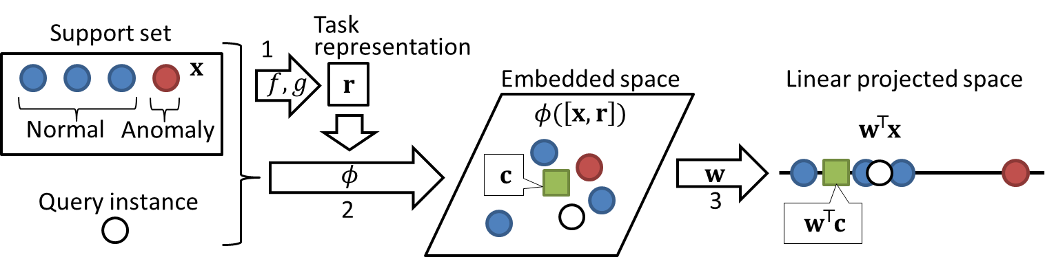
Figure 1: Our model. A blue (red) circle represents a normal (anomalous) instance in the support set, a white circle represents an unlabeled query instance, and a green square represents the center. 1) Task representation $\mathbf{r}$ is obtained using the support set by neural networks, $f$ and $g$. 2) Instances $\{\mathbf{x}\}$ in the original space are embedded into the embedded space by neural network $\phi$ using task representation $\mathbf{r}$. 3) Embedded instances $\{\phi([\mathbf{x},\mathbf{r}])\}$ and center $\mathbf{c}$ are linearly projected into a one-dimensional space by $\mathbf{w}$ such that normal support instances are located close to the center while anomalous support instances are located far away from the center. Anomaly scores are calculated by the distance from the center in the linear projected space. All neural networks, $f$, $g$, and $\phi$, and center, $\mathbf{c}$, are shared across tasks, but linear projection, $\mathbf{w}$, is task-specific and estimated using the support set.

A standard meta-learning framework learns how to adapt to small labeled data, where the gradient on the adaptation is needed for each training epoch. Therefore, it is important to quickly calculate the adaptation to each task and its gradient. We formulate the adaptation as a generalized eigenvalue problem with one-class classification-based anomaly detection. With the generalized eigenvalue problem, we can find a global optimum solution, and we can calculate the gradient of the solution in a closed form using eigenvalues and eigenvectors [1]. Existing gradient-based meta-learning methods, such as model-agnostic meta-learning [23], calculate the adaptation to each task by iterative gradient descent steps. They can only find a local optimum solution of the adaptation, and they require the gradient of the iterative gradient descent steps, which is computationally expensive.

Our model adapts to small labeled data, which is called a support set, by projecting instances into a task-specific latent space with the following procedures as illustrated in Figure 1. First, a task representation is obtained using neural networks that take the support set as input. Second, each instance is transformed into a task-specific instance representation by a neural network using the task representation. With the high representation learning power of neural networks, we can extract useful task-specific instance representations. Third, the hypersphere center and instance representations are linearly projected into a one-dimensional space by a task-specific projection to minimize the distance between the center and normal support instances while maximizing the distance between the center and anomalous support instances. The task-specific projection is obtained by solving a generalized eigenvalue problem, or in a closed form when the number of anomalous instances is one in the support set. Since the optimum solution of the projection is differentiable, we can backpropagate errors through the linear projection layer. All the neural networks in our model are shared across tasks, therefore our model is applicable to target tasks that are unseen in the training phase.

The neural networks in our model are trained by maximizing the expected test AUC using an episodic training framework [62, 70, 74, 23, 46], where support sets and test instances are randomly generated from training datasets to simulate target tasks for each epoch. The AUC is the area under the receiver operating characteristic curve. The AUC is commonly used for an evaluation measurement for anomaly detection [49].

Our major contributes are summarized as follows: 1) We propose a few-shot learning method for anomaly detection. 2) We formulate adaptation with one-class classification-based anomaly detection as a generalized eigenvalue problem, by which our model can be trained effectively to improve the expected test performance when adapted to small labeled data. 3) We experimentally demonstrate that the proposed method achieves better performance than existing anomaly detection and few-shot learning methods on various datasets.

2 Related work

Our model is based on deep support vector data description (SVDD) [65], and its supervised version [66], which achieved better anomaly detection performance than other deep learning-based methods. The SVDD embeds instances into a latent space using a neural network such that normal instances are located close to the center. Our model extends the SVDD by incorporating support set information into the embeddings, which enables us to detect anomalies with a few labeled instances for new target tasks. Although some few-shot learning methods for anomaly detection have been proposed [41, 25], these methods assume that anomaly instances are not given in target tasks, which is different from our setting.

Model-agnostic meta-learning (MAML) [23] trains the model such that the performance is improved when adapted to a support set by an iterative gradient descent method. The backpropagation through the gradient descent steps is costly in terms of memory, and thus the total number of steps must be kept small [1]. In contrast, our model adapts to a support set by solving a generalized eigenvalue problem, where a global optimum solution is obtained, and the gradient of eigenvectors is efficiently calculated using eigenvalues and eigenvectors in a closed form [1]. Ridge regression differentiable discriminator [9] and meta-learning with differentiable convex optimization [45] find a global optimum linear projection for quick adaptation in meta-learning, although they consider classification tasks, and solves a linear least square problem [9] or a convex optimization problem [45]. On the other hand, we newly design a generalized eigenvalue problem for quick adaptation in anomaly detection tasks.

Our model obtains a task representation from a support set using neural networks, which is similar to encoder-decoder style meta-learning methods [83], such as neural processes [28, 29], where adaptation is performed by neural networks. The encoder-decoder style methods can adapt quickly by forwarding the support set to neural networks. However, it is difficult to approximate the adaptation to any support data only by neural networks, and they usually require large training datasets. In contrast, the proposed method adapts a linear projection to the support data by directly solving an optimization problem.

Transfer anomaly detection methods have been proposed to transfer knowledge in source tasks to target tasks [80, 27, 4, 35, 37]. However, they require target data in a training phase. Although there are transfer anomaly detection methods that do not use target data for training [42, 17], these methods cannot use anomaly information in target data.

3 Proposed method

3.1 Problem formulation

In a training phase, we are given labeled datasets in $T$ tasks, $\{\mathcal{D}_{t}\}_{t=1}^{T}$, where $\mathcal{D}_{t}=\{(\mathbf{x}_{tn},y_{tn})\}_{n=1}^{N_{t}}$ is the $t$th task’s dataset, $\mathbf{x}_{tn}\in\mathbb{R}^{M}$ is the $n$th attribute vector, and $y_{tn}\in\{0,1\}$ is its anomaly label, $y_{tn}=1$ if it is anomaly and $y_{tn}=0$ otherwise. We assume that the attribute size $M$ is the same in all the training and target tasks. In a test phase, we are given a few labeled instances $\mathcal{S}=\{(\mathbf{x}_{n},y_{n})\}_{n=1}^{N_{\mathrm{S}}}$ in a target task, which is different from training tasks. Our aim is to identity whether unlabeled instance $\mathbf{x}$ in the target task is anomaly or not. We call a few labeled instances $\mathcal{S}$ a support set, and call unlabeled instance $\mathbf{x}$ a query.

3.2 Model

Our model outputs a task-dependent anomaly score of query $\mathbf{x}$ that is adapted to support set $\mathcal{S}$. Figure 1 illustrates our model.

First, task representation $\mathbf{r}$ is obtained with permutation invariant neural networks [88] taking support set $\mathcal{S}$ as input,

$$\mathbf{r}=g\Bigl{(}\frac{1}{N_{\mathrm{S}}}\sum_{(\mathbf{x},y)\in\mathcal{S}}f([\mathbf{x},y])\Bigr{)},$$ (1)

where $f$ and $g$ are feed-forward neural networks shared across tasks, and $[\cdot,\cdot]$ is a concatenation. Eq. (1) outputs the same value even when instances in support set $\mathcal{S}$ are permutated since the summation is permutation invariant. We use the permutation invariant neural network since the order of the instances in the support set should not affect the support set representation [28]. Then, our model obtains a representation of instance $\mathbf{x}$ that depends on the support set by nonlinearly transforming the concatenation of the instance attributes and support set representation, $\phi([\mathbf{x},\mathbf{r}])\in\mathbb{R}^{J}$, where $\phi$ is a feed-forward neural network shared across tasks.

Let $\mathbf{c}\in\mathbb{R}^{J}$ be a center where normal instances are located close to in the embedding space. The center is shared across tasks. Our model calculates an anomaly score of instance $\mathbf{x}$ by the distance between instance representation $\phi([\mathbf{x},\mathbf{r}])$ and center $\mathbf{c}$ when they are linearly projected to a one-dimensional space as follows,

$$a(\mathbf{x}|\mathcal{S})=\parallel\hat{\mathbf{w}}^{\top}\phi([\mathbf{x},\mathbf{r}])-\hat{\mathbf{w}}^{\top}\mathbf{c}\parallel^{2},$$ (2)

where $\hat{\mathbf{w}}\in\mathbb{R}^{J}$ is a task-specific linear projection vector. Instances that are located far away from $\mathbf{c}$ have high anomaly scores, and instances that are located close to $\mathbf{c}$ have low anomaly scores. We adapt $\hat{\mathbf{w}}$ to support set $\mathcal{S}$ but do not adapt the other parameters, i.e., parameters of neural networks $f$, $g$, $\phi$, and center $\mathbf{c}$. Then, the global optimum solution for adaptation is obtained in the following way without iterative gradient descent steps. We adapt projection vector $\hat{\mathbf{w}}$ to support set $\mathcal{S}$ by maximizing anomaly scores of anomalous support instances while minimizing anomaly scores of normal support instances, which is achieved by solving the following optimization problem,

$$\hat{\mathbf{w}}=\arg\max_{\mathbf{w}}\frac{\frac{1}{N_{\mathrm{A}}}\sum_{\mathbf{x}\in\mathcal{S}_{\mathrm{A}}}a(\mathbf{x}|\mathcal{S})}{\frac{1}{N_{\mathrm{N}}}\sum_{\mathbf{x}\in\mathcal{S}_{\mathrm{N}}}a(\mathbf{x}|\mathcal{S})+\eta\parallel\mathbf{w}\parallel^{2}}=\arg\max_{\mathbf{w}}\frac{\mathrm{tr}(\mathbf{w}^{\top}\mathbf{S}_{\mathrm{A}}\mathbf{w})}{\mathrm{tr}(\mathbf{w}^{\top}\mathbf{S}_{\mathrm{N}}\mathbf{w})},$$ (3)

where $\mathcal{S}_{\mathrm{A}}=\{\mathbf{x}|y=1,(\mathbf{x},y)\in\mathcal{S}\}$ is the set of anomalous support instances, $N_{\mathrm{A}}$ is its size, $\mathcal{S}_{\mathrm{N}}=\{\mathbf{x}|y=0,(\mathbf{x},y)\in\mathcal{S}\}$ is the set of normal support instances, $N_{\mathrm{N}}$ is its size, $\eta>0$ is a parameter to be trained, and

$$\mathbf{S}_{\mathrm{A}}=\frac{1}{N_{\mathrm{A}}}\sum_{\mathbf{x}\in\mathcal{S}_{\mathrm{A}}}(\phi([\mathbf{x},\mathbf{r}])-\mathbf{c})(\phi([\mathbf{x},\mathbf{r}])-\mathbf{c})^{\top},$$ (4)

$$\mathbf{S}_{\mathrm{N}}=\frac{1}{N_{\mathrm{N}}}\sum_{\mathbf{x}\in\mathcal{S}_{\mathrm{N}}}(\phi([\mathbf{x},\mathbf{r}])-\mathbf{c})(\phi([\mathbf{x},\mathbf{r}])-\mathbf{c})^{\top}+\eta\mathbf{I}.$$ (5)

The numerator of Eq. (3) is the mean of anomaly scores of anomalous support instances, and the denominator is the mean of anomaly scores of normal support instances with regularization term $\eta\parallel\mathbf{w}\parallel^{2}$. With the regularization term, $\mathbf{S}_{\mathrm{N}}$ is positive definite, and the optimization becomes stable. Note that Eq. (3) is different from the Fisher linear discriminant analysis (FLDA). FLDA maximizes the between-class covariance while minimizing the within-class covariance. In contrast, our model maximizes the distance between anomalous instances and the center while minimizing the distance between normal instances and the center.

Since Eq. (3) is a generalized Rayleigh quotient [57], we can obtain its solution by solving the following generalized eigenvalue problem in a similar way to FLDA [78, 30],

$$\mathbf{S}_{\mathrm{A}}\hat{\mathbf{w}}=\lambda\mathbf{S}_{\mathrm{N}}\hat{\mathbf{w}},$$ (6)

where $\lambda$ is the largest eigenvalue, and $\hat{\mathbf{w}}$ is its corresponding eigenvector. The eigenvector of the generalized eigenvalue problem is differentiable since it can be solved with eigenvalue decomposition and matrix inverse [78], which are differentiable. Therefore, we can backpropagate errors through the linear projection based on the generalized eigenvalue problem. The gradient of eigenvectors is efficiently calculated using eigenvalues and eigenvectors in a closed form [1]. When the dimensionality of the linearly projected space is more than one, optimization problem Eq. (3) is not a generalized Rayleigh quotient, and the solution cannot be given via a generalized eigenvalue problem [86, 19]. Therefore, instances are projected in a one-dimensional space. When the number of anomalous instances is one, there exists a simpler solution for Eq. (3),

$$\hat{\mathbf{w}}\propto\mathbf{S}_{\mathrm{N}}^{-1}(\phi([\mathbf{x}_{\mathrm{A}},\mathbf{r}])-\mathbf{c}),$$ (7)

where $\mathbf{x}_{\mathrm{A}}$ is the anomalous support instance. The derivations of Eqs. (3,7) are described in Appendices A and B.

3.3 Training

In our model, parameters to be estimated $\bm{\Theta}$ are the parameters of neural networks $f$, $g$, and $\phi$, and regularization parameter $\eta$, all of which are shared across different tasks. We determine center $\mathbf{c}$ as in SVDD [65], where after initializing the neural network parameters, we fix the center by the mean of the embeddings of the training normal instances. Note that we do not need to train task-specific linear projection vector $\hat{\mathbf{w}}$ by gradient-based methods since it is calculated by solving a generalized eigenvalue problem as shown in Section 3.2.

We train our model by maximizing the expected test AUC. Let $\mathcal{Q}$ be a query set, which is a set of query instances, and $a(\cdot|\mathcal{S})$ be the anomaly score function adapted by support set $\mathcal{S}$. The empirical AUC is given by the probability that scores of anomalous instances are higher than those of normal instances. The empirical AUC of query set $\mathcal{Q}$ with anomaly score function $a(\cdot|\mathcal{S})$ is calculated by

$$\mathrm{AUC}(\mathcal{Q}|a(\cdot|\mathcal{S}))=\frac{1}{N^{\mathrm{Q}}_{\mathrm{A}}N^{\mathrm{Q}}_{\mathrm{N}}}\sum_{\mathbf{x}\in\mathcal{Q}_{\mathrm{A}}}\sum_{\mathbf{x^{\prime}}\in\mathcal{Q}_{\mathrm{N}}}I(a(\mathbf{x}|\mathcal{S})>a(\mathbf{x}^{\prime}|\mathcal{S})),$$ (8)

where $I$ is the indicator function, $I(A)=1$ if $A$ is true, $I(A)=0$ otherwise, $\mathcal{Q}_{\mathrm{A}}$ is a set of anomalous query instances, $N_{\mathrm{A}}^{\mathrm{Q}}$ is its size, $\mathcal{Q}_{\mathrm{N}}$ is a set of normal query instances, and $N_{\mathrm{N}}^{\mathrm{Q}}$ is its size. The indicator function is not differentiable. To make the empirical AUC differentiable, we use sigmoid function $\sigma(a(\mathbf{x}|\mathcal{S})-a(\mathbf{x}^{\prime}|\mathcal{S}))=\frac{1}{1+\exp(-(a(\mathbf{x}|\mathcal{S})-a(\mathbf{x}^{\prime}|\mathcal{S})))}$ instead of indicator function $I(a(\mathbf{x}|\mathcal{S})>a(\mathbf{x}^{\prime}|\mathcal{S}))$, which is often used for a smooth approximation of the indicator function [50]. Let

$$\widetilde{\mathrm{AUC}}(\mathcal{Q}|a(\cdot|\mathcal{S}))=\frac{1}{N^{\mathrm{Q}}_{\mathrm{A}}N^{\mathrm{Q}}_{\mathrm{N}}}\sum_{\mathbf{x}\in\mathcal{Q}_{\mathrm{A}}}\sum_{\mathbf{x^{\prime}}\in\mathcal{Q}_{\mathrm{N}}}\sigma(a(\mathbf{x}|\mathcal{S})-a(\mathbf{x}^{\prime}|\mathcal{S})),$$ (9)

be a smoothed version of $\mathrm{AUC}(\mathcal{Q}|a(\cdot|\mathcal{S}))$. The objective function to be maximized is the expected smoothed test empirical AUC as follows,

$$\mathbb{E}_{t\sim\{1,\cdots,T\}}[\mathbb{E}_{(\mathcal{S},\mathcal{Q})\sim\mathcal{D}_{t}}[\widetilde{\mathrm{AUC}}(\mathcal{Q}|a(\cdot|\mathcal{S}))]],$$ (10)

where $\mathbb{E}$ represents an expectation. The objective function is maximized using an episodic training framework [62, 70, 74, 23, 46], where support and query sets are randomly generated from training datasets to simulate target tasks for each epoch. Algorithm 1 shows the training procedure for our model. In Line 2, we fix center $\mathbf{c}$ as in SVDD [65] by the mean of the embeddings of the training normal instances using the neural networks with the initial model parameters. In Lines 4–6, we generate support and query set from training datasets to simulate a target task. We obtain the projection vector using the support set in Line 7. The loss, which is the negative smoothed AUC, and its gradients are calculated in Line 8. In Line 9, we update the model parameters with a stochastic gradient-based method, such as Adam [40].

The computational complexity of each training step for each task is: $O(N_{\mathrm{S}})$ for obtaining task representation $\mathbf{r}$ using the support set in Eq. (1), $O(N_{\mathrm{S}}+N_{\mathrm{S}}+N_{\mathrm{A}}^{\mathrm{Q}}+N_{\mathrm{N}}^{\mathrm{Q}})$ for calculating instance representations $\phi([\mathbf{x},\mathbf{r}])$ for all instances in the support and query sets, $O(J^{3})$ for solving the generalized eigenvalue problem in Eq. (3), and $O(N_{\mathrm{A}}^{\mathrm{Q}}N_{\mathrm{N}}^{\mathrm{Q}})$ for evaluating the empirical AUC in Eq. (8). Although $O(J^{3})$ is a demanding part, since $J$ is the output layer size of neural network $\phi$, we can control $J$.

Algorithm 1 Training procedure of our model. $\mathrm{RandomSample}(\mathcal{D},N)$ generates a set of $N$ elements chosen uniformly at random from set $\mathcal{D}$ without replacement.

0:  Training datasets $\{\mathcal{D}_{t}\}_{t=1}^{T}$, number of support instances $N_{\mathrm{S}}$, number of query instances $N_{\mathrm{Q}}$

0:  Trained model parameters $\bm{\Theta}$

1:  Initialize model parameters $\bm{\Theta}$

2:  Fix center $\mathbf{c}$

3:  while End condition is satisfied do

4:     Randomly select task index,$t\leftarrow\mathrm{RandomSample}(\{1,\cdots,T\},1)$

5:     Randomly generate support set,$\mathcal{S}\leftarrow\mathrm{RandomSample}(\mathcal{D}_{t},N_{\mathrm{S}})$

6:     Randomly generate query set,$\mathcal{Q}\leftarrow\mathrm{RandomSample}(\mathcal{D}_{t}\setminus\mathcal{S},N_{\mathrm{Q}})$

7:     Adapt anomaly score function $a(\cdot|\mathcal{S})$ to support set $\mathcal{S}$ by solving a generalized eigenvalue problem in Eq. (6)

8:     Using the adapted anomaly score function, calculate loss $-\widetilde{\mathrm{AUC}}(\mathcal{Q}|a(\cdot|\mathcal{S}))$ and its gradients

9:     Update model parameters $\bm{\Theta}$ using the loss and its gradient

10:  end while

3.4 Only normal instances in support sets

In the previous subsections, we assume that both anomalous and normal instances are given in support sets. When only normal instances are given in support sets, we modify anomaly scores in Eq. (2) by the distance between projected instance representation $\hat{\mathbf{w}}^{\top}\phi([\mathbf{x},\mathbf{r}])$ and center $\mathbf{c}\in\mathbb{R}^{K}$ as follows, $a(\mathbf{x}|\mathcal{S})=\parallel\hat{\mathbf{W}}^{\top}\phi([\mathbf{x},\mathbf{r}])-\mathbf{c}\parallel^{2}$, where center $\mathbf{c}$ lies in the projected space, and $\hat{\mathbf{W}}\in\mathbb{R}^{J\times K}$ is the projection matrix. Projection matrix $\hat{\mathbf{W}}$ is obtained by minimizing anomaly scores of normal support instances as follows, $\hat{\mathbf{W}}=\arg\min_{\mathbf{W}}\frac{1}{N_{\mathrm{N}}}\sum_{\mathbf{x}\in\mathcal{S}_{\mathrm{N}}}a(\mathbf{x}|\mathcal{S})$. With the least squares method, its global optimum solution is given in a closed form as follows, $\hat{\mathbf{W}}=(\bm{\Phi}^{\top}\bm{\Phi})^{-1}\bm{\Phi}^{\top}\mathbf{C}$, where $\bm{\Phi}=[\phi([\mathbf{x},\mathbf{r}])]_{\mathbf{x}\in\mathcal{S}_{\mathrm{N}}}$ is an ($N_{\mathrm{N}}\times J$) matrix of instance representations, and $\mathbf{C}=[\mathbf{c},\cdots,\mathbf{c}]$ is an ($N_{\mathrm{N}}\times K$) matrix of the center.

4 Experiments

4.1 Data

We evaluated the proposed method using 22 datasets for outlier detection in [14] , Landmine dataset [84], and IoT datasets [53, 54] . Each of the 22 outlier detection datasets contained data for a single outlier detection task. We synthesized multiple tasks by multiplying a task-specific random matrix to attribute vectors, where each element of the random matrix was generated from uniform randomly with range $[-1,1]$, and the size of the random matrix was ($M\times M$), where $M$ is the number of attributes of the dataset. We generated 400 training, 50 validation, and 50 target tasks for each dataset. The Landmine dataset contained attribute vectors extracted from radar images and corresponding binary labels indicating whether landmine (anomaly) or clutter (normal) at 29 landmine fields (tasks). We randomly split the 29 tasks into 23 training, two validation, and four target tasks. The IoT datasets consisted of traffic data on nine IoT devices infected by ten types of attacks (anomaly) as well as benign (normal) traffic data. We regarded an attack type on a device as a task, where there were 80 tasks in total. We used tasks from a device for target, 90% of the other tasks for training, and the remaining tasks for validation. The statistics for each dataset are described in Appendix C. In all datasets, the number of normal support instances was $N_{\mathrm{N}}=5$, the number of anomalous support instances was $N_{\mathrm{A}}=1$, the number of normal query instances was $N^{\mathrm{Q}}_{\mathrm{N}}=25$, and the number of anomalous query instances was $N^{\mathrm{Q}}_{\mathrm{A}}=5$. We generated ten different splits of training, validation, and target tasks for each dataset, and evaluated by the test AUC on target tasks averaged over the ten splits.

4.2 Comparing methods

We compared the proposed method with the following 12 methods: SVDD, SSVDD, Proto, R2D2, MAML, FT, OSVM, IF, LOF, LR, KNN, and RF.

SVDD was deep support vector data description [65], and SSVDD was its supervised version. With SVDD, a neural network was trained so as to minimize the distance between the center and normal support instances. With SSVDD, the neural network was trained so as to maximize the AUC, where anomaly scores were calculated by the distance from the center as in the proposed method. Proto was prototypical networks [74], which was a representative few-shot learning method for classification. With Proto, attribute vectors were encoded by a neural network, and class probabilities were calculated using the negative distance from the mean of the encoded support instances for each class. R2D2 was ridge regression differentiable discriminators [9]. R2D2 was a few-shot classification method based on a neural network, where its final linear layer was determined by solving a least square problem on a support set. FT was a fine-tuning version of SSVDD, where the neural network was fine-tuned using support sets of target tasks after SSVDD was trained using training datasets. MAML was model-agnostic meta-learning [23] of SSVDD, where initial parameters of the neural network were trained so as to maximize the expected test AUC when fine-tuned using a support set. With SVDD, SSVDD, Proto, R2D2, and MAML, we used an episodic training framework. For the objective function, we used the expected test AUC with SSVDD, Proto, R2D2, FT, and MAML as in the proposed method.

OSVM was one-class support vector machines [73], IF was isolation forest [48], and LOF was local outlier factors [13], which were unsupervised anomaly detection methods. LR was logistic regression, KNN was the $k$-nearest neighbor method, and RF was random forest [12], which were supervised classification methods.

The proposed method, Proto, R2D2, MAML, and FT were meta-learning methods, where they used training datasets as well as target support sets for calculating anomaly scores of target query sets. With SVDD and SSVDD, training datasets were used for training, but target support sets were not used. OSVM, IF, LOF, LR, KNN, and RF were trained using only the support set of target tasks.

4.3 Implementation

With the proposed method, we used three-layered feed-forward neural networks for $f$ and $g$, and four-layered feed-forward neural networks for $\phi$, where their hidden and output layers contained 256 units. For neural networks with SVDD, SSVDD, Proto, R2D2, FT, MAML, we used four-layered feed-forward neural networks with 256 hidden and output units, which were the same with neural network $\phi$ with the proposed method. With SVDD and SSVDD as well as $\phi$ in the proposed method, all the bias terms from the neural networks were removed to prevent a hypersphere collapse [65]. We optimized SVDD, SSVDD, Proto, R2D2, MAML, and the proposed method using Adam [40] with learning rate $10^{-3}$, dropout rate [75] $0.1$, and batch size 256. The validation data were used for early stopping, and the maximum number of epochs was 1,000. The number of fine-tuning epochs with FT was 30, and that with MAML was five. We implemented the proposed method, SVDD, SSVDD, Proto, R2D2, MAML, and FT with PyTorch [58]. For MAML, we used Higher, which is a library for higher-order optimization [31]. We implemented OSVM, IF, LOF, LR, KNN, and RF with scikit-learn [60], and used their default parameters except for KNN, where the number of neighbors was set to one.

4.4 Results

Table 1 shows the test AUC on target tasks for each dataset. The proposed method achieved the best average performance. SVDD and SSVDD calculated anomaly scores that were independent of tasks. Therefore, their performance was low compared with the proposed method, which calculated task-dependent anomaly scores. With Proto, instances were embedded in a latent space that was the same for all tasks. Therefore, Proto could not encode characteristics for each task in the embeddings. On the other hand, the proposed method embedded instances in a task-specific latent space, which resulted in the better performance of the proposed method than Proto. Although R2D2 calculated task-specific anomaly scores, it considered anomaly detection as a standard classification problem. In contrast, the proposed method was designed for anomaly detection based on one one-class classification-based methods [55, 73, 65, 66], which have achieved good performance for anomaly detection. MAML failed to improve the performance with these datasets since it adapted the model with a small number of gradient steps. Although FT improved the performance from SSVDD by fine-tuning, the test AUC was worse than the proposed method. It is because FT trains neural networks in two separate steps: pretraining and finetuning. On the other hand, the proposed method trained neural networks such that the expected test performance was improved when optimized with small labeled data. Since OSVM, IF, LOF, LR, KNN, and RF used only target support sets for training, and could not exploit knowledge in training datasets, their test AUC was low.

Table 1: Test AUC on target tasks for each dataset. Values in bold typeface are not statistically different at 5% level from the best performing method in each dataset according to a paired t-test. The second bottom row shows the average test AUC over all datasets, and column shows the average AUC over all datasets, and the value in bold indicates the best average test AUC. The bottom row shows the number of datasets the method achieved the best or not statistically different from the best.

	Ours	SVDD	SSVDD	Proto	R2D2	MAML	FT	OSVM	IF	LOF	LR	KNN	RF
ALOI	0.999	0.920	0.983	0.999	0.995	0.290	0.650	0.781	0.781	0.833	0.947	0.531	0.876
Annthyroid	0.739	0.573	0.549	0.643	0.653	0.463	0.531	0.401	0.400	0.179	0.403	0.200	0.343
Arrhythmia	0.820	0.813	0.829	0.825	0.764	0.703	0.757	0.789	0.746	0.818	0.604	0.080	0.504
Cardiotoco.	0.988	0.537	0.484	0.526	0.884	0.504	0.277	0.953	0.849	0.965	0.919	0.177	0.492
Glass	0.952	0.682	0.657	0.879	0.894	0.649	0.719	0.836	0.802	0.253	0.881	0.473	0.674
HeartDisease	0.715	0.582	0.580	0.592	0.603	0.544	0.646	0.487	0.414	0.328	0.474	0.237	0.417
Hepatitis	0.843	0.660	0.687	0.818	0.819	0.575	0.801	0.797	0.584	0.721	0.826	0.456	0.648
InternetAds	0.788	0.759	0.795	0.739	0.693	0.721	0.740	0.802	0.740	0.617	0.732	0.000	0.491
Ionosphere	0.925	0.715	0.726	0.913	0.869	0.645	0.949	0.894	0.693	0.882	0.855	0.293	0.766
KDDCup99	0.976	0.967	0.975	0.965	0.907	0.882	0.969	0.975	0.849	0.803	0.642	0.676	0.566
Lympho.	0.943	0.887	0.937	0.932	0.769	0.687	0.929	0.882	0.668	0.798	0.705	0.356	0.625
PageBlocks	0.915	0.897	0.899	0.888	0.933	0.867	0.895	0.950	0.780	0.915	0.748	0.198	0.669
Parkinson	0.884	0.776	0.699	0.885	0.884	0.607	0.856	0.877	0.647	0.875	0.910	0.588	0.715
PenDigits	0.974	0.427	0.511	0.953	0.968	0.475	0.947	0.621	0.467	0.462	0.856	0.785	0.820
Pima	0.730	0.701	0.725	0.488	0.603	0.662	0.599	0.704	0.650	0.557	0.548	0.122	0.398
Shuttle	0.921	0.507	0.647	0.885	0.999	0.605	0.827	0.818	0.600	0.225	0.796	0.722	0.752
SpamBase	0.733	0.639	0.607	0.752	0.774	0.456	0.672	0.414	0.377	0.073	0.659	0.276	0.446
Stamps	0.946	0.871	0.897	0.828	0.930	0.797	0.935	0.966	0.865	0.933	0.847	0.477	0.762
WBC	0.997	0.998	0.997	0.990	0.947	0.988	0.993	0.992	0.991	0.913	0.108	0.188	0.836
WDBC	0.941	0.753	0.800	0.866	0.936	0.732	0.802	0.835	0.804	0.858	0.915	0.433	0.673
Waveform	0.782	0.607	0.643	0.764	0.740	0.562	0.760	0.648	0.609	0.395	0.712	0.281	0.566
Wilt	0.829	0.481	0.599	0.787	0.689	0.443	0.641	0.571	0.510	0.497	0.645	0.382	0.538
Landmine	0.922	0.749	0.898	0.603	0.821	0.876	0.829	0.834	0.693	0.650	0.745	0.217	0.574
Doorbell1	0.997	0.904	0.996	0.961	0.945	0.979	0.997	0.934	0.736	0.771	0.989	0.837	0.972
Thermostat	0.992	0.854	0.998	0.962	0.980	0.952	0.999	0.903	0.658	0.804	0.947	0.708	0.932
Doorbell2	0.990	0.795	0.995	0.972	0.954	0.949	0.991	0.868	0.688	0.461	0.934	0.504	0.740
Monitor	0.996	0.859	0.995	0.970	0.977	0.966	0.998	0.919	0.737	0.690	0.972	0.842	0.983
Camera1	0.993	0.821	0.991	0.949	0.962	0.953	0.993	0.880	0.622	0.664	0.951	0.631	0.874
Camera2	0.995	0.802	0.995	0.983	0.980	0.902	0.995	0.844	0.598	0.651	0.945	0.810	0.958
Webcam	0.998	0.833	0.999	0.987	0.990	0.945	0.999	0.923	0.674	0.826	0.971	0.804	0.983
Camera3	0.998	0.806	0.988	0.968	0.970	0.937	0.996	0.908	0.640	0.706	0.970	0.800	0.966
Camera4	0.998	0.872	0.962	0.948	0.932	0.951	0.992	0.959	0.753	0.808	0.977	0.611	0.964
Average	0.913	0.751	0.814	0.851	0.868	0.727	0.834	0.811	0.676	0.654	0.785	0.459	0.704
#Best	23	1	11	3	5	1	10	3	0	0	2	0	0

Figure 2 shows an example of visualization of support and query instances in the original, embedded and linearly projected spaces on the WDBC dataset by the proposed method. With the original space (a), an anomalous query instance (red ‘o’) was located further from the anomalous support instance (magenta ‘x’) than some normal query instances (blue ‘o’). Therefore, the anomalous query instance could not be detected as anomaly in the original space. By embedding (b), anomalous instances were located more closely together than the original space. However, there was the center (green ’$\triangle$’) near anomalous instances, and there were some normal instances in the region of anomalous instances. By linear projection (c), anomalous instances (magenta ‘x’ and red ‘o’) were located further from the center than normal instances (cyan ‘x’ and blue ‘o’), where the anomalous instances were appropriately detected by the distance from the center.

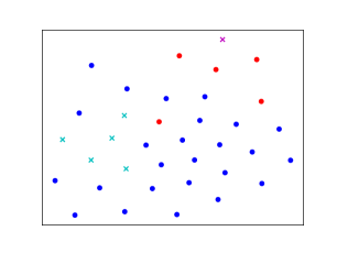
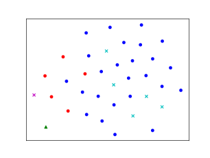
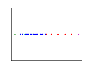
(a) Original space	(b) Embedded space	(c) Linearly projected space

Figure 2: Visualization of support and query instances in the a) original space $\mathbf{x}$, b) embedded space $\phi([\mathbf{x},\mathbf{r}])$, c) one-dimensional linearly projected space $\hat{\mathbf{w}}^{\top}\phi([\mathbf{x},\mathbf{r}])$ on the WDBC dataset by the proposed method. A cyan ‘x’ is a normal support instance, a magenta ‘x’ is an anomalous support instance, a blue ‘o’ is a normal query instance, a red ‘o’ is an anomalous query instance, and a green ‘$\triangle$’ is center. In (a) and (b), we used t-SNE [52] for visualizing in a two-dimensional space.

Table 2 shows the average test AUC on target tasks on ablation study. WoNN was the proposed method without neural networks, where original attribute vectors were linearly projected to a one-dimensional space, $\hat{\mathbf{w}}^{\top}\mathbf{x}$, where $\hat{\mathbf{w}}$ was determined by the generalized eigenvalue problem. WoProj was the proposed method without the linear projection, where anomaly scores were calculated by the distance from the center before the linear projection $a(\mathbf{x}|\mathcal{S})=\parallel\phi([\mathbf{x},\mathbf{r}])-\mathbf{c}\parallel^{2}$. WoAnomaly was the proposed method without anomalous instances, which was the method described in Section 3.4. The proposed method was better than WoNN and WoProj. This result indicates the effectiveness of the neural networks and linear projection in our model. The performance of WoAnomaly was better than existing unsupervised methods in Table 1, SVDD, OSVM, IF, and LOF. This result demonstrates the effectiveness of the proposed method without anomaly described in Section 3.4. The proposed method with anomaly improved the performance from that without anomaly by effectively using anomaly information via the neural networks with the generalized eigenvalue problem solver layer.

Table 2: Average test AUC on target tasks on ablation study of the proposed method by WoNN (without neural networks), WoProj (without linear projection), and WoAnomaly (without support anomalous instances).

Ours	WoNN	WoProj	WoAnomaly
0.913	0.880	0.874	0.853

Table 3: Average computational time in seconds for training by the proposed method, SVDD, SSVDD, Proto, R2D2, and MAML.

Ours	SVDD	SSVDD	Proto	R2D2	MAML
1,527	348	351	570	488	33,528

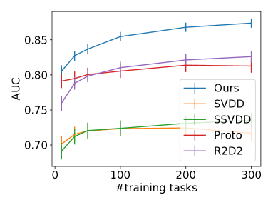
Figure 3: Average test AUC on target tasks with different numbers of training tasks on 22 outlier detection datasets.

Figure 3 shows the averaged test AUC on target tasks with different numbers of training tasks on 22 outlier detection datasets by the proposed method, SVDD, SSVDD, Proto, and R2D2. All the methods improved the performance as the number of training tasks increased. The proposed method achieved the best test AUC with all cases.

Table 3 shows the average computational time in seconds for training by the proposed method, SVDD, SSVDD, Proto, R2D2, and MAML, on computers with a 2.60GHz CPU. The proposed method had longer training time than SVDD, SVDD, Proto, and R2D2, since the proposed method calculated the task representation and linear projection for each task. However, it was much faster than MAML, which required the gradient of multiple gradient steps for each task.

5 Conclusion

We proposed a neural network-based meta-learning method for anomaly detection, where our model is trained using multiple datasets to improve the performance on unseen tasks. We experimentally confirmed the effectiveness of the proposed method compared with existing anomaly detection and few-shot learning methods. For future work, we would like to extend the proposed method for semi-supervised settings [10], where unlabeled instances, labeled normal and labeled anomalous instances are given as support sets.

Appendix A Derivation of Eq. (3)

$$\frac{1}{N_{\mathrm{A}}}\sum_{\mathbf{x}\in\mathcal{S}_{\mathrm{A}}}a(\mathbf{x}|\mathcal{S})$$

$$=\frac{1}{N_{\mathrm{A}}}\sum_{\mathbf{x}\in\mathcal{S}_{\mathrm{A}}}\parallel\hat{\mathbf{w}}^{\top}\phi([\mathbf{x},\mathbf{r}])-\hat{\mathbf{w}}^{\top}\mathbf{c}\parallel^{2}$$

$$=\frac{1}{N_{\mathrm{A}}}\sum_{\mathbf{x}\in\mathcal{S}_{\mathrm{A}}}(\hat{\mathbf{w}}^{\top}(\phi([\mathbf{x},\mathbf{r}])-\mathbf{c}))^{\top}(\hat{\mathbf{w}}^{\top}(\phi([\mathbf{x},\mathbf{r}])-\mathbf{c}))$$

$$=\frac{1}{N_{\mathrm{A}}}\sum_{\mathbf{x}\in\mathcal{S}_{\mathrm{A}}}\hat{\mathbf{w}}^{\top}(\phi([\mathbf{x},\mathbf{r}])-\mathbf{c})(\phi([\mathbf{x},\mathbf{r}])-\mathbf{c})^{\top}\hat{\mathbf{w}}$$

$$=\hat{\mathbf{w}}^{\top}\frac{1}{N_{\mathrm{A}}}\sum_{\mathbf{x}\in\mathcal{S}_{\mathrm{A}}}(\phi([\mathbf{x},\mathbf{r}])-\mathbf{c})(\phi([\mathbf{x},\mathbf{r}])-\mathbf{c})^{\top}\hat{\mathbf{w}}$$

$$=\hat{\mathbf{w}}^{\top}\mathbf{S}_{\mathrm{A}}\hat{\mathbf{w}}$$ (11)

Similarly,

$$\frac{1}{N_{\mathrm{N}}}\sum_{\mathbf{x}\in\mathcal{S}_{\mathrm{N}}}a(\mathbf{x}|\mathcal{S})+\eta\parallel\mathbf{w}\parallel^{2}=\hat{\mathbf{w}}^{\top}\mathbf{S}_{\mathrm{N}}\hat{\mathbf{w}}$$ (12)

Appendix B Derivation of Eq. (7)

When the number of anomalous instance is one, $\mathbf{S}_{\mathrm{A}}\hat{\mathbf{w}}$ is on the same direction with $\phi([\mathbf{x},\mathbf{r}])-\mathbf{c}$ as follows,

$$\mathbf{S}_{\mathrm{A}}\hat{\mathbf{w}}=(\phi([\mathbf{x},\mathbf{r}])-\mathbf{c})(\phi([\mathbf{x},\mathbf{r}])-\mathbf{c})^{\top}\hat{\mathbf{w}}\propto\phi([\mathbf{x},\mathbf{r}])-\mathbf{c}.$$ (13)

Since $\mathbf{S}_{\mathrm{A}}\hat{\mathbf{w}}=\lambda\mathbf{S}_{\mathrm{N}}\hat{\mathbf{w}}$, we obtain

$$\phi([\mathbf{x},\mathbf{r}])-\mathbf{c}\propto\lambda\mathbf{S}_{\mathrm{N}}\hat{\mathbf{w}},$$ (14)

and then

$$\hat{\mathbf{w}}\propto\mathbf{S}_{\mathrm{N}}^{-1}(\phi([\mathbf{x},\mathbf{r}])-\mathbf{c}).$$ (15)

Appendix C Data

Table 4 shows the statistics for each dataset used in our experiments.

Table 4: Statistics of datasets used in our experiments: The number of training, validation and target tasks, number of normal and anomalous instances, and number of attribute for each dataset.

Data	Train	Valid	Target	Normal	Anomaly	Attribute
ALOI	400	50	50	48492	1508	27
Annthyroid	400	50	50	6666	350	21
Arrhythmia	400	50	50	244	61	259
Cardiotocography	400	50	50	1655	413	21
Glass	400	50	50	205	9	7
HeartDisease	400	50	50	150	37	13
Hepatitis	400	50	50	67	7	19
InternetAds	400	50	50	1598	177	1555
Ionosphere	400	50	50	225	126	32
KDDCup99	400	50	50	60593	246	79
Lymphography	400	50	50	142	6	47
PageBlocks	400	50	50	4913	258	10
Parkinson	400	50	50	48	12	22
PenDigits	400	50	50	9848	20	16
Pima	400	50	50	500	125	8
Shuttle	400	50	50	1000	13	9
SpamBase	400	50	50	2788	697	57
Stamps	400	50	50	309	16	9
WBC	400	50	50	444	10	9
WDBC	400	50	50	357	10	30
Waveform	400	50	50	3343	100	21
Wilt	400	50	50	4578	93	5
Landminedata	23	2	4	651	38	9
Doorbell	66	4	10	200	50	115
Thermostat	64	6	10	200	50	115
Doorbell	60	15	5	200	50	115
Monitor	61	9	10	200	50	115
Camera	63	7	10	200	50	115
Camera	64	6	10	200	50	115
Webcam	68	7	5	200	50	115
Camera	61	9	10	200	50	115
Camera	61	9	10	200	50	115

References

- [1] K. Abou-Moustafa. On derivatives of eigenvalues and eigenvectors of the generalized eigenvalue problem. Technical report, Centre for Intelligent Machines, McGill University, Technical Report TR–CIM–10–09, May, 2009.
- [2] S. Akcay, A. Atapour-Abarghouei, and T. P. Breckon. Ganomaly: Semi-supervised anomaly detection via adversarial training. In Asian Conference on Computer Vision, pages 622–637. Springer, 2018.
- [3] E. Aleskerov, B. Freisleben, and B. Rao. Cardwatch: A neural network based database mining system for credit card fraud detection. In IEEE/IAFE Computational Intelligence for Financial Engineering, pages 220–226, 1997.
- [4] J. Andrews, T. Tanay, E. J. Morton, and L. D. Griffin. Transfer representation-learning for anomaly detection. In Anomaly Detection Workshop in ICML, 2016.
- [5] J. T. Andrews, E. J. Morton, and L. D. Griffin. Detecting anomalous data using auto-encoders. International Journal of Machine Learning and Computing, 6(1):21, 2016.
- [6] M. Andrychowicz, M. Denil, S. Gomez, M. W. Hoffman, D. Pfau, T. Schaul, B. Shillingford, and N. De Freitas. Learning to learn by gradient descent by gradient descent. In Advances in Neural Information Processing Systems, pages 3981–3989, 2016.
- [7] S. Bartunov and D. Vetrov. Few-shot generative modelling with generative matching networks. In International Conference on Artificial Intelligence and Statistics, pages 670–678, 2018.
- [8] Y. Bengio, S. Bengio, and J. Cloutier. Learning a synaptic learning rule. In International Joint Conference on Neural Networks, 1991.
- [9] L. Bertinetto, J. F. Henriques, P. H. Torr, and A. Vedaldi. Meta-learning with differentiable closed-form solvers. In International Conference on Learning Representations, 2019.
- [10] G. Blanchard, G. Lee, and C. Scott. Semi-supervised novelty detection. Journal of Machine Learning Research, 11(Nov):2973–3009, 2010.
- [11] J. Bornschein, A. Mnih, D. Zoran, and D. J. Rezende. Variational memory addressing in generative models. In Advances in Neural Information Processing Systems, pages 3920–3929, 2017.
- [12] L. Breiman. Random forests. Machine Learning, 45(1):5–32, 2001.
- [13] M. M. Breunig, H.-P. Kriegel, R. T. Ng, and J. Sander. LOF: identifying density-based local outliers. In Proceedings of ACM SIGMOD International Conference on Management of Data, pages 93–104, 2000.
- [14] G. O. Campos, A. Zimek, J. Sander, R. J. Campello, B. Micenková, E. Schubert, I. Assent, and M. E. Houle. On the evaluation of unsupervised outlier detection: measures, datasets, and an empirical study. Data Mining and Knowledge Discovery, 30(4):891–927, 2016.
- [15] R. Chalapathy and S. Chawla. Deep learning for anomaly detection: A survey. arXiv preprint arXiv:1901.03407, 2019.
- [16] V. Chandola, A. Banerjee, and V. Kumar. Anomaly detection: A survey. ACM Computing Surveys, 41(3):15, 2009.
- [17] J. Chen and X. Liu. Transfer learning with one-class data. Pattern Recognition Letters, 37:32–40, 2014.
- [18] J. Chen, S. Sathe, C. Aggarwal, and D. Turaga. Outlier detection with autoencoder ensembles. In Proceedings of SIAM International Conference on Data Mining, pages 90–98. SIAM, 2017.
- [19] J. P. Cunningham and Z. Ghahramani. Linear dimensionality reduction: Survey, insights, and generalizations. Journal of Machine Learning Research, 16(1):2859–2900, 2015.
- [20] P. Dokas, L. Ertoz, V. Kumar, A. Lazarevic, J. Srivastava, and P.-N. Tan. Data mining for network intrusion detection. In NSF Workshop on Next Generation Data Mining, pages 21–30, 2002.
- [21] H. Edwards and A. Storkey. Towards a neural statistician. arXiv preprint arXiv:1606.02185, 2016.
- [22] S. M. Erfani, S. Rajasegarar, S. Karunasekera, and C. Leckie. High-dimensional and large-scale anomaly detection using a linear one-class SVM with deep learning. Pattern Recognition, 58:121–134, 2016.
- [23] C. Finn, P. Abbeel, and S. Levine. Model-agnostic meta-learning for fast adaptation of deep networks. In Proceedings of the 34th International Conference on Machine Learning, pages 1126–1135, 2017.
- [24] C. Finn, K. Xu, and S. Levine. Probabilistic model-agnostic meta-learning. In Advances in Neural Information Processing Systems, pages 9516–9527, 2018.
- [25] A. Frikha, D. Krompaß, H.-G. Köpken, and V. Tresp. Few-shot one-class classification via meta-learning. arXiv preprint arXiv:2007.04146, 2020.
- [26] R. Fujimaki, T. Yairi, and K. Machida. An approach to spacecraft anomaly detection problem using kernel feature space. In International Conference on Knowledge Discovery in Data Mining, pages 401–410, 2005.
- [27] H. Fujita, T. Matsukawa, and E. Suzuki. One-class selective transfer machine for personalized anomalous facial expression detection. In VISIGRAPP, pages 274–283, 2018.
- [28] M. Garnelo, D. Rosenbaum, C. Maddison, T. Ramalho, D. Saxton, M. Shanahan, Y. W. Teh, D. Rezende, and S. A. Eslami. Conditional neural processes. In International Conference on Machine Learning, pages 1690–1699, 2018.
- [29] M. Garnelo, J. Schwarz, D. Rosenbaum, F. Viola, D. J. Rezende, S. Eslami, and Y. W. Teh. Neural processes. arXiv preprint arXiv:1807.01622, 2018.
- [30] B. Ghojogh, F. Karray, and M. Crowley. Fisher and kernel fisher discriminant analysis: Tutorial. arXiv preprint arXiv:1906.09436, 2019.
- [31] E. Grefenstette, B. Amos, D. Yarats, P. M. Htut, A. Molchanov, F. Meier, D. Kiela, K. Cho, and S. Chintala. Generalized inner loop meta-learning. arXiv preprint arXiv:1910.01727, 2019.
- [32] S. Hawkins, H. He, G. Williams, and R. Baxter. Outlier detection using replicator neural networks. In International Conference on Data Warehousing and Knowledge Discovery, pages 170–180. Springer, 2002.
- [33] L. B. Hewitt, M. I. Nye, A. Gane, T. Jaakkola, and J. B. Tenenbaum. The variational homoencoder: Learning to learn high capacity generative models from few examples. arXiv preprint arXiv:1807.08919, 2018.
- [34] V. Hodge and J. Austin. A survey of outlier detection methodologies. Artificial Ntelligence Review, 22(2):85–126, 2004.
- [35] T. Idé. Collaborative anomaly detection on blockchain from noisy sensor data. In IEEE International Conference on Data Mining Workshops (ICDMW), pages 120–127. IEEE, 2018.
- [36] T. Idé and H. Kashima. Eigenspace-based anomaly detection in computer systems. In International Conference on Knowledge Discovery and Data Mining, pages 440–449, 2004.
- [37] T. Idé, D. T. Phan, and J. Kalagnanam. Multi-task multi-modal models for collective anomaly detection. In IEEE International Conference on Data Mining (ICDM), pages 177–186. IEEE, 2017.
- [38] H. Kim, A. Mnih, J. Schwarz, M. Garnelo, A. Eslami, D. Rosenbaum, O. Vinyals, and Y. W. Teh. Attentive neural processes. In International Conference on Learning Representations, 2019.
- [39] T. Kim, J. Yoon, O. Dia, S. Kim, Y. Bengio, and S. Ahn. Bayesian model-agnostic meta-learning. In Advances in Neural Information Processing Systems, 2018.
- [40] D. P. Kingma and J. Ba. Adam: A method for stochastic optimization. In International Conference on Learning Representations, 2015.
- [41] A. Kruspe. One-way prototypical networks. arXiv preprint arXiv:1906.00820, 2019.
- [42] A. Kumagai, T. Iwata, and Y. Fujiwara. Transfer anomaly detection by inferring latent domain representations. In Advances in Neural Information Processing Systems, pages 2467–2477, 2019.
- [43] B. M. Lake. Compositional generalization through meta sequence-to-sequence learning. In Advances in Neural Information Processing Systems, pages 9788–9798, 2019.
- [44] W. Lawson, E. Bekele, and K. Sullivan. Finding anomalies with generative adversarial networks for a patrolbot. In Proceedings of the IEEE Conference on Computer Vision and Pattern Recognition Workshops, pages 12–13, 2017.
- [45] K. Lee, S. Maji, A. Ravichandran, and S. Soatto. Meta-learning with differentiable convex optimization. In Proceedings of the IEEE Conference on Computer Vision and Pattern Recognition, pages 10657–10665, 2019.
- [46] D. Li, J. Zhang, Y. Yang, C. Liu, Y.-Z. Song, and T. M. Hospedales. Episodic training for domain generalization. In Proceedings of the IEEE International Conference on Computer Vision, pages 1446–1455, 2019.
- [47] Z. Li, F. Zhou, F. Chen, and H. Li. Meta-SGD: Learning to learn quickly for few-shot learning. arXiv preprint arXiv:1707.09835, 2017.
- [48] F. T. Liu, K. M. Ting, and Z.-H. Zhou. Isolation forest. In 2008 Eighth IEEE International Conference on Data Mining, pages 413–422. IEEE, 2008.
- [49] F. T. Liu, K. M. Ting, and Z.-H. Zhou. Isolation-based anomaly detection. ACM Transactions on Knowledge Discovery from Data, 6(1):1–39, 2012.
- [50] S. Ma and J. Huang. Regularized ROC method for disease classification and biomarker selection with microarray data. Bioinformatics, 21(24):4356–4362, 2005.
- [51] Y. Ma, P. Zhang, Y. Cao, and L. Guo. Parallel auto-encoder for efficient outlier detection. In 2013 IEEE International Conference on Big Data, pages 15–17. IEEE, 2013.
- [52] L. v. d. Maaten and G. Hinton. Visualizing data using t-SNE. Journal of Machine Learning Research, 9(Nov):2579–2605, 2008.
- [53] Y. Meidan, M. Bohadana, Y. Mathov, Y. Mirsky, A. Shabtai, D. Breitenbacher, and Y. Elovici. N-baiot-network-based detection of IoT botnet attacks using deep autoencoders. IEEE Pervasive Computing, 17(3):12–22, 2018.
- [54] Y. Mirsky, T. Doitshman, Y. Elovici, and A. Shabtai. Kitsune: an ensemble of autoencoders for online network intrusion detection. arXiv preprint arXiv:1802.09089, 2018.
- [55] M. M. Moya, M. W. Koch, and L. D. Hostetler. One-class classifier networks for target recognition applications. In World Congress on Neural Networks, pages 797–801, 1993.
- [56] J. Narwariya, P. Malhotra, L. Vig, G. Shroff, and T. Vishnu. Meta-learning for few-shot time series classification. In Proceedings of the 7th ACM IKDD CoDS and 25th COMAD, pages 28–36. 2020.
- [57] B. N. Parlett. The symmetric eigenvalue problem. Society for Industrial and Applied Mathematics, 1998.
- [58] A. Paszke, S. Gross, S. Chintala, G. Chanan, E. Yang, Z. DeVito, Z. Lin, A. Desmaison, L. Antiga, and A. Lerer. Automatic differentiation in PyTorch. In NIPS Autodiff Workshop, 2017.
- [59] A. Patcha and J.-M. Park. An overview of anomaly detection techniques: Existing solutions and latest technological trends. Computer Networks, 51(12):3448–3470, 2007.
- [60] F. Pedregosa, G. Varoquaux, A. Gramfort, V. Michel, B. Thirion, O. Grisel, M. Blondel, P. Prettenhofer, R. Weiss, V. Dubourg, et al. Scikit-learn: Machine learning in Python. Journal of Machine Learning Research, 12:2825–2830, 2011.
- [61] M. Ravanbakhsh, E. Sangineto, M. Nabi, and N. Sebe. Training adversarial discriminators for cross-channel abnormal event detection in crowds. In IEEE Winter Conference on Applications of Computer Vision, pages 1896–1904. IEEE, 2019.
- [62] S. Ravi and H. Larochelle. Optimization as a model for few-shot learning. In International Conference on Learning Representations, 2017.
- [63] S. Reed, Y. Chen, T. Paine, A. v. d. Oord, S. Eslami, D. Rezende, O. Vinyals, and N. de Freitas. Few-shot autoregressive density estimation: Towards learning to learn distributions. arXiv preprint arXiv:1710.10304, 2017.
- [64] D. J. Rezende, S. Mohamed, I. Danihelka, K. Gregor, and D. Wierstra. One-shot generalization in deep generative models. In Proceedings of the 33rd International Conference on International Conference on Machine Learning, pages 1521–1529, 2016.
- [65] L. Ruff, R. Vandermeulen, N. Goernitz, L. Deecke, S. A. Siddiqui, A. Binder, E. Müller, and M. Kloft. Deep one-class classification. In International Conference on Machine Learning, pages 4393–4402, 2018.
- [66] L. Ruff, R. A. Vandermeulen, N. Görnitz, A. Binder, E. Müller, K.-R. Müller, and M. Kloft. Deep semi-supervised anomaly detection. In International Conference on Learning Representations, 2020.
- [67] A. A. Rusu, D. Rao, J. Sygnowski, O. Vinyals, R. Pascanu, S. Osindero, and R. Hadsell. Meta-learning with latent embedding optimization. In International Conference on Learning Representations, 2019.
- [68] M. Sabokrou, M. Khalooei, M. Fathy, and E. Adeli. Adversarially learned one-class classifier for novelty detection. In Proceedings of the IEEE Conference on Computer Vision and Pattern Recognition, pages 3379–3388, 2018.
- [69] M. Sakurada and T. Yairi. Anomaly detection using autoencoders with nonlinear dimensionality reduction. In Proceedings of the MLSDA 2014 2nd Workshop on Machine Learning for Sensory Data Analysis, pages 4–11, 2014.
- [70] A. Santoro, S. Bartunov, M. Botvinick, D. Wierstra, and T. Lillicrap. Meta-learning with memory-augmented neural networks. In International Conference on Machine Learning, pages 1842–1850, 2016.
- [71] T. Schlegl, P. Seeböck, S. M. Waldstein, U. Schmidt-Erfurth, and G. Langs. Unsupervised anomaly detection with generative adversarial networks to guide marker discovery. In International Conference on Information Processing in Medical Imaging, pages 146–157. Springer, 2017.
- [72] J. Schmidhuber. Evolutionary principles in self-referential learning. on learning now to learn: The meta-meta-meta…-hook. Master’s thesis, Technische Universitat Munchen, Germany, 1987.
- [73] B. Schölkopf, J. C. Platt, J. Shawe-Taylor, A. J. Smola, and R. C. Williamson. Estimating the support of a high-dimensional distribution. Neural Computation, 13(7):1443–1471, 2001.
- [74] J. Snell, K. Swersky, and R. Zemel. Prototypical networks for few-shot learning. In Advances in Neural Information Processing Systems, pages 4077–4087, 2017.
- [75] N. Srivastava, G. Hinton, A. Krizhevsky, I. Sutskever, and R. Salakhutdinov. Dropout: a simple way to prevent neural networks from overfitting. Journal of Machine Learning Research, 15(1):1929–1958, 2014.
- [76] W. Tang, L. Liu, and G. Long. Few-shot time-series classification with dual interpretability. In ICML Time Series Workshop. 2019.
- [77] O. Vinyals, C. Blundell, T. Lillicrap, D. Wierstra, et al. Matching networks for one shot learning. In Advances in neural information processing systems, pages 3630–3638, 2016.
- [78] M. Welling. Fisher linear discriminant analysis. Technical report, Department of Computer Science, University of Toronto, 2005.
- [79] W.-K. Wong, A. W. Moore, G. F. Cooper, and M. M. Wagner. Bayesian network anomaly pattern detection for disease outbreaks. In International Conference on Machine Learning, pages 808–815, 2003.
- [80] Y. Xiao, B. Liu, S. Y. Philip, and Z. Hao. A robust one-class transfer learning method with uncertain data. Knowledge and Information Systems, 44(2):407–438, 2015.
- [81] Y. Xie, H. Jiang, F. Liu, T. Zhao, and H. Zha. Meta learning with relational information for short sequences. In Advances in Neural Information Processing Systems, pages 9901–9912, 2019.
- [82] D. Xu, E. Ricci, Y. Yan, J. Song, and N. Sebe. Learning deep representations of appearance and motion for anomalous event detection. In Proceedings of the British Machine Vision Conference, 2015.
- [83] J. Xu, J.-F. Ton, H. Kim, A. R. Kosiorek, and Y. W. Teh. Metafun: Meta-learning with iterative functional updates. In International Conference on Machine Learning, 2020.
- [84] Y. Xue, X. Liao, L. Carin, and B. Krishnapuram. Multi-task learning for classification with Dirichlet process priors. Journal of Machine Learning Research, 8(Jan):35–63, 2007.
- [85] K. Yamanishi, J.-I. Takeuchi, G. Williams, and P. Milne. On-line unsupervised outlier detection using finite mixtures with discounting learning algorithms. Data Mining and Knowledge Discovery, 8(3):275–300, 2004.
- [86] S. Yan and X. Tang. Trace quotient problems revisited. In European Conference on Computer Vision, pages 232–244. Springer, 2006.
- [87] H. Yao, Y. Wei, J. Huang, and Z. Li. Hierarchically structured meta-learning. In International Conference on Machine Learning, pages 7045–7054, 2019.
- [88] M. Zaheer, S. Kottur, S. Ravanbakhsh, B. Poczos, R. R. Salakhutdinov, and A. J. Smola. Deep sets. In Advances in Neural Information Processing Systems, pages 3391–3401, 2017.
- [89] H. Zenati, C. S. Foo, B. Lecouat, G. Manek, and V. R. Chandrasekhar. Efficient gan-based anomaly detection. arXiv preprint arXiv:1802.06222, 2018.