A Certified Reduced Basis Method for Linear Parametrized Parabolic Optimal Control Problems in Space-Time Formulation

Abstract.

In this work, we propose to efficiently solve time dependent parametrized optimal control problems governed by parabolic partial differential equations through the certified reduced basis method. In particular, we will exploit an error estimator procedure, based on easy-to-compute quantities which guarantee a rigorous and efficient bound for the error of the involved variables. First of all, we propose the analysis of the problem at hand, proving its well-posedness thanks to Nečas - Babuška theory for distributed and boundary controls in a space-time formulation. Then, we derive error estimators to apply a Greedy method during the offline stage, in order to perform, during the online stage, a Galerkin projection onto a low-dimensional space spanned by properly chosen high-fidelity solutions. We tested the error estimators on two model problems governed by a Graetz flow: a physical parametrized distributed optimal control problem and a boundary optimal control problem with physical and geometrical parameters. The results have been compared to a previously proposed bound, based on the exact computation of the Babuška inf-sup constant, in terms of reliability and computational costs. We remark that our findings still hold in the steady setting and we propose a brief insight also for this simpler formulation.

1. Introduction

In several applications, optimal control problems (OCP($\boldsymbol{\mu}$)s) governed by parametrized partial differential equations (PDE($\boldsymbol{\mu}$)s) can be a versatile tool to better model physical phenomena. A parameter $\boldsymbol{\mu}\in\mathcal{P}\subset\mathbb{R}^{d}$ can represent physical or geometrical configurations and OCP($\boldsymbol{\mu}$)s respond to the need of parametric studies of controlled systems, where the underlying PDE($\boldsymbol{\mu}$)s is steered to a desired state in order to achieve a specific goal. Even though on one hand optimal control is a great modelling tool, on the other OCP($\boldsymbol{\mu}$)s are challenging, not only to analyse theoretically but also to deal with in a numerical setting. Indeed, even if they have been exploited in several research fields, from shape optimization, see e.g. [11, 15, 30], to fluid dynamics, see e.g. [9, 33, 35, 8], from heamodynamics [5, 27, 48, 53] to environmental applications [37, 38, 45, 47, 48], classical discretization techniques may result in unbearable simulations, which can limit their applicability in many query contexts, where several parametric instances must be studied, possibly in a small amount of time. Furthermore, the computational complexity drastically grows when the governing equation involves time evolution.
Time optimization arises in many applications and it has been studied for several PDE($\boldsymbol{\mu}$)s, see e.g. [17, 21, 28, 42, 43, 44], due to its great potential in terms of a mathematical model. The goal of this work is to propose a reduced basis (RB) approach to deal with the study for several values of $\boldsymbol{\mu}\in\mathcal{P}$ in a low-dimensional framework reducing the computational costs of multiple simulations [16, 36, 40, 41]. Concerning the employment of reduced techniques to OCP($\boldsymbol{\mu}$)s, the interested reader may refer to several papers as [3, 4, 10, 12, 22, 23, 24, 25, 33, 34, 38, 46], where the reduction has been implemented through different methodology for a wide range of governing equations.
In particular, we seek to extend the approach presented in [34] for steady OCP($\boldsymbol{\mu}$)s to quadratic optimization models constrained to linear time dependent PDE($\boldsymbol{\mu}$)s in a space-time framework. In [34], a bound for the combined error of state, adjoint and control variable is proposed. However, the strategy is based on an expensive computation of a lower bound to the Babuška inf-sup constant of the optimality system. We remark that the computational costs in order to find the surrogate of the Babuška inf-sup constant is prohibitive even at the steady level. Our main effort is to avoid this issue, building a new global error estimator which can be efficiently evaluated during the basis construction for time dependent problems too. To the best of our knowledge, the main contributions and findings can be summarized as follows:

• we exploit the space-time formulation of [46], to build a analytical framework suited to the goal of building an error estimator for OCP($\boldsymbol{\mu}$)s governed by parabolic problems. We propose an analysis of the well-posedness of the problem at the continuous and discrete level, dealing with both distributed and boundary controls.

• We build a new a posteriori lower bound for the Babuška inf-sup constant based on quantities which can be inexpensive to compute. This allowed us to naturally extend the RB approach of [34] also to time dependent problems, lightening the offline costs needed to build the reduced space.

• All the findings have been mirrored for the steady OCP($\boldsymbol{\mu}$)s, from the analytical to the numerical point of view, proposing our lower bound as an improvement to the approach followed in [34].

The RB method has been tested on two Graetz flow models, with physical and geometrical parametrization and distributed and boundary controls. Moreover, we compared the lower bound performances to the ones obtained with the employment of the Babuška inf-sup constant, in terms of reliability and sharpness. This work is outlined as follows. In Section 2, we introduced the theoretical space-time formulation for OCP($\boldsymbol{\mu}$)s proposed in [46]. We adapt it to the structure proposed in [26], and generalizing the space-time techniques of [49], we proved the well-posedness of the optimality system at the continuous level. Section 3 introduces the space-time discretized system. All the findings of Section 2 have been recast to the finite-dimensional framework. Furthermore, we briefly described the algebraic system we dealt with, following the all-at-once strategy of [17, 43, 44]. RB procedure is presented in Section 4. First, we briefly introduce the Greedy approach following [16], then we present the bound already exploited in [34]. Finally, we propose a new lower bound for the Babuška inf-sup constant. Section 5 shows the numerical results for two test cases based on Graetz flows: a distributed OCP($\boldsymbol{\mu}$)  with physical parametrization and a boundary OCP($\boldsymbol{\mu}$)  with also geometrical parameters. Conclusions follow in Section 6.

2. Problem Formulation

This Section aims at introducing linear quadratic OCP($\boldsymbol{\mu}$)s, governed by parabolic equations. The main goal is to generalize and apply the space-time structure already presented for parabolic equations in [49, 51, 52] and distributed optimal control problems in [17, 18, 19, 26] to parametrized OCP($\boldsymbol{\mu}$)s governed by time dependent PDE($\boldsymbol{\mu}$)s with a general analysis of the well-posedness of the problem. First of all, we will focus our attention to time dependent problems, but then we will provide a well-posedness analysis also for steady OCP($\boldsymbol{\mu}$)s, since our fundings are still valid (with very few modifications) in the steady case.

2.1. Time Dependent OCP($\boldsymbol{\mu}$)s: Problem Formulation

In this Section we introduce the continuous formulation of OCP($\boldsymbol{\mu}$)s governed by a parabolic state equation. We deal with a parametrized setting, where the parameter $\boldsymbol{\mu}\in\mathcal{P}\subset\mathbb{R}^{p}$ could represent physical or geometrical features, with $p\in\mathbb{N}$. Let $\Omega\subset\mathbb{R}^{n}$, $n=1,2,3$ be an open and bounded regular domain. The evolution of the system is studied in the time interval $[0,T]$ for some $T>0$. Furthermore, we consider two separable Hilbert spaces $Y$ and $H$ defined over $\Omega$, which verify $Y\hookrightarrow H\hookrightarrow Y^{\ast}$, and another possibly different Hilbert space $U$ over the control domain $\Omega_{u}\subset\overline{\Omega}$. Let $\mathcal{U}=L^{2}(0,T;U)$ be the control space, while

$$\mathcal{Y}_{0}:=\displaystyle\Big{\{}y\in L^{2}(0,T;Y)\;\;\text{s.t.}\;\;\frac{\partial y}{\partial t}\in L^{2}(0,T;Y^{\ast})\text{ such that }y(0)=0\Big{\}}$$

is the state space. We endow $\mathcal{Y}_{0}$ and $\mathcal{U}$ with the following norms, respectively:

$$\lVert y\rVert_{\mathcal{Y}_{0}}^{2} =\int_{0}^{T}\lVert y\rVert_{Y}^{2}\;dt+\int_{0}^{T}\left\lVert\frac{\partial y}{\partial t}\right\rVert_{Y^{\ast}}^{2}\;dt\qquad\text{and}\qquad\lVert u\rVert_{\mathcal{U}}^{2}=\int_{0}^{T}\lVert u\rVert_{U}^{2}\;dt.$$

Furthermore, let us define the space $\mathcal{Q}:=L^{2}(0,T;Y)$. The aim of an OCP($\boldsymbol{\mu}$) is to steer a PDE($\boldsymbol{\mu}$) solution to a desired observation $y_{d}(\boldsymbol{\mu})\in L^{2}(0,T;Y_{\text{obs}})$, with $Y\subseteq Y_{\text{obs}}$. Furthermore, we also assume $Y\subseteq U$. These latter assumptions guarantee that there exists positive (possibly) parameter dependent constants $c_{\text{obs}}$ and $c_{u}$ such that

(1) $$\lVert y\rVert_{Y_{\text{obs}}}\leq c_{\text{obs}}\lVert y\rVert_{Y},\hskip 28.45274pt\forall y\in Y,$$

(2) $$\lVert y\rVert_{U}\leq c_{u}\lVert y\rVert_{Y},\hskip 28.45274pt\forall y\in Y.$$

In the following we assume that $Y,H$ and $U$ are contained in $L^{2}(\Omega)$. This is typically the case for the parabolic optimal control problem that we aim to tackle in this work. The formulation of OCP($\boldsymbol{\mu}$)s reads as follows: for a given $\boldsymbol{\mu}\in\mathcal{P}$ and forcing term $f\in L^{2}(0,T;L^{2}({\Omega}))$, find the pair $(y,u):=(y(\boldsymbol{\mu}),u(\boldsymbol{\mu}))\in\mathcal{Y}_{0}\times\mathcal{U}$ which solves

(3) $$\min_{(y,u)\in\mathcal{Y}_{0}\times\mathcal{U}}J((y,u);\boldsymbol{\mu})=\frac{1}{2}\int_{0}^{T}m(y-y_{d}(\boldsymbol{\mu}),y-y_{d}(\boldsymbol{\mu});\boldsymbol{\mu})\;dt+\frac{\alpha}{2}\int_{0}^{T}n(u,u;\boldsymbol{\mu})\;dt,$$

governed by

(4) $$\begin{cases}\displaystyle{S(\boldsymbol{\mu})}\frac{\partial y}{\partial t}+{D}_{a}(\boldsymbol{\mu})y=C(\boldsymbol{\mu})u+{f(\boldsymbol{\mu})}&\text{in }{\Omega}\times[0,T],\\ \displaystyle y={g(\boldsymbol{\mu})}&\text{on }{\Gamma_{D}}\times[0,T],\\ \displaystyle\frac{\partial y}{\partial n}=0&\text{on }{\Gamma_{N}}\times[0,T],\\ y(0)=0&\text{in }{\Omega}.\end{cases}$$

Here,

• $D_{a}(\boldsymbol{\mu}):Y\rightarrow Y^{\ast}$ is a general differential state operator,

• $S(\boldsymbol{\mu}):Y^{\ast}\rightarrow Y^{\ast}$ is a function representing the time evolution,

• $C(\boldsymbol{\mu}):U\rightarrow Y^{\ast}$ is an operator describing the control action,

• $f(\boldsymbol{\mu})$ denotes external sources,

• $\Gamma_{D}$ is the portion of the boundary $\partial\Omega$ where Dirichlet boundary conditions are applied, and $g(\boldsymbol{\mu})$ represents Dirichlet data,

• $\Gamma_{N}$ is the portion of the boundary $\partial\Omega$ where Neumann boundary conditions are applied,

• $m(\cdot,\cdot;\boldsymbol{\mu}):Y\times Y\rightarrow\mathbb{R}$, associated to the operator $M(\boldsymbol{\mu}):Y\rightarrow Y^{\ast}$, and $n(\cdot,\cdot;\boldsymbol{\mu}):U\times U\rightarrow\mathbb{R}$, associated to the operator $N(\boldsymbol{\mu}):U\rightarrow U^{\ast}$, are two bilinear forms we will describe later in the work.

A notable case, which will be covered in the numerical test cases in Section 5, is the one in which $\boldsymbol{\mu}$ contains geometrical parameters: without loss of generality, in our presentation we assume to have already traced back the problem to the reference domain $\Omega$, and that $S(\boldsymbol{\mu})$, ${D}_{a}(\boldsymbol{\mu})$, $C(\boldsymbol{\mu})$, $M(\boldsymbol{\mu})$, $N(\boldsymbol{\mu})$, and $f(\boldsymbol{\mu})$ encode suitable pulled back operators, see e.g. [41]. We underline that in the following the control operator $C(\boldsymbol{\mu})$ and $S(\boldsymbol{\mu})$ will always be (the trace back of) the identity map. This is indeed a very common scenario, and does not limit the practical applicability of the resulting OCP($\boldsymbol{\mu}$). As a consequence, $S(\boldsymbol{\mu})$ and $C(\boldsymbol{\mu})$ are self-adjoint and, in case of geometrical parametrization, of the form

(5) $$\sum_{i}^{Q_{S}}c_{S}^{i}(\boldsymbol{\mu})\chi_{\Omega^{i}_{S}}\quad\text{and}\quad\sum_{i}^{Q_{C}}c_{C}^{i}(\boldsymbol{\mu})\chi_{\Omega^{i}_{C}},$$

respectively, for $Q_{S},Q_{C}\in\mathbb{N}$ and $c_{S}^{i}(\boldsymbol{\mu}),c_{C}^{i}(\boldsymbol{\mu})$ positive constants related to the trace back of indicator functions $\chi_{\Omega_{S}^{i}},\chi_{\Omega_{C}^{i}}$ which verify

$$\bigcup_{i}^{Q_{S}}\Omega_{S}^{i}=\Omega\quad\text{ and }\quad\bigcup_{i}^{Q_{C}}\Omega_{C}^{i}=\Omega_{u}.$$

For the sake of generality, from now on we will always work with the formulation (5). Moreover, we assume the following for the bilinear forms appearing in the functional (3):

1. $m(\cdot,\cdot;\boldsymbol{\mu}):Y\times Y\rightarrow\mathbb{R}$ is a continuous with constant $c_{m}(\boldsymbol{\mu})$, symmetric and positive semidefinite bilinear form, defined by (possibly tracing back) the $L^{2}$ scalar product over the observation domain $\Omega_{\text{obs}}\subseteq\Omega$,

2. $n(\cdot,\cdot;\boldsymbol{\mu}):U\times U\rightarrow\mathbb{R}$ is (possibly the trace back of) the scalar product of $U$ restricted to $\Omega_{u}$ thus the action of $N(\boldsymbol{\mu})$ is equivalent to the one of $C(\boldsymbol{\mu})$.

Finally, $0<\alpha\leq 1$ is a fixed penalization parameter. We remark that the role of $\alpha$ influences the value of the control variable $u$: the larger is $\alpha$, the more the control will weight in the functional (3) and the less will act on the system.
The problem at hand can be recast in weak formulation as follows: given $\boldsymbol{\mu}\in\mathcal{P}$ find the pair $(y,u)\in{\mathcal{Y}_{0}}\times\mathcal{U}$ which verifies

(6) $$\begin{cases}\displaystyle\int_{0}^{T}s(y,q;\boldsymbol{\mu})\;dt+\int_{0}^{T}a(y,q;\boldsymbol{\mu})\;dt=\int_{0}^{T}c(u,q;\boldsymbol{\mu})\;dt+\int_{0}^{T}\langle G(\boldsymbol{\mu}),q\rangle_{Y^{\ast},Y}\;dt&\forall q\in\mathcal{Q},\\ y(0)=0&\text{in }\Omega,\end{cases}$$

where $a:Y\times Y\rightarrow\mathbb{R}$ and $c:U\times Y\rightarrow\mathbb{R}$ are the bilinear forms associated to ${D}_{a}(\boldsymbol{\mu})$ and $C(\boldsymbol{\mu})$, respectively. $G(\boldsymbol{\mu})\in Y^{\ast}$ is a continuous functional including forcing and boundary terms deriving from the weak state equation and

(7) $$s(y,q;\boldsymbol{\mu})=\left\langle{S(\boldsymbol{\mu})}\frac{\partial y}{\partial t},q\right\rangle_{Y^{\ast}Y}$$

Furthermore, we make two other assumptions on the problem structure, i.e.

1. $a(\cdot,\cdot;\boldsymbol{\mu})$ is continuous and coercive of constants $c_{a}(\boldsymbol{\mu})$ and $\gamma_{a}(\boldsymbol{\mu})$, respectively,

2. $c(\cdot,\cdot;\boldsymbol{\mu})$ is continuous of constant $c_{c}(\boldsymbol{\mu})$.

We remark that hypotheses (c) and (d) ensure the existence of a unique $y\in\mathcal{Y}_{0}$, solution to (6), for a given $u\in\mathcal{U}$ and $\boldsymbol{\mu}\in\mathcal{P}$.
The weak OCP($\boldsymbol{\mu}$)  has the following form: given $\boldsymbol{\mu}\in\mathcal{P}$, find the pair $(y,u)\in\mathcal{Y}_{0}\times\mathcal{U}$ which satisfies

(8) $$\min_{(y,u)\in\mathcal{Y}_{0}\times\mathcal{U}}J((y,u);\boldsymbol{\mu})\hskip 28.45274pt\text{such that \eqref{eq_time_weak} holds}.$$

The proposed problem can be solved through a Lagrangian approach. To this end, we define an adjoint variable $p:=p(\boldsymbol{\mu})\in\mathcal{Y}_{T}$, where

$$\mathcal{Y}_{T}=\displaystyle\Big{\{}p\in L^{2}(0,T;Y)\;\;\text{s.t.}\;\;\frac{\partial p}{\partial t}\in L^{2}(0,T;Y^{\ast})\text{ such that }p(T)=0\Big{\}},$$

is the adjoint space, endowed with the same norm of $\mathcal{Y}_{0}$. For the sake of clarity, we underline that we have chosen to work with the Hilbert space $Y$ also for the adjoint variable, rather then another Hilbert space, say $P$. The assumption $P\equiv Y$ is needed in order to guarantee the well-posedness of the problem at hand. In order to solve the minimization problem (8) we build the following Lagrangian functional:

(9) $$\mathscr{L}(y,u,p;\boldsymbol{\mu})=J((y,u);\boldsymbol{\mu})+\displaystyle\int_{0}^{T}s(y,p;\boldsymbol{\mu})\;dt+\int_{0}^{T}a(y,p;\boldsymbol{\mu})\;dt-\int_{0}^{T}c(u,p;\boldsymbol{\mu})\;dt-\int_{0}^{T}\langle G(\boldsymbol{\mu}),p\rangle_{Y^{\ast},Y}\;dt.$$

In order to find the optimal pair $(y,u)$, we differentiate with respect to state, control and adjoint variables, obtaining the following optimization system: given $\boldsymbol{\mu}\in\mathcal{P}$, find $(y,u,p)\in\mathcal{Y}_{0}\times\mathcal{U}\times\mathcal{Y}_{T}$

(10) $$\begin{cases}D_{y}\mathscr{L}(y,u,p;\boldsymbol{\mu})[z]=0&\forall z\in\mathcal{Q},\\ D_{u}\mathscr{L}(y,u,p;\boldsymbol{\mu})[v]=0&\forall v\in\mathcal{U},\\ D_{p}\mathscr{L}(y,u,p;\boldsymbol{\mu})[q]=0&\forall q\in\mathcal{Q}.\\ \end{cases}$$

In the end, the optimality system (10), in strong formulation, reads: for a given $\boldsymbol{\mu}$ find $(y,u,p)\in\mathcal{Y}_{0}\times\mathcal{U}\times\mathcal{Y}_{T}$ such that

(11) $$\begin{cases}\displaystyle M(\boldsymbol{\mu})y\chi_{\Omega_{\text{obs}}}-S(\boldsymbol{\mu})\frac{\partial p}{\partial t}+D_{a}(\boldsymbol{\mu})^{\ast}p=M(\boldsymbol{\mu})y_{d}&\text{ in }\Omega\times[0,T],\\ \alpha N(\boldsymbol{\mu})u-C(\boldsymbol{\mu})p\chi_{\Omega_{u}}=0&\text{ in }\Omega\times[0,T],\\ \displaystyle S(\boldsymbol{\mu})\frac{\partial y}{\partial t}+D_{a}(\boldsymbol{\mu})y-C(\boldsymbol{\mu})u=f(\boldsymbol{\mu})&\text{ in }\Omega\times[0,T],\\ y(0)=y_{0}&\text{ in }\Omega,\\ p(T)=0&\text{ in }\Omega,\\ \text{boundary conditions}&\text{ on $\partial{\Omega}\times[0,T],$}\end{cases}$$

where $D_{a}(\boldsymbol{\mu})^{\ast}$ is the dual operator associated to $D_{a}(\boldsymbol{\mu})$, while $\chi_{\Omega_{\text{obs}}}$ and $\chi_{\Omega_{u}}$ are the indicator functions of the observation domain $\Omega_{\text{obs}}$ and the control domain $\Omega_{u}$, respectively. The first equation of system (11) is known as adjoint equation, the second one as optimality equation and the third one as state equation. Exploiting the optimality equation

(12) $$\alpha N(\boldsymbol{\mu})u-C(\boldsymbol{\mu})p\chi_{\Omega_{u}}=0\text{ in }\Omega\times[0,T],$$

and thanks to the assumption that $C(\boldsymbol{\mu})$ and $N(\boldsymbol{\mu})$ both represent (the possible trace back) $L^{2}$ scalar product over the the control domain, we can recast (11) as: given $\boldsymbol{\mu}\in\mathcal{P}$, find the pair $(y,p)\in\mathcal{Y}_{0}\times\mathcal{Y}_{T}$ such that the following system is verified

(13) $$\begin{cases}\displaystyle M(\boldsymbol{\mu})y\chi_{\Omega_{\text{obs}}}-S(\boldsymbol{\mu})\frac{\partial p}{\partial t}+D_{a}(\boldsymbol{\mu})^{\ast}p=M(\boldsymbol{\mu})y_{d}&\text{ in }\Omega\times[0,T],\\ \displaystyle S(\boldsymbol{\mu})\frac{\partial y}{\partial t}+D_{a}(\boldsymbol{\mu})y-\frac{1}{\alpha}C(\boldsymbol{\mu})p\chi_{\Omega_{u}}=f&\text{ in }\Omega\times[0,T],\\ y(0)=y_{0}&\text{ in }\Omega,\\ p(T)=0&\text{ in }\Omega,\\ \text{boundary conditions}&\text{ on $\partial{\Omega}\times[0,T].$}\end{cases}$$

We will refer to (13), as no-control framework (because the control variable is eliminated from the optimality system), see e.g [26], opposed to classical optimality system used, for example, in [23, 24, 33, 34, 38, 46].
Equivalently, the proposed system (13) in a mixed variational formulation reads: given $\boldsymbol{\mu}\in\mathcal{P}$, find the pair $(y,p)\in\mathcal{Y}_{0}\times\mathcal{Y}_{T}$ such that

(14) $$\mathcal{B}((y,p),(z,q);\boldsymbol{\mu})=\big{\langle}\mathcal{F}(\boldsymbol{\mu}),(z,q)\big{\rangle}\quad\forall(z,q)\in\mathcal{Q}\times\mathcal{Q}.$$

with

(15) $$\mathcal{B}((y,p),(z,q);\boldsymbol{\mu})=\int_{0}^{T}s(y,z;\boldsymbol{\mu})\;dt+ \int_{0}^{T}a(y,z;\boldsymbol{\mu})\;dt-\frac{1}{\alpha}\int_{0}^{T}c(p,z;\boldsymbol{\mu})\;dt$$

$$+\int_{0}^{T}m(y,q;\boldsymbol{\mu})\;dt-\int_{0}^{T}s(p,q;\boldsymbol{\mu})\;dt+\int_{0}^{T}a(q,p;\boldsymbol{\mu})\;dt.$$

and

(16) $$\big{\langle}\mathcal{F}(\boldsymbol{\mu}),(z,q)\big{\rangle}=\int_{0}^{T}m(y_{d},q;\boldsymbol{\mu})\;dt+\int_{0}^{T}\big{\langle}G(\boldsymbol{\mu}),z\big{\rangle}\;dt.$$

In order to prove the well-posedness of (14), we want to exploit the Nečas-Babuška theorem [31]. It is clear that, for a given $\boldsymbol{\mu}\in\mathcal{P}$ and $y_{d}\in L^{2}(0,T;Y_{\text{obs}})$, $\mathcal{F}(\boldsymbol{\mu})\in(\mathcal{Q}\times\mathcal{Q})^{\ast}$ is a linear continuous functional and thanks to assumptions (a), (c), (d) and definition (7), the bilinear form (15) is continuous, indeed there exists a positive constant $c_{\mathcal{B}}(\boldsymbol{\mu})$ such that:

(17) $$\mathcal{B}((y,p),(z,q);\boldsymbol{\mu})\leq c_{\mathcal{B}}(\boldsymbol{\mu})\sqrt{\lVert y\rVert_{\mathcal{Y}_{0}}^{2}+\lVert p\rVert_{\mathcal{Y}_{T}}^{2}}\sqrt{\lVert z\rVert_{\mathcal{Q}}^{2}+\lVert q\rVert_{\mathcal{Q}}^{2}}.$$

In order to recover the hypotheses of the Nečas-Babuška theorem, we will present two lemmas on the injectivity and surjectivity properties of (15). The first one proves the surjectivity of ajoint of the bilinear form (15). The proof combines ideas from [49, Proposition 2.2] for the parabolic state equations and [26] for distributed OCP($\boldsymbol{\mu}$)s.

Lemma 1 (Surjectivity of $\mathcal{B}^{\ast}$).

The bilinear form (15) satisfies the following inf-sup stability condition: there exists $\beta(\boldsymbol{\mu})>0$ such that

(18) $$\beta_{\mathcal{B}}(\boldsymbol{\mu}){\;\vcentcolon=\;}\inf_{(y,p)\in(\mathcal{Y}_{0}\times\mathcal{Y}_{T})\setminus\{(0,0)\}}\sup_{(z,q)\in(\mathcal{Q}\times\mathcal{Q})\setminus\{(0,0)\}}\frac{\mathcal{B}((y,p),(z,q);\boldsymbol{\mu})}{\sqrt{\lVert y\rVert_{\mathcal{Y}_{0}}^{2}+\lVert p\rVert_{\mathcal{Y}_{T}}^{2}}\sqrt{\lVert z\rVert_{\mathcal{Q}}^{2}+\lVert q\rVert_{\mathcal{Q}}^{2}}}\geq\beta(\boldsymbol{\mu}).$$

Proof.

Let us consider $0\neq(y,p)\in\mathcal{Y}_{0}\times\mathcal{Y}_{T}$ and let us define

(19) $$z_{y}=(D_{a}(\boldsymbol{\mu})^{\ast})^{-1}\frac{\partial y}{\partial t}\quad\text{and}\quad q_{p}=-D_{a}(\boldsymbol{\mu})^{-1}\frac{\partial p}{\partial t}.$$

Case 1. We focus first on the case $\Omega_{u}=\Omega_{\text{obs}}$.
In this context, $c(\cdot,\cdot,\boldsymbol{\mu})\equiv m(\cdot,\cdot;\boldsymbol{\mu})$, thanks to their definition as the $L^{2}$ scalar product over control and observation domain, respectively. Indeed, if the two domains coincide, the two $L^{2}$ products will and, thus, the two bilinear forms will act in the same way.
Furthermore, it is clear that $(\alpha c_{p}y+c_{z_{y}}z_{y},c_{p}p+q_{p})\in\mathcal{Q}\times\mathcal{Q}$, where the positive constants $c_{z_{y}}$ and $c_{p}$ will be determined afterwards. Thus, we can state the following:

$$\sup_{(z,q)\in(\mathcal{Q}\times\mathcal{Q})\setminus\{(0,0)\}}\mathcal{B}((y,p),(z,q);\boldsymbol{\mu}) \geq\mathcal{B}((y,p),(\alpha c_{p}y+c_{z_{y}}z_{y},c_{p}p+q_{p});\boldsymbol{\mu})$$

$$\geq\frac{\alpha}{2}c_{p}c_{S}(\boldsymbol{\mu})\lVert y(T)\rVert_{H}^{2}+\alpha c_{p}\gamma_{a}(\boldsymbol{\mu})\lVert y\rVert_{\mathcal{Q}}^{2}-c_{p}\int_{0}^{T}c(p,y;\boldsymbol{\mu})\;dt$$

$$\quad+c_{z_{y}}s(y,z_{y};\boldsymbol{\mu})+c_{z_{y}}\int_{0}^{T}a(y,z_{y};\boldsymbol{\mu})\;dt-\frac{c_{z_{y}}}{\alpha}\int_{0}^{T}c(p,z_{y};\boldsymbol{\mu})\;dt$$

$$\quad\qquad\quad+c_{p}\int_{0}^{T}m(y,p;\boldsymbol{\mu})\;dt+\frac{c_{S}(\boldsymbol{\mu})}{2}\lVert p(0)\rVert_{H}^{2}+c_{p}\gamma_{a}(\boldsymbol{\mu})\lVert p\rVert^{2}_{\mathcal{Q}}$$

$$\quad\quad\quad\quad+\int_{0}^{T}m(y,q_{p};\boldsymbol{\mu})\;dt-s(p,q_{p};\boldsymbol{\mu})+\int_{0}^{T}a(q_{p},p;\boldsymbol{\mu})\;dt,$$

where we have exploited the coercivity of $a(\cdot,\cdot;\boldsymbol{\mu})$ and the relation

(20) $$\int_{0}^{T}s(w,w;\boldsymbol{\mu})\;dt=\frac{1}{2}\int_{0}^{T}\sum_{i}^{Q_{S}}c_{S}^{i}(\boldsymbol{\mu})\chi_{\Omega_{S}^{i}}\frac{\partial\lVert w(t)\rVert^{2}_{H}}{\partial t}\;dt \geq\underbrace{\min_{i}\{c_{s}^{i}(\boldsymbol{\mu})\}}_{c_{S}(\boldsymbol{\mu})}\left(\frac{1}{2}\lVert w(T)\rVert_{H}^{2}-\frac{1}{2}\lVert w(0)\rVert_{H}^{2}\right)$$

$$\geq c_{S}(\boldsymbol{\mu})\frac{1}{2}\lVert w(T)\rVert^{2}_{H} w\in\mathcal{Y}_{0},$$

which reads, analogously, $\displaystyle-s(w,w;\boldsymbol{\mu})\geq c_{S}(\boldsymbol{\mu})\frac{1}{2}\lVert w(0)\rVert$ for $w\in\mathcal{Y}_{T}$. Furthermore, we can observe that

(21) $$a(y,z_{y};\boldsymbol{\mu})=\Big{\langle}D_{a}(\boldsymbol{\mu})y,(D_{a}(\boldsymbol{\mu})^{\ast})^{-1}\frac{\partial y}{\partial t}\Big{\rangle}_{Y^{\ast}Y}=\Big{\langle}y,\frac{\partial y}{\partial t}\Big{\rangle}_{Y^{\ast}Y}=\frac{1}{2}\frac{\partial\lVert y(t)\rVert^{2}_{H}}{\partial t},$$

and

(22) $$a(q_{p},p;\boldsymbol{\mu})=-\Big{\langle}D_{a}(\boldsymbol{\mu})(D_{a}(\boldsymbol{\mu}))^{-1}\frac{\partial p}{\partial t},p\Big{\rangle}_{Y^{\ast}Y}=-\Big{\langle}\frac{\partial p}{\partial t},p\Big{\rangle}_{Y^{\ast}Y}=-\frac{1}{2}\frac{\partial\lVert p(t)\rVert^{2}_{H}}{\partial t},$$

which result in non negative quantities, exploiting the same argument of (20). Furthermore, we recall that $m(y,p;\boldsymbol{\mu})=c(p,y;\boldsymbol{\mu})$ because observation and control domains coincide. Exploiting the inequalities

(23) $$s(y,z_{y};\boldsymbol{\mu})=\sum_{i}^{Q_{S}}c_{S}^{i}(\boldsymbol{\mu})\chi_{\Omega_{S}^{i}}a(z_{y},z_{y};\boldsymbol{\mu})\geq c_{S}(\boldsymbol{\mu})\gamma_{a}(\boldsymbol{\mu})\lVert z_{y}\rVert^{2}_{Y},$$

and

(24) $$-s(p,q_{p};\boldsymbol{\mu})=\sum_{i}^{Q_{S}}c_{S}^{i}(\boldsymbol{\mu})\chi_{\Omega_{S}^{i}}a(q_{p},q_{p};\boldsymbol{\mu})\geq c_{S}(\boldsymbol{\mu})\gamma_{a}(\boldsymbol{\mu})\lVert q_{p}\rVert^{2}_{Y},$$

the Young’s inequality and the continuity assumption (d), we can state that

$$\sup_{(z,q)\in(\mathcal{Q}\times\mathcal{Q})\setminus\{(0,0)\}}\mathcal{B}((y,p),(z,q);\boldsymbol{\mu}) \geq\alpha c_{p}\gamma_{a}(\boldsymbol{\mu})\lVert y\rVert_{\mathcal{Q}}^{2}+c_{z_{y}}c_{S}(\boldsymbol{\mu})\gamma_{a}(\boldsymbol{\mu})\lVert z_{y}\rVert^{2}_{\mathcal{Q}}-\frac{c_{c}(\boldsymbol{\mu})c_{z_{y}}}{\alpha}\int_{0}^{T}\lVert p\rVert_{U}\lVert z_{y}\rVert_{Y}\;dt$$

$$\quad\quad+c_{p}\gamma_{a}(\boldsymbol{\mu})\lVert p\rVert_{\mathcal{Q}}^{2}-c_{m}(\boldsymbol{\mu})\int_{0}^{T}\lVert y\rVert_{Y}\lVert q_{p}\rVert_{Y}\;dt+c_{S}(\boldsymbol{\mu})\gamma_{a}(\boldsymbol{\mu})\lVert q_{p}\rVert_{\mathcal{Q}}^{2}$$

$$\geq\frac{\alpha c_{p}\gamma_{a}(\boldsymbol{\mu})}{2}\lVert y\rVert_{\mathcal{Q}}^{2}+\Big{(}\frac{\alpha c_{p}\gamma_{a}(\boldsymbol{\mu})}{2}-\frac{c_{m}(\boldsymbol{\mu})}{2\eta_{2}}\Big{)}\lVert y\rVert_{\mathcal{Q}}^{2}$$

$$\quad\quad+\frac{c_{z_{y}}c_{S}(\boldsymbol{\mu})\gamma_{a}(\boldsymbol{\mu})}{2}\lVert z_{y}\rVert_{\mathcal{Q}}^{2}+\Big{(}\frac{c_{z_{y}}c_{S}(\boldsymbol{\mu})\gamma_{a}(\boldsymbol{\mu})}{2}-\frac{c_{c}(\boldsymbol{\mu})c_{z_{y}}\eta_{1}}{2\alpha}\Big{)}\lVert z_{y}\rVert_{\mathcal{Q}}^{2}$$

$$\quad\quad\quad\quad+\frac{c_{p}\gamma_{a}(\boldsymbol{\mu})}{2}\lVert p\rVert_{\mathcal{Q}}^{2}+\Big{(}\frac{c_{p}\gamma_{a}(\boldsymbol{\mu})}{2}-\frac{c_{c}(\boldsymbol{\mu})c_{z_{y}}c_{u}(\boldsymbol{\mu})}{2\alpha\eta_{1}}\Big{)}\lVert p\rVert_{\mathcal{Q}}^{2}$$

$$\quad\quad\quad\quad\quad\quad+\frac{c_{S}(\boldsymbol{\mu})\gamma_{a}(\boldsymbol{\mu})}{2}\lVert q_{p}\rVert_{\mathcal{Q}}^{2}+\Big{(}\frac{c_{S}(\boldsymbol{\mu})\gamma_{a}(\boldsymbol{\mu})}{2}-\frac{c_{m}(\boldsymbol{\mu})\eta_{2}}{2}\Big{)}\lVert q_{p}\rVert_{\mathcal{Q}}^{2},$$

for some positive $\eta_{1}$ and $\eta_{2}$, and $c_{u}(\boldsymbol{\mu})$ is the constant of (2). Choosing

$$\eta_{1}=\frac{\alpha c_{S}(\boldsymbol{\mu})\gamma_{a}(\boldsymbol{\mu})}{c_{c}(\boldsymbol{\mu})},\quad c_{z_{y}}=\frac{c_{p}c_{S}(\boldsymbol{\mu})\gamma_{a}(\boldsymbol{\mu})^{2}\alpha^{2}}{c_{c}(\boldsymbol{\mu})^{2}c_{u}(\boldsymbol{\mu})},\quad\eta_{2}=\frac{\gamma_{a}(\boldsymbol{\mu})c_{S}(\boldsymbol{\mu})}{c_{m}(\boldsymbol{\mu})},\;\text{ and }\;c_{p}=\frac{c_{m}(\boldsymbol{\mu})^{2}}{c_{S}(\boldsymbol{\mu})\gamma_{a}(\boldsymbol{\mu})^{2}\alpha},$$

it holds

$$\sup_{(z,q)\in(\mathcal{Q}\times\mathcal{Q})\setminus\{(0,0)\}}\mathcal{B}((y,p),(z,q);\boldsymbol{\mu}) \geq\frac{c_{m}(\boldsymbol{\mu})^{2}}{2c_{S}(\boldsymbol{\mu})\gamma_{a}(\boldsymbol{\mu})}\lVert y\rVert_{\mathcal{Q}}^{2}+\frac{c_{m}(\boldsymbol{\mu})^{2}c_{S}(\boldsymbol{\mu})\gamma_{a}(\boldsymbol{\mu})\alpha}{2c_{c}(\boldsymbol{\mu})^{2}c_{u}(\boldsymbol{\mu})}\lVert z_{y}\rVert_{\mathcal{Q}}^{2}$$

$$\quad\quad+\frac{c_{m}(\boldsymbol{\mu})^{2}}{2c_{S}(\boldsymbol{\mu})\gamma_{a}(\boldsymbol{\mu})\alpha}\lVert p\rVert_{\mathcal{Q}}^{2}+\frac{c_{S}(\boldsymbol{\mu})\gamma_{a}(\boldsymbol{\mu})}{2}\lVert q_{p}\rVert_{\mathcal{Q}}^{2}.$$

We now use that

(25) $$\left\lVert\frac{\partial y}{\partial t}\right\rVert_{Y^{\ast}}=\lVert D_{a}(\boldsymbol{\mu})^{\ast}z_{y}\rVert\leq c_{a}(\boldsymbol{\mu})\lVert z_{y}\rVert_{Y}\quad\text{ and }\quad\displaystyle\left\lVert\frac{\partial p}{\partial t}\right\rVert_{Y^{\ast}}=\lVert-D_{a}(\boldsymbol{\mu})q_{p}\rVert\leq c_{a}(\boldsymbol{\mu})\lVert q_{p}\rVert_{Y},$$

thus,

$$\sup_{(z,q)\in(\mathcal{Q}\times\mathcal{Q})\setminus\{(0,0)\}}\mathcal{B}((y,p),(z,q);\boldsymbol{\mu}) \geq\min\Big{\{}\frac{c_{m}(\boldsymbol{\mu})^{2}}{2c_{S}(\boldsymbol{\mu})\gamma_{a}(\boldsymbol{\mu})},\frac{c_{m}(\boldsymbol{\mu})^{2}c_{S}(\boldsymbol{\mu})\gamma_{a}(\boldsymbol{\mu})\alpha}{2c_{c}(\boldsymbol{\mu})^{2}c_{u}(\boldsymbol{\mu})c_{a}(\boldsymbol{\mu})^{2}},\frac{c_{S}(\boldsymbol{\mu})\gamma_{a}(\boldsymbol{\mu})}{2c_{a}(\boldsymbol{\mu})^{2}}\Big{\}}(\lVert y\rVert_{\mathcal{Y}_{0}}^{2}+\lVert p\rVert_{\mathcal{Y}_{T}}^{2}).$$

Taking into account the denominator of (18) and defining

(26) $$\beta_{a}(\boldsymbol{\mu}):=\inf_{\phi\in Y\setminus\{0\}}\sup_{\psi\in Y\setminus\{0\}}\frac{a(\psi,\phi;\boldsymbol{\mu})}{\lVert\phi\rVert_{Y}\lVert\psi\rVert_{Y}},$$

we have, being $\alpha\leq 1$,

$$\sqrt{\lVert\alpha c_{p}y+c_{z_{y}}z_{y}\rVert_{\mathcal{Q}}^{2}+\lVert c_{p}p+q_{p}\rVert_{\mathcal{Q}}^{2}} \leq\sqrt{2(\alpha^{2}c_{p}^{2}\lVert y\rVert_{\mathcal{Q}}^{2}+c_{z_{y}}^{2}\lVert z_{y}\rVert_{\mathcal{Q}}^{2}+c_{p}^{2}\lVert p\rVert_{\mathcal{Q}}^{2}+\lVert q_{p}\rVert_{\mathcal{Q}}^{2})}$$

$$\leq\sqrt{\begin{aligned} 2\Big{(}\alpha^{2}c_{p}^{2}\lVert y\rVert_{\mathcal{Q}}^{2}&+\frac{c_{z_{y}}^{2}}{\beta_{a}(\boldsymbol{\mu})^{2}}\int_{0}^{T}\left\lVert\frac{\partial y}{\partial t}\right\rVert_{Y^{\ast}}^{2}\;dt\\ &\qquad+c_{p}^{2}\lVert p\rVert_{\mathcal{Q}}^{2}+\frac{1}{\beta_{a}(\boldsymbol{\mu})^{2}}\int_{0}^{T}\left\lVert\frac{\partial p}{\partial t}\right\rVert_{Y^{\ast}}^{2}\Big{)}\;dt\end{aligned}}$$

$$\leq\sqrt{2\max\Big{\{}c_{p}^{2},\frac{c_{z_{y}}^{2}}{\beta_{a}(\boldsymbol{\mu})^{2}},\frac{1}{\beta_{a}(\boldsymbol{\mu})^{2}}\Big{\}}(\lVert y\rVert_{\mathcal{Y}_{0}}^{2}+\lVert p\rVert_{\mathcal{Y}_{T}}^{2})}.$$

Finally, since the proposed estimates do not depend on the choice of $(y,p)\in\mathcal{Y}_{0}\times\mathcal{Y}_{T}$, relation (18) holds with

$$\beta(\boldsymbol{\mu})=\frac{\min\Big{\{}\frac{c_{m}(\boldsymbol{\mu})^{2}}{2c_{S}(\boldsymbol{\mu})\gamma_{a}(\boldsymbol{\mu})},\frac{c_{m}(\boldsymbol{\mu})^{2}c_{S}(\boldsymbol{\mu})\gamma_{a}(\boldsymbol{\mu})\alpha}{2c_{c}(\boldsymbol{\mu})^{2}c_{u}(\boldsymbol{\mu})c_{a}(\boldsymbol{\mu})^{2}},\frac{c_{S}(\boldsymbol{\mu})\gamma_{a}(\boldsymbol{\mu})}{2c_{a}(\boldsymbol{\mu})^{2}}\Big{\}}}{\sqrt{2\max\Big{\{}c_{p}^{2},\frac{c_{z_{y}}^{2}}{\beta_{a}(\boldsymbol{\mu})^{2}},\frac{1}{\beta_{a}(\boldsymbol{\mu})^{2}}\Big{\}}}}.$$

Case 2. We work now with the assumption $\Omega_{u}\neq\Omega_{\text{obs}}$. We assume at least one of the two between the control and the observation domain is not $\Omega$, say $\Omega_{\text{obs}}$, since they must be different. We will show that also in this case inequality (18) holds. Towards this goal, we define $\kappa:=\kappa(\boldsymbol{\mu})\in\mathcal{Y}_{0}$ solution of the following auxiliary problem for a given $\boldsymbol{\mu}\in\mathcal{P}$, a positive constant $c_{y}$ and a given $y\in\mathcal{Q}$:

(27) $$\begin{cases}\displaystyle\int_{0}^{T}s(\kappa,r;\boldsymbol{\mu})\;dt+\int_{0}^{T}a(\kappa,r;\boldsymbol{\mu})\;dt=-\int_{0}^{T}m(y,r;\boldsymbol{\mu})\;dt+\frac{c_{y}}{\alpha}\int_{0}^{T}c(r,y;\boldsymbol{\mu})\;dt&\forall r\in\mathcal{Q},\\ \kappa(0)=0&\text{in }\Omega,\\ \kappa\equiv 0&\text{in }\Omega_{\text{obs}}.\end{cases}$$

We notice that the parabolic problem is well posed thanks to the continuity properties of $m(y,r;\boldsymbol{\mu})$ and $c(r,y;\boldsymbol{\mu})$ and the preserved continuity and coercivity of $a(\cdot,\cdot;\boldsymbol{\mu})$ in $\Omega\setminus\Omega_{\text{obs}}$. Let us consider the element $(c_{y}y+c_{z_{y}}z_{y},p+q_{p}+\kappa)\in\mathcal{Q}\times\mathcal{Q}$, where $c_{y}$, and $c_{z_{y}}$ are, once again, two positive constants to be determined. Thus, it holds

$$\sup_{(z,q)\in(\mathcal{Q}\times\mathcal{Q})\setminus\{(0,0)\}}\mathcal{B}((y,p),(z,q);\boldsymbol{\mu}) \geq\mathcal{B}((y,p),(c_{y}y+c_{z_{y}}z_{y},p+q_{p}+\kappa);\boldsymbol{\mu})$$

$$\geq c_{S}(\boldsymbol{\mu})\frac{c_{y}}{2}\lVert y(T)\rVert_{H}^{2}+c_{y}\gamma_{a}(\boldsymbol{\mu})\lVert y\rVert_{\mathcal{Q}}^{2}-\frac{c_{y}}{\alpha}\int_{0}^{T}c(p,y;\boldsymbol{\mu})\;dt$$

$$\qquad+c_{z_{y}}s(y,z_{y};\boldsymbol{\mu})+c_{z_{y}}\int_{0}^{T}a(y,z_{y};\boldsymbol{\mu})\;dt-\frac{c_{z_{y}}}{\alpha}\int_{0}^{T}c(p,z_{y};\boldsymbol{\mu})\;dt$$

$$\qquad\quad+\int_{0}^{T}m(y,p;\boldsymbol{\mu})\;dt+\frac{c_{S}(\boldsymbol{\mu})}{2}\lVert p(0)\rVert_{H}^{2}+\gamma_{a}(\boldsymbol{\mu})\lVert p\rVert^{2}_{\mathcal{Q}}$$

$$\qquad\quad\quad+\int_{0}^{T}m(y,q_{p};\boldsymbol{\mu})\;dt-\int_{0}^{T}s(p,q_{p};\boldsymbol{\mu})\;dt+\int_{0}^{T}a(q_{p},p;\boldsymbol{\mu})\;dt$$

$$\qquad\qquad\quad\quad+\int_{0}^{T}m(y,\kappa;\boldsymbol{\mu})\;dt-\int_{0}^{T}s(p,\kappa;\boldsymbol{\mu})\;dt+\int_{0}^{T}a(\kappa,p;\boldsymbol{\mu})\;dt$$

Thanks to the definition of $\kappa$ in (27) it holds:

(28) $$-\int_{0}^{T}s(\kappa,p;\boldsymbol{\mu})\;dt=\int_{\Omega}\kappa(0)p(0)\;d\Omega-\int_{\Omega}\kappa(T)p(T)\;d\Omega+\int_{0}^{T}s(\kappa,p;\boldsymbol{\mu})\;dt=\int_{0}^{T}s(\kappa,p;\boldsymbol{\mu})\;dt,$$

and $m(y,\kappa;\boldsymbol{\mu})=0$, which combined with (20), (21), (22), (23), (24), hypotheses (a), (c) and (d), implies

$$\sup_{(y,p)\in(\mathcal{Q}\times\mathcal{Q})\setminus\{(0,0)\}}\mathcal{B}((y,p),(z,q);\boldsymbol{\mu}) \geq c_{y}\gamma_{a}(\boldsymbol{\mu})\lVert y\rVert^{2}_{\mathcal{Q}}+c_{z_{y}}c_{S}(\boldsymbol{\mu})\gamma_{a}(\boldsymbol{\mu})\lVert z_{y}\rVert^{2}_{\mathcal{Q}}-\frac{c_{c}(\boldsymbol{\mu})c_{z_{y}}}{\alpha}\int_{0}^{T}\lVert p\rVert_{U}\lVert z_{y}\rVert_{Y}\;dt$$

$$\quad\quad\quad+\gamma_{a}(\boldsymbol{\mu})\lVert p\rVert_{\mathcal{Q}}^{2}-c_{m}(\boldsymbol{\mu})\int_{0}^{T}\lVert y\rVert_{Y}\lVert q_{p}\rVert_{Y}\;dt+c_{S}(\boldsymbol{\mu})\gamma_{a}(\boldsymbol{\mu})\lVert q_{p}\rVert_{\mathcal{Q}}^{2}$$

$$\geq\frac{c_{y}\gamma_{a}(\boldsymbol{\mu})}{2}\lVert y\rVert_{\mathcal{Q}}^{2}+\Big{(}\frac{c_{y}\gamma_{a}(\boldsymbol{\mu})}{2}-\frac{c_{m}(\boldsymbol{\mu})}{2\eta_{2}}\Big{)}\lVert y\rVert_{\mathcal{Q}}^{2}$$

$$\quad\quad+\frac{c_{z_{y}}c_{S}(\boldsymbol{\mu})\gamma_{a}(\boldsymbol{\mu})}{2}\lVert z_{y}\rVert_{\mathcal{Q}}^{2}+\Big{(}\frac{c_{z_{y}}c_{S}(\boldsymbol{\mu})\gamma_{a}(\boldsymbol{\mu})}{2}-\frac{c_{c}(\boldsymbol{\mu})c_{z_{y}}\eta_{1}}{2\alpha}\Big{)}\lVert z_{y}\rVert_{\mathcal{Q}}^{2}$$

$$\quad\quad\quad\quad+\frac{\gamma_{a}(\boldsymbol{\mu})}{2}\lVert p\rVert_{\mathcal{Q}}^{2}+\Big{(}\frac{\gamma_{a}(\boldsymbol{\mu})}{2}-\frac{c_{c}(\boldsymbol{\mu})c_{z_{y}}c_{u}(\boldsymbol{\mu})}{2\alpha\eta_{1}}\Big{)}\lVert p\rVert_{\mathcal{Q}}^{2}$$

$$\quad\quad\quad\quad\quad\quad+\frac{c_{S}(\boldsymbol{\mu})\gamma_{a}(\boldsymbol{\mu})}{2}\lVert q_{p}\rVert_{\mathcal{Q}}^{2}+\Big{(}\frac{c_{S}(\boldsymbol{\mu})\gamma_{a}(\boldsymbol{\mu})}{2}-\frac{c_{m}(\boldsymbol{\mu})\eta_{2}}{2}\Big{)}\lVert q_{p}\rVert_{\mathcal{Q}}^{2},$$

for some positive $\eta_{1}$ and $\eta_{2}$, deriving from the application of Young’s inequality. Choosing

$$\eta_{1}=\frac{\alpha c_{S}(\boldsymbol{\mu})\gamma_{a}(\boldsymbol{\mu})}{c_{c}(\boldsymbol{\mu})},\quad c_{z_{y}}=\frac{c_{S}(\boldsymbol{\mu})\gamma_{a}(\boldsymbol{\mu})^{2}\alpha^{2}}{c_{c}(\boldsymbol{\mu})^{2}c_{u}(\boldsymbol{\mu})},\quad\eta_{2}=\frac{c_{S}(\boldsymbol{\mu})\gamma_{a}(\boldsymbol{\mu})}{c_{m}(\boldsymbol{\mu})},\;\text{ and }\;c_{y}=\frac{c_{m}(\boldsymbol{\mu})^{2}}{c_{S}(\boldsymbol{\mu})\gamma_{a}(\boldsymbol{\mu})^{2}\alpha},$$

and exploiting (25), it holds

$$\sup_{(z,q)\in\mathcal{Q}\times\mathcal{Q}}\mathcal{B}((y,p),(z,q);\boldsymbol{\mu})\geq\min\Big{\{}\frac{c_{m}(\boldsymbol{\mu})^{2}}{2c_{S}(\boldsymbol{\mu})\gamma_{a}(\boldsymbol{\mu})},\frac{c_{S}(\boldsymbol{\mu})\gamma_{a}(\boldsymbol{\mu})^{3}\alpha^{2}}{2c_{c}(\boldsymbol{\mu})^{2}c_{u}(\boldsymbol{\mu})c_{a}(\boldsymbol{\mu})^{2}},\frac{c_{S}(\boldsymbol{\mu})\gamma_{a}(\boldsymbol{\mu})}{2c_{a}(\boldsymbol{\mu})^{2}},\frac{\gamma_{a}(\boldsymbol{\mu})}{2}\Big{\}}(\lVert y\rVert_{\mathcal{Y}_{0}}^{2}+\lVert p\rVert_{\mathcal{Y}_{T}}^{2}).$$

Now we want to give an estimate to the denominator (18). To this end, we notice that, with $r=\kappa$ in (27) and exploting relation (20), the following inequality holds:

(29) $$\gamma_{a}(\boldsymbol{\mu})\lVert\kappa\rVert_{\mathcal{Q}}^{2} \leq\frac{c_{y}c_{c}(\boldsymbol{\mu})c_{u}}{\alpha}\lVert\kappa\rVert_{\mathcal{Q}}\lVert y\rVert_{\mathcal{Q}}\Rightarrow\lVert\kappa\rVert_{\mathcal{Q}}\leq\frac{c_{y}c_{c}(\boldsymbol{\mu})c_{u}}{\alpha\gamma_{a}(\boldsymbol{\mu})}\lVert y\rVert_{\mathcal{Q}}.$$

This relation allows us to state that

$$\sqrt{\lVert\alpha c_{y}y+c_{z_{y}}z_{y}\rVert_{\mathcal{Q}}^{2}+\lVert c_{p}+q_{p}+\kappa\rVert_{\mathcal{Q}}^{2}} \leq\sqrt{2(c_{y}^{2}\lVert y\rVert_{\mathcal{Q}}^{2}+c_{z_{y}}^{2}\lVert z_{y}\rVert_{\mathcal{Q}}^{2}+\lVert p\rVert_{\mathcal{Q}}^{2}+\lVert q_{p}\rVert_{\mathcal{Q}}^{2}+\lVert\kappa\rVert_{\mathcal{Q}}^{2})}$$

$$\leq\sqrt{2\max\left\{c_{y}^{2},\frac{c_{z_{y}}^{2}}{\beta_{a}(\boldsymbol{\mu})^{2}},\frac{1}{\beta_{a}(\boldsymbol{\mu})^{2}},\left(\frac{c_{y}c_{c}(\boldsymbol{\mu})c_{u}}{\alpha\gamma_{a}(\boldsymbol{\mu})}\right)^{2}\right\}(\lVert y\rVert_{\mathcal{Y}_{0}}^{2}+\lVert p\rVert_{\mathcal{Y}_{T}}^{2})}.$$

Finally, also for this case, we have proven the surjectivity condition (18) with

(30) $$\beta(\boldsymbol{\mu})=\frac{\min\Big{\{}\frac{c_{m}(\boldsymbol{\mu})^{2}}{2c_{S}(\boldsymbol{\mu})\gamma_{s}(\boldsymbol{\mu})},\frac{c_{S}(\boldsymbol{\mu})\gamma_{a}(\boldsymbol{\mu})^{3}\alpha^{2}}{2c_{c}(\boldsymbol{\mu})^{2}c_{u}(\boldsymbol{\mu})c_{a}(\boldsymbol{\mu})^{2}},\frac{c_{S}(\boldsymbol{\mu})\gamma_{a}(\boldsymbol{\mu})}{2c_{a}(\boldsymbol{\mu})^{2}},\frac{\gamma_{a}(\boldsymbol{\mu})}{2}\Big{\}}}{\sqrt{2\max\left\{c_{y}^{2},\frac{c_{z_{y}}^{2}}{\beta_{a}(\boldsymbol{\mu})^{2}},\frac{1}{\beta_{a}(\boldsymbol{\mu})^{2}},\left(\frac{c_{y}c_{c}(\boldsymbol{\mu})c_{u}}{\alpha\gamma_{a}(\boldsymbol{\mu})}\right)^{2}\right\}}}>0.$$

∎

We just proved that the surjectivity inequality (18) holds for linear time dependent OCP($\boldsymbol{\mu}$)s governed by parabolic equations, independently on the choice of control and observation domain. To guarantee the well-posedness of the optimality system (14), we still need the following lemma, which together with Lemma 1, will allow us to prove existence and uniqueness of the optimal solution of the OCP($\boldsymbol{\mu}$).

Lemma 2 (Injectivity of $\mathcal{B}^{\ast}$).

The bilinear form (15) satisfies the following inf-sup stability condition:

(31) $$\inf_{(z,q)\in(\mathcal{Q}\times\mathcal{Q})\setminus\{(0,0)\}}\sup_{(y,p)\in(\mathcal{Y}_{0}\times\mathcal{Y}_{T})\setminus\{(0,0)\}}\frac{\mathcal{B}((y,p),(z,q);\boldsymbol{\mu})}{\sqrt{\lVert y\rVert_{\mathcal{Y}_{0}}^{2}+\lVert p\rVert_{\mathcal{Y}_{T}}^{2}}\sqrt{\lVert z\rVert_{\mathcal{Q}}^{2}+\lVert q\rVert_{\mathcal{Q}}^{2}}}>0.$$

Proof.

First of all, we need to divide the proof in two cases, one dealing with $\Omega_{u}=\Omega_{\text{obs}}$ and otherwise.
Case 1. Let us focus our attention on $\Omega_{u}=\Omega_{\text{obs}}$. As already said, by definition, for every $r,w\in Y$, the bilinear forms $m(r,w;\boldsymbol{\mu})$ and $c(w,r;\boldsymbol{\mu})$ coincide. It is clear that

$$\sup_{(y,p)\in(\mathcal{Y}_{0}\times\mathcal{Y}_{T})\setminus\{(0,0)\}}\mathcal{B}((y,p),(z,q);\boldsymbol{\mu})\geq\mathcal{B}((1/\alpha)\bar{y},\bar{p}),(z,q);\boldsymbol{\mu}),$$

where the variable $\bar{y}\in\mathcal{Y}_{0}$ and $,\bar{p}\in\mathcal{Y}_{T}$ have been chosen with the following properties:

(32) $$\frac{\partial\bar{y}}{\partial t}=z\quad\text{and}\quad\frac{\partial\bar{p}}{\partial t}=-q.$$

Thus, we have that

(33) $$\mathcal{B}((1/\alpha)\bar{y},\bar{p}),(z,q);\boldsymbol{\mu}) =\frac{1}{\alpha}\int_{0}^{T}s(\bar{y},z;\boldsymbol{\mu})\;dt+\int_{0}^{T}\frac{1}{\alpha}a(\bar{y},z;\boldsymbol{\mu})\;dt-\frac{1}{\alpha}\int_{0}^{T}c(\bar{p},z;\boldsymbol{\mu})\;dt$$

$$\quad\quad+\frac{1}{\alpha}\int_{0}^{T}m(\bar{y},q;\boldsymbol{\mu})\;dt-\int_{0}^{T}s(\bar{p},q;\boldsymbol{\mu})\;dt+\int_{0}^{T}a(q,\bar{p};\boldsymbol{\mu})\;dt.$$

Thanks to (32), we notice that:

(34) $$s(\bar{y},z;\boldsymbol{\mu})\geq c_{S}(\boldsymbol{\mu})\lVert z\rVert^{2}_{\mathcal{Q}}\quad\text{and}\quad-s(\bar{p},q;\boldsymbol{\mu})\geq c_{S}(\boldsymbol{\mu})\lVert q\rVert^{2}_{\mathcal{Q}}.$$

Furthermore, from the definition of $c(\cdot,\cdot,\boldsymbol{\mu})$ and $m(\cdot,\cdot,\boldsymbol{\mu})$, the time boundary conditions for state and adjoint variables and the assumption $\Omega_{u}=\Omega_{\text{obs}}$, we obtain the following relation

(35) $$-\int_{0}^{T}c(\bar{p},z;\boldsymbol{\mu})\;dt=-\int_{0}^{T}\int_{\Omega}\sum_{i}^{Q_{C}}c_{C}(\boldsymbol{\mu})^{i}\chi_{\Omega_{C}^{i}}\bar{p}\frac{\partial\bar{y}}{\partial t}\;d\Omega dt=\int_{0}^{T}\int_{\Omega}\sum_{i}^{Q_{C}}c_{C}(\boldsymbol{\mu})^{i}\chi_{\Omega_{C}^{i}}\bar{y}\frac{\partial\bar{p}}{\partial t}\;d\Omega dt=-\int_{0}^{T}m(\bar{y},q;\boldsymbol{\mu})\;dt.$$

Thus, exploiting the aforementioned properties, it holds

$$\mathcal{B}((1/\alpha)\bar{y},\bar{p}),(z,q);\boldsymbol{\mu}) \geq\frac{c_{S}(\boldsymbol{\mu})}{\alpha}\lVert z\rVert_{\mathcal{Q}}^{2}+\frac{1}{\alpha}\int_{0}^{T}a(\bar{y},\frac{\partial\bar{y}}{\partial t};\boldsymbol{\mu})\;dt+\lVert q\rVert^{2}_{\mathcal{Q}}-\int_{0}^{T}a(\frac{\partial\bar{p}}{\partial t},\bar{p};\boldsymbol{\mu})\;dt.$$

Assuming that the time derivative commutes with the bilinear form operators, finally we prove that

$$\mathcal{B}((1/\alpha)\bar{y},\bar{p}),(z,q);\boldsymbol{\mu}) \geq\frac{c_{S}(\boldsymbol{\mu})}{\alpha}\lVert z\rVert_{\mathcal{Q}}^{2}+\frac{1}{2\alpha}\int_{0}^{T}\frac{\partial a(\bar{y},\bar{y};\boldsymbol{\mu})}{\partial t}\;dt+c_{S}(\boldsymbol{\mu})\lVert q\rVert^{2}_{\mathcal{Q}}-\frac{1}{2}\int_{0}^{T}\frac{\partial a({\bar{p}},\bar{p};\boldsymbol{\mu})}{\partial t}\;dt$$

$$\geq\frac{c_{S}(\boldsymbol{\mu})}{\alpha}\lVert z\rVert_{\mathcal{Q}}^{2}+\frac{\gamma_{a}(\boldsymbol{\mu})}{2\alpha}\lVert y(T)\rVert^{2}_{Y}+c_{S}(\boldsymbol{\mu})\lVert q\rVert^{2}_{\mathcal{Q}}+\frac{\gamma_{a}(\boldsymbol{\mu})}{2}\lVert p(0)\rVert_{Y}^{2}>0.$$

Since the inequality does not depend on $z$ and $q$, we have proved (31).
Case 2. Let us suppose $\Omega_{u}\neq\Omega_{\text{obs}}$. This allows us to consider $\Omega_{\text{obs}}\neq\Omega$. Thus, if we consider $\bar{y}$ as (32) and the indicator function $\chi_{\Omega\setminus\Omega_{\text{obs}}}$, it is clear that $m(\bar{y}\chi_{\Omega\setminus\Omega_{\text{obs}}},q)=0$ for all $q\in\mathcal{Q}$, by definition. Then, the following holds:

(36) $$\mathcal{B}((\bar{y}\chi_{\Omega\setminus\Omega_{\text{obs}}},0),(z,q);\boldsymbol{\mu}) =s(\bar{y}\chi_{\Omega\setminus\Omega_{\text{obs}}},z;\boldsymbol{\mu})+\int_{0}^{T}a(\bar{y}\chi_{\Omega\setminus\Omega_{\text{obs}}},z;\boldsymbol{\mu})\;dt$$

$$\geq\lVert z\chi_{\Omega\setminus\Omega_{\text{obs}}}\rVert_{\mathcal{Q}}^{2}+\frac{\gamma_{a}({\boldsymbol{\mu}})}{2}\lVert y(T)\rVert_{Y}^{2},$$

following the same arguments of Case 1. Since (36) is not dependent on the choice of the test functions, inequality (31) is verified also in this case. ∎

Thanks Lemma 1 and Lemma 2, we can exploit Nečas-Babuška theorem and we can now state the following well-posedness result:

Theorem 1.

For a given $\boldsymbol{\mu}\in\mathcal{P}$ and observation $y_{\text{d}}\in L^{2}(0,T;Y_{\text{obs}})$, the problem (14) has a unique solution pair $(y,p)\in\mathcal{Y}_{0}\times\mathcal{Y}_{T}$.

Remark 1 ($\Omega_{\text{obs}}=\Omega$, time dependent OCP($\boldsymbol{\mu}$)s).

In all the proofs, guided by the test cases at hand in Section 5, we have chosen $\Omega_{\text{obs}}\neq\Omega$. Lemma 1 and Lemma 2 still hold when $\Omega_{\text{obs}}=\Omega$, while the $\Omega_{u}\subset\overline{\Omega}$. We outline the idea of proofs for the sake of clarity, even if it is similar to the cases already analysed in the two Lemmas.

• Lemma 1. One can consider $(c_{y}y+c_{z_{y}}z_{y}+\kappa,p+q_{p})\in\mathcal{Q}\times\mathcal{Q}$, where $\kappa\in\mathcal{Y}_{T}$ is the solution of the following backward parabolic problem: given $\boldsymbol{\mu}\in\mathcal{P}$ and $p\in\mathcal{Q}$

  (37) $$\begin{cases}\displaystyle-\int_{0}^{T}s(\kappa,r;\boldsymbol{\mu})\;dt+\int_{0}^{T}a(r,\kappa;\boldsymbol{\mu})\;dt=-\int_{0}^{T}m(p,r;\boldsymbol{\mu})\;dt+\frac{c_{y}}{\alpha}\int_{0}^{T}c(r,p;\boldsymbol{\mu})\;dt&\forall r\in\mathcal{Q},\\ \kappa(T)=0&\text{in }\Omega,\\ \kappa\equiv 0&\text{in }\Omega_{u}.\end{cases}$$

  The inf-sup condition is still verified with the following $\boldsymbol{\mu}-$dependent constant:

  (38) $$\beta(\boldsymbol{\mu})=\frac{\min\Big{\{}\frac{c_{m}(\boldsymbol{\mu})^{2}}{2c_{S}(\boldsymbol{\mu})\gamma_{s}(\boldsymbol{\mu})},\frac{c_{S}(\boldsymbol{\mu})\gamma_{a}(\boldsymbol{\mu})^{3}\alpha^{2}}{2c_{c}(\boldsymbol{\mu})^{2}c_{u}(\boldsymbol{\mu})c_{a}(\boldsymbol{\mu})^{2}},\frac{c_{S}(\boldsymbol{\mu})\gamma_{a}(\boldsymbol{\mu})}{2c_{a}(\boldsymbol{\mu})^{2}},\frac{\gamma_{a}(\boldsymbol{\mu})}{2}\Big{\}}}{\sqrt{2\max\left\{c_{y}^{2},\frac{c_{z_{y}}^{2}}{\beta_{a}(\boldsymbol{\mu})^{2}},\frac{1}{\beta_{a}(\boldsymbol{\mu})^{2}},\left(\frac{c_{m}(\boldsymbol{\mu})c_{\text{obs}}}{\gamma_{a}(\boldsymbol{\mu})}\right)^{2}\right\}}},$$

  having applied

  (39) $$\gamma_{a}(\boldsymbol{\mu})\lVert\kappa\rVert_{Y}\leq c_{m}(\boldsymbol{\mu})c_{\text{obs}}\lVert p\rVert_{Y},$$

  where we have followed the same arguments of (29), with $m(\kappa,p;\boldsymbol{\mu})$ as right hand side, exploiting (1).

• Lemma 2. In this case, the inequality (31) holds choosing $(0,\bar{p}\chi_{\overline{\Omega}\setminus\Omega_{u}})$ with $\bar{p}$ as in (32).

2.2. Steady OCP($\boldsymbol{\mu}$)s: Problem Formulation

We want to provide a steady interpretation for the concepts presented in the previous Section. First of all, the variables are $y,p\in Y$, and $u\in U$, while $y_{\text{d}}\in Y_{\text{obs}}$. No time integration is considered, i.e. the integration domain is only given by the reference domain $\Omega$. We define $\mathcal{B}_{s}:(Y\times Y)\times(Y\times Y)\rightarrow\mathbb{R}$ as

$$\mathcal{B}_{s}((y,p),(z,q);\boldsymbol{\mu})=a(y,z;\boldsymbol{\mu})-\frac{1}{\alpha}c(p,z;\boldsymbol{\mu})+m(y,q;\boldsymbol{\mu})+a(q,p;\boldsymbol{\mu}),$$

and the right hand side as

$$\left\langle\mathcal{F}_{s}(\boldsymbol{\mu}),(z,q)\right\rangle=m(y_{d},q;\boldsymbol{\mu})+\left\langle G(\boldsymbol{\mu}),z\right\rangle$$

The global steady problem reads: given $\boldsymbol{\mu}\in\mathcal{P}$, find the pair $(y,u)\in Y\times Y$ such that

(40) $$\mathcal{B}_{s}((y,p),(z,q);\boldsymbol{\mu})=\left\langle\mathcal{F}_{s}(\boldsymbol{\mu}),(z,q)\right\rangle\quad\forall(z,q)\in Y\times Y.$$

As in the time dependent case, we would like to use the Nečas-Babusǩa theorem to prove the well-posedness of such a optimality system. Towards this goal we can once again prove the inequalities corresponding to Lemma 1 and Lemma 2 in the steady case. The arguments are not so different from the time dependent scenario; they are less involved, but we report them for the sake of completeness.

Lemma 3 (Surjectivity of $\mathcal{B}_{s}^{\ast}$).

The bilinear form (40) satisfies the following inf-sup stability condition: there exists $\beta_{s}(\boldsymbol{\mu})>0$ such that

(41) $$\beta_{{\mathcal{B}}_{s}}(\boldsymbol{\mu}){\;\vcentcolon=\;}\inf_{(y,p)\in(Y\times Y)\setminus\{(0,0)\}}\sup_{(z,q)\in(Y\times Y)\setminus\{(0,0)\}}\frac{\mathcal{B}_{s}((y,p),(z,q);\boldsymbol{\mu})}{\sqrt{\lVert y\rVert_{Y}^{2}+\lVert p\rVert_{Y}^{2}}\sqrt{\lVert z\rVert_{Y}^{2}+\lVert q\rVert_{Y}^{2}}}\geq\beta_{s}(\boldsymbol{\mu}).$$

Proof.

Case 1. Let us suppose $\Omega_{u}=\Omega_{\text{obs}}$, as in Lemma 1. It is clear that, choosing $z=\alpha y$ and $q=p$ leads to

(42) $$\sup_{(y,p)\in(Y\times Y)\setminus\{(0,0)\}}\frac{\mathcal{B}_{s}((y,p),(z,q);\boldsymbol{\mu})}{\sqrt{\lVert y\rVert_{Y}^{2}+\lVert p\rVert_{Y}^{2}}\sqrt{\lVert z\rVert_{Y}^{2}+\lVert q\rVert_{Y}^{2}}}\geq\alpha\gamma_{a}(\boldsymbol{\mu}),$$

since under the assumption of coincidence of control and observation domain $c(p,y;\boldsymbol{\mu})$ is the same of $m(y,p;\boldsymbol{\mu})$. For the arbitrariness of $y$ and $p$, the inf-sup condition (41) holds.
Case 2. We now consider $\Omega_{u}\neq\Omega_{\text{obs}}$, assuming $\Omega_{\text{obs}}\neq\Omega$. Choosing $z=y$ and $q=p+\kappa$, given $\boldsymbol{\mu}\in\mathcal{P}$, we define $\kappa$ as the solution to the following equation

(43) $$\begin{cases}\displaystyle a(\kappa,r;\boldsymbol{\mu})=-m(y,r;\boldsymbol{\mu})+\frac{1}{\alpha}c(r,y;\boldsymbol{\mu})&\forall r\in L^{2}(\Omega),\\ \kappa\equiv 0&\text{in }\Omega_{\text{obs}}.\end{cases}$$

Thanks to (43), it is easy to prove that $\displaystyle\lVert\kappa\rVert_{Y}\leq\frac{c_{c}(\boldsymbol{\mu})c_{u}}{\alpha\gamma_{a}(\boldsymbol{\mu})}\lVert y\rVert_{Y}$,using the same strategy already presented in Lemma 1. Thus, (41) holds with

$$\beta_{s}(\boldsymbol{\mu})=\frac{\gamma_{a}(\boldsymbol{\mu})}{\sqrt{\left(2\max\left\{1,\left(\frac{c_{c}(\boldsymbol{\mu})c_{u}}{\alpha\gamma_{a}(\boldsymbol{\mu})}\right)^{2}\right\}\right)}}>0.$$

∎

The proof of the steady version of (31) is quite straightforward too.

Lemma 4 (Injectivity of ${\mathcal{B}}_{s}^{\ast}$).

The bilinear form (15) satisfies the following inf-sup stability condition:

(44) $$\inf_{(z,q)\in(Y\times Y)\setminus\{(0,0)\}}\sup_{(y,p)\in(Y\times Y)\setminus\{(0,0)\}}\frac{\mathcal{B}_{s}((y,p),(z,q);\boldsymbol{\mu})}{\sqrt{\lVert y\rVert_{Y}^{2}+\lVert p\rVert_{Y}^{2}}\sqrt{\lVert z\rVert_{Y}^{2}+\lVert q\rVert_{Y}^{2}}}>0.$$

Proof.

Also the proof of this lemma is divided in two cases.
Case 1. First of all, we consider $\Omega_{u}=\Omega_{\text{obs}}$. In this case we can apply the same arguments of Case 1 of Lemma 3 choosing $y=\alpha z$ and $p=q$, obtaining the same estimate (42) where the supremum is considered for all the pair $(y,p)\in Y\times Y$, which already proves (44)
Case 2. Now, we suppose $\Omega_{u}\neq\Omega_{\text{obs}}$ and, once again, $\Omega_{\text{obs}}\neq\Omega$ is our choice without loss of generality. To prove the inequality (44), we choose $p=0$ and $y=z\chi_{\Omega\setminus\Omega_{\text{obs}}}$ to obtain

$$\sup_{(y,p)\in(Y\times Y)\setminus\{(0,0)\}}\mathcal{B}_{s}((y,p),(z,q);\boldsymbol{\mu})\geq\gamma_{a}(\boldsymbol{\mu})\lVert z\chi_{\Omega\setminus\Omega_{\text{obs}}}\rVert_{Y}^{2},$$

which proves the statement. ∎

Furthermore, the continuity of $\mathcal{B}_{s}(\cdot,\cdot;\boldsymbol{\mu})$ is trivial due to the continuity of the various considered bilinear forms. In other words, exploiting the continuity of $\mathcal{B}_{s}(\cdot,\cdot,\boldsymbol{\mu})$ and $\mathcal{F}_{s}(\boldsymbol{\mu})$ combined with Lemma 3 and Lemma 4, we can apply the Nečas-Babuška theorem and as a consequence we state the following theorem.

Theorem 2.

For a given $\boldsymbol{\mu}\in\mathcal{P}$ and for a given observation $y_{\text{d}}\in Y_{\text{obs}}$, problem (40) has a unique solution $(y,p)\in Y\times Y$.

Remark 2 ($\Omega_{\text{obs}}=\Omega$, steady OCP($\boldsymbol{\mu}$)s).

Also for the steady case, we have chosen $\Omega_{\text{obs}}\neq\Omega$ in compliance with the test cases that we will present in Section 5. As we already did in the time dependent case, we can prove Lemma 3 and Lemma 4 also for an observation in the whole spatial domain and $\Omega_{u}\neq\Omega$.

• Lemma 3. We can consider the element $z=y+\kappa$ and $q=p$, where $\kappa$ is the solution of

  $$\begin{cases}\displaystyle a(r,\kappa;\boldsymbol{\mu})=-m(r,p;\boldsymbol{\mu})+\frac{1}{\alpha}c(p,r;\boldsymbol{\mu})&\forall r\in L^{2}(\Omega),\\ \kappa\equiv 0&\text{in }\Omega_{u},\end{cases}$$

  for a given $\boldsymbol{\mu}\in\mathcal{P}$ and $p\in Y$. Thanks to the properties of continuity and coercivity of the bilinear form considered, we have that $\displaystyle\lVert\kappa\rVert_{Y}\leq\frac{c_{m}(\boldsymbol{\mu})c_{\text{obs}}}{\gamma_{a}(\boldsymbol{\mu})}\lVert y\rVert_{Y}$, following the same arguments Lemma 3. Thus, the relation (41) is still verified with

  $$\beta_{s}(\boldsymbol{\mu})=\frac{\gamma_{a}(\boldsymbol{\mu})}{\sqrt{\left(2\max\left\{1,\left(\frac{c_{m}(\boldsymbol{\mu})c_{\text{obs}}}{\alpha\gamma_{a}(\boldsymbol{\mu})}\right)^{2}\right\}\right)}}>0,$$

  since relation (39) also holds in this case.

• Lemma 4. To prove (44) we simply consider $y=0$ and $p=q\chi_{\overline{\Omega}\setminus\Omega_{u}}$.

The analysis we made had the only purpose to prove the well-posedness of the problem at hand. In other words, we now can think about a discretization in order to simulate the optimality system for a given parameter $\boldsymbol{\mu}\in\mathcal{P}$. In the next Section, we will deal with the concept of high-fidelity approximation of the system, adapting the space-time formulation proposed in [13, 17, 19, 18, 49, 51, 52] to the no-control saddle point structure of [26].

3. Space-Time discretization: the High Fidelity problem

This Section deals with the discretization of the optimality system (14). The space-time approximation is a very intuitive approximation strategy already employed in several works, see e.g. [13, 17, 19, 18, 26, 51, 52, 49]. First of all, we prove the well-posedness of the discretized problem indipendently from the discretization in time. With respect to space discretization, we will employ the Finite Element (FE) approximation. Then, we will present the algebraic structure of the all-at-once space-time problem for time dependent and for steady governing equations. The whole framework will be denoted as high-fidelity approximation, in contrast with the reduced approximation, which will be treated in Section 4.

3.1. Space-time discretization and well-posedness

To solve the discretized version of (14), first of all we define the FE function space $Y^{N_{h}}=Y\cap\mathcal{X}_{1}$, where

$$\mathcal{X}_{1}=\{s\in C^{0}(\overline{\Omega})\;:\;s|_{K}\in\mathbb{P}^{1},\;\;\forall K\in\mathcal{T}\},$$

where $K$ is an element of a triangularization $\mathcal{T}$ of the spatial domain $\Omega$ and $\mathbb{P}^{1}$ is the space of polynomials of degree at most one. We can now define the semi-discrete function spaces $\mathcal{Y}^{N_{h}}=\Big{\{}y\in L^{2}(0,T;Y^{N_{h}})\;\;\text{s.t.}\;\;\frac{\partial y}{\partial t}\in L^{2}(0,T;{(Y^{N_{h}})}^{\ast})\Big{\}}$ and $\mathcal{Q}^{N_{h}}=L^{2}(0,T;Y^{N_{h}})$. After a further discretization of the time interval $[0,T]$ (more details will be provided in the next subsection), the corresponding space-time discrete spaces are denoted by $\mathcal{Y}^{N_{h}}_{N_{t}}$ and $\mathcal{Q}^{N_{h}}_{N_{t}}$, respectively, where $N_{t}$ denotes the cardinality of the time discretization. We remark that, regardless of the time discretizion scheme, at the discrete level $\mathcal{Y}^{N_{h}}_{N_{t}}=\mathcal{Q}^{N_{h}}_{N_{t}}$ Indeed, it is clear that $\mathcal{Y}^{N_{h}}_{N_{t}}\subset\mathcal{Q}^{N_{h}}_{N_{t}}$, by definition. Moreover, it is also straightforward to show that $\mathcal{Q}^{N_{h}}_{N_{t}}\subset\mathcal{Y}_{N_{t}}^{N_{h}}$: for $y\in\mathcal{Q}^{N_{h}}_{N_{t}}$, its time derivative will be approximated by composition of functions in $Y^{N_{h}}$ (i.e. solutions at different time steps). This leads to $\displaystyle\frac{\partial y}{\partial t}\in\mathcal{Q}^{N_{h}}_{N_{t}}\subset L^{2}(0,T;{(Y^{N_{h}})}^{\ast})_{N_{t}}$, exploiting

$$Y^{N_{h}}\hookrightarrow Y\hookrightarrow H\hookrightarrow Y^{\ast}\hookrightarrow(Y^{N_{h}})^{\ast}.$$

Namely, $\mathcal{Q}^{N_{h}}_{N_{t}}\subset\mathcal{Y}_{N_{t}}^{N_{h}}$, then $\mathcal{Y}^{N_{h}}_{N_{t}}=\mathcal{Q}_{N_{t}}^{N_{h}}$.
For the sake of clarity, from now on, we will consider the space-time discretized space $\mathcal{Q}^{\mathcal{N}}:=\mathcal{Q}_{N_{t}}^{N_{h}}=\mathcal{Y}^{\mathcal{N}}:=\mathcal{Y}^{N_{h}}_{N_{t}}$, of dimension $\mathcal{N}=N_{h}\cdot N_{t}$. Furthermore, we will use the same space also for the adjoint variable. In other words, there is no difference between space-time state and adjoint space and $\mathcal{Q}^{\mathcal{N}}$. The discretized problem is: given $\boldsymbol{\mu}\in\mathcal{P}$ and observation $y_{\text{d}}^{\mathcal{N}}\in\mathcal{Q}^{\mathcal{N}}$, find the pair $(y^{\mathcal{N}},q^{\mathcal{N}})\in\mathcal{Q}^{\mathcal{N}}\times\mathcal{Q}^{\mathcal{N}}$ such that

(45) $$\mathcal{B}((y^{\mathcal{N}},p^{\mathcal{N}}),(z,q);\boldsymbol{\mu})=\big{\langle}\mathcal{F}(\boldsymbol{\mu}),(z,q)\big{\rangle}\quad\forall(z,q)\in\mathcal{Q}^{\mathcal{N}}\times\mathcal{Q}^{\mathcal{N}}.$$

We now prove the well-posedness of the space-time problem (45) which, as in the continous case, requires an application of the Nečas-Babuška theorem by assuring both a discrete inf-sup stability condition in the discretized space $\mathcal{Q}^{\mathcal{N}}$ and a continuity property of the discrete system. Since the latter is directly inherited from the continuous system, in the following Lemma we focus on proving the inf-sup stability condition with respect to the discretized spaces.

Lemma 5 (Discrete Surjectivity of $\mathcal{B}^{\ast}$).

The bilinear form (45) satisfies the following inf-sup stability condition: there exists $\beta^{\mathcal{N}}(\boldsymbol{\mu})>0$ such that

(46) $$\beta_{\mathcal{B}}^{\mathcal{N}}(\boldsymbol{\mu}){\;\vcentcolon=\;}\inf_{(y,p)\in(\mathcal{Q}^{\mathcal{N}}\times\mathcal{Q}^{\mathcal{N}})\setminus\{(0,0)\}}\sup_{(z,q)\in(\mathcal{Q}^{\mathcal{N}}\times\mathcal{Q}^{\mathcal{N}})\setminus\{(0,0)\}}\frac{\mathcal{B}((y,p),(z,q);\boldsymbol{\mu})}{\sqrt{\lVert y\rVert_{\mathcal{Q}}^{2}+\lVert p\rVert_{\mathcal{Q}}^{2}}\sqrt{\lVert z\rVert_{\mathcal{Q}}^{2}+\lVert q\rVert_{\mathcal{Q}}^{2}}}\geq\beta^{\mathcal{N}}(\boldsymbol{\mu})>0.$$

Proof.

Case 1. First of all, we consider the case $\Omega_{u}=\Omega_{\text{obs}}$. In this case choosing $(z,q)\equiv(\alpha y,p)$ and applying the usual relation $c(p,y;\boldsymbol{\mu})=m(y,p;\boldsymbol{\mu})$, (20) and the coercivity of the state equation, we obtain

$$\sup_{(z,q)\in(\mathcal{Q}^{\mathcal{N}}\times\mathcal{Q}^{\mathcal{N}})\setminus\{(0,0)\}}\frac{\mathcal{B}((y,p),(z,q);\boldsymbol{\mu})}{\sqrt{\lVert y\rVert_{\mathcal{Q}}^{2}+\lVert p\rVert_{\mathcal{Q}}^{2}}\sqrt{\lVert z\rVert_{\mathcal{Q}}^{2}+\lVert q\rVert_{\mathcal{Q}}^{2}}} \geq\frac{\mathcal{B}((y,p),(\alpha y,p);\boldsymbol{\mu})}{\sqrt{\lVert y\rVert_{\mathcal{Q}}^{2}+\lVert p\rVert_{\mathcal{Q}}^{2}}\sqrt{\lVert\alpha y\rVert_{\mathcal{Q}}^{2}+\lVert q\rVert_{\mathcal{Q}}^{2}}}$$

$$=\frac{\alpha c_{S}(\boldsymbol{\mu})\lVert y(T)\rVert^{2}_{H}+\alpha\gamma_{a}(\boldsymbol{\mu})\lVert y\rVert_{\mathcal{Q}}^{2}+c_{S}(\boldsymbol{\mu})\lVert p(0)\rVert^{2}_{H}+\gamma(\boldsymbol{\mu})\lVert p\rVert_{\mathcal{Q}}^{2}}{\lVert y\rVert_{\mathcal{Q}}^{2}+\lVert p\rVert_{\mathcal{Q}}^{2}}$$

$$\geq\frac{\min\{\alpha\gamma_{a}(\boldsymbol{\mu}),\gamma_{a}(\boldsymbol{\mu})\}(\lVert y\rVert_{\mathcal{Q}}^{2}+\lVert p\rVert_{\mathcal{Q}}^{2})}{\lVert y\rVert_{\mathcal{Q}}^{2}+\lVert p\rVert_{\mathcal{Q}}^{2}}$$

$$\geq\alpha\gamma_{a}(\boldsymbol{\mu}).$$

Case 2. We now deal with the case $\Omega_{u}\neq\Omega_{\text{obs}}$. Furthermore, without loss of generality, we assume $\Omega_{\text{obs}}$ a proper subset of the whole spatial domain. In this case we consider $\kappa\in\mathcal{Y}^{\mathcal{N}}=\mathcal{Q}^{\mathcal{N}}$, solution to problem (27) with $c_{y}=1$. Choosing $(z,q)=(y,p+\kappa)$ and recalling properties (28), the following holds:

$$\sup_{(z,q)\in(\mathcal{Q}^{\mathcal{N}}\times\mathcal{Q}^{\mathcal{N}})\setminus\{(0,0)\}}\frac{\mathcal{B}((y,p),(z,q);\boldsymbol{\mu})}{\sqrt{\lVert y\rVert_{\mathcal{Q}}^{2}+\lVert p\rVert_{\mathcal{Q}}^{2}}\sqrt{\lVert z\rVert_{\mathcal{Q}}^{2}+\lVert q\rVert_{\mathcal{Q}}^{2}}} \geq\frac{\mathcal{B}((y,p),(y,p+\kappa);\boldsymbol{\mu})}{\sqrt{\lVert y\rVert_{\mathcal{Q}}^{2}+\lVert p\rVert_{\mathcal{Q}}^{2}}\sqrt{\lVert y\rVert_{\mathcal{Q}}^{2}+2(\lVert p\rVert_{\mathcal{Q}}^{2}+\lVert\kappa\rVert_{\mathcal{Q}}^{2}})}$$

$$=\frac{c_{S}(\boldsymbol{\mu})\lVert y(T)\rVert^{2}_{H}+\gamma_{a}(\boldsymbol{\mu})\lVert y\rVert_{\mathcal{Q}}^{2}+c_{S}(\boldsymbol{\mu})\lVert p(0)\rVert^{2}_{H}+\gamma(\boldsymbol{\mu})\lVert p\rVert_{\mathcal{Q}}^{2}}{\sqrt{2}\sqrt{\lVert y\rVert_{\mathcal{Q}}^{2}+\lVert p\rVert_{\mathcal{Q}}^{2}}\sqrt{\lVert y\rVert_{\mathcal{Q}}^{2}+\lVert p\rVert_{\mathcal{Q}}^{2}+\lVert\kappa\rVert_{\mathcal{Q}}^{2}}}$$

$$\quad+\frac{\displaystyle\int_{0}^{T}m(y,p;\boldsymbol{\mu})\;dt-\frac{1}{\alpha}\int_{0}^{T}c(p,y;\boldsymbol{\mu})\;dt}{\sqrt{2}\sqrt{\lVert y\rVert_{\mathcal{Q}}^{2}+\lVert p\rVert_{\mathcal{Q}}^{2}}\sqrt{\lVert y\rVert_{\mathcal{Q}}^{2}+\lVert p\rVert_{\mathcal{Q}}^{2}+\lVert\kappa\rVert_{\mathcal{Q}}^{2}}}$$

$$\quad+\frac{\displaystyle\int_{0}^{T}m(y,\kappa;\boldsymbol{\mu})\;dt+\int_{0}^{T}s(\kappa,p;\boldsymbol{\mu})\;dt+\int_{0}^{T}a(\kappa,p;\boldsymbol{\mu})\;dt}{\sqrt{2}\sqrt{\lVert y\rVert_{\mathcal{Q}}^{2}+\lVert p\rVert_{\mathcal{Q}}^{2}}\sqrt{\lVert y\rVert_{\mathcal{Q}}^{2}+\lVert p\rVert_{\mathcal{Q}}^{2}+\lVert\kappa\rVert_{\mathcal{Q}}^{2}}}$$

$$\geq\frac{\gamma_{a}(\boldsymbol{\mu})(\lVert y\rVert_{\mathcal{Q}}^{2}+\lVert p\rVert_{\mathcal{Q}}^{2})}{\sqrt{2}\sqrt{\lVert y\rVert_{\mathcal{Q}}^{2}+\lVert p\rVert_{\mathcal{Q}}^{2}}\sqrt{\lVert y\rVert_{\mathcal{Q}}^{2}+\lVert p\rVert_{\mathcal{Q}}^{2}+\lVert\kappa\rVert_{\mathcal{Q}}^{2}}}.$$

To complete the proof, we need the following upper bound for some $\bar{c}>0$:

$$\lVert\kappa\rVert_{\mathcal{Q}}\leq\bar{c}\lVert y\rVert_{\mathcal{Q}}.$$

Towards this goal, we can use relation (29), with $c_{y}=1$ leading to $\displaystyle\bar{c}=\frac{c_{c}(\boldsymbol{\mu})c_{u}}{\alpha\gamma_{a}(\boldsymbol{\mu})}$. Finally, this results in the following estimate:

$$\sup_{(z,q)\in(\mathcal{Q}^{\mathcal{N}}\times\mathcal{Q}^{\mathcal{N}})\setminus\{(0,0)\}}\frac{\mathcal{B}((y,p),(z,q);\boldsymbol{\mu})}{\sqrt{\lVert y\rVert_{\mathcal{Q}}^{2}+\lVert p\rVert_{\mathcal{Q}}^{2}}\sqrt{\lVert z\rVert_{\mathcal{Q}}^{2}+\lVert q\rVert_{\mathcal{Q}}^{2}}}\geq\frac{\gamma_{a}(\boldsymbol{\mu})}{\sqrt{2(\max\{1,\bar{c}^{2}\})}}.$$

Since the proved relations does not depend on the choice of $(y,p)\in\mathcal{Q}\times\mathcal{Q}$, then the inf-sup condition (46) for both the cases. ∎

We now have all the ingredients to prove the well-posedness of the space-time discretized problem (45), indeed, the finite dimensional Nečas-Babuška holds due to continuity of (45) and Lemma 5. We remark that there is no need to prove a finite dimensional equivalent to (31) (the interested reader may refere to [2, 50]), since at the discrete level (46) is equivalent to

$$\inf_{(z,q)\in(\mathcal{Q}^{\mathcal{N}}\times\mathcal{Q}^{\mathcal{N}})\setminus\{(0,0)\}}\sup_{(y,p)\in(\mathcal{Q}^{\mathcal{N}}\times\mathcal{Q}^{\mathcal{N}})\setminus\{(0,0)\}}\frac{\mathcal{B}((y,p),(z,q);\boldsymbol{\mu})}{\sqrt{\lVert y\rVert_{\mathcal{Q}}^{2}+\lVert p\rVert_{\mathcal{Q}}^{2}}\sqrt{\lVert z\rVert_{\mathcal{Q}}^{2}+\lVert q\rVert_{\mathcal{Q}}^{2}}}.$$

As a conseguence we can state the following theorem:

Theorem 3.

For a given $\boldsymbol{\mu}\in\mathcal{P}$ and observation $y_{\text{d}}\in\mathcal{Y}_{\text{obs}}^{\mathcal{N}}$, the problem (45) has a unique solution in $(y,p)\in\mathcal{Q}^{\mathcal{N}}\times\mathcal{Q}^{\mathcal{N}}$.

Remark 3 (Steady Case).

In the steady cases, we deal with a standard FE discretization, i.e. $\mathcal{N}=N_{h}$. In this case, the optimization problem reads: given $\boldsymbol{\mu}\in\mathcal{P}$, and an observation in $Y_{\text{obs}}^{N_{h}}$, find the pair $(y,p)\in Y^{N_{h}}\times Y^{N_{h}}$ such that

(47) $$\mathcal{B}_{s}((y,p),(z,q))=\left\langle\mathcal{F}_{s}(\boldsymbol{\mu}),(z,q)\right\rangle\quad\forall(z,q)\in Y^{N_{h}}\times Y^{N_{h}}.$$

Also in this case we can prove the following theorem:

Theorem 4.

For a given $\boldsymbol{\mu}\in\mathcal{P}$ and for a given observation $y_{\text{d}}\in Y_{\text{obs}}^{N_{h}}$, problem (47) has a unique solution $(y,p)\in Y^{N_{h}}\times Y^{N_{h}}$.

Proof.

Once again, the statement is a simple consequence of the Nečas-Babuška theorem: indeed, the continuity is directly inherited from the continuous formulation of the bilinear forms at hand and, furthermore, we can use the same arguments of Lemma 3 in order to define

$$\beta_{{\mathcal{B}}_{s}}^{N_{h}}(\boldsymbol{\mu}){\;\vcentcolon=\;}\inf_{(y,p)\in(Y^{N_{h}}\times Y^{N_{h}})\setminus\{(0,0)\}}\sup_{(z,q)\in(Y^{N_{h}}\times Y^{N_{h}})\setminus\{(0,0)\}}\frac{\mathcal{B}_{s}((y,p),(z,q);\boldsymbol{\mu})}{\sqrt{\lVert y\rVert_{Y}^{2}+\lVert p\rVert_{Y}^{2}}\sqrt{\lVert z\rVert_{Y}^{2}+\lVert q\rVert_{Y}^{2}}},$$

and prove that $\beta_{{\mathcal{B}}_{s}}^{N_{h}}\geq\beta_{s}^{N_{h}}(\boldsymbol{\mu})>0.$ ∎

To conclude, we recall that Remark 2 is valid also at the high-fidelity level. In the next Section we are going to analyse the algebraic structure corresponding to the space-time discretization.

3.2. Space-Time All-At-Once Algebraic System

We now specify the algebraic formulation of the space-time discretization. We recall that we used a space FE approximation using $\mathbb{P}^{1}-\mathbb{P}^{1}$ pair for state and adjoint variables. For what concerns time discretization, we divide the time interval $[0,T]$ in $N_{t}$ equispaced subintervals of length $\Delta t$. With $t_{k}=k\Delta t$ for $k=0,\dots,N_{t}$, we will refer to a generic time instance. As already specified, at each time we can consider the variables $y^{\mathcal{N}}_{k}$ and $p^{\mathcal{N}}_{k}$ in $Y^{N_{h}}$ to be represented through FE basis functions $\{\phi^{i}\}_{i=1}^{N_{h}}$ as follows

$$y^{\mathcal{N}}_{k}=\sum_{1}^{N_{h}}y^{i}_{k}\phi^{i},\hskip 28.45274ptp^{\mathcal{N}}_{k}=\sum_{1}^{N_{h}}p^{i}_{k}\phi^{i}.$$

We now define the space-time state and adjoint vectors $\mathsf{y}=[\bar{y}_{1},\dots,\bar{y}_{N_{t}}]^{T}$ and $\mathsf{p}=[\bar{p}_{1},\dots,\bar{p}_{N_{t}}]^{T}$. In the same fashion, let $\mathsf{y}_{0}=[\bar{y}_{0},0,\dots,0]^{T}$, $\mathsf{y}_{d}=[\bar{y_{d}}_{1},0,\dots,\bar{y_{d}}_{N_{t}}]^{T}$ and $\mathsf{f}=[\bar{f}_{1},\dots,\bar{f}_{N_{t}}]^{T}$ be the space-time vectors describing the state initial condition, the desired solution profile and the forcing term, respectively. In other words, $\bar{y}_{k}$ and $\bar{p}_{k}$ are the column vectors of the FE element coefficients of the state and adjoint variable at time $t_{k},k=1,\dots,N_{t}$. The same notation is used for all the known quantities, as the initial state condition, forcing term and observations. We aim to recast the optimality system (45) in the classical saddle point structure already presented [17, 43, 44, 46], with the necessary modifications due to the elimination of the direct computation of the control variable.
For the sake of clarity, we focus our attention to the state equation. First, we introduce $\mathsf{S}(\boldsymbol{\mu})$ and $\mathsf{D}_{a}(\boldsymbol{\mu})$, which are defined as $\mathsf{S}(\boldsymbol{\mu})_{ij}=s(\phi_{j},\phi_{i};\boldsymbol{\mu})$ and $\mathsf{D}_{a}(\boldsymbol{\mu})_{ij}:=a(\phi_{j},\phi_{i};\boldsymbol{\mu})$, for $i,j=1,\dots,N_{h}$, respectively. For the sake of notation, a subscript will indicate the restriction of the matrix to the domain considered, $\mathsf{M}_{\Omega_{\text{obs}}(\boldsymbol{\mu})}$ is the mass matrices restricted to the observation domain, for example. Furthermore with $\mathsf{C}_{u}(\boldsymbol{\mu})$ we indicate the matrix which satisfies $\mathsf{C_{u}(\boldsymbol{\mu})}_{ij}=c(\phi_{j}\chi_{\Omega_{u}},\phi_{i};\boldsymbol{\mu})$, for $i,j=1,\dots,N_{h}$. With respect to time we perform a backward Euler time discretization, moving forward in time. If we analyse a single time instance, we have to solve

(48) $$\mathsf{S}(\boldsymbol{\mu})\bar{y}_{k}+\Delta t\mathsf{D}_{a}(\boldsymbol{\mu})\bar{y}_{k}-\frac{\Delta t}{\alpha}\mathsf{C}_{u}(\boldsymbol{\mu})\bar{p}_{k}=\mathsf{S}(\boldsymbol{\mu})\bar{y}_{k-1}+\bar{f}_{k}\Delta t\hskip 28.45274pt\text{for }1\leq k\leq N_{t}.$$

Thus, the system to be solved is

$$\underbrace{\begin{bmatrix}\mathsf{S}(\boldsymbol{\mu})+\Delta t\mathsf{D}_{a}(\boldsymbol{\mu})&&&\\ -\mathsf{S}(\boldsymbol{\mu})&\mathsf{S}(\boldsymbol{\mu})+\Delta t\mathsf{D}_{a}(\boldsymbol{\mu})&&\\ &-\mathsf{S}(\boldsymbol{\mu})&\mathsf{S}(\boldsymbol{\mu})+\Delta t\mathsf{D}_{a}(\boldsymbol{\mu})&&\\ &&\ddots&\ddots&\\ &&&-\mathsf{S}(\boldsymbol{\mu})&\mathsf{S}(\boldsymbol{\mu})+\Delta t\mathsf{D}_{a}(\boldsymbol{\mu})\\ \end{bmatrix}}_{\mathsf{K}(\boldsymbol{\mu})}\begin{bmatrix}\bar{y}_{1}\\ \bar{y}_{2}\\ \bar{y}_{3}\\ \vdots\\ \bar{y}_{N_{t}}\end{bmatrix}$$

(49) $$\qquad\qquad\qquad\qquad\qquad\qquad-\frac{\Delta t}{\alpha}\begin{bmatrix}\mathsf{C}_{u}(\boldsymbol{\mu})&&&\\ &\mathsf{C}_{u}(\boldsymbol{\mu})&&\\ &&\mathsf{C}_{u}(\boldsymbol{\mu})&&\\ &&&\ddots&\\ &&&&\mathsf{C}_{u}(\boldsymbol{\mu})\\ \end{bmatrix}\begin{bmatrix}\bar{p}_{1}\\ \bar{p}_{2}\\ \bar{p}_{3}\\ \vdots\\ \bar{p}_{N_{t}}\end{bmatrix}=\begin{bmatrix}\mathsf{S}(\boldsymbol{\mu})\bar{y}_{0}+\Delta t\bar{f}_{1}\\ 0+\Delta t\bar{f}_{2}\\ 0+\Delta t\bar{f}_{3}\\ \vdots\\ 0+\Delta t\bar{f}_{N_{t}}\end{bmatrix}.$$

The space-time state equation can be written in compact form as

(50) $$\mathsf{K}(\boldsymbol{\mu})\mathsf{y}-\frac{\Delta t}{\alpha}\mathsf{C}(\boldsymbol{\mu})\mathsf{p}=\mathsf{S}(\boldsymbol{\mu})\mathsf{y}_{0}+\Delta t\mathsf{f},$$

where $\mathsf{C}(\boldsymbol{\mu})$ is the block-diagonal matrix which entries are given by $\mathsf{C}_{u}(\boldsymbol{\mu})$ of dimension $\mathbb{R}^{N_{h}\cdot N_{t}}\times\mathbb{R}^{N_{h}\cdot N_{t}}$. A similar argument can be applied in order to discretize the adjoint equation. Indeed, at each time instance it can be written as follows:

(51) $$\mathsf{S}(\boldsymbol{\mu})\bar{p}_{k-1}=\mathsf{S}(\boldsymbol{\mu})\bar{p}_{k}+\Delta t(-\mathsf{M}_{\text{obs}}(\boldsymbol{\mu})\bar{y}_{k-1}-\mathsf{D}_{a}(\boldsymbol{\mu})^{T}\bar{p}_{k-1}+\mathsf{M}_{\text{obs}}(\boldsymbol{\mu})\bar{y}_{d_{k-1}})\hskip 28.45274pt\text{for }1<k\leq N_{t}.$$

Namely, for the adjoint equation we perform a forward Euler method which, due to the backward parabolic equation, is equivalent to an implicit scheme. Once again, we focus on the algebraic all-at-once system for this specific equation, that has the following form:

$$\underbrace{\begin{bmatrix}\mathsf{S}(\boldsymbol{\mu})+\Delta t\mathsf{D}_{a}(\boldsymbol{\mu})^{T}&-\mathsf{S}(\boldsymbol{\mu})&&\\ &\mathsf{S}(\boldsymbol{\mu})+\Delta t\mathsf{D}_{a}(\boldsymbol{\mu})^{T}&-\mathsf{S}(\boldsymbol{\mu})&\\ &&\ddots&\ddots&\\ &&&\mathsf{S}(\boldsymbol{\mu})+\Delta t\mathsf{D}_{a}(\boldsymbol{\mu})^{T}&-\mathsf{S}(\boldsymbol{\mu})\\ &&&&\mathsf{S}(\boldsymbol{\mu})+\Delta t\mathsf{D}_{a}(\boldsymbol{\mu})^{T}\\ \end{bmatrix}}_{\mathsf{K}(\boldsymbol{\mu})^{T}}\begin{bmatrix}\bar{p}_{1}\\ \bar{p}_{2}\\ \bar{p}_{3}\\ \vdots\\ \bar{p}_{N_{t}}\end{bmatrix}$$

(52) $$+\Delta t\begin{bmatrix}\mathsf{M}_{\text{obs}}(\boldsymbol{\mu})&&&\\ &\mathsf{M}_{\text{obs}}(\boldsymbol{\mu})&&\\ &&\mathsf{M}_{\text{obs}}(\boldsymbol{\mu})&&\\ &&&\ddots&\\ &&&&\mathsf{M}_{\text{obs}}(\boldsymbol{\mu})\\ \end{bmatrix}\begin{bmatrix}\bar{y}_{1}\\ \bar{y}_{2}\\ \bar{y}_{3}\\ \vdots\\ \bar{y}_{N_{t}}\end{bmatrix}=\begin{bmatrix}\Delta t\mathsf{M}_{\text{obs}}(\boldsymbol{\mu})\bar{y}_{d_{1}}\\ \Delta t\mathsf{M}_{\text{obs}}(\boldsymbol{\mu})\bar{y}_{d_{2}}\\ \Delta t\mathsf{M}_{\text{obs}}(\boldsymbol{\mu})\bar{y}_{d_{3}}\\ \vdots\\ \Delta t\mathsf{M}_{\text{obs}}(\boldsymbol{\mu})\bar{y}_{d_{N_{t}}}\end{bmatrix}.$$

Then, in a more compact notation, the adjoint system becomes:

(53) $$\mathsf{K}(\boldsymbol{\mu})^{T}\mathsf{p}+\Delta t\mathsf{M}(\boldsymbol{\mu})\mathsf{y}=\Delta t\mathsf{M}(\boldsymbol{\mu})\mathsf{y}_{d},$$

$\mathsf{M}(\boldsymbol{\mu})\in\mathbb{R}^{N_{h}\cdot N_{t}}\times\mathbb{R}^{N_{h}\cdot N_{t}}$ is the block-diagonal matrix which entries are given by $\mathsf{M}_{\text{obs}}(\boldsymbol{\mu})$. If we combine the information given by the two equations, we end up with the following all-at-once system:

(54) $$\begin{bmatrix}\Delta t\mathsf{M}(\boldsymbol{\mu})&\mathsf{K}(\boldsymbol{\mu})^{T}\\ \mathsf{K}(\boldsymbol{\mu})&-\frac{\Delta t}{\alpha}\mathsf{C}(\boldsymbol{\mu})\\ \end{bmatrix}\begin{bmatrix}\mathsf{y}\\ \mathsf{p}\\ \end{bmatrix}=\begin{bmatrix}\Delta t\mathsf{M(\boldsymbol{\mu})}\mathsf{y}_{d}\\ \mathsf{S(\boldsymbol{\mu})}\mathsf{y}_{0}+\Delta t\mathsf{f}\\ \end{bmatrix}.$$

It is well-known in literature that optimal control problems solved through Lagrangian formulation result in saddle point structures, see e.g [4, 10, 12, 23, 24, 25, 33, 34] for steady problems and for time dependent cases, see e.g. [17, 19, 18, 43, 44, 46]. Also in the no-control framework, we see that the structure is preserved.
In this Section we have shown that in order to solve the all-at-once space-time optimization in a parametrized setting, for a given $\boldsymbol{\boldsymbol{\mu}}\in\mathcal{P}$, we have to deal with a system which global dimension is $2\mathcal{N}$. If we consider a context where the optimal solution is studied for several parameters, the required computational resources grows and solving the problem can result in an unbearable amount of time, due to the high dimensionality of discretized space-time structure presented, which drastically increases if mesh refinement has to be performed in space and/or in time.
In the next Section, in order to manage the issue of the high computational costs, we propose to use the certified reduced basis (RB) method as a strategy to reliably solve OCP($\boldsymbol{\mu}$)s in a smaller amount of time. After a general introduction of the basic ideas behind RB methods, we propose a certified error estimator specifically built for such parabolic optimal control problems in order to apply a greedy algorithm in the reduction procedure.

4. RB for parabolic time dependent OCP($\boldsymbol{\mu}$)s

This Section describes reduced approximation for time dependent OCP($\boldsymbol{\mu}$)s exploiting a greedy algorithm as presented in [16, 41]. First of all, we will introduce the main framework of RB and its applicability thanks to the affine assumption. Then we will provide a new error estimator suited for both time dependent and steady problems. Finally, we will briefly present the reduced saddle point optimization problem and the aggregated space strategy following the approach already exploited in previous literature, see e.g. [4, 10, 12, 23, 24, 25, 33, 34]. All the concepts will be presented for the time dependent scenario: indeed, the steady case complies with the more general formulation.

4.1. Reduced Problem Formulation

In Section 2.1, we presented linear quadratic time dependent OCP($\boldsymbol{\mu}$)s in no-control framework (14). For the sake of clarity, in this Section we will always make the parameter dependence explicit: this will help us in being clearer in describing the RB fundamentals.
First of all, we define the solution manifold

$$\mathcal{M}=\{(y(\boldsymbol{\mu}),p(\boldsymbol{\mu}))\;|\;\boldsymbol{\mu}\in\mathcal{P}\},$$

namely containing the optimal solution to (14) when the parameter changes in $\mathcal{P}$. We assume that $\mathcal{M}$ is smooth in the parameter space $\mathcal{P}$. Furthermore, we can consider the space-time discretized solution manifold, which is analogously defined as

$$\mathcal{M}^{\mathcal{N}}=\{(y^{\mathcal{N}}(\boldsymbol{\mu}),p^{\mathcal{N}}(\boldsymbol{\mu}))\;|\;\boldsymbol{\mu}\in\mathcal{P}\}.$$

It is clear that, if the high-fidelity space-time discretization is refined enough, the manifold solution $\mathcal{M}^{\mathcal{N}}$ is a reliable discretized representation of $\mathcal{M}$. Our aim is to approximate the behaviour of $\mathcal{M}^{\mathcal{N}}$ through RB approach. Reduced strategies are based on the construction of a surrogate space $\mathcal{Q}_{N}\times\mathcal{Q}_{N}\subset\mathcal{Q}^{\mathcal{N}}\times\mathcal{Q}^{\mathcal{N}}\subset\mathcal{Y}_{0}\times\mathcal{Y}_{T}$, which has the property of low-dimensionality. The main feature of the reduced space is that it is spanned by some properly chosen snapshots, i.e. high-fidelity solutions computed for some values of the parameter $\boldsymbol{\mu}\in\mathcal{P}$. Once the reduced spaces are built, a Galerkin projection is performed in order to find the optimal solution for a given parameter realization. In other words, after a possibly costly reduced space construction phase, the RB strategy allows to solve a low dimensional system at each new parametric instance, in a space of dimension $N\ll\mathcal{N}$. In our case, the reduced optimality system for a given observation reads: given $\boldsymbol{\mu}\in\mathcal{P}$ find the optimal pair $(y_{N}(\boldsymbol{\mu}),p_{N}(\boldsymbol{\mu}))\in\mathcal{Q}_{N}\times\mathcal{Q}_{N}$ such that

(55) $$\mathcal{B}((y_{N}(\boldsymbol{\mu}),p_{N}(\boldsymbol{\mu})),(z,p);\boldsymbol{\mu})=\langle\mathcal{F}(\boldsymbol{\mu}),(z,q)\rangle\qquad\forall(z,q)\in\mathcal{Q}_{N}\times\mathcal{Q}_{N},$$

It is clear that the presented approach is convenient only if you can solve (55) rapidly and independently from the value $\mathcal{N}$. Indeed, it is necessary to divide the reduced space construction and the solution process in two separate steps:

• an offline phase where the reduced spaces are built and stored. This part of the process can be possibly expensive, but it is performed only once.

• An online phase which solves the reduced system at each new parameter evaluation. In other words, the Galerkin projection in (55) can be performed for several values of $\boldsymbol{\mu}\in\mathcal{P}$ in a small amount of time.

We now discuss an important assumption which will guarantee the efficient applicability of RB construction and solving phases: the affine decomposition of the problem at hand. In other words, the forms we deal with can be written in the following way:

(56) $$\begin{matrix}&\mathcal{B}((y,p),(z,q);\boldsymbol{\mu})=\displaystyle\sum_{l=1}^{Q_{\mathcal{B}}}\Theta_{\mathcal{B}}^{l}(\boldsymbol{\mu})\mathcal{B}^{l}((y,p),(z,q)),&&\qquad\langle\mathcal{F}(\boldsymbol{\mu}),(z,q)\rangle=\displaystyle\sum_{l=1}^{Q_{\mathcal{F}}}\Theta_{\mathcal{F}}^{l}(\boldsymbol{\mu})\langle\mathcal{F}^{l},(z,q)\rangle,\\ \end{matrix}$$

for some integers $Q_{\mathcal{B}}$ and $Q_{\mathcal{F}}$, with $\Theta_{\mathcal{B}}^{l},$ and $\Theta_{\mathcal{F}^{l}}$ $\boldsymbol{\mu}-$dependent smooth functions and $\mathcal{B}^{l}$ and $\mathcal{F}^{l}$ bilinear form and functional depending on $\boldsymbol{\mu}$.
This assumption is necessary in order apply the already described offline-online concept. Indeed, this particular structure allows us to assemble and store all the $\boldsymbol{\mu}-$independent quantities in the offline stage, and to exploit them in the basis construction. Then, in the online phase, for a given parameter, all the $\boldsymbol{\mu}$-dependent quantities are computed and system (55) is assembled and solved. Thanks to this process, the online phase guarantees a rapid study of several parametric instances.
We still need to describe explicitly how to construct the reduced function spaces: it will be the content of the next Section.

4.2. Greedy Algorithm and space construction for OCP($\boldsymbol{\mu}$)s

In this Section we present the algorithm we used in order to build the reduced spaces. We rely on greedy algorithm, see [7, 16] for a general introduction. For time dependent problems, the vast majority of the reduced basis literature relies on the POD-Greedy algorithm [14, 16], that is usually called upon to deal with the compression of solution instances coming from a time stepping scheme. Instead, in the present space-time formulation, we are going to extend what has been already done for the space-time formulation of parabolic problems in [49, 51, 52] to time dependent linear parabolic OCP($\boldsymbol{\mu}$)s.
The greedy approach is an iterative technique based on the idea to add new information to the reduced spaces at each enrichment step by adding a suitably chosen snapshot. At each iteration a high fidelity solution of the optimality system (45) (or (47) for the steady case) is needed, i.e. in order to build a $N-$dimensional reduced space, $N$ space-time (or steady) solutions must be evaluated. Before describing the algorithm, let us define the global error $e$ between the continuous optimality system and the reduced one, i.e.

(57) $$e:=(y^{\mathcal{N}}-y_{N},p^{\mathcal{N}}-p_{N}).$$

In order to efficiently apply the greedy algorithm, we have to estimate the norm of the global error (57) independently from the high fidelity dimension: in other words we need a quantity $\Delta_{N}(\boldsymbol{\mu})$ that does not depend on $\mathcal{N}$ such that

(58) $$\lVert e\rVert_{\mathcal{Q}\times\mathcal{Q}}\leq\Delta_{N}(\boldsymbol{\mu}).$$

In the next Section we will provide an explicit expression for $\Delta_{N}(\boldsymbol{\mu})$. For now, we just assume to already have such an estimator. The first step is to choose a discrete subset of parameters $\mathcal{P}_{h}\subset\mathcal{P}$ of cardinality $N_{\text{max}}=|\mathcal{P}_{h}|$. When the finite parameter space $\mathcal{P}_{h}$ is large enough, a sampling over the solutions is a good representation of $\mathcal{M}^{\mathcal{N}}$. Now we have all the ingredients in order to build our spaces. First of all, we fix a tolerance $\tau$ and we initialize the reduced spaces $\mathcal{Q}_{N}^{y}=\text{span}\{y^{\mathcal{N}}(\boldsymbol{\mu}_{0})\}$ and $\mathcal{Q}_{N}^{p}=\text{span}\{p^{\mathcal{N}}(\boldsymbol{\mu}_{0})\}$ for a initial $\boldsymbol{\mu}_{0}$. The $n-$th step of the process we choose the parameter

(59) $$\boldsymbol{\mu}_{n}=\arg\max_{\mu\in\mathcal{P}_{h}}\Delta_{N}(\boldsymbol{\mu}),$$

and then we enrich the spaces with the snapshots related to the new selected parameter, i.e.
$\mathcal{Q}_{N}^{y}=\text{span}\{y^{\mathcal{N}}(\boldsymbol{\mu}_{0}),\dots,y^{\mathcal{N}}(\boldsymbol{\mu}_{n})\}$ and
$\mathcal{Q}_{N}^{p}=\text{span}\{p^{\mathcal{N}_{\text{tot}}}(\boldsymbol{\mu}_{0})\dots,p^{\mathcal{N}_{\text{tot}}}(\boldsymbol{\mu}_{n})\}$. We proceed with the iterations until the estimator for a picked parameter verifies $\Delta_{N}(\boldsymbol{\mu})\leq\tau$.
At the end of the algorithm, we will be provided by two spaces which seperatly describe state and adjoint variables. We remark that in order to have the space-time formulation well-posed, the state and adjoint space must be discretized through the same technique. It is intuitive to assert that the Greedy procedure does not lead to the same space for state and adjoint, since the snapshots for those variables can span different function spaces. In order to guarantee the existence of a unique reduced optimal solution, we have to ensure the following reduced inf-sup stability condition

$$\beta_{N}(\boldsymbol{\mu}){\;\vcentcolon=\;}\inf_{(y_{N},p_{N})\in\mathcal{Q}_{N}\times\mathcal{Q}_{N}\{(0,0)\}}\sup_{(z_{N},q_{N})\in\mathcal{Q}_{N}\times\mathcal{Q}_{N}\{(0,0)\}}\frac{\mathcal{B}((y_{N},p_{N}),(z_{N},q_{N});\boldsymbol{\mu})}{\sqrt{\lVert y_{N}\rVert_{\mathcal{Q}}^{2}+\lVert p_{N}\rVert_{\mathcal{Q}}^{2}}\sqrt{\lVert z_{N}\rVert_{\mathcal{Q}}^{2}+\lVert q_{N}\rVert_{\mathcal{Q}}^{2}}}>0,$$

where $\mathcal{Q}_{N}$ is a space to be determined. In particular, we employ the aggregated space technique, an approach exploited for saddle point problem arising in PDE($\boldsymbol{\mu}$)-constrained optimization [4, 10, 12, 23, 24, 25, 33, 34]. It consists in the definition of the reduced space

(60) $$\mathcal{Q}_{N}=\mathcal{Q}_{N}^{y}\cup\mathcal{Q}_{N}^{p},$$

that will be employed in the representation of both the state and the adjoint variables, i.e. given $\boldsymbol{\mu}\in\mathcal{P}$, $y_{N}(\boldsymbol{\mu})\in\mathcal{Q}_{N}$ and $p_{N}(\boldsymbol{\mu})\in\mathcal{Q}_{N}$. Even if this strategy increases the dimension of the reduced problem from $2N$ to $4N$, for time consuming problems such as parametrized time-dependent OCP($\boldsymbol{\mu}$)s, it is still convenient solve several reduced problems as opposed to the space-time discretization counterpart. The next Section presents a specific estimator $\Delta_{N}(\boldsymbol{\mu})$, which can be used both for time dependent and steady OCP($\boldsymbol{\mu}$)s.

4.3. Rigorous a posteriori error estimate

In the context of RB method, an a posteriori error estimate is needed in order to rely on an reliable reduction algorithm. Indeed, it guarantees:

• a bound for the sampling strategy over the parametric space $\mathcal{P}$ in the offline phase;

• for every $\boldsymbol{\mu}\in\mathcal{P}$, it provides a bound to the error between reduced optimal solution and truth approximation in the online phase.

The main point of our analysis lays on an a posteriori error estimate which complies with the classical Brezzi’s and Nečas-Babuška stability theories [2, 6, 31] which are well known in the context of steady OCP($\boldsymbol{\mu}$)s, e.g. see [33, 34].
As already specified, our aim is to build a posteriori error bound $\Delta_{N}(\boldsymbol{\mu})$ which is $\mathcal{N}-$indipendent and verifies:

(61) $$\lVert e\rVert_{\mathcal{Q}\times\mathcal{Q}}=\sqrt{\lVert y^{\mathcal{N}}-y_{N}\rVert_{\mathcal{Q}}^{2}+\lVert p^{\mathcal{N}}-p_{N}\rVert_{\mathcal{Q}}^{2}}\leq\Delta_{N}(\boldsymbol{\mu}),$$

so that the error bound is fast to compute.
At the space-time discrete level, we have that the inf-sup condition (46) is verified and, after application of the Nečas- Babuška theorem, we have the following stability estimate on the solution:

(62) $$\sqrt{\lVert y^{\mathcal{N}}\rVert^{2}_{\mathcal{Q}}+\lVert p^{\mathcal{N}}\rVert^{2}_{\mathcal{Q}}}\leq\frac{1}{\beta_{\mathcal{B}}^{\mathcal{N}}(\boldsymbol{\mu})}\lVert\mathcal{F}(\boldsymbol{\mu})\rVert_{(\mathcal{Q}\times\mathcal{Q})^{\ast}.}$$

As we will briefly see, the discrete inf-sup constant $\beta_{\mathcal{B}}^{\mathcal{N}}(\boldsymbol{\mu})$ plays a very important role in the construction of the a posteriori error estimate.
Another essential element in the definition of the error estimator is the computation of the dual norm of the residual $\mathcal{R}\in{(\mathcal{Q}^{\mathcal{N}}\times\mathcal{Q}^{\mathcal{N}})}^{\ast}$

(63) $$\mathcal{R}((z,q);\boldsymbol{\mu})=\mathcal{B}((y_{N},q_{N}),(z,q);\boldsymbol{\mu})-\langle\mathcal{F}(\boldsymbol{\mu}),(z,q)\rangle\hskip 28.45274pt\forall(z,q)\in{\mathcal{Q}^{\mathcal{N}}\times\mathcal{Q}^{\mathcal{N}}}.$$

Now by definition and by the stability estimate of the Nečas- Babuška thereom, one can easily prove the following inequality:

$$\lVert e\rVert_{\mathcal{Q}\times\mathcal{Q}}\leq\frac{\lVert\mathcal{R}\rVert_{(\mathcal{Q}\times\mathcal{Q})^{\ast}}}{\beta_{\mathcal{B}}^{\mathcal{N}}(\boldsymbol{\mu})}\hskip 28.45274pt\forall\boldsymbol{\mu}\in\mathcal{P},$$

since it is easy to show that

(64) $$\mathcal{B}(e,(z,q);\boldsymbol{\mu})=\mathcal{R}((z,q);\boldsymbol{\mu}).$$

The main issue in the practical application of the estimate is to find an effective way to compute the inf-sup constant $\beta_{\mathcal{B}}^{\mathcal{N}}(\boldsymbol{\mu})$. Let us suppose to have at one’s disposal a lover bound $\beta^{LB}(\boldsymbol{\mu})>0$ such that $\beta_{\mathcal{B}}^{\mathcal{N}}(\boldsymbol{\mu})\geq\beta^{LB}(\boldsymbol{\mu})$. Then the error estimate becomes:

(65) $$\lVert e\rVert_{\mathcal{Q}\times\mathcal{Q}}\leq\frac{\lVert\mathcal{R}\rVert_{(\mathcal{Q}\times\mathcal{Q})^{\ast}}}{\beta^{LB}(\boldsymbol{\mu})}{\;\vcentcolon=\;}\Delta_{N}(\boldsymbol{\mu})\hskip 28.45274pt\forall\boldsymbol{\mu}\in\mathcal{P},\hskip 28.45274pt\forall N=1,\dots,N_{\text{max}}.$$

We now will give an analytical formulation to the lower bound $\beta^{LB}(\boldsymbol{\mu})$.

Theorem 5.

Let us suppose that a space-time OCP($\boldsymbol{\mu}$)  is well-posed. Then we obtain the a lower bound for $\beta^{\mathcal{N}}_{\mathcal{B}}(\boldsymbol{\mu})$ of the form:

(66) $$\beta^{LB}(\boldsymbol{\mu})=\begin{cases}\displaystyle\alpha\gamma_{a}(\boldsymbol{\mu})&\quad\text{for }\quad\Omega_{u}=\Omega_{\text{obs}},\\ \displaystyle\frac{\gamma_{a}(\boldsymbol{\mu})}{\sqrt{2\max\left\{1,\left(\frac{c_{c}(\boldsymbol{\mu})c_{u}}{\alpha\gamma_{a}(\boldsymbol{\mu})}\right)^{2}\right\}}}&\quad\Omega_{u}\neq\Omega_{\text{obs}}\text{ assuming }\Omega_{\text{obs}}\neq\Omega,\\ \displaystyle\frac{\gamma_{a}(\boldsymbol{\mu})}{\sqrt{2\max\left\{1,\left(\frac{c_{m}(\boldsymbol{\mu})c_{\text{obs}}}{\alpha\gamma_{a}(\boldsymbol{\mu})}\right)^{2}\right\}}}&\quad\Omega_{u}\neq\Omega_{\text{obs}}\text{ assuming }\Omega_{u}\neq\Omega.\\ \end{cases}$$

Proof.

The statement is a consequence of Theorem 3 and the stability estimate (62), applied to the problem (64). ∎

It is clear that $\beta^{LB}(\boldsymbol{\mu})$ is very fast to be computed for a given $\boldsymbol{\mu}\in\mathcal{P}$ due to the nature of all the constants involved, which are independent from the space-time formulation. Furthermore, it is well known that the computation of the dual norm of the residual can be efficiently evaluated thanks to the affine assumption by means of suitable Riesz representers [33, 34, 41]. We recall that we recover all the cases since at least one between control and observation domain must be different from $\Omega$ to be $\Omega_{u}\neq\Omega_{\text{obs}}$.

Remark 4 (The steady case).

All the arguments on this Section can be applied to steady linear OCP($\boldsymbol{\mu}$)s. In this case, the reduced problem reads: given $\boldsymbol{\mu}\in\mathcal{P}$ find the optimal pair $(y_{N}(\boldsymbol{\mu}),p_{N}(\boldsymbol{\mu}))\in Y_{N}\times Y_{N}$ such that

(67) $$\mathcal{B}_{s}((y_{N}(\boldsymbol{\mu}),p_{N}(\boldsymbol{\mu})),(z,p),\boldsymbol{\mu})=\langle\mathcal{F}_{s}(\boldsymbol{\mu}),(z,q)\rangle\hskip 28.45274pt\forall(z,q)\in Y_{N}\times Y_{N},$$

with $Y_{N}\subset Y^{N_{h}}$. It is well known, that there exists a positive inf-sup steady stability constant $\beta_{\mathcal{B}_{s}}^{\mathcal{N}}(\boldsymbol{\mu})$ and under the affine decomposition assumption, one can efficiently apply the greedy algorithm thanks to the following inequality [34]:

$$\lVert e\rVert_{Y\times Y}\leq\frac{\lVert\mathcal{R}\rVert_{(Y\times Y)^{\ast}}}{\beta_{s}^{LB}(\boldsymbol{\mu})}\hskip 28.45274pt\forall\boldsymbol{\mu}\in\mathcal{P}.$$

As a special case, one further original contribution of this work is to derive a novel lower bound $\beta_{s}^{LB}(\boldsymbol{\mu})$, that allows to avoid having to rely on algorithms like the successive constraint methods [20]. Indeed, we obtain the a lower bound for $\beta_{\mathcal{B}_{s}}^{\mathcal{N}}(\boldsymbol{\mu})$ of the form:

(68) $$\beta_{s}^{LB}(\boldsymbol{\mu})=\begin{cases}\displaystyle\alpha\gamma_{a}(\boldsymbol{\mu})&\quad\text{for }\quad\Omega_{u}=\Omega_{\text{obs}},\\ \displaystyle\frac{\gamma_{a}(\boldsymbol{\mu})}{\sqrt{2\max\left\{1,\left(\frac{c_{c}(\boldsymbol{\mu})c_{u}}{\alpha\gamma_{a}(\boldsymbol{\mu})}\right)^{2}\right\}}}&\quad\Omega_{u}\neq\Omega_{\text{obs}}\text{ assuming }\Omega_{\text{obs}}\neq\Omega.\\ \displaystyle\frac{\gamma_{a}(\boldsymbol{\mu})}{\sqrt{2\max\left\{1,\left(\frac{c_{c}(\boldsymbol{\mu})c_{\text{obs}}}{\alpha\gamma_{a}(\boldsymbol{\mu})}\right)^{2}\right\}}}&\quad\Omega_{u}\neq\Omega_{\text{obs}}\text{ assuming }\Omega_{u}\neq\Omega,\\ \end{cases}$$

as a consequence of Lemma 3 and Theorem 4.

In the next Section we will test the proposed error estimators both for time dependent and steady OCP($\boldsymbol{\mu}$)s governed by Graetz flows with distributed and boundary control.

5. OCP($\boldsymbol{\mu}$)s governed by a Graetz flow

In this Section we will validate our estimator for OCP($\boldsymbol{\mu}$)s in two different parametrized setting: one dealing only with physical parameters, the other one with both physical and geometrical parametrization. The numerical tests, which are inspired by [24, 34, 46], are presented in their unsteady and steady version. For both the tests, we define $Y=H^{1}_{0}(\Omega_{\Gamma_{D}})$, as the functions which have $H^{1}$ regularity over $\Omega$ and are null on $\Gamma_{D}$, that will indicate the portion of the boundary where Dirichlet boundary conditions are applied. Finally, for the control space we consider $U=L^{2}(\Omega_{u})$, while the observation space is $Y_{\text{obs}}=L^{2}(\Omega_{\text{obs}})$. Furthermore, in the numerical experiments, the spatial orizontal and vertical coordinates will be indicated with $x_{1}$ and $x_{2}$, respectively.
Let us start with the physical parametrization experiments.

5.1. Physical Parametrization

This Section deals with an OCP($\boldsymbol{\mu}$)  governed by a Graetz flow with physical parametrization. We will solve the problem in $\Omega$, represented in Figure (1), where the observation domain is $\Omega_{\text{obs}}=\Omega_{1}\cup\Omega_{2}$, with $\Omega_{1}=[0.2,0.8]\times[0.3,0.7]$ and $\Omega_{2}=[1.2,2.5]\times[0.3,0.7]$ For this test case, the control is distributed, i.e. $\Omega_{u}=\Omega$.

Figure 1. Domain $\Omega$. Observation domain: $\Omega_{\text{obs}}=\Omega_{1}\cup\Omega_{2}$, Control domain: $\Omega$. Blue solid line: first Dirichlet boundary conditions. Red dashed line: second Dirichlet boundary conditions.

The parameter is $\boldsymbol{\mu}{\;\vcentcolon=\;}(\mu_{1},\mu_{2},\mu_{3})\in\mathcal{P}=[3,20]\times[0.5,1.5]\times[1.5,2.5]$, where $\mu_{1}$ will represent the Péclet number of the OCP($\boldsymbol{\mu}$)  governed by advection-diffusion equation, while $\mu_{2}$ and $\mu_{3}$ will be our constant desired state $y_{d}$ in the subdomains $\Omega_{1}$ and $\Omega_{2}$, respectively. Namely, we want to change a heat source in order to reach the parametrized observation. Thus, we solve the following problem: given $\boldsymbol{\mu}\in\mathcal{P}$, find the pair $(y,p)\in\mathcal{Y}_{0}\times\mathcal{Y}_{T}$ such that

($$P \begin{cases}\displaystyle y(\chi_{\Omega_{1}}+\chi_{\Omega_{2}})-\frac{\partial p}{\partial t}-\frac{1}{\mu_{1}}\Delta p-x_{2}(1-x_{2})\frac{\partial p}{\partial x_{1}}=\mu_{2}\chi_{\Omega_{1}}+\mu_{3}\chi_{\Omega_{2}}&\text{ in }\Omega\times[0,T],\\ \displaystyle\frac{\partial y}{\partial t}-\frac{1}{\mu_{1}}\Delta y-x_{2}(1-x_{2})\frac{\partial y}{\partial x_{1}}-\frac{1}{\alpha}p=0&\text{ in }\Omega\times[0,T],\\ y(0)=y_{0}&\text{ in }\Omega,\\ p(T)=0&\text{ in }\Omega,\\ \displaystyle\frac{1}{\mu_{1}}\frac{\partial y}{\partial n}=0&\text{ on $\Gamma_{N}\times[0,T],$}\\ y=1\text{ and }p=0&\text{ on $\Gamma_{D_{1}}\times[0,T],$}\\ y=2\text{ and }p=0&\text{ on $\Gamma_{D_{2}}\times[0,T],$}\end{cases}$$)

where $y_{0}$ is a null function verifying the boundary conditions, $\Gamma_{D_{1}}=\partial\Omega\cap\{(x_{1},x_{2})\;|\;x_{1}\leq 1\}$ and $\Gamma_{D_{2}}=\partial\Omega\cap\{(x_{1},x_{2})\;|\;1<x_{1}<2.5\}$. Calling $\Gamma_{D}{\;\vcentcolon=\;}\Gamma_{D_{1}}\cup\Gamma_{D_{2}}$, then $\Gamma_{N}=\partial\Omega\setminus\Gamma_{D}$, where $\Gamma_{N}$ Neumann boundary conditions have been applied, with $n$ normal outer vector with respect to the boundary. Problem ($P$), can be considered also in its steady version: given $\boldsymbol{\mu}\in\mathcal{P}$, find the pair $(y,p)\in Y\times Y$ such that

($$P_{s} \begin{cases}\displaystyle y(\chi_{\Omega_{1}}+\chi_{\Omega_{2}})-\frac{1}{\mu_{1}}\Delta p-x_{2}(1-x_{2})\frac{\partial p}{\partial x_{1}}=\mu_{2}\chi_{\Omega_{1}}+\mu_{3}\chi_{\Omega_{2}}&\text{ in }\Omega,\\ \displaystyle-\frac{1}{\mu_{1}}\Delta y-x_{2}(1-x_{2})\frac{\partial y}{\partial x_{1}}-\frac{1}{\alpha}p=0&\text{ in }\Omega,\vspace{2mm}\\ \displaystyle\frac{1}{\mu_{1}}\frac{\partial y}{\partial n}=0&\text{ on $\Gamma_{N},$}\\ y=1\text{ and }=0&\text{ on $\Gamma_{D_{1}},$}\\ y=2\text{ and }p=0&\text{ on $\Gamma_{D_{2}}.$}\end{cases}$$)

It is straightforward to notice that the system is affine decomposed. Since the problem we are dealing with is a distributed control problem, following the bounds in (68), we must consider

(69) $$\beta^{LB}(\boldsymbol{\mu})=\beta_{s}^{LB}(\boldsymbol{\mu})=\displaystyle\frac{\gamma_{a}(\boldsymbol{\mu})}{\sqrt{2\max\left\{1,\left(\frac{c_{c}(\boldsymbol{\mu})c_{u}}{\alpha\gamma_{a}(\boldsymbol{\mu})}\right)^{2}\right\}}}.$$

We now explicit all the constants involved in the bound, which is valid both for the unsteady and the steady case. First of all, we recall that, as reported in [39], for the problem at hand

(70) $$\gamma_{a}(\boldsymbol{\mu}){\;\vcentcolon=\;}\frac{1}{\mu_{1}(1+C_{\Omega}^{2})},$$

where $C_{\Omega}$ is the Poincaré constant which verifies $\lVert v\rVert_{L^{2}(\Omega)}\leq C_{\Omega}\lVert v\rVert_{H^{1}(\Omega)}$, for all $v\in H^{1}(\Omega)$. For this specific case, $c_{u}=C_{\Omega}$. We still need to specify $c_{c}(\boldsymbol{\mu})$. It is easy to observe that the continuity constant does not depend on $\boldsymbol{\mu}$ and $c_{c}{\;\vcentcolon=\;}c_{c}(\boldsymbol{\mu})=C_{\Omega}$, indeed:

(71) $$|c(p,y;\boldsymbol{\mu})|=\left|\int_{\Omega}py\;d\Omega\right|\leq\lVert p\rVert_{L^{2}(\Omega)}\lVert y\rVert_{L^{2}(\Omega)}\leq C_{\Omega}\lVert p\rVert_{U}\lVert y\rVert_{Y}.$$

The value of $C_{\Omega}$ has been computed by solving the associated eigenvalue problem, which is still computationally feasible since it is parameter independent and it has to be evaluated only once.
For both the test cases, $\mathcal{P}_{h}$ is given by $N_{\text{max}}=225$ parameters uniformly distributed in $\mathcal{P}$ and we consider $\tau=1\cdot 10^{-4}$ as a tolerance for the greedy algorithm. In order to evaluate the performance of the proposed strategy, we show an average error analysis and average effectivity analysis over $100$ parameters with a uniform distribution in $\mathcal{P}$. Furthermore, we recall that in order to spatial represent the pair $(y,p)$, we used $\mathbb{P}^{1}-\mathbb{P}^{1}$ elements, while for time discretization we chose $T=5$ and $\Delta t=1/6$, which leads to $N_{t}=30$, making the tests comparable with [46].
We now separately present the numerical results for unsteady and steady case, respectively.

5.1.1. Unsteady Case

This Section tests the performance of the employment of the lower bound $\beta^{LB}_{\mathcal{B}}$ to problem ($P$), with fixed $\alpha=0.01$. The exploited greedy algorithm reached the chosen tolerance $\tau$ with $N=13$ which, with aggragated spaces technique, leads to a reduced space of dimension $4N=52$: much less compared to the high fidelity one, with $\mathcal{N}=N_{h}\cdot N_{t}=272160$. This high difference in the systems dimensionality, allow us to reach huge speed up, i.e. the number of reduced simulations which can be performed in a single realization of the high fidelity problem. In this case, averaging over $100$ parameters, we reach values around $2\cdot 10^{4}$. In Figure 2 we show some representative solutions for $t=1s,3s,4.5s$, with $\alpha=0.01$ and $\boldsymbol{\mu}=(15.0,0.6,1.8)$.

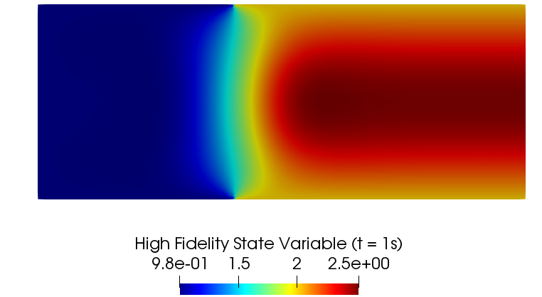
(a)

(b)

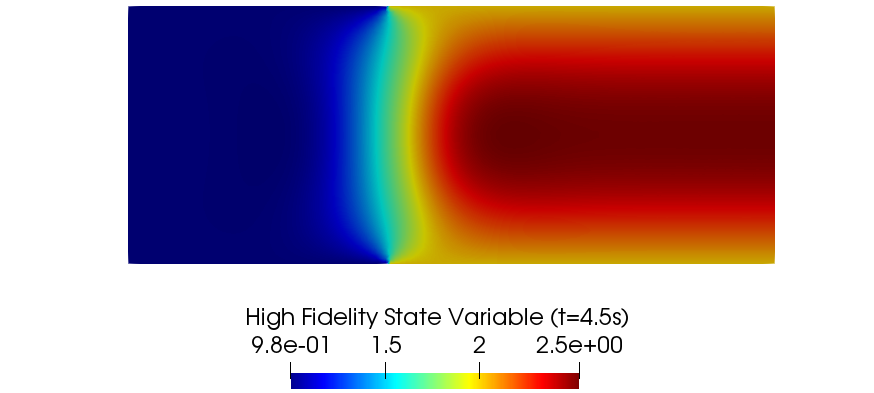
(c)

(d)

(e)

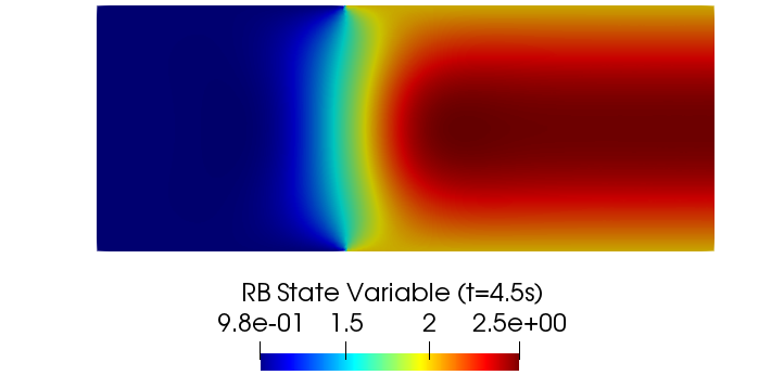
(f)

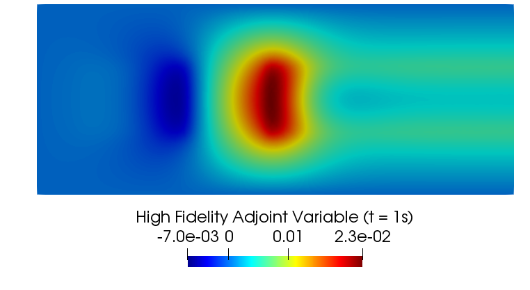
(g)

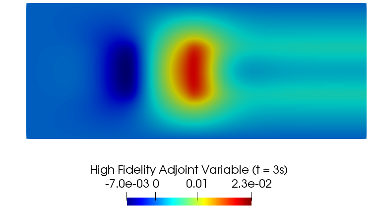
(h)

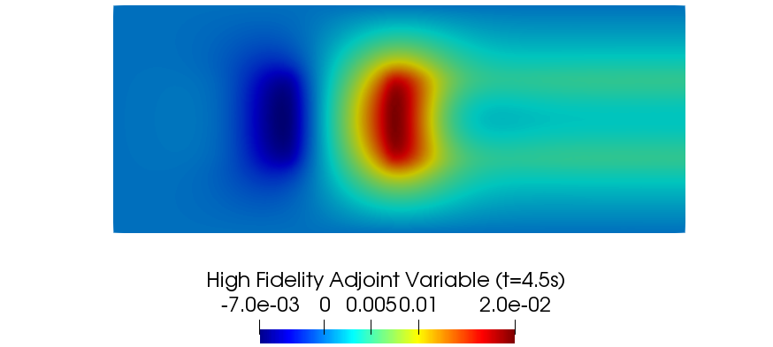
(i)

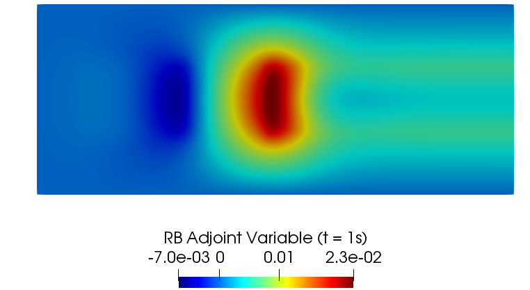
(j)

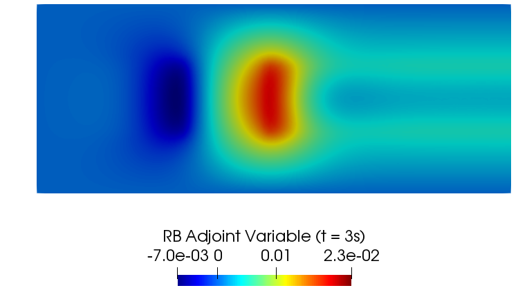
(k)

(l)

Figure 2. Optimal high fidelity and reduced solutions with $\alpha=0.01$ and $\boldsymbol{\mu}=(12.0,1.0,2.5)$. High fidelity state variable for $t=1s,3s,4.5s$ in (a), (b), (c), respectively, and reduced state variable for $t=1s,3s,4.5s$ in (d), (e), (f). Analogously, high fidelity adjoint variable in (f), (g), (h) and reduced adjoint variable in (i), (j), (k), for $t=1s,3s,4.5s.$

We decided to focus only on state and adjoint variable, since the control can be recovered through relation (12). The reduced model is able to reproduce the high fidelity solution for all the time instances considered. Furthermore, we propose a performance comparison with respect to the use of the Babuška inf-sup constant. Table 1 presents the average absolute and relative error

(72) $$\lVert e\rVert_{\text{abs}}{\;\vcentcolon=\;}\sqrt{(\lVert y^{\mathcal{N}}-y_{N}\rVert_{Y}^{2}+\lVert p^{\mathcal{N}}-p_{N}\rVert_{Y}^{2})}\quad\text{and}\quad\lVert e\rVert_{\text{rel}}{\;\vcentcolon=\;}\frac{\sqrt{(\lVert y^{\mathcal{N}}-y_{N}\rVert_{Y}^{2}+\lVert p^{\mathcal{N}}-p_{N}\rVert_{Y}^{2})}}{\sqrt{(\lVert y^{\mathcal{N}}\rVert_{Y}^{2}+\lVert p^{\mathcal{N}}\rVert_{Y}^{2})}},$$

together with the effectivity $\eta{\;\vcentcolon=\;}\Delta_{N}(\boldsymbol{\mu})/\lVert e\rVert_{\mathcal{Q}\times\mathcal{Q}}$ and the value of $\Delta_{N}(\boldsymbol{\mu})$. It is clear that the lower bound $\beta^{LB}(\boldsymbol{\mu})$ cannot give better results with respect to the exact computation of $\beta_{\mathcal{B}}^{{}^{\mathcal{N}}}(\boldsymbol{\mu})$. Still, exploiting the lower bound is of great convenience in the offline phase: indeed, the exact computation of the Babuška inf-sup constant for a given $\boldsymbol{\mu}$ takes, in average, $9.7s$, while the computation of the value of the lower bound is performed in $0.09s$. Furthermore, the use of the lower bound very mildly affects the accuracy, since the errors are comparable between the two considered options. An indicator of the effectivity of the new error bound is given also by Figure 3, where the value of the two constants are compared with respect $\mu_{1}$, which is the only parameter affecting the left hand side of the system. We have to remark that the value of the penalization parameter $\alpha$ drastically changes the tightness of the lower bound: for higher $\alpha$, we have a bad approximation of the Babuška inf-sup constant. This phenomenon is not new in literature, see, for example [24]. We can observe a good approximation of $\beta_{\mathcal{B}_{s}}^{N_{h}}$ in Figure 3(a), while we lose precision for smaller values of the penalization parameter as depicted in Figure 3(b).

Table 1. Unsteady case: performance analysis for the problem ($P$) for $\alpha=0.01$. Average error, estimators and effectivities exploiting the lower bound $\beta^{LB}(\boldsymbol{\mu})$ and the Babuška inf-sup constant $\beta_{\mathcal{B}}^{\mathcal{N}}(\boldsymbol{\mu})$, with respect to $N$.

$N$	$\beta^{LB}$				$\beta_{\mathcal{B}}^{\mathcal{N}}$
	$\lVert e\rVert_{\text{rel}}$	$\lVert e\rVert_{\text{abs}}$	$\Delta_{N}(\boldsymbol{\mu})$	$\eta$	$\lVert e\rVert_{\text{rel}}$	$\lVert e\rVert_{\text{abs}}$	$\Delta_{N}(\boldsymbol{\mu})$	$\eta$
1	5.61e–1	4.37e+0	1.29e+2	2.96e+1	5.25e–1	4.46e+1	1.30e+1	2.91e+0
3	1.81e–1	5.84e–1	3.42e+1	5.86e+1	1.16e–1	5.58e–1	3.16e+0	5.67e+0
5	3.13e–2	1.58e–1	7.25e+0	4.58e+1	3.84e–2	1.99e–1	9.03e–1	4.53e+0
7	1.12e–3	4.98e–2	3.07e–1	6.17e+1	7.70e–3	3.76e–2	1.98e–1	5.26e+0
9	4.36e–2	1.33e–2	6.38e–1	4.78e+1	3.42e–3	1.24e–2	5.41e–2	4.36e+0
11	1.46e–2	4.68e–3	2.23e–1	4.76e+1	1.19e–3	4.06e–3	2.11e–2	5.21e+0
13	3.90e–4	1.35e–3	7.32e–2	5.38e+1	3.53e–4	1.26e–3	6.46e–3	5.10e+0

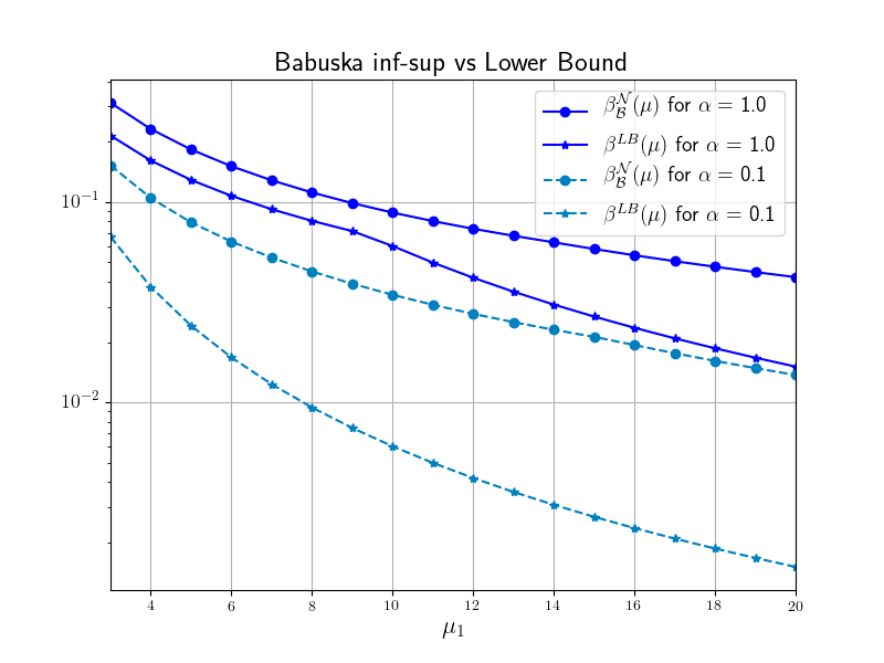
(a)

(b)

Figure 3. Comparison of the value of the lower bound $\beta^{LB}$ with respect to the exact Babuška inf-sup constant $\beta_{\mathcal{B}}^{\mathcal{N}}$ for $\alpha=1,0.1$ and $\alpha=0.01,0.001$ in (a) and (b), respectively. The analysis has been performed varying the value of $\mu_{1}$.

5.1.2. Steady Case

We report the results for the simulation of problem ($P_{s}$). The high fidelity problem has dimension $\mathcal{N}=N_{h}=9072$. We performed a greedy algorithm which reached the tolerance $\tau$ after picking $N=11$. In other words, the reduced system is much smaller with respect to the FE one, with a dimension of $4N=44$, after the aggregated space procedure. The number $N$ is lower compared to the time dependent case: this is not surprising considering the simpler context of a steady problem.
We fixed $\alpha=0.01$ and we propose a representative solution, obtained exploiting $\beta_{s}^{LB}$, in Figure 4 and an averaged performance analysis in Table 2. The latter shows the performance of the greedy considering approach with respect an average absolute and relative error, given by

(73) $$\lVert e\rVert_{\text{abs}}{\;\vcentcolon=\;}\sqrt{(\lVert y^{N_{h}}-y_{N}\rVert_{Y}^{2}+\lVert p^{N_{h}}-p_{N}\rVert_{Y}^{2})}\quad\text{and}\quad\lVert e\rVert_{\text{rel}}{\;\vcentcolon=\;}\frac{\sqrt{(\lVert y^{N_{h}}-y_{N}\rVert_{Y}^{2}+\lVert p^{N_{h}}-p_{N}\rVert_{Y}^{2})}}{\sqrt{(\lVert y^{N_{h}}\rVert_{Y}^{2}+\lVert p^{N_{h}}\rVert_{Y}^{2})}},$$

respectively. The analysis has been carried out with the use of the lower bound and the Babuška inf-sup constant and presents also a comparison of the effectivity value $\eta{\;\vcentcolon=\;}\Delta_{N}(\boldsymbol{\mu})/\lVert e\rVert_{Y\times Y}$ and the error estimator itself. As already specified for the time dependent test case, the lower bound cannot perform better with respect to the exact Babuška inf-sup constant. Indeed, the latter is preferable in terms of estimator and effectivity. Nonetheless, the lower bound gives comparable results in the average error analysis and we underline that exploiting $\beta^{LB}_{s}$ is computationally convenient also in the steady case. Indeed, the computation of $\beta_{s}^{LB}$ approximately takes 0.09s, while the eigenvalue problem associated to $\beta_{\mathcal{B}_{s}}^{N_{h}}$ is solved in $0.38s$ and we recall that the process must be repeated for the $N_{\text{max}}$ parameters of $\mathcal{P}_{h}$. In other words, employing the surrogate error estimator guarantees a faster offline phase, also for less complicated problems.

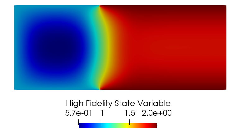
(a)

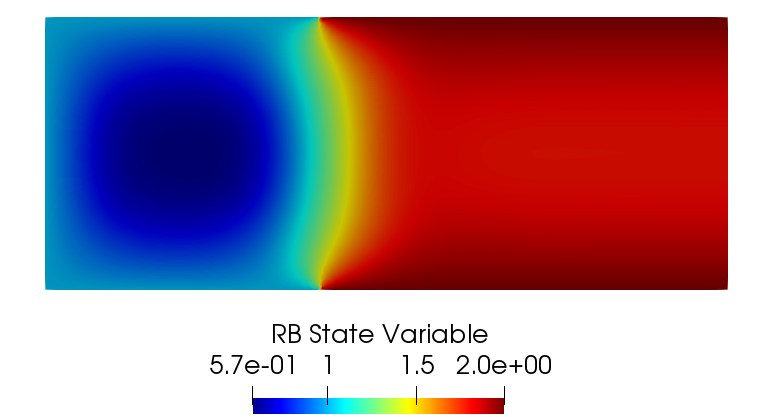
(b)

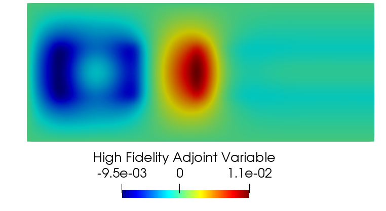
(c)

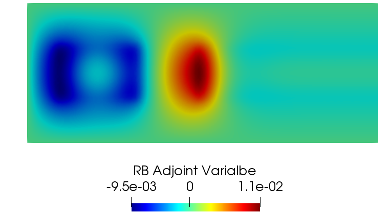
(d)

Figure 4. Optimal high fidelity and reduced solutions with $\alpha=0.01$ and $\boldsymbol{\mu}=(15.0,0.6,1.8)$. High fidelity state variable in (a) and reduced state variable in (b). Analogously, high fidelity adjoint variable in (c) and reduced adjoint variable in (d).

Furthermore, also in this case, the value of $\alpha$ highly influences the effectivity of the greedy procedure, as plots in Figure 5 show. If the value of $\alpha$ decreases, the effectivity increases, since the lower bound becomes a worse approximation of the Babuška inf-sup constant, as already observed in Section 5.1.1. A good approximation of $\beta_{\mathcal{B}_{s}}^{N_{h}}$ is shown in Figure 5(a), while we loose precision for smaller values of the penalization parameter as depicted in Figure 5(b). As in the time dependent case, we showed the comparison varying the value if $\mu_{1}$: indeed, the observation parameters $\mu_{2}$ and $\mu_{3}$, does not change the behaviour of the Babuška inf-sup since they only affect the right hand side of the optimality system. The behaviour of the constants is very similar to the unsteady ones. The main reason is in the space-time formulation itself, which presents almost the same structure of the simpler steady problem.
Finally, speaking about the computational time gain of the reduced framework, also in the steady case we can observe a quite important speedup, which is around $80,85$, independently from the value of $N$.

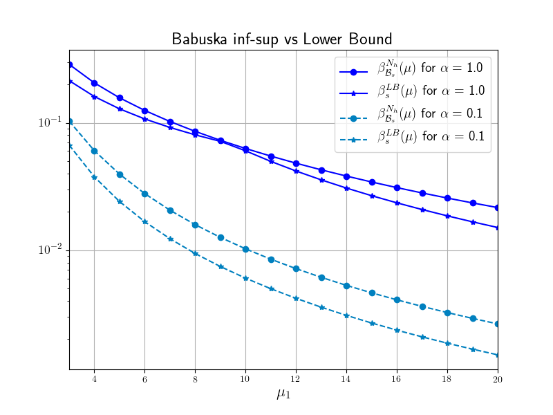
(a)

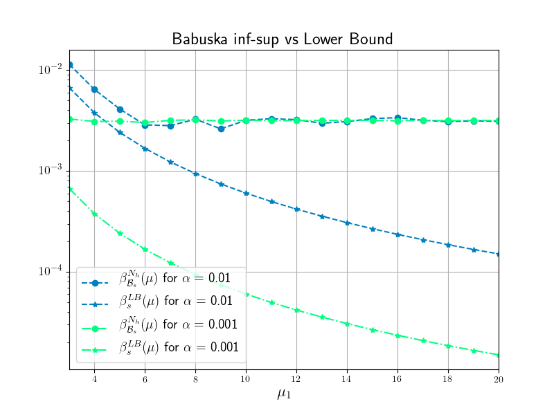
(b)

Figure 5. Comparison of the value of the lower bound $\beta^{LB}_{s}(\boldsymbol{\mu})$ with respect to the exact Babuška inf-sup constant $\beta_{\mathcal{B}_{s}}^{N_{h}}(\boldsymbol{\mu})$ for $\alpha=1,0.1$ and $\alpha=0.01,0.001$ in (a) and (b), respectively. The analysis has been performed varying the value of $\mu_{1}$.

Table 2. Steady case: performance analysis for the problem ($P_{s}$). Avarage error, estimators and effectivities exploiting the lower bound $\beta_{s}^{LB}$ and the Babuška inf-sup constant $\beta_{s}^{N_{h}}$, with respect to $N$.

$N$	$\beta^{LB}_{s}(\boldsymbol{\mu})$				$\beta_{\mathcal{B}_{s}}^{N_{h}}(\boldsymbol{\mu})$
	$\lVert e\rVert_{\text{rel}}$	$\lVert e\rVert_{\text{abs}}$	$\Delta_{N}(\boldsymbol{\mu})$	$\eta$	$\lVert e\rVert_{\text{rel}}$	$\lVert e\rVert_{\text{abs}}$	$\Delta_{N}(\boldsymbol{\mu})$	$\eta$
1	7.76e–1	6.08e–1	7.35e+1	1.20e+2	7.72e–1	5.57e–1	1.52e+1	2.73e+1
3	1.23e–1	4.85e–2	4.36e+1	1.75e+2	1.71e–1	5.56e–2	1.40e+0	2.52e+1
5	3.83e–2	1.77e–2	5.61e+0	1.86e+1	4.76e–2	1.84e–2	3.91e–1	2.11e+1
7	6.28e–3	1.92e–3	9.66e–1	2.11e+2	1.07e–2	3.52e–3	1.05e–1	2.98e+1
9	1.59e–3	6.64e–4	1.44e–1	1.56e+2	5.07e–3	1.36e–3	3.01e–2	2.21e+1
11	9.30e–4	2.18e–4	7.27e–2	1.51e+2	1.45e–3	2.19e–4	6.88e–3	3.14e+1

In the next Section we will show how the proposed lower bound performs in a more complex test case, where also geometrical parametrization is considered.

5.2. Physical and Geometrical Parametrization

In this Section we propose a boundary OCP($\boldsymbol{\mu}$)  governed by a Graetz flow with physical and geometrical parametrization. As paramter dependent domain, we consider $\Omega(\boldsymbol{\mu})$ depicted in Figure 6. In this case the observation domain is $\Omega_{\text{obs}}(\boldsymbol{\mu})=\Omega_{3}(\boldsymbol{\mu})\cup\Omega_{4}(\boldsymbol{\mu})$, where $\Omega_{1}$ is the unit square, $\Omega_{3}(\boldsymbol{\mu})=[1,1+\mu_{2}]\times[0.8,1]$, $\Omega_{4}(\boldsymbol{\mu})=[1,1+\mu_{2}]\times[0.,0.2]$, while $\Omega_{2}(\boldsymbol{\mu})=[1,1+\mu_{2}]\times[0.2,0.8]$. The control domian is given by $\Gamma_{C}(\boldsymbol{\mu})=[1,1+\mu_{2}]\times\{0\}\cup[1,1+\mu_{2}]\times\{1\}.$

Figure 6. Domain $\Omega$. Observation domain: $\Omega_{\text{obs}}(\boldsymbol{\mu})=\Omega_{3}(\boldsymbol{\mu})\cup\Omega_{4}(\boldsymbol{\mu})$, Control domain: $\Gamma_{C}(\boldsymbol{\mu})$ (red dashed line). Blue solid line: Dirichlet boundary conditions. The reference domain $\Omega$ is given by $\mu_{2}=1$.

The parameter is $\boldsymbol{\mu}{\;\vcentcolon=\;}(\mu_{1},\mu_{2},\mu_{3})\in\mathcal{P}=[6.0,20.0]\times[1.0,3.0]\times[0.5,3.0]$, where $\mu_{1}$, as the previous test case, represents the Péclet number, $\mu_{2}$ is a geometrical parameter which stretches the length of the right part of the domain, $\mu_{3}$ is a constant desired state $y_{d}$ observed in $\Omega_{\text{obs}}(\boldsymbol{\mu})$. Here, we control the Neumann conditions in order to achieved the desired observation. The problem reads as follows: given $\boldsymbol{\mu}\in\mathcal{P}$, find the pair $(y,p)\in\mathcal{Y}_{0}\times\mathcal{Y}_{T}$ such that

($$P^{g} \begin{cases}\displaystyle y\chi_{\Omega_{\text{obs}}(\boldsymbol{\mu})}-\frac{\partial p}{\partial t}-\frac{1}{\mu_{1}}\Delta p-x_{2}(1-x_{2})\frac{\partial p}{\partial x_{1}}=\mu_{3}\chi_{\Omega_{\text{obs}}(\boldsymbol{\mu})}&\text{ in }\Omega(\boldsymbol{\mu})\times[0,T],\\ \displaystyle\frac{\partial y}{\partial t}-\frac{1}{\mu_{1}}\Delta y-x_{2}(1-x_{2})\frac{\partial y}{\partial x_{1}}-\frac{1}{\alpha}p\chi_{\Omega_{u}}=0&\text{ in }\Omega(\boldsymbol{\mu})\times[0,T],\\ y(0)=y_{0}&\text{ in }\Omega(\boldsymbol{\mu}),\\ p(T)=0&\text{ in }\Omega(\boldsymbol{\mu}),\\ \displaystyle\frac{1}{\mu_{1}}\frac{\partial y}{\partial n}=0&\text{ on $\Gamma_{N}(\boldsymbol{\mu})\times[0,T],$}\\ \displaystyle\frac{1}{\mu_{1}}\frac{\partial y}{\partial n}=u&\text{ on $\Gamma_{C}(\boldsymbol{\mu})\times[0,T],$}\\ y=1\text{ and }p=0&\text{ on $\Gamma_{D}\times[0,T],$}\\ \end{cases}$$)

where $y_{0}=0$ in $\Omega(\boldsymbol{\mu})$ and satisfies the boundary conditions of the state variable, $\Gamma_{D}=\partial\Omega(\boldsymbol{\mu})\cap\{(x_{1},x_{2})\;|\;x_{1}\leq 1\}$ is the Dirichlet boundary domain, while $\Gamma_{N}(\boldsymbol{\mu})=\partial\Omega(\boldsymbol{\mu})\setminus\Gamma_{D}\cup\Gamma_{C}(\boldsymbol{\mu})$, is the Neumann boundary. Also for this case, we can focus our attention on the steady version, i.e.: given $\boldsymbol{\mu}\in\mathcal{P}$, find the pair $(y,p)\in Y\times Y$ such that

($$P_{s}^{g} \begin{cases}\displaystyle y-\frac{1}{\mu_{1}}\Delta p-x_{2}(1-x_{2})\frac{\partial p}{\partial x_{1}}=\mu_{3}\chi_{\Omega_{\text{obs}}(\boldsymbol{\mu})}&\text{ in }\Omega(\boldsymbol{\mu}),\\ \displaystyle-\frac{1}{\mu_{1}}\Delta y-x_{2}(1-x_{2})\frac{\partial y}{\partial x_{1}}-\frac{1}{\alpha}p=0&\text{ in }\Omega(\boldsymbol{\mu}),\vspace{2mm}\\ \displaystyle\frac{1}{\mu_{1}}\frac{\partial y}{\partial n}=0&\text{ on $\Gamma_{N}(\boldsymbol{\mu}),$}\\ \displaystyle\frac{1}{\mu_{1}}\frac{\partial y}{\partial n}=u&\text{ on $\Gamma_{C}(\boldsymbol{\mu}),$}\\ y=1\text{ and }=0&\text{ on $\Gamma_{D},$}\\ \end{cases}$$)

For this test case, since $\Omega_{\text{obs}}(\boldsymbol{\mu})\neq\Omega$, we decided to exploit the lower bound (69) for $\alpha=0.07$, both for the unsteady and the steady case, for consistency with respect to the previous test case. We analyzed also other values of the penalization parameters and the last bound of (68): we postpone the analysis in Remark 5. We will give the exact form of the involved quantities after the tracing back of the domain, since every step of the greedy algorithm is performed in the reference domain $\Omega$ given by $\mu_{2}=1$, the interested reader can find the details in [32]. We underline that the choice of the reference parameter affect the value of the constants $c_{u}$ and $c_{\text{obs}}$ but, for the sake of notation, we will omit the parameter dependency. In this case,

(74) $$\gamma_{a}(\boldsymbol{\mu}){\;\vcentcolon=\;}\min\left\{\frac{1}{\mu_{1}},\frac{1}{\mu_{1}\mu_{2}},\frac{\mu_{2}}{\mu_{1}},1\right\}\frac{1}{(1+C_{\Omega}^{2})},$$

where $C_{\Omega}$ is the Poincaré associated to the reference domain. Furthermore, we can give an explicit definition of $c_{u}=C_{\Gamma_{C}}$, i.e. the trace constant satisfying $\lVert p\rVert_{\Gamma_{C}}\leq C_{\Gamma_{C}}\lVert p\rVert_{H_{1}(\Omega)}$, once again we refer to [39]. We remark that the Poincaré and the trace constants can be evaluated directly through the resolution of an eigenvalue problem which has to be performed only once since defined in the reference domain $\Omega$. In other words, their exact computation does not impact the offline performance of the reduced space building procedure. Furthermore, following the same strategy of (71), we obtain that $c_{c}(\boldsymbol{\mu})=C_{\Gamma_{C}}$. For the space-time discretization we exploited $\mathbb{P}^{1}-\mathbb{P}^{1}$ elements and $N_{t}=30$ in the time interval $[0,T]=[0.,5.]$, i.e. $\Delta t=1./6.$, in order to compare our results with [46]. Also for this test case, we perform a greedy algorithm on $\mathcal{P}_{h}$ of cardinality $N_{\text{max}}=225$ picked through an uniform distribution on $\mathcal{P}$. The tolerance has been chosen as $\tau=1\cdot 10^{-4}$. For the steady and the unsteady case, we propose a performance analysis over $100$ parameters with a uniform distribution in $\mathcal{P}$. The results for the unsteady and the steady case follow.

5.2.1. Unsteady Case

This section deals with problem ($P^{g}$), with fixed $\alpha=0.07$, to which we applied the greedy algorithm using the lower bound (69). To achieve the tolerance $\tau$, the offline phase took $N=19$. Once again, exploiting the aggragated spaces strategy, we ended up with a reduced space of global dimension $4N=76$. The problem at hand, due to the boundary control and the geometrical parametrization, needs a greater number of basis with respect to the previous example. Still, the global reduced dimension is convenient compared to the high fidelity dimension $\mathcal{N}=N_{h}\times N_{t}=310980$. This is the reason we reach, also in this case, a good speed up around the value of $3\cdot 10^{4}$ for all $N$, obtained averaging over $100$ parameters uniformly distributed in $\mathcal{P}$. Figure 7 shows representative high fidelity and reduced state and adjoint solutions for $t=1s,3s,4.5s$, with $\alpha=0.07$ and $\boldsymbol{\mu}=(15.0,1.5,2.5)$. The reduced solutions recover the high-fidelity behaviour. The same is for the control variable, represented in Figure 8(a) for $x_{2}=1$ (we omitted $x_{2}=0$, due to the symmetry of the problem): the two solutions visually coincide for all the time instances.

Table 3. Unsteady case: performance analysis for the problem ($P^{g}$) for $\alpha=0.07$. Average error, estimators and effectivities exploiting the lower bound $\beta^{LB}(\boldsymbol{\mu})$ and the Babuška inf-sup constant $\beta_{\mathcal{B}}^{\mathcal{N}}(\boldsymbol{\mu})$, with respect to $N$.

$N$	$\beta^{LB}(\boldsymbol{\mu})$				$\beta_{\mathcal{B}}^{\mathcal{N}}(\boldsymbol{\mu})$
	$\lVert e\rVert_{\text{rel}}$	$\lVert e\rVert_{\text{abs}}$	$\Delta_{N}(\boldsymbol{\mu})$	$\eta$	$\lVert e\rVert_{\text{rel}}$	$\lVert e\rVert_{\text{abs}}$	$\Delta_{N}(\boldsymbol{\mu})$	$\eta$
1	5.61e–1	7.16e+0	3.05e+4	4.27e+3	6.62e–1	1.51e+1	7.68e+1	5.08e+1
3	2.10e–1	2.26e+0	5.44e+3	2.40e+3	2.75e–1	3.64e–1	1.96e+1	5.41e+1
5	8.66e–2	8.92e–1	1.99e+3	2.23e+3	8.01e–2	1.33e–1	3.89e+0	2.91e+1
7	3.88e–2	4.11e–1	6.79e+2	1.65e+3	4.57e–2	7.03e–2	3.89e+0	2.76e+1
9	2.46e–2	2.68e–1	4.99e+2	1.91e+3	2.17e–2	3.71e–2	1.94e+0	2.84e+1
11	1.09e–2	1.11e–1	1.95e+2	1.76e+3	9.06e–3	1.65e–2	1.05e+0	2.76e+1
13	7.16e–3	7.83e–2	1.40e+2	1.79e+3	5.98e–3	9.39e–3	4.59e–1	2.82e+1
15	4.60e–3	4.93e–2	1.08e+2	2.20e+3	4.26e–3	6.61e–3	2.65e–1	3.34e+1
17	2.48e–3	2.46e–2	4.65e+1	1.88e+3	2.36e–3	4.01e–3	1.11e–1	2.76e+1
19	1.72e–3	1.16e–2	3.14e+1	1.93e+3	1.73e–3	4.81e–3	6.97e–2	2.55e+1

The performance of the greedy algorithm is also evaluated in Table 3. It represents the average errors defined in (72) together with the effectivity and the error estimator with respect to the Babuška inf-sup constant $\beta_{\mathcal{B}}^{\mathcal{N}}(\boldsymbol{\mu})$ and the lower bound. In this case, we lose a lot in effectivity, but we recall that computing $225$ Babuška inf-sup constants is quite expensive compared to the evaluation of the value of $\beta^{LB}(\boldsymbol{\mu})$. Indeed, the first constant, in this case, takes around $8.6s$ to be computed, in average, while, as already said, $\beta^{LB}(\boldsymbol{\mu})$ is computed in $0.09s$.

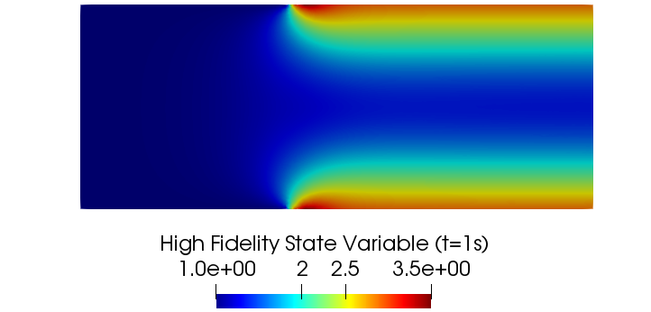
(a)

(b)

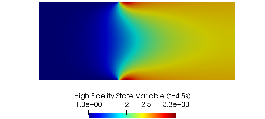
(c)

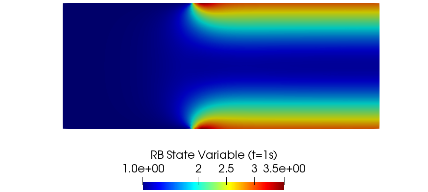
(d)

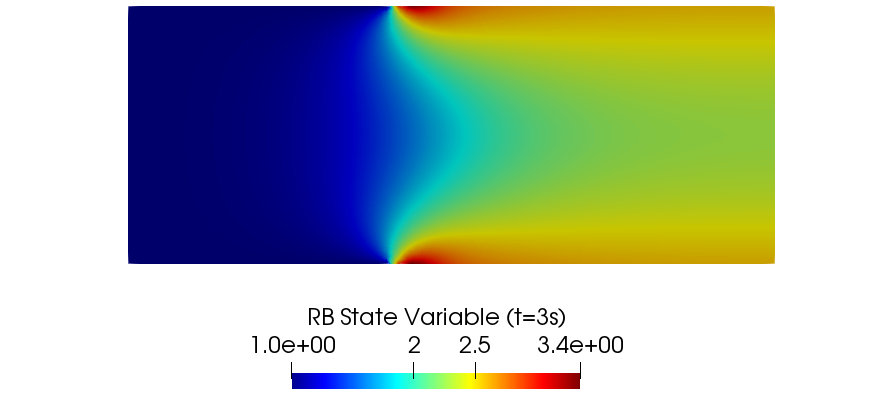
(e)

(f)

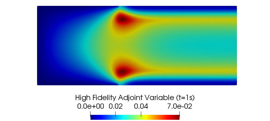
(g)

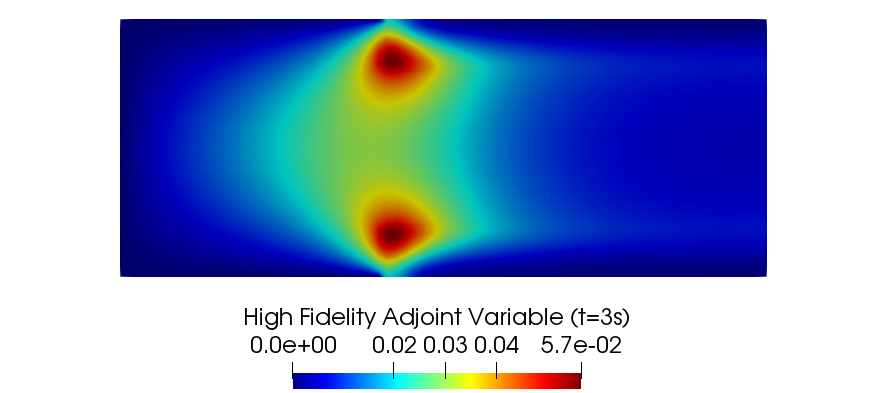
(h)

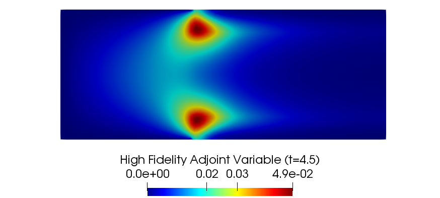
(i)

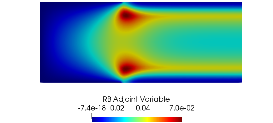
(j)

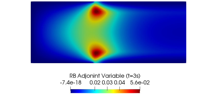
(k)

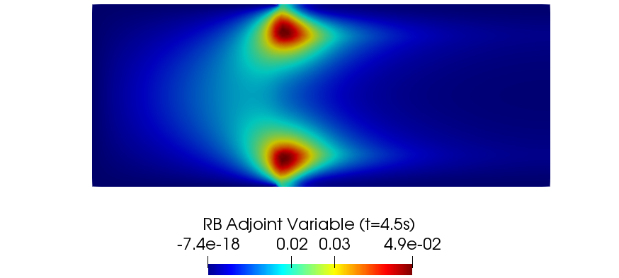
(l)

Figure 7. Optimal high fidelity and reduced steady control variables with $\alpha=0.07$ and $\boldsymbol{\mu}=(15.0,1.5,2.5)$. High fidelity state variable for $t=1s,3s,4.5s$ in (a), (b), (c), respectively, and reduced state variable for $t=1s,3s,4.5s$ in (d), (e), (f). Analogously, high fidelity adjoint variable in (f), (g), (h) and reduced adjoint variable in (i), (j), (k), for $t=1s,3s,4.5s.$

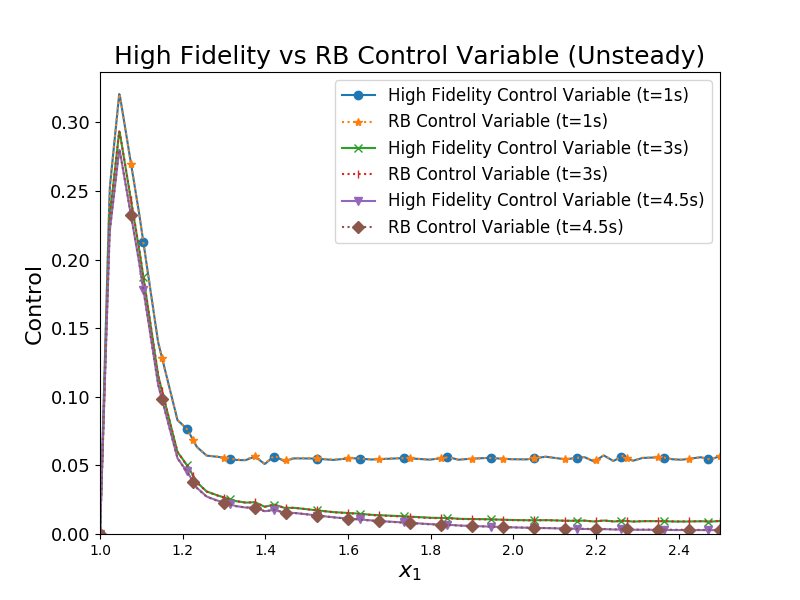
(a)

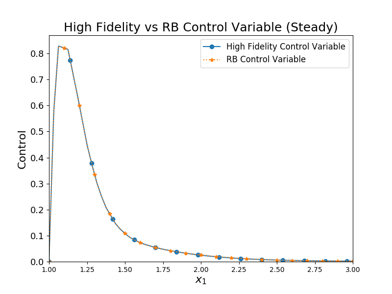
(b)

Figure 8. Optimal high fidelity and reduced control variable for the unsteady and steady case with $\alpha=0.07$. Unsteady: the solutions are presented for $t=1s,3s,4.5s$ and $\boldsymbol{\mu}=(15.0,1.5,2.5)$ in (a). Staedy: $\boldsymbol{\mu}=(12.0,2,2.5)$ in (b). In both cases the high fidelity and the reduced solutions coincide.

Furthermore, the relatives error of the two approaches (first and fifth columns of Table 3) are totally comparable. However, we can see how $\beta^{LB}(\boldsymbol{\mu})$ suffers the approximation in Figure 9, where the two constants are compared with respect to the value of $\mu_{1}$ for several values of $\alpha$, with $\mu_{2}=2$ fixed. In this case, the addition of the geometrical parametrization, influences the bound, which worsens not only for lower values of $\alpha$, but also for greater values of $\mu_{2}$, as we can observe from Figure 10.

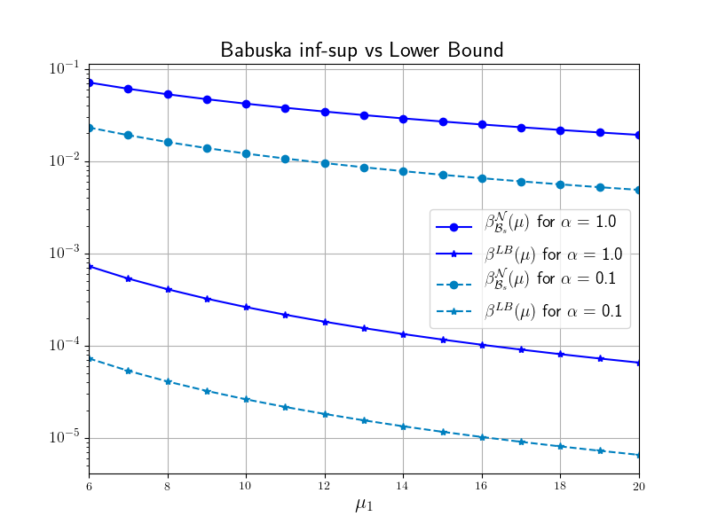
(a)

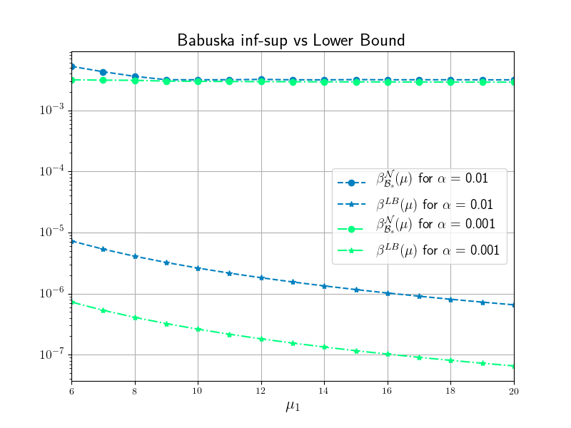
(b)

Figure 9. Comparison of the value of the lower bound $\beta^{LB}(\boldsymbol{\mu})$ with respect to the exact Babuška inf-sup constant $\beta_{\mathcal{B}}^{\mathcal{N}}(\boldsymbol{\mu})$ for $\alpha=1,0.1$ and $\alpha=0.01,0.001$ in (a) and (b), respectively. The analysis has been performed varying the value of $\mu_{1}$ and fixing $\mu_{2}=2$.

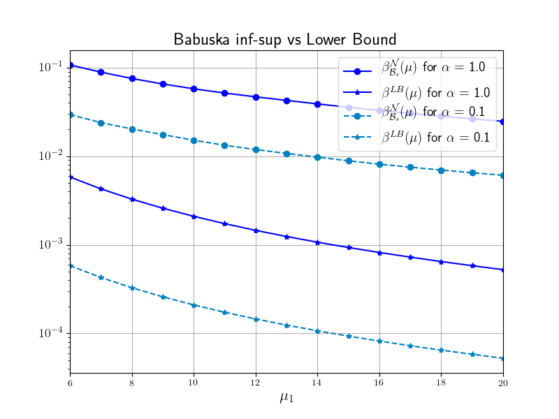
(a)

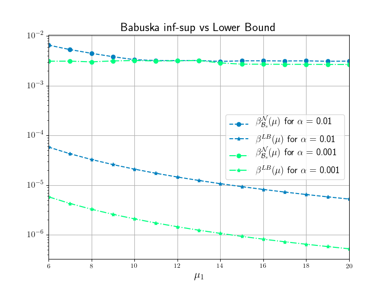
(b)

Figure 10. Comparison of the value of the lower bound $\beta^{LB}(\boldsymbol{\mu})$ with respect to the exact Babuška inf-sup constant $\beta_{\mathcal{B}}^{\mathcal{N}}(\boldsymbol{\mu})$ for $\alpha=1,0.1$ and $\alpha=0.01,0.001$ in (a) and (b), respectively. The analysis has been performed varying the value of $\mu_{1}$ and fixing $\mu_{2}=1$.

5.2.2. Steady Case

We briefly describe the performance of the lower bound $\beta^{LB}_{s}(\boldsymbol{\mu})$ for the problem ($P_{s}^{g}$). The problem with initial dimension of $\mathcal{N}=N_{h}=10366$ is reduced to $4N=40$. In Figure 11 we present some representative solutions for state and adjoint variable (the control is recovered through (12) and represented in Figure 8(b)) while an averaged performance analysis is considered in table Table 4, where errors (73) are shown, together with an effectivity and error estimator behaviours. Also in this case, in terms of effectivity, by definition, the Babuška inf-sup constant gives better results, but once again it pays in the offline basis construction, since the computation of the exact value $\beta^{N_{h}}_{\mathcal{B}_{s}}(\boldsymbol{\mu})$ take, averagely, $0.8s$. As in the time dependent, the effectivity is linked to the value of the penalization parameter as well as the value of $\mu_{2}$. For the sake of brevity we do not show the plots of the two constants varying $\alpha$ and $\mu_{1}$, since they are similar to Figure 9 and Figure 10. In terms of computational time needed for a reduced simulation, we reach a speed up of 135, averagely.

Table 4. Steady case: performance analysis for the problem ($P_{s}^{g}$). Avarage error, estimators and effectivities exploiting the lower bound $\beta_{s}^{LB}(\boldsymbol{\mu})$ and the Babuška inf-sup constant $\beta_{s}^{N_{h}}(\boldsymbol{\mu})$, with respect to $N$.

$N$	$\beta^{LB}_{s}(\boldsymbol{\mu})$				$\beta_{\mathcal{B}_{s}}^{N_{h}}(\boldsymbol{\mu})$
	$\lVert e\rVert_{\text{rel}}$	$\lVert e\rVert_{\text{abs}}$	$\Delta_{N}(\boldsymbol{\mu})$	$\eta$	$\lVert e\rVert_{\text{rel}}$	$\lVert e\rVert_{\text{abs}}$	$\Delta_{N}(\boldsymbol{\mu})$	$\eta$
2	3.16e–1	3.16e–1	3.25e+3	1.01e+4	5.82e–1	5.57e–1	1.01e+4	3.72e+1
4	5.69e–2	5.69e–2	4.53e+2	7.95e+3	6.67e–2	4.93e–2	7.95e+3	2.39e+1
6	1.52e–2	1.52e–2	1.11e+2	7.32e+3	2.72e–2	1.52e–2	7.32e+3	3.22e+1
8	5.23e–3	4.95e–3	3.40e+1	6.88e+3	7.33e–3	4.54e–3	6.88e+3	3.13e+1
10	2.03e–3	1.89e–3	1.25e+1	6.78e+3	4.63e–3	2.65e–3	6.78e+3	3.78e+1

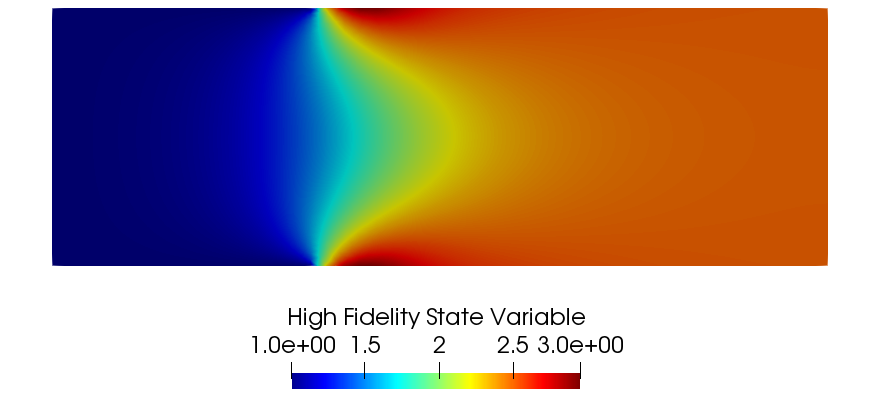
(a)

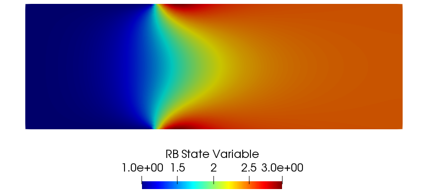
(b)

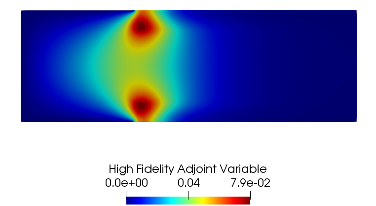
(c)

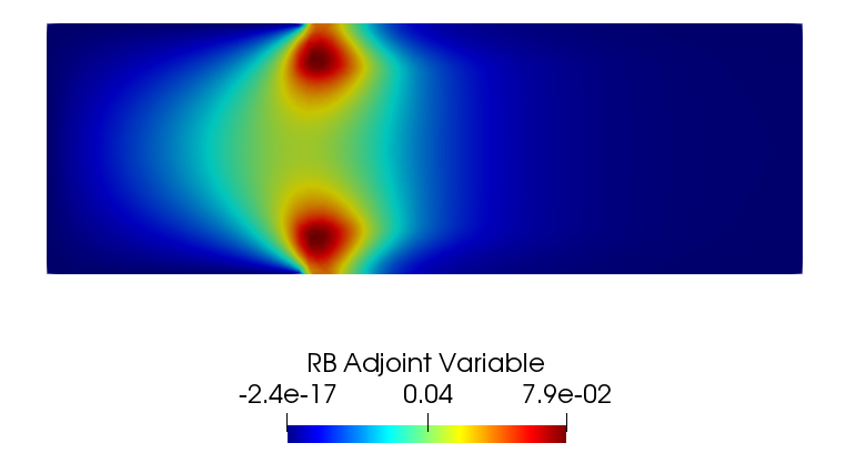
(d)

Figure 11. Optimal high fidelity and reduced solutions with $\alpha=0.07$ and $\boldsymbol{\mu}=(12.0,2.0,2.5)$. High fidelity state variable in (a) and reduced state variable in (b). Analogously, high fidelity adjoint variable in (c) and reduced adjoint variable in (d).

Remark 5 (Other $\alpha$, other $\beta^{LB}(\boldsymbol{\mu})$ ).

We performed other tests in the geometrical parametritazion. First of all, we tried several values of $\alpha$ and the results proved what is represented in Figures 9 and 10. Namely, the effectivity increases when $\alpha$ is smaller. We reached the value of $10^{5}$ with $\alpha=0.01,0.008$.
Furthermore, we tried to understand how the bound

(75) $$\beta^{LB}(\boldsymbol{\mu})=\beta_{s}^{LB}(\boldsymbol{\mu})=\displaystyle\frac{\gamma_{a}(\boldsymbol{\mu})}{\sqrt{2\max\left\{1,\left(\frac{c_{m}(\boldsymbol{\mu})c_{\text{obs}}}{\alpha\gamma_{a}(\boldsymbol{\mu})}\right)^{2}\right\}}},$$

performs with respect to (69). We recall that for this specific test case, we can use (75), since the control is not distributed. We still need to specify $c_{m}(\boldsymbol{\mu})$ and $c_{\text{obs}}$. It is easy to prove that $c_{m}(\boldsymbol{\mu})=C_{\Omega}\mu_{2}$. Then, both the constants can be approximated by an eigenvalue problem solved only once before the offline phase. Fixing $\alpha=0.07$, bound (75) performs better than (69), with lower effectivities both for steady and unsteady problem. All the results have been reported in Table 5. The values of $\beta^{LB}(\boldsymbol{\mu})$ must be compared to Table 3. We gain an order of magnitude for $\eta$ with the new bound. The same happens for $\beta^{LB}_{s}(\boldsymbol{\mu})$: indeed, compared with Table 4, we see that the new effectivities remains around $2\cdot 10^{3}$. For both the test case, the errors remain comparable. The better sharpness of (75), can be observe also in Figures 12, where the new lower bound and the Babuška inf-sup constant are depicted for $\alpha=0.07$ and $\mu_{2}=1$ (to be compared with Figure 10). Once again we reported only the time dependent case for the sake of brevity, since the steady case presents the same features.

Table 5. Unsteady case: performance analysis for the problem ($P^{g}$) and ($P_{s}^{g}$) for $\alpha=0.07$. Average error, estimators and effectivities exploiting the lower bounds $\beta^{LB}(\boldsymbol{\mu})$ and $\beta^{LB}_{s}(\boldsymbol{\mu})$ given by (75). (B.T.) Below tolerance $\tau$.

$N$	$\beta^{LB}(\boldsymbol{\mu})$				$\beta_{s}^{LB}(\boldsymbol{\mu})$
	$\lVert e\rVert_{\text{rel}}$	$\lVert e\rVert_{\text{abs}}$	$\Delta_{N}(\boldsymbol{\mu})$	$\eta$	$\lVert e\rVert_{\text{rel}}$	$\lVert e\rVert_{\text{abs}}$	$\Delta_{N}(\boldsymbol{\mu})$	$\eta$
2	4.23e–1	4.33e+0	3.689e+3	8.51e+2	2.99e–1	2.90e–1	6.53e+2	2.24e+3
4	1.45e–1	1.50e+0	1.01e+3	6.70e+2	6.36e–2	5.35e–2	1.12e+2	2.10e+3
6	5.24e–2	5.36e–1	2.67e+2	4.98e+2	3.01e–2	2.04e–2	3.99e+1	1.95e+3
8	2.80e–2	2.94e–1	1.58e+2	5.40e+2	7.60e–3	6.21e–3	2.56e+1	2.01e+3
10	1.38e–2	1.41e–1	6.83e+1	4.84e+2	B.T.
12	9.49e–3	9.21e–2	4.32e+1	4.69e+2	B.T.
14	5.12e–3	5.24e–2	3.01e+1	5.74e+2	B.T.
16	3.78e–3	3.85e–2	2.12e+1	5.52e+2	B.T.
18	2.57e–3	2.41e–2	1.52e+1	6.32e+2	B.T.
20	1.25e–3	1.21e–2	8.42e+0	6.93e+2	B.T.
22	9.07e–4	8.64e–3	6.30e+0	7.28e+2	B.T.

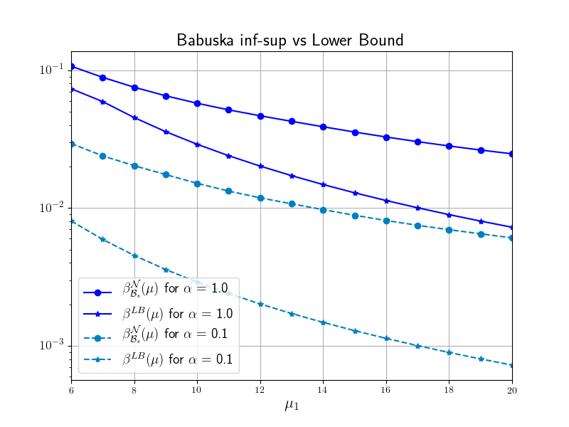
(a)

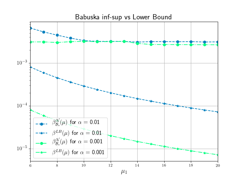
(b)

Figure 12. Comparison of the value of the lower bound (75) with respect to the exact Babuška inf-sup constant $\beta_{\mathcal{B}}^{\mathcal{N}}(\boldsymbol{\mu})$ for $\alpha=1,0.1$ and $\alpha=0.01,0.001$ in (a) and (b), respectively. The analysis has been performed varying the value of $\mu_{1}$ and fixing $\mu_{2}=1$.

6. Conclusions

In this work we presented a formulation for OCP($\boldsymbol{\mu}$)s governed by linear parabolic equations. We proposed a well-posedness analysis of the problem both at the continuous and at the discrete space-time level. We underline that classical discretization techniques may be too costly in order to deal with the task of optimization for several parameters. Then, we relied on greedy algorithm, extending the known literature of steady case to unsteady ones. The main novelty is given by the proposed new error bound, made by quantities which are known a priori. The strength of the bound is its great versatility, indeed it is valid for very general governing equations and control (from distributed to boundary ones). Furthermore, it is valid also for steady elliptic problems: at the best of our knowledge this is an improvement too, since the literature often relies on very expensive approximations algorithm [34]. At the space-time level, the proposed greedy algorithm not only assures a rapid and reliable online phase, but lightens the offline phase of such expensive problem formulation, which, to the best of our knowledge, was performed though standard Proper Orthogonal Decomposition approach [46]. The performance have been tested through a distributed OCP($\boldsymbol{\mu}$)  and a boundary OCP($\boldsymbol{\mu}$), with physical and geometrical parametrization. We reach high speed up values, due to the high-dimensionality of the all-at-once space-time OCP($\boldsymbol{\mu}$)s. This is a first step towards the applicability of ROM for OCP($\boldsymbol{\mu}$)s in very real-time context, where time evolution optimization is required.
Finally, we conclude with some perspectives related to the proposed estimator. First of all, the bound could be sharpened in order to achieve better results in terms of effectivities. A natural and interesting step could be the extension to more complicated state equations, like Stokes equations. This will enlarge the applicability of the greedy algorithm in space-time formulation in several fields: biomedical, industrial, environmental… Indeed, the main goal is to provide a very general tool to be used in real time contexts for different applications with the purpose of planning and management action.

References

- [1] RBniCS - reduced order modelling in FEniCS. https://www.rbnicsproject.org/, 2015.
- [2] I. Babuška. Error-bounds for finite element method. Numerische Mathematik, 16(4):322–333, Jan 1971.
- [3] E. Bader, M. Kärcher, M. A. Grepl, and K. Veroy. Certified reduced basis methods for parametrized distributed elliptic optimal control problems with control constraints. SIAM Journal on Scientific Computing, 38(6):A3921–A3946, 2016.
- [4] E. Bader, M. Kärcher, M. A. Grepl, and K. Veroy-Grepl. A certified reduced basis approach for parametrized linear-quadratic optimal control problems with control constraints. IFAC-PapersOnLine, 48(1):719–720, 2015.
- [5] F. Ballarin, E. Faggiano, A. Manzoni, A. Quarteroni, G. Rozza, S. Ippolito, C. Antona, and R. Scrofani. Numerical modeling of hemodynamics scenarios of patient-specific coronary artery bypass grafts. Biomechanics and Modeling in Mechanobiology, 16(4):1373–1399, Aug 2017.
- [6] D. Boffi, F. Brezzi, and M. Fortin. Mixed finite element methods and applications, volume 44. Springer-Verlag, Berlin and Heidelberg, 2013.
- [7] A. Buffa, Y. Maday, A. T. Patera, C. Prud’homme, and G. Turinici. A priori convergence of the greedy algorithm for the parametrized reduced basis method. ESAIM: Mathematical modelling and numerical analysis, 46(3):595–603, 2012.
- [8] J. C. de los Reyes and F. Tröltzsch. Optimal control of the stationary Navier-Stokes equations with mixed control-state constraints. SIAM Journal on Control and Optimization, 46(2):604–629, 2007.
- [9] L. Dedè. Optimal flow control for Navier-Stokes equations: Drag minimization. International Journal for Numerical Methods in Fluids, 55(4):347–366, 2007.
- [10] L. Dedè. Reduced basis method and a posteriori error estimation for parametrized linear-quadratic optimal control problems. SIAM Journal on Scientific Computing, 32(2):997–1019, 2010.
- [11] M. C. Delfour and J. Zolésio. Shapes and geometries: metrics, analysis, differential calculus, and optimization, volume 22. SIAM, Philadelphia, 2011.
- [12] A. L. Gerner and K. Veroy. Certified reduced basis methods for parametrized saddle point problems. SIAM Journal on Scientific Computing, 34(5):A2812–A2836, 2012.
- [13] S. Glas, A. Mayerhofer, and K. Urban. Two Ways to Treat Time in Reduced Basis Methods, pages 1–16. Springer International Publishing, Cham, 2017.
- [14] B. Haasdonk and M. Ohlberger. Reduced basis method for finite volume approximations of parametrized linear evolution equations. ESAIM: Mathematical Modelling and Numerical Analysis-Modélisation Mathématique et Analyse Numérique, 42(2):277–302, 2008.
- [15] J. Haslinger and R. A. E. Mäkinen. Introduction to shape optimization: theory, approximation, and computation. SIAM, Philadelphia, 2003.
- [16] J. S. Hesthaven, G. Rozza, and B. Stamm. Certified reduced basis methods for parametrized partial differential equations. SpringerBriefs in Mathematics, 2015, Springer, Milano.
- [17] M.L. Hinze, M. Köster, and S. Turek. A hierarchical space-time solver for distributed control of the Stokes equation. Technical Report, SPP1253-16-01, 2008.
- [18] M.L. Hinze, M. Köster, and S. Turek. A space-time multigrid method for optimal flow control. In Constrained optimization and optimal control for partial differential equations, pages 147–170. Springer, 2012.
- [19] M.L. Hinze, R. Pinnau, M. Ulbrich, and S. Ulbrich. Optimization with PDE constraints, volume 23. Springer Science & Business Media, Antwerp, 2008.
- [20] DBP Huynh, DJ Knezevic, Y Chen, Jan S Hesthaven, and AT Patera. A natural-norm successive constraint method for inf-sup lower bounds. Computer Methods in Applied Mechanics and Engineering, 199(29-32):1963–1975, 2010.
- [21] L. Iapichino, S. Trenz, and S. Volkwein. Reduced-order multiobjective optimal control of semilinear parabolic problems. In Bülent Karasözen, Murat Manguoğlu, Münevver Tezer-Sezgin, Serdar Göktepe, and Ömür Uğur, editors, Numerical Mathematics and Advanced Applications ENUMATH 2015, pages 389–397, Cham, 2016. Springer International Publishing.
- [22] L. Iapichino, S. Ulbrich, and S. Volkwein. Multiobjective pde-constrained optimization using the reduced-basis method. Adv. Comput. Math., 43(5):945–972, October 2017.
- [23] M. Kärcher and M. A. Grepl. A certified reduced basis method for parametrized elliptic optimal control problems. ESAIM: Control, Optimisation and Calculus of Variations, 20(2):416–441, 2014.
- [24] M. Kärcher, Z. Tokoutsi, M. A. Grepl, and K. Veroy. Certified reduced basis methods for parametrized elliptic optimal control problems with distributed controls. Journal of Scientific Computing, 75(1):276–307, 2018.
- [25] K. Kunisch and S. Volkwein. Proper orthogonal decomposition for optimality systems. ESAIM: Mathematical Modelling and Numerical Analysis, 42(1):1–23, 2008.
- [26] U. Langer, O. Steinbach, F. Tröltzsch, and H. Yang. Unstructured space-time finite element methods for optimal control of parabolic equations. 04 2020.
- [27] T. Lassila, A. Manzoni, A. Quarteroni, and G. Rozza. A reduced computational and geometrical framework for inverse problems in hemodynamics. International Journal for Numerical Methods in Biomedical Engineering, 29(7):741–776, 2013.
- [28] G. Leugering, P. Benner, S. Engell, A. Griewank, H. Harbrecht, M. Hinze, R. Rannacher, and S. Ulbrich. Trends in PDE constrained optimization. Springer, New York, 2014.
- [29] A. Logg, K.A. Mardal, and G. Wells. Automated Solution of Differential Equations by the Finite Element Method. Springer-Verlag, Berlin, 2012.
- [30] B. Mohammadi and O. Pironneau. Applied shape optimization for fluids. Oxford University Press, New York, 2010.
- [31] J. Nečas. Les méthodes directes en théorie des équations elliptiques. 1967.
- [32] F. Negri. Reduced basis method for parametrized optimal control problems governed by PDEs. Master thesis, Politecnico di Milano, 2011.
- [33] F. Negri, A. Manzoni, and G. Rozza. Reduced basis approximation of parametrized optimal flow control problems for the Stokes equations. Computers & Mathematics with Applications, 69(4):319–336, 2015.
- [34] F. Negri, G. Rozza, A. Manzoni, and A. Quarteroni. Reduced basis method for parametrized elliptic optimal control problems. SIAM Journal on Scientific Computing, 35(5):A2316–A2340, 2013.
- [35] M. Pošta and T. Roubíček. Optimal control of Navier–Stokes equations by Oseen approximation. Computers & Mathematics With Applications, 53(3):569–581, 2007.
- [36] C. Prud’Homme, D. V. Rovas, K. Veroy, L. Machiels, Y. Maday, A. Patera, and G. Turinici. Reliable real-time solution of parametrized partial differential equations: Reduced-basis output bound methods. Journal of Fluids Engineering, 124(1):70–80, 2002.
- [37] A. Quarteroni, G. Rozza, L. Dedè, and A. Quaini. Numerical approximation of a control problem for advection-diffusion processes. In IFIP Conference on System Modeling and Optimization, pages 261–273, Ceragioli F., Dontchev A., Futura H., Marti K., Pandolfi L. (eds) System Modeling and Optimization. CSMO 2005. vol 199. Springer, Boston, 2005.
- [38] A. Quarteroni, G. Rozza, and A. Quaini. Reduced basis methods for optimal control of advection-diffusion problems. In Advances in Numerical Mathematics, pages 193–216. RAS and University of Houston, Moscow, 2007.
- [39] A. Quarteroni and A. Valli. Numerical approximation of partial differential equations, volume 23. Springer Science & Business Media, Berlin and Heidelberg, 2008.
- [40] G. Rozza, D.B.P. Huynh, and A. Manzoni. Reduced basis approximation and a posteriori error estimation for Stokes flows in parametrized geometries: Roles of the inf-sup stability constants. Numerische Mathematik, 125(1):115–152, 2013.
- [41] G. Rozza, D.B.P. Huynh, and A.T. Patera. Reduced basis approximation and a posteriori error estimation for affinely parametrized elliptic coercive partial differential equations: Application to transport and continuum mechanics. Archives of Computational Methods in Engineering, 15(3):229–275, 2008.
- [42] Z. K. Seymen, H. Yücel, and B. Karasözen. Distributed optimal control of time-dependent diffusion–convection–reaction equations using space–time discretization. Journal of Computational and Applied Mathematics, 261:146–157, 2014.
- [43] M. Stoll and A. Wathen. All-at-once solution of time-dependent PDE-constrained optimization problems. 2010.
- [44] M. Stoll and A. Wathen. All-at-once solution of time-dependent Stokes control. J. Comput. Phys., 232(1):498–515, January 2013.
- [45] M. Strazzullo, F. Ballarin, R. Mosetti, and G. Rozza. Model reduction for parametrized optimal control problems in environmental marine sciences and engineering. SIAM Journal on Scientific Computing, 40(4):B1055–B1079, 2018.
- [46] M. Strazzullo, F. Ballarin, and G. Rozza. Pod–galerkin model order reduction for parametrized time dependent linear quadratic optimal control problems in saddle point formulation. Journal of Scientific Computing, 83(3):55, 2020.
- [47] M. Strazzullo, F. Ballarin, and G. Rozza. POD-Galerkin model order reduction for parametrized nonlinear time dependent optimal flow control: an application to Shallow Water Equations. Submitted, arXiv:2003.09695, 2020.
- [48] M. Strazzullo, Z. Zainib, F. Ballarin, and G. Rozza. Reduced order methods for parametrized nonlinear and time dependent optimal flow control problems: towards applications in biomedical and environmental sciences. In ENUMATH2019 proceedings, 2020.
- [49] K. Urban and A. T. Patera. A new error bound for reduced basis approximation of parabolic partial differential equations. Comptes Rendus Mathematique, 350(3-4):203–207, 2012.
- [50] Jinchao Xu and Ludmil Zikatanov. Some observations on Babuška and Brezzi theories. Numerische Mathematik, 94(1):195–202, 2003.
- [51] M. Yano. A space-time Petrov–Galerkin certified reduced basis method: Application to the Boussinesq equations. SIAM Journal on Scientific Computing, 36(1):A232–A266, 2014.
- [52] M. Yano, A. T. Patera, and K. Urban. A space-time hp-interpolation-based certified reduced basis method for Burgers’ equation. Mathematical Models and Methods in Applied Sciences, 24(09):1903–1935, 2014.
- [53] Z. Zainib, F. Ballarin, S. Fremes, P. Triverio, L. Jiménez-Juan, and G. Rozza. Reduced order methods for parametric optimal flow control in coronary bypass grafts, towards patient-specific data assimilation. International Journal for Numerical Methods in Biomedical Engineering, 2020.