Geometry of the symplectic Stiefel manifold endowed with the Euclidean metric

Abstract

The symplectic Stiefel manifold, denoted by $\mathrm{Sp}(2p,2n)$, is the set of linear symplectic maps between the standard symplectic spaces $\mathbb{R}^{2p}$ and $\mathbb{R}^{2n}$. When $p=n$, it reduces to the well-known set of $2n\times 2n$ symplectic matrices. We study the Riemannian geometry of this manifold viewed as a Riemannian submanifold of the Euclidean space $\mathbb{R}^{2n\times 2p}$. The corresponding normal space and projections onto the tangent and normal spaces are investigated. Moreover, we consider optimization problems on the symplectic Stiefel manifold. We obtain the expression of the Riemannian gradient with respect to the Euclidean metric, which then used in optimization algorithms. Numerical experiments on the nearest symplectic matrix problem and the symplectic eigenvalue problem illustrate the effectiveness of Euclidean-based algorithms.

1 Introduction

Let $J_{2m}$ denote the nonsingular and skew-symmetric matrix $\left[\begin{smallmatrix}0&I_{m}\\ -I_{m}&0\end{smallmatrix}\right]$, where $I_{m}$ is the $m\times m$ identity matrix and $m$ is any positive integer. The symplectic Stiefel manifold, denoted by

$$\mathrm{Sp}(2p,2n):=\left\{X\in\mathbb{R}^{2n\times 2p}:X^{\top}J_{2n}X=J_{2p}\right\},$$

is a smooth embedded submanifold of the Euclidean space $\mathbb{R}^{2n\times 2p}$ ($p\leq n$)  [12, Proposition 3.1]. We remove the subscript of $J_{2m}$ and $I_{m}$ for simplicity if there is no confusion. This manifold was studied in [12]: it is closed and unbounded; it has dimension $4np-p(2p-1)$; when $p=n$, it reduces to the symplectic group, denoted by $\mathrm{Sp}(2n)$. When $X\in\mathrm{Sp}(2p,2n)$, it is termed as a symplectic matrix.

Symplectic matrices are employed in many fields. They are indispensable for finding eigenvalues of (skew-)Hamiltonian matrices [4, 5, 6] and for model order reduction of Hamiltonian systems [16, 9]. They appear in Williamson’s theorem and the formulation of symplectic eigenvalues of symmetric and positive-definite matrices [19, 7, 14, 17]. Moreover, symplectic matrices can be found in the study of optical systems [11] and the optimal control of quantum symplectic gates [21]. Specifically, some applications can be reformulated as optimization problems on the set of symplectic matrices [16, 17].

In recent decades, most of studies on the symplectic topic focused on the symplectic group ($p=n$) including geodesics of the symplectic group [10], optimality conditions for optimization problems on the symplectic group [15, 20, 8], and optimization algorithms on the symplectic group [11, 18]. However, there was less attention to the geometry of the symplectic Stiefel manifold $\mathrm{Sp}(2p,2n)$. More recently, the Riemannian structure of $\mathrm{Sp}(2p,2n)$ was investigated in [12] by endowing it with a new class of metrics called canonical-like. This canonical-like metric is different from the standard Euclidean metric (the Frobenius inner product in the ambient space $\mathbb{R}^{2n\times 2p}$)

$$\left\langle X,Y\right\rangle:=\operatorname*{tr}(X^{\top}Y)\quad\mbox{for}~{}X,Y\in\mathbb{R}^{2n\times 2p},$$

where $\operatorname*{tr}(\,\cdot\,)$ is the trace operator. A priori reasons to investigate the Euclidean metric on $\mathrm{Sp}(2p,2n)$ are that it is arguably the most natural choice, and that there are specific applications with close links to the Euclidean metric, e.g., the projection onto $\mathrm{Sp}(2p,2n)$ with respect to the Frobenius norm (also known as the nearest symplectic matrix problem)

$$\min\limits_{X\in\mathrm{Sp}(2p,2n)}\left\|X-A\right\|^{2}_{\mathrm{F}}.$$ (1)

Note that this problem does not admit a known closed-form solution for general $A\in\mathbb{R}^{2n\times 2p}$.

In this paper, we consider the symplectic Stiefel manifold $\mathrm{Sp}(2p,2n)$ as a Riemannian submanifold of the Euclidean space $\mathbb{R}^{2n\times 2p}$. Specifically, the normal space and projections onto the tangent and normal spaces are derived. As an application, we obtain the Riemannian gradient of any function on $\mathrm{Sp}(2p,2n)$ in the sense of the Euclidean metric. Numerical experiments on the nearest symplectic matrix problem and the symplectic eigenvalue problem are reported. In addition, numerical comparisons with the canonical-like metric are also presented. We observe that the Euclidean-based optimization methods need fewer iterations than the methods with the canonical-like metric on the nearest symplectic problem, and Cayley-based methods perform best among all the choices.

The rest of paper is organized as follows. In section 2, we study the Riemannian geometry of the symplectic Stiefel manifold endowed with the Euclidean metric. This geometry is further applied to optimization problems on the manifold in section 3. Numerical results are presented in section 4.

2 Geometry of the Riemannian submanifold $\mathrm{Sp}(2p,2n)$

In this section, we study the Riemannian geometry of $\mathrm{Sp}(2p,2n)$ equipped with the Euclidean metric.

Given $X\in\mathrm{Sp}(2p,2n)$, let $X_{\perp}\in\mathbb{R}^{2n\times(2n-2p)}$ be a full-rank matrix such that $\operatorname*{span}(X_{\perp})$ is the orthogonal complement of $\operatorname*{span}(X)$. Then the matrix $\left[XJ\,\,\,JX_{\perp}\right]$ is nonsingular, and every matrix $Y\in\mathbb{R}^{2n\times 2p}$ can be represented as $Y=XJW+JX_{\perp}K$, where $W\in\mathbb{R}^{2p\times 2p}$ and $K\in\mathbb{R}^{(2n-2p)\times 2p}$; see [12, Lemma 3.2]. The tangent space of $\mathrm{Sp}(2p,2n)$ at $X$, denoted by ${\mathrm{T}_{X}}\mathrm{Sp}(2p,2n)$, is given by [12, Proposition 3.3]

$${\mathrm{T}_{X}}\mathrm{Sp}(2p,2n) =\{XJW+JX_{\perp}K:W\in{\cal S}_{\mathrm{sym}}(2p),K\in\mathbb{R}^{(2n-2p)\times 2p}\}$$ (2a)

$$=\{SJX:S\in{\cal S}_{\mathrm{sym}}(2n)\},$$ (2b)

where ${\cal S}_{\mathrm{sym}}(2p)$ denotes the set of all $2p\times 2p$ real symmetric matrices. These two expressions can be regarded as different parameterizations of the tangent space.

Now we consider the Euclidean metric. Given any tangent vectors $Z_{i}=XJW_{i}+JX_{\perp}K_{i}$ with $W_{i}\in{\cal S}_{\mathrm{sym}}(2p)$ and $K_{i}\in\mathbb{R}^{(2n-2p)\times 2p}$ for $i=1,2$, the standard Euclidean metric is defined as

$$g_{\mathrm{e}}(Z_{1},Z_{2}) :=\left\langle Z_{1},Z_{2}\right\rangle=\operatorname*{tr}(Z_{1}^{\top}Z_{2})$$

$$~{}=\operatorname*{tr}(W_{1}^{\top}J^{\top}X^{\top}XJW_{2})+\operatorname*{tr}(K_{1}^{\top}X^{\top}_{\perp}X_{\perp}K_{2})$$

$$\quad+\operatorname*{tr}(W_{1}^{\top}J^{\top}X^{\top}JX_{\perp}K_{2})+\operatorname*{tr}(K_{1}^{\top}X^{\top}_{\perp}J^{\top}XJW_{2}).$$

In contrast with the canonical-like metric proposed in [12]

$$g_{\rho,X_{\perp}}(Z_{1},Z_{2}) :={\frac{1}{\rho}\,\operatorname*{tr}}(W_{1}^{\top}W_{2})+\operatorname*{tr}(K_{1}^{\top}K_{2})\quad\text{with~{}}\rho>0,$$

$g_{\mathrm{e}}$ has cross terms between $W$ and $K$. Note that $g_{\mathrm{e}}$ is also well-defined when it is extended to $\mathbb{R}^{2n\times 2p}$. Then the normal space of $\mathrm{Sp}(2p,2n)$ with respect to $g_{\mathrm{e}}$ can be defined as

$$\left({\mathrm{T}_{X}}\mathrm{Sp}(2p,2n)\right)^{\perp}_{\mathrm{e}}:=\left\{N\in\mathbb{R}^{2n\times 2p}:g_{\mathrm{e}}(N,Z)=0\mbox{~{}for all~{}}Z\in{\mathrm{T}_{X}}\mathrm{Sp}(2p,2n)\right\}.$$

We obtain the following expression of the normal space.

Proposition 1.

Given $X\in\mathrm{Sp}(2p,2n)$, we have

$$\left({\mathrm{T}_{X}}\mathrm{Sp}(2p,2n)\right)^{\perp}_{\mathrm{e}}=\left\{JX\varOmega:\varOmega\in{\cal S}_{\mathrm{skew}}(2p)\right\},$$ (3)

where ${\cal S}_{\mathrm{skew}}(2p)$ denotes the set of all $2p\times 2p$ real skew-symmetric matrices.

Proof.

Given any $N=JX\varOmega$ with $\varOmega\in{\cal S}_{\mathrm{skew}}(2p)$, and $Z=XJW+JX_{\perp}K\in{\mathrm{T}_{X}}\mathrm{Sp}(2p,2n)$ with $W\in{\cal S}_{\mathrm{sym}}(2p)$, we have $g_{\mathrm{e}}(N,Z)=\operatorname*{tr}(N^{\top}Z)=\operatorname*{tr}(\varOmega^{\top}W)=0$, where the last equality follows from $\varOmega^{\top}=-\varOmega$ and $W^{\top}=W$. Therefore, it yields $N\in\left({\mathrm{T}_{X}}\mathrm{Sp}(2p,2n)\right)^{\perp}_{\mathrm{e}}$. Counting dimensions of ${\mathrm{T}_{X}}\mathrm{Sp}(2p,2n)$ and the subspace $\left\{JX\varOmega:\varOmega\in{\cal S}_{\mathrm{skew}}(2p)\right\}$, i.e., $4np-p(2p-1)$ and $p(2p-1)$, respectively, the expression (3) holds. ∎

Notice that $\left({\mathrm{T}_{X}}\mathrm{Sp}(2p,2n)\right)^{\perp}_{\mathrm{e}}$ is different from the normal space with respect to the canonical-like metric $g_{\rho,X_{\perp}}$, denoted by $\left({\mathrm{T}_{X}}\mathrm{Sp}(2p,2n)\right)^{\perp}$, which has the expression $\left\{XJ\varOmega:\varOmega\in{\cal S}_{\mathrm{skew}}(2p)\right\}$, obtained in [12].

The following proposition provides explicit expressions for the orthogonal projection onto the tangent and normal spaces with respect to the metric $g_{\mathrm{e}}$, denoted by $\left(\mathcal{P}_{X}\right)_{\mathrm{e}}$ and $\left(\mathcal{P}_{X}\right)_{\mathrm{e}}^{\perp}$, respectively.

Proposition 2.

Given $X\in\mathrm{Sp}(2p,2n)$ and $Y\in\mathbb{R}^{2n\times 2p}$, we have

$$\left(\mathcal{P}_{X}\right)_{\mathrm{e}}(Y) =Y-JX{\varOmega_{X,Y}},$$ (4)

$$\left(\mathcal{P}_{X}\right)_{\mathrm{e}}^{\perp}(Y) =JX{\varOmega_{X,Y}},$$ (5)

where ${\varOmega_{X,Y}}\in{\cal S}_{\mathrm{skew}}(2p)$ is the unique solution of the Lyapunov equation with unknown $\varOmega$

$$X^{\top}X\varOmega+\varOmega X^{\top}X=2\operatorname*{skew}(X^{\top}J^{\top}Y)$$ (6)

and $\operatorname*{skew}(A):=\frac{1}{2}(A-A^{\top})$ denotes the skew-symmetric part of $A$.

Proof.

For any $Y\in\mathbb{R}^{2n\times 2p}$, in view of (2a) and (3), it follows that

$$\left(\mathcal{P}_{X}\right)_{\mathrm{e}}(Y)=XJW_{Y}+JX_{\perp}K_{Y},\qquad\left(\mathcal{P}_{X}\right)_{\mathrm{e}}^{\perp}(Y)=JX\varOmega,$$

with $W_{Y}\in{\cal S}_{\mathrm{sym}}(2p)$, $K_{Y}\in\mathbb{R}^{(2n-2p)\times 2p}$ and $\varOmega\in{\cal S}_{\mathrm{skew}}(2p)$. Further, $Y$ can be represented as

$$Y=\left(\mathcal{P}_{X}\right)_{\mathrm{e}}(Y)+\left(\mathcal{P}_{X}\right)_{\mathrm{e}}^{\perp}(Y)=XJW_{Y}+JX_{\perp}K_{Y}+JX\varOmega.$$

Multiplying this equation from the left with $X^{\top}J^{\top}$, it follows that

$$X^{\top}J^{\top}Y=W_{Y}+X^{\top}X\varOmega.$$

Subtracting from this equation its transpose and taking into account that $W^{\top}=W$ and $\varOmega^{\top}=-\varOmega$, we get the Lyapunov equation (6) with unknown $\varOmega$. Since $X^{\top}X$ is symmetric positive definite, all its eigenvalues are positive, and, hence, equation (6) has a unique solution $\varOmega_{X,Y}$; see [13, Lemma 7.1.5]. Therefore, the relation (5) holds. Finally, (4) follows from $\left(\mathcal{P}_{X}\right)_{\mathrm{e}}(Y)=Y-\left(\mathcal{P}_{X}\right)_{\mathrm{e}}^{\perp}(Y)$. ∎

(a) Canonical-like metric

(b) Euclidean metric

Figure 1: Normal spaces and projections associated with different metrics on $\mathcal{M}=\mathrm{Sp}(2p,2n)$

Figure 1 illustrates the difference of the normal spaces and projections for the canonical-like metric $g_{\rho,X_{\perp}}$ and the Euclidean metric $g_{\mathrm{e}}$. Note that projections with respect to the canonical-like metric only require matrix additions and multiplications (see [12, Proposition 4.3]) while one has to solve the Lyapunov equation (6) in the Euclidean case.

The Lyapunov equation (6) can be solved using the Bartels–Stewart method [3]. Observe that the coefficient matrix $X^{\top}X$ is symmetric positive definite, and, hence, it has an eigenvalue decomposition $X^{\top}X=Q\Lambda Q^{\top}$, where $Q\in\mathbb{R}^{2p\times 2p}$ is orthogonal and $\Lambda=\operatorname*{diag}(\lambda_{1},\ldots,\lambda_{2p})$ is diagonal with $\lambda_{i}>0$ for $i=1,\ldots,2p$. Inserting this decomposition into (6) and multiplying it from the left and right with $Q^{\top}$ and $Q$, respectively, we obtain the equation

$$\Lambda U+U\Lambda=R$$

with $R=2Q^{\top}\mathrm{skew}(X^{\top}JY)Q$ and unknown $U=Q^{\top}\varOmega Q$. The entries of $U$ can then be computed as

$$u_{ij}=\dfrac{r_{ij}}{\lambda_{i}+\lambda_{j}},\quad i,j=1,\ldots,2p.$$

Finally, we find $\Omega=QUQ^{\top}$. The computational cost for matrix-matrix multiplications involved to generate (6) is $O(np^{2})$, and $O(p^{3})$ for solving this equation.

3 Application to Optimization

In this section, we consider a continuously differentiable real-valued function $f$ on $\mathrm{Sp}(2p,2n)$ and optimization problems on the manifold.

The Riemannian gradient of $f$ at $X\in\mathrm{Sp}(2p,2n)$ with respect to the metric $g_{\mathrm{e}}$, denoted by $\mathrm{grad}_{\mathrm{e}}f(X)$, is defined as the unique element of ${\mathrm{T}_{X}}\mathrm{Sp}(2p,2n)$ that satisfies the condition $g_{\mathrm{e}}\left(\mathrm{grad}_{\mathrm{e}}f(X),Z\right)=\mathrm{D}\bar{f}(X)[Z]$ for all $Z\in{\mathrm{T}_{X}}\mathrm{Sp}(2p,2n)$, where $\bar{f}$ is a smooth extension of $f$ around $X$ in $\mathbb{R}^{2n\times 2p}$, and $\mathrm{D}\bar{f}(X)$ denotes the Fréchet derivative of $\bar{f}$ at $X$. Since $\mathrm{Sp}(2p,2n)$ is endowed with the Euclidean metric, the Riemannian gradient can be readily computed by using [1, Section 3.6] as follows.

Proposition 3.

The Riemannian gradient of a function $f:\mathrm{Sp}(2p,2n)\to\mathbb{R}$ with respect to the Euclidean metric $g_{\mathrm{e}}$ has the following form

$$\mathrm{grad}_{\mathrm{e}}f(X)=\left(\mathcal{P}_{X}\right)_{\mathrm{e}}(\nabla\bar{f}(X))=\nabla\bar{f}(X)-JX\varOmega_{X},$$ (7)

where $\varOmega_{X}\in{\cal S}_{\mathrm{skew}}(2p)$ is the unique solution of the Lyapunov equation with unknown $\varOmega$

$$X^{\top}X\varOmega+\varOmega X^{\top}X=2\operatorname*{skew}\left(X^{\top}J^{\top}\nabla\bar{f}(X)\right),$$

and $\nabla\bar{f}(X)$ denotes the (Euclidean, i.e., classical) gradient of $\bar{f}$ at $X$.

In the case of the symplectic group $\mathrm{Sp}(2n)$, the Riemannian gradient (7) is equivalent to the formulation in [8], where the minimization problem was treated as a constrained optimization problem in the Euclidean space. We notice that $\varOmega_{X}$ in (7) is actually the Lagrangian multiplier of the symplectic constraints; see [8].

Expression (7) can be rewritten in the parameterization (2a): it follows from [12, Lemma 3.2] that

$$\mathrm{grad}_{\mathrm{e}}f(X)=XJW_{X}+JX_{\perp}K_{X}$$

with $W_{X}=X^{\top}J^{\top}\mathrm{grad}_{\mathrm{e}}f(X)$ and $K_{X}=\left(X^{\top}_{\perp}JX_{\perp}\right)^{-1}X^{\top}_{\perp}\mathrm{grad}_{\mathrm{e}}f(X)$. Moreover, for the purpose of using the Cayley retraction [12, Definition 5.2], it is essential to rewrite (7) in the parameterization (2b) with $S$ in a factorized form as in [12, Proposition 5.4]. To this end, observe that (7) is its own tangent projection and use the tangent projection formula of [12, Proposition 4.3] to obtain

$$\mathrm{grad}_{\mathrm{e}}f(X)=S_{X}JX$$

with $S_{X}=G_{X}\mathrm{grad}_{\mathrm{e}}f(X)(XJ)^{\top}+XJ(G_{X}\mathrm{grad}_{\mathrm{e}}f(X))^{\top}$ and $G_{X}=I-\frac{1}{2}XJX^{\top}J^{\top}$.

4 Numerical Experiments

In this section, we adopt the Riemannian gradient (7) and numerically compare the performance of optimization algorithms with respect to the Euclidean metric. All experiments are performed on a laptop with 2.7 GHz Dual-Core Intel i5 processor and 8GB of RAM running MATLAB R2016b under macOS 10.15.2. The code that produces the result is available from https://github.com/opt-gaobin/spopt.

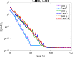
(a) F-norm of Riemannian gradient (iteration)

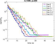
(b) F-norm of Riemannian gradient (time)

Figure 2: A comparison of gradient-descent algorithms with different metrics and retractions. Recall that $\mathrm{grad}f$ differs between the “E” and “C” methods, which explains why they do not have the same initial value.

First, we consider the optimization problem (1). We compare gradient-descent algorithms proposed in [12] with different metrics (Euclidean and canonical-like, denoted by “-E” and “-C”) and retractions (quasi-geodesics and Cayley transform, denoted by “Geo” and “Cay”). The canonical-like metric has two formulations, denoted by “-I” and “-II”, based on different choices of $X_{\perp}$. Hence, there are six methods involved. The problem generation and parameter settings are in parallel with ones in [12]. The numerical results are presented in Figure 2. Notice that the algorithms that use the Euclidean metric are considerably superior in the sense of the number of iterations. This can be partly explained by the structure of objective function in (1), which is indeed the Euclidean distance. Hence, in this problem the Euclidean metric may be more suitable than other metrics. However, due to their lower computational cost per iteration, algorithms with canonical-like-based Cayley retraction perform best with respect to time among all tested methods, and Cayley-based methods always outperform quasi-geodesics in each setting.

The second example is the symplectic eigenvalue problem. We compute the smallest symplectic eigenvalues and eigenvectors of symmetric positive-definite matrices in the sense of Williamson’s theorem; see [17]. According to the performance in Figure 2, we consider “Cay-E” and “Cay-C-I” as representative methods. The problem generation and default settings can be found in [17]. Note that the synthetic data matrix has five smallest symplectic eigenvalues $1,2,3,4,5$. In Table 1, we list the computed symplectic eigenvalues and $1$-norm errors. The results illustrate that our methods are comparable with the structure-preserving eigensolver “symplLanczos” based on a Lanczos procedure [2].

Table 1: Five smallest symplectic eigenvalues of a $1000\times 1000$ matrix computed by different methods

	symplLanczos	Cay-E	Cay-C-I
	0.999999999999997	1.000000000000000	0.999999999999992
	2.000000000000010	2.000000000000010	2.000000000000010
	3.000000000000014	2.999999999999995	3.000000000000008
	4.000000000000004	3.999999999999988	3.999999999999993
	5.000000000000016	4.999999999999996	4.999999999999996
Errors	4.75e-14	3.11e-14	3.70e-14

References

- [1] Absil, P.-A., Mahony, R., Sepulchre, R.: Optimization Algorithms on Matrix Manifolds. Princeton University Press (2008), https://press.princeton.edu/absil
- [2] Amodio, P.: On the computation of few eigenvalues of positive definite Hamiltonian matrices. Future Generation Computer Systems 22(4), 403–411 (2006). https://doi.org/10.1016/j.future.2004.11.027
- [3] Bartels, R.H., Stewart, G.W.: Solution of the matrix equation . Commun. ACM 15(9), 820–826 (1972). https://doi.org/10.1145/361573.361582
- [4] Benner, P., Fassbender, H.: An implicitly restarted symplectic Lanczos method for the Hamiltonian eigenvalue problem. Linear Algebra Appl. 263, 75–111 (1997). https://doi.org/10.1016/S0024-3795(96)00524-1
- [5] Benner, P., Fassbender, H.: The symplectic eigenvalue problem, the butterfly form, the SR algorithm, and the Lanczos method. Linear Algebra Appl. 275-276, 19–47 (1998). https://doi.org/10.1016/S0024-3795(97)10049-0
- [6] Benner, P., Kressner, D., Mehrmann, V.: Skew-Hamiltonian and Hamiltonian eigenvalue problems: Theory, algorithms and applications. In: Proceedings of the Conference on Applied Mathematics and Scientific Computing. pp. 3–39 (2005). https://doi.org/10.1007/1-4020-3197-1_1
- [7] Bhatia, R., Jain, T.: On symplectic eigenvalues of positive definite matrices. J. Math. Phys. 56(11), 112201 (2015). https://doi.org/10.1063/1.4935852
- [8] Birtea, P., Caşu, I., Comănescu, D.: Optimization on the real symplectic group. Monatsh. Math. 191, 465–485 (2020). https://doi.org/10.1007/s00605-020-01369-9
- [9] Buchfink, P., Bhatt, A., Haasdonk, B.: Symplectic model order reduction with non-orthonormal bases. Math. Comput. Appl. 24(2) (2019). https://doi.org/10.3390/mca24020043
- [10] Fiori, S.: Solving minimal-distance problems over the manifold of real-symplectic matrices. SIAM J. Matrix Anal. Appl. 32(3), 938–968 (2011). https://doi.org/10.1137/100817115
- [11] Fiori, S.: A Riemannian steepest descent approach over the inhomogeneous symplectic group: Application to the averaging of linear optical systems. Appl. Math. Comput. 283, 251–264 (2016). https://doi.org/10.1016/j.amc.2016.02.018
- [12] Gao, B., Son, N.T., Absil, P.-A., Stykel, T.: Riemannian optimization on the symplectic Stiefel manifold. arXiv preprint arXiv:2006.15226 (2020)
- [13] Golub, G.H., Van Loan, C.F.: Matrix Computations. Johns Hopkins University Press, 4th edn. (2013)
- [14] Jain, T., Mishra, H.K.: Derivatives of symplectic eigenvalues and a Lidskii type theorem. Canadian Journal of Mathematics p. 1–29 (2020). https://doi.org/10.4153/S0008414X2000084X
- [15] Machado, L.M., Leite, F.S.: Optimization on quadratic matrix Lie groups (2002), http://hdl.handle.net/10316/11446
- [16] Peng, L., Mohseni, K.: Symplectic model reduction of Hamiltonian systems. SIAM J. Sci. Comput. 38(1), A1–A27 (2016). https://doi.org/10.1137/140978922
- [17] Son, N.T., Absil, P.-A., Gao, B., Stykel, T.: Symplectic eigenvalue problem via trace minimization and Riemannian optimization. arXiv preprint arXiv:2101.02618 (2021)
- [18] Wang, J., Sun, H., Fiori, S.: A Riemannian-steepest-descent approach for optimization on the real symplectic group. Math. Meth. Appl. Sci. 41(11), 4273–4286 (2018). https://doi.org/10.1002/mma.4890
- [19] Williamson, J.: On the algebraic problem concerning the normal forms of linear dynamical systems. Amer. J. Math. 58(1), 141–163 (1936). https://doi.org/10.2307/2371062
- [20] Wu, R.B., Chakrabarti, R., Rabitz, H.: Critical landscape topology for optimization on the symplectic group. J. Optim. Theory Appl. 145(2), 387–406 (2010). https://doi.org/10.1007/s10957-009-9641-1
- [21] Wu, R., Chakrabarti, R., Rabitz, H.: Optimal control theory for continuous-variable quantum gates. Phys. Rev. A 77(5), 052303 (2008). https://doi.org/10.1103/PhysRevA.77.052303