Scalable Causal Domain Adaptation

Abstract

One of the most critical problems in transfer learning is the task of domain adaptation, where the goal is to apply an algorithm trained in one or more source domains to a different (but related) target domain. This paper deals with domain adaptation in the presence of covariate shift while invariance exist across domains. One of the main limitations of existing causal inference methods for solving this problem is scalability. To overcome this difficulty, we propose SCTL, an algorithm that avoids an exhaustive search and identifies invariant causal features across source and target domains based on Markov blanket discovery. SCTL  does not require having prior knowledge of the causal structure, the type of interventions, or the intervention targets. There is an intrinsic locality associated with SCTL that makes it practically scalable and robust because local causal discovery increases the power of computational independence tests and makes the task of domain adaptation computationally tractable. We show the scalability and robustness of SCTL for domain adaptation using synthetic and real data sets in low-dimensional and high-dimensional settings.

1 Introduction

Standard supervised learning usually assumes that both training and test data are drawn from the same distribution. However, this is a strong assumption and often violated in practice if (1) training examples have been obtained through a biased method (i.e., sample selection bias), or (2) there exist a significant physical or temporal difference between training and test data sources (i.e., non-stationary environments) [23]. Domain adaptation approaches aim to learn domain invariant features to mitigate the problem of data shift and enhance the quality of predictions [40, 49, 31].

Many domain adaptation techniques in the literature consider the covariate shift [7, 56, 50, 22, 19], where the marginal distribution of the features differs across the source and target domains, while the conditional distribution of the target given the features does not change. In causal inference, it has been noted that covariate shift corresponds to causal learning, i.e., predicting effects from causes [44]. Therefore, taking into account the causal structure of a system of interest and finding causally invariant features in both source and target domains enable us to safely transfer the predictions of the target variable based only on causally invariant features to the target domain [25, 42, 52, 53]. Following the same line of work, in this paper, we formalize and study the problem of domain adaptation as a feature selection problem where we aim to find an optimal subset that the conditional distribution of the target variable given this subset of predictors is invariant across domains under certain assumptions, as formally discussed in section 3. To illustrate the importance and effectiveness of this approach, consider the following example.

Example 1 (Domain Adaptation: Prediction of Diabetes at Early Stages).

According to Diabetes Australia, early diagnosis and initiation of appropriate treatment plays a pivotal role in: (1) helping patients to manage the disease early and (2) reducing the substantial economic impact of diabetes on the healthcare systems and national economies (700 million dollars each year [3]). To predict diabetes using machine learning techniques, we need its symptoms and clinical data. The common symptoms and possible causes of diabetes Type II are weakness, obesity, delayed healing, visual blurring, partial paresis, muscle stiffness, alopecia, among others [1]. Although we do not know what causes diabetes Type II [3], one may argue that the occurrence, rate, or frequency of Delayed Healing, Blurred Vision, Partial Paresis, and Weakness increases with age, and Delayed Healing and Partial Paresis may cause some complications that result in pancreas malfunction.

(a) Causal Graph for Diabetes

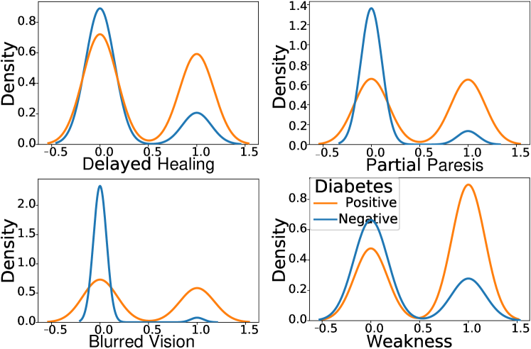
(b) Diabetes (Young Patients)

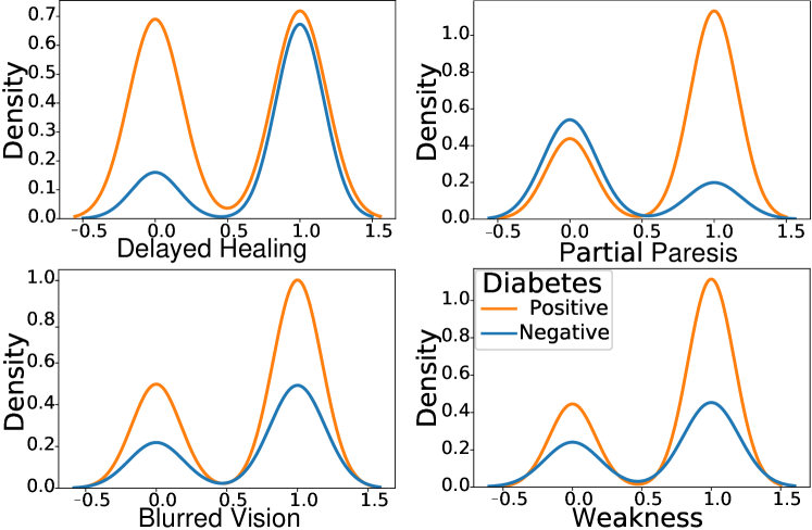
(c) Diabetes (Old Patients)

Figure 1: Prediction of Diabetes at an early stage: Here, age intervention leads to a shift of distributions between the source (Young Patients $<50$) and target (Old Patients $\geq 50$) domains (see also Example 1). In all cases, the orange curves indicate the distribution of tested positive patients, and the blue curves indicate the distribution of tested negative patients. A standard feature selection method that does snot consider the causal structure and would use all features to predict Diabetes would obtain biased predictions in the target domain (MSE = 0.29 and SSE = 65.322). Using only Delayed Healing and Partial Paresis instead yields less accurate predictions in the source domain, but much more accurate ones in the target domain (MSE = 0.221 and SSE = 49.8927).

The causal graph of this scenario can be represented as the directed acyclic graph (DAG) in Figure 1 (a). To provide an instance of a domain adaptation problem, we divided a diabetes dataset [15] into two subpopulations: (1) source domain with patients of the age less than 50 (dubbed young) and (2) target domain with patients of the age greater than or equal to 50 (old patients). As shown in Figure 1 (b) and (c), intervention in age leads to shifting distributions across domains. In our experiments, feature selection methods that do not consider the causal structure select highly relevant features to diabetes, i.e., all four variables Delayed Healing, Blurred Vision, Partial Paresis, and Weakness to achieve high prediction accuracy in the source domain. This per se causes worse predictions in the target domain (MSE = 0.29 and SSE = 65.322) than the case that we only consider causally invariant features, i.e., Delayed Healing and Partial Paresis for predictions in the target domain (MSE = 0.221 and SSE = 49.8927). The reason is that conditioning on the variables Blurred Vision and Weakness makes the paths between age and diabetes open, and hence the set of all features does not generalize to the target domain. However, conditioning only on Delayed Healing and Partial Paresis blocks the paths between age and diabetes. Hence, these causally invariant features enable us to predict diabetes with higher accuracy in the target domain, even in distribution shifts due to the age intervention.

An important limitation of existing causal inference methods [25, 42, 52, 53] is that they, currently, do not scale beyond dozens of variables due to either exponentially large number of conditional independence (CI) tests or difficulties in causal structure recovery [20]. To overcome the problem of scalability, we propose an algorithm based on Markov blanket discovery (see Appendix A for the definition) that in contrast to existing methods: (1) it takes advantage of local computation by finding only the Markov blanket of the target variable(s), and hence (2) reduces the search space for finding causally invariant features drastically because of the small size of Markov blankets ($\leq 10$) in (many) causal models in practice, e.g., see [46]. As a result, the CI tests becomes more reliable and robust when the number of variables increases, an essential characteristic in high dimensional and low sample size scenarios. Our main contributions are as follows:
$\bullet$ We propose a new algorithm, called Scalable Causal Transfer Learning (SCTL), to solve the problem of domain adaptation in the presence of covariate shift and scales to high-dimensional problems (section 3).
$\bullet$ For the first time we characterize Markov blankets in Acyclic Directed Mixed Graphs (ADMGs) i.e., causal graphs in the presence of unmeasured confounders, and we prove that the standard Markov blanket discovery algorithms such as Grow-Shrink (GSMB), IAMB and its variants are still correct under the faithfulness assumption where causal sufficiency is not assumed. We prove the correctness of SCTL based on these new theoretical results (section 3).
$\bullet$ We demonstrate on synthesized and real-world data that our proposed algorithm improves performance over several state-of-the-art algorithms in the presence of covariate shift (section 5). Code and data for reproducing our results is available at supplementary materials. https://github.com/softsys4ai/SCTL.

2 Related Work

Domain Adaptation. Here, we provide a brief overview of the main domain adaptation scenarios that can be found in the literature. There are three main domain adaptation problems: (1) Covariate shift, which is one of the most studied forms of data shift, occurs if the marginal distributions of context variables change across the source and target domains while the posterior (conditional) distributions are the same between source and target domains [47, 54, 16]. (2) Target shift occurs if the marginal distributions of the target variable change across the source and target domains while the posterior distributions remain the same [51, 62, 24]. (3) Concept shift occurs if marginal distributions between source and target domains remain unchanged while the posteriors change across the domains [28, 61, 14]. We only focus on the covariate shift in this paper. Since assuming invariance of conditionals makes sense if the conditionals represent causal mechanisms [42], we use the relaxed version of the usual covariate shift assumption and assume that it holds for a subset of predictor variables, as suggested and used in [42, 25].

Causal Inference in Domain Adaptation. Here, we briefly provide an overview of causal inference methods that address the problem of covariate shift: (1) Transportability [33, 4, 5, 9] expresses knowledge about differences and commonalities between the source and target domains in a formalism called selection diagram. Using this representation and the do-calculus [32], enable us to derive a procedure for deciding whether effects in the target domain can be inferred from experiments conducted in the source domain(s). (2) Invariant Causal Prediction (ICP) techniques [36, 37, 38] search for finding a subset of variables to estimate individual regressions for each domain in a way that produces regression residuals with equal distribution across all domains. Theoretical identifiability guarantees for the set of direct causal predictors for ICP techniques are limited to the linear Gaussian models. In other words, when the model is non-linear, non-Gaussian, or there are latent confounders, there is no guarantee that the obtained set is the set of direct causal predictors [36, 38]. (3) Graph surgery [52, 53] removes variables generated by unstable mechanisms from the joint factorization to yield a distribution invariant to the differences across domains. (4) Graph pruning methods [25, 42] formalized as a feature selection problem in which the goal is to find the optimal subset that the conditional distribution of the target variable given this subset of predictors is invariant across domains. Both transportability and graph surgery methods need to know the causal model of interest in advance. However, learning causal models from data is a challenging task, especially in the presence of unmeasured confounders [13]. On the other hand, graph pruning methods do not rely on prior knowledge of the causal graph, but they currently do not scale beyond dozens of variables [20].

3 Theory

In this section, first, we prove that the domain adaptation task under the Causal Domain Adaptation (CDA) assumptions can be done effectively via searching inside the set of Markov blanket of the target variable $T$ rather than a brute-force search over all variables as it has been done in Exhaustive Subset Search (ESS) in [25], the closest work to SCTL. In the next section, we present an efficient and scalable algorithm, called the SCTL, that searches over the Markov blanket of the target variable $T$ to find causally invariant features that provide an accurate prediction for the target variable $T$ given the distribution shift in terms of context variables. To apply SCTL in practice, we need an algorithm for Markov blanket discovery in the presence of unmeasured confounders. For this purpose, we prove that GSMB, IAMB, and its variants are still sound under the faithfulness assumption, even when the causal sufficiency assumption does not hold. The proof of theorems can be found in Appendix B.

3.1 Problem: Causal Domain Adaptation

Here we formally state the causal domain adaptation task that we address in this work:

Task 1 (Domain Adaptation Task).

We are given data for a source and a target domain such that the marginal distribution of the context variable $C$ changes across domains. Assume the source and target domains data are complete (i.e., no missing values), except for all values of a specific target variable $T$. The task is to predict these missing values of the target variable $T$ given the available source and target domains data.

For predicting $T$ from a subset of features $S\subseteq V\setminus\{C,T\}$, where $T$ is the target variable, $C=\{C_{s\in D_{s}},C_{t\in D_{t}}\}$ is the context variable with the values $C_{s\in D_{s}}$ in the source domain(s) and the values $C_{t\in D_{t}}$ in the target domain (note that we can extend our formalism to multiple context variables), and $S$ is a set that separates $T$ from $C$ in the causal model, we define the transfer bias as $\hat{T}^{t}_{S}-\hat{T}^{s}_{S}$, where $\hat{T}^{t}_{S}:=\mathbb{E}(T|S,C=C_{t\in D_{t}})$ and $\hat{T}^{s}_{S}:=\mathbb{E}(T|S,C=C_{s\in D_{s}})$. We define the incomplete information bias as $\hat{T}^{t}_{V\setminus\{C,T\}}-\hat{T}^{t}_{S}$. The total bias when using $\hat{T}^{s}_{S}$ to predict $T$ is the sum of the transfer bias and the incomplete information bias:

$$\underbrace{\hat{T}^{t}_{V\setminus\{C,T\}}-\hat{T}^{s}_{S}}_{\text{total bias}}=\underbrace{\hat{T}^{t}_{S}-\hat{T}^{s}_{S}}_{\text{transfer bias}}+\underbrace{\hat{T}^{t}_{V\setminus\{C,T\}}-\hat{T}^{t}_{S}.}_{\text{incomplete information bias}}$$

For more details, see [25]. Note that using invariant features only guarantees transfer bias to be zero, but the incomplete information bias can be quite large for the invariant feature set. There is a trade-off between the two terms in the total bias expression, which is hard to determine because the two terms are not identifiable using the source data alone.

3.2 Assumptions

We consider the same assumptions as discussed in [25], the closest work to ours.

Assumption 1 (Joint Causal Inference (JCI) assumptions).

We consider that causal graph $G=(V,E)$ is an ADMG with the variable set $V$. From now on, we will distinguish system variables $X_{j\in J}$ describing the system of interest, and context variables $C_{i\in I}$ describing the context in which the system has been observed:
(a) Context variables are never caused by system variables: $(\forall j\in J,i\in I:X_{j}\rightarrow C_{i}\notin E)$,
(b) System variables are not confounded by context variables: $(\forall j\in J,i\in I:X_{j}\leftrightarrow C_{i}\notin E)$, (c) All pairs of context variables are confounded: $(\forall i,k\in I:C_{i}\leftrightarrow C_{k}\in E\textrm{, and }\forall i,k\in I:C_{i}\rightarrow C_{k}\notin E)$.

The case (a) in the assumption is called exogeneity and captures what we mean by “context”. Cases (b), (c) are not as important as the exogeneity and can be relaxed, depending on the application [25].

Assumption 2 (Causal Domain Adaptation (CDA) assumptions).

We consider a causal graph $G$ that satisfies Assumption 1. We say $G$ satisfies CDA assumptions if

(a) The probability distribution of $V$ and the causal graph $G=(V,E)$ satisfy Markov condition and faithfulness assumption,
(b) For the target variable $T$ and a set $A$ that $T\perp\!\!\!\perp A|S$ (i.e., $T$ is independent of $A$ given $S$) in the source domain we have the same CI in the target domain, where $\{T\}\not\subseteq A\cup S$,
(c) No context variable $C$ is the parent of the target variable $T$, i.e., $C\rightarrow T\notin E_{G}$.

Assumption 2(b) states that the pooled source and target domains distributions are Markov and faithful to the local causal structure around the target variable of interest $T$. This assumption implies that the causal structure of the target variable $T$ is invariant when going from the source to the target domain. Note that Assumption 2(b) of the CDA assumption in [25] is different from ours: both the pooled source and pooled target domains distribution are Markov and faithful to $G$’s subgraph, which excludes the context variable $C$. This strong assumption forces them to do an exhaustive search. Assumption 2(c) is strong and restrictive, which might not hold in real data sets. However, since interventions are local in their nature, if the interventions are targeted precisely, then Assumption 2(c) is more likely to be satisfied.

3.3 Theoretical Results

The following theorem enables us to localize the task of finding invariant features under the CDA assumptions.

Theorem 1.

Assume that CDA assumptions hold for the context $C_{i\in I}$ and system variables $X_{j\in J}$ given data for single or multiple source domains. To find the best separating set(s) of features that $m$-separate(s) $C_{i\in I}$ from the target variable $T$ in the causal graph $G$, it is enough to restrict our search to the set of Markov blanket, $\textrm{{Mb}}(T)$, of the target variable $T$.

Theorem 1 enables us to develop a new efficient and scalable algorithm, called Scalable Causal Transfer Learning (SCTL), that exploits locality for learning invariant causal features to be used for domain adaptation. Since CDA assumptions do not require causal sufficiency assumption, we need sound and scalable algorithms for Markov blanket discovery in the presence of unmeasured confounders. For this purpose, we first need to provide a graphical characterization of Markov blankets in ADMGs.

Let $G=(V,E,P)$ be an ADMG model. Then, $V$ is a set of random variables, $(V,E)$ is an ADMG, and $P$ is a joint probability distribution over $V$. Let $T\in V$, then the Markov blanket $\textbf{Mb}(T)$ is the set of all variables that there is a collider path between them and $T$. We now show that the Markov blanket of the target variable $T$ in an ADMG probabilistically shields $T$ from the rest of the variables. Under the faithfulness assumption, the Markov blanket is the smallest set with this property. Formally we have:

Theorem 2.

Let $G=(V,E,P)$ be an ADMG model. Then, $T{\!\perp\!\!\!\perp}_{p}V\setminus\{T,\textbf{Mb}(T)\}|\textbf{Mb}(T)$.

Our following theorem safely enables us to use standard Markov blanket recovery algorithms for domain adaptation task without causal sufficiency assumption:

Theorem 3.

Given the Markov assumption and the faithfulness assumption, a causal system represented by an ADMG, and i.i.d. sampling, in the large sample limit, the Markov blanket recovery algorithms GSMB [26], IAMB [55], Fast-IAMB [60], Interleaved Incremental Association (IIAMB) [55], and IAMB-FDR [35] correctly identify all Markov blankets for each variable. (Note that Causal Sufficiency is not assumed.)

4 SCTL: Scalable Causal Transfer Learning

SCTL addresses the task of domain adaptation by finding a separating set $S\subset V$, where $V$ is the set of context variables $C_{i\in I}$ and system variables $X_{j\in J}$ such that for the target variable $T$ we have $C_{i}\perp\!\!\!\perp T|S$, for every $i\in I$ in the source domain. Since Assumption 2(b) implies that this conditional independence holds across domains, if such a separating set $S$ can be found, $S$ is considered as a set of causally invariant features for $T$ across environments. Our SCTL algorithm, described in Algorithm 1, consists of two main steps:
Step 1. We find the Markov blanket of the target variable $T$, i.e., $\textrm{{Mb}}(T)$ (line 3 in Algorithm 1). Using the property of Markov blankets, i.e., $T\perp\!\!\!\perp V\setminus\{T,\textrm{{Mb}}(T)\}|\textrm{{Mb}}(T)$, if there is no context variable in the Markov blanket of the target variable $T$, then $T{\perp\!\!\!\perp}C_{i\in I}|\textrm{{Mb}}(T)$. This means that the Markov blanket of $T$ provides a minimal feature set required for predicting the target variable $T$ with maximum predictivity [2].

Step 2. If there exists a context variable $C$ in $\textrm{{Mb}}(T)$, we consider all possible subsets of the Markov blanket of the target variable $T$, $\textrm{{Mb}}(T)$, to find those subsets $S_{i}$s that satisfy the separating condition $T\perp\!\!\!\perp C_{i\in I}|S_{i}$. For this purpose, the algorithm filters out those subsets for which the $p_{value}$ is below the significance level $\alpha$, i.e., $T$ is not conditionally independent of the context variables given those sets. At the end of line 14, we have a list $S$ that contains all possible separating sets. If $S$ is empty, we abstain from making predictions as the domain adaptation task is unsuccessful. This may happen if there exists a context variable $C$ in the adjacency of the target variable $T$, which means the data set does not satisfy the CDA assumptions because it violates the Assumption 1(a), (b), or Assumption 2(c). In this case, the algorithm throws a failure because there is no subset of features that is causally invariant across domains. Otherwise, we sort the list $S$ based on the obtained prediction errors in the source domain (line 18). Then, the algorithm returns those subsets $sub_{i}$ in $S$ with the lowest prediction error in the source domain as the best possible separating sets, because according to Theorem 1, these sets $m$-separates $T$ from the context variable(s) and minimize(s) the transfer bias. The computational complexity of SCTL is discussed in the supplementary material.

Input: A Dataset with variable set $V$ is the set of context variables $C_{i\in I}$ and system variables $X_{j\in J}$, target variable T, and significance level $\alpha$.

1

Output: A list of separating sets or null.

2

// Step 1: Find $\textrm{{Mb}}(T)$, Markov blanket of $T$.

3 Set $S$ as an empty list;

4

5Find $\textrm{{Mb}}(T)$;

6

7if $\textrm{{Mb}}(T)\cap C_{i},_{i\in I}=\emptyset$  then

8       return $S=\textrm{{Mb}}(T)$;

9      

10 else

       // Step 2: Find a subset of $\textrm{{Mb}}(T)$ that makes $T$ $m$-separated from the context variable(s).

11      

      Set Subs = Subset($\textrm{{Mb}}(T)$) ;

        /* All possible combinations of subsets for the obtained set $\textrm{{Mb}}(T)$ */

12       for each $sub_{i}\in$ Subs  do

13             $p_{val}$ = $p_{value}(C_{i\in I}\perp\!\!\!\perp T|sub_{i})$ ;

14            

15            if $p_{val}>\alpha$ then

                   // This means $T$ is conditionally independent of the context variables given the set $sub_{i}$.

16                   Add $sub_{i}$ to S;

17                  

18             end if

19            

20       end for

21      if S = $\emptyset$ then

22             return null;

23            

24       end if

      Sort $S$ ;

        /* Sort the list $S$ in descending order based on prediction errors in the source domain(s) */

25       return a list of elements of $S$ with the lowest prediction error in the source domain(s);

26 end if

Algorithm 1 SCTL: A Scalable Transfer Learning Algorithm for Causal Domain Adaptation

Remark 1.

Assume the causal graph in Figure 3 with the binary context variables $C_{1}$, $C_{2}$, and the target variable $T$. Also, assume that the domain adaptation task is to predict the missing values of $T$ in the target domains ($C_{1}=1$), based on the observed data from the source domain ($C_{1}=0$) and the target domain without knowledge of the causal graph. In this case, the true Markov blanket of the target variable $T$ is the set of $\textrm{{Mb}}(T)=\{X,Y,C_{1}\}$. However, since the value of the context variable $C_{1}$ is fixed in the source domain, Markov blanket discovery algorithms cannot discover the true Markov blanket in such cases. If we have access to the part of the data with no missing values for $T$ in the target domain, which is a realistic scenario in some situations, e.g., clinical data from a target hospital, the data from the source and the target domains can be used for learning the true $\textrm{{Mb}}(T)$. Otherwise, the problem is reduced to Markov blanket discovery in the presence of missing data. For this purpose, we can use the proposed method in [12].

Remark 2.

It has already been suggested in [37, Theorem 3.5] that the optimal set of causally invariant features is a subset of the Markov blanket of the target variable, called stable blanket. Here, we highlight the differences between [37] and SCTL:
(1) In [37], the underlying causal structure for the system variables is considered as a DAG, which means there is no latent confounder among system variables (causal sufficiency assumption). In contrast, in our work, this restrictive assumption is relaxed. Note that causal sufficiency assumption is a strong assumption and often violated in practice. Moreover, the paper provides no theoretical guarantee that the stable blanket is a subset of the Markov blanket of the target variable $T$, $\textrm{{Mb}}(T)$, in the presence of latent confounders. In fact, the invariance principle used in [36] shows that the stable set returned by the ICP techniques is a subset of ancestors of $T$. However, in our work, Theorem 1 relaxes the causal sufficiency assumption and states that searching in $\textrm{{Mb}}(T)$ is enough to find causally invariant features even in the presence of latent confounders.
(2) In [37], the joint probability distribution of variables is assumed to be continuous and experimental evaluations are restricted to the linear Gaussian models, while in our work, there is no restriction on the type of data and the probability distribution of variables. In fact, in section C, we do a comprehensive evaluation that is not restricted to the linear Gaussian models.

Figure 2: Ground truth synthetic graph: The grey node U represents the unknown confounder connecting the context variables filled in green $C_{1}$ & $C_{2}$. The node in orange, T, represent the target variable.

Figure 3: Ground truth synthetic graph: The grey node U represents the unknown confounder connecting the context variables filled in green $C_{1}$ & $C_{2}$. The nodes in orange, like E, T, represent possible target variables. The central structure represented by solid lines is common to all graphs. The dashed lines and nodes are used to introduce variability in the structure across domains.

5 Experimental Results

Experimental results, over various settings as discussed in Section C, have been shown in Figure 7,7,7,7,11,11, and 11, the remaining results are in Appendix E.

5.1 Synthetic Dataset

SCTL outperforms (in some cases a comparable performance) other approaches in all environment settings, considered on the synthetic dataset. In Figure 7-11, we report the most complicated scenarios involving severe domain shifts, extreme sample sizes, and multiple ground truth models; results for other scenarios can be found in the supplementary material. SCTL is, overall, as good as or even better than the state-of-the-art feature selection and domain adaptation algorithms listed in section C.

Key highlights. (1) Scalability: ESS, the closest work to SCTL, employs CI test based feature selection by conducting an exhaustive search over the entire feature set, which increases the time required for subset generation exponentially, so cannot scale on datasets beyond ten variables. We used ESS for computation on a 12 variable synthetic dataset for 72 hours, and it crashed without generating any results. SCTL drastically reduces the time required for subset search as it searches only those variables in the locality of the target variable. Note that the target could be a subset of variables rather than a single variable; parallel computation can speed up Markov blanket recovery because Markov blankets of different nodes can be learned independently [45]. This makes  SCTL scalable to high-dimensional data and has potential applications in big data (as we will show in a real dataset with 400k variables in Section 5.3).
(2) Robustness to Conditional Independence Tests: In cases where CI tests have to be estimated from data, mistakes occur in keeping or removing members from the estimated separating sets. Erroneous CI tests’ primary source are large condition sets in high-dimensional low sample size scenarios  [8]. In such cases, the resulting changes in the CI tests can lead to different separating sets. However, SCTL based on Markov blanket discovery only uses a small fraction of variables in the vicinity of the target, increasing the reliance on CI tests, making the algorithm robust in practice. Our experimentation confirms that for most environment settings, where we know the ground truth causal graph, SCTL can find the correct invariant features (e.g., see Table 4 and 5 in the appendix).
(3) Quantitative analysis of results on Gaussian settings: Although we report only the most interesting scenarios in Figures 7-11, we notice that for Gaussian settings (see Figure 11 (b)), the error rates of many of these feature selection algorithms are slightly lower than SCTL. Considering total bias, as discussed in section 3, these approaches enjoy higher predictivity due to lower incomplete information bias. For example, in Figure 11 (b), Adaboost has a slightly lower MSE than SCTL for the specified setting. We perform t-tests and F-tests to confirm our observation from the results for all such scenarios. In these tests, we found that the difference in error rates is almost insignificant (Figures 24 - 32).
(4) Increase in Error on small sample size: We do see a slight increase in the error on small sample size setting for SCTL (see Figure 11 (b)). Further investigation reveals that, since we do not utilize the underlying ground truth graph structure, the lack of data is straining the Markov blanket algorithms, causing them sometimes incorrectly to learn the Markov blanket of the target variable. For example, for the setting in Figure 11 (b) using Figure 11 (a) as the ground truth, we found that the Markov blanket of the target variable $T$ using IAMB is $\{P,X,C_{1},G\}$. In this case, the Markov blanket is wrong, but the separating set learned $\{P,X\}$ was satisfactory and causally invariant.

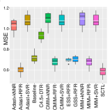
(a)

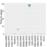
(b)

Figure 4: (a) prediction error, (b) runtime. Data shift: $C_{1}$ & $C_{2}$, target variable: $T$, sample size = 1000, data type: discrete, Ground truth: Figure 3 with solid lines.

(c)

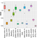
(d)

Figure 5: (a) the ground truth graph, (b) prediction error. Data shift: $C_{1}$, target variable: $T$, sample size = 1000, and data type: discrete.

(a)

(b)

Figure 6: (a) the ground truth graph, (b) prediction error. Data shift: $C_{1}$ & $C_{2}$, target variable: $T$, sample size = 1000, and data type: discrete.

(a)

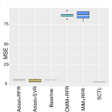
(b)

Figure 7: (a) the ground truth graph, (b) prediction error. Data shift: $C_{1}$, target variable: $M$, sample size = 1000, and data type: discrete.

(a)

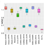
(b)

Figure 8: (a) the ground truth graph, (b) prediction error. Data shift: $C_{1}$ & $C_{2}$, target variable: $T$, sample size = 1000, and data type: discrete.

(c)

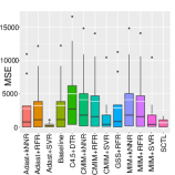
(d)

Figure 9: (a) the ground truth graph, (b) prediction error. No data shift, target variable: $T$, sample size = 1000, and data type: Gaussian.

(a)

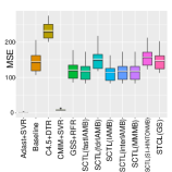
(b)

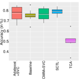
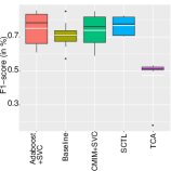
Figure 10: (a) the ground truth graph, (b) prediction error. Data shift: $C_{1}$ & $C_{2}$, target variable: $T$, sample size = 50, and data type: Gaussian.

Figure 11: Error rate comparison of feature selection approaches on the Diabetes dataset with Age Shift (discussed in Section C.1.2).

(5) Choice of Markov Blanket Algorithms: As shown in Figure 11 (b), the Markov blanket algorithm used holds key significance. Their practical uses may show results different from the theoretical perception. For example, GS does not consider the ordering and the strength of the association of the candidate variable and the target variable $T$. On the other hand, IAMB orders variables based on the strength of their association with the target variable $T$ first and then check their membership in the $\textrm{{Mb}}(T)$. Since choosing different p-values, the sample size of the data, and the maximum size of the conditioning sets have a big effect on the quality of learned $\textrm{{Mb}}(T)$, it is necessary to choose an appropriate Markov blanket approach depending on the given setting. For example, fdrIAMB [35] is particularly suitable when dealing with more nodes than samples in Gaussian models.

5.2 Real-world data: Diabetes Dataset

Although we do not have the ground truth causal graph for the real world diabetes data [15], we assume it follows Assumption 1 & 2. We consider Age as a context variable, because previous studies [18] have shown that older people are at higher risk of developing Type II diabetes. As this is a classification problem, the commonly used metrics Accuracy and F1-score were used to measure the algorithms’ performance. We compare SCTL against Adaboost and CMIM as they showed the best performance in the synthetic case. Similar to synthetic data, we ran  ESS on the computer for 72 hours, after which it was crashed. The results in Figure 11 show that although SCTL uses fewer features for prediction, it provides higher accuracy and F1-score in average compared with other approaches. We observe a more significant variability for Adaboost+SVC and CMIM+SVC accuracy and F1-score compared to SCTL as well as larger outliers. This can be considered an indication of the robustness of SCTL in real-world scenarios. On the other hand, although there is a greater variability for SCTL accuracy and F1-score compared to the baseline as well as larger outliers, SCTL enjoys higher accuracy and F1-score in general. These observations verify the importance of finding causally invariant features where data shift occurs. Notice that the total sample size for both training and testing scenarios had 200 entries for each. This signifies that even for a moderate number of samples, the Markov blankets can learn the vicinity of the target well enough for giving low error rates in the target domain. We also compared SCTL against Transfer Component Analysis (TCA), a state-of-the-art algorithm in unsupervised domain adaptation that identifies transfer components that remains invariant across domains. As shown in [30], the performance of TCA is sensitive to the choice of kernel choice and hyperparameters of the kernel function. We, therefore, performed hyperparameter tuning (details in Appendix) and reported the best result. We hypothesize that TCA cannot learn the transfer components correctly in this scenario and requires further investigations.

5.3 Real-world data: Cancer Dataset

To show the scalability of SCTL, we used the Colorectal Cancer Dataset. Similar to the diabetes case, we did not have the ground truth graph. For the same reasons, we compared SCTL against Adaboost and CMIM using Accuracy and F1-score. For this experiment, we considered Gender as the context variable. Firstly, this is a dataset with  400k variables, making it impossible to scale under any circumstances using [25].

Table 1: Results for the cancer dataset (100k ranked features)

Methodology	Accuracy	F1-Score
Baseline	91.25	90.94
SCTL (GS) (167 features)	88.12	87.88
SCTL (IAMB) (80 features)	96.25	96.22
CMIM + SVC	90.05	89.79
Adaboost	96.87	97.83

We conducted a sensitivity analysis to evaluate the robustness of algorithms in this high-dimensional and small sample size setting. For this purpose, we extracted 1000, 10k, and 100k features using an Extra-Trees classifier [34] to rank features based on their importance. In addition to the sensitivity analysis, by this intervention to the dataset, we made the setting in favor of feature selection algorithms that we compare by making the problem less dimensional and sorting the features based on their importance using the complete dataset (details in Appendix E). The results for each are shown in Tables 1, 2, and 3. We found SCTL to be either as good as or better than other approaches except in comparison to Adaboost, which enjoys slightly better performance than SCTL in (almost) all settings. We conjecture that this is due to a misalignment between theory and dynamics of the domain. It also is well-known that Adaboost is a successful classifier that takes advantage of boosting [59]. Although non-causal feature selection methods such as Adaboost are often used in practice, they cannot be interpreted causally even when they achieve excellent predictivity. Note that the size of the returned feature set for SCTL(IAMB) in Table 1 is considerably smaller than for SCTL(GS); the performance of SCTL(IAMB) is better than SCTL(GS). This indicates that IAMB is a better choice than GS in high-dimensional settings, as discussed in key highlight (5) for synthetic experiments.

Conclusion

In this paper, we proposed a new algorithm, called Scalable Causal Transfer Learning (SCTL), that identifies causal invariance in the presence of covariate shift and showed that it scales to high-dimensional and robust in low sample size settings in both synthetic and real-world scenarios. Weakening Assumption 2(b) and relaxing Assumption 2(c) are interesting directions for future work.

Appendix A Basic Definitions and Concepts

Assume that $G=(V,E)$ is a directed graph, where $V=\{v_{1},v_{2},v_{3}\cdots v_{n}\}$ is the set of nodes (variables), $n\geq 1$, and $E$ is the set of directed or bidirected edges. We say $v_{i}$ is a parent of $v_{j}$ and $v_{j}$ is a child of $v_{i}$ if $v_{i}\rightarrow v_{j}$ is an edge in $G$. We denote the set of parents and children of a variable $v$ by $\textrm{{pa}}(v)$ and $\textrm{{ch}}(v)$, respectively. Any bidirected edge $v_{i}\leftrightarrow v_{j}$ means that there exists a node $v_{k}\not\in V$ as a hidden confounder, such that $v_{i}\leftarrow v_{k}\to v_{j}$. If $G$ is acyclic, then $G$ is an Acyclic Directed Mixed Graph (ADMG). Formally, $\textrm{{ne}}(T)=\textrm{{pa}}(T)\cup\textrm{{ch}}(T)\cup\{v\in V|v\leftrightarrow T\textrm{ is a bidirected edge in }G\}$ refers to the neighbours of $T$. We define spouses of $v$ as $\textrm{{sp}}(v)=\{u\in V|\exists w\in V\textrm{ s.t. }u\to w\leftarrow v\textrm{ in }G\}$. We define Markov blanket of node $T$ as $\textrm{{Mb}}(T)=\textrm{{pa}}(T)\cup\textrm{{ch}}(T)\cup\textrm{{sp}}(T)$ when $G$ is a directed acyclic graph (DAG) and the set of children, parents, and spouses of $T$, and vertices connected with $T$ or children of $T$ by a bidirected path (i.e., only with edges $\leftrightarrow$) and their respective parents is the Markov blanket of $T$ when $G$ is an ADMG.

A path of length $n$ from $x$ to $y$ in an ADMG $G=(V,E)$ is a sequence $x=a_{0},\dots,a_{n}=y$ of distinct vertices such that $(a_{i},a_{i+1})\in E$, for all $i=1,\dots,n$. A vertex $\alpha$ is said to be an ancestor of a vertex $\beta$ if either there is a directed path $\alpha\to\dots\to\beta$ from $\alpha$ to $\beta$, or $\alpha=\beta$. We apply this definition to sets: $\textrm{{an}}(X)=\{\alpha|\alpha\textrm{ is an ancestor of }\beta\textrm{ for some }\beta\in X\}$.

Definition 1.

A nonendpoint vertex $\zeta$ on a path is a collider on the path if the edges preceding and succeeding $\zeta$ on the path have an arrowhead at $\zeta$, that is, $\to\zeta\leftarrow,or\leftrightarrow\zeta\leftrightarrow,or\leftrightarrow\zeta\leftarrow,or\to\zeta\leftrightarrow$. A nonendpoint vertex $\zeta$ on a path which is not a collider is a noncollider on the path. A path between vertices $\alpha$ and $\beta$ in an ADMG G is said to be m-connecting given a set Z (possibly empty), with $\alpha,\beta\notin Z$, if:

(i) every noncollider on the path is not in Z, and

(ii) every collider on the path is in $\textrm{{an}}_{G}(Z)$.

If there is no path m-connecting $\alpha$ and $\beta$ given Z, then $\alpha$ and $\beta$ are said to be $m$-separated given Z. Sets X and Y are m-separated given Z, if for every pair $\alpha,\beta$, with $\alpha\in X$ and $\beta\in Y$, $\alpha$ and $\beta$ are m-separated given $Z$ (X, Y, and Z are disjoint sets; X, Y are nonempty). This criterion is referred to as a global Markov property. We denote the independence model resulting from applying the m-separation criterion to G, by $\Im_{m}$(G). This is an extension of Pearl’s $d$-separation criterion to mixed graphs in that in a DAG D, a path is $d$-connecting if and only if it is m-connecting.

Definition 2.

Let $G_{A}$ denote the induced subgraph of $G$ on the vertex set $A$, formed by removing from $G$ all vertices that are not in $A$, and all edges that do not have both endpoints in $A$. Two vertices $x$ and $y$ in an ADMG $G$ are said to be collider connected if there is a path from $x$ to $y$ in $G$ on which every non-endpoint vertex is a collider; such a path is called a collider path. (Note that a single edge trivially forms a collider path, so if $x$ and $y$ are adjacent in an ADMG then they are collider connected.) The augmented graph derived from $G$, denoted $(G)^{a}$, is an undirected graph with the same vertex set as $G$ such that $c\--d\textrm{ in }(G)^{a}\Leftrightarrow c\textrm{ and }d\textrm{ are collider connected in }G.$

Definition 3.

Disjoint sets $X,Y\neq\emptyset,$ and $Z$ ($Z$ may be empty) are said to be $m^{\ast}$-separated if $X$ and $Y$ are separated by Z in $(G_{\textrm{{an}}(X\cup Y\cup Z)})^{a}$. Otherwise, $X$ and $Y$ are said to be $m^{\ast}$-connected given $Z$. The resulting independence model is denoted by $\Im_{m^{\ast}}(G)$.

Richardson in [41, Theorem 1] shows that for an ADMG $G$, $\Im_{m}(G)=\Im_{m^{\ast}}(G)$.

The Markov condition is said to hold for $G=(V,E)$ and a probability distribution $P(V)$ if $\langle G,P\rangle$ satisfies the following implication: $\forall X,Y\in V,\forall Z\subseteq V\setminus\{X,Y\}:(X{\!\perp\!\!\!\perp}_{m}Y|Z\Longrightarrow X{\!\perp\!\!\!\perp}_{p}Y|Z)$. The faithfulness condition states that the only conditional independencies to hold are those specified by the Markov condition, formally: $\forall X,Y\in V,\forall Z\subseteq V\setminus\{X,Y\}:(X{\not\!\perp\!\!\!\perp}_{m}Y|Z\Longrightarrow X{\not\!\perp\!\!\!\perp}_{p}Y|Z)$.

Appendix B Proofs of Theoretical Results

To prove Theorem 1, we need the following definitions and propositions.

Definition 4 (District and Induced Markov Blanket [41]).

Let $G$ be an acyclic directed mixed graph. We first specify a total ordering $(\prec)$ on the vertices of $G$, such that $x\prec y\Rightarrow y\not\in\textrm{{an}}(x)$; such an ordering is said to be consistent with $G$. Let $pre_{G,\prec}=\{v|v\prec x\textrm{ or }v=x\}$. The district of $x$ in $G$ is $x$ and the set of vertices connected to $x$ by a path on which every edge is of the form $\leftrightarrow$, denoted $dis_{G}(x)$. So, $dis_{G}(x)=\{v|v\leftrightarrow\cdots\leftrightarrow x\in G\textrm{ or }v=x\}$. A set $A$ is said to be ancestral if it is closed under the ancestor relation, i.e., if $\textrm{{an}}(A)=A$. If $A$ is an ancestral set in an ADMG $G$, and $x$ is a vertex in $A$ that has no children in $A$ then we define the Markov blanket of a vertex $x$ with respect to the induced subgraph on $A$, called induced Markov blanket, as the following: $imb_{A}(x)=\textrm{{pa}}_{G_{A}}(dist_{G_{A}}(x))\cup(dist_{G_{A}}(x)\setminus\{x\})$. It is not difficult to see that if $A=\textrm{{an}}_{G}(T)$, then $imb_{A}(T)\subseteq\textrm{{Mb}}(T)$ by the definition of $\textrm{{Mb}}(T)$ in an ADMG.

Proposition 1.

Given two nodes $X$ and $Y$ in an ADMG $G$ and a set $S$ of nodes not containing $X$ and $Y$, there exists some subset of $S$ which $m$-separates $X$ and $Y$ if only if the set $S^{\prime}=S\cap\textrm{{an}}(X\cup Y)$ $m$-separates $X$ and $Y$.

Proof.

($\Rightarrow$) Proof by contradiction. Let $S^{\prime}=S\cap\textrm{{an}}(X\cup Y)$ and ${\langle X,Y\not|S^{\prime}\rangle}$, i.e., $S^{\prime}$ does not $m$-separates $X$ and $Y$ in $G$. Since $S^{\prime}\subseteq\textrm{{an}}(X\cup Y)$, it is obvious that $\textrm{{an}}(X\cup Y\cup S^{\prime})=\textrm{{an}}(X\cup Y)$. So, $X$ and $Y$ are not separated by $S^{\prime}$ in $(G_{\textrm{{an}}(X\cup Y)})^{a}$, hence there is an undirected path $C$ between $X$ and $Y$ in $(G_{\textrm{{an}}(X\cup Y)})^{a}$ that bypasses $S^{\prime}$ i.e., the path $C$ is formed from nodes in $\textrm{{an}}(X\cup Y)$ that are outside of $S$. Since $\textrm{{an}}(X\cup Y)\subseteq\textrm{{an}}(X\cup Y\cup S^{\prime\prime}),\forall S^{\prime\prime}\subseteq S$, then $(G_{\textrm{{an}}(X\cup Y)})^{a}$ is a subgraph of $(G_{\textrm{{an}}(X\cup Y\cup S)})^{a}$. Then, the previously found path $C$ is also a path in $(G_{\textrm{{an}}(X\cup Y\cup S^{\prime\prime})})^{a}$ that bypasses $S^{\prime\prime}$, which means that $X$ and $Y$ are not separated by any $S^{\prime\prime}\subseteq S$ in $(G_{\textrm{{an}}(X\cup Y\cup S^{\prime\prime})})^{a}$, which is a contradiction.

($\Leftarrow$) It is obvious. ∎

Now, we prove Theorem 1.

Proof of Theorem 1.

Let $G$ be a causal graph with variable set $V$ consisting of system variables $X_{j\in J}$ and context variables $C_{i\in I}$. Assume that $C\in C_{i\in I}$, $T$ is the target variable and $\textrm{{Mb}}(T)$ is the Markov blanket of $T$. We have two cases:

• $C\not\in\textrm{{Mb}}(T)$: In this case, $C{\!\perp\!\!\!\perp}T|\textrm{{Mb}}(T)$ due to the definition of Markov blanket.

• $C\in\textrm{{Mb}}(T)$. In this case we show that considering the CDA assumptions, every path between $C$ and $T$ is blocked by $imb_{A}(T)$, where $A=\textrm{{an}}_{G}(T)$, or there is no subset of variables that $m$-separates $C$ from $T$. Proposition 1 implies that in order to find an $m$-separating set between $C$ and $T$ it is enough to restrict our search to the set $\textrm{{an}}_{G}(C\cup T)=\{C\}\cup\textrm{{an}}_{G}(T)$. Assume $A=\textrm{{an}}_{G}(T)$, we have the following subcases:

  • $C\in A$ and $C\not\in imb_{A}(T)$. Using the ordered local Markov property for $G$ and Theorem 2 in [41] implies that $C{\!\perp\!\!\!\perp}_{m}T|imb_{A}(T)$. Note that $imb_{A}(T)\subseteq\textrm{{Mb}}(T)$ by the definition of $\textrm{{Mb}}(T)$.

  • $C\not\in A$ and $C\not\in imb_{A}(T)$. Since $imb_{A}(T)\subseteq A$ and $A$ is an ancestral set, then $\textrm{{an}}_{G}(imb_{A}(T))=A$ and $\textrm{{an}}_{G}(C\cup T\cup imb_{A}(T))=\{C\}\cup\textrm{{an}}_{G}(T)$. So, if there is an undirected path between $T$ and $C$ in $(G_{\textrm{{an}}_{G}(C\cup T\cup imb_{A}(T))})^{a}$, Lemma 4 in [41] implies that this path intersects with the set $imb_{A}(T)$. In other words, $C{\!\perp\!\!\!\perp}_{m}T|imb_{A}(T)$.

  • $C\in imb_{A}(T)$. Using Definition 4 implies that $C\in A$. In this case, there is no subset of variables that $m$-separates $C$ from $T$. Proof by contradiction: Assume that there is a subset of variables $Z$ that $m$-separates $C$ from $T$ in $G$. Proposition 1 implies that $S=Z\cap\textrm{{an}}_{G}(T\cup C)=Z\cap(\{G\}\cup\textrm{{an}}_{G}(T))=Z\cap\textrm{{an}}_{G}(T)$ must $m$-separate $T$ from $C$ in $G$. Since $C\in imb_{A}(T)$ and $imb_{A}(T)\subseteq\textrm{{an}}_{G}(T)$, then it is not difficult to see that in $(G_{\textrm{{an}}(T\cup C\cup S)})^{a}$, $C$ is directly connected to the vertex $T$. This means that $S$ does not $m$-separate $T$ from $C$ in $G$, which is a contradiction. The following simple example illustrates such situations:

Note that in all cases, the Markov condition and faithful assumptions guarantee the correctness of independence relationships. As we have shown in all cases under the CDA assumptions, to find a separating set of features that $m$-separates $C$ from the target variable $T$ in the causal graph $G$, it is enough to restrict our search to the set of Markov blanket $\textrm{{Mb}}(T)$ of the target variable $T$. In the case that $C_{i,i\in I}$ has more than one element, a similar argument can be used to prove the theorem.

Using any subset $S$ for prediction that satisfies the $m$-separating set property, implies zero transfer bias. So, the best predictions are then obtained by selecting a separating subset that also minimizes the source domain’s risk (i.e., minimizes the incomplete information bias). ∎

Correctness of Algorithm 1.

The correctness of Algorithm 1 follows from Theorem 1. ∎

Proof of Theorem 2.

It is enough to show that for any $A\in V\setminus\{T,\textbf{Mb}(T)\}$, $T{\!\perp\!\!\!\perp}_{m}A|\textbf{Mb}(T)$. For this purpose, we prove that any path between $A$ and $T$ in $G$ is blocked by $\textbf{Mb}(T)$. In the following cases ($A-{\!\!\!*}B$, where means $A-B$ or $A\to B$ and $A{{*\!\!\!}-{\!\!\!*}}B$ means $A-B$, $A\to B$, or $A\leftarrow B$) we have:

1. The path $\rho$ between $A$ and $T$ is of the form $A{{*\!\!\!}-{\!\!\!*}}\cdots{{*\!\!\!}-{\!\!\!*}}B\to T$. Clearly, $B\in\textrm{{Mb}}(T)$ blocks the path $\rho$.

2. The path $\rho$ between $A$ and $T$ is of the form $A{{*\!\!\!}-{\!\!\!*}}\cdots{{*\!\!\!}-{\!\!\!*}}C\leftarrow B\leftarrow T$. Clearly, $B\in\textrm{{Mb}}(T)$ blocks the path $\rho$.

3. The path $\rho$ between $A$ and $T$ is of the form $A{{*\!\!\!}-{\!\!\!*}}\cdots{{*\!\!\!}-{\!\!\!*}}C\to B\leftarrow T$. $C\in\textrm{{Mb}}(T)$ blocks the path $\rho$.

4. The path $\rho$ between $A$ and $T$ is of the form $A{{*\!\!\!}-{\!\!\!*}}\cdots{{*\!\!\!}-{\!\!\!*}}C\to D\leftrightarrow\cdots\leftrightarrow B\leftarrow T$, where $\omega=C\to D\leftrightarrow\cdots\leftrightarrow B\leftarrow T$ is the largest collider path between $T$ and a node on the path $\rho$. Since all nodes of $\omega$ are in the Markov blanket of $T$, $\forall X\in\omega,X\neq A$. So, $C\in\textrm{{Mb}}(T)$ blocks the path $\rho$.

5. The path $\rho$ between $A$ and $T$ is of the form $A{{*\!\!\!}-{\!\!\!*}}\cdots{{*\!\!\!}-{\!\!\!*}}C\to D\leftrightarrow\cdots\leftrightarrow B\leftrightarrow T$, where $\omega=C\to D\leftrightarrow\cdots\leftrightarrow B\leftarrow T$ is the largest collider path between $T$ and a node on the path $\rho$. Since all nodes of $\omega$ are in the Markov blanket of $T$, $\forall X\in\omega,X\neq A$. So, $C\in\textrm{{Mb}}(T)$ blocks the path $\rho$.

From the global Markov property, it follows that every $m$-separation relation in $G$ implies conditional independence in every joint probability distribution $P$ that satisfies the global Markov property for $G$. Thus, we have $T{\!\perp\!\!\!\perp}_{p}V\setminus\{T,\textbf{Mb}(T)\}|\textbf{Mb}(T)$. ∎

Now, we are ready to prove Theorem 3.

Sketch of proof of Theorem 3.

If a variable belongs to $\textbf{Mb}(T)$, then it will be admitted in the first step (Growing phase) at some point, since it will be dependent on $T$ given the candidate set of $\textbf{Mb}(T)$. This holds because of the causal faithfulness and because the set $\textbf{Mb}(T)$ is the minimal set with that property. If a variable $X$ is not a member of $\textbf{Mb}(T)$, then conditioned on $\textbf{Mb}(T)\setminus\{X\}$, it will be independent of $T$ and thus will be removed from the candidate set of $\textbf{Mb}(T)$ in the second phase (Shrinking phase) because the causal Markov condition entails that independencies in the distribution are represented in the graph. Since the causal faithfulness condition entails dependencies in the distribution from the graph, we never remove any variable $X$ from the candidate set of $\textbf{Mb}(T)$ if $X\in\textbf{Mb}(T)$. Using this argument inductively, we will end up with the $\textbf{Mb}(T)$. ∎

In order to show the details of the proof of the Theorem 3, we prove only the correctness of the Grow-Shrink Markov blanket (GSMB) algorithm without causal sufficiency assumption in details as following (for the other algorithms listed in Theorem 3, a similar argument can be used):

Proof of Correctness of the GSMB Algorithm.

By “correctness” we mean that GSMB is able to produce the true Markov blanket of any variable in the ground truth ADMG under Markov condition and the faithfulness assumption if all conditional independence tests done during its course are assumed to be correct.

Input: a set $V$ of nodes, a target variable $T$, and a probability distribution $p$ faithful to an unknown ADMG $G$.

Output: The Markov blanket of $T$ i.e., $\textrm{{Mb}}(T)$.

1 Set $S=\emptyset$;

/* Grow Phase: */

2 while $\exists X\in V\setminus\{T\}\textrm{ such that }X{\not\!\perp\!\!\!\perp}_{p}T|S$ do

3       $S\leftarrow S\cup\{X\}$;

/* Shrink Phase: */

4 while $\exists X\in S\textrm{ such that }X{\!\perp\!\!\!\perp}_{p}T|S\setminus\{X\}$ do

5       $S\leftarrow S\setminus\{X\}$;

6return ($\textrm{{Mb}}(T)\leftarrow S$);

Algorithm 2 The GS Markov Blanket Algorithm [26].

We first prove that there does not exist any variable $X\in\textrm{{Mb}}(T)$ at the end of the growing phase that is not in $S$. The proof is by induction (a semi-induction approach on a finite subset of natural numbers) on the length of the collider path(s) between $X$ and $T$. We define the length of a collider path between $X$ and $T$ as the number of edges between them. Let $s$ be the length of a largest collider path between $X$ and $T$.

• (Base case) For the base of induction, consider the set of adjacent of $T$ i.e., $\textrm{{adj}}(T)=\{X\in V|X\to T,X\leftarrow T,\textrm{ or }X\leftrightarrow T\}$. In this case, $\nexists S\subseteq V\setminus\{T,X\}\textrm{ such that }X{\!\perp\!\!\!\perp}_{m}T|S$ in $G$. The faithfulness assumption implies that $\nexists S\subseteq V\setminus\{T,X\}\textrm{ such that }X{\!\perp\!\!\!\perp}_{p}T|S$. So, at the end of the growth phase, all the adjacent of $T$ are in the candidate set for the Markov blanket of $T$.

• (Induction hypothesis) For all $1\leq n<s$, if there is a collider path between $X$ and $T$ of length, $n$ then $X\in\textrm{{Mb}}(T)$ at the end of the growing phase.

• (Induction step) To prove the inductive step, we assume the induction hypothesis for $n=s-1$ and then use this assumption to prove that the statement holds for $s$. Assume that $\rho=(v_{0}=T){*\!\!\!\!}\to v_{1}\leftrightarrow\cdots\leftrightarrow v_{s-1}\leftarrow{\!\!\!\!*}v_{s}$ is a collider path of length $s$. From the induction hypothesis, we know that $v_{i}\in\textrm{{Mb}}(T),\forall 1\leq i<s$ at the end of the grow phase. Using Definition 1 implies that $\rho$ is $m$-connected to $T$. This means that at some point of the grow phase $v_{s}$ falls into the set $S$. The faithfulness assumption implies that $\exists S\subseteq V\setminus\{T,v_{s}\}\textrm{ such that }v_{s}{\not\!\perp\!\!\!\perp}_{p}T|S$. So, at the end of the grow phase, all of $X$’s that there is a collider path between $X$ and $T$ fall into the candidate set for the Markov blanket of $T$.

For the correctness of the shrinking phase, we have to prove two things: (1) we never remove any variable $X$ from $S$ if $X\in\textrm{{Mb}}(T)$, and (2) if $X\not\in\textrm{{Mb}}(T)$, $X$ is removed in the shrink phase.

Now, we prove case (1) by contradiction. Assume that $X\in\textrm{{Mb}}(T)$, $X\in S$ at the end of the grow phase, and we remove $X$ from $S$ in the shrink phase. This means $X\!\perp\!\!\!\perp_{p}T|S\setminus\{X\}$. Using the faithful assumption implies that $X\!\perp\!\!\!\perp_{m}T|S\setminus\{X\}$ i.e., $S\setminus\{X\}$ $m$-separates $X$ from $T$ in $G$, which is a contradiction because there is a collider path between $X$ and $T$ and $\textrm{{Mb}}(T)\setminus\{X\}\subseteq S$. In other word, the collider path between $X$ and $T$ is $m$-connected by $S\setminus\{X\}$.

To prove the case (2), assume that $X\not\in\textrm{{Mb}}(T)$, $\textbf{Y}=S\setminus\{\textrm{{Mb}}(T)\}$, and $X\in\textbf{Y}$. Due to the Markov blanket property, $\textrm{{Mb}}(T)$ $m$-separates Y from $T$ in $G$. Using the Markov condition implies that $\textbf{Y}\!\perp\!\!\!\perp_{p}T|\textrm{{Mb}}(T)$. Since the probability distribution $p$ satisfies the faithfulness assumption, it satisfies the weak union condition [43]. We recall the weak union property here: $A\!\perp\!\!\!\perp_{p}BD|C\Rightarrow(A\!\perp\!\!\!\perp_{p}B|DC\textrm{ and }A\!\perp\!\!\!\perp_{p}D|BC)$. Using the weak union property for $\textbf{Y}\!\perp\!\!\!\perp_{p}T|\textrm{{Mb}}(T)$ implies that $X\!\perp\!\!\!\perp_{p}T|(\textrm{{Mb}}(T)\cup(\textbf{Y}\setminus\{X\}))$, which is the same as $X\!\perp\!\!\!\perp_{p}T|(S\setminus\{X\})$. This means, $X\not\in\textrm{{Mb}}(T)$ will be removed at the end of the shrink phase. ∎

Appendix C Experimental Evaluation

We empirically validated the robustness and scalability of SCTL on both synthetic (10-20 variables) and real-world high-dimensional data (400k variables) by comparing with various feature selection approaches including Conditional Mutual Information Maximization (CMIM) [10], Mutual Information Maximization (MIM) [21], Adaboost (Adast) [11], Greedy Subset Search (GSS) [42], C4.5 using Decision Trees (C4.5 + DTR) [39] and Exhaustive Subset Search (ESS) [25].

C.1 Experimental Settings

In this section, we mention the different criteria used for data generation, parameter-tuning and validation. Based on changes in parameters and user dependent variables, we divide this section into three key parts. In each subsection we describe the combinations of hyperparameters used, why we used them and how they were implemented in practice.

C.1.1 Synthetic Data Generation

Let us consider an ADMG $G$ as shown in Figure 3. The basic synthetic dataset based on $G$ consists of 19 randomly generated variables, with 16 system variables, 2 context variables ($C_{1}$ & $C_{2}$) and 1 unknown confounder ($U$) (to be removed while using data). The data were generated in Gaussian as well as Discrete distributions. In Figure 3 the dashed lines and circles annotate the supplementary additions to the central structure which is represented by solid lines. We generate a dataset (see Appendix D for details) with desired number of samples and faithful w.r.t $G$. This data (not the graph structure) is used further for our experiments. We generated multiple datasets using different configurations to simulate the behaviour across different domain changes. These configurations were carefully generated to exploit characteristics of real-world scenarios:
(1) Changes to the sample size: We generated distributions with high disparity in the “amount” of data. The generated datasets contained 50, 1000 and 10000 cases. This would help us to see the difference in accuracy and robustness of the feature selection algorithms under extreme data-sensitive conditions (i.e., low sample size, moderate size, big data).
(2) Changes to the network size: We change the size of the graph, by increasing or dropping the number of nodes to monitor change in performance, to ensure scalability of the approach to changes in the number of environment variable. For this, we consider 3 different network sizes 20, 12 and 8 nodes, as shown in Figure 3 (further instances in Appendix). We also experimented by making changes to and on the number of context variables. This was done by using variables that are either partly, or completely unaffected by them (e.g., in Figure 3, we can use the whole or parts of graph with nodes $M$, $N$, $E$ as target).
(3) Changes to the complexity: The difference in complexity of the dataset can be further divided into structural change i.e., changing the edge connections or relations among the nodes (e.g., in Figure 3, we can add Z to induce affect of $C_{1}$ on the target $T$, or connect B and P, to affect the Markov blanket of $T$), and domain-distribution change i.e., changes between the source and target domain. Since we consider two context variables, domain-distribution change can be brought about by changes in either one or both. The changes to the domain can be classified further into three sub-settings: smooth (very little change to context variable), mild (small change in context variables) and severe (drastic change in context variables between source and target) by varying the mean and variance for Gaussian distributions and changing the probabilities associated with the variables in discrete distributions. To ensure consistency in our results, for each setting, we generate 8 test datasets, by making slight changes to any one of the system variables at random. The slight change is made so that the algorithms used for prediction do not report the same error each time, instead an error range serves a better depiction of practical robustness.

C.1.2 Real-world Dataset: Low-dimensional

We used the diabetes dataset [15] that reports common diabetic symptoms of 520 persons and contains 17 features, with 320 cases of diabetes Type II positive and 200 of diabetes negative patients. In the dataset, we consider two context variables, Age and Gender. We perform 3 sets of data shifts between training and testing domains using these context variables: (1) Gender Shift: We train on the Male and test on the Female. (2) Age Shift: We split the data using an arbitrary threshold (we choose 50 as threshold for our experimentation as it gives a fair distribution of samples between training and testing data), train on young (less than 50) and test on the old (greater than 50). (3) Double context shift: In this case, we train on young male patients and test on old female patients. We trained by sampling 100 samples from the source domain, keeping the samples in target domain constant to generates conditions for multiple source domains and single target domain. Such conditions help further test the robustness of the feature selection algorithm.

C.1.3 Real-world Dataset: High-dimensional

To assess  SCTL in a high-dimension, low-sample size real world setting, we experiment on the Colorectal Cancer Dataset [57]. It contains 334 samples assigned to three cancer risk groups (low, medium, and high) based on their personal adenoma or cancer history. The entire dataset contains $\sim$ 400k features. We perform 2 sets of possible data shifts between training and testing domains using these context variables: (1) Gender Shift: We train on the Male and test on the Female. (2) Age Shift: We split the data using an arbitrary threshold, in our experiments, train on young (less than 50) and test on the older (greater than 50).

C.2 Evaluation Metrics

We tested SCTL and other algorithms using different regression techniques such as RFR, SVR, and kNNR, in order to mitigate doubts about approach specific biases. We found, for SCTL, the same error more or less in (almost) all cases, but we chose Random Forest Regressor as it not only performed well, but also, gave consistent results. Here, the Baseline indicates using all available features and feeding it to the Random Forest Regressor. We reported accuracy with Mean-Square-Error (MSE) and time taken in second.

Appendix D Details of Experimental Evaluation

The data generation processes, conditional independence tests and Markov blanket Algorithms were implemented in R by extending the bnlearn [45] and pclag [17] packages. We used Python 3.6 with scikit-learn [34] library for implementing the above-mentioned feature selection and machine learning algorithms to compare our approach against. The library is also used for prediction over subset of features selected by SCTL using RandomForestRegressor function. The generated predictions from each of the algorithms are compared to the actual results for finding the error and all experiments have been reported using various comparison metrics.

Synthetic Data Generation

For Gaussian setting, a model graph as shown in Figure 3 was generated using model2network function from the graphviz package. The obtained DAG from Figure 3 is passed to the custom.fit function from bnlearn which defines the mean, variance and relationship (edges values) between the nodes. This process ensures that the generated dataset will be faithful w.r.t $G$. Once the graph is set and all variables have been properly defined, we use the rbn function from bnlearn to generate the required number of samples.

For the Discrete setting, the same process is followed, but instead of mean, variance and edge values, we use a matrix of random probabilities. For each node, the size of the matrix would be the number of discrete values for the node, plus the number of discrete values for each of its connecting nodes multiplied by the number of modes connected to it.

Implementation Parameters

SCTL requires the use of Markov-blanket and neighborhood for feature selection. We use multiple Markov blanket discovery-algorithms to evaluate the effect the algorithm-choice can have on final prediction. For this purpose, we select, GS, IAMB, interIAMB, fastIAMB, fdrIAMB, MMMB, SI.HINTON.MB. These algorithms were implemented in R using the bnlearn package. The variable subs mentioned on line 12 of Algorithm 1 contains all possible combination of subsets from the feature set $S_{2}$. To find all possible subsets of a given feature set we use Python 3.5, one or more of these subsets will act as the separating set. To find the separating set, we sort the subsets based on $p_{value}$ of conditional independence tests and choosing the subset/s with the highest score. We use a significance level $\alpha$ of 0.05 as threshold for the conditional independence tests. The tests for different configurations are based on the type of data being used. For Gaussian data, we used gaussCItest from the pclag package, which uses Fisher’s z-transformation of the partial correlation, for testing correlation for sets of normally distributed random variables. For discrete data, we use the mutual information (mi) test (an information-theoretic distance measure, which is somewhat proportional to the log-likelihood ratio) from the bnlearn package.

Change to the complexity

As an example, for a central structure consist of 8 nodes as shown in Figure 3 having 10000 samples with severe changes in context, we train by generating one dataset on the base setting. Then make severe changes to the domain-distribution (i.e., by drastically changing the values of the context variables) and then generate a new dataset which is used for testing.

Evaluation Metrics

We used the RandomForestRegressor function from scikit-learn package, using the out-of-bag (OOB) scoring approach on the default parameters, for this process.

Appendix E More Experimental Results

In this section, we include the remaining results that we got during experimentation, along with a subsequent ground truth graph for representing the various settings we experiment on synthetic data. In the later part of this section we also include t-test tables as mentioned in Section 5. More experimental results regarding synthetic data can be found at the end of this appendix.

E.1 Real-world Dataset: Low-dimensional

We used the diabetes dataset [15] that contains reports of common diabetic symptoms of 520 persons. This includes data about symptoms that may cause or are potentially caused by diabetes. The dataset has been created from a direct questionnaire to people who have either recently been diagnosed as diabetic, or who are still non-diabetic but having show few or more symptoms of diabetes. The diabetes dataset contains a total of 17 features, with 320 cases of diabetes Type II positive and 200 of diabetes negative patients. The data has been collected from the patients of the Sylhet Diabetes Hospital, Sylhet, Bangladesh. In the dataset, we consider two context variables, Age, and Gender. We perform 3 sets of data shifts between training and testing domains using these context variables: (1) Gender Shift: We train on the Male and test on the Female. (2) Age Shift: We split the data using an arbitrary threshold (we choose 50 as threshold for our experimentation as it gives a fair distribution of samples between training and testing data), train on young (less than 50) and test on the older (greater than 50). (3) Double context shift: We do a dataset shift for both context variables, in our case, we train on young male patients and test on old female patients. In practice, while experimenting on a context shift setting we train by sampling 100 samples from the source domain, keeping the samples in the target domain constant. This allows us to generate conditions similar to having multiple source domains and single target domain. Such conditions will help further test the robustness of the feature selection algorithm.

E.2 Real-world Dataset: High-dimensional

To assess  SCTL  in a high-dimension, low-sample size real world setting, we experiment on the Colorectal Cancer Dataset [57]. Chronological age is a prominent risk factor for many types of cancers, including Colorectal Cancer, on which this dataset is based. The dataset is basically a genome-wide DNA methylation study on samples of normal colon mucosa, it contains 334 samples assigned to three cancer risk groups (low, medium, and high) based on their personal adenoma or cancer history. Our target variable for classification was the ‘Diagnosis’ feature, a binary variable which indicates whether or not the patient was diagnosed with cancer, the entire dataset contains ~400k features. We again perform 2 sets of data shifts between training and testing domains using these context variables: (1) Gender Shift: We train on the Male and test on the Female. (2) Age Shift: We split the data using an arbitrary threshold (we choose 50 as threshold for our experimentation as it gives a fair distribution of samples between training and testing data), train on young (less than 50) and test on the older (greater than 50).

Table 2: Cancer dataset (1000 ranked features) result

Methodology	Accuracy	F1-Score
Baseline	91.87	91.70
SCTL (GS) (167 features)	87.50	87.18
SCTL (IAMB) (13 features)	96.82	97.22
CMIM + SVC	87.5	87.06
Adaboost	96.87	97.83

Table 3: Cancer dataset (10k ranked features) result

Methodology	Accuracy	F1-Score
Baseline	91.25	90.94
SCTL (GS) (167 features)	88.125	87.88
SCTL (IAMB) (79 features)	97.5	97.65
CMIM + SVC	90.15	89.79
Adaboost	96.87	97.83

E.3 SCTL vs Unsupervised Domain Adaptation TCA

Transfer Component Analysis (TCA) is an unsupervised technique for domain adaptation proposed by Pan et al. [30] that discovers common latent features, called transfer components, that have the same marginal distribution across the source and target domains while maintaining the essential structure of the source domain data [58]. TCA learns these transfer components across domains in a reproducing kernel Hilbert space [48] using maximum mean miscrepancy [6]. Once the transfer components are found, a traditional machine learning technique is used to train the final target classifier. In short, TCA is a two-step domain adaptation technique where the first step reduces the marginal distributions between the source and target domains and the second step trains a classifier with the adapted domain data. Here, we compare SCTL against TCA, which is a state-of-the-art algorithm in unsupervised domain adaptation, and report the results. Note that, in TCA the focus is to identify substructures (i.e., transfer components) that remains invariant across domains, which is different from the problem of identifying invariant features used for training a predictive model, in which we do not need to have prior knowledge about the causal structure of the model that we are interested in. For implementation of the TCA we used, the rbf kernel, and the logistic classifier to predict on the extracted components. We also tune the hyperparameters of the algorithm by using Support Vector Classifier and increasing the number of components from 1 to 5, which lead to further decrease in the accuracy of the model. We hypothesize that TCA cannot learn the transfer components correctly in this setting. Further investigation by comparing with semi-supervised versions [30] as well as strategies that also incorporate sample reweighing are left for future work.

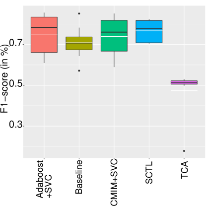
Figure 12: Error rate comparison of multiple feature selection approaches (supervised and unsupervised) on a simulation of the Diabetes dataset with Age Shift (discussed in Section C.1.2).

Table 4: Markov blanket and separating feature sets extracted by various algorithms on the target variable $T$ for Figure 32(a).

Methodology	Markov blanket	Separating set
GS	["K", "L", "N" , "Y"]	["K", "L","N", "Y" ]
IAMB	["K", "L", "N"]	["K", "L","N" ]
interIAMB	["K", "L", "N"]	["K", "L","N" ]
fastIAMB	["K", "L", "N", "Y"]	["K", "L","N","Y" ]
MMMB	["K", "L", "N"]	["K", "L","N" ]
fdrIAMB	["K", "L", "N"]	["K", "L","N" ]

Table 5: Markov blanket and separating feature sets extracted by various algorithms on the target variable $T$ for Figure 19(a).

Methodology	Markov blanket	Separating set
GS	["C1", "P", "X" , "Y" ]	["P", "X" ]
IAMB	["C1", "P" , "X" ,"Y"]	["P", "X" ]
interIAMB	["C1", "P", "X" , "Y" ]	["P", "X" ]
fastIAMB	["C1", "P", "X" , "Y" ]	["P", "X" ]
MMMB	["C1", "P", "X" , "Y" ]	["P", "X" ]
fdrIAMB	["C1", "P", "X" , "Y" ]	["P", "X" ]
ESS	NA	["Q", "X", "Y"]

Computational complexity of SCTL.

Assume that the “learning Markov blankets” phase (Step 1) uses the grow-shrink (GS) algorithm [27], and $n=|V|$, $m=|E|$, where $G=(V,E)$ is the unknown true causal structure. Since the Markov blanket algorithm involves $O(n)$ conditional independence (CI) tests, if the cardinality of the Markov blanket of the target variable is $k$ (in many real world cases $k<<n$, see for example real world datasets and their properties in [46]) then the total number of needed Cl tests for finding the best separating set is O$(n+2^{k})$, see [26] for more details. On the other hand, the brute force algorithm used in (Magliacane et al., 2018) needs O$(2^{n})$ tests in the worst case scenario, which is infeasible in practice as we have shown in our experiments. The same argument is valid when we have multiple target variables, say $c$, where $c<<n$.

(a)

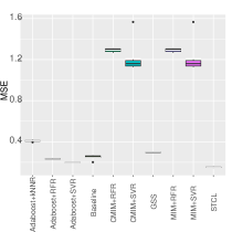
(b)

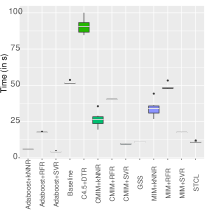
(c)

Figure 13: Results on (b), (c) are generated over the ground truth graph (a) for the target variable $T$. Data shift between source and target occurs by change in the probability distribution of the context variable $C_{1}$, where sample size = 10000 for a Gaussian distribution.

(a)

(b)

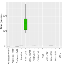
(c)

Figure 14: Results on (b), (c), (d) are generated over the ground truth graph (a) for the target variable $T$. Data shift between source and target occurs by change in the probability distribution of the context variable $C_{1}$, where sample size = 1000 for a Gaussian distribution.

(a)

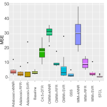
(b)

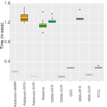
(c)

Figure 15: Results on (b), (c), (d) are generated over the ground truth graph (a) for the target variable $T$. Data shift between source and target occurs by change in the probability distribution of the context variable $C_{1}$, where sample size = 50 for a Gaussian distribution.

(a)

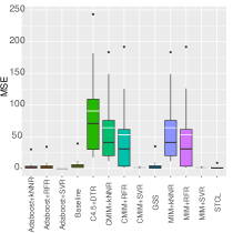
(b)

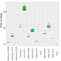
(c)

Figure 16: Results on (b), (c), (d) are generated over the ground truth graph (a) for the target variable $T$. Data shift between source and target occurs by change in the probability distribution of the context variable $C_{1}$& $C_{2}$, where sample size = 10000 for a Gaussian distribution.

(a)

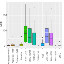
(b)

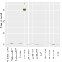
(c)

Figure 17: Results on (b), (c), (d) are generated over the ground truth graph (a) for the target variable $T$. Data shift between source and target occurs by change in the probability distribution of the context variable $C_{1}$ & $C_{2}$, where sample size = 1000 for a Gaussian distribution.

(a)

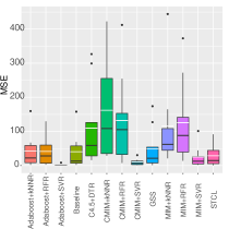
(b)

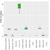
(c)

Figure 18: Results on (b), (c), (d) are generated over the ground truth graph (a) for the target variable $T$. Data shift between source and target occurs by change in the distribution of the context variable $C_{1}$ & $C_{2}$, where sample size = 50 for a Gaussian distribution.

(a)

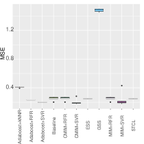
(b)

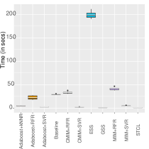
(c)

Figure 19: Results on (b), (c), (d) are generated over the ground truth graph (a) for the target variable $T$. Data shift between source and target occurs by change in the distribution of the context variable $C_{1}$, where sample size = 10000 for a Gaussian distribution.

(a)

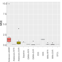
(b)

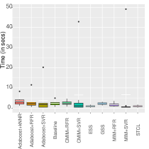
(c)

Figure 20: Results on (b), (c), (d) are generated over the ground truth graph (a) for the target variable $T$. Data shift between source and target occurs by change in the distribution of the context variable $C_{1}$, where sample size = 1000 for a Gaussian distribution.

(a)

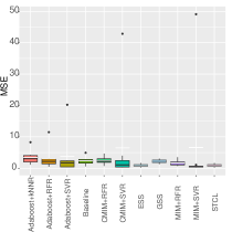
(b)

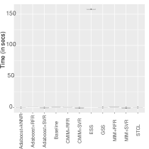
(c)

Figure 21: Results on (b), (c), (d) are generated over the ground truth graph (a) for the target variable $T$. Data shift between source and target occurs by change in the distribution of the context variable $C_{1}$, where sample size = 50 for a Gaussian distribution.

(a)

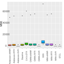
(b)

(c)

Figure 22: Results on (b), (c), (d) are generated over the ground truth graph (a) for the target variable $T$. Data shift between source and target occurs by change in the distribution of the context variable $C_{1}$ , where sample size = 1000 for a Gaussian distribution.

(a)

(b)

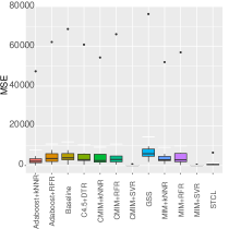
(c)

Figure 23: Results on (b), (c), (d) are generated over the ground truth graph (a) for the target variable $T$. Data shift between source and target occurs by change in the distribution of the context variable $C_{1}$ , where sample size = 50 for a Gaussian distribution.

(d)

Methodology	p-value
Baseline	0.1694
GSS	0.19617
CMIM+SVR	0.3187
CMIM+kNNR	0.1258
CMIM+RFR	0.1376
MIM+SVR	0.318705
MIM+kNNR	0.1258
MIM+RFR	0.13759
Adaboost+SVR	0.279
Adaboost+kNNR	0.20346
Adaboost+RFR	0.169
C4.5+ DTR	0.0889

(b)

Figure 24: Results in the table are p-values generated by performing a T-test on SSE over the ground truth graph (a) for the target variable T. Data shift between source and target occurs by change in the distribution of the context variable $C_{1}$, over a Gaussian distribution with sample size = 1000. The bold results indicate that the average performance of SCTL is not significantly different from the average performance of other approaches for the p-value 0.05.

(a)

Methodology	p-value
Baseline	0.1535
GSS	0.1681
CMIM+SVR	0.2712
CMIM+kNNR	0.1224
CMIM+RFR	0.1885
MIM+SVR	0.65673
MIM+kNNR	0.04307
MIM+RFR	0.16345
Adaboost+SVR	0.2660
Adaboost+kNNR	0.0526
Adaboost+RFR	0.1185
C4.5+ DTR	0.0295
ESS	0.0222

(b)

Figure 25: Results in the table are p-values generated by performing a T-test on MSE over the ground truth graph (a) for the target variable T. Data shift between source and target occurs by change in the distribution of the context variable $C_{1}$ & $C_{2}$ , over a Gaussian distribution with sample size = 1000. The bold results indicate that the average performance of SCTL  is not significantly different from the average performance of other approaches for the p-value 0.05.

(a)

Methodology	p-value
Baseline	0.01747
GSS	6.14934e-08
CMIM+SVR	2.9747e-08
CMIM+kNNR	0.00445
CMIM+RFR	1.7186e-17
MIM+SVR	5.415e-07
MIM+kNNR	0.0057
MIM+RFR	8.48536e-17
Adaboost+SVR	0.0001
Adaboost+kNNR	1.0681e-07
Adaboost+RFR	0.16304
C4.5+ DTR	4.2182e-08

(b)

Figure 26: Results in the table are p-values generated by performing a T-test on MSE over the ground truth graph (a) for the target variable T. Data shift between source and target occurs by change in the distribution of the context variable $C_{1}$ , over a Gaussian distribution with sample size = 1000. The bold results indicate that the average performance of SCTL  is significantly different from the average performance of other approaches for the p-value 0.05.

(a)

Methodology	p-value
Baseline	2.5901e-09
GSS	9.1341e-06
CMIM+SVR	0.7350
CMIM+kNNR	0.1154
CMIM+RFR	0.0265
MIM+SVR	0.94294
MIM+kNNR	0.1687
MIM+RFR	0.0190
Adaboost+SVR	0.87851
Adaboost+kNNR	9.9208e-09
Adaboost+RFR	0.1205
C4.5+ DTR	2.6341e-05
ESS	0.6341

(b)

Figure 27: Results in the table are p-values generated by performing a T-test on MSE over the ground truth graph (a) for the target variable T. Data shift between source and target occurs by change in the distribution of the context variable $C_{1}$, over Gaussian data with sample size = 1000. The bold results indicate that the average performance of SCTL is significantly better than the average performance of other approaches for the p-value 0.05.

(a)

Methodology	p-value
Baseline	0.0225
GSS	1.2961e-05
CMIM+SVR	1.212e-10
CMIM+kNNR	1.6860e-14
CMIM+RFR	0.0001
MIM+SVR	1.212e-10
MIM+kNNR	3.344e-14
MIM+RFR	0.0001
Adaboost+SVR	1.212e-10
Adaboost+kNNR	5.148e-13
Adaboost+RFR	0.1290
C4.5+ DTR	2.562e-10

(b)

Figure 28: Results in the table are p-values generated by performing a T-test on MSE over the ground truth graph (a) for the target variable T. Data shift between source and target occurs by change in the distribution of the context variables $C_{1}$& $C_{2}$, over Discrete data with sample size = 1000. The bold results indicate that the average performance of SCTL  is significantly better than the average performance of other approaches for the p-value 0.05.

(a)

Methodology	p-value
Baseline	0.00013
GSS	0.0001
CMIM+SVR	4.785e-10
CMIM+kNNR	5.4748e-10
CMIM+RFR	0.0059
MIM+SVR	4.7853e-10
MIM+kNNR	4.7034e-10
MIM+RFR	0.0056
Adaboost+SVR	4.785e-10
Adaboost+kNNR	7.088e-10
Adaboost+RFR	0.5531
C4.5+ DTR	3.136e-09
ESS	0.0006

(b)

Figure 29: Results in the table are p-values generated by performing a T-test on MSE over the ground truth graph (a) for the target variable T. Data shift between source and target occurs by change in the distribution of the context variables $C_{1}$& $C_{2}$, over Discrete data. The bold results indicate that the average performance of SCTL  is significantly better than the average performance of other approaches for the p-value 0.05.

(a)

Methodology	p-value
Baseline	0.0001
GSS	1.585e-06
CMIM+SVR	7.227e-15
CMIM+kNNR	4.352e-09
CMIM+RFR	5.212e-06
MIM+SVR	7.227e-15
MIM+kNNR	7.327e-09
MIM+RFR	0.0001
Adaboost+SVR	7.229e-15
Adaboost+kNNR	3.760e-08
Adaboost+RFR	0.054
C4.5+ DTR	8.380e-10

(b)

Figure 30: Results in the table are p-values generated by performing a T-test on MSE over the ground truth graph (a) for the target variable T. Data shift between source and target occurs by change in the distribution of the context variable $C_{1}$, over Discrete data. The bold results indicate that the average performance of SCTL  is significantly better than the average performance of other approaches for the p-value 0.05.

(a)

Methodology	p-value
Baseline	0.1651
GSS	0.1687
CMIM+SVR	3.5196e-07
CMIM+kNNR	0.0277
CMIM+RFR	0.066
MIM+SVR	3.519e-07
MIM+kNNR	0.0277
MIM+RFR	0.0664
Adaboost+SVR	0.3315
Adaboost+kNNR	0.1858
Adaboost+RFR	0.1865
C4.5+ DTR	0.0228

(b)

Figure 31: Results in the table are p-values generated by performing a T-test on MSE over the ground truth graph (a) for the target variable T. Data shift between source and target occurs by change in the distribution of the context variable $C_{1}$& $C_{2}$, over Discrete data with sample size = 10000. The bold results indicate that the average performance of SCTL  is comparable to the average performance of other approaches for the p-value 0.05.

(a)

Methodology	p-value
Baseline	6.7513e-12
GSS	0.0009
CMIM+SVR	0.0056
CMIM+kNNR	1.03614e-06
CMIM+RFR	1.2254e-11
MIM+SVR	1.0319e-05
MIM+kNNR	1.1642e-07
MIM+RFR	4.537e-10
Adaboost+SVR	0.0305
Adaboost+kNNR	0.0138
Adaboost+RFR	3.993e-10
C4.5+ DTR	2.0194e-07

(b)

Figure 32: Results in the table are p-values generated by performing a T-test on MSE over the ground truth graph (a) for the target variable M. Data shift between source and target occurs by change in the distribution of the context variable $C_{1}$, over Discrete data with sample size = 1000. The bold results indicate that the average performance of SCTL  is significantly better than the average performance of other approaches for the p-value 0.05.

References

- [1] American Diabetes Association (ADA). Statistics about diabetes. https://www.diabetes.org/, 2020.
- [2] Constantin F. Aliferis, Alexander Statnikov, Ioannis Tsamardinos, Subramani Mani, and Xenofon D. Koutsoukos. Local causal and markov blanket induction for causal discovery and feature selection for classification part i: Algorithms and empirical evaluation. JMLR, pages 171–234, 2010.
- [3] Diabetes Australia. Diabetes in Australia. https://www.diabetesaustralia.com.au, 2020.
- [4] Elias Bareinboim and Judea Pearl. Transportability of causal effects: Completeness results. In Proceedings of the 26th AAAI Conference on Artificial Intelligence, pages 698–704, Toronto, Ontario, Canada, Jul 2012. AAAI Press.
- [5] Elias Bareinboim and Judea Pearl. Transportability from multiple environments with limited experiments: Completeness results. In Z. Ghahramani, M. Welling, C. Cortes, N. D. Lawrence, and K. Q. Weinberger, editors, Advances in Neural Information Processing Systems 27, pages 280–288. Curran Associates, Inc., 2014.
- [6] Karsten M Borgwardt, Arthur Gretton, Malte Rasch, Hans-Peter Kriegel, Bernhard Schölkopf, and Alex Smola. Integrating structured biological data by kernel maximum mean discrepancy. Bioinformatics, 22(14):49–57, 2006.
- [7] Xiangli Chen, Mathew Monfort, Anqi Liu, and Brian D. Ziebart. Robust covariate shift regression. volume 51 of Proceedings of Machine Learning Research, pages 1270–1279, Cadiz, Spain, 09–11 May 2016. PMLR.
- [8] Jie Cheng, David A Bell, and Weiru Liu. Learning belief networks from data: An information theory based approach. In Proceedings of the 6th CIKM, pages 325–331, 1997.
- [9] Juan D. Correa and Elias Bareinboim. From statistical transportability to estimating the effect of stochastic interventions. In Proceedings of the Twenty-Eighth International Joint Conference on Artificial Intelligence, IJCAI-19, pages 1661–1667. International Joint Conferences on Artificial Intelligence Organization, 7 2019.
- [10] François Fleuret. Fast binary feature selection with conditional mutual information. Journal of Machine learning research, 5(Nov):1531–1555, 2004.
- [11] Yoav Freund and Robert Schapire. A short introduction to boosting. Journal-Japanese Society For Artificial Intelligence, 14(771-780):1612, 1999.
- [12] Nir Friedman. Learning belief networks in the presence of missing values and hidden variables. In Proceedings of the Fourteenth International Conference on Machine Learning, ICML ’97, page 125–133. Morgan Kaufmann Publishers Inc., 1997.
- [13] Clark Glymour, Kun Zhang, and Peter Spirtes. Review of causal discovery methods based on graphical models. Frontiers in Genetics, 10:524, 2019.
- [14] Mingming Gong, Kun Zhang, Tongliang Liu, Dacheng Tao, Clark Glymour, and Bernhard Schölkopf. Domain adaptation with conditional transferable components. In International conference on machine learning, pages 2839–2848, 2016.
- [15] MM Faniqul Islam, Rahatara Ferdousi, Sadikur Rahman, and Humayra Yasmin Bushra. Likelihood prediction of diabetes at early stage using data mining techniques. In Computer Vision and Machine Intelligence in Medical Image Analysis, pages 113–125. 2020.
- [16] Fredrik D. Johansson, David Sontag, and Rajesh Ranganath. Support and invertibility in domain-invariant representations. In Kamalika Chaudhuri and Masashi Sugiyama, editors, Proceedings of Machine Learning Research, volume 89 of Proceedings of Machine Learning Research, pages 527–536, 2019.
- [17] Markus Kalisch, Martin Mächler, Diego Colombo, Marloes Maathuis, and Peter Bühlmann. Causal inference using graphical models with the R package pcalg. Journal of Statistical Software, pages 1–26, 2012.
- [18] M Sue Kirkman, Vanessa Jones Briscoe, Nathaniel Clark, Hermes Florez, Linda Haas, Jeffrey Halter, Elbert Huang, Mary Korytkowski, Medha Munshi, Peggy Soule Odegard, et al. Diabetes in older adults. Diabetes care, 35(12):2650–2664, 2012.
- [19] Keiichi Kisamori, Motonobu Kanagawa, and Keisuke Yamazaki. Simulator calibration under covariate shift with kernels. volume 108 of Proceedings of Machine Learning Research, pages 1244–1253, 2020.
- [20] Wouter Marco Kouw and Marco Loog. A review of domain adaptation without target labels. IEEE transactions on pattern analysis and machine intelligence, 2019.
- [21] David D. Lewis. Feature selection and feature extraction for text categorization. In Speech and Natural Language: Proceedings of a Workshop Held at Harriman, New York, February 23-26, 1992, 1992.
- [22] Fengpei Li, Henry Lam, and Siddharth Prusty. Robust importance weighting for covariate shift. volume 108 of Proceedings of Machine Learning Research, pages 352–362, Online, 26–28 Aug 2020. PMLR.
- [23] Yitong Li, Michael Murias, Samantha Major, Geraldine Dawson, and David Carlson. On target shift in adversarial domain adaptation. Proceedings of Machine Learning Research, pages 616–625, 2019.
- [24] Zachary C. Lipton, Yu-Xiang Wang, and Alexander J. Smola. Detecting and correcting for label shift with black box predictors. In Jennifer G. Dy and Andreas Krause, editors, Proceedings of the 35th International Conference on Machine Learning, ICML 2018, Stockholmsmässan, Stockholm, Sweden, July 10-15, 2018, volume 80 of Proceedings of Machine Learning Research, pages 3128–3136. PMLR, 2018.
- [25] Sara Magliacane, Thijs van Ommen, Tom Claassen, Stephan Bongers, Philip Versteeg, and Joris M. Mooij. Domain adaptation by using causal inference to predict invariant conditional distributions. In Proceedings of the 32nd International Conference on Neural Information Processing Systems, NIPS’18, page 10869–10879, 2018.
- [26] Dimitris Margaritis. Learning Bayesian Network Model Structure from Data. PhD thesis, Carnegie-Mellon University, 2003.
- [27] Dimitris Margaritis and Sebastian Thrun. Bayesian network induction via local neighborhoods. In Proceedings of the NIPS’99, pages 505–511, 1999.
- [28] Jose G Moreno-Torres, Troy Raeder, RocíO Alaiz-RodríGuez, Nitesh V Chawla, and Francisco Herrera. A unifying view on dataset shift in classification. Pattern recognition, 45(1):521–530, 2012.
- [29] Brady Neal. Introduction to causal inference from a machine learning perspective. Course Lecture Notes (draft), 2020.
- [30] Sinno J. Pan, Ivor Tsang, James T Kwok, and Qiang Yang. Domain adaptation via transfer component analysis. IEEE Transactions on Neural Networks, pages 199–210, 2010.
- [31] Sangdon Park, Osbert Bastani, James Weimer, and Insup Lee. Calibrated prediction with covariate shift via unsupervised domain adaptation. volume 108 of Proceedings of Machine Learning Research, pages 3219–3229, Online, 26–28 Aug 2020. PMLR.
- [32] J. Pearl. Causality. Models, reasoning, and inference. Cambridge University Press, 2009.
- [33] Judea Pearl and Elias Bareinboim. Transportability of causal and statistical relations: A formal approach. In Proceedings of the 25th AAAI Conference on Artificial Intelligence, pages 247–254, 2011.
- [34] Fabian Pedregosa, Gaël Varoquaux, Alexandre Gramfort, Vincent Michel, Bertrand Thirion, Olivier Grisel, Mathieu Blondel, Peter Prettenhofer, Ron Weiss, Vincent Dubourg, et al. Scikit-learn: Machine learning in python. the Journal of machine Learning research, 12:2825–2830, 2011.
- [35] Jose M. Peña. Learning Gaussian graphical models of gene networks with false discovery rate control. In Evolutionary Computation, Machine Learning and Data Mining in Bioinformatics, pages 165–176, 2008.
- [36] Jonas Peters, Peter Bühlmann, and Nicolai Meinshausen. Causal inference by using invariant prediction: identification and confidence intervals. Journal of the Royal Statistical Society. Series B (Statistical Methodology), pages 947–1012, 2016.
- [37] Niklas Pfister, Peter Bühlmann, and Jonas Peters. Invariant causal prediction for sequential data. Journal of the American Statistical Association, 114(527):1264–1276, 2019.
- [38] Niklas Pfister, Evan G Williams, Jonas Peters, Ruedi Aebersold, and Peter Bühlmann. Stabilizing variable selection and regression. arXiv preprint arXiv:1911.01850, 2019.
- [39] J. Ross Quinlan. Induction of decision trees. Machine learning, 1(1):81–106, 1986.
- [40] Ievgen Redko, Nicolas Courty, Rémi Flamary, and Devis Tuia. Optimal transport for multi-source domain adaptation under target shift. volume 89 of Proceedings of Machine Learning Research, pages 849–858. PMLR, 16–18 Apr 2019.
- [41] Thomas Richardson. Markov properties for acyclic directed mixed graphs. Scandinavian Journal of Statistics, 30(1):145–157, 2003.
- [42] Mateo Rojas-Carulla, Bernhard Schölkopf, Richard Turner, and Jonas Peters. Invariant models for causal transfer learning. The Journal of Machine Learning Research, 19(1):1309–1342, 2018.
- [43] Kayvan Sadeghi. Faithfulness of probability distributions and graphs. The Journal of Machine Learning Research, 18(1):5429–5457, 2017.
- [44] Bernhard Schoelkopf, Dominik Janzing, Jonas Peters, Eleni Sgouritsa, Kun Zhang, and Joris Mooij. On causal and anticausal learning. In John Langford and Joelle Pineau, editors, Proceedings of the 29th International Conference on Machine Learning (ICML-12), ICML ’12, pages 1255–1262, 2012.
- [45] Marco Scutari. Bayesian network constraint-based structure learning algorithms: Parallel and optimized implementations in the bnlearn R package. Journal of Statistical Software, Articles, 77(2):1–20, 2017.
- [46] Marco Scutari. bnlearn - an R package for Bayesian network learning and inference. https://www.bnlearn.com/bnrepository/, 2021.
- [47] Hidetoshi Shimodaira. Improving predictive inference under covariate shift by weighting the log-likelihood function. Journal of Statistical Planning and Inference, 90(2):227 – 244, 2000.
- [48] Ingo Steinwart. On the influence of the kernel on the consistency of support vector machines. Journal of machine learning research, 2(Nov):67–93, 2001.
- [49] Petar Stojanov, Mingming Gong, Jaime Carbonell, and Kun Zhang. Data-driven approach to multiple-source domain adaptation. volume 89 of Proceedings of Machine Learning Research, pages 3487–3496. PMLR, 16–18 Apr 2019.
- [50] Petar Stojanov, Mingming Gong, Jaime Carbonell, and Kun Zhang. Low-dimensional density ratio estimation for covariate shift correction. volume 89 of Proceedings of Machine Learning Research, pages 3449–3458. PMLR, 16–18 Apr 2019.
- [51] Amos J Storkey. When Training and Test Sets Are Different: Characterizing Learning Transfer, pages 3–28. MIT Press, 2009.
- [52] Adarsh Subbaswamy and Suchi Saria. Counterfactual normalization: Proactively addressing dataset shift using causal mechanisms. In Amir Globerson and Ricardo Silva, editors, Proceedings of the Thirty-Fourth Conference on Uncertainty in Artificial Intelligence, UAI 2018, pages 947–957, 2018.
- [53] Adarsh Subbaswamy, Peter Schulam, and Suchi Saria. Preventing failures due to dataset shift: Learning predictive models that transport. In The 22nd International Conference on Artificial Intelligence and Statistics, pages 3118–3127. PMLR, 2019.
- [54] Masashi Sugiyama, Taiji Suzuki, Shinichi Nakajima, Hisashi Kashima, Paul von Bünau, and Motoaki Kawanabe. Direct importance estimation for covariate shift adaptation. Annals of the Institute of Statistical Mathematics, 60(4):699–746, 2008.
- [55] Ioannis Tsamardinos, Constantin Aliferis, Alexander Statnikov, and Er Statnikov. Algorithms for large scale Markov blanket discovery. In In The 16th International FLAIRS Conference, St, pages 376–380. AAAI Press, 2003.
- [56] Julius von Kügelgen, Alexander Mey, and Marco Loog. Semi-generative modelling: Covariate-shift adaptation with cause and effect features. volume 89 of Proceedings of Machine Learning Research, pages 1361–1369. PMLR, 16–18 Apr 2019.
- [57] Ting Wang, Sean K Maden, Georg E Luebeck, Christopher I Li, Polly A Newcomb, Cornelia M Ulrich, Ji-Hoon E Joo, Daniel D Buchanan, Roger L Milne, Melissa C Southey, et al. Dysfunctional epigenetic aging of the normal colon and colorectal cancer risk. Clinical epigenetics, 12(1):1–9, 2020.
- [58] Karl Weiss, Taghi M Khoshgoftaar, and DingDing Wang. A survey of transfer learning. Journal of Big data, 3(1):1–40, 2016.
- [59] Abraham J Wyner, Matthew Olson, Justin Bleich, and David Mease. Explaining the success of adaboost and random forests as interpolating classifiers. JMLR, 18(1):1558–1590, 2017.
- [60] S. Yaramakala and D. Margaritis. Speculative Markov blanket discovery for optimal feature selection. In Proceedings of the ICDM’05, 2005.
- [61] Kun Zhang, Mingming Gong, and Bernhard Scholkopf. Multi-source domain adaptation: A causal view. In Proceedings of the Twenty-Ninth AAAI Conference on Artificial Intelligence, AAAI’15, page 3150–3157. AAAI Press, 2015.
- [62] Kun Zhang, Bernhard Schölkopf, Krikamol Muandet, and Zhikun Wang. Domain adaptation under target and conditional shift. In International Conference on Machine Learning, pages 819–827, 2013.