Geometric Distances of Quasars Measured by Spectroastrometry and Reverberation Mapping: Monte Carlo Simulations

Abstract

Recently, GRAVITY onboard the Very Large Telescope Interferometer (VLTI) first spatially resolved the structure of the quasar 3C 273 with an unprecedented resolution of $\sim 10\mu$as. A new method of measuring parallax distances has been successfully applied to the quasar through joint analysis of spectroastrometry (SA) and reverberation mapping (RM) observation of its broad line region (BLR). The uncertainty of this SA and RM (SARM) measurement is about $16\%$ from real data, showing its great potential as a powerful tool for precision cosmology. In this paper, we carry out detailed analyses of mock data to study impacts of data qualities of SA observations on distance measurements and establish a quantitative relationship between statistical uncertainties of distances and relative errors of differential phases. We employ a circular disk model of BLR for the SARM analysis. We show that SARM analyses of observations generally generate reliable quasar distances, even for relatively poor SA measurements with error bars of $40\%$ at peaks of phases. Inclinations and opening angles of BLRs are the major parameters governing distance uncertainties. It is found that BLRs with inclinations $\gtrsim 10\arcdeg$ and opening angles $\lesssim 40\arcdeg$ are the most reliable regimes from SARM analysis for distance measurements. Through analysis of a mock sample of AGNs generated by quasar luminosity functions, we find that if the GRAVITY/ GRAVITY+ can achieve a phase error of $0.1\arcdeg$ per baseline for targets with magnitudes $K\lesssim 11.5$, the SARM campaign can constrain $H_{0}$ to an uncertainty of $2\%$ by observing $60$ targets.

1 Introduction

The distance of a celestial object can be in principle measured through the geometric relation $D_{\rm A}=\Delta R/\Delta\theta$, where $\Delta R$ and $\Delta\theta$ are its linear and angular size, respectively. However, it is extremely hard to measure both $\Delta R$ and $\Delta\theta$ for the same object, in particular those at cosmological distances. Either $\Delta R$ is too large or $\Delta\theta$ is too small. At cosmological distances, only active galactic nuclei (AGNs) and quasars can be feasibly measured for both $\Delta R$ and $\Delta\theta$ of their broad-line regions (BLRs) owing to the breakthrough progress of high spatial resolution and reverberation mapping (RM) of AGNs and quasars nowadays, respectively. Thanks are given to GRAVITY, an interferometric instrument operating in the $K$-band at the Very Large Telescope Interferometry (VLTI), for its unprecedented high spatial resolution through spectroastrometry (SA) (Eisenhauer et al., 2008; Gravity Collaboration et al., 2017), making it feasible to measure angular sizes of BLRs of AGNs. Recently, a direct measurement of angular diameter of BLR of quasar 3C 273 through SA of VLTI (Gravity Collaboration et al., 2018) reaches a spatial resolution of $\sim 10\mu$as, successfully revealing a flattened and Keplerian rotating disk-like structure of the BLR. Along with the measurement of its linear size by a long-term RM campaign of 3C 273 (Zhang et al., 2019), Wang et al. (2020) made a joint analysis of SA and RM (SARM) data and obtained the first parallax distance for the quasar with $16\%$ precision. This is a compelling effort for quasar distances and shines a light on a new way for cosmology of the Hubble constant, which arises an intensive debate currently known as $H_{0}$-tension (Riess et al., 2019).

Broad emission lines with full-width-half-maximums (FWHMs) ranging from $10^{3}$ to $10^{4}{\rm\,km\,s^{-1}}$ are the prominent features of type I AGN and quasar spectra. They are from fast moving clouds in BLRs photoionized by ionizing radiation from accretion disks around central supermassive black holes (SMBHs) (Lynden-Bell, 1969; Rees, 1984). Variation in the strength and profile of the broad line will follow the ionizing continuum, but with a delay because of different paths of the broad line and ionizing photons. The delay is approximately equal to the light travel time from the central source to the BLR. This is known as the RM of the BLR in AGN (Blandford & McKee, 1982). Physical sizes of BLRs can be simply estimated by cross-correlation functions (CCFs) between light curves of continuum and broad emission lines (Peterson, 1993). RM campaigns spectroscopically monitoring AGNs can futher probe geometries and dynamics of BLRs as well as SMBH masses by more advanced techniques such as velocity resolved CCF (Bentz et al., 2010), transfer function recovery (Horne, 1994) and dynamical modeling (Pancoast et al., 2011). Over the past few decades, about $120\sim 150$ AGNs with high quality data have been measured for their sizes and black hole mass through AGN Watch (Peterson et al., 1998; Bentz et al., 2013), Bok2.4 (Kaspi et al., 2000), SEAMBHs (Super-Eddington Accreting Massive Black Holes) (Du & Wang, 2019; Hu, in press), MAHA (Monitoring AGNs with H$\beta$ Asymmetry) (Du et al., 2018; Brotherton et al., 2020), and SDSS-RM projects (Shen et al., 2016; Grier et al., 2017; Fonseca Alvarez et al., 2020). More targets are being monitored and expected to be reported in next few years.

For most AGNs, sizes of their BLRs range from a few light days to a few hundred light days, and their angular diameters hardly exceed $\sim 100{\rm\,\mu as}$, well below the imaging resolution of currently available facilities. Fortunately, due to the bulk motion (e.g., rotation, inflow or outflow) of the BLR gas, the gas moving toward observers and the gas moving away from observers are distributed in different spatial positions, making it possible to apply the super-resolution capability of SA to BLRs (Petrov et al., 2001; Marconi et al., 2003). For a source whose global angular size is smaller than the interferometer resolution, the interferometric phase is proportional to its angular displacements along the projected baseline from the direction where the optical path difference to the pair of telescopes vanishes (Petrov, 1989). SA measures the interferometric phase as a function of wavelength near the broad emission line, thus obtains angular displacements of clouds with different line-of-sight (LOS) velocities. The angular size, geometry and dynamics of BLR can be probed in this way.

Through a joint analysis of SARM data, the linear and angular size of the BLR can be determined simultaneously, providing a parallax measurement of AGN’s distance. Such a measurement does not need calibration of any cosmic distance ladder or correction of extinction and reddening, providing a geometric way to measure the Hubble constant. The first SARM analysis of a single object 3C 273 obtains $H_{0}=71.5^{+11.9}_{-10.6}{\rm\,km\,s^{-1}\,Mpc^{-1}}$ with precision $16\%$ (Wang et al., 2020). Moreover, based on the current capabilities of GRAVITY, about $50$ AGNs are expected to be observed through SA, bringing down the uncertainty of $H_{0}$ below $2.5\%$ (Wang et al., 2020). Future SA observations of fainter AGNs across a wider redshift range through powerful facilities (GRAVITY+/VLTI, and Extremely Large Telescope) will be feasible. Not only can the Hubble constant be determined more precisely, but also a wider distance-redshift relation can be established to look back the expansion history of our Universe. Cosmology will be greatly advanced by this effort.

As a natural step to approach quasar distances through SARM observations, it is necessary to simulate mock data using Monte Carlo method and quantify uncertainties of distance measurements under varied data qualities and object properties. It will be a guidance for arranging the observation campaign and selecting appropriate targets to minimize uncertainties. This paper is structured as follows. Section 2 presents the framework used to generate mock data and estimate the input model parameters. Section 3 analyzes and summarizes simulation results. Discussions are provided in section 4, and conclusions in the last section.

2 Methodology

In order to study impacts of various factors on the constraint ability of SARM campaign on cosmology, we will use a parameterized BLR model to generate mock data of SARM observations. Appendix A presents details of mock data generations. Reconstruction of the BLR model can be done through mock data fitting via the diffusive nested sampling (DNest) algorithm (Brewer & Foreman-Mackey, 2018), obtaining the probability distribution of model parameters, including the angular distance of the AGN. It is our goal to analyze how uncertainties and degeneracies of reconstructed parameters change with relative errors of data and values of input parameters. The result can be a guidance for object selection and observation strategy in future SARM campaign to meet the need of cosmology. The method to generate and fit SARM data is implemented in BRAINS.

2.1 Parameterized BLR model

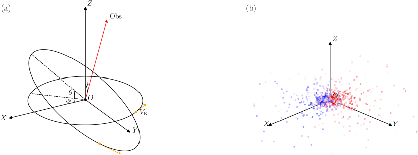
Figure 1: Illustration of the BLR model. (a) Coordinate system used in the present model. $O$ is the central black hole and $O-XY$ is equatorial plane of the BLR. A remote observer with an inclination of $i$ to the $OZ$-axis is located in the $O-YZ$ plane. All clouds are on circular orbits around the central black hole with Keplerian velocities $V_{\rm K}$. Two ellipses in the fugure show two possible orbits, and the orange arrow represents the velocity of a cloud at that position. $\theta$ is the angle between the orbital plane and the equatorial plane, and $\cos\theta$ is uniformly distributed between $[\cos\theta_{\rm opn},1]$, where $\theta_{\rm opn}$ is the half opening angle of the BLR. $\phi$ is the azimuthal angle of the orbital plane and uniformly distribute between $[0,2\pi]$. (b). Distribution of clouds generated for a typical BLR. Colors of clouds represent line of sight velocities. The observer’s line of sight is perpendicular to the paper. Clouds with red color are moving away from the observer while those with blue color towards the observer. There is an obvious velocity gradient in space, which is crucial for SA observations.

Over the past few decades, a sample of more than 100 AGNs with RM observations have advanced our understanding of BLRs a lot (Peterson et al., 1998; Kaspi et al., 2000; Bentz et al., 2013; Du et al., 2018). Particularly, geometries and dynamics of BLRs can be well studied through velocity-resolved delay maps obtained by RM (Grier et al., 2013). A disk-like BLR is common in many broad line Seyfert 1 galaxies (Bentz et al., 2013; Grier et al., 2013; Lu et al., 2016; Du et al., 2016; Xiao et al., 2018), even in some narrow-line Seyfert 1 galaxies (Du et al., 2016). Multiple RM observations of several objects, such as NGC 5548, 3C 390.3, and NGC 7469, show that the FWHM of H$\beta$ line and its lag $\tau_{\rm H\beta}$ follows $\tau_{\rm H\beta}\propto{\rm FWHM}^{-1/2}$, indicating Keplerian rotation of the BLR gas (Peterson et al., 2004). A flattened disk-like BLR in 3C 273 has also been detected by GRAVITY. Disk-like BLR with Keplerian rotation could be common.

Parameterized BLR model has been applied widely in RM data fitting in order to obtain physical quantities, such as BLR size and black hole mass, in a self-consistent way (Pancoast et al., 2014b; Li et al., 2018; Williams et al., 2018). A comprehensive model with $\sim 30$ parameters has been developed to include complex geometries and dynamics for perfect fitting of the observation data (Pancoast et al., 2014a). But as a preliminary guidance for SARM, we reasonably assume the Keplerian rotating disk model for the BLR, and include only the fundamental parameters for concise estimations of parameter impacts. This model also works quite well in Gravity Collaboration et al. (2018) and Wang et al. (2020) when fitting SA and SARM data of 3C 273, respectively.

The BLR is composed of a large amount of line-emitting clouds on circular orbits around the central black hole with Keplerian velocities, as shown in Fig. 1. The radial distribution of clouds is described by a shifted $\Gamma$-distribution. The distance of BLR clouds to the SMBH is generated by

$$r=R_{\rm S}+\mathscr{F}R_{\rm BLR}+\Gamma_{0}\beta^{2}(1-\mathscr{F})R_{\rm BLR},$$ (1)

where $R_{\rm S}$ is the Schwarzschild radius, $R_{\rm BLR}$ is the mean radius, $\mathscr{F}=R_{\rm in}/R_{\rm BLR}$ is the fraction of the inner to the mean radius, $\beta$ is the shape parameter, and $\Gamma_{0}=p(x|\beta^{-2},1)$ is a random number drawn from a $\Gamma$-distribution

$$p(x|\alpha,x_{0})=\frac{x^{\alpha-1}\exp(-x/x_{0})}{x_{0}^{\alpha}\Gamma(\alpha)},$$ (2)

where $x_{0}$ is a scale factor ($x_{0}=1$ here), $\alpha=\beta^{-2}$ and $\Gamma(\alpha)$ is the $\Gamma$-function. Symbols and meanings of all free parameters used in the BLR model are summarized in Table 1.

Our model in this work differs a little with that in Gravity Collaboration et al. (2018) and Wang et al. (2020) in the orientation distribution of orbital planes. We assume that the cosine of the angle between the direction of orbital angular momentum and $Z$-axis is uniformly distributed over $[\cos\theta_{\rm opn},1]$ to reach a uniform distribution of clouds. In previous work, the angle between the direction of angular momentum and $Z$-axis is uniformly distributed over $[0,\theta_{\rm opn}]$, and so clouds will be accumulated near the equatorial plane. We make the change for a more well-defined definition of opening angles. Clouds are randomly distributed along a given orbit by assigning their orbital phases uniformly over $[0,2\pi]$.

Table 1: Parameters used in the BLR model

Parameters	Meanings	Prior ranges	Fiducial values	Simulation ranges
$D_{\rm A}{\rm(Mpc)}$	Angular distance	$[10,10^{4}]$	$42.555$
$i(\arcdeg)$	Inclination angle of the LOS	$[0,90]$	$25$	$[1,45]$
$\rm PA(\arcdeg)$	Position angle	$[0,360]$	$90$	$[0,360]$
$M_{\bullet}(M_{\sun})$	Supermassive black hole mass	$[10^{6},10^{9}]$	$2\times 10^{7}$
$R_{\rm BLR}{\rm(ld)}$	Mean linear size	$[1,10^{3}]$	$15$
$F$	Fractional inner radius	$[0,1]$	$0.25$	$[0.1,0.9]$
$\beta$	Radial distribution shape parameter	$[0,4]$	$1.5$	$[0.5,2.5]$
$\theta_{\rm opn}(\arcdeg)$	Half opening angle	$[0,90]$	$25$	$[1,45]$

2.2 Spectroastrometry

A detailed mathematical formulation of SA of BLR can be found in Rakshit et al. (2015) and Songsheng et al. (2019a). We summarize it here for reader’s convenience. For an interferometer with a baseline $\bm{B}$, the differential interferometric phase for a non-resolved source is

$$\phi_{*}(\lambda)=-2\pi\bm{u}\dotproduct[\bm{\epsilon}(\lambda)-\bm{\epsilon}(\lambda_{\rm r})],$$ (3)

where $\bm{u}=\bm{B}/\lambda$ is the spatial frequency, $\bm{\epsilon}$ is the photocenter of the source at wavelength $\lambda$, $\lambda_{\rm r}$ is the wavelength of a reference channel. Here the bold letters represents vectors. Given the surface brightness distribution $\mathcal{O}(\bm{\alpha},\lambda)$ of the source, we have

$$\bm{\epsilon}(\lambda)=\frac{\int\bm{\alpha}\mathcal{O}(\bm{\alpha},\lambda)\differential[2]{\bm{\alpha}}}{\int\mathcal{O}(\bm{\alpha},\lambda)\differential[2]{\bm{\alpha}}},$$ (4)

where $\bm{\alpha}$ is the angular displacement on the celestial sphere. For AGNs, $\mathcal{O}=\mathcal{O}_{\ell}+\mathcal{O}_{\rm c}$, where $\mathcal{O}_{\ell}$ and $\mathcal{O}_{\rm c}$ are the surface brightness distribution contributed by the BLR and continuum regions, respectively. Once the BLR model is set up, $\mathcal{O}_{\ell}$ can be calculated through

$$\mathcal{O}_{\ell}(\bm{\alpha},\lambda)=\int\frac{\Xi_{r}F_{\rm c}}{4\pi r^{2}}f(\bm{r},\bm{V})\variation(\bm{\alpha}-\bm{\alpha}^{\prime})\variation(\lambda-\lambda^{\prime})\differential[3]{\bm{r}}\differential[3]{\bm{V}},$$ (5)

where $\lambda^{\prime}=\lambda_{\rm cen}\gamma_{0}\left(1+\bm{V}\dotproduct\bm{n}_{\rm obs}/c\right)\left(1-R_{\rm S}/r\right)^{-1/2}$ is the shifted wavelength of the photon from the broad emission line centered at $\lambda_{\rm cen}$ by Doppler effect and gravitation, $\gamma_{0}=\left(1-V^{2}/c^{2}\right)^{-1/2}$ is the Lorentz factor, ${\bm{\alpha}}^{\prime}=\left[\bm{r}-\left(\bm{r}\dotproduct\bm{n}_{\rm obs}\right)\bm{n}_{\rm obs}\right]/D_{\rm A}$, $\bm{r}$ is the displacement to the central BH, $\Xi_{r}$ and $f(\bm{r},\bm{V})$ are the reprocessing coefficient and velocity distribution of the clouds at position $\bm{r}$ respectively, $F_{\rm c}$ is ionizing fluxes received by an observer, $\bm{n}_{\rm obs}$ is the unit vector pointing from the observer to the source and $D_{\rm A}$ is the angular size distance of the AGN. Introducing the fraction of the emission line to total ($\ell_{\lambda}$), we have

$$\bm{\epsilon}(\lambda)=\ell_{\lambda}\,\bm{\epsilon}_{\ell}(\lambda),$$ (6)

where

$$\bm{\epsilon}_{\ell}(\lambda)=\frac{\int\bm{r}\mathcal{O}_{\ell}\differential[2]{\bm{\alpha}}}{\int\mathcal{O}_{\ell}\differential[2]{\bm{\alpha}}},\quad\ell_{\lambda}=\frac{F_{\ell}(\lambda)}{F_{\rm tot}(\lambda)},\quad F_{\ell}(\lambda)=\int\mathcal{Q}_{\ell}\differential[2]{\bm{\alpha}},\quad F_{\rm tot}(\lambda)=F_{\ell}(\lambda)+F_{\rm c}(\lambda).$$

Differential phase curve (DPC) can be obtain by inserting Eq. (6), (5) and (4) into (3). If the DPC whose amplitudes are a few degrees can be measured with SA, the effective spatial resolution will be 100 times the resolution limit $\lambda/B$.

2.3 Reverberation mapping

A detailed mathematical formulation of one dimensional RM can be found in Li et al. (2013, 2018). We also summarize it here for reader’s convenience. Damped random walk (DRW) model is used to describe continuum variations in order to interpolate and extrapolate light curves of continuum (Kelly et al., 2009; Zu et al., 2013). We first express the continuum light curve $\bm{y}$ by $\bm{y}=\bm{s}+\bm{n}+\bm{E}q$, where $\bm{s}$ denotes the underlying signal of the variation, $\bm{n}$ represents the measurement noise, $q$ is the mean value of the light curve, and $\bm{E}$ is a vector whose elements are all $1$. In the DRW model, the covariance function between $s_{i}$ and $s_{j}$ is given by

$$S(t_{i},t_{j})=\sigma_{\rm d}^{2}\exp(-\frac{|t_{i}-t_{j}|}{\tau_{\rm d}}),$$ (7)

where $t_{i}$ and $t_{j}$ are time for signal $s_{i}$ and $s_{j}$, respectively, $\sigma_{\rm d}$ is the long-term standard deviation of the variation and $\tau_{\rm d}$ the typical timescale.

We further assume that both $\bm{s}$ and $\bm{n}$ are Gaussian and uncorrelated. Given $\bm{y}$, posterior distribution of $\sigma_{\rm d}$, $\tau_{\rm d}$ and $q$ can be obtained by Bayesian analysis with likelihood function

$$P(\bm{y}|\sigma_{\rm d},\tau_{\rm d},q)=\frac{1}{\sqrt{(2\pi)^{m}|\bm{C}|}}\exp\left[-\frac{(\bm{y}-\bm{E}q)^{T}\bm{C}^{-1}(\bm{y}-\bm{E}q)}{2}\right],$$ (8)

where superscript “$T$” denotes transposition, $\bm{C}=\bm{S}+\bm{N}$, $\bm{S}$ and $\bm{N}$ are the covariance matrix of $\bm{s}$ and $\bm{n}$ respectively, and $m$ is the number of data points.

Given parameters $(\sigma_{\rm d},\tau_{\rm d},q)$, a typical realization for the observed continuum light curve will be

$$f_{c}=(\bm{u}_{s}+\hat{\bm{s}})+\bm{E}(u_{q}-\hat{q}),$$ (9)

where $\hat{q}=\bm{E}^{T}\bm{C}^{-1}\bm{y}/\bm{E}^{T}\bm{C}^{-1}\bm{E}$, $\hat{\bm{s}}=\bm{S}^{T}\bm{C}^{-1}(y-\bm{E}\hat{q})$, and $\bm{u}_{s}$ and $u_{q}$ are Gaussian processes with zero mean and covariance matrices $\bm{Q}=(\bm{S}^{-1}+\bm{N}^{-1})^{-1}$ and $C_{q}=(\bm{E}^{T}\bm{C}^{-1}\bm{E})^{-1}$ respectively. Next, $\bm{u}_{s}$ and $u_{q}$ are treated as free parameters and further constrained by light curves of the emission line.

Given the BLR model and the realization of continuum light curves, the variation of the emission line is calculated by

$$f_{\ell}(t)=\int\differential{\bm{r}}\differential{t^{\prime}}\frac{\Xi_{r}f_{\rm c}(t^{\prime})}{4\pi r^{2}}n(\bm{r})\delta\left(t^{\prime}-t+\tau\right),$$ (10)

where $\tau=(r-\bm{r}\dotproduct\bm{n}_{\rm obs})/c$, $\Xi_{r}$ is the reprocessing coefficient and $\bm{n}(\bm{r})$ is the number density of the clouds.

2.4 Joint analysis

The goal of a fully joint analysis is to obtain the posterior probability distribution of the model parameters consistently using the combined data from SA and RM observations. SA and RM observations are conducted independently, thus we assume that the probability distribution for the measurement errors of light curves, profiles and DPCs are uncorrelated. The joint likelihood function can be written as

$$P(\mathscr{D}|\bm{\Theta}) =\displaystyle\prod_{i=1}^{N_{\rm RM}}\frac{1}{\sqrt{2\pi\sigma_{\ell}^{2}}}\exp\left\{-\frac{\left[f_{\rm\ell,obs}-f_{\rm\ell,mod}\left(f_{\rm c,obs}|\bm{\Theta}\right)\right]^{2}}{2\sigma_{\ell}^{2}}\right\}\times\prod_{i=1}^{N_{\rm G}}\prod_{j=1}^{N_{\lambda}}\frac{1}{\sqrt{2\pi\sigma_{\phi_{ij}}^{2}}}\exp\left\{-\frac{\left[\phi_{\rm obs}-\phi_{\rm mod}\left(\bm{\Theta}\right)\right]^{2}}{2\sigma_{\phi_{ij}}^{2}}\right\}$$ (11)

$$\displaystyle\times\prod_{j=1}^{N_{\lambda}}\frac{1}{\sqrt{2\pi\sigma_{\rm F}^{2}}}\exp\left\{-\frac{\left[F_{\rm\ell,obs}-F_{\rm\ell,mod}\left(\bm{\Theta}\right)\right]^{2}}{2\sigma_{\rm F}^{2}}\right\},$$

where $\mathscr{D}$ represents the data set, $\bm{\Theta}$ represents all the model parameters, $f_{\rm c,obs}$ is the continuum data, $f_{\rm\ell,obs}$, $F_{\rm\ell,obs}$, and $\phi_{\rm obs}$ are the line flux, line profile, and DPC of the emission line with measurement uncertainties $\sigma_{\ell}$, $\sigma_{\phi_{ij}}$ and $\sigma_{\rm F}$ respectively, and $(f_{\rm\ell,mod},F_{\rm\ell,mod},\phi_{\rm mod})$ are the corresponding predicted values from the BLR model.

In light of Bayes’ theorem, the posterior probability distribution for $\bm{\Theta}$ is given by

$$P(\bm{\Theta}|\mathscr{D})=\frac{P(\bm{\Theta})P(\mathscr{D}|\bm{\Theta})}{P(\mathscr{D})},$$ (12)

where $P(\bm{\Theta})$ is the prior distribution of the model parameter and $P(\mathscr{D})$ is a normalization factor. DNest algorithm can be applied to sample the distribution Eq. (12). A brief introduction to the DNest algorithm is given in Appendix C.

3 Results

3.1 Impacts of data qualities

Figure 2: Relative uncertainties and bias of part of model parameters under different SA data qualities. The mock data of SA and RM are both generated by the BLR model of the same parameter values shown in Table 1. Relative errors of RM data are fixed, while those of SA data are varied to be $5\%$, $10\%$, $20\%$ and $40\%$. The configuration of baselines follows the SA observation of 3C 273. So the target is observed four times for SA data.

SARM data consists of light curves of optical continuum and emission lines, profiles of NIR emission lines as well as its DPC. Observation of light curves and line profiles are relatively mature and data quality for most SARM targets can be quiet good. On the contrary, techniques for obtaining DPCs are still in development, and data quality largely depends on seeing and target brightness. In this subsection, we mainly study the impact of DPC data quality on the measurement of distance, black hole mass and BLR geometry.

To generate typical mock data, we take the fiducial values in Table 1 for the BLR model. The light curves of continuum and emission line last for 200 days with 1 day cadence. The continuum light curves are generated by the DRW model with $\tau_{\rm d}=60{\rm\,d}$ and $\sigma_{\rm d}=0.25$. The relative errors of continuum and line variations are $0.5\%$ and $1\%$, respectively. We generate mock RM data with higher qualities than those in typical RM campaigns in order to focus on impacts of data qualities of SA observations on distance measurements. The redshift of the target is assumed to be $0.01$, and the NIR emission lines for SA is Brackett $\gamma$ (Br$\gamma$) centered at $2.166{\rm\,\mu m}$ in rest frame. The equivalent width of Br$\gamma$ is $40$ Å. We follow the spectral resolution of GRAVITY ($\lambda/\Delta\lambda\sim 500$) and broaden the profile by a Gaussian with ${\rm FWHM}=4{\rm\,nm}$ ($\sim 600\rm km\,s^{-1}$). The relative error of the profile is $0.5\%$. The configuration of baseline we used for generating DPC is the same as that of Extended Data Fig. 1 (b) in Gravity Collaboration et al. (2018) (which means the target is observed four times in total). We also assume the absolute error of phase isthe same in all wavelength channels and baselines for simplification.

To quantify data qualities of DPCs, we define the relative error as the ratio of phase error to the peak of DPCs with largest amplitudes. We vary the relative error of DPC to be $5\%$, $10\%$, $20\%$ and $40\%$. For each data set, we obtain the posterior probability distribution of model parameters through Bayesian analysis introduced in subsection 2.4. An example of generation and fitting of mock data is illustrated in Appendix A.

We define inferred value of the model parameters as median of the posterior distribution, and lower/upper bound as $16\%$ and $84\%$ quantile. Uncertainty of the parameters are defined as half of the difference between the upper and lower bounds and bias as the difference between the inferred and input value. Finally, for dimensional quantities, we divide the uncertainty by inferred value and bias by input value to get the relative uncertainty and bias; for angles, we divide them by $1{\rm rad}$ instead. We emphasis here that bias is not systematic uncertainty. It is the deviation of inferred values of model parameters from input ones caused by finite width of posterior probability distribution (uncertainty). The absolute value of bias is comparable to uncertainty usually. A much larger bias than uncertainty indicates the fail of Bayesian analysis, mostly caused by degeneracy between model parameters.

Relative uncertainties and bias of part of model parameters under different SA data qualities are shown in Fig. 2. As we can see in upper panel of Fig. 2(a), relative uncertainties of $R_{\rm BLR}$ are $2.58\%$ and independent of errors of DPCs, since it is only constrained by light curves of continuum and emission lines. Uncertainties of $\rm PA$ are proportional to errors of DPCs and the proportional coefficient is approximately $0.14$. Since $D_{\rm A}=R_{\rm BLR}/\xi_{\rm BLR}$, where $\xi_{\rm BLR}$ is the mean angular size, we have

$$\delta_{D_{\rm A}}=\sqrt{\delta_{R_{\rm BLR}}^{2}+\delta_{\xi_{\rm BLR}}^{2}},$$ (13)

where $\delta_{x}$ means the relative uncertainty of $x$. If we assume $\delta_{\xi_{\rm BLR}}=k\delta_{\rm DPC}$ and let $\delta_{R_{\rm BLR}}=2.58\%$, we can get through fitting

$$\delta_{D_{\rm A}}=\sqrt{(2.58\%)^{2}+(0.23\delta_{\rm DPC})^{2}}.$$ (14)

We must emphasis that this relation is valid only for this set of parameters, since relative uncertainties of $D_{\rm A}$ also depends on inclinations and opening angles, as shown in the next subsection. There are no systematic uncertainties for mock data analysis, but they should be considered in real observations.

Lower panel of Fig. 2(a) presents the relation between bias and data error. Median values of posterior distributions are obtained with greater randomness than uncertainties, leading to a more irregular pattern. The bias of $R_{\rm BLR}$ changes little with data error, while the bias of $D_{\rm A}$ increases with data error, in agreement with results in the upper panel. The bias of $\rm PA$ fluctuates when $\delta_{\rm DPC}\leq 20\%$, but increases a lot when $\delta_{\rm DPC}=40\%$.

Figure 3: Probability density distributions of black hole mass $M_{\bullet}$, half opening angle $\theta_{\rm opn}$ and inclination angle $i$. The median values of the parameters are given on the tops of panels. Error bars are quoted at the 1$\sigma$ level, which are given by each distribution. The blue lines represent input values. The dashed lines in the one-dimensional distributions are the 16%, 50% and 84% quantiles, and contours are at $1\sigma$, $1.5\sigma$ and $2\sigma$ respectively. As we can see, strong correlation between $M_{\bullet}$, $i$ and $\theta_{\rm opn}$ can lead to large bias when fitting. The figure is plotted using the corner module developed by Foreman-Mackey (2016).

As shown in Fig. 2(b), for $M_{\bullet}$, $i$ and $\theta_{\rm opn}$, there is no systematic change of uncertainty or bias when error of DPC data varies, because these parameters are mainly constrained by profiles of emission lines. But we note that there is a dramatic increase of bias for $M_{\bullet}$ when $\delta_{\rm DPC}=20\%$. It may be caused by strong correlation between $M_{\bullet}$, $i$ and $\theta_{\rm opn}$, as shown in Fig. 3. The correlation comes from the fact that the FWHM of the emission line can remain unchanged if we increase black hole mass and decrease opening or inclination angle simultaneously. In the case of strong correlation, input values have exceeded $1\sigma$ range in 1 dimensional distributions, though they are still on the boundary of $1\sigma$ range in 2 dimensional distributions. Furthermore, the sampling algorithm we used also performs worse when correlations between parameters get stronger. Thus, strong correlation between parameters can lead to large bias in fitting.

3.2 Amplitudes of DPCs

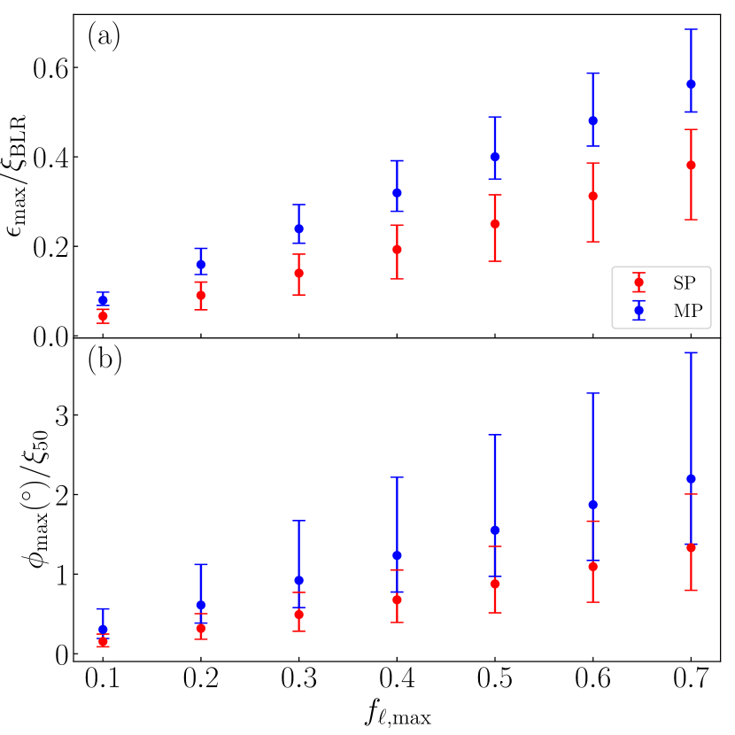
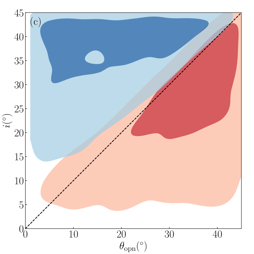
Figure 4: (a)The ratio of photocenter displacement to average angular size of BLR under different emission line strength in our simulated sample. It is evidently that photocenters of targets with multiple peaks in their profiles are lager than those with single peaks. (b) Predicted amplitudes of differential phases observed by GRAVITY. Here, we assume that average angular sizes of BLRs are $50{\rm\,\mu as}$ ($\xi_{50}=\xi_{\rm BLR}/50{\rm\,\mu as}$) and targets are at the zenith when observed. Ranges of phase amplitudes for targets with multiple peaks in their profiles and those with single peaks partially overlap due to the large uncertainties of position angles. (c) Distribution of inclination and opening angles for objects with single (red region) and multiple (blue region) peaks in profiles respectively. The dark and light color represents $1\sigma$ and $2\sigma$ levels respectively. When $i>\theta_{\rm opn}$, profiles usually possess multiple peaks.

In order to estimate the precision of distance measurement for a sample of targets, we need to predict amplitudes of DPCs for given magnitudes, redshifts and profiles of emission lines. From Eq. 3, the differential phase depends on the photocenter $\bm{\epsilon}(\lambda)$ of the target as well as its projection to the baseline $\bm{B}$ of the interferometer.

Given the redshift of an AGN, its angular and luminosity distance can be estimated easily using current values of cosmological parameters. The luminosity of the AGN can then be obtained from its magnitude. The widely used $R-L$ relation (Bentz et al., 2013) (but see Du & Wang (2019) for its revised version) now comes in and predicts the average size of the BLR. However, a small inclination angle or large opening angle would make the system more symmetric, leading to a photocenter displacement much smaller than the average angular size of the BLR. Meanwhile, when the emission line is weak compared to the continuum, the peak of $\bm{\epsilon}(\lambda)$ will decrease significantly from Eq. 6.

In order to quantify all these effects, we choose $i$, $\theta_{\rm opn}$, $F$ and $\beta$ randomly from the ranges shown in Table 1 to generate a large sample of $\bm{\epsilon}_{\ell}(\lambda)$ and corresponding line profiles. Dimensional parameters $D_{\rm A}$, $R_{\rm BLR}$ and $M_{\bullet}$ will be fixed since they can only change the overall amplitude and width rather than the shape of the DPC and profile. We divide the sample into two categories according to the number of peaks in their line profiles. For each category, we calculate the median value and $1\sigma$ limit of the ratio $\epsilon_{\rm max}/\xi_{\rm BLR}$ under different $f_{\rm\ell,max}$, where $\xi_{\rm BLR}$ is the average angular size of the BLR, and $\epsilon_{\rm max}$ and $f_{\ell,max}$ are the maximum value of $|\bm{\epsilon}(\lambda)|$ and $f_{\ell}(\lambda)$ respectively. The result is shown in Fig. 4(a). Clearly, the displacement of photocenter is roughly proportional to the ratio of line flux to total flux at line center, and photocenters of targets with multiple peaks in their profiles are systematically lager than those with single peaks.

In order to predict the peak amplitude of actual phase signal, we must know the projected base line configuration and position angle of the target. For simplicity, we assume targets are at the zenith when observed and the configuration of baselines are the same as that of VLTI. Position angles of targets are uniformly distributed between $0\arcdeg$ and $360\arcdeg$. The result is shown in Fig. 4(b). Similarly, phase amplitudes of targets with multiple peaks in their profiles are larger than those with a single peak.

3.3 Impacts of inclination and opening angles

Figure 5: Relative uncertainties and bias of part of model parameters under different inclinations and opening angles. The mock data of SA and RM are both generated by the BLR model of the same parameter values shown in Table 1 except inclinations and opening angles. Relative errors of SARM data are fixed. The configuration of baselines follows the observation of 3C 273. So the target is observed four times for SA data.

Even if the data qualities are the same, uncertainties and accuracies of distance measurements can vary with shapes of DPCs and profiles. Dimensional parameters $D_{\rm A}$, $R_{\rm BLR}$ and $M_{\bullet}$ can only change the overall amplitude and width rather shape of the DPC and profile. Their impacts on the distance measurement can be converted to impacts of relative error of the data. Among remaining parameters, $i$ and $\theta_{\rm opn}$ can change the shape of the DPC and profile drastically (Rakshit et al., 2015; Songsheng et al., 2019b), thus altering degeneracies among all parameters, consequently further changing the uncertainty of parameter inference. In order to study their impacts, we vary $i$ and $\theta_{\rm opn}$ from $5\arcdeg$ and $45\arcdeg$ respectively, and keep other parameters the same as those in subsection 3.1 and relative error of the DPC at $20\%$. For each data set, we perform the Bayesian analysis and calculate relative uncertainty and bias for each parameter. The results are shown in Fig. 5.

Generally, uncertainties of $D_{\rm A}$ becomes large when $i$ decreases, as illustrated in Fig. 5(a). For low inclinations (such as $i\lesssim 10\arcdeg$), the profile of broad emission line usually posses a single peak (slightly depends on opening angles), as shown in Fig.4(c). In this case, the inclination is hard to be determined accurately due to degeneracies with other parameters. Furthermore, the LOS approaching the symmetry axis will significantly increase the symmetry of the system, thus decrease the amplitude of DPC drastically. Thus, the correlation between $i$ and $D_{\rm A}$ becomes much stronger, as shown in Fig. 6, leading to larger uncertainties of $D_{\rm A}$.

For moderate inclinations ($i\sim 15\arcdeg-25\arcdeg$), uncertainties of $D_{\rm A}$ also increase with opening angles of BLRs due to increasing symmetries. There are obvious leaps of correlations between $D_{\rm A}$ when $\theta_{\rm opn}=25\arcdeg(i=15\arcdeg)$ or $\theta_{\rm opn}=35\arcdeg(i=25\arcdeg)$, since profiles become single-peaked when $\theta_{\rm opn}>i$. If inclinations become larger ($i\sim 35\arcdeg-45\arcdeg$), systems will keep asymmetry and degeneracies between $D_{\rm A}$ and $i$ are weak, contributing to much smaller uncertainties of $D_{\rm A}$.

The variation of the $D_{\rm A}$-bias with inclinations and opening angles is roughly similar. We emphasis that the Bayesian inference becomes very unstable for a system with low inclinations and large opening angles because the system will be highly symmetric in the view of the observer. In such a case, extremely large biases $(\geq 100\%)$ appear, even much larger than uncertainties, and the inferred value of distance can not be trusted.

Figure 6: Pearson product-moment correlation coefficients of angular distances and inclination angles under different inclinations and opening angles. Generally, the smaller the inclination angle, the stronger the correlation between the distance and the inclination angle. For moderate inclination angles ($i\sim 15\arcdeg-25\arcdeg$), correlations also increase with opening angles of BLR. Correlation coefficients are calculated through corrcoef method in python’s numpy module.

In Fig. 5(b), the evolution of the uncertainty of $i$ with opening angles is similar to that of $D_{\rm A}$. There is no systematic increase of $\delta_{i}$ as $i$ decreases since our definition of $\delta_{i}$ is $\Delta i/{\rm 1\,rad}$ rather than $\Delta i/i$. In Fig. 5(c), uncertainties of $\rm PA$ measurements increase slightly when inclinations decrease, but they can be determined much more accurately compared to other parameters. In Fig. 5(d), uncertainties of measurements of $M_{\bullet}$ also tend to be large for face-on targets, since a slight change of $i$ can cause a significant variation of width of DPC or profile when inclination is small. In Fig. 5 (e), inference of $R_{\rm BLR}$ is less affected by the inclination and opening angle, as one dimensional RM is insensitive to them. In Fig. 5 (f), uncertainties of $\theta_{\rm opn}$ vary with inclinations and opening angles similarly to those of $i$ due to correlations between $i$ and $\theta_{\rm opn}$. Generally, values of $\Delta i$ and $\Delta\theta_{\rm opn}$ are relatively close.

4 Discussion

4.1 Error budget

Figure 7: The ratio between the relative uncertainty of angular size of BLR and that of DPC ($\alpha$) under different inclinations and opening angles. For very small inclinations ($i\sim 5\arcdeg$), the relative uncertainty of angular size of BLR is twice that of DPC, while for large inclinations ($i\sim 35\arcdeg-45\arcdeg$), it is less than half of the DPC.

The statistical relative uncertainties of distance measurements can be written as

$$\delta_{D_{\rm A}}=\sqrt{\delta_{R_{\rm BLR}}^{2}+\alpha^{2}\delta_{\rm DPC}^{2}},$$ (15)

where the coefficient $\alpha$ depends on inclination and opening angles of BLRs. Multiple observations ($N$) of a target can significantly reduce the statistical uncertainty. Considering these influences, we have

$$\delta_{D_{\rm A}}=\sqrt{\delta_{R_{\rm BLR}}^{2}+\alpha^{2}\delta_{\rm DPC}^{2}/N}.$$ (16)

From simulations shown in Fig. 5, we can estimate the value of $\alpha$ for different inclination and opening angles . The result is shown in Fig. 7. When the inclination is very small ($i\sim 5\arcdeg$), the $\alpha$ is around $2$, and the bias of inference is too large to obtain a credible measurement. For moderate inclinations, ($i\sim 15\arcdeg-25\arcdeg$), we have $\alpha\sim 0.5$ when $i\gtrsim\theta_{\rm opn}$ and $\alpha\sim 1.5$ when $i\lesssim\theta_{\rm opn}$. For large inclinations, ($i\sim 35\arcdeg-45\arcdeg$), the $\alpha$ is about $0.4$.

Inclinations and opening angles can be in principle inferred through number of peaks in line profiles. As shown in Fig 4(c), if inclinations are large and opening angles are small ($i>\theta_{\rm opn}$), simulated profiles usually possess multiple peaks, and vice versa. So selecting objects with multiple peaks in their profiles can reduce uncertainties in distance measurements notably. In practice, due to the blend of narrow line emission and instrument broadening effect, the proportion of objects with multiple peaks in profiles in real samples is much smaller than that in our simulated samples (e.g., see Liu et al., 2019, Table  2). A quick way to estimate inclinations and opening angles of a large sample of objects is to compare their profiles with template profiles simulated by BLR models. Objects with $i<10^{\circ}$ or $\theta_{\rm opn}>40^{\circ}$ can be excluded at first step. Before making observation plans, we can fit profiles of specific objects to the BLR model to obtain a reliable estimation for inclination and opening angles (e.g., Raimundo et al., 2019, 2020). Then we can predict the expected DPC for each object and choose appropriate ones for SARM campaign. Other ways to determine inclinations of AGNs includes narrow line region kinematics (Fischer et al., 2013) and pc-scale radio jet (e.g. Kun et al., 2015).

Systematic errors of distance measurement through SARM have been discussed thoroughly in Wang et al. (2020). Firstly, RM campaign measures the region of optical emission line (usually $\rm H\beta$ for objects with low redshifts) while SA conducted by GRAVITY can only measure the region of NIR emission line (usually $\rm Br\gamma$ or $\rm Pa\alpha$). Their size may be sightly different due to the different optical depths. But this can be reduced by comparing widths of different emission lines in joint analysis of velocity-resolved RM and SA observations. For 3C 273, the difference between the size of $\rm H\beta$ and $\rm Pa\alpha$ emitting region is estimated to be $13\%$, which is slightly smaller than the statistical error. A RM campaign using the same emission line as that in SA observation are highly needed to quantify this effect. Secondly, RM campaign measures the variable part of a BLR while SA observes the entire region, resulting in systematic errors in the SARM analysis. By comparing the shape and width of mean with root-mean-square (RMS) spectra across the whole RM campaign, the error can also been assessed. For 3C 273, the variable part of its BLR show little difference with the entire BLR. Finally, signatures of inflow or outflow has been found recently by analysing high-quality RM data (Pancoast et al., 2014b; Grier et al., 2013; Xiao et al., 2018). The general shape of differential phase curve for an inflow BLR is similar to that of a Keplerian BLR, except that the displacement of photocenter would be parallel to the axis rather than perpendicular to it (Rakshit et al., 2015). The angular size of BLR can still be well constrained by SA observation, and so the uncertainty of distance through SARM analysis will not change a lot. However, the relation between clouds’ velocities and black hole mass will be much more ambiguous, increasing the uncertainty of black hole mass measurement. Based on these limited information and the fact that angular distance of 3C 273 measured by SARM is consistent with that from the current cosmological model, we draw a conclusion that systematic errors are at most comparable to statistical errors.

4.2 Model tests

In our mock data analysis, the correctness of BLR model is always guaranteed and the all fittings can reach $\chi^{2}\approx 1$ level. However, BLRs are diverse individually. Our simplest model works quite well for 3C 273 since its profile of emission line are symmetric. When selecting targets, objects with simple and regular line profiles should be prioritized. The response of emission line to continuum also needs to be clear to avoid complications by long term trending, BLR ”holiday”, multiple lags or fast breathing. Before Bayesian analysis, model-independent methods, such as reconstruction of velocity-delay map through maximum entropy method or calculation of centroid position of the photocenter in several wavelength channels, should be applied to obtain the basic geometry and dynamics of the BLR. The appropriate model with minimum number of parameters will be tested first. Subsequently, more can be added until a good fitting reaches.

Actually, radial distribution of BLR clouds described by Eq. (1, 2) can be alternatively assumed by other forms, such as Gaussian distributions (Pancoast et al., 2011). This leads to different results of distances from the fittings, which could be regarded as one of systematical errors. This can be addressed by evaluating the Bayesian evidence of the model, which is a prime result of nested sampling method (Skilling, 2006; Shaw et al., 2007). Moreover, SMBH mass can be simultaneously obtained by the SARM analysis. We will discuss these issues in an separate paper.

4.3 $H_{0}$-tension

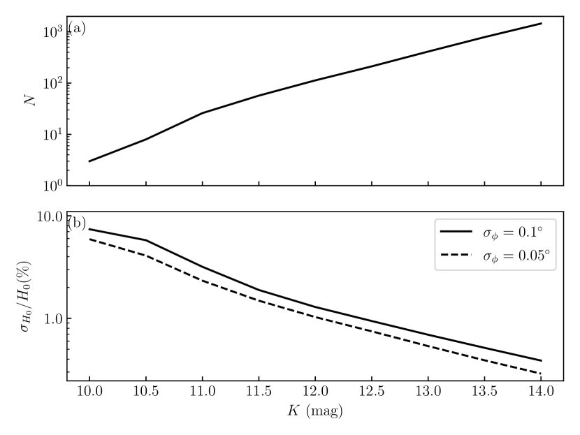
Figure 8: (a) The expected number of Type I AGNs which can be observed using GRAVITY as the limiting $K$ band magnitude increases. (b) The corresponding $H_{0}$ measurement error through SARM, assuming each object are observed four times. $\sigma_{\phi}$ is the uncertainties of phase in each observation for each base line. The uncertainties of linear size of BLR through RM are kept at $10\%$. Systematical error bars risen from the different lines between RM and SA observations can be inprinciple alleviated by either mapping the same line with SA or through kinematic relation of the SARM lines.

Since the beginning of the last century, advances in the distance measurement of extragalactic objects have been driving the development of cosmology. In particular, the cosmic distance ladder using Cepheid and Type Ia supernovae as standard candles has made great achievements, including the discovery of the expansion of the universe (Hubble, 1929) as well as its acceleration (Riess et al., 1998; Perlmutter et al., 1999). Currently, the Equation of State of Dark energy (SH0ES) program achieves a measurement of the Hubble constant ($H_{0}$) with $1.91\%$ precision based on the distance ladder, providing a value of $H_{0}=74.03\pm 1.42{\rm\,km\,s^{-1}\,Mpc^{-1}}$ (Riess et al., 2019). However, observations of the cosmic microwave background (CMB) radiation from the early universe enables an indirect inference of $H_{0}$ under the assumption of the flat $\Lambda$CDM cosmological model, giving $H_{0}=67.4\pm 0.5{\rm\,km\,s^{-1}\,Mpc^{-1}}$ (Planck Collaboration et al., 2018). Tensions between the early and late Universe measurements are at the level of $\sim 4.4\sigma$ (Verde et al., 2019), indicating that either unaccounted systematic errors might bias at least one of these measurements (see discussion of its possibility in Davis et al., 2019; Rameez & Sarkar, 2019; Rose et al., 2020), or the flat $\Lambda$CDM cosmological model needs to be extended to include new physics, such as dynamical/interacting dark energy (e.g., Di Valentino et al., 2016, 2017; Huang & Wang, 2016; Zhao et al., 2017), dark radiation (e.g., Buen-Abad et al., 2015; Ko & Tang, 2016), neutrino self-interaction (e.g., Blinov et al., 2019; Kreisch et al., 2020), and so on.

At such a cross roads, new approaches to determining Hubble constant without calibration of the local distance ladders or assumption of the flat $\Lambda$CDM cosmological model are particularly important as arbitrators. Gravitational wave emitted by binary neutron star merger can be used as “standard siren” to determine the luminosity distance of the binary Schutz (1986). The recent observation of the merger signal GW180817 (Abbott et al., 2017a) along with its optical counterpart (Abbott et al., 2017b; Soares-Santos et al., 2017) provided the first standard siren measurement of $H_{0}$ with precision $14\%$ (Abbott et al., 2017c). Its constraint ability of cosmological parameters, including Hubble constant, has been extensively studied (Cai & Yang, 2017; Chen et al., 2018). Another promising approach relies on strong gravitational lenses with measured time delays between the multiple images (Refsdal, 1964). The program $H_{0}$ Lenses in COSMOGRAIL’s Wellspring (H0LiCOW) (Suyu et al., 2017) obtained a $2.4\%$ measurement of $H_{0}$ from a joint analysis of six gravitationally lensed quasars, in agreement with measurements of $H_{0}$ by the local distance ladder (Wong et al., 2020).

Systematic errors caused by BLR size discrepancy of different emission lines are not included in Fig 8, making it an optimistic estimation of $H_{0}$ constraints by SARM project. However, if we use the velocity resolved RM data by including profiles of optical emission lines, BLR sizes of optical and NIR lines can be different in the model. The systematic errors can be alleviated.

In order to study the constraint ability on $H_{0}$ by joint analysis of SARM data, we generate a mock sample of type I AGNs for GRAVITY/GRAVITY+. Details on the generation and properties of the sample are presented in Appendix B. For each object in the sample, the profile and DPC are simulated using BLR models. Once we obtain the maximum amplitudes of phase curves $\phi_{\rm max}$, uncertainties of distance measurements for each object can be estimated by Eq. 16. If other cosmological parameters are fixed except $H_{0}$, the uncertainty of $H_{0}$ measurement using the whole sample can be obtained.

Since 200 day light curves with 1 day cadence and no gaps can hardly be achieved in typical RM campaigns, we would assume the relative uncertainty of BLR size measurement through RM campaign is $10\%$ rather than $2\%$ shown in Fig. 2(a). (e.g., a recent RM campaign conducted by Bentz et al. (2021) for NGC 3783, which is also a suitable target for GRAVITY, obtained a time lag measurement with $10\%$ uncertainty.) We also assume the uncertainty of phase measurement for each baseline is $0.1\arcdeg$. Note that highly face-on objects ($i\lesssim 10\arcdeg$) are discarded due to their large biases in distance measurements. Objects with maximum phases less than $0.1\arcdeg$ are also excluded since they help little to constrain the Hubble constant.The result is shown in Fig 8. As we can see, by observing $60$ targets with $K$ band magnitudes better than $11.5$ and maximum phase larger than $0.1\arcdeg$ through GRAVITY, the uncertainty of $H_{0}$ will be less than $2\%$. Currently, GRAVITY can achieve a phase error of $0.1\arcdeg$ per baseline in observations of bright ($K\sim 10-11$) AGNs (Gravity Collaboration et al., 2018; GRAVITY Collaboration et al., 2020; Dexter et al., 2020). But the integration time for each object may reach 10 hours due to the limit of fringe tracking. Fortunately, GRAVITY+, the upgraded version of GRAVITY, aims to achieve on-axis fringe tracking for AGNs as faint as $K\sim 14-15$ in the near future (Dexter et al., 2020). If we assume that GRAVITY+ requires $1-2$ hour of integration time to reach a phase error of $0.1\arcdeg$ per baseline for these bright targets, $60-120$ hours of observation time can measure the Hubble constant with better than $2\%$ accuracy.

Finally, we would like to point out that a sample composed of 53 AGNs for future SARM campaigns has been selected by Wang et al. (2020) from the current catalogs (mainly from Veron-Cetty and Verson’s catalog, and 2dF and 6dF ect). AGNs surveyed by 4MOST in future will be greatly increased in the southern hemisphere, moreover powerful GRAVITY+ onboard VLTI will conveniently observe fainter AGNs and quasars at cosmic noon between $z=2-3$, offering opportunities of measuring cosmic expansion history from local Univerise to the deeper.

5 Conclusion

In this paper, we conduct a mock data analysis for cosmology through SARM campaign. We have tested how the relative uncertainties of distance measurements depend on errors of DPCs as well as the roles of inclinations and opening angles of broad-line region (BLR). For BLRs with inclinations $\gtrsim 10\arcdeg$ and opening angles $\lesssim 40\arcdeg$, analyses of SARM data can generate reliable quasar distances even for relatively poor SA measurements with relative error of $40\%$ for GRAVITY-like facilities. If the limiting magnitude of the GRAVITY reaches $11.5$ in $K$ band and errors of phase measurements are as low as $0.1\arcdeg$, the SARM campaign can constrain $H_{0}$ to an uncertainty of $2\%$ by observing $60$ targets.

Appendix A Mock data

Here, we present an example of mock data generation and its fitting for illustration. We use the parameterized BLR model describe in subsection 2.1, and values of its parameters are taken to be the fiducial values listed in Table 1. The continuum variation is generated by the DRW model with timescale $\tau_{\rm d}=60{\rm\,d}$ and amplitude $\sigma_{\rm d}=0.25$. Then it is convolved with the velocity-resolved transfer function determined by BLR model to obtain the light curve of emission line. Both light curves are sampled with $1$ day cadence and last for $200$ days. The relative uncertainties of each data point are $0.5\%$ for continuum and $1\%$ for emission line. Blue points with errorbars in Fig 9 are mock light curves we generated.

The profile and DPCs are simulated using the same BLR model. The emission line used for SA is Br$\gamma$. To normalize the profile, we assume the equivalent width of the line is $40\text{\AA}$ in rest frame. The redshift of the object is $0.01$, shifting the central wavelength of the Br$\gamma$ to $2.18766{\rm\,\mu m}$. There are $40$ wavelength bins between $2.14$ and $2.24{\rm\,\mu m}$, and the profile and DPC are broadened by a Gaussian with ${\rm FWHM}=4{\rm\,nm}$. The relative uncertainty of the profile and DPC are $0.5\%$ and $20\%$ respectively. The object is observed for four times with six baselines, and the configuration of baselines is the same as that of Extended Data Fig. 1 (b) in Gravity Collaboration et al. (2018). Points with errorbars in Fig 10 are mock profile and differential phase curves we generated.

Bayesian analysis is applied to fit the combined mock data jointly to the BLR model and obtain the posterior probability distribution of model parameters, as described in subsection 2.4. DNest algorithm is used to sample the posterior distribution 12 (Brewer & Foreman-Mackey, 2018; Li, 2020), generating a posterior sample of model parameters and associated light curves, profile and DPCs. The reconstructed curves with smallest $\chi^{2}$ (the best fitting) are thick solid lines shown in Fig 9 and 10, while those randomly drawn from the posterior sample are thin gray lines.

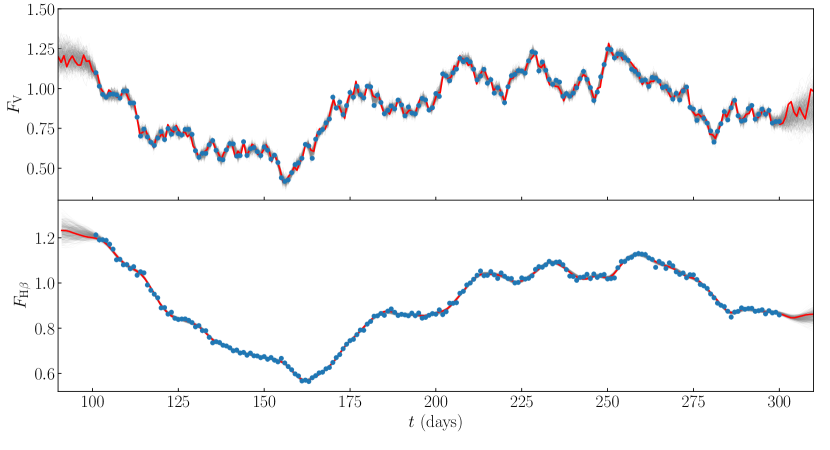
Figure 9: An example of mock light curves we generated and its fitting to the BLR model. The first row is continuum variation and the second is emission line variation. Error bars for data points reflect 1 $\sigma$ uncertainties. The thick red lines are the best fitting, while the thin gray  lines are fittings using model parameters drawn from the probability distribution of model parameters.

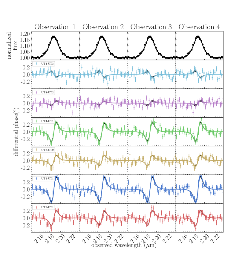
Figure 10: An example of mock profile and DPC we generated and its fitting to the BLR model. The first row is the Br$\gamma$ profile, and the second to the last rows are corresponding DPCs for each baseline. The object is observed for four times. Error bars for data points reflect 1 $\sigma$ uncertainties. The thick solid lines are the best fitting while the thin gray lines are fittings using model parameters drawn from the probability distribution of model parameters.

Appendix B Mock sample

In order to study the constraint ability on $H_{0}$ by joint analysis of SARM data from a large sample of type I AGNs, we need to generate a mock sample using realistic luminosity functions of quasars. We first divide the redshift (up to $z=1$) and bolometric luminosity (from $10^{41.6}$ to $10^{51.5}{\rm erg\,s^{-1}}$) into short bins. Then we estimate the number of quasars in each bin using the redshift-dependent bolometric quasar luminosity function in Hopkins et al. (2007). Assuming the inclination of AGNs are isotropic and broad emission line can be observed when $i<45\arcdeg$, only $29.3\%$ of them are type I. The distribution of AGNs on celestial sphere is also isotropic. When the difference between the declination of the target and latitude of VLTI is smaller than $45\arcdeg$, the object can be observed by GRAVITY. Thus, only $64.3\%$ of the remaining type I AGNs are selected. For each object in our mock list, we calculate the $L_{5100}$ luminosity and $K$ band magnitude using the bolometric luminosity dependent spectral energy distribution provided by Hopkins et al. (2007). Objects whose redshifts are smaller than $0.01$ are discarded since their peculiar motions may be comparable to the Hubble flow. We also remove those with bolometric luminosities larger than $10^{48}{\rm erg\,s^{-1}}$ because their variations are too slow for a typical RM campaign and those with $K$ band magnitude larger than $13$ as they are too faint. The distribution of $K$ band magnitudes of our mock sample is shown in Fig. 11(a).

Before simulating line profiles and DPCs for objects in our mock sample, we need to know values of model parameters listed in Table 1 of each BLR. The standard $R-L$ relation in Bentz et al. (2013) is applied to estimate the size of BLR, while luminosity dependent Eddington ratio of Type I AGNs measured by Lusso et al. (2012) are used to infer the black hole mass. Note that dispersions in those relations are also included. Other model parameters are assigned randomly according to the the lase columns of Table 1.

The spectral coverage of GRAVITY is $1.98-2.40{\rm\,\mu m}$. In hydrogen emission lines, only Br$\gamma$ ($2.166{\rm\,\mu m}$), Pa$\alpha$ ($1.875{\rm\,\mu m}$) and Pa$\beta$ ($1.282{\rm\,\mu m}$) are possible to be observed by GRAVITY for objects with $z<1$. Landt et al. (2008) studied near-infrared broad emission line properties of 23 well-known Type I AGNs. We assume distributions of equivalent widths of ${\rm Br}\gamma$, ${\rm Pa}\alpha$ and ${\rm Pa}\beta$ in our mock samples are Gaussian with means and standard deviations determined by samples in Landt et al. (2008). For each object we calculate line profiles in observer’s frame of those three emission lines. We adopt the emission line with largest equivalent width within the spectral coverage of GRAVITY as target line. Objects without appropriate emission lines are discarded. The distribution of redshifts and $K$ band magnitude of objects with emission lines within the spectral coverage is shown in Fig. 11(b). When $z\lesssim 0.1$, ${\rm Br}\gamma$ can be observed by GRAVITY, and $K$ band magnitudes can be as bright as $9$. When $0.1\lesssim z\lesssim 0.3$, ${\rm Pa}\alpha$ is chosen, and the $K$ band magnitude of the brightest one is about $10.5$. When $0.6\lesssim z\lesssim 0.8$, ${\rm Pa}\beta$ is , and $K$ band magnitudes are around $14$. Note that objects are removed if FWHMs of their profiles are less than $1500{\rm\,km\,s^{-1}}$ due to the limited spectral resolution of GRAVITY ($\sim 500$ when observing AGNs) or if inclinations are less than $10\arcdeg$ because of high uncertainties in distance measurements of face-on objects.

Finally, to determine the projected lengths of baselines and calculate the DPC for each object, we assume all of them are observed when reaching their zeniths for simplicity. The distribution of line intensities $f_{\ell{\rm,max}}$ and phase signal amplitudes $\phi_{\rm max}$ is shown in Fig. 11 (c). For ${\rm Br}\gamma$ lines, $f_{\ell{\rm,max}}$ is mostly less than $0.1$ and $\phi_{\rm max}$ is less than $0.2\arcdeg$, which is compatible to the latest observation of IRAS 09149-6206 by GRAVITY (GRAVITY Collaboration et al., 2020). For ${\rm Pa}\alpha$ lines, $f_{\ell{\rm,max}}$ is about $0.2-0.4$ and $\phi_{\rm max}$ is about $0.2-0.6\arcdeg$, which is compatible to the recent observation of 3C 273 by GRAVITY (Gravity Collaboration et al., 2018).

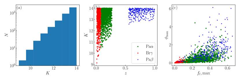
Figure 11: (a) The number of Type I AGNs with appropriate declinations for VLTI in each bin of $K$ band magnitudes. (b) The distribution of redshifts and $K$ band magnitude of objects with ${\rm Br}\gamma$, ${\rm Pa}\alpha$ or ${\rm Pa}\beta$ emission lines within the spectral coverage of GRAVITY. (c) The distribution of line intensities $f_{\ell{\rm,max}}$ and phase signal amplitudes $\phi_{\rm max}$ of objects in (b).

Appendix C Diffusive nested sampling

Nested sampling was proposed by Skilling (2004) to evaluate the evidence $Z$ of a model $M$:

$$Z\equiv P(\mathscr{D}|M)=\int P(\mathscr{D}|\bm{\Theta},M)P(\bm{\Theta}|M)\differential{\bm{\Theta}},$$ (C1)

where $\mathscr{D}$ and $\bm{\Theta}$ represent the data set and model parameters respectively, $P(\bm{\Theta}|M)$ is the prior probability distribution of parameters $\bm{\Theta}$ in model $M$ and $P(\mathscr{D}|\bm{\Theta},M)$ is the likelihood function.

Nested sampling starts with $n$ points $\bm{\Theta}_{i}$ sampled from prior $P(\bm{\Theta}|M)$. The likelihood of each point $L(\bm{\Theta}_{i})\equiv P(\mathscr{D}|\bm{\Theta}_{i},M)$ is evaluated. The minimum of likelihoods $L_{1}$ and corresponding particle is saved. Then this particle will be replaced by a new one drawn from the prior probability distribution but under a constraint $L(\bm{\Theta})>L_{1}$ via Markov chain Monte Carlo method. Again, the minimum of likelihoods of the living $n$ particles $L_{2}$ is saved and iteration continues. As nested likelihood levels $L_{1}<L_{2}<\cdots$ are created, particles move progressively towards higher likelihoods. The posterior distribution of $\bm{\Theta}$ can be obtained as a byproduct by recording positions and likelihoods of particles in the process.

There are several variants of nested samling, such as CosmoNest(Parkinson et al., 2011) and MultiNest(Feroz et al., 2009). Diffusive nested sampling (Brewer et al., 2011) is the one that makes improvements to the original method to overcome its drawbacks when sampling multimodal or highly correlated distributions. In the process of creating levels, particles at high levels can diffuse to lower levels. If a distribution has isolate islands with high likelihoods, particles in classic nested sampling may be stuck in one island and fail to explore other islands. However, particles in diffusive nested sampling can diffuse to lower levels where the distribution is sufficently broad without isolate islands so that particles can easily move over the whole parameter space.

Diffusive nested sampling peforms well to overcome high dimensions, multimodal distributions and phase changes. It has been successfully applied to fit the broad line region model to reverberation mapping and spectroastrometry data to measure the broad line region size, black hole mass, and distance to the quasar (e.g. Pancoast et al., 2014b; Li et al., 2018; Wang et al., 2020).

References

- Abbott et al. (2017a) Abbott, B. P., Abbott, R., Abbott, T. D., et al. 2017a, Phys. Rev. Lett., 119, 161101, doi: 10.1103/PhysRevLett.119.161101
- Abbott et al. (2017b) —. 2017b, ApJ, 848, L12, doi: 10.3847/2041-8213/aa91c9
- Abbott et al. (2017c) —. 2017c, Nature, 551, 85, doi: 10.1038/nature24471
- Bentz et al. (2021) Bentz, M. C., Street, R., Onken, C. A., & Valluri, M. 2021, ApJ, 906, 50, doi: 10.3847/1538-4357/abccd4
- Bentz et al. (2010) Bentz, M. C., Walsh, J. L., Barth, A. J., et al. 2010, ApJ, 716, 993, doi: 10.1088/0004-637X/716/2/993
- Bentz et al. (2013) Bentz, M. C., Denney, K. D., Grier, C. J., et al. 2013, ApJ, 767, 149, doi: 10.1088/0004-637X/767/2/149
- Blandford & McKee (1982) Blandford, R. D., & McKee, C. F. 1982, ApJ, 255, 419, doi: 10.1086/159843
- Blinov et al. (2019) Blinov, N., Kelly, K. J., Krnjaic, G., & McDermott, S. D. 2019, Phys. Rev. Lett., 123, 191102, doi: 10.1103/PhysRevLett.123.191102
- Brewer & Foreman-Mackey (2018) Brewer, B. J., & Foreman-Mackey, D. 2018, JOURNAL OF STATISTICAL SOFTWARE, 86, 1, doi: 10.18637/jss.v086.i07
- Brewer et al. (2011) Brewer, B. J., Pártay, L. B., & Csányi, G. 2011, Statistics and Computing, 21, 649, doi: 10.1007/s11222-010-9198-8
- Brotherton et al. (2020) Brotherton, M. S., Du, P., Xiao, M., et al. 2020, arXiv e-prints, arXiv:2011.05902. https://arxiv.org/abs/2011.05902
- Buen-Abad et al. (2015) Buen-Abad, M. A., Marques-Tavares, G., & Schmaltz, M. 2015, Phys. Rev. D, 92, 023531, doi: 10.1103/PhysRevD.92.023531
- Cai & Yang (2017) Cai, R.-G., & Yang, T. 2017, Phys. Rev. D, 95, 044024, doi: 10.1103/PhysRevD.95.044024
- Chen et al. (2018) Chen, H.-Y., Fishbach, M., & Holz, D. E. 2018, Nature, 562, 545, doi: 10.1038/s41586-018-0606-0
- Davis et al. (2019) Davis, T. M., Hinton, S. R., Howlett, C., & Calcino, J. 2019, MNRAS, 490, 2948, doi: 10.1093/mnras/stz2652
- Dexter et al. (2020) Dexter, J., Lutz, D., Shimizu, T. T., et al. 2020, arXiv e-prints, arXiv:2010.09735. https://arxiv.org/abs/2010.09735
- Di Valentino et al. (2017) Di Valentino, E., Melchiorri, A., & Mena, O. 2017, Phys. Rev. D, 96, 043503, doi: 10.1103/PhysRevD.96.043503
- Di Valentino et al. (2016) Di Valentino, E., Melchiorri, A., & Silk, J. 2016, Physics Letters B, 761, 242, doi: 10.1016/j.physletb.2016.08.043
- Du & Wang (2019) Du, P., & Wang, J.-M. 2019, ApJ, 886, 42, doi: 10.3847/1538-4357/ab4908
- Du et al. (2016) Du, P., Lu, K.-X., Hu, C., et al. 2016, ApJ, 820, 27, doi: 10.3847/0004-637X/820/1/27
- Du et al. (2018) Du, P., Zhang, Z.-X., Wang, K., et al. 2018, ApJ, 856, 6, doi: 10.3847/1538-4357/aaae6b
- Eisenhauer et al. (2008) Eisenhauer, F., Perrin, G., Brandner, W., et al. 2008, in Society of Photo-Optical Instrumentation Engineers (SPIE) Conference Series, Vol. 7013, Proc. SPIE, 70132A
- Feroz et al. (2009) Feroz, F., Hobson, M. P., & Bridges, M. 2009, MNRAS, 398, 1601, doi: 10.1111/j.1365-2966.2009.14548.x
- Fischer et al. (2013) Fischer, T. C., Crenshaw, D. M., Kraemer, S. B., & Schmitt, H. R. 2013, ApJS, 209, 1, doi: 10.1088/0067-0049/209/1/1
- Fonseca Alvarez et al. (2020) Fonseca Alvarez, G., Trump, J. R., Homayouni, Y., et al. 2020, ApJ, 899, 73, doi: 10.3847/1538-4357/aba001
- Foreman-Mackey (2016) Foreman-Mackey, D. 2016, The Journal of Open Source Software, 1, 24, doi: 10.21105/joss.00024
- Gravity Collaboration et al. (2017) Gravity Collaboration, Abuter, R., Accardo, M., et al. 2017, A&A, 602, A94, doi: 10.1051/0004-6361/201730838
- Gravity Collaboration et al. (2018) Gravity Collaboration, Sturm, E., Dexter, J., et al. 2018, Nature, 563, 657, doi: 10.1038/s41586-018-0731-9
- GRAVITY Collaboration et al. (2020) GRAVITY Collaboration, Amorim, A., Brandner, W., et al. 2020, arXiv e-prints, arXiv:2009.08463. https://arxiv.org/abs/2009.08463
- Grier et al. (2013) Grier, C. J., Peterson, B. M., Horne, K., et al. 2013, ApJ, 764, 47, doi: 10.1088/0004-637X/764/1/47
- Grier et al. (2017) Grier, C. J., Trump, J. R., Shen, Y., et al. 2017, ApJ, 851, 21, doi: 10.3847/1538-4357/aa98dc
- Hopkins et al. (2007) Hopkins, P. F., Richards, G. T., & Hernquist, L. 2007, ApJ, 654, 731, doi: 10.1086/509629
- Horne (1994) Horne, K. 1994, in Astronomical Society of the Pacific Conference Series, Vol. 69, Reverberation Mapping of the Broad-Line Region in Active Galactic Nuclei, ed. P. M. Gondhalekar, K. Horne, & B. M. Peterson, 23
- Hu (in press) Hu, C. in press, ApJ
- Huang & Wang (2016) Huang, Q.-G., & Wang, K. 2016, European Physical Journal C, 76, 506, doi: 10.1140/epjc/s10052-016-4352-x
- Hubble (1929) Hubble, E. 1929, Proceedings of the National Academy of Science, 15, 168, doi: 10.1073/pnas.15.3.168
- Kaspi et al. (2000) Kaspi, S., Smith, P. S., Netzer, H., et al. 2000, ApJ, 533, 631, doi: 10.1086/308704
- Kelly et al. (2009) Kelly, B. C., Bechtold, J., & Siemiginowska, A. 2009, ApJ, 698, 895, doi: 10.1088/0004-637X/698/1/895
- Ko & Tang (2016) Ko, P., & Tang, Y. 2016, Physics Letters B, 762, 462, doi: 10.1016/j.physletb.2016.10.001
- Kreisch et al. (2020) Kreisch, C. D., Cyr-Racine, F.-Y., & Doré, O. 2020, Phys. Rev. D, 101, 123505, doi: 10.1103/PhysRevD.101.123505
- Kun et al. (2015) Kun, E., Frey, S., Gabányi, K. É., et al. 2015, MNRAS, 454, 1290, doi: 10.1093/mnras/stv2049
- Landt et al. (2008) Landt, H., Bentz, M. C., Ward, M. J., et al. 2008, ApJS, 174, 282, doi: 10.1086/522373
- Li (2020) Li, Y.-R. 2020, LiyrAstroph/CDNest: CDNest: A diffusive nested sampling code in C, v0.2.0, Zenodo, doi: 10.5281/zenodo.3884449
- Li et al. (2013) Li, Y.-R., Wang, J.-M., Ho, L. C., Du, P., & Bai, J.-M. 2013, ApJ, 779, 110, doi: 10.1088/0004-637X/779/2/110
- Li et al. (2018) Li, Y.-R., Songsheng, Y.-Y., Qiu, J., et al. 2018, ApJ, 869, 137, doi: 10.3847/1538-4357/aaee6b
- Liu et al. (2019) Liu, H.-Y., Liu, W.-J., Dong, X.-B., et al. 2019, ApJS, 243, 21, doi: 10.3847/1538-4365/ab298b
- Lu et al. (2016) Lu, K.-X., Du, P., Hu, C., et al. 2016, ApJ, 827, 118, doi: 10.3847/0004-637X/827/2/118
- Lusso et al. (2012) Lusso, E., Comastri, A., Simmons, B. D., et al. 2012, MNRAS, 425, 623, doi: 10.1111/j.1365-2966.2012.21513.x
- Lynden-Bell (1969) Lynden-Bell, D. 1969, Nature, 223, 690, doi: 10.1038/223690a0
- Marconi et al. (2003) Marconi, A., Maiolino, R., & Petrov, R. G. 2003, Ap&SS, 286, 245, doi: 10.1023/A:1026100831792
- Pancoast et al. (2011) Pancoast, A., Brewer, B. J., & Treu, T. 2011, ApJ, 730, 139, doi: 10.1088/0004-637X/730/2/139
- Pancoast et al. (2014a) —. 2014a, MNRAS, 445, 3055, doi: 10.1093/mnras/stu1809
- Pancoast et al. (2014b) Pancoast, A., Brewer, B. J., Treu, T., et al. 2014b, MNRAS, 445, 3073, doi: 10.1093/mnras/stu1419
- Parkinson et al. (2011) Parkinson, D., Mukherjee, P., & Liddle, A. 2011, CosmoNest: Cosmological Nested Sampling. http://ascl.net/1110.019
- Perlmutter et al. (1999) Perlmutter, S., Aldering, G., Goldhaber, G., et al. 1999, ApJ, 517, 565, doi: 10.1086/307221
- Peterson (1993) Peterson, B. M. 1993, PASP, 105, 247, doi: 10.1086/133140
- Peterson et al. (1998) Peterson, B. M., Wanders, I., Bertram, R., et al. 1998, ApJ, 501, 82, doi: 10.1086/305813
- Peterson et al. (2004) Peterson, B. M., Ferrarese, L., Gilbert, K. M., et al. 2004, ApJ, 613, 682, doi: 10.1086/423269
- Petrov (1989) Petrov, R. G. 1989, in NATO Advanced Science Institutes (ASI) Series C, Vol. 274, NATO Advanced Science Institutes (ASI) Series C, ed. D. M. Alloin & J. M. Mariotti, 249
- Petrov et al. (2001) Petrov, R. G., Malbet, F., Richichi, A., et al. 2001, Comptes Rendus Physique, 2, 67. https://arxiv.org/abs/astro-ph/0507398
- Planck Collaboration et al. (2018) Planck Collaboration, Aghanim, N., Akrami, Y., et al. 2018, arXiv e-prints, arXiv:1807.06209. https://arxiv.org/abs/1807.06209
- Raimundo et al. (2019) Raimundo, S. I., Pancoast, A., Vestergaard, M., Goad, M. R., & Barth, A. J. 2019, MNRAS, 489, 1899, doi: 10.1093/mnras/stz2243
- Raimundo et al. (2020) Raimundo, S. I., Vestergaard, M., Goad, M. R., et al. 2020, MNRAS, 493, 1227, doi: 10.1093/mnras/staa285
- Rakshit et al. (2015) Rakshit, S., Petrov, R. G., Meilland, A., & Hönig, S. F. 2015, MNRAS, 447, 2420, doi: 10.1093/mnras/stu2613
- Rameez & Sarkar (2019) Rameez, M., & Sarkar, S. 2019, arXiv e-prints, arXiv:1911.06456. https://arxiv.org/abs/1911.06456
- Rees (1984) Rees, M. J. 1984, ARA&A, 22, 471, doi: 10.1146/annurev.aa.22.090184.002351
- Refsdal (1964) Refsdal, S. 1964, MNRAS, 128, 307, doi: 10.1093/mnras/128.4.307
- Riess et al. (2019) Riess, A. G., Casertano, S., Yuan, W., Macri, L. M., & Scolnic, D. 2019, ApJ, 876, 85, doi: 10.3847/1538-4357/ab1422
- Riess et al. (1998) Riess, A. G., Filippenko, A. V., Challis, P., et al. 1998, AJ, 116, 1009, doi: 10.1086/300499
- Rose et al. (2020) Rose, B. M., Rubin, D., Strolger, L., & Garnavich, P. 2020, in American Astronomical Society Meeting Abstracts, American Astronomical Society Meeting Abstracts, 108.01
- Schutz (1986) Schutz, B. F. 1986, Nature, 323, 310, doi: 10.1038/323310a0
- Shaw et al. (2007) Shaw, J. R., Bridges, M., & Hobson, M. P. 2007, MNRAS, 378, 1365, doi: 10.1111/j.1365-2966.2007.11871.x
- Shen et al. (2016) Shen, Y., Horne, K., Grier, C. J., et al. 2016, ApJ, 818, 30, doi: 10.3847/0004-637X/818/1/30
- Skilling (2004) Skilling, J. 2004, in American Institute of Physics Conference Series, Vol. 735, Bayesian Inference and Maximum Entropy Methods in Science and Engineering: 24th International Workshop on Bayesian Inference and Maximum Entropy Methods in Science and Engineering, ed. R. Fischer, R. Preuss, & U. V. Toussaint, 395–405
- Skilling (2006) Skilling, J. 2006, Bayesian Analysis, 1, 833, doi: 10.1214/06-BA127
- Soares-Santos et al. (2017) Soares-Santos, M., Holz, D. E., Annis, J., et al. 2017, ApJ, 848, L16, doi: 10.3847/2041-8213/aa9059
- Songsheng et al. (2019a) Songsheng, Y.-Y., Wang, J.-M., & Li, Y.-R. 2019a, ApJ, 883, 184, doi: 10.3847/1538-4357/ab3c5e
- Songsheng et al. (2019b) Songsheng, Y.-Y., Wang, J.-M., Li, Y.-R., & Du, P. 2019b, ApJ, 881, 140, doi: 10.3847/1538-4357/ab2e00
- Suyu et al. (2017) Suyu, S. H., Bonvin, V., Courbin, F., et al. 2017, MNRAS, 468, 2590, doi: 10.1093/mnras/stx483
- Verde et al. (2019) Verde, L., Treu, T., & Riess, A. G. 2019, Nature Astronomy, 3, 891, doi: 10.1038/s41550-019-0902-0
- Wang et al. (2020) Wang, J.-M., Songsheng, Y.-Y., Li, Y.-R., Du, P., & Zhang, Z.-X. 2020, Nature Astronomy, 4, 517, doi: 10.1038/s41550-019-0979-5
- Williams et al. (2018) Williams, P. R., Pancoast, A., Treu, T., et al. 2018, ApJ, 866, 75, doi: 10.3847/1538-4357/aae086
- Wong et al. (2020) Wong, K. C., Suyu, S. H., Chen, G. C. F., et al. 2020, MNRAS, doi: 10.1093/mnras/stz3094
- Xiao et al. (2018) Xiao, M., Du, P., Horne, K., et al. 2018, ApJ, 864, 109, doi: 10.3847/1538-4357/aad5e1
- Zhang et al. (2019) Zhang, Z.-X., Du, P., Smith, P. S., et al. 2019, ApJ, 876, 49, doi: 10.3847/1538-4357/ab1099
- Zhao et al. (2017) Zhao, G.-B., Raveri, M., Pogosian, L., et al. 2017, Nature Astronomy, 1, 627, doi: 10.1038/s41550-017-0216-z
- Zu et al. (2013) Zu, Y., Kochanek, C. S., Kozłowski, S., & Udalski, A. 2013, ApJ, 765, 106, doi: 10.1088/0004-637X/765/2/106