Prism: A Rich Class of Parameterized Submodular Information Measures for Guided Subset Selection

Abstract

With ever-increasing dataset sizes, subset selection techniques are becoming increasingly important for a plethora of tasks. It is often necessary to guide the subset selection to achieve certain desiderata, which includes focusing or targeting certain data points, while avoiding others. Examples of such problems include: i) targeted learning, where the goal is to find subsets with rare classes or rare attributes on which the model is underperforming, and ii) guided summarization, where data (e.g., image collection, text, document or video) is summarized for quicker human consumption with specific additional user intent. Motivated by such applications, we present Prism, a rich class of PaRameterIzed Submodular information Measures. Through novel functions and their parameterizations, Prism offers a variety of modeling capabilities that enable a trade-off between desired qualities of a subset like diversity or representation and similarity/dissimilarity with a set of data points. We demonstrate how Prism can be applied to the two real-world problems mentioned above, which require guided subset selection. In doing so, we show that Prism interestingly generalizes some past work, therein reinforcing its broad utility. Through extensive experiments on diverse datasets, we demonstrate the superiority of Prism over the state-of-the-art in targeted learning and in guided image-collection summarization. Prism is available as a part of the Submodlib (https://github.com/decile-team/submodlib) and Trust (https://github.com/decile-team/trust) toolkits.

1 Introduction

Recent times have seen explosive growth in data across several modalities, including text, images, and videos. This has given rise to the need for finding techniques for selecting effective smaller data subsets with specific characteristics for a variety of down-stream tasks. Often, we would like to guide the data selection to either target or avoid a certain set of data slices. One application is, what we call, targeted learning, where the goal is to select data points similar to data slices on which the model is currently performing poorly. These slices are data points that either belong to rare classes or have common rare attributes (e.g., color, background, etc.). An example of such a scenario is shown in Fig. 1(a), where a self-driving car model struggles in detecting “cars in a dark background“ because of a lack of such images in the training set. The targeted learning problem is to augment the training dataset with more of such rare images, with an aim to improve model performance. Another example is detecting cancers in biomedical imaging datasets, where the number of cancerous images are often a small fraction of the non-cancerous images.

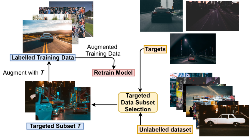
(a)

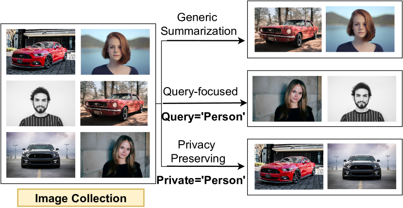
(b)

Figure 1: Applications of guided subset selection. (a) Targeted learning: improving a model’s performance on night images (target), which are under-represented in the training data. This is achieved by augmenting it with a subset matching the target. (b) Guided summarization: finding a summary similar to a query set or a summary dissimilar to a private set.

Another application comes from the summarization task, where an image collection, a video, or a text document is summarized for quicker human consumption by eliminating redundancy, while preserving the main content. While a number of applications require generic summarization (i.e., simply picking a representative and diverse subset of the massive dataset), it is often important to capture certain user intent in summarization. We call this guided summarization. Examples of guided summarization include: (i) query-focused summarization (Sharghi, Gong, and Shah 2016; Xiao et al. 2020), where a summary similar to a specific query is desired, and (ii) privacy-preserving summarization, where a summary dissimilar to a given private set of data points is desired (say, for privacy issues). See Fig. 1(b) for a pictorial illustration.

1.1 Our Contributions

Prism Framework: We define Prism through different instantiations and parameterizations of various submodular information measures (Sec. 2). These allow for modeling a spectrum of semantics required for guided subset selection, like relevance to a query set, irrelevance to a private set, and diversity among selected data points. We study the effect of parameter trade-off among these different semantics and present interesting insights.

Prism for Targeted Learning: We present a novel algorithm (Sec. 3.1, Algo. 1) to apply Prism for targeted learning, which aims to improve a model’s performance on rare slices of data. Specifically, we show that submodular information measures are very effective in finding the examples from the rare classes in a large unlabeled set (akin to finding a needle in a haystack). On several image classification tasks, Prism obtains $\approx$ 20-30% gain in accuracy of rare classes ($\approx$ 12% more than existing approaches) by just adding a few additional labeled points from the rare classes. Furthermore, we show that Prism is $20\times$ to $50\times$ more label-efficient compared to random sampling, and $2\times$ to $4\times$ more label-efficient compared to existing approaches (see Sec. 4.1). We also show that  Algo. 1 generalizes some existing approaches for data subset selection, reinforcing its utility (Sec. 3.3).

Prism for Guided Summarization. We propose a learning framework for guided summarization using Prism (Sec. 3.2). We show that Prism offers a unified treatment to the different flavors of guided summarization (query-focused and privacy-preserving) and generalizes some existing approaches to summarization, again reinforcing its utility. We show that it outperforms other existing approaches on a real-world image collections dataset (Sec. 4.2).

1.2 Related Work

Submodularity and Submodular Information Measures: Submodularity (Fujishige 2005) is a rich yet tractable subfield of non-linear combinatorial optimization (Krause and Golovin 2014).We provide novel formulations of the recently introduced class of submodular information measures (Gupta and Levin 2020; Iyer et al. 2021) for guided data subset selection.

Data Subset Selection, Coresets, and Active Learning: A number of papers have studied data subset selection in different applications and settings. Several recent papers have studied data subset selection for speeding up training. These include approaches involving submodularity (Wei, Iyer, and Bilmes 2015; Kaushal et al. 2019a), gradient coresets (Mirzasoleiman, Bilmes, and Leskovec 2020; Killamsetty et al. 2021) and bi-level based coresets (Killamsetty et al. 2020). Another application is active learning, where the goal is to select and label a subset of unlabeled data points to improve model performance (Settles 2009). Several recent approaches which combine notions of diversity and uncertainty have become popular (Wei, Iyer, and Bilmes 2015; Sener and Savarese 2018; Ash et al. 2020). One such state-of-the-art approach is Badge (Ash et al. 2020), which samples points that have diverse hypothesized gradients. Most of these paradigms have been studied in the setting of generic data subset selection, and are ineffective when it comes to guided subsets. Some recent works like Grad-match (Killamsetty et al. 2021) and Glister (Killamsetty et al. 2020) select subsets based on a held out validation set, which can be a rare slice of data. Similarly, (Kirchhoff and Bilmes 2014) compute a targeted subset of training data in the spirit of transductive learning for machine translation.

Summarization: A number of instances of summarization have been studied in the past, including image collection summarization (Celis and Keswani 2020; Ozkose et al. 2019; Singh, Virmani, and Subramanyam 2019; Tschiatschek et al. 2014), text/document summarization (Lin and Bilmes 2012; Chali, Tanvee, and Nayeem 2017; Yao, Wan, and Xiao 2017), and video summarization (Kaushal et al. 2019c, b; Gygli, Grabner, and Gool 2015; Ji et al. 2019). While most of these works have focused on generic summarization, some have also studied query-focused video summarization (Sharghi, Gong, and Shah 2016; Sharghi, Laurel, and Gong 2017; Vasudevan et al. 2017; Xiao et al. 2020; Jiang and Han 2019), and query-focused document summarization (Lin and Bilmes 2011; Li, Li, and Li 2012). To the best of our knowledge, Prism is the first attempt to offer a unified treatment to the different flavors of summarization.

2 The Prism Framework

2.1 Preliminaries

Submodular functions: Let $\mathcal{V}=\{1,2,3,...,n\}$ denote the ground-set and $f$ denote a set function $f:2^{\mathcal{V}}\xrightarrow{}\Re$. The function $f$ is submodular if it satisfies the diminishing marginal returns property; namely $f(j|\mathcal{X})\geq f(j|\mathcal{Y}),\forall\mathcal{X}\subseteq\mathcal{Y}\subseteq\mathcal{V},j\notin\mathcal{Y}$ (Fujishige 2005). Submodularity (along with monotonicity) ensures that a greedy algorithm achieves a $1-1/e$ approximation when $f$ is maximized (Nemhauser, Wolsey, and Fisher 1978).
Submodular Conditional Gain (CG): Given sets $\mathcal{A},\mathcal{P}\subseteq\mathcal{V}$, the CG, $f(\mathcal{A}|\mathcal{P})$, is the gain in function value by adding $\mathcal{A}$ to $\mathcal{P}$. Thus $f(\mathcal{A}|\mathcal{P})=f(\mathcal{A}\cup\mathcal{P})-f(\mathcal{P})$. Intuitively, $f(\mathcal{A}|\mathcal{P})$ measures how different $\mathcal{A}$ is from $\mathcal{P}$, where $\mathcal{P}$ is the conditioning set or the private set.
Submodular Mutual Information (MI): Given sets $\mathcal{A},\mathcal{Q}\subseteq\mathcal{V}$, the MI (Gupta and Levin 2020; Iyer et al. 2021) is defined as $I_{f}(\mathcal{A};\mathcal{Q})=f(\mathcal{A})+f(\mathcal{Q})-f(\mathcal{A}\cup\mathcal{Q})$. Intuitively, this measures the similarity between $\mathcal{Q}$ and $\mathcal{A}$ where $\mathcal{Q}$ is the query set.
Submodular Conditional Mutual Information (CMI): CMI is defined using CG and MI as $I_{f}(\mathcal{A};\mathcal{Q}|\mathcal{P})=f(\mathcal{A}\cup\mathcal{P})+f(\mathcal{Q}\cup\mathcal{P})-f(\mathcal{A}\cup\mathcal{Q}\cup\mathcal{P})-f(\mathcal{P})$. Intuitively, CMI jointly models the mutual similarity between $\mathcal{A}$ and $\mathcal{Q}$ and their collective dissimilarity from $\mathcal{P}$.

Properties: CG, MI, and CMI are non-negative and monotone in one argument with the other fixed (Gupta and Levin 2020; Iyer et al. 2021). CMI and MI are not necessarily submodular in one argument (with the others fixed) (Iyer et al. 2021). However, several of the instantiations we define below turn out to be submodular. With this background, we present our unique and novel formulations, leading to Prism.

2.2 Guidance from an Auxiliary Set

We formulate the above submodular information measures to handle the case when the guidance can come from an auxiliary set $\mathcal{V}^{\prime}$ different from the ground set $\mathcal{V}$ – a requirement common in several guided subset selection tasks. Let $\Omega=\mathcal{V}\cup\mathcal{V}^{\prime}$. We define a set function $f:2^{\Omega}\rightarrow\Re$. Although $f$ is defined on $\Omega$, the discrete optimization problem will only be defined on subsets $\mathcal{A}\subseteq\mathcal{V}$. To find an optimal subset (i) given a query set $\mathcal{Q}\subseteq\mathcal{V}^{\prime}$, we can define $g_{\mathcal{Q}}(\mathcal{A})=I_{f}(\mathcal{A};\mathcal{Q})$, $\mathcal{A}\subseteq\mathcal{V}$ and maximize the same; (ii) given a private set $\mathcal{P}\subseteq\mathcal{V}^{\prime}$, we can define $h_{\mathcal{P}}(\mathcal{A})=f(\mathcal{A}|\mathcal{P})$, $\mathcal{A}\subseteq\mathcal{V}$, as the function to be maximized.

2.3 Restricted Submodularity to Enable a Richer Class of MI and CG Functions

While submodular functions are expressive, many natural choices are not submodular everywhere. We do not need $f$ to be submodular everywhere on $\Omega$, since the sets we are optimizing on, are subsets of $\mathcal{V}$. Instead of requiring the submodular inequality to hold for all pairs of sets $(\mathcal{X},\mathcal{Y})\in 2^{\Omega}\times 2^{\Omega}$, we can consider only subsets of this power set pivoting on $\mathcal{V}\subseteq\Omega$. In particular, define a subset $\mathcal{C}\subseteq 2^{\Omega}$. Then restricted submodularity on $\mathcal{C}$ satisfies $f(\mathcal{X})+f(\mathcal{Y})\geq f(\mathcal{X}\cup\mathcal{Y})+f(\mathcal{X}\cap\mathcal{Y}),\forall(\mathcal{X},\mathcal{Y})\in\mathcal{C}$. Instances of restricted submodularity in the form of intersecting and crossing submodular functions have been considered in the past (Fujishige 2005). We consider the following form of restricted submodularity. Given sets $\mathcal{V}$ and $\mathcal{V}^{\prime}$ as above, define $\mathcal{C}(\mathcal{V},\mathcal{V}^{\prime})\subseteq 2^{\Omega}$ to be such that the sets $(\mathcal{X},\mathcal{Y})\in\mathcal{C}(\mathcal{V},\mathcal{V}^{\prime})$ satisfy either of the following conditions: i) $\mathcal{X}\subseteq\mathcal{V}$ or $\mathcal{X}\subseteq\mathcal{V}^{\prime}$ and $\mathcal{Y}$ is any set, or ii) $\mathcal{X}$ is any set and $\mathcal{Y}\subseteq\mathcal{V}$ or $\mathcal{Y}\subseteq\mathcal{V}^{\prime}$. We call the MI of a restricted submodular function as Generalized Mutual Information function (GMI). We use this notion of GMI to define Concave Over Modular (COM). The GMI function is non-negative and monotone (see Appendix B.1).

2.4 Instantiations & Parameterizations in Prism

In this section, we discuss the expressions for different instantiations of the above measures using different functions. We refer to them as •MI or •CG or •CMI where • is the submodular function using which the respective MI, CG or CMI measure is instantiated. While different submodular functions naturally model different characteristics such as representation, coverage, etc. (Kaushal et al. 2019c, b), the instantiations presented here additionally model similarity and dissimilarity to query and private sets respectively. These instantiations have parameters $\lambda,\eta$ and/or $\nu$, that govern the interplay among different characteristics. In several instantiations, we invoke a similarity matrix $S$ where $S_{ij}$ measures the similarity between elements $i$ and $j$ of sets that will be correspondingly specified. The rich class of functions in Prism thus helps model a broad spectrum of semantics. The mathematical expressions for each function are summarized in Tab. 1. Below, we provide further notations and intuitions for using these functions.

Table 1: Instantiations of Prism. Note that the functions formulate similarity with query set $Q$ and dissimilarity with private set $P$ which are the building blocks for targeted data subset selection.

(a) Instantiations of MI functions

MI	$I_{f}(\mathcal{A};\mathcal{Q})$
Flvmi	$\sum\limits_{i\in\mathcal{V}}\min(\max\limits_{j\in\mathcal{A}}S_{ij},\eta\max\limits_{j\in\mathcal{Q}}S_{ij})$
Flqmi	$\sum\limits_{i\in\mathcal{Q}}\max\limits_{j\in\mathcal{A}}S_{ij}+$ $\eta\sum\limits_{i\in\mathcal{A}}\max\limits_{j\in\mathcal{Q}}S_{ij}$
Gcmi	$2\lambda\sum\limits_{i\in\mathcal{A}}\sum\limits_{j\in\mathcal{Q}}S_{ij}$
Logdetmi	$\log\det(S_{\mathcal{A}})-\log\det(S_{\mathcal{A}}-\eta^{2}S_{\mathcal{A},\mathcal{Q}}S_{\mathcal{Q}}^{-1}S_{\mathcal{A},\mathcal{Q}}^{T})$
COM	$\eta\sum_{i\in\mathcal{A}}\psi(\sum_{j\in\mathcal{Q}}S_{ij})+\sum_{j\in\mathcal{Q}}\psi(\sum_{i\in\mathcal{A}}S_{ij})$

(b) Instantiations of CG and CMI functions

CG	$f(\mathcal{A}|\mathcal{P})$
Flcg	$\sum\limits_{i\in\mathcal{V}}\max(\max\limits_{j\in\mathcal{A}}S_{ij}-$ $\max\limits_{j\in\mathcal{P}}S_{ij},0)$
Logdetcg	$\log\det(S_{\mathcal{A}}-\nu^{2}S_{\mathcal{A},\mathcal{P}}S_{\mathcal{P}}^{-1}S_{\mathcal{A},\mathcal{P}}^{T})$
Gccg	$f(\mathcal{A})-2\lambda\nu\sum\limits_{i\in\mathcal{A},j\in\mathcal{P}}S_{ij}$

CMI	$I_{f}(\mathcal{A};\mathcal{Q}|\mathcal{P})$
Flcmi	$\sum\limits_{i\in\mathcal{V}}\max(\min(\max\limits_{j\in\mathcal{A}}S_{ij},$ $\max\limits_{j\in\mathcal{Q}}S_{ij})$ $-\max\limits_{j\in\mathcal{P}}S_{ij},0)$
Logdetcmi	$\log\frac{\det(I-S_{\mathcal{P}}^{-1}S_{\mathcal{P},\mathcal{Q}}S_{\mathcal{Q}}^{-1}S_{\mathcal{P},\mathcal{Q}}^{T})}{\det(I-S_{\mathcal{A}\cup\mathcal{P}}^{-1}S_{\mathcal{A}\cup\mathcal{P},Q}S_{\mathcal{Q}}^{-1}S_{\mathcal{A}\cup\mathcal{P},Q}^{T})}$

Log Determinant (LogDet): Let $S_{\mathcal{A},\mathcal{Q}}$ be the cross-similarity matrix between the items in sets $\mathcal{A}$ and $\mathcal{Q}$. We construct a similarity matrix $S^{\eta,\nu}$ (on a base matrix $S$) in such a way that the cross-similarity between $\mathcal{A}$ and $\mathcal{Q}$ is multiplied by $\eta$ (i.e., $S^{\eta,\nu}_{\mathcal{A},\mathcal{Q}}=\eta S_{\mathcal{A},\mathcal{Q}}$) to control the trade-off between query-relevance and diversity. Similarly, the cross-similarity between $\mathcal{A}$ and $\mathcal{P}$ by $\nu$ (i.e., $S^{\eta,\nu}_{\mathcal{A},\mathcal{P}}=\nu S_{\mathcal{A},\mathcal{P}}$) to control the strictness of privacy constraints. Higher values of $\nu$ ensure stricter privacy constraints, such as in the context of privacy-preserving summarization, by tightening the extent of dissimilarity of the subset from the private set. Given the standard form of LogDet as $f(\mathcal{A})=\log\det(S^{\eta,\nu}_{\mathcal{A}})$, we provide the Prism expressions in Tab. 1. For simplicity of notation, CMI is presented with $\nu=\eta=1$. We defer the derivation and the general expression for CMI to the Appendix C.1.

Facility Location (FL): We introduce two variants of the MI functions for the FL function which is defined as: $f(\mathcal{A})=\sum_{i\in\Omega}\max_{j\in\mathcal{A}}S_{ij}$. The first variant is defined over $\mathcal{V}$ (FLVMI)  (Iyer et al. 2021), in Tab. 1(a). We derive another variant defined over $\mathcal{Q}$ (FLQMI) which considers only cross-similarities between data points and the target. This MI expression has interesting characteristics different from those of Flvmi. In particular, whereas Flvmi gets saturated (i.e., once the query is satisfied, there is no gain in picking another query-relevant data point), Flqmi just models the pairwise similarities of target to data points and vice versa. Moreover, Flqmi only requires a $\mathcal{Q}\times\mathcal{V}$ kernel, which makes it very efficient to optimize. We provide the expressions in Tab. 1 and defer the derivations to Appendix C.2. We multiply the similarity kernel $S$ used in MI and CG expressions of FL by $\eta$ and $\nu$ as done in the case of LogDet.

Concave Over Modular (COM): The notion of GMI functions (Sec. 2.3) allows us to characterize a rich class of concave over modular functions as GMI functions. Define a set function $f_{\eta}(\mathcal{A})$ as: $f_{\eta}(\mathcal{A})=\eta\sum_{i\in\mathcal{V}^{\prime}}\max(\psi(\sum_{j\in\mathcal{A}\cap\mathcal{V}}S_{ij}),\psi(\sqrt{n}\sum_{j\in\mathcal{A}\cap\mathcal{V}^{\prime}}S_{ij}))+\sum_{i\in\mathcal{V}}\max(\psi(\sum_{j\in\mathcal{A}\cap\mathcal{V}^{\prime}}S_{ij}),\psi(\sqrt{n}\sum_{j\in\mathcal{A}\cap\mathcal{V}}S_{ij}))$, where $\psi$ is a concave function and $f_{\eta}(\mathcal{A})$ is restricted submodular. We state the expression for its GMI function in Tab. 1(a) and provide the derivation in Appendix B.2.

Graph Cut (GC): The GC function is defined as $f(\mathcal{A})=\sum\limits_{i\in\mathcal{A},j\in\mathcal{V}}S_{ij}-\lambda\sum\limits_{i,j\in\mathcal{A}}S_{ij}$. The parameter $\lambda$ captures the trade-off between diversity and representativeness. The Prism expressions of GC are presented in Tab. 1. Note that the CMI expression for GC is not useful as it does not involve the private set and is exactly the same as the MI version (proof in Appendix C.3). Like in the LogDet case, we introduce an additional parameter $\nu$ in Gccg to control the strictness of privacy constraints. Again, this is easily modeled in the GC objective by multiplying the cross-similarity between data points and the private instances by $\nu$.

Computational Complexity: In terms of compute complexity, Gcmi and Flqmi are linear in $|\mathcal{V}|$ (since $\mathcal{Q}$ is typically small). However, Flvmi and Logdetmi are quadratic in the size of the unlabeled set due to requiring the kernel. Hence, for massive datasets, Gcmi and Flqmi are preferable (more details in Appendix D). We also discuss (in Appendix D) a partitioning based approach where we divide the datasets into smaller partitions and run the $\mathcal{V}\times\mathcal{V}$ kernel based functions (Flvmi and Logdetmi) on the individual partitions, thereby making them more scalable.

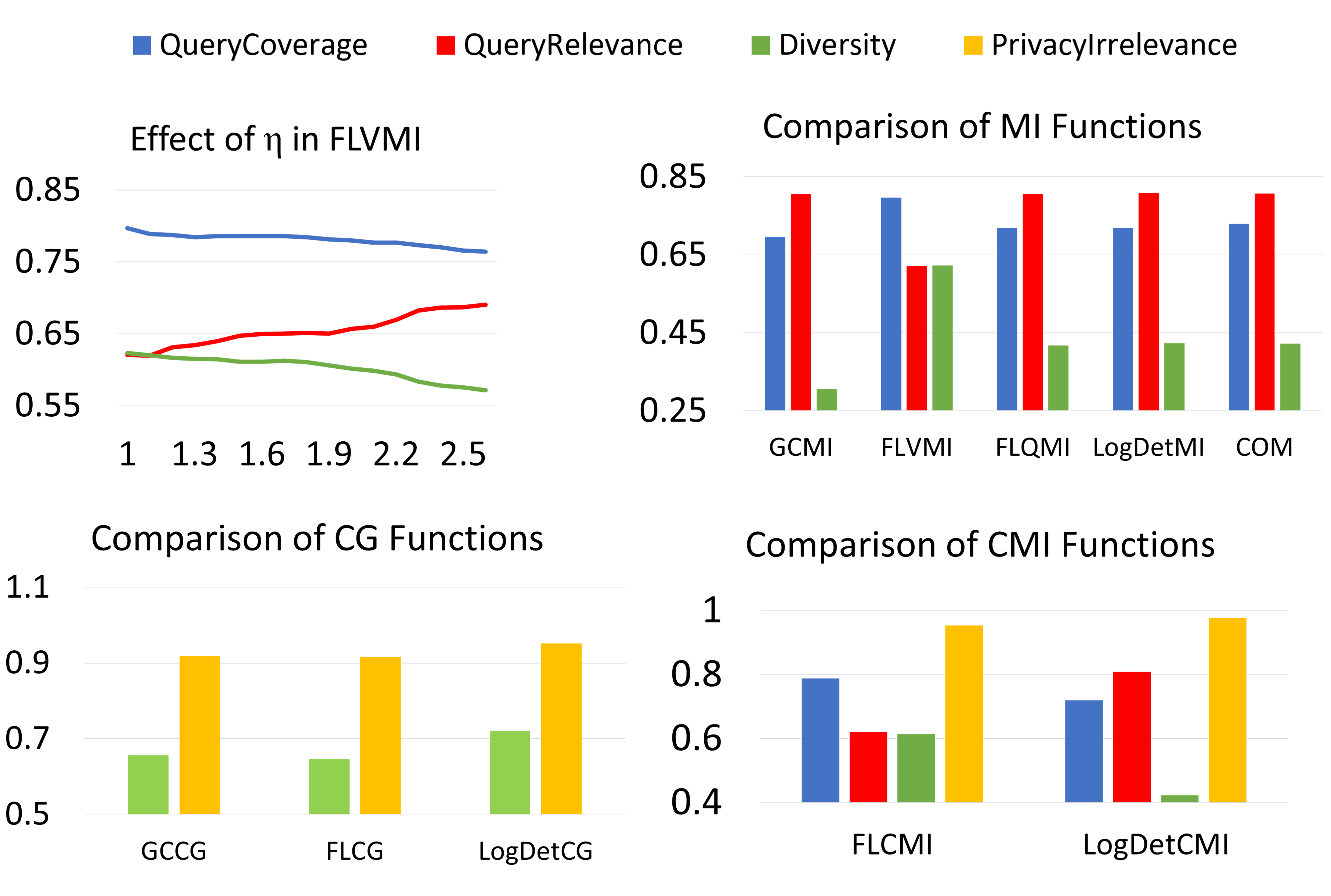
Figure 2: Behavior of different functions in Prism and effect of parameters. All plots share the legend.

2.5 Modeling Semantics of Prism

To empirically verify the intuitive understanding of the expressions, we maximize the different functions in Prism individually on a synthetically created dataset with different parameters, and study the characteristics of the subsets qualitatively and quantitatively. For evaluation, we define query-coverage to be the fraction of queries covered by the subset, query-relevance to be the fraction of the subset pertaining to the queries, diversity to be the measure of how diverse are the points within the selected subset, and privacy-irrelevance to be the fraction of the subset not matching the private set. We present representative results in Fig. 2 and defer detailed results to Appendix E. For MI functions, we verify that increasing $\eta$ tends to increase query-relevance while reducing query-coverage and diversity (top-left, Fig. 2). Also, while Gcmi lies at one end of the spectrum favoring query-relevance, Flvmi lies at the other end favoring diversity and query coverage. Flqmi, Logdetmi and COM lie somewhere in between (top-right, Fig. 2). As expected, increasing $\nu$ increases privacy-irrelevance for CG functions. We also observe that Logdetcg outperforms Flcg and Gccg both in terms of diversity and privacy-irrelevance (bottom-left, Fig. 2). For CMI functions, we see that Flcmi tends to favor query-coverage and diversity in contrast to query-relevance and privacy-irrelevance, while Logdetcmi favors query-relevance and privacy-irrelevance over query-coverage and diversity (bottom-right, Fig. 2).

3 Prism for Guided Subset Selection

In this section, we discuss the use of Prism for guided data subset selection and illustrate its utility for targeted learning and guided summarization.

3.1 Targeted Learning

We first apply Prism to targeted learning, where the goal is to improve a model’s accuracy on some target classes at a given additional labeling cost and without compromising on the overall accuracy (see Fig. 1(a)). Let $\mathcal{E}$ be an initial training set of labeled instances, ${\mathcal{T}}$ be the target set of examples on which the user desires good performance, $\mathcal{P}$ be the private set of examples that the user wants to avoid, and $\mathcal{U}$ be a large unlabeled dataset. We maximize a CMI function $I_{f}(\mathcal{A};{\mathcal{T}}|\mathcal{P})$ towards computing an optimal subset $\hat{\mathcal{A}}\subseteq\mathcal{U}$ of size $k$ similar to ${\mathcal{T}}$ and dissimilar to $\mathcal{P}$. Note that when $\mathcal{P}=\emptyset$, CMI is equivalent to MI. We then augment $\mathcal{E}$ with labeled $\hat{\mathcal{A}}$ and re-train the model. Through the aforementioned (Sec. 2), the diverse class of MI functions in Prism offers a natural and effective approach for targeted subset selection by using the query set $\mathcal{Q}$ as the target set ${\mathcal{T}}$. The approach is outlined in Algo. 1. Similar to (Ash et al. 2020; Killamsetty et al. 2020, 2021; Mirzasoleiman, Bilmes, and Leskovec 2020), we use last-layer gradients of the model to represent the data points and use them to compute the similarity kernel $S$. Specifically, we define pairwise similarities $S_{ij}=\langle\nabla_{\theta}\mathcal{L}_{i}(\theta),\nabla_{\theta}\mathcal{L}_{j}(\theta)\rangle$, where $\mathcal{L}_{i}(\theta)=\mathcal{L}(x_{i},y_{i},\theta)$ is the loss on the $i$th data point and $\theta$ denotes model parameters. Note that the target need not correspond to class(es) but could be any attribute of data that the user is interested in. For instance, the target could be mining images with people at night (here night is an attribute).

0:  $\mathcal{E}$: initial labeled set, $\mathcal{U}$: large unlabeled set, ${\mathcal{T}}$: a target subset/slice, $\mathcal{P}$: a set to be avoided, $k$: selection budget, $\mathcal{L}$: loss function

1:  Train model with loss $\mathcal{L}$ on labeled set $\mathcal{E}$ to obtain model parameters $\theta_{\mathcal{E}}$ {Obtain initial accuracy}

2:  Compute the gradients $\{\nabla_{\theta_{\mathcal{E}}}\mathcal{L}(x_{i},y_{i}),i\in\mathcal{U}\}$ (using hypothesized labels) and $\{\nabla_{\theta_{\mathcal{E}}}\mathcal{L}(x_{i},y_{i}),i\in{\mathcal{T}}\}$ {Obtain vectors for computing kernel in Step 3}

3:  Compute the similarity kernels $S$ and define a CMI function $I_{f}(\mathcal{A};{\mathcal{T}}|\mathcal{P})$ {Instantiate Functions}

4:  $\hat{\mathcal{A}}\leftarrow\max_{\mathcal{A}\subseteq\mathcal{U},|\mathcal{A}|\leq k}(I_{f}(\mathcal{A};{\mathcal{T}}|\mathcal{P})$ {Obtain the subset optimally matching the target}

5:  Obtain the labels of the elements in $\hat{\mathcal{A}}$ as $L(\hat{\mathcal{A}})$ {Procure labels on the selected subset}

6:  Train a model on the combined labeled set $\mathcal{E}\cup L(\hat{\mathcal{A}})$ {Augment training data}

Algorithm 1 Application of Prism for Targeted Learning

3.2 Guided Summarization

Next, we apply Prism for guided summarization. In this task, we are given a set $\mathcal{V}$ of data points (images, sentences of a document, or frames/shots of a video), and the goal is to find a summary $\mathcal{A}\subseteq\mathcal{V}$ with certain desired characteristics. In query-focused summarization, we find a summary that is semantically similar to the query set, while in privacy-preserving summarization, the obtained summary should not contain data points that are similar to the private set.

Prism’s Unified Framework for Guided Summarization: Given sets $\mathcal{Q}$ and $\mathcal{P}$, and a submodular function $f$, consider the following master optimization problem involving CMI: $\max_{\mathcal{A}:|\mathcal{A}|\leq k}I_{f}(\mathcal{A};\mathcal{Q}|\mathcal{P})$. We discuss how the different flavors of summarization can be seen as special cases of this master optimization problem. Setting $\mathcal{Q}\leftarrow\mathcal{V}$ and $\mathcal{P}\leftarrow\emptyset$ yields generic summarization. Similarly, setting $\mathcal{Q}\leftarrow\mathcal{Q}$ and $\mathcal{P}\leftarrow\emptyset$ yields query-focused summarization with a query-set $\mathcal{Q}$. Setting $\mathcal{Q}\leftarrow\mathcal{V}$ and $\mathcal{P}\leftarrow\mathcal{P}$ gives privacy-preserving summarization. This framework allows us to address yet another flavor: joint query-focused and privacy preserving summarization where we set $\mathcal{Q}\leftarrow\mathcal{Q}$ and $\mathcal{P}\leftarrow\mathcal{P}$.

Parameter Learning in Prism for Guided Summarization: As discussed in Sec. 2, different instantiations of Prism along with their parameters offer a wide spectrum of modeling characteristics. Hence, when used individually, each imparts certain characteristics to the summaries. For summarization, we thus propose learning a mixture model supervised by summaries generated by humans. We learn a mixture of Prism functions (Lin and Bilmes 2012; Kaushal et al. 2019c, b; Tschiatschek et al. 2014) where the weights and the internal parameters $\lambda,\nu,\eta$ of the functions are jointly learned. We denote our parameter vector by $\Theta=(w,\eta,\lambda,\nu)$, and our Prism mixture model by $F(\Theta)=\sum_{i}w_{i}f_{i}(\mathcal{A},\gamma,\eta,\nu)$, with each $f_{i}$ being either one of the functions in Prism or one of pure diversity and representation functions such as Disparity-Sum and FL. Then, given $N$ training examples, $(\mathcal{V}^{(n)},\mathcal{Y}^{(n)})_{n=1}^{N}$ we apply gradient descent to learn the parameters $\Theta$ by optimizing the following large-margin formulation: $\min\limits_{\Theta\geq 0}\frac{1}{N}\sum_{n=1}^{N}\mathcal{L}_{n}(\Theta)+\frac{\lambda}{2}||\Theta||^{2}$, where $\mathcal{L}_{n}(\Theta)$ is the generalized hinge loss associated with training example $n$: $\mathcal{L}_{n}(\Theta)=\max\limits_{\mathcal{Y}\subset\mathcal{V}^{(n)},|\mathcal{Y}|\leq k}(F(\mathcal{Y},x^{(n)},\Theta)+l_{n}(\mathcal{Y}))-F(\mathcal{Y}^{(n)},x^{(n)},\Theta)$. Here, $\mathcal{Y}^{(n)}$ is a human summary for the $n^{th}$ ground set $\mathcal{V}^{(n)}$ (video, image collection, or text document), with corresponding features $x^{(n)}$. The specific objective functions and gradient computations in case of query-focused, privacy-preserving, and joint query-focused and privacy-preserving summarizations are presented in Appendix F. For generic summarization, we add the standard submodular functions modeling representation, diversity, coverage, etc. in the mixture. For query-focused summarization and privacy-preserving summarization, we instead use the MI and CG versions of the functions respectively as defined above. Once the parameters are learned, we instantiate the mixture model with the parameters and maximize it to get the desired summaries.

3.3 Connections to Past Work

Prism generalizes past work in both targeted learning and guided summarization. We summarize the connections below; for more details, see Appendix G.

Targeted Learning: A number of approaches like Glister (Killamsetty et al. 2020) and Grad-Match (Killamsetty et al. 2021) can be considered with a validation set, and hence used in the targeted setting. Similarly, Craig (Mirzasoleiman, Bilmes, and Leskovec 2020) can be extended to consider a validation set. In Appendix G.1, we show that Algo. 1 in fact generalizes Craig (using Flqmi), Glister (using Com), and Grad-Match (using Gcmi + Diversity).

Guided Summarization: A number of past works for summarization have inadvertently used instances of Prism. The query-DPP considered in (Sharghi, Gong, and Shah 2016; Sharghi, Laurel, and Gong 2017) is a special case of Logdetmi. Similarly, the graph-cut based query-relevance term in (Vasudevan et al. 2017; Lin 2012), and in  (Li, Li, and Li 2012) is actually Gcmi. Furthermore, the joint diversity and query-relevance term in (Lin and Bilmes 2011) is an instance of COM (with the square-root as the concave function, see Appendix G.2).

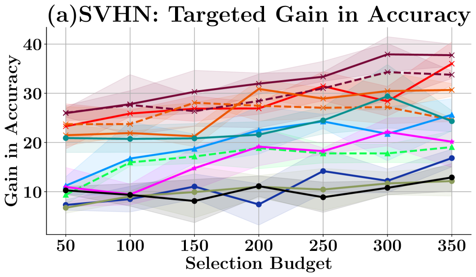
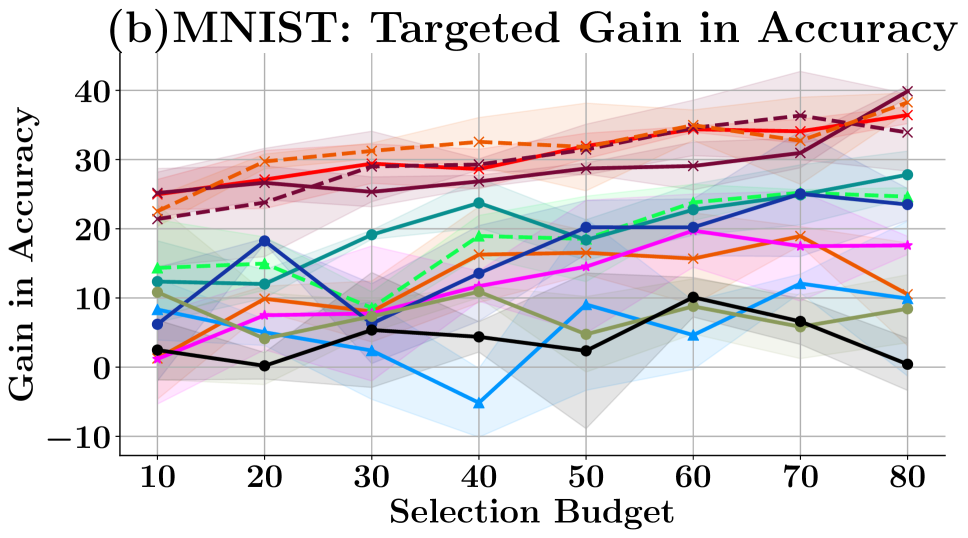
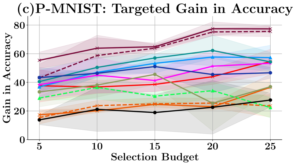
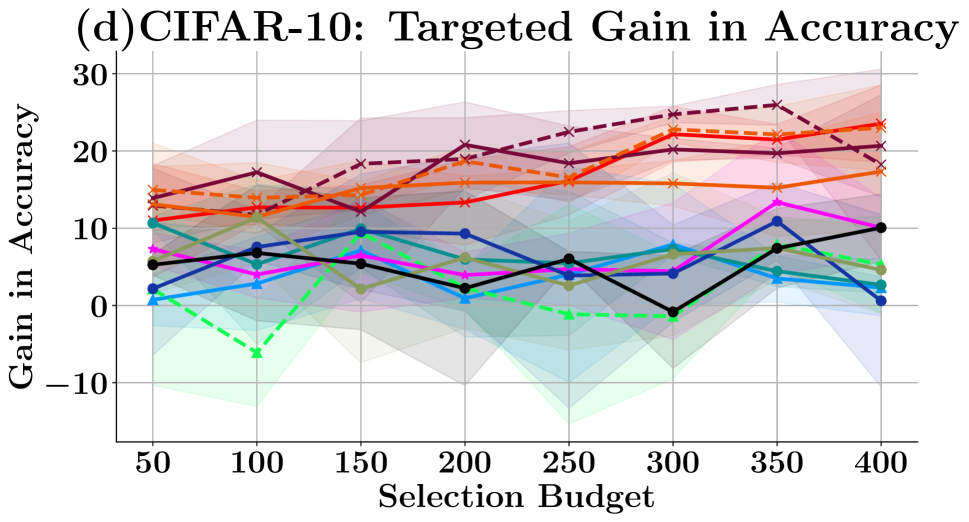
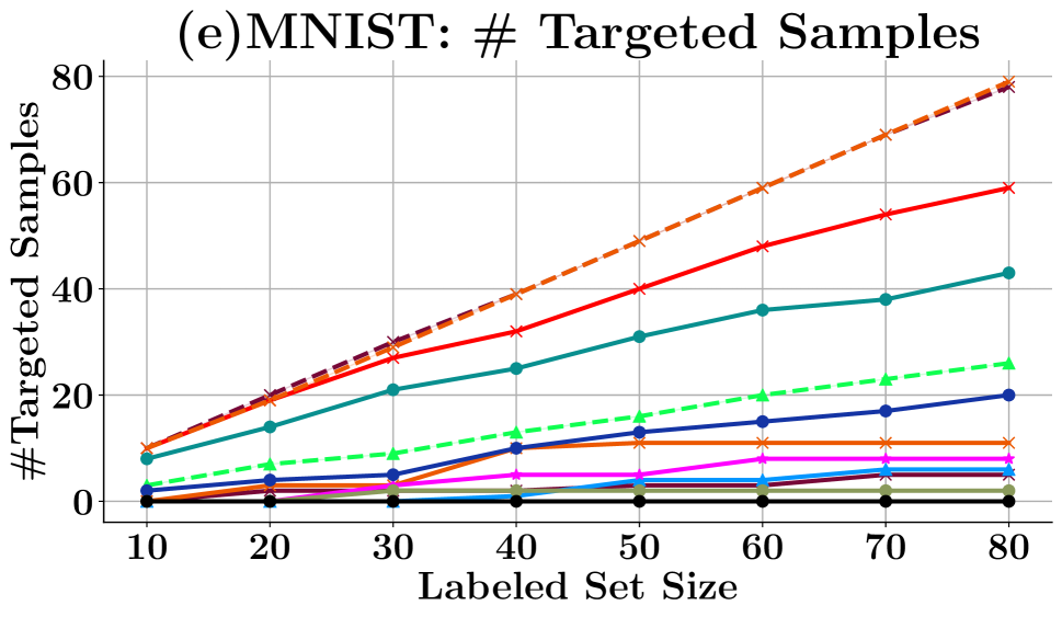
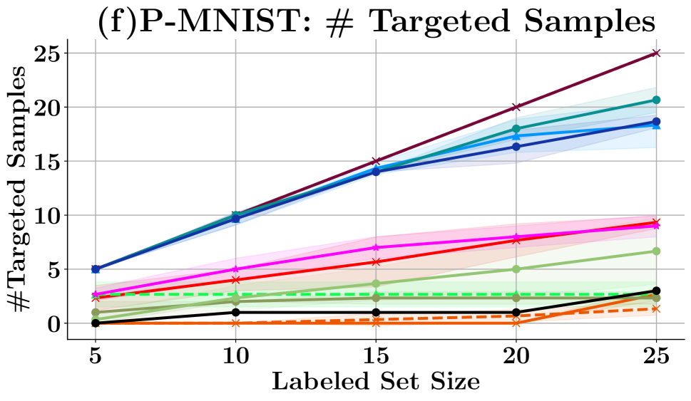
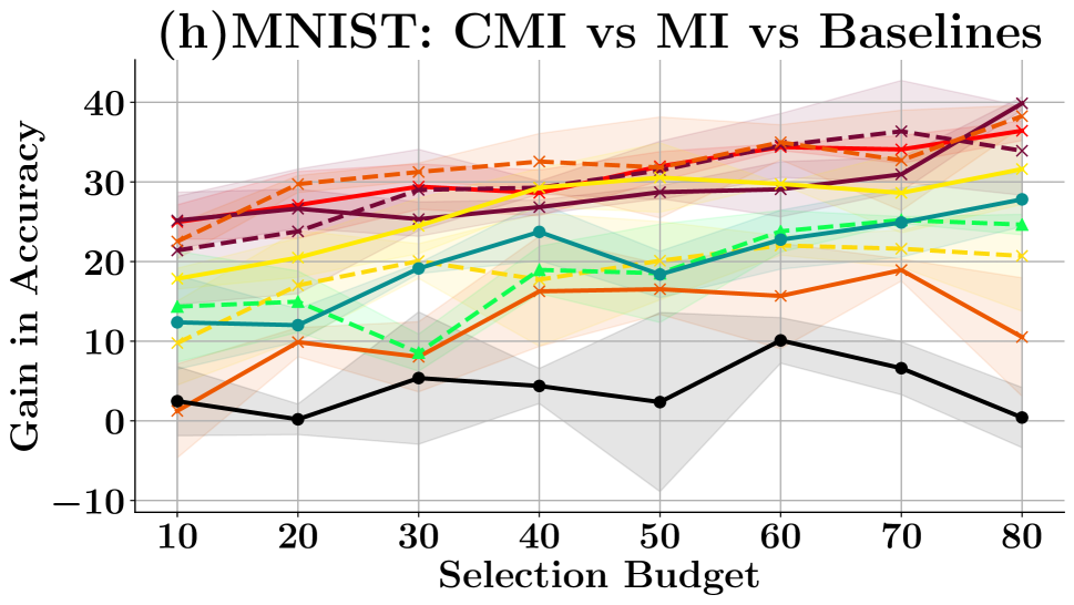
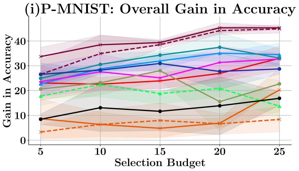
Figure 3: Targeted learning with Prism on SVHN, MNIST, P-MNIST (Pneumonia-MNIST) and CIFAR-10. Plots (a-d) compare average gain in accuracy on targeted classes. Plots (e-f) compare the number of data points selected from the targeted classes. Plots (g-h) show an ablation study to compare the performance of MI and CMI functions. Plot (i) shows the overall gain in accuracy on P-MNIST. The MI and CMI functions (specifically Flqmi and Flvmi) obtain larger gains in targeted (plots a-d) and overall accuracy (plot i) than other baselines by selecting larger and more diverse examples from targeted classes (plots e-f).

4 Experiments and Results

4.1 Targeted Learning

In this section, we demonstrate the effectiveness of Prism for targeted learning on the CIFAR-10 (Krizhevsky, Hinton et al. 2009), MNIST (LeCun et al. 1998), SVHN (Netzer et al. 2011), and P-MNIST (Pneumonia-MNIST) (Yang, Shi, and Ni 2021; Kermany et al. 2018) image classification datasets.

Custom dataset: To simulate a real-world setting, we randomly select some target classes and split the train set into labeled, target, and an unlabeled set such that (i) the labeled set has class imbalance and poorly represents the target classes, (ii) the target set has a small number of data points from the target classes, and (iii) the unlabeled set is a large set whose labels we do not use (resembling a large pool of unlabeled data in real-world scenarios). For CMI functions, we additionally use a private set, which has a small number of data points from the non-target classes. The performance is measured on the standard test set from the respective datasets. Let the set $\mathcal{C}$ consist of data points from the target classes and the set $\mathcal{D}$ consist of data points from the non-target classes. We create an initial labeled set $\mathcal{E}$, such that $|\mathcal{D}_{\mathcal{E}}|=\rho|\mathcal{C}_{\mathcal{E}}|$ and an unlabeled set which follows the same distribution $|\mathcal{D}_{\mathcal{U}}|=\rho|\mathcal{C}_{\mathcal{U}}|$, where $\rho$ is the imbalance ratio. We use $\rho=20$ and $|{\mathcal{T}}|=10$ (total number of samples from target classes) for all experiments. For CIFAR-10, MNIST and SVHN, we randomly select 2 classes as targets, while for the binary classification task in P-MNIST, we select the pneumonia class as the target. For MNIST and SVHN, $|\mathcal{C}_{\mathcal{E}}|+|\mathcal{D}_{\mathcal{E}}|=1620$, $|\mathcal{C}_{\mathcal{U}}|+|\mathcal{D}_{\mathcal{U}}|=24.3K$. For CIFAR-10, $|\mathcal{C}_{\mathcal{E}}|+|\mathcal{D}_{\mathcal{E}}|=8400$, $|\mathcal{C}_{\mathcal{U}}|+|\mathcal{D}_{\mathcal{U}}|=24.3K$. For P-MNIST, $|\mathcal{C}_{\mathcal{E}}|+|\mathcal{D}_{\mathcal{E}}|=105$, $|\mathcal{C}_{\mathcal{U}}|+|\mathcal{D}_{\mathcal{U}}|=1100$. These data splits were chosen to simulate low accuracy on target classes and at the same time to maintain the imbalance ratio in labeled and unlabeled datasets.

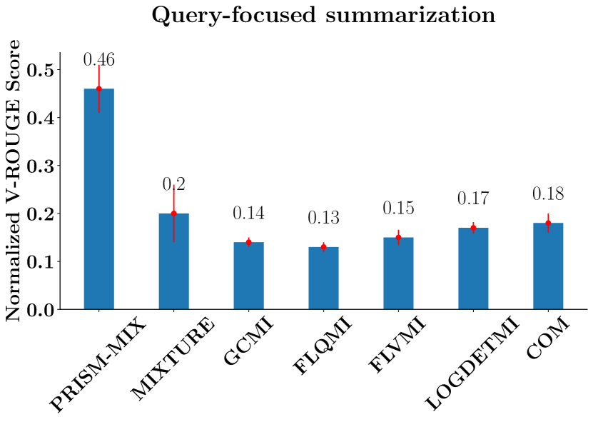
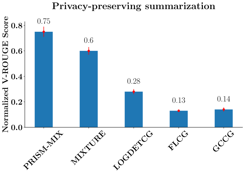
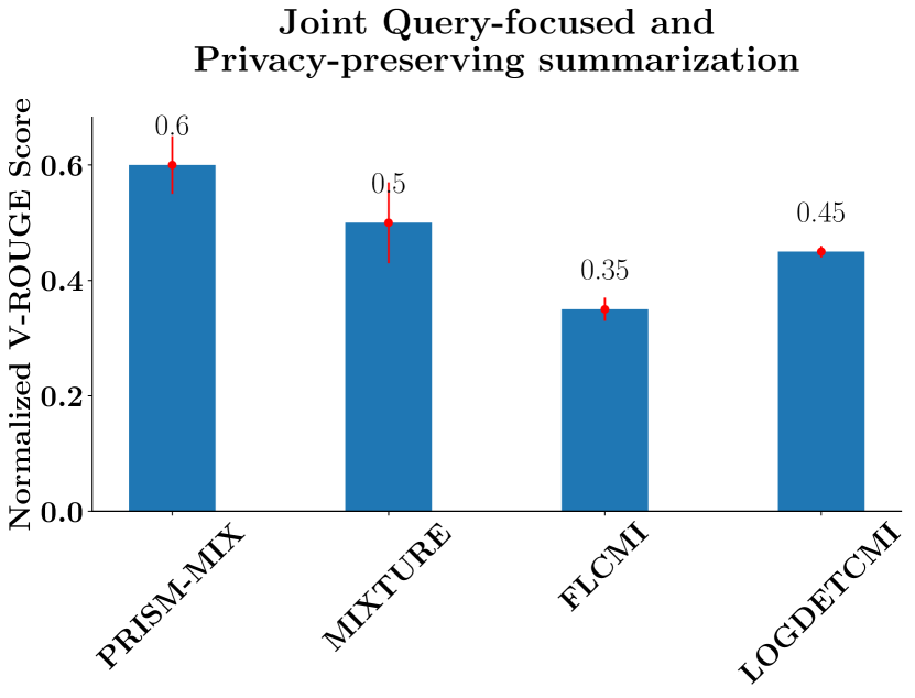
Figure 4: Guided summarization results on a real-world image collections dataset: because of the joint learning of the parameters, the proposed model (Prism-Mix) outperforms others in all flavors of summarization.

Baselines and Implementation details: We compare use of MI and CMI functions in Algo. 1 with other existing approaches. Specifically, for MI functions we use Logdetmi, Gcmi, Flvmi and, Flqmi. As baselines, we consider acquisition functions from the active learning literature; viz., entropy sampling (Entropy), Badge (Ash et al. 2020), and Glister-Active (Killamsetty et al. 2020). We run the active learning baselines only for one iteration to be consistent with our targeted learning setting (i.e., we select from the unlabeled set only once). Since these active learning baselines do not explicitly have information of the target set, to further strengthen the comparison, we also compare against two variants that are target-aware. The first is ‘targeted entropy sampling’ (Entropy-Tss), where a product of the uncertainty and the similarity with the target is used to identify the subset, and the second is Glister for targeted subset selection (Glister-Tss), where the target set is used in the bi-level optimization. We also compare against Grad-Match (Killamsetty et al. 2021), which mines for a subset such that the weighted difference in the gradients with the target set is minimized. Lastly, we also include vanilla FL and random sampling as baselines. For all datasets except MNIST, we train a ResNet-18 model (He et al. 2016). For MNIST, we train a LeNet model (LeCun et al. 1989). We use the cross-entropy loss and the SGD optimizer until training accuracy exceeds 99%. After augmenting the train set with the labeled version of the selected subset and re-training the model, we report the average gain in accuracy for the target classes and the overall gain in accuracy across all classes. The numbers reported are averaged over 10 runs of randomly picking any two classes for the target. We run Algo. 1 for different budgets and also study the effect of budget on the performance. We set the internal parameters to default values of 1. All experiments were run on an NVIDIA RTX 2080Ti GPU.

Results: We report the effect of budget on the average gain in accuracy of the target classes in Fig. 3(a-d). On all datasets, MI functions yield the best improvement in terms of accuracy on the target classes, viz., $\approx$ 20-30% gain over the model’s performance before re-training with the added targeted subset. While this gain is $\approx$ 12% higher than that of other methods, this also simultaneously improves the overall accuracy by $\approx$ 2-10% over other methods. Owing to their richer modeling, the MI functions consistently outperform all baselines across all budgets. This is also evident by the fact that MI functions select the most number of data points from the targeted classes (see Fig. 3(e-f)). Further, recall the discussion on the behavior of different MI functions in Section 2. As expected, Flvmi, Flqmi and Logdetmi functions that model both query-relevance and diversity, perform better than a) functions which tend to prefer relevance (viz., Gcmi, Entropy-Tss) and b) functions which tend to prefer diversity/representation (viz., Badge and FL). Also, we observe that as the budget is increased, the MI functions outperform other methods by greater margins on the target class accuracy (Fig. 3). We run targeted learning for higher budgets on all datasets, and we observe that the MI functions achieve $20\times$ to $50\times$ labeling efficiency in obtaining the same accuracy on rare classes when compared to random and $2\times$ to $4\times$ compared to the best performing baseline (see Appendix H for more details). Additionally, we perform an ablation study to compare the performance of MI functions with the CMI functions and observe that they are at par with each other (see Fig. 3(g-i)). Finally, we do a pairwise t-test to compare the performance of all methods and observe that the MI functions (particularly Flvmi and Flqmi) statistically significantly outperform all baselines (see Appendix H). From a computational perspective, Flqmi and Gcmi are the fastest in terms of running time and scalability and hence Flqmi is the preferred MI function given its scalability and consistent performance.

4.2 Guided Summarization

Dataset and Implementation Details: We use the image-collections dataset of (Tschiatschek et al. 2014). The dataset has 14 image collections with 100 images each and provides  50-250 human summaries per collection. We extend it by acquiring dense noun concept annotations (objects and scenes) for every image by pseudo-labelling using pre-trained off-the-shelf networks (Yolov3 pre-trained on OpenImagesv6 and ResNet50 pre-trained on Place365) followed by human correction. We designed query and private sets in a spirit similar to (Sharghi, Laurel, and Gong 2017) and acquired query-focused, privacy-preserving, and joint query-focused and privacy-preserving human summaries for every image collection. To instantiate the mixture model components, we extract concepts from images using the aforementioned pre-trained off-the-shelf networks and represent them, as well as the concept queries, by a $|\mathcal{C}|$-dimensional vector, where $\mathcal{C}$ is the universe of concepts. Our mixture model (Prism-Mix) has four components which are the appropriate instantiations (MI/CG/CMI) of functions - GC, LogDet, FL and COM. The mixture weights as well as the internal parameters ($\lambda,\nu,\eta$) are learned using the train set. Following (Tschiatschek et al. 2014), we perform leave-one-out cross validation and report average V-ROUGE across 14 runs. We also normalize V-ROUGE s.t. the human average is 1 and the random average is 0. We provide further details of the dataset and implementation in Appendix I.

Results: We present the guided summarization results in Fig. 4. As discussed in Section 3.3, the individual components of our mixture model have been used as models in previous works on document and video summarization. Hence, we compare the performance of Prism-Mix against the performance of the individual components as our baselines. Also, to confirm the positive effect of jointly learning the parameters of Prism along with the mixture weights, we compare Prism-Mix against a mixture model (Mixture) of exactly the same components, but with only the model weights $w$ being learned. Other internal parameters ($\lambda,\eta,\nu$) are set to fixed values of 1. We observe that Prism-Mix outperforms other techniques, including Mixture on all flavors of summarization (see Fig. 4). This is expected, as the joint learning of parameters offered by Prism (Sec. 3.2) enables producing summaries that can better imitate the complexities of the ground-truth summaries.

5 Conclusion

We presented Prism, a rich class of functions for guided subset selection. Prism allows to model a broad spectrum of semantics across query-relevance, diversity, query-coverage and privacy-irrelevance. We demonstrated its effectiveness in targeted learning as well as in guided summarization. We showed that Prism has interesting connections to several past work, further reinforcing its utility. Through several experiments on targeted learning and guided summarization for diverse datasets, we empirically verified the superiority of Prism over existing methods.

Appendix

Appendix A Summary of Notations

We present a summary of notations used throughout this paper in Table 2

Topic	Notation	Explanation
	$\mathcal{V}$	Ground set of $n$ instances
Prism	$\mathcal{V}^{\prime}$	Auxiliary set containing private set or query set
	$\Omega$	$\mathcal{V}\cup\mathcal{V}^{\prime}$
	$\mathcal{A}$	A subset of $\mathcal{V}$
	$S_{\mathcal{A},\mathcal{B}}$	Cross-similarity matrix between the items in sets $\mathcal{A}$ and $\mathcal{B}$
	$S_{\mathcal{A}\mathcal{B}}$	Similarity matrix for items in $\mathcal{A}\cup\mathcal{B}$
	$\lambda$	Parameter governing trade-off between representation and diversity in GC
	$\eta$	Parameter governing trade-off between query-relevance and diversity in MI and CMI functions
	$\nu$	Parameter governing hardness of privacy constraints in CG and CMI functions
	$\mathcal{E}$	Initial set of $|\mathcal{E}|$ labeled instances
Prism for Task 1: Improving a model’s accuracy (Algo. 1)	$\mathcal{U}$	Set of $|\mathcal{U}|$ instances in unlabeled data set
	${\mathcal{T}}$	Set of $|{\mathcal{T}}|$ instances in the target/query set
	$\gamma g(\mathcal{A})$	Diversity function that can be added to MI function in Algorithm 1 with weight $\gamma$
	$\mathcal{P}$ (as ${\mathcal{T}}$)	Private set or conditioning set for targeted summarization
Prism for Task 2: Targeted summarization	$\mathcal{Q}$ (as ${\mathcal{T}}$)	Query set for targeted summarization
	$\mathcal{F}(\Theta)$	Mixture model using Prism with parameters $\Theta$
	$\mathcal{L}_{n}(\Theta)$	Generalized hinge loss of training example $n$, with parameter $\Theta=({\bm{w}},\eta,\lambda,\nu)$

Table 2: Summary of notations used throughout this paper

Appendix B Proofs for Generalized Submodular Mutual Information (GMI) Functions - Restricted Submodularity

B.1 Properties of Generalized Submodular Mutual Information Functions

Lemma 1

Given a restricted submodular function $f$ on $\mathcal{C}(\mathcal{V},\mathcal{V}^{\prime})$, $I_{f}(\mathcal{A};\mathcal{B})\geq 0$ for $\mathcal{A}\subseteq\mathcal{V},\mathcal{B}\subseteq\mathcal{V}^{\prime}$. Also, $I_{f}(\mathcal{A};\mathcal{B})$ is monotone in $\mathcal{A}\subseteq\mathcal{V}$ for fixed $\mathcal{B}\subseteq\mathcal{V}^{\prime}$ (equivalently, $I_{f}(\mathcal{A};\mathcal{B})$ is monotone in $\mathcal{B}\subseteq\mathcal{V}^{\prime}$ for fixed $\mathcal{A}\subseteq\mathcal{V}$).

Proof  The non-negativity of the generalized submodular mutual information follows from the definition. In particular, since $\mathcal{A}\subseteq\mathcal{V}$ and $\mathcal{B}\subseteq\mathcal{V}^{\prime}$, it holds that

$$I_{f}(\mathcal{A};\mathcal{B})=f(\mathcal{A})+f(\mathcal{B})-f(\mathcal{A}\cup\mathcal{B})\geq 0$$

because $f$ is restricted submodular on $C(\mathcal{V},\mathcal{V}^{\prime})$. Next, we prove the monotonicity. We have,

$$I_{f}(\mathcal{A}\cup j;\mathcal{B})-I_{f}(\mathcal{A};\mathcal{B})=[f(j|\mathcal{A})-f(j|\mathcal{A}\cup\mathcal{B})],\forall j\in\mathcal{V}\backslash A$$

Given that $f$ is restricted submodular on $\mathcal{C}(\mathcal{V},\mathcal{V}^{\prime})$, it holds that

$$[f(j|\mathcal{A})-f(j|\mathcal{A}\cup\mathcal{B})]\geq 0$$

since

$$f(\mathcal{A}\cup\{j\})+f(\mathcal{A}\cup\mathcal{B})\geq f(\mathcal{A})+f(\mathcal{A}\cup\mathcal{B}\cup j)$$

which follows since the submodularity inequality holds as long as one of the sets is a subset of either $\mathcal{V}$ or $\mathcal{V}^{\prime}$ (i.e. both subsets do not non-empty intersection with $\mathcal{V}$ and $\mathcal{V}^{\prime}$. Thus

$$I_{f}(\mathcal{A}\cup\{j\};\mathcal{B})-I_{f}(\mathcal{A};\mathcal{B})\geq 0$$

and hence monotone.  

B.2 Concave Over Modular as GMI

Restating Lemma 1

The function $f_{\eta}(\mathcal{A})$ is a restricted submodular function on $\mathcal{C}(\mathcal{V},\mathcal{V}^{\prime})$. Furthermore, the GMI with $f_{\eta}$ is exactly $I_{f_{\eta}}(\mathcal{A};\mathcal{Q})=\eta\sum_{i\in\mathcal{A}}\psi(\sum_{j\in\mathcal{Q}}S_{ij})+\sum_{j\in\mathcal{Q}}\psi(\sum_{i\in\mathcal{A}}S_{ij})$, given a kernel matrix which satisfies $S_{ij}=1(i==j)$ for $i,j\in\mathcal{V}$ or $i,j\in\mathcal{V}^{\prime}$. The CG and CMI expressions are not particularly useful in this case.

Proof  Assume that the kernel matrix $S_{ij}\leq 1,\forall i,j\in\Omega$. Also, we are given that $S_{ij}=1(i==j)$ for $i,j\in\mathcal{V}$ or $i,j\in\mathcal{V}^{\prime}$. Next, notice that:

$$f(\mathcal{A})=\eta\sum_{i\in\mathcal{V}^{\prime}}\psi(\sum_{j\in\mathcal{A}}S_{ij})+\sum_{i\in\mathcal{A}}\psi(\sqrt{n})$$ (1)

This holds because the $S$ kernel is an identity kernel within $\mathcal{V}$ and $\mathcal{V}^{\prime}$ and only has terms in the cross between the two sets. Similarly,

$$f(\mathcal{Q})=\sum_{i\in\mathcal{V}}\psi(\sum_{j\in\mathcal{Q}}S_{ij})+\eta\sum_{i\in\mathcal{Q}}\psi(\sqrt{n})$$ (2)

Finally, we obtain $f(\mathcal{A}\cup\mathcal{Q})$:

$$f(\mathcal{A}\cup\mathcal{Q})=\eta\sum_{i\in\mathcal{V}^{\prime}\setminus\mathcal{Q}}\psi(\sum_{j\in\mathcal{A}}S_{ij})+\eta\sum_{i\in\mathcal{Q}}\psi(\sqrt{n})+\sum_{i\in\mathcal{V}\setminus\mathcal{A}}\psi(\sum_{j\in\mathcal{Q}}S_{ij})+\sum_{i\in\mathcal{A}}\psi(\sqrt{n})$$ (3)

Combining all the three terms together, we obtain $f(\mathcal{A})+f(\mathcal{Q})-f(\mathcal{A}\cup\mathcal{Q})=\eta\sum_{i\in\mathcal{A}}\psi(\sum_{j\in\mathcal{Q}}S_{ij})+\sum_{j\in\mathcal{Q}}\psi(\sum_{i\in\mathcal{A}}S_{ij})=F_{\eta}(\mathcal{A};\mathcal{Q})$.

Finally, to show that $f_{\eta}(S)$ is restricted submodular, notice that $f(\mathcal{A})$ is submodular if $\mathcal{A}$ is restricted to either $\mathcal{V}$ or $\mathcal{V}^{\prime}$. Similarly, given sets $\mathcal{A}\subseteq\mathcal{V},\mathcal{B}\subseteq\mathcal{V}^{\prime}$, it holds that $f(\mathcal{A})+f(\mathcal{B})-f(\mathcal{A}\cup\mathcal{B})=I_{f}(\mathcal{A};\mathcal{B})\geq 0$ which implies the restricted submodularity of $f_{\eta}(S)$.

Like FL (v2), the expressions for CG and CMI don’t make sense in COM since they require computing terms over $\mathcal{V}^{\prime}$, which we do not have access to.  

Appendix C Proofs for instantiations used in Prism

C.1 Log-Determinant Based Information Measures: Logdetmi, Logdetcg and Logdetcmi

Lemma 2

Setting $f(\mathcal{A})=\log\det(S_{\mathcal{A}})$, we have: $I_{f}(\mathcal{A};\mathcal{Q})=\log\det(S_{\mathcal{A}})-\log\det(S_{\mathcal{A}}-\eta^{2}S_{\mathcal{A},\mathcal{Q}}S_{\mathcal{Q}}^{-1}S_{\mathcal{A},\mathcal{Q}}^{T})$, and $f(\mathcal{A}|\mathcal{P})=\log\det(S_{\mathcal{A}}-\nu^{2}S_{\mathcal{A},\mathcal{P}}S_{\mathcal{P}}^{-1}S_{\mathcal{A},\mathcal{P}}^{T})$. Similarly, $I_{f}(\mathcal{A};\mathcal{Q}|\mathcal{P})=\log\frac{\det(I-S_{\mathcal{P}}^{-1}S_{\mathcal{P},\mathcal{Q}}S_{\mathcal{Q}}^{-1}S_{\mathcal{P},\mathcal{Q}}^{T})}{\det(I-S_{\mathcal{A}\mathcal{P}}^{-1}S_{\mathcal{A}\mathcal{P},\mathcal{Q}}S_{\mathcal{Q}}^{-1}S_{\mathcal{A}\mathcal{P},\mathcal{Q}}^{T})}$

Proof  Given a positive semi-definite matrix $S$, the Log-Determinant Function is $f(\mathcal{A})=\log\det(S_{\mathcal{A}})$ where $S_{\mathcal{A}}$ is a sub-matrix comprising of the rows and columns indexed by $\mathcal{A}$. The following expressions follow directly from the definitions. The MI is: $I_{f}(\mathcal{A};\mathcal{Q})=\log\frac{\det(S_{\mathcal{A}})\det(S_{\mathcal{Q}})}{\det(S_{\mathcal{A}\cup\mathcal{Q}})}$, CG is: $f(\mathcal{A}|\mathcal{P})=\log\frac{\det(S_{\mathcal{A}\cup\mathcal{P}})}{\det(S_{\mathcal{P}})}$ and CMI is $I_{f}(\mathcal{A};\mathcal{Q}|\mathcal{P})=\log\frac{\det(S_{\mathcal{A}\cup\mathcal{P}})\det(S_{Q\cup\mathcal{P}})}{\det(S_{\mathcal{A}\cup\mathcal{Q}\cup\mathcal{P}})\det(S_{\mathcal{P}})}$.

Next, note that using the Schur’s complement, $\det(S_{\mathcal{A}\cup\mathcal{B}})=\det(S_{\mathcal{A}})\det(S_{\mathcal{A}\cup\mathcal{B}}\backslash S_{\mathcal{A}})$ where,

$$S_{\mathcal{A}\cup\mathcal{B}}\backslash S_{\mathcal{A}}=S_{\mathcal{B}}-S_{\mathcal{A}\mathcal{B}}^{T}S_{\mathcal{A}}^{-1}S_{\mathcal{A}\mathcal{B}}$$

where $S_{\mathcal{A}\mathcal{B}}$ is a $|\mathcal{A}|\times|\mathcal{B}|$ matrix and includes the cross similarities between the items in sets $\mathcal{A}$ and $\mathcal{B}$. Similarly,

$$S_{\mathcal{A}\cup\mathcal{B}}\backslash S_{\mathcal{B}}=S_{\mathcal{A}}-S_{\mathcal{A}\mathcal{B}}S_{\mathcal{B}}^{-1}S_{\mathcal{A}\mathcal{B}}^{T}$$

As a result, the Mutual Information becomes:

$$I_{f}(\mathcal{A};\mathcal{Q}) =-\log[\det(S_{\mathcal{A}}-S_{\mathcal{A}\mathcal{Q}}S_{\mathcal{Q}}^{-1}S_{\mathcal{A}\mathcal{Q}}^{T})\det(S_{\mathcal{A}}^{-1})]$$

$$=-\log\det(I-S_{\mathcal{A}\mathcal{Q}}S_{\mathcal{Q}}^{-1}S_{\mathcal{A}\mathcal{Q}}^{T}S_{\mathcal{A}}^{-1})$$

$$=-\log\det(I-S_{\mathcal{A}}^{-1}S_{\mathcal{A}\mathcal{Q}}S_{\mathcal{Q}}^{-1}S_{\mathcal{A}\mathcal{Q}}^{T})$$

For the CG,

$$f(\mathcal{A}|\mathcal{P}) =f(\mathcal{A})-I_{f}(\mathcal{A};\mathcal{P})$$

$$=\log\det(S_{\mathcal{A}})-\log\det(S_{\mathcal{A}})+\log\det(S_{\mathcal{A}}-S_{\mathcal{A}\mathcal{Q}}S_{\mathcal{Q}}^{-1}S_{\mathcal{A}\mathcal{Q}}^{T})$$

$$=\log\det(S_{\mathcal{A}}-S_{\mathcal{A}\mathcal{Q}}S_{\mathcal{Q}}^{-1}S_{\mathcal{A}\mathcal{Q}}^{T})$$

Similarly, the proof of the conditional submodular mutual information follows from the simple observation that:

$$I_{f}(\mathcal{A};\mathcal{Q}|\mathcal{P})=I_{f}(\mathcal{A}\cup\mathcal{P};\mathcal{Q})-I_{f}(\mathcal{Q};\mathcal{P})$$

Plugging in the expressions of the mutual information of the log-determinant function, from above, we have,

$$I_{f}(\mathcal{A}\cup\mathcal{P};\mathcal{Q}) =-\log\det(I-S_{\mathcal{A}\cup\mathcal{P}}^{-1}S_{\mathcal{A}\cup\mathcal{P}Q}S_{\mathcal{Q}}^{-1}S_{\mathcal{A}\cup\mathcal{P}Q}^{T})$$

$$I_{f}(\mathcal{Q};\mathcal{P}) =-\log\det(I-S_{\mathcal{Q}}^{-1}S_{\mathcal{Q}\mathcal{P}}S_{\mathcal{P}}^{-1}S_{\mathcal{Q}\mathcal{P}}^{T})$$

$$\therefore I_{f}(\mathcal{A};\mathcal{Q}|\mathcal{P}) =\log\det(I-S_{\mathcal{P}}^{-1}S_{\mathcal{P},\mathcal{Q}}S_{\mathcal{Q}}^{-1}S_{\mathcal{P},\mathcal{Q}}^{T})-\log\det(I-S_{\mathcal{A}\cup\mathcal{P}}^{-1}S_{\mathcal{A}\cup\mathcal{P},Q}S_{\mathcal{Q}}^{-1}S_{\mathcal{A}\cup\mathcal{P},Q}^{T})$$

$$=\log\frac{\det(I-S_{\mathcal{P}}^{-1}S_{\mathcal{P},\mathcal{Q}}S_{\mathcal{Q}}^{-1}S_{\mathcal{P},\mathcal{Q}}^{T})}{\det(I-S_{\mathcal{A}\cup\mathcal{P}}^{-1}S_{\mathcal{A}\cup\mathcal{P},\mathcal{Q}}S_{\mathcal{Q}}^{-1}S_{\mathcal{A}\cup\mathcal{P},\mathcal{Q}}^{T})}$$

 

The proof for CMI implicitly assumes $\eta=\nu=1$. A simple way to solve this, is as follows. Denote $S_{\mathcal{A}\mathcal{P}\nu}$ as the similarity matrix obtained by multiplying $\nu$ to the cross similarity entries. Similarly, denote $S_{\mathcal{A}\mathcal{P}\nu,\mathcal{Q}\eta}$ as the cross similarity obtained by multiplying $\nu$ to the cross similarity between $\mathcal{A}$ and $\mathcal{P}$ and $\eta$ to the cross similarity between $\mathcal{A}$ and $\mathcal{Q}$. The CMI function with this choice of a similarity matrix is:

$$I_{f}(\mathcal{A};\mathcal{Q}|\mathcal{P})=\log\frac{\det(I-S_{\mathcal{P}}^{-1}S_{\mathcal{P},\mathcal{Q}}S_{\mathcal{Q}}^{-1}S_{\mathcal{P},\mathcal{Q}}^{T})}{\det(I-S_{\mathcal{A}\mathcal{P}\nu}^{-1}S_{\mathcal{A}\mathcal{P}\nu,\mathcal{Q}\eta}S_{\mathcal{Q}}^{-1}S_{\mathcal{A}\mathcal{P}\nu,\mathcal{Q}\eta}^{T})}$$ (4)

C.2 Facility Location based Information Measures: Flvmi, Flqmi, Flcg

Theorem 1

Given a similarity kernel $S$, a set $\mathcal{U}\subseteq\Omega$ and the facility location (FL) function $f(\mathcal{A})=\sum_{i\in\mathcal{U}}\max_{j\in\mathcal{A}}S_{ij},\mathcal{A}\subseteq\Omega$ the Mutual Information for FL can be written as $I_{f}(\mathcal{A};\mathcal{Q})=\sum_{i\in\mathcal{U}}\min(\max_{j\in\mathcal{A}}S_{ij},\max_{j\in\mathcal{Q}}S_{ij})$. Similarly, the CG for facility location can be written as $f(\mathcal{A}|P)=\sum_{i\in\mathcal{U}}\max(\max_{j\in\mathcal{A}}S_{ij}-\max_{j\in P}S_{ij},0)$ and the expression for Conditional Submodular Mutual Information can be written as: $I_{f}(\mathcal{A};\mathcal{Q}|\mathcal{P})=\sum_{i\in\mathcal{U}}\max(\min(\max_{j\in\mathcal{A}}S_{ij},\max_{j\in\mathcal{Q}}S_{ij})-\max_{j\in P}S_{ij},0)$.

Proof  Here we have the facility location set function, $f(\mathcal{A})=\sum_{i\in\mathcal{U}}\max_{j\in\mathcal{A}}S_{ij}$ where $s$ is similarity kernel and $U\subseteq\Omega$. Then,

$$I_{f}(\mathcal{A};\mathcal{Q}) =f(\mathcal{A})+f(\mathcal{Q})-f(\mathcal{A}\cup\mathcal{Q})$$

$$=\sum_{i\in\mathcal{U}}\max_{j\in\mathcal{A}}S_{ij}+\max_{j\in\mathcal{Q}}S_{ij}-\max_{j\in\mathcal{A}\cup\mathcal{Q}}S_{ij}$$

$$=\sum_{i\in\mathcal{U}}\max_{j\in\mathcal{A}}S_{ij}+\max_{j\in\mathcal{Q}}S_{ij}-\max(\max_{j\in\mathcal{A}}S_{ij},\max_{j\in\mathcal{Q}}S_{ij})$$

$$=\sum_{i\in\mathcal{U}}\min(\max_{j\in\mathcal{A}}S_{ij},\max_{j\in\mathcal{Q}}S_{ij})$$

For the Conditional Gain we have

$$f(\mathcal{A}|\mathcal{P}) =\sum_{i\in\mathcal{U}}\max(\max_{j\in\mathcal{A}}S_{ij},\max_{j\in\mathcal{P}}S_{ij})-\max_{j\in\mathcal{P}}S_{ij}$$

$$=\sum_{i\in\mathcal{U}}\max(0,\max_{j\in\mathcal{A}}S_{ij}-\max_{j\in\mathcal{P}}S_{ij})$$

Finally, we can get the expression for $I_{f}(\mathcal{A};\mathcal{Q}|\mathcal{P})$ as

$$I_{f}(\mathcal{A};\mathcal{Q}|\mathcal{P}) =f(\mathcal{A}|\mathcal{P})+f(\mathcal{Q}|\mathcal{P})-f(\mathcal{A}\cup\mathcal{Q}|\mathcal{P})$$

$$=\sum_{iinU}[\max(\max_{jin\mathcal{A}}S_{ij}-\max_{jin\mathcal{P}}S_{ij},0)+\max(\max_{j\in\mathcal{Q}}S_{ij}-\max_{j\in\mathcal{P}}S_{ij},0)-\max(\max_{j\in\mathcal{A}\cup\mathcal{Q}}S_{ij}-\max_{j\in P}S_{ij},0)]$$

$$=\sum_{i\in\mathcal{U}}\max(\min(\max_{j\in\mathcal{A}}S_{ij},\max_{j\in\mathcal{Q}}S_{ij})-\max_{j\in P}S_{ij},0)$$

The last step follows from the observation that in $\max(a-c,0)+\max(b-c,0)-\max(\max(a,b)-c,0)$ the last term is either the first term or the second term (hence cancelling that out) depending on whether $a>b$ or not.  
Now, we can obtain the expression of Flvmi, Flqmi, Flcg and Flcmi as special cases.

Corollary 1

Setting $U=V$ in the expression of MI, CG and CMI in Theorem 1, we obtain the expression for Flvmi as $I_{f}(\mathcal{A};\mathcal{Q})=\sum_{i\in\mathcal{V}}\min(\max_{j\in\mathcal{A}}S_{ij},\max_{j\in\mathcal{Q}}S_{ij})$, Flcg as $f(\mathcal{A}|\mathcal{P})=\sum_{i\in\mathcal{V}}\max(\max_{j\in\mathcal{A}}S_{ij}-\max_{j\in\mathcal{P}}S_{ij},0)$ and Flcmi as $I_{f}(\mathcal{A};\mathcal{Q}|\mathcal{P})=\sum_{i\in\mathcal{V}}\max(\min(\max_{j\in\mathcal{A}}S_{ij},\max_{j\in\mathcal{Q}}S_{ij})-\max_{j\in P}S_{ij},0)$

This corollary follows directly from Theorem 1. We can similarly, also obtain the expression for Flqmi.

Lemma 3

Given a similarity kernel $S$ such that $S_{ij}=I(i==j)$, if both $i,j\in\mathcal{V}$ or both $i,j\in\mathcal{V}^{\prime}$ and the facility location (FL) function $f(\mathcal{A})=\sum_{i\in\Omega}\max_{j\in\mathcal{A}}S_{ij},\mathcal{A}\subseteq\Omega$ we obtain the expression for MI (Flqmi) as $I_{f}(\mathcal{A};\mathcal{Q})=\sum_{i\in\mathcal{Q}}\max_{j\in\mathcal{A}}S_{ij}+\eta\sum_{i\in\mathcal{A}}\max_{j\in\mathcal{Q}}S_{ij}$. The CG and CMI expressions are not particularly useful in this case.

Proof  Assuming $s_{ii}=1$ is the maximum similarity score in the kernel, for the alternative formulation under the assumption that $U=\Omega$, we can break down the sum over elements in ground set $\Omega$ as follows. For any $i\in\mathcal{A},\max_{j\in\mathcal{A}}S_{ij}=1$ and hence the minimum (over sets $\mathcal{A}$ and $\mathcal{Q}$) will just be the term corresponding to Q (and a similar argument follows for terms in $\mathcal{Q}$). Then we have,

$$I_{f}(\mathcal{A};\mathcal{B}) =\sum_{i\in\Omega\setminus(\mathcal{A}\cup\mathcal{Q})}\min(\max_{j\in\mathcal{A}}S_{ij},\max_{j\in\mathcal{Q}}S_{ij})+\sum_{i\in\mathcal{A}\setminus\mathcal{Q}}\max_{j\in\mathcal{Q}}S_{ij}+\sum_{i\in\mathcal{Q}\setminus\mathcal{A}}\max_{j\in\mathcal{A}}S_{ij}+\sum_{i\in\mathcal{A}\cap\mathcal{Q}}1$$ (5)

$$=\sum_{i\in\mathcal{V}\setminus\mathcal{A}}\min(\max_{j\in\mathcal{A}}S_{ij},\max_{j\in\mathcal{Q}}S_{ij})+\sum_{i\in\mathcal{V}^{\prime}\setminus\mathcal{Q}}\min(\max_{j\in\mathcal{A}}S_{ij},\max_{j\in\mathcal{Q}}S_{ij})+\sum_{i\in\mathcal{A}}\max_{j\in\mathcal{Q}}S_{ij}+\sum_{i\in\mathcal{Q}}\max_{j\in\mathcal{A}}S_{ij}$$ (6)

This follows because $\mathcal{A}\cap\mathcal{Q}=\emptyset$. Finally, note that

$$\sum_{i\in\mathcal{V}\setminus\mathcal{A}}\min(\max_{j\in\mathcal{A}}S_{ij},\max_{j\in\mathcal{Q}}S_{ij})+\sum_{i\in\mathcal{V}^{\prime}\setminus\mathcal{Q}}\min(\max_{j\in\mathcal{A}}S_{ij},\max_{j\in\mathcal{Q}}S_{ij})=0$$

since $\forall i\in\mathcal{V}\setminus\mathcal{A},j\in\mathcal{A},S_{ij}=0$ and similarly $\forall i\in\mathcal{V}^{\prime}\setminus\mathcal{Q},j\in\mathcal{Q},S_{ij}=0$. This leaves us with $I_{f}(\mathcal{A};\mathcal{Q})=\sum_{i\in\mathcal{Q}}\max_{j\in\mathcal{A}}S_{ij}+\eta\sum_{i\in\mathcal{A}}\max_{j\in\mathcal{Q}}S_{ij}$

The expressions for CG and CMI don’t make sense in this version of FL since they require computing terms over $\mathcal{V}^{\prime}$, which we do not have access to.  

C.3 Expression for GCCMI is not useful

Lemma 4

When $f$ is the graph-cut function, $I_{f}(\mathcal{A};\mathcal{Q}|\mathcal{P})=I_{f}(\mathcal{A};\mathcal{Q})$. In other words, the CMI function does not depend on the private set $\mathcal{P}$.

Proof  For deriving the expression for Conditional Submodular Mutual Information we proceed as follows,

Let

$$g(\mathcal{A})=f(\mathcal{A}|P)=f(\mathcal{A})-2\lambda\sum_{i\in\mathcal{A}}\sum_{j\in P}S_{ij}$$

Then,

$$I_{f}(\mathcal{A};\mathcal{Q}|P) =I_{g}(\mathcal{A};\mathcal{Q})$$

$$=I_{f}(\mathcal{A};\mathcal{Q})-2\lambda\sum_{i\in\mathcal{A}\cap\mathcal{Q},j\in\mathcal{P}}S_{ij}$$

Since $\mathcal{A},\mathcal{Q}$ are disjoint, the second term is 0 and the first term doesn’t have any effect of $\mathcal{P}$. Thus, the Conditional Submodular Mutual Information for Graph Cut (GCCMI) isn’t useful.  

Appendix D Scalability of Prism

Below, we provide a detailed analysis of the complexity of creating and optimizing the different functions in Prism. Denote $|\mathcal{X}|$ as the size of set $\mathcal{X}$. Also, let $|\mathcal{U}|=n$ (the ground set size, which is the size of the unlabeled set in this case) and $B$ be the selection budget. In the main paper, we provided the high level intuition of the complexity, ignoring the terms of $|\mathcal{P}|$ and $|\mathcal{Q}|$ since they would be typically much smaller than the number of unlabeled points $n$. For completeness, we provide the detailed complexity below:

• Facility Location: We start with Flvmi. The complexity of creating the kernel matrix is $O(n^{2})$. The complexity of optimizing it is $\tilde{O}(n^{2})$ (using memoization (iyer2019memoization)) if we use the stochastic greedy algorithm (Mirzasoleiman et al. 2015) and $O(n^{2}k)$ with the naive greedy algorithm. The overall complexity is $\tilde{O}(n^{2})$. For Flqmi, the cost of creating the kernel matrix is $O(n|\mathcal{Q}|)$, and the cost of optimization is also $\tilde{O}(n|\mathcal{Q}|)$ (with naive greedy, it is $O(nB|\mathcal{Q}|)$). The complexity of Flcg is $O([n+|\mathcal{P}|]^{2})$ to compute the kernel matrix and $\tilde{O}(n^{2})$ for optimizing (using the stochastic greedy algorithm). Finally, for Flcmi, the complexity of computing the kernel matrix is $O([n+|\mathcal{Q}|+|\mathcal{P}|]^{2})$, and the complexity of optimization is $\tilde{O}(n^{2})$.

• Log-Determinant: We start with Logdetmi. The complexity of the kernel matrix computation (and storage) is $O(n^{2})$. The complexity of optimizing the LogDet function using the stochastic greedy algorithm is $\tilde{O}(B^{2}n)$, so the overall complexity is $\tilde{O}(n^{2}+B^{2}n)$. For Logdetcg, the complexity of computing the matrix is $O([n+|\mathcal{P}|]^{2}$, and the complexity of optimization is $\tilde{O}([B+|\mathcal{P}|]^{2}n)$. For the Logdetcmi function, the complexity of computing the matrix is $O([n+|\mathcal{P}|+|\mathcal{Q}|]^{2}$, and the complexity of optimization is $\tilde{O}([B+|\mathcal{P}|+|\mathcal{Q}|]^{2}n)$.

• Graph-Cut: Finally, we study GC functions. For Gcmi, we require an $O(n|\mathcal{Q}|)$ kernel matrix, and the complexity of the stochastic greedy algorithm is also $\tilde{O}(n|\mathcal{Q}|)$. Finally, for Gccg, the complexity of creating the kernel matrix is $O(n|^{2}+n|\mathcal{P}|)$, and the complexity of the stochastic greedy algorithm is $\tilde{O}(n^{2}+n|\mathcal{P}|)$.

We end with a few comments. First, most of the complexity analysis above is with the stochastic greedy algorithm (Mirzasoleiman et al. 2015). If we use the naive or lazy greedy algorithm, the worst-case complexity is a factor $B$ larger. Secondly, we ignore log-factors in the complexity of stochastic greedy since the complexity is actually $O(n\log 1/\epsilon)$, which achieves a $1-1/e-\epsilon$ approximation. Finally, the complexity of optimizing and constructing the FL, LogDet, and GC functions can be obtained from the CG versions by setting $\mathcal{P}=\emptyset$.

D.1 Details on Partitioning Approach

For larger datasets, we can choose to partition the unlabeled set into chunks in order to meet the scale of the dataset. This is because many of the techniques (specifically LogDet functions, Flvmi, Flcg, Flcmi, Gccg) all have $O(n^{2})$ space complexity. For $n$ in the range of a few million to a few billion data points (which is not uncommon in big-data applications today), we need to scale our algorithms to be linear in $n$ and not quadratic. For this, we propose a simple partitioning approach where the unlabeled data is chunked into $p$ partitions. In this strategy, we perform unlabeled instance acquisition on each chunk using a proportional fraction of the full budget. By performing acquisition on the full unlabeled set, almost all strategies will exhaust the available compute resources. Hence, to execute most selection strategies, we can partition the unlabeled set into equally sized chunks, such that each partition has around 10k to 20k instances. As $n$ grows, the number of partitions would also grow, so that $n/p$ is roughly constant. The complexity of most approaches discussed above would then be $O(n^{2}/p)$ ($O(n^{2}/p^{2})$ for each chunk, repeated $p$ times), and if $n/p=r$ is a constant, then the complexity $O(nr)$ would be linear in $n$. We then acquire a number of unlabeled instances from each chunk whose ratio with the full selection budget is equal to the ratio between the chunk size and the full unlabeled set. The acquired instances from each chunk are then combined to form the full acquired set of unlabeled instances.

Appendix E Prism Modeling a Broad Spectrum of Semantics

Here we provide additional details on our experiments for empirically studying the modeling capabilities of different functions in Prism and the role of different parameters.

E.1 Experimental Setup

We create a synthetic dataset to understand the behaviour of the different functions in Prism, and the corresponding control parameters. We generate 10 different collections of points in a 2D space that emulates the space of images and queries/private instances. In each collection, there are 100 points representing images, 8 points representing queries and 2 points representing the private instances. These 110 points in each set are distributed in 18 clusters with different number of points in each cluster. The standard deviation is varied from one set to another and the 8 query points and 2 private instances for each set are randomly sampled without replacement, one each from 10 randomly selected clusters.

For different functions in Prism and for different settings of the internal parameters we maximize the function to produce a summary and compute the relevant measures averaged across different budgets (5-40 in intervals of 5) and different collections.

Scoring Functions. To characterize query-focused and privacy-preserving summaries we define the following. Query-saturation is a phenomenon where the function doesn’t see any gains in picking more query-relevant items after having picked a few. Query Coverage is calculated as the fraction of query points covered by the summary and measures if a summary doesn’t starve any query by always picking elements matching some other queries. A query point is said to be covered by a summary if there exists a selection in the summary which belongs to the same cluster as the query point. We quantify the Diversity of a summary by calculating the fraction of unique clusters covered by the summary. Next, we define Query-Relevance to be the fraction of points selected which match some query point and we define Privacy-Irrelevance as the fraction of points selected which do not match any private instance.

Figure 5: Comparison of different functions in Prism and effect of parameters. All plots share the legend.

E.2 Additional Quantitative Results

In Fig. 5 (also in the main text) we presented the behavior of the first variant (v1) of FLMI, as we change the internal parameter $\eta$ (top-left). Here we present similar observations for other functions like Flqmi and Logdetmi (Fig. 6 a, b).

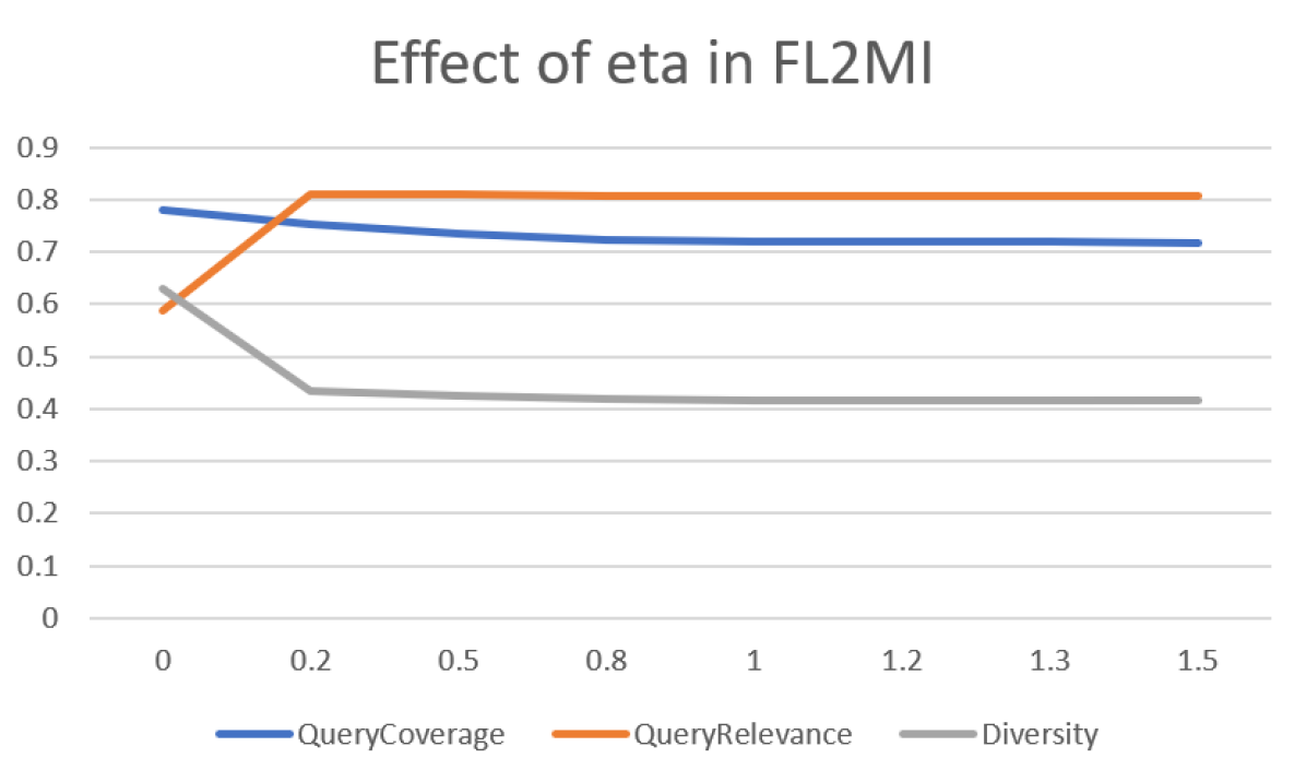
(a) Flqmi

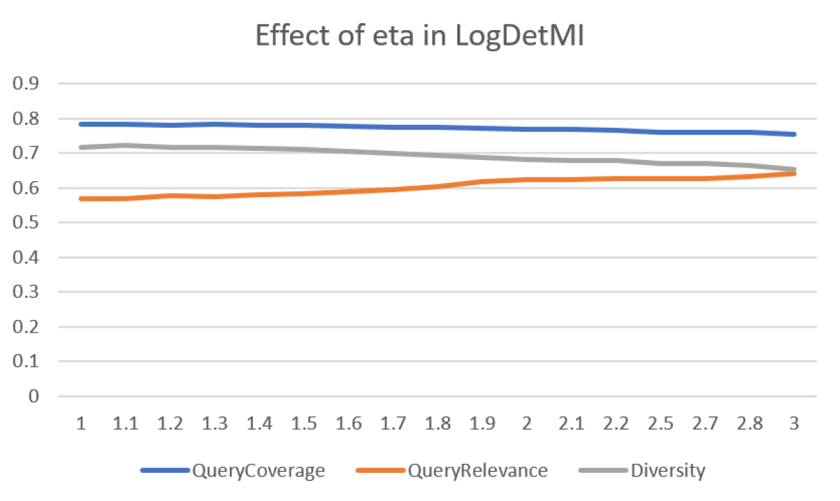
(b) Logdetmi

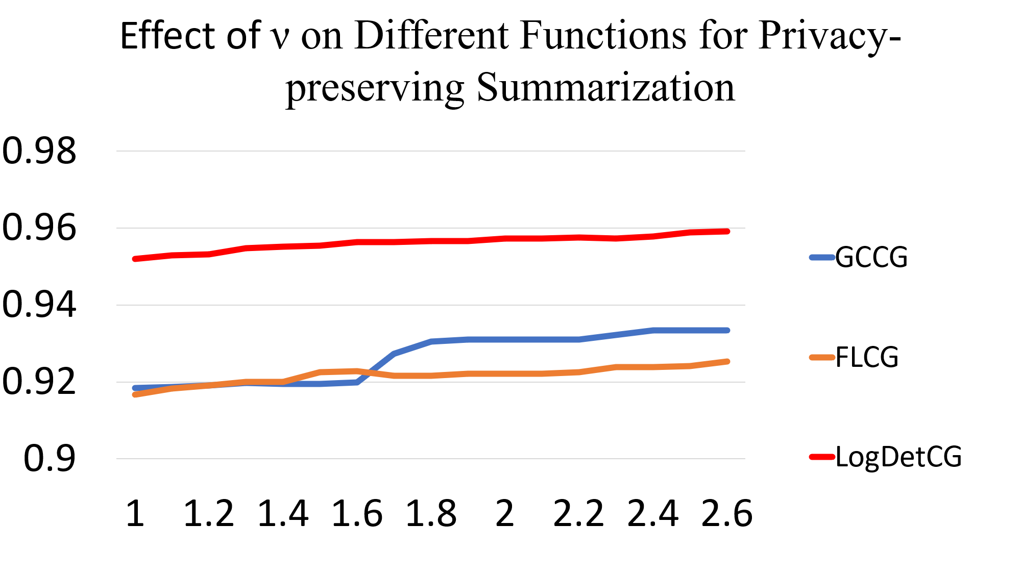
(c)

Figure 6: Effect of $\eta$ on (a)Flqmi and (b)Logdetmi and the effect of $\nu$ on different CG functions (c)

In Fig. 5 (top-right), we compare query-coverage, diversity and query-relevance for Gcmi, Flvmi and Flqmi, Logdetmi and COM, fixing the value of $\eta=1$ wherever applicable. In each case, we also compare a version which adds a very small diversity term to these functions (to measure the effect of saturation of the MI functions) (Fig. 7(a)). We make the following observations. Gcmi, Flqmi, Logdetmi and COM favor query-relevance over diversity and query-coverage, while Flvmi favors diversity and query-coverage over query-relevance. Furthermore, we also observe that COM does not change as much with the addition of diversity, which suggests that it is not saturated, while Logdetmi significantly changes its behaviour with the addition of diversity. In almost all cases, we see that adding a small diversity term reduces query-relevance in favor of query-coverage and diversity, which is also something we expect.

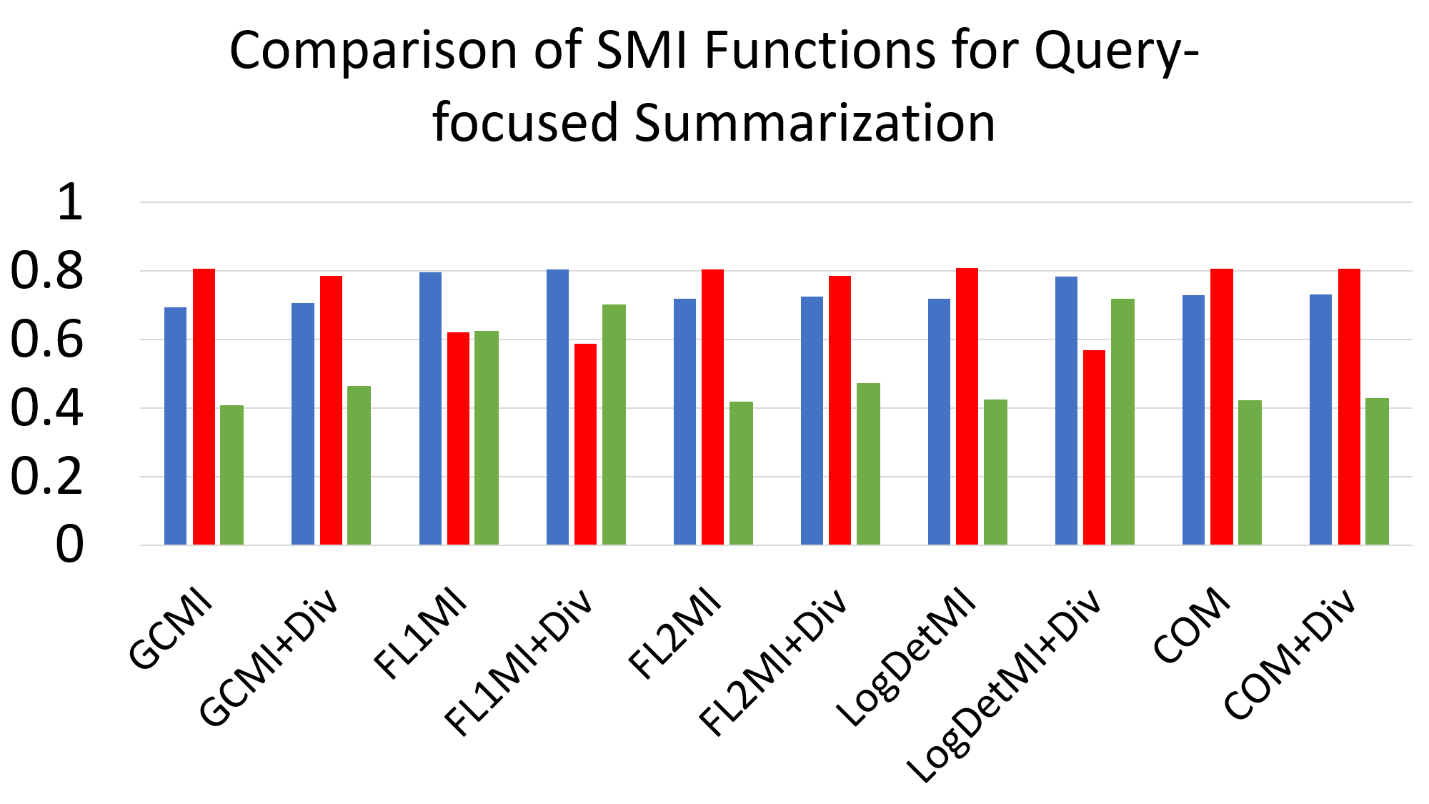
(a)

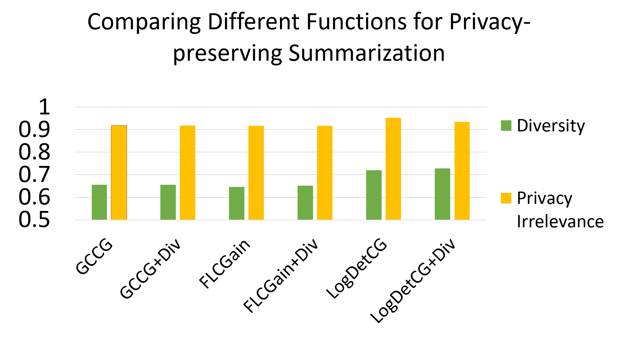
(b)

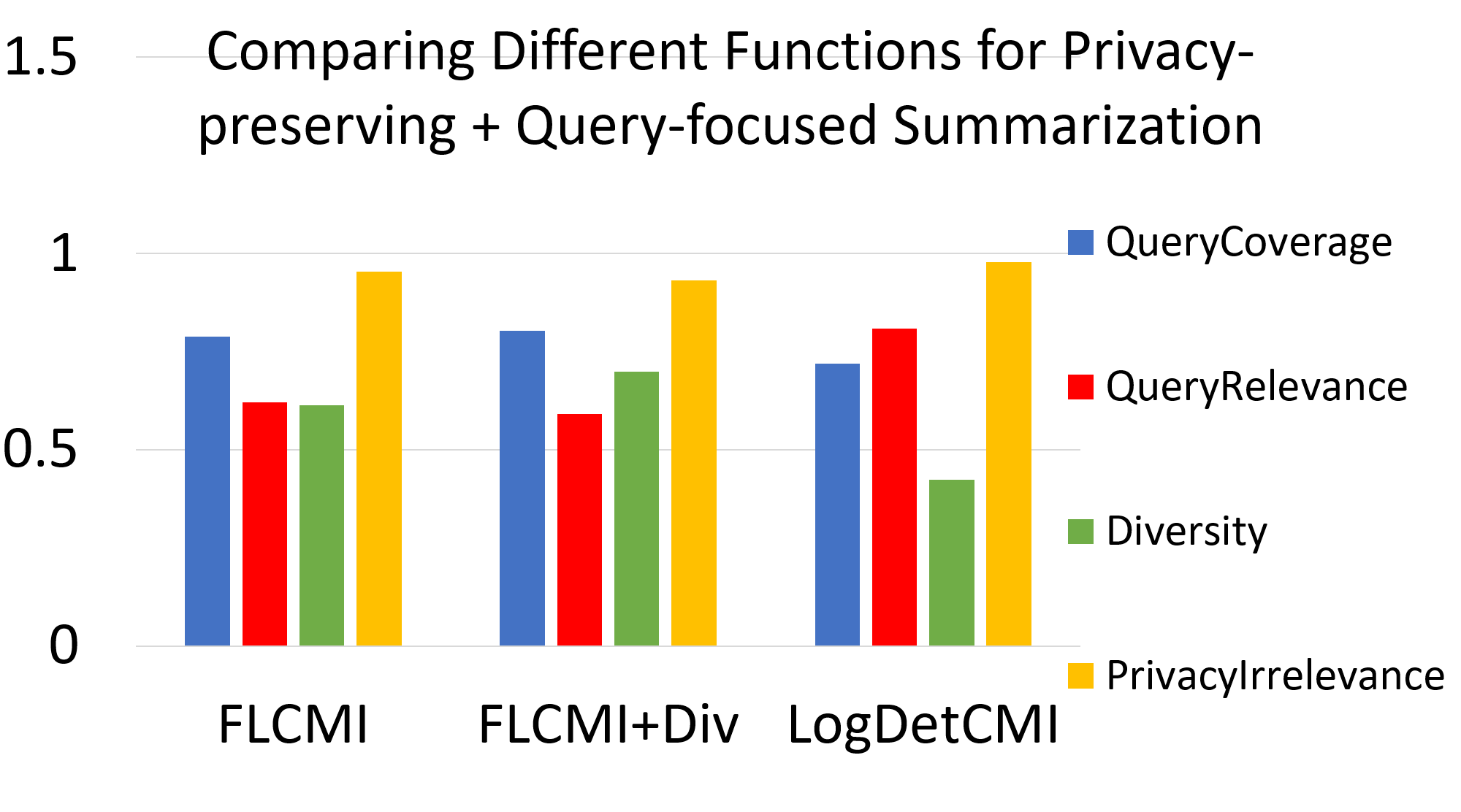
(c)

Figure 7: Behavior of different functions in Prism and effect of parameters. Different from Fig. 5, we also add a version which adds a very small diversity term to these functions (to measure the effect of saturation of the MI functions). See text for details.

Next, we report the results for privacy-preserving summarization. Fig. 6(c) shows the effect of $\nu$ on the privacy-irrelevance term in Gccg, Flcg and Logdetcg. As we expect, increasing $\nu$ increases the privacy-irrelevance score, thereby ensuring a stricter privacy-irrelevance constraint. Fig. 7(b) compares the Diversity and Privacy-Irrelevance score with different choices of functions (GC, FL and LogDet) for a fixed value $\nu=1$. Again, we also compare these to their variants where we add a small amount of diversity, and unlike the MI case, we see that the CG functions do not saturate and adding a small diversity does not change the selection. Finally, we see the trend here that Log-Det outperforms FL and GC both in terms of diversity and privacy irrelevance. In Fig. 7(c) we report the results for joint-summarization. We show the comparison for different functions (Flcmi, Flcmi + Div and Logdetcmi). Similar to the private and query versions, we observe that Flcmi tends to favor query-coverage and diversity in contrast to query-relevance and privacy-irrelevance, while Logdetcmi favors query-relevance and privacy-irrelevance over query-coverage and diversity.

E.3 Qualitative Analysis

In Fig. 8 we show the visualization of the 100 image points (black) and 8 query points (green) of collection number 3 in our synthetic dataset along with the 10 selected summary points (blue) selected by Flqmi at $\eta=0.0$ and $\eta=0.2$, labeled as per the order of their selection. F, R, D, I stand for Query-coverage, Query-relevance, Diversity and Privacy-irrelevance respectively. As discussed above, we can see that as soon as $\eta$ is increased, the summary produced by Flqmi becomes more query-relevant and less diverse.

(a) $\eta=0.0$

(b) $\eta=0.2$

Figure 8: Visualization of Flqmi behavior with varying $\eta$ on collection number 3 of the synthetic dataset

Appendix F Unified Learning Framework for Guided Summarization using Prism

Below we present the specific forms of the mixture model and the objective function and computation of gradients in the different cases of Generic, Query-Focused, Privacy-Preserving and Joint Summarization

Generic Summarization

We denote our dataset of $N$ training examples as $(\mathcal{Y}^{(n)},\mathcal{V}^{(n)},x^{(n)})$ where $n=1\dots N$, $\mathcal{Y}^{(n)}$ is a human summary for the $n^{th}$ ground set (image collection) $\mathcal{V}^{(n)}$ with features $x^{(n)}$.

We denote our mixture model in case of generic summarization as

$$F(Y,x^{(n)},w,\lambda)=\sum_{i=1}^{M}w_{i}f_{i}(Y,x^{(n)},\lambda_{i})$$

where $f_{1}\dots f_{M}$ are the instantiations of different submodular functions, $w_{i}$ their weights and $\lambda_{1}\dots\lambda_{M}$ are their internal parameters respectively, for example the $\lambda$ in case of Graph Cut function defined above.

So the parameters vector in case of generic summarization becomes $\Theta=(w_{1}\dots w_{m},\lambda_{1}\dots\lambda_{M})$

Then, $\mathcal{L}_{n}(\Theta)=\max_{Y\subset\mathcal{V}^{(n)},|\mathcal{Y}|\leq k}[\sum_{i=1}^{M}w_{i}f_{i}(Y,x^{(n)},\lambda_{i})+l_{n}(\mathcal{Y})]-\sum_{i=1}^{M}w_{i}f_{i}(\mathcal{Y}^{(n)},x^{(n)},\lambda_{i})$

For the purpose of learning the parameters $w_{i}$ and $\lambda_{i}$, we compute the gradients as,

$$\frac{\partial L_{n}}{\partial w_{i}}=f_{i}(\hat{Y_{n}},x^{(n)},\lambda_{i})-f_{i}(\mathcal{Y}^{(n)},x^{(n)},\lambda_{i})$$

and

$$\frac{\partial L_{n}}{\partial\lambda_{i}}=w_{i}\frac{\partial f_{i}(\hat{Y_{n}},x^{(n)},\lambda_{i})}{\partial\lambda_{i}}-w_{i}\frac{\partial f_{i}(\mathcal{Y}^{(n)},x^{(n)},\lambda_{i})}{\partial\lambda_{i}}$$

where

$$\hat{Y_{n}}=\mathop{\mathrm{argmax}}_{Y\subset\mathcal{V}^{(n)},|\mathcal{Y}|\leq k}F(Y,x^{(n)},w,\lambda)+l_{n}(\mathcal{Y})$$

For the gradients with respect to the respective internal parameters of individual function components $\frac{\partial f_{i}}{\partial\lambda_{i}}$, consider the generalized graphcut $f(Y,x^{(n)},\lambda)=\sum_{i\in\mathcal{V},j\in Y}S_{ij}^{(n)}-\lambda\sum_{i,j\in Y}S_{ij}^{(n)}$ as an example. We compute its gradient as,

$$\frac{\partial f(Y,x^{(n)},\lambda)}{\partial\lambda}=-\sum_{i,j\in Y}S_{ij}^{(n)}$$

Query-Focused Summarization

We denote our dataset of $N$ training examples as $(\mathcal{Y}^{(n)},\mathcal{V}^{(n)},x^{(n)},\mathcal{Q}^{(n)})$ where $n=1\dots N$, $\mathcal{Y}^{(n)}$ is a human query-summary for the query $\mathcal{Q}^{(n)}$ on the $n^{th}$ ground set (image collection) $\mathcal{V}^{(n)}$ with features $x^{(n)}$.

We denote our mixture model in case of query summarization as

$$F(Y,\mathcal{Q}^{(n)},x^{(n)},w,\lambda,\eta)=\sum_{i=1}^{M}w_{i}I_{f_{i}}(Y,\mathcal{Q}^{(n)},x^{(n)},\lambda_{i},\eta_{i})$$

where $f_{1}\dots f_{M}$ are the instantiations of different submodular mutual information functions, $w_{i}$ their weights, $\lambda_{1}\dots\lambda_{M}$ are their internal parameters respectively and $\eta_{1}\dots\eta_{M}$ are their query-relevance-diversity tradeoff parameters.

So the parameters vector in case of query-focused summarization becomes $\Theta=(w_{1}\dots w_{m},\lambda_{1}\dots\lambda_{M},\eta_{1}\dots\eta_{M})$

Then,

$$\mathcal{L}_{n}(\Theta)=\max_{Y\subset\mathcal{V}^{(n)},|\mathcal{Y}|\leq k}[\sum_{i=1}^{M}w_{i}I_{f_{i}}(Y,\mathcal{Q}^{(n)},x^{(n)},\lambda_{i},\eta_{i})+l_{n}(\mathcal{Y})]-\sum_{i=1}^{M}w_{i}I_{f_{i}}(\mathcal{Y}^{(n)},\mathcal{Q}^{(n)},x^{(n)},\lambda_{i},\eta_{i})$$

For the purpose of learning the parameters $w_{i}$, $\lambda_{i}$ and $\eta_{i}$ we compute the gradients as,

$$\frac{\partial L_{n}}{\partial w_{i}}=I_{f_{i}}(\hat{Y_{n}},\mathcal{Q}^{(n)},x^{(n)},\lambda_{i},\eta_{i})-I_{f_{i}}(\mathcal{Y}^{(n)},\mathcal{Q}^{(n)},x^{(n)},\lambda_{i},\eta_{i})$$

$$\frac{\partial L_{n}}{\partial\lambda_{i}}=w_{i}\frac{\partial I_{f_{i}}(\hat{Y_{n}},\mathcal{Q}^{(n)},x^{(n)},\lambda_{i},\eta_{i})}{\partial\lambda_{i}}-w_{i}\frac{\partial I_{f_{i}}(\mathcal{Y}^{(n)},\mathcal{Q}^{(n)},x^{(n)},\lambda_{i},\eta_{i})}{\partial\lambda_{i}}$$

and

$$\frac{\partial L_{n}}{\partial\eta_{i}}=w_{i}\frac{\partial I_{f_{i}}(\hat{Y_{n}},\mathcal{Q}^{(n)},x^{(n)},\lambda_{i},\eta_{i})}{\partial\eta_{i}}-w_{i}\frac{\partial I_{f_{i}}(\mathcal{Y}^{(n)},\mathcal{Q}^{(n)},x^{(n)},\lambda_{i},\eta_{i})}{\partial\eta_{i}}$$

where

$$\hat{Y_{n}}=\mathop{\mathrm{argmax}}_{Y\subset\mathcal{V}^{(n)},|\mathcal{Y}|\leq k}F(Y,\mathcal{Q}^{(n)},x^{(n)},w,\lambda,\eta)+l_{n}(\mathcal{Y})$$

For the gradients of individual function components $\frac{\partial I_{f_{i}}}{\partial\eta_{i}}$ with respect to the respective query-relevance-diversity trade-off parameters $\eta_{i}$, we show computation for some functions as follows:

Flvmi: $I_{f}(Y,\mathcal{Q}^{(n)},x^{(n)},\eta)=\sum_{i\in\mathcal{V}}\min(\max_{j\in Y}S_{ij}^{(n)},\eta\max_{j\in\mathcal{Q}^{(n)}}S_{ij}^{(n)})$

$$\frac{\partial I_{f}(Y,\mathcal{Q}^{(n)},x^{(n)},\eta)}{\partial\eta}=\sum_{i\in\mathcal{V}}(\max_{j\in\mathcal{Q}^{(n)}}S_{ij}^{(n)}*1_{\max_{j\in\mathcal{Q}^{(n)}}S_{ij}^{(n)}\leq\max_{j\in Y}S_{ij}^{(n)}})$$

Flqmi: $I_{f}(Y,\mathcal{Q}^{(n)},x^{(n)},\eta)=\sum_{i\in\mathcal{Q}^{(n)}}\max_{j\in Y}S_{ij}^{(n)}+\eta\sum_{i\in Y}\max_{j\in\mathcal{Q}^{(n)}}S_{ij}^{(n)}$

$$\frac{\partial I_{f}(Y,\mathcal{Q}^{(n)},x^{(n)},\eta)}{\partial\eta}=\sum_{i\in Y}\max_{j\in\mathcal{Q}^{(n)}}S_{ij}^{(n)}$$

Logdetmi: $I_{f}(Y,\mathcal{Q}^{(n)},x^{(n)},\eta)=-\log\det(I-\eta^{2}S_{Y}^{-1}S_{Y\mathcal{Q}^{(n)}}S_{\mathcal{Q}^{(n)}}^{-1}S_{Y\mathcal{Q}^{(n)}}^{T})$

We have,

$$\frac{-\partial\log\det(X)}{\partial\eta}=\frac{-1}{\det(X)}\frac{\det(X)}{\partial\eta}$$

and $\frac{\partial\det(X)}{\partial\eta}=\det(X)\mathrm{Tr}[X^{-1}\frac{\partial X}{\partial\eta}]$. Hence, with $X=I-\eta^{2}S_{Y}^{-1}S_{Y\mathcal{Q}^{(n)}}S_{\mathcal{Q}^{(n)}}^{-1}S_{Y\mathcal{Q}^{(n)}}^{T}$ we have,

$$\frac{\partial I_{f}(Y,\mathcal{Q}^{(n)},x^{(n)},\eta)}{\partial\eta}=\mathrm{Tr}[((I-\eta^{2}S_{Y}^{-1}S_{Y\mathcal{Q}^{(n)}}S_{\mathcal{Q}^{(n)}}^{-1}S_{Y\mathcal{Q}^{(n)}}^{T}))^{-1}*2\eta(S_{Y}^{-1}S_{Y\mathcal{Q}^{(n)}}S_{\mathcal{Q}^{(n)}}^{-1}S_{Y\mathcal{Q}^{(n)}}^{T})]$$

Privacy-Preserving Summarization

We denote our dataset of $N$ training examples as $(\mathcal{Y}^{(n)},\mathcal{V}^{(n)},x^{(n)},\mathcal{P}^{(n)})$ where $n=1\dots N$, $\mathcal{Y}^{(n)}$ is a human privacy-summary for the privacy set $\mathcal{P}^{(n)}$ on the $n^{th}$ ground set (image collection) $\mathcal{V}^{(n)}$ with features $x^{(n)}$.

We denote our mixture model in case of privacy-preserving summarization as

$$F(Y,\mathcal{P}^{(n)},x^{(n)},w,\lambda,\nu)=\sum_{i=1}^{M}w_{i}f_{i}(Y,\mathcal{P}^{(n)},x^{(n)},\lambda_{i},\nu_{i})$$

where $f_{1}\dots f_{M}$ are the instantiations of different conditional gain functions, $w_{i}$ their weights, $\lambda_{1}\dots\lambda_{M}$ are their internal parameters respectively and $\nu_{1}\dots\nu_{M}$ are their privacy-sensitivity parameters.

So the parameters vector in case of privacy-preserving summarization becomes $\Theta=(w_{1}\dots w_{m},\lambda_{1}\dots\lambda_{M},\nu_{1}\dots\eta_{M})$

Then,

$$\mathcal{L}_{n}(\Theta)=\max_{Y\subset\mathcal{V}^{(n)},|\mathcal{Y}|\leq k}[\sum_{i=1}^{M}w_{i}f_{i}(Y,\mathcal{P}^{(n)},x^{(n)},\lambda_{i},\nu_{i})+l_{n}(\mathcal{Y})]-\sum_{i=1}^{M}w_{i}f_{i}(\mathcal{Y}^{(n)},\mathcal{P}^{(n)},x^{(n)},\lambda_{i},\nu_{i})$$

For the purpose of learning the parameters $w_{i}$, $\lambda_{i}$ and $\nu_{i}$ we compute the gradients as,

$$\frac{\partial L_{n}}{\partial w_{i}}=f_{i}(\hat{Y_{n}},\mathcal{P}^{(n)},x^{(n)},\lambda_{i},\nu_{i})-f_{i}(\mathcal{Y}^{(n)},\mathcal{P}^{(n)},x^{(n)},\lambda_{i},\nu_{i})$$

$$\frac{\partial L_{n}}{\partial\lambda_{i}}=w_{i}\frac{\partial f_{i}(\hat{Y_{n}},\mathcal{P}^{(n)},x^{(n)},\lambda_{i},\nu_{i})}{\partial\lambda_{i}}-w_{i}\frac{\partial f_{i}(\mathcal{Y}^{(n)},\mathcal{P}^{(n)},x^{(n)},\lambda_{i},\nu_{i})}{\partial\lambda_{i}}$$

and

$$\frac{\partial L_{n}}{\partial\nu_{i}}=w_{i}\frac{\partial f_{i}(\hat{Y_{n}},\mathcal{P}^{(n)},x^{(n)},\lambda_{i},\nu_{i})}{\partial\nu_{i}}-w_{i}\frac{\partial f_{i}(\mathcal{Y}^{(n)},\mathcal{P}^{(n)},x^{(n)},\lambda_{i},\nu_{i})}{\partial\nu_{i}}$$

where

$$\hat{Y_{n}}=\mathop{\mathrm{argmax}}_{Y\subset\mathcal{V}^{(n)},|\mathcal{Y}|\leq k}F(Y,\mathcal{P}^{(n)},x^{(n)},w,\lambda,\nu)+l_{n}(\mathcal{Y})$$

For the gradients of individual function components $\frac{\partial f_{i}}{\partial\nu_{i}}$ with respect to the respective privacy sensitivity parameters $\nu_{i}$, we show computation for some functions as follows:

FLCondGain: $f(Y,\mathcal{P}^{(n)},x^{(n)},\nu)=\sum_{i\in\mathcal{V}}\max(\max_{j\in Y}S_{ij}^{(n)}-\nu\max_{j\in\mathcal{P}^{(n)}}S_{ij}^{(n)},0)$

$$\frac{\partial f(Y,\mathcal{P}^{(n)},x^{(n)},\nu)}{\partial\nu}=\sum_{i\in\mathcal{V}}(-\max_{j\in\mathcal{P}^{(n)}}S_{ij}^{(n)})*1_{(\max_{j\in Y}S_{ij}^{(n)}-\nu\max_{j\in\mathcal{P}^{(n)}}S_{ij}^{(n)})\geq 0}$$

LogDetCondGain: $f(Y,\mathcal{P}^{(n)},x^{(n)},\nu)=\log\det(S_{Y}-\nu^{2}S_{Y\mathcal{P}^{(n)}}S_{\mathcal{P}^{(n)}}^{-1}S_{Y\mathcal{P}^{(n)}}^{T})$ We have,

$$\frac{\partial\log\det(X)}{\partial\nu}=\frac{1}{\det(X)}\frac{\det(X)}{\partial\nu}$$

and $\frac{\partial\det(X)}{\partial\nu}=\det(X)\mathrm{Tr}[X^{-1}\frac{\partial X}{\partial\nu}]$ Hence, with $X=I-\nu^{2}S_{Y}^{-1}S_{Y\mathcal{P}^{(n)}}S_{\mathcal{P}^{(n)}}^{-1}S_{Y\mathcal{P}^{(n)}}^{T}$
we have,

$$\frac{\partial f(Y,\mathcal{P}^{(n)},x^{(n)},\nu)}{\partial\nu}=-\mathrm{Tr}[(S_{Y}-\nu^{2}S_{Y\mathcal{P}^{(n)}}S_{\mathcal{P}^{(n)}}^{-1}S_{Y\mathcal{P}^{(n)}}^{T})^{-1}*2\nu(S_{Y\mathcal{P}^{(n)}}S_{\mathcal{P}^{(n)}}^{-1}S_{Y\mathcal{P}^{(n)}}^{T}))]$$

Joint Summarization

We denote our dataset of $N$ training examples as $(\mathcal{Y}^{(n)},\mathcal{V}^{(n)},x^{(n)},\mathcal{Q}^{(n)},\mathcal{P}^{(n)})$ where $n=1\dots N$, $\mathcal{Y}^{(n)}$ is a human query-privacy-summary for the query set $\mathcal{Q}^{(n)}$ and privacy set $\mathcal{P}^{(n)}$ on the $n^{th}$ ground set (image collection) $\mathcal{V}^{(n)}$ with features $x^{(n)}$.

We denote our mixture model in case of joint query-focused and privacy-preserving summarization as

$$F(Y,\mathcal{Q}^{(n)},\mathcal{P}^{(n)},x^{(n)},w,\lambda,\eta,\nu)=\sum_{i=1}^{M}w_{i}f_{i}(Y,\mathcal{Q}^{(n)},\mathcal{P}^{(n)},x^{(n)},\lambda_{i},\eta_{i},\nu_{i})$$

where $f_{1}\dots f_{M}$ are the instantiations of different conditional submodular mutual information functions, $w_{i}$ their weights, $\lambda_{1}\dots\lambda_{M}$ are their internal parameters respectively, $\eta_{i}$ are their query-relevance vs diversity trade-off parameters and $\nu_{1}\dots\nu_{M}$ are their privacy-sensitivity parameters.

So the parameters vector in case of joint summarization becomes $\Theta=(w_{1}\dots w_{m},\lambda_{1}\dots\lambda_{M},\eta_{1}\dots\eta_{M},\nu_{1}\dots\eta_{M})$

Then,

$$\mathcal{L}_{n}(\Theta)=\max_{Y\subset\mathcal{V}^{(n)},|\mathcal{Y}|\leq k}[\sum_{i=1}^{M}w_{i}f_{i}(Y,\mathcal{Q}^{(n)},\mathcal{P}^{(n)},x^{(n)},\lambda_{i},\eta_{i},\nu_{i})+l_{n}(\mathcal{Y})]-\sum_{i=1}^{M}w_{i}f_{i}(\mathcal{Y}^{(n)},\mathcal{Q}^{(n)},\mathcal{P}^{(n)},x^{(n)},\lambda_{i},\eta_{i},\nu_{i})$$

For the purpose of learning the parameters in $\Theta$ we compute the gradients as,

$$\frac{\partial L_{n}}{\partial w_{i}}=f_{i}(\hat{Y_{n}},\mathcal{Q}^{(n)},\mathcal{P}^{(n)},x^{(n)},\lambda_{i},\eta_{i},\nu_{i})-f_{i}(\mathcal{Y}^{(n)},\mathcal{Q}^{(n)},\mathcal{P}^{(n)},x^{(n)},\lambda_{i},\eta_{i},\nu_{i})$$

$$\frac{\partial L_{n}}{\partial\lambda_{i}}=w_{i}\frac{\partial f_{i}(\hat{Y_{n}},\mathcal{Q}^{(n)},\mathcal{P}^{(n)},x^{(n)},\lambda_{i},\eta_{i},\nu_{i})}{\partial\lambda_{i}}-w_{i}\frac{\partial f_{i}(\mathcal{Y}^{(n)},\mathcal{Q}^{(n)},\mathcal{P}^{(n)},x^{(n)},\lambda_{i},\eta_{i},\nu_{i})}{\partial\lambda_{i}}$$

$$\frac{\partial L_{n}}{\partial\eta_{i}}=w_{i}\frac{\partial f_{i}(\hat{Y_{n}},\mathcal{Q}^{(n)},\mathcal{P}^{(n)},x^{(n)},\lambda_{i},\eta_{i},\nu_{i})}{\partial\eta_{i}}-w_{i}\frac{\partial f_{i}(\mathcal{Y}^{(n)},\mathcal{Q}^{(n)},\mathcal{P}^{(n)},x^{(n)},\lambda_{i},\eta_{i},\nu_{i})}{\partial\eta_{i}}$$

$$\frac{\partial L_{n}}{\partial\nu_{i}}=w_{i}\frac{\partial f_{i}(\hat{Y_{n}},\mathcal{Q}^{(n)},\mathcal{P}^{(n)},x^{(n)},\lambda_{i},\eta_{i},\nu_{i})}{\partial\nu_{i}}-w_{i}\frac{\partial f_{i}(\mathcal{Y}^{(n)},\mathcal{Q}^{(n)},\mathcal{P}^{(n)},x^{(n)},\lambda_{i},\eta_{i},\nu_{i})}{\partial\nu_{i}}$$

where

$$\hat{Y_{n}}=\mathop{\mathrm{argmax}}_{Y\subset\mathcal{V}^{(n)},|\mathcal{Y}|\leq k}F(Y,\mathcal{Q}^{(n)},\mathcal{P}^{(n)},x^{(n)},w,\lambda,\eta,\nu)+l_{n}(\mathcal{Y})$$

Appendix G Connections to Past Work

G.1 Connections related to Targeted Learning

Glister is a special case of Algorithm  1 in certain cases

In this subsection, we first study the application of Glister to targeted data selection. In particular, we can formulate Glister (Killamsetty et al. 2020) as:

$$\min_{\mathcal{A}\subseteq\mathcal{V},|\mathcal{A}|=k}\mathcal{L}(\theta_{\mathcal{A}},{\mathcal{T}})$$

$$\mbox{where }\theta_{\mathcal{A}}=\min_{\theta}\mathcal{L}(\theta,\mathcal{A})$$ (7)

Recall that given a set $\mathcal{A}$, the loss $\mathcal{L}(\theta,\mathcal{A})=\sum_{i\in\mathcal{A}}\mathcal{L}(x_{i},y_{i},\theta)$. Furthermore, if the set $\mathcal{A}$ consists of unlabeled examples, we use hypothesized labeles similar to Glister-Active (Killamsetty et al. 2020).

In a manner similar to Glister-Active, we can apply the targeted setting as follows. Given the current model parameters $\theta$ (obtained by training the model on the labeled set), we can apply a one step gradient approximation to (G.1) and we obtain:

$$\min_{\mathcal{A}\subseteq\mathcal{V},|\mathcal{A}|=k}\mathcal{L}(\theta-\eta\sum_{i\in\mathcal{A}}\nabla_{\theta}\mathcal{L}_{i}(\theta),{\mathcal{T}})$$ (8)

We can then directly adapt Theorem 1 from (Killamsetty et al. 2020) and obtain the following.

Lemma 5

When the loss function $\mathcal{L}$ is either the Hinge Loss, Logistic Loss, Square Loss of the Perceptron Loss, Eq. (8) can be written as a constrained submodular maximization problem.

This means that we can obtain the solution using a simple greedy algorithm.

We now see that under certain conditions, Glister is a special case of Algorithm  1.

Lemma 6

Glister with either of Hinge Loss, Logistic Loss or the Perceptron Loss is a special case of Algorithm 1 when $I_{f}$ is COM ($\eta=0$ and $\lambda=0$).

Proof  The proof of this follows almost directly from (Killamsetty et al. 2020). In particular, Eq. (8) is of the form $f(\mathcal{A})=\sum_{j\in{\mathcal{T}}}\min(c_{i}(\mathcal{A}),\alpha)$ when $\mathcal{L}$ is the Hinge Loss or Perceptron Loss. Similarly, Eq. (8) is of the form $f(\mathcal{A})=\sum_{j\in{\mathcal{T}}}C-\log(1+\exp(c_{i}(\mathcal{A}))$ when $\mathcal{L}$ is the Logistic Loss. Both these functions are concave over modular functions and hence Glister is a special case of Algorithm 1 when using COM as the GMI function.  

TargetedCraig is a special case of Algorithm  1

Lemma 7

TargetedCraig is a special case of Algorithm 1 when $I_{f}$ is Flqmi and $\eta=0$.

Proof  This result follows from a simple observation that the expression for TargetedCraig is:

$$f(\mathcal{A})=\sum_{i\in{\mathcal{T}}}\max_{j\in\mathcal{A}}S_{ij}$$ (9)

Note that this is exactly the same as $I_{g}(\mathcal{A};{\mathcal{T}})$ where $g$ is the facility location function, $I_{g}$ is Flqmi and $\eta=0$ since the generic expression of Flqmi is $I_{g}(\mathcal{A};{\mathcal{T}})=\sum_{i\in{\mathcal{T}}}\max_{j\in\mathcal{A}}S_{ij}+\eta\sum_{i\in\mathcal{A}}\max_{j\in{\mathcal{T}}}S_{ij}$.  

Grad-Match as a special case of Algorithm  1

Lemma 8

Minimizing the gradient difference ($h(\mathcal{A})$)can be rewritten as a special case of Algorithm 1 when $I_{f}(\mathcal{A};{\mathcal{T}})=\sum_{i\in\mathcal{A},j\in{\mathcal{T}}}\langle\nabla\mathcal{L}^{U}_{i}(\theta_{E}),\nabla\mathcal{L}^{T}_{j}(\theta_{E})\rangle$ is Gcmi and $g(\mathcal{A})=-\sum_{i,j\in\mathcal{A}}\langle\nabla\mathcal{L}^{U}_{i}(\theta_{E}),\nabla\mathcal{L}^{U}_{j}(\theta_{E})\rangle+\sum_{i\in\mathcal{A}}\lvert\nabla\mathcal{L}^{U}_{i}(\theta_{E})\rVert^{2}$ is a diversity function and $\gamma=|{\mathcal{T}}|/k$.

Proof  To prove this result, we expand the gradient difference expression:

$$h(\mathcal{A})=\lVert\frac{1}{|{\mathcal{T}}|}\nabla\mathcal{L}({\mathcal{T}},\theta_{E})-\frac{1}{k}\nabla\mathcal{L}(\mathcal{A},\theta_{E})\rVert^{2}$$ (10)

Note that since we are minimizing the gradient difference and hence $h$, define $g(\mathcal{A})=-h(\mathcal{A})$. Then,

$$g(\mathcal{A})=-\frac{1}{|{\mathcal{T}}|^{2}}\lVert\nabla\mathcal{L}({\mathcal{T}},\theta_{E})\rVert^{2}-\frac{1}{k^{2}}\lVert\nabla\mathcal{L}(\mathcal{A},\theta_{E})\rVert^{2}+2\frac{1}{|{\mathcal{T}}|k}\langle\nabla\mathcal{L}({\mathcal{T}},\theta_{E}),\nabla\mathcal{L}(\mathcal{A},\theta_{E})\rangle$$ (11)

We immediately see that the first term is independent of $\mathcal{A}$ and is a constant. Similarly, the third term is an instance of Gcmi. We now expand the second term.

$$-\frac{1}{k^{2}}\lVert\nabla\mathcal{L}(\mathcal{A},\theta_{E})\rVert^{2}=-\frac{2}{k^{2}}[\sum_{i\in\mathcal{A}}\lVert\nabla\mathcal{L}_{i}(\theta_{E})\rVert^{2}-\sum_{i,j\in\mathcal{A}}\langle\nabla\mathcal{L}_{i}(\theta_{E}),\nabla\mathcal{L}_{j}(\theta_{E})\rangle$$ (12)

Expanding this out, we get that minimizing the gradient difference can be rewritten as maximizing the sum of Gcmi and a diversity term.  

G.2 Connections Related to Guided Summarization

In this section, we discuss how several past works have (unknowingly) used instances of various MI functions.

• Gcmi: Several query-focused summarization works for document summarization (Lin 2012; Li, Li, and Li 2012) and video summarization (Vasudevan et al. 2017) use Gcmi. All these papers study a simple graph-cut based query relevance term (which is a special case of our submodular mutual information framework) with a single query point: $f(\mathcal{A})=\sum_{i\in\mathcal{A}}s_{iq}$. Gcmi seamlessly extends this to consider a query set.

• Gccg and GCCMI: The Graph Cut Conditional Gain function was used in update-summarization (Li, Li, and Li 2012) (See Table 1 in their paper). Furthermore, the authors also consider query-focused-update summarization, in which case they use a GCCMI expression: $f(\mathcal{A})=I_{f}(\mathcal{A};Q|\mathcal{A}_{0})$ where $\mathcal{A}_{0}$ is an existing summary and the goal is to select a summary relevant to a query $Q$ and yet different from $\mathcal{A}_{0}$. The same authors also study graph cut for query-focused summarization, and in both cases observe the utility of this class of functions.

• Logdetmi: The query-focused summarization model used in  (Sharghi, Gong, and Shah 2016) is very similar to our Logdetmi, if we do not consider the sequential DPP model structure. In particular, if we assume $S_{\mathcal{A}}=I,S_{\mathcal{Q}}=I$ (i.e. the elements within $\cal V$ and $v$ are independent), then $I_{f}(\mathcal{A};\mathcal{Q})=\log\det(I-S_{\mathcal{A}\mathcal{Q}}S_{\mathcal{A}\mathcal{Q}}^{T}$), which is then similar to the query term in  (Sharghi, Gong, and Shah 2016) (e.g. Equation (6) in their paper with $W=I$). This shows that Logdetmi as a model makes sense for query-focused summarization.

• COM: (Lin and Bilmes 2011) propose a combination of query relevance and diversity term for document summarization. The expression they propose is very similar to COM if we ignore the diversity term. This has achieved state of the art results for query-focused document summarization.

Our proposed framework significantly extends these and also provides a rich class of functions for query-focused, privacy-preserving and update summarization.

Appendix H Additional Details on Targeted Learning using Prism (Section  3.1)

H.1 Additional Details for Experimental Setup and Further Discussion of Results

We use a common training process and hyperparameters for all datasets. Below, we present the hyperparameters used during training:

• Optimization Algorithm: SGD with Momentum

• Learning Rate: 0.01 with Cosine Annealing

• Momentum: 0.9, Weight Decay: 5e-04

• Number of Epochs: 100. We got these numbers by taking the stopping condition to be the training accuracy (more than 99%).

We also make following additional observations about the results on targeted learning:

1. Pure retrieval function (Gcmi) works better than uncertainty based functions. This is as expected because for the task at hand, i.e. targeted subset selection, relevance with target plays an important role.

2. Flvmi, which tends to model more of diversity than query-relevance, performs worse than Gcmi.

3. It appears counter-intuitive that the targeted version of glister(glister-tss) performs better than glister on MNIST, as expected, but worse than glister on SVHN. We think this is the case because glister-tss depends heavily on the target set (optimizing its performance) and thus tends to overfit when the target set has very few instances. In contrast, our MI functions work well even when the target set is very small.

We also note that Glister-Tss used in this setting is not a special case of Algorithm 1 since we used the cross entropy loss.

H.2 Details and Results for Computing Pairwise Penalty Matrix

Fig. 9 shows the penalty matrix results on the average rare class accuracy for MNIST and SVHN, while Fig. 10 shows the penaltry matrix for CIFAR-10 and Pneumonia-MNIST. We see that Logdetmi, Flqmi, Flvmi and Gcmi have the smallest column sum, which indicates that most other baselines are not statistically significantly better than them. Furthermore, they also have the highest row sum (followed by some of the other MI functions), which indicates that they are statistically significantly better than other approaches.

The penalty matrices computed in this paper follow the strategy used in (Ash et al. 2020). In their strategy, a penalty matrix is constructed for each dataset-model pair. Each cell $(i,j)$ of the matrix reflects the fraction of training rounds that AL with selection algorithm $i$ has higher test accuracy than AL with selection algorithm, $j$ with statistical significance. As such, the average difference between the test accuracies of $i$ and $j$ and the standard error of that difference are computed for each training round. A two-tailed $t$-test is then performed for each training round: If $t>t_{\alpha}$, then $\frac{1}{N_{train}}$ is added to cell $(i,j)$. If $t<-t_{\alpha}$, then $\frac{1}{N_{train}}$ is added to cell $(j,i)$. Hence, the full penalty matrix gives a holistic understanding of how each selection algorithm compares against the others: A row with mostly high values signals that the associated selection algorithm performs better than the others; however, a column with mostly high values signals that the associated selection algorithm performs worse than the others. As a final note, (Ash et al. 2020) takes an additional step where they consolidate the matrices for each dataset-model pair into one matrix by taking the sum across these matrices, giving a summary of the AL performance for their entire paper that is fairly weighted to each experiment. We present the penalty matrices for each of the settings in the sections below.

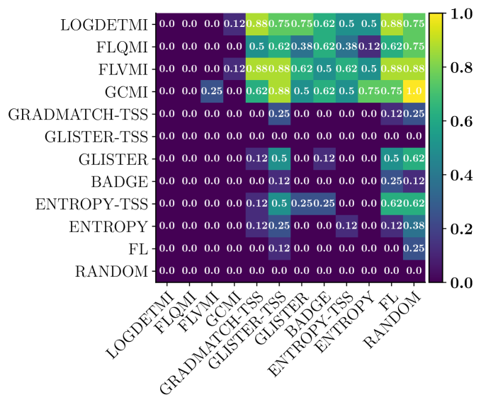
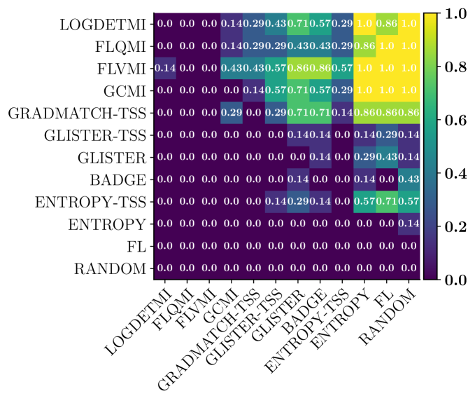
Figure 9: Penalty Matrix comparing the average accuracy of rare classes for MNIST (top) and SVHN (bottom) for different datasets using targeted learning across multiple budgets. We observe that the SMI functions have a much lower column sum compared to other approaches.

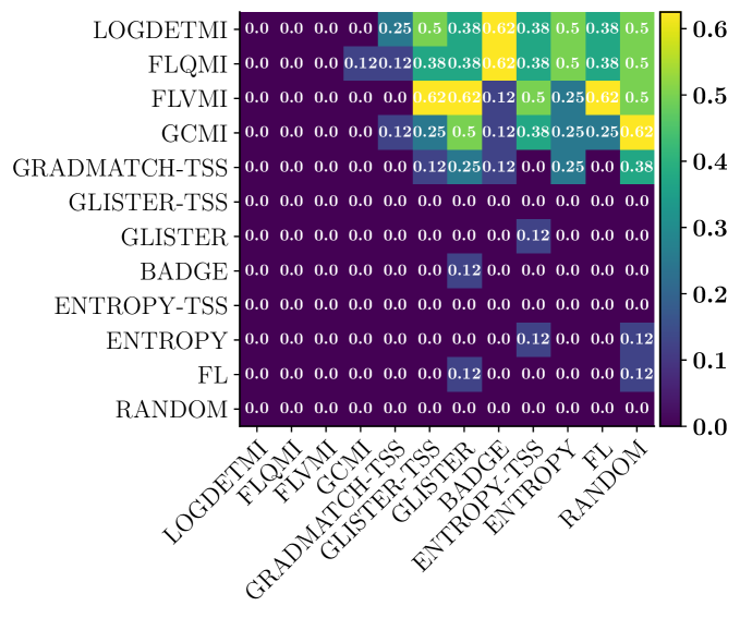
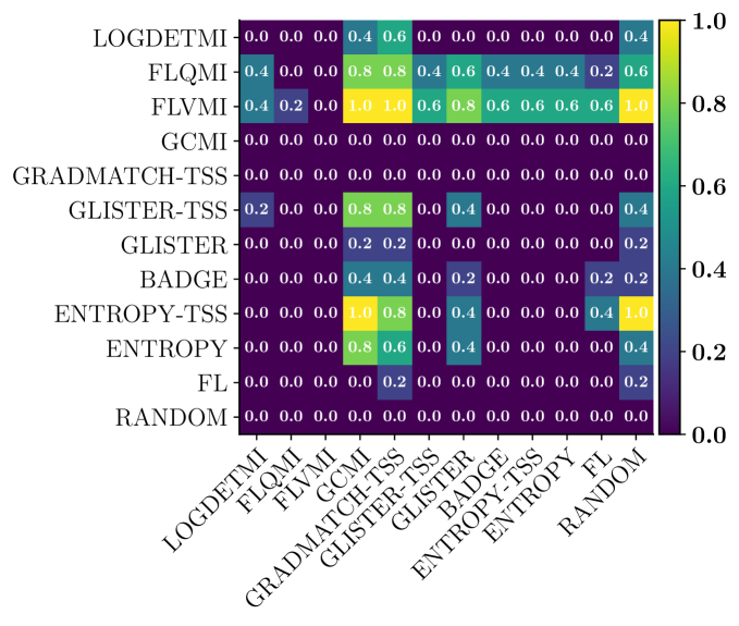
Figure 10: Penalty Matrix comparing the average accuracy of rare classes for CIFAR-10 (top) and Pneumonia-MNIST (bottom) for different datasets using targeted learning across multiple budgets. We observe that the SMI functions have a much lower column sum compared to other approaches.

H.3 Details on Computing Labeling Efficiency

The labeling efficiency is computed as the ratio of the minimum number of labeled training instances needed for an AL algorithm to reach a particular average rare class accuracy to the minimum number of labeled training instances needed by random sampling to reach that average rare class accuracy. Since most of the baselines are unable to reach each, the average rare class accuracy obtained by the MI functions at low budgets, we run targeted learning at the same intervals as shown in Fig. 3 until the full unlabeled dataset is selected. Across multiple test accuracies for all datasets, we observe $20\times-50\times$ labeling efficiency compared to random and $2\times-4\times$ compared to the existing approaches.

Appendix I Additional Details on Guided Summarization using Prism (Section  3.2)

We use the image collection dataset of (Tschiatschek et al. 2014). The dataset has 14 image collections with 100 images each and provides many ( 50-250) human summaries per collection. We extend it by creating dense noun concept annotations for every image to make it suitable for our task. We start by designing the universe of concepts based on the 600 object classes in OpenImagesv6 (Kuznetsova et al. 2018) and 365 scenes in Places365 (Zhou et al. 2014). We eliminate concepts common to both (for example, closet) to get a unified list of 959 concepts. To ease the annotation process we adopt pseudo-labelling followed by human correction. Specifically for every image we get the concept labels from a Yolov3 model pre-trained on OpenImagesv6 (for object concepts) and a ResNet50 model pre-trained on Place365 (for scene concepts). We then ask 5 human annotators to separately and individually correct the automatically generated labels (pseudo-labels). This is followed by finding a consensus over the set of concepts for each image to arrive at the final annotation concept vectors for each image. We have developed a Python GUI tool to ease this pseudo-label correction process, which we plan to release.

In addition to the already available generic human summaries, we augment the dataset with query-focused, privacy-preserving and joint query-focused and privacy-preserving summaries for each image collection. Specifically, we design 2 uni-concept and 2 bi-concept queries / private sets for each image collection to cover different cases like a) both concepts belonging to same image b) both concepts belonging to different images c) only one concept in the image collection. This is similar in spirit to (Sharghi, Laurel, and Gong 2017). We ask a group of 10 human annotators (different from those who annotated for concepts) to create a human summary (of 5 images) for each image collection and query and/or private pair. To ensure gold standard summaries, we followed this by a verification round. Specifically, we asked at least three annotators to accept/reject the summaries thus produced and we discarded those human summaries which were rejected by two or more such human annotators.

Instructions to participants for object and scene annotations and screen shot of the tool

: these are available in Annotation_Guidelines.docx attached with the supplementary material.

Hourly wage paid to participants and the total amount spent on participant compensation:

The entire effort of creating object and scene annotations along with producing the human summaries required about 170 man hours paid at the rate of Indian Rupees (INR) 700 per man hour and hence the total compensation provided was about INR 1,20,000. That is, approximately 1715 USD.

To instantiate the mixture model components, we represent images using the probabilistic feature vector taken from the output layer of YOLOv3 model (Redmon and Farhadi 2018) pre-trained on the open images dataset (Kuznetsova et al. 2018) and concatenate it with the probability vector of scenes from the output layer of  (Zhou et al. 2014) trained on the Places365 dataset (Zhou et al. 2017). The queries which are sets of concepts are mapped to a similar feature space as $k$-hot vectors ($k$ being the number of concepts in a query) to facilitate image-query similarity. Thus, both images and queries and/or elements in private set are represented using a $|\mathcal{C}|$-dimensional vector where $\mathcal{C}$ is the universe of concepts.

While more complex queries and methods of learning joint embedding between text and images could be employed, we chose simpler alternatives to stick to the main focus area of this work.

We initialize the parameters randomly and train the mixture model for 20 epochs. As in (Tschiatschek et al. 2014), we use 1 - V-ROUGE in the max-margin learning ( discussed in Section 5.2) and update parameters using Nesterov’s accelerated gradient descent.

References

- Ash et al. (2020) Ash, J. T.; Zhang, C.; Krishnamurthy, A.; Langford, J.; and Agarwal, A. 2020. Deep Batch Active Learning by Diverse, Uncertain Gradient Lower Bounds. In ICLR.
- Celis and Keswani (2020) Celis, L. E.; and Keswani, V. 2020. Implicit Diversity in Image Summarization. Proceedings of the ACM on Human-Computer Interaction, 4(CSCW2): 1–28.
- Chali, Tanvee, and Nayeem (2017) Chali, Y.; Tanvee, M.; and Nayeem, M. T. 2017. Towards abstractive multi-document summarization using submodular function-based framework, sentence compression and merging. In Proceedings of the Eighth International Joint Conference on Natural Language Processing (Volume 2: Short Papers), 418–424.
- Fujishige (2005) Fujishige, S. 2005. Submodular functions and optimization. Elsevier.
- Gupta and Levin (2020) Gupta, A.; and Levin, R. 2020. The Online Submodular Cover Problem. In ACM-SIAM Symposium on Discrete Algorithms.
- Gygli, Grabner, and Gool (2015) Gygli, M.; Grabner, H.; and Gool, L. 2015. Video summarization by learning submodular mixtures of objectives. 2015 IEEE Conference on Computer Vision and Pattern Recognition (CVPR), 3090–3098.
- He et al. (2016) He, K.; Zhang, X.; Ren, S.; and Sun, J. 2016. Deep residual learning for image recognition. In Proceedings of the IEEE conference on computer vision and pattern recognition, 770–778.
- Iyer et al. (2021) Iyer, R.; Khargoankar, N.; Bilmes, J.; and Asanani, H. 2021. Submodular combinatorial information measures with applications in machine learning. In Algorithmic Learning Theory, 722–754. PMLR.
- Ji et al. (2019) Ji, Z.; Xiong, K.; Pang, Y.; and Li, X. 2019. Video summarization with attention-based encoder-decoder networks. IEEE Transactions on Circuits and Systems for Video Technology.
- Jiang and Han (2019) Jiang, P.; and Han, Y. 2019. Hierarchical Variational Network for User-Diversified & Query-Focused Video Summarization. In Proceedings of the 2019 on International Conference on Multimedia Retrieval, 202–206.
- Kaushal et al. (2019a) Kaushal, V.; Iyer, R.; Kothawade, S.; Mahadev, R.; Doctor, K.; and Ramakrishnan, G. 2019a. Learning from less data: A unified data subset selection and active learning framework for computer vision. In 2019 IEEE Winter Conference on Applications of Computer Vision (WACV), 1289–1299. IEEE.
- Kaushal et al. (2019b) Kaushal, V.; Iyer, R.; Kothawade, S.; Subramanian, S.; and Ramakrishnan, G. 2019b. A Framework Towards Domain Specific Video Summarization. 2019 IEEE Winter Conference on Applications of Computer Vision (WACV), 666–675.
- Kaushal et al. (2019c) Kaushal, V.; Iyer, R. K.; Doctor, K.; Sahoo, A.; Dubal, P.; Kothawade, S.; Mahadev, R.; Dargan, K.; and Ramakrishnan, G. 2019c. Demystifying Multi-Faceted Video Summarization: Tradeoff Between Diversity, Representation, Coverage and Importance. 2019 IEEE Winter Conference on Applications of Computer Vision (WACV), 452–461.
- Kermany et al. (2018) Kermany, D. S.; Goldbaum, M.; Cai, W.; Valentim, C. C.; Liang, H.; Baxter, S. L.; McKeown, A.; Yang, G.; Wu, X.; Yan, F.; et al. 2018. Identifying medical diagnoses and treatable diseases by image-based deep learning. Cell, 172(5): 1122–1131.
- Killamsetty et al. (2021) Killamsetty, K.; Sivasubramanian, D.; Mirzasoleiman, B.; Ramakrishnan, G.; De, A.; and Iyer, R. 2021. GRAD-MATCH: A Gradient Matching Based Data Subset Selection for Efficient Learning. In ICML.
- Killamsetty et al. (2020) Killamsetty, K.; Sivasubramanian, D.; Ramakrishnan, G.; and Iyer, R. 2020. GLISTER: Generalization based Data Subset Selection for Efficient and Robust Learning. arXiv preprint arXiv:2012.10630.
- Kirchhoff and Bilmes (2014) Kirchhoff, K.; and Bilmes, J. 2014. Submodularity for Data Selection in Machine Translation. In Empirical Methods in Natural Language Processing (EMNLP).
- Krause and Golovin (2014) Krause, A.; and Golovin, D. 2014. Submodular function maximization.
- Krizhevsky, Hinton et al. (2009) Krizhevsky, A.; Hinton, G.; et al. 2009. Learning multiple layers of features from tiny images.
- Kuznetsova et al. (2018) Kuznetsova, A.; Rom, H.; Alldrin, N.; Uijlings, J.; Krasin, I.; Pont-Tuset, J.; Kamali, S.; Popov, S.; Malloci, M.; Duerig, T.; et al. 2018. The open images dataset v4: Unified image classification, object detection, and visual relationship detection at scale. arXiv preprint arXiv:1811.00982.
- LeCun et al. (1989) LeCun, Y.; Boser, B.; Denker, J. S.; Henderson, D.; Howard, R. E.; Hubbard, W.; and Jackel, L. D. 1989. Backpropagation applied to handwritten zip code recognition. Neural computation, 1(4): 541–551.
- LeCun et al. (1998) LeCun, Y.; Bottou, L.; Bengio, Y.; and Haffner, P. 1998. Gradient-based learning applied to document recognition. Proceedings of the IEEE, 86(11): 2278–2324.
- Li, Li, and Li (2012) Li, J.; Li, L.; and Li, T. 2012. Multi-document summarization via submodularity. Applied Intelligence, 37(3): 420–430.
- Lin (2012) Lin, H. 2012. Submodularity in natural language processing: algorithms and applications. Ph.D. thesis.
- Lin and Bilmes (2011) Lin, H.; and Bilmes, J. 2011. A class of submodular functions for document summarization. In Proceedings of the 49th Annual Meeting of the Association for Computational Linguistics: Human Language Technologies, 510–520.
- Lin and Bilmes (2012) Lin, H.; and Bilmes, J. A. 2012. Learning mixtures of submodular shells with application to document summarization. arXiv preprint arXiv:1210.4871.
- Mirzasoleiman et al. (2015) Mirzasoleiman, B.; Badanidiyuru, A.; Karbasi, A.; Vondrák, J.; and Krause, A. 2015. Lazier than lazy greedy. In Proceedings of the AAAI Conference on Artificial Intelligence, volume 29.
- Mirzasoleiman, Bilmes, and Leskovec (2020) Mirzasoleiman, B.; Bilmes, J.; and Leskovec, J. 2020. Coresets for data-efficient training of machine learning models. In International Conference on Machine Learning, 6950–6960. PMLR.
- Nemhauser, Wolsey, and Fisher (1978) Nemhauser, G. L.; Wolsey, L. A.; and Fisher, M. L. 1978. An analysis of approximations for maximizing submodular set functions—I. Mathematical programming, 14(1): 265–294.
- Netzer et al. (2011) Netzer, Y.; Wang, T.; Coates, A.; Bissacco, A.; Wu, B.; and Ng, A. Y. 2011. Reading digits in natural images with unsupervised feature learning.
- Ozkose et al. (2019) Ozkose, Y. E.; Celikkale, B.; Erdem, E.; and Erdem, A. 2019. Diverse Neural Photo Album Summarization. In 2019 Ninth International Conference on Image Processing Theory, Tools and Applications (IPTA), 1–6. IEEE.
- Redmon and Farhadi (2018) Redmon, J.; and Farhadi, A. 2018. Yolov3: An incremental improvement. arXiv preprint arXiv:1804.02767.
- Sener and Savarese (2018) Sener, O.; and Savarese, S. 2018. Active Learning for Convolutional Neural Networks: A Core-Set Approach. In International Conference on Learning Representations.
- Settles (2009) Settles, B. 2009. Active learning literature survey. Technical report, University of Wisconsin-Madison Department of Computer Sciences.
- Sharghi, Gong, and Shah (2016) Sharghi, A.; Gong, B.; and Shah, M. 2016. Query-focused extractive video summarization. In European Conference on Computer Vision, 3–19. Springer.
- Sharghi, Laurel, and Gong (2017) Sharghi, A.; Laurel, J. S.; and Gong, B. 2017. Query-focused video summarization: Dataset, evaluation, and a memory network based approach. In Proceedings of the IEEE Conference on Computer Vision and Pattern Recognition, 4788–4797.
- Singh, Virmani, and Subramanyam (2019) Singh, A.; Virmani, L.; and Subramanyam, A. 2019. Image Corpus Representative Summarization. In 2019 IEEE Fifth International Conference on Multimedia Big Data (BigMM), 21–29. IEEE.
- Tschiatschek et al. (2014) Tschiatschek, S.; Iyer, R. K.; Wei, H.; and Bilmes, J. A. 2014. Learning mixtures of submodular functions for image collection summarization. In Advances in neural information processing systems, 1413–1421.
- Vasudevan et al. (2017) Vasudevan, A. B.; Gygli, M.; Volokitin, A.; and Van Gool, L. 2017. Query-adaptive video summarization via quality-aware relevance estimation. In Proceedings of the 25th ACM international conference on Multimedia, 582–590.
- Wei, Iyer, and Bilmes (2015) Wei, K.; Iyer, R.; and Bilmes, J. 2015. Submodularity in data subset selection and active learning. In International Conference on Machine Learning, 1954–1963. PMLR.
- Xiao et al. (2020) Xiao, S.; Zhao, Z.; Zhang, Z.; Yan, X.; and Yang, M. 2020. Convolutional Hierarchical Attention Network for Query-Focused Video Summarization. In AAAI, 12426–12433.
- Yang, Shi, and Ni (2021) Yang, J.; Shi, R.; and Ni, B. 2021. Medmnist classification decathlon: A lightweight automl benchmark for medical image analysis. In 2021 IEEE 18th International Symposium on Biomedical Imaging (ISBI), 191–195. IEEE.
- Yao, Wan, and Xiao (2017) Yao, J.-g.; Wan, X.; and Xiao, J. 2017. Recent advances in document summarization. Knowledge and Information Systems, 53(2): 297–336.
- Zhou et al. (2017) Zhou, B.; Lapedriza, A.; Khosla, A.; Oliva, A.; and Torralba, A. 2017. Places: A 10 million Image Database for Scene Recognition. IEEE Transactions on Pattern Analysis and Machine Intelligence.
- Zhou et al. (2014) Zhou, B.; Lapedriza, A.; Xiao, J.; Torralba, A.; and Oliva, A. 2014. Learning deep features for scene recognition using places database. In Advances in neural information processing systems, 487–495.