Visualizing Music Genres using a Topic Model

Abstract

Music Genres serve as an important meta-data in the field of music information retrieval and have been widely used for music classification and analysis tasks. Visualizing these music genres can thus be helpful for music exploration, archival and recommendation. Probabilistic topic models have been very successful in modelling text documents. In this work, we visualize music genres using a probabilistic topic model. Unlike text documents, audio is continuous and needs to be sliced into smaller segments. We use simple MFCC features of these segments as musical words. We apply the topic model on the corpus and subsequently use the genre annotations of the data to interpret and visualize the latent space.

1 Introduction

It is suggested by [Wells(1992)] that musicologists identify music genres as pieces of music that have a similar musical language or structure. Music genre analysis tasks are widely pursued in the music information retrieval community. However, genre visualizations have not caught enough attention. Music Genre Visualization can be very helpful in modern technologies such as custom music playlists and recommendation systems. Probabilistic Topic Models [Blei(2012)], have found wide applications in the field of Natural Language processing. We use an unsupervised topic model on music genres data for visualization. For our work we use raw music files, in .wav format. Unlike text documents, raw music data has no discrete components such as words. To create a text-like corpus, we slice the audio data into smaller segments. We use MFCC features of these smaller slices as the representation. Further, to build a corpus, we create a feature dictionary by using the k-means algorithm. Also, in text documents, the inferred topics form a collection of words and hence are straightforward to interpret. In our case, musical words, which are mere MFCC feature arrays, lack inherent meaning and cannot be interpreted. We interpret the latent space of the topic model using genre annotations in the dataset.

2 Related Work

The work in [Cooper et al.(2006)Cooper, Foote, Pampalk, and Tzanetakis] presented a summary of and had discussed some audio visualization techniques in MIR which are mostly signal processing based. Topic Models have also been applied on audio in [Kim et al.(2012)Kim, Georgiou, and Narayanan] for audio classification and [Kim et al.(2009)Kim, Narayanan, and Sundaram] for audio information retrieval. The work in [Shalit et al.(2013)Shalit, Weinshall, and Chechik] uses a topic model to model musical influence. The work in [Hu and Saul()] applies a topic model on musical notes for key analysis.The work in [Hirai et al.(2016)Hirai, Doi, and Morishima] and [Hirai et al.(2018)Hirai, Doi, and Morishima] also use this models on music in the context of DJ performance. Similarly, the work in [Hariri et al.(2012)Hariri, Mobasher, and Burke] uses topic models on music tags for use in recommendation systems. We use the fault-filtered GTZAN [Tzanetakis and Cook(2002)] dataset for genre analysis which is popular in MIR community.

3 The Probabilistic Topic Model

Probabilistic topic models are based upon an idea that documents are mixture of topics and topics are probability distributions over words. These words come from a fixed size vocabulary. To make a new document, one chooses a distribution of topics, then chooses a topic from this distribution and finally draws a word from the chosen topic. The Latent Dirichlet Allocation (LDA) inverts this generative process and thus infers the set of topics that were that useful in generating the document. The plate notation also helps understand the generative process.

Using some mathematical notations, the generative process can be defined as follows. Let $K$ be the specified number of topics, $V$ the size of the vocabulary, $\alpha$ a positive $K$-vector and $\eta$ a scalar. Let ${Dir_{V}}$($\alpha$) denote a $V$-dimensional dirichlet with a vector parameter $\vec{\alpha}$ and Let ${Dir_{K}}$($\eta$) denote a K-dimensional dirichlet with a scalar parameter $\eta$.

1. For each topic

   • Draw a distribution over words $\beta_{K}$ over ${Dir_{V}}$($\eta$)

2. For each document

   • Draw a vector of topic proportions $\theta_{d}$ over $Dir{(\alpha)}$

   • For each word

     • Draw a topic assignment ${Z_{d,n}}$ over
       Mult(${\theta_{d}}$),${Z_{d,n}}$ $\epsilon$ ${1,2,...,K}$

     • Draw a word ${W_{d,n}}$ over
       Mult($\beta_{Z_{d,n}}$), ${W_{d,n}}$ $\epsilon$ ${1,2,...,V}$

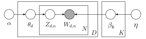
Figure 1: Plate Notation for a Topic Model

The above figure describes the generative process of the LDA algorithm using a what is called as a plate notation. The shaded variable ${W_{d,n}}$ is observable while all other variables are latent. The direction of the arrows help in understanding the generative process of the algorithm.

4 Applying Topic Models on Music

The main challenge with the application of topic models in the music (with raw audio files) is to represent the audio in a text-document like corpus. The intent of the work is to interpret the latent space of the topic model using music genres. This interpretation would help giving a probabilistic genre annotation to a song. For example a song may belong 60 % to Blues, 15 % to Jazz and 25 % to Pop genres. To enable such a probabilistic assignment, we build basic genre buckets consisting of at least 3 genres. We do this since a mixture containing all the 10 genres would be very large and obfuscating for the listener to meaningfully interpret. The rationale used to bucket the genres is roughly based on the histories and the musical form of these genres. The first bucket consists of Rock, Metal and Pop genres; the second of Blues, Jazz and Country genres and the final bucket consists of Reggae, Disco and Hip-Hop genres. The songs were clipped down to 0.10 seconds clips. The MFCC features of these clips were then calculated. We then use a K means clustering algorithm on the MFCC features to build the dictionary. It partitions the data into k clusters, where each data point belongs to a cluster and the cluster mean serves as its prototype. The librosa package [McFee et al.(2015)McFee, Raffel, Liang, Ellis, McVicar, Battenberg, and Nieto] was used for the computation and the pre-processing while the models are implemented using gensim package. An algorithmic description of the process is given as below.

1. For each song

   • Discretize into clips of 0.10 secs

   • Calculate MFCC features of these clips.

2. For all songs in a genre bucket

   • Calculate K-means (K=3) of the MFCC feature vectors

   • Map each MFCC feature vector (and thus the song) to any of the K-clusters

   • Apply the textual probabilistic topic model

5 Interpretation of the Latent Space

Unlike text documents, where topics are interpreted as a mixture of words; the acoustic topic model has topics which are mixtures of cluster means. These cluster means are prototypes of the nearest datapoints(the audiofiles) and thus lack meaning. It is thus essential to assign a suitable meaning to these cluster means. The first part of the interpretation involves understanding the cluster means in terms of music genre. The cluster means are constructed from the MFCC arrays. The cluster means hence can be mapped to and from these audio files and linked with the genre annotations. For instance, lets say that 3 audio files, audio1, audio4 and audio7 make up a cluster mean. We get back to the dataset and find out that audio1 belongs to the Blues genre, audio4 belongs to the Country genre and the audio7 belongs to the Blues genre. Hence, the genres associated with cluster means becomes Blues, Country,Blues. In math, the cluster centers (or terms) can be described as the following,

$$clustermean1 =\{Blues,Country,Blues\}$$ (1)

$$=0.67Blues+0.33Country$$

$$clustermean2 =\{Blues,Jazz,Jazz,Country\}$$

$$=0.25Blues+0.5Jazz+0.25Country$$

Once we interpret cluster means in terms of music genres, we can conveniently represent the topics in terms of music genres. The topic space consists of cluster means and an associated probability value. The cluster means can now be defined as music genres with their proportions.

$$\begin{split}Topic1&=prob1*clustermean1+prob2*clustermean2\\ &=(prob1*0.67+prob2*0.25)Blues+\\ &(prob1*0.33+prob2*0.25)Country\\ &+(prob2*0.5)Jazz\\ \end{split}$$ (2)

5.1 Document-Topic Proportions

Once the topic space has been interpreted, the document-topic proportions can also be made sense of. The document topic proportions from the topic model are probability values of the inferred topics present in each document. In this context, the document topic proportions can provide with the proportions of different music genres present within the musical document, that is, a song.

$$\begin{split}Doc1&=prob1*topic1+prob2*topic2\\ &=prob1*(0.33Blues+0.33Country+0.34Jazz)\\ &+prob2*(0.5Jazz+0.5Country)\\ &=(prob1*0.33)Blues+(prob1*0.34+prob2*0.5)Jazz\\ &+(prob1*0.33+prob2*0.5)Country\\ \end{split}$$ (3)

5.2 The Term-Topic Proportions

The term-topic proportions suggest the topic distributions in each term. So the term-topic distribution represents the genres present in each term, or cluster center. This is represented in an equation as,

$$\begin{split}Term1&=prob1*topic1+prob2*topic4\\ &=prob1*(0.33Blues+0.50Country+0.17Jazz)\\ &+prob2*(0.5Blues+0.5Jazz)\\ &=(prob1*0.33+prob2*0.5)Blues+(prob1*0.17+prob2*0.5)Jazz\\ &+(prob2*0.5)Country\\ \end{split}$$ (4)

The term-topic proportions is an interesting insight derived from the topic models. The terms are cluster centers derived from MFCC feature arrays. These feature arrays are in turn derived from small segments of a song. So the term-topic proportion suggest the genre proportions of each small segment of a song. For instance, 3 small segments of a song can belong to Blues-Classical, Jazz-Pop-Classical or Disco-Rock genres in some proportions.

6 Evaluating the Topic Model

We evaluate the model using a genre classification task. We use the model to get the document-topic proportions of every document(song). We use these document-topic proportions as a representation for each song. We use genre labels from the fault-filtered GTZAN dataset, divide the data into train-test sets and perform the classification task using a SVM. We also test our model with different number of topics to look for the optimal number of topics that best capture the genre bucket.

	2	3	4	5
1	0.47	0.53	0.58	0.53
2	0.36	0.38	0.35	0.40
3	0.53	0.46	0.48	0.50

Table 1: Accuracies obtained for different number of topic terms. The rows represent the genre bucket, while the columns represent the number of topics

7 Music Genre Visualization

Using the topic model, we can get a probabilistic genre labels of different songs(from document-topic proportions) along with progressive genre visualizations(from term-topic proportions).

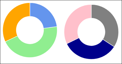
Figure 2: The above is a visualization of two topics emerging out of genre buckets 1 and 2 respectively. The colours represent the music genres and the doughnut partitions show genre proportions within a topic.

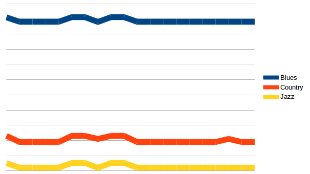
Figure 3: The progressive viz of a song segment. The x-axis denotes time and the y-axis the genre proportions. The above figure displays the changing genre proportions as the song progresses.

8 Conclusion

In this work, we applied a Probabilistic Topic Model on raw Music data and used the available genre annotations to interpret the latent space. We used the inferred parameters of the Topic Model to visualize the Music Data and also proposed some genre visualizations. Further, it would be interesting to explore other audio features and genre data for visualization using the Topic Model.

References

- [Blei(2012)] David M Blei. Probabilistic topic models. Communications of the ACM, 55(4):77–84, 2012.
- [Cooper et al.(2006)Cooper, Foote, Pampalk, and Tzanetakis] Matthew Cooper, Jonathan Foote, Elias Pampalk, and George Tzanetakis. Visualization in audio-based music information retrieval. Computer Music Journal, 30(2):42–62, 2006.
- [Hariri et al.(2012)Hariri, Mobasher, and Burke] Negar Hariri, Bamshad Mobasher, and Robin Burke. Context-aware music recommendation based on latenttopic sequential patterns. In Proceedings of the sixth ACM conference on Recommender systems, pages 131–138. ACM, 2012.
- [Hirai et al.(2016)Hirai, Doi, and Morishima] Tatsunori Hirai, Hironori Doi, and Shigeo Morishima. Musicmixer: Automatic dj system considering beat and latent topic similarity. In International Conference on Multimedia Modeling, pages 698–709. Springer, 2016.
- [Hirai et al.(2018)Hirai, Doi, and Morishima] Tatsunori Hirai, Hironori Doi, and Shigeo Morishima. Latent topic similarity for music retrieval and its application to a system that supports dj performance. Journal of Information Processing, 26:276–284, 2018.
- [Hu and Saul()] Diane J Hu and Lawrence K Saul. A probabilistic topic model for music analysis.
- [Kim et al.(2009)Kim, Narayanan, and Sundaram] Samuel Kim, Shrikanth Narayanan, and Shiva Sundaram. Acoustic topic model for audio information retrieval. In Applications of Signal Processing to Audio and Acoustics, 2009. WASPAA’09. IEEE Workshop on, pages 37–40. IEEE, 2009.
- [Kim et al.(2012)Kim, Georgiou, and Narayanan] Samuel Kim, Panayiotis Georgiou, and Shrikanth Narayanan. Latent acoustic topic models for unstructured audio classification. APSIPA Transactions on Signal and Information Processing, 1, 2012.
- [McFee et al.(2015)McFee, Raffel, Liang, Ellis, McVicar, Battenberg, and Nieto] Brian McFee, Colin Raffel, Dawen Liang, Daniel PW Ellis, Matt McVicar, Eric Battenberg, and Oriol Nieto. librosa: Audio and music signal analysis in python. In Proceedings of the 14th python in science conference, pages 18–25, 2015.
- [Shalit et al.(2013)Shalit, Weinshall, and Chechik] Uri Shalit, Daphna Weinshall, and Gal Chechik. Modeling musical influence with topic models. In International Conference on Machine Learning, pages 244–252, 2013.
- [Tzanetakis and Cook(2002)] George Tzanetakis and Perry Cook. Musical genre classification of audio signals. IEEE Transactions on speech and audio processing, 10(5):293–302, 2002.
- [Wells(1992)] Paul F Wells. Origins of the popular style: The antecedents of twentieth-century popular music, 1992.