Power series expansion neural network

Abstract

In this paper, we develop a new neural network family based on power series expansion, which is proved to achieve a better approximation accuracy in comparison with existing neural networks. This new set of neural networks embeds the power series expansion (PSE) into the neural network structure. Then it can improve the representation abilitiy while preserving comparable computational cost by increasing the degree of PSE instead of increasing the depth or width. Both theoretical approximation and numerical results show the advantages of this new neural network.

We develop a new set of neural network by introducing power series expansion;

Theoretical analysis shows that PSENet has a better approximation.

The new set of neural networks has been tested on different datasets and is shown the advantages;

1 Introduction

Machine learning has been experiencing an extraordinary resurgence in many important artificial intelligence applications since the late 2000s. In particular, it has produced state-of-the-art accuracy in computer vision, video analysis, natural language processing, and speech recognition. Recently, interest in machine learning-based approaches in the applied mathematics community has increased rapidly [18, 35, 38]. This growing enthusiasm for machine learning stems from a massive amount of data available from scientific computations and other sources: the design of efficient data analysis algorithms, advances in high-performance computing and the data-driven modeling [19, 21]. To date, there are also many theoretical works on the approximation rate of the neural network, such as cosine neural networks [17], sigmoidal neural networks[5], shallow ReLU^k networks [32], and Deep ReLU networks [20, 30]. However, the main challenge of machine learning is the training process as both complexity and memory requirements grow rapidly [6] for deep or wide neural networks. Thus this significant increase in computational cost may not be justified by the performance gain that approximation theories bring. Power Series Expansion (PSE) has been widely used in function approximation and the resulting linear system can be easily solved even for large-scale computation, for instance, spectral method [29]. However, the curse of dimensionality is the main obstacle in the numerical treatment of most high-dimensional problems based on the PSE approximation. In this paper, we will combine the ideas of neural network and PSE to develop a new network, which we call PSENet. This new network can achieve a higher accuracy even for shallow or narrow networks.

2 The formulation of PSENet

Feed-forward neural networks, consisting of a series of fully connected layers, can be written as a function from the input $x\in\mathbb{R}^{d}$ to the output $y\in\mathbb{R}^{\kappa}$. Mathematically, such a neural network with $L$ hidden layers can be written as follows

$$y(x;\theta)=W_{{\color[rgb]{0,0,0}L+1}}h_{L}+b_{L+1},~{}h_{i}=\sigma(W_{i}h_{i-1}+b_{i}),i\in\{1,\cdots,L\},\hbox{and }h_{0}=x,$$ (1)

where $W_{i}\in\mathbb{R}^{{\color[rgb]{0,0,0}d_{i}\times d_{i-1}}}$ is the weight matrix, $b_{i}\in\mathbb{R}^{{\color[rgb]{0,0,0}d_{i}}}$ is the bias, $d_{i}$ is the width of the $i$-th hidden layer ($d_{0}=d,d_{L+1}=\kappa$), and $\sigma$ is the activation function (for example, the rectified linear unit (ReLU) or the sigmoid activation functions) which is simply applied element-wise on each layer. Moreover, there is no activation function on the read-out layer since we consider the regression problems.

Inspired by the power series expansion for a smooth function $f(x)$, namely, $\displaystyle f(x)\approx\sum_{j=0}^{n}\alpha_{j}x^{j}$, we define each layer by analogy to a power series expansion. More precisely, we define a typical PSENet architecture as:

$$y(x;\theta)=W_{L+1}h_{L}+b_{L+1},~{}h_{i}=\sum_{j=0}^{n}{\alpha_{i,j}}\odot\sigma^{j}(W_{i}h_{i-1}+b_{i}),i\in\{1,\cdots,L\},\hbox{and }h_{0}=x,$$ (2)

where $\alpha_{i,j}\in\mathbb{R}^{d_{i}}$ are the unknown coefficients, $\alpha_{i,j}\odot\sigma^{j}(W_{i}h_{i-1}+b_{i})$ denoting the Hadamard product of vectors means element-wise multiplication and $\sigma^{j}$ stands for $j$-th power of the activation function. Specifically, we define $\sigma^{0}(x)=x$ as the identity function. Thus the PSENet is reduced to the ResNet by setting $n=1$ and $\alpha_{i,0}=\alpha_{i,1}=(1,1,\cdots,1)$:

$$h_{i}=\sigma(W_{i}h_{i-1}+b_{i})+{\color[rgb]{0,0,0}W_{i}h_{i-1}+b_{i}}.$$ (3)

Thus the PSENet can be thought of as adding a shortcut (when $\alpha_{i,0}\neq 0$) or a skip connection that allows information to flow, well just say, more easily from one layer to the next’s next layer, i.e., it bypasses data along with normal neural network flow from one layer to the next layer after the immediate next.

For the sake of brevity when discussing the approximation properties of the network in Section 3, we define the following general architecture of a hidden layer in PSENet

$$h_{i}=\sum_{j=0}^{n}\alpha_{i,j}{\color[rgb]{0,0,0}\odot}\sigma^{j}(W_{i,j}h_{i-1}+b_{i,j}),$$ (4)

where $W_{i,j}:\mathbb{R}^{d_{i}\times d_{i-1}}$ and $b_{i,j}\in\mathbb{R}^{d_{i}}$. On the one hand, it is easy to see that the original definition in (2) can be covered by the above formula if we make weights $W_{i,j}=W_{i}$ and $b_{i,j}=b_{i}$. On the other hand, one may imagine that the generalized PSENet in (4) can be reproduced by the PSENet defined in (2) by constructing a block-wise $W_{i}$ consisting of $(n-1)$ times replicates of $W_{i,j}$ and an appropriate $\alpha_{i,j}$ with a special sparse structure. As a consequence, we have the following theorem to show the equivalence between the two formulas.

Theorem 2.1.

Let $f(x):\mathbb{R}^{d}\mapsto\mathbb{R}^{\kappa}$ be a generalized PSENet model defined by (4) with hyper-parameters maximal power $n$ and widths $d_{i}$ for i=1:L. There exists a PSENet model $\tilde{f}(x)$ defined by (2) with hyper-parameters maximal power $n$ and widths $\tilde{d}_{i}={\color[rgb]{0,0,0}(n+1)}d_{i}$ for i=1:L, such that $\tilde{f}(x)=f(x)$.

Proof.

As defined in (4), the generalized PSENet function $f(x)$ has the form of $f(x)=W_{L+1}h_{L}(x)+b_{L}$ where

$$h_{i}(x)=\sum_{j=0}^{n}\alpha_{i,j}{\color[rgb]{0,0,0}\odot}\sigma^{j}(W_{i,j}h_{i-1}(x)+b_{i,j}),\quad i=1,\cdots,L,$$ (5)

where $h_{0}(x)=x$ and $W_{L+1}\in\mathbb{R}^{\kappa\times d_{L}}$. For simplicity, we denote $A_{i,j}={\rm Diag}(\alpha_{i,j})\in\mathbb{R}^{d_{i}\times d_{i}}$ as the diagonal matrix obtained by taking $\alpha_{i,j}$ as the diagonal elements. It follows that $\alpha_{i,j}{\color[rgb]{0,0,0}\odot}\sigma^{j}(W_{i,j}h_{i-1}(x)+b_{i,j})=A_{i,j}\sigma^{j}(W_{i,j}h_{i-1}(x)+b_{i,j})$ According to (2), we denote $\tilde{f}(x)=\tilde{W}_{L+1}\tilde{h}_{L}(x)+{\color[rgb]{0,0,0}\tilde{b}_{L+1}}$ where

$$\tilde{h}_{i}(x)=\sum_{j=0}^{n}\tilde{\alpha}_{i,j}{\color[rgb]{0,0,0}\odot}\sigma^{j}(\tilde{W}_{i}\tilde{h}_{i-1}(x)+\tilde{b}_{i}),\quad i=1,\cdots,L,$$ (6)

$\tilde{h}_{0}(x)=x$ and $\tilde{W}_{L+1}\in\mathbb{R}^{\kappa\times(n+1)d_{L}}$. Now, we construct $\tilde{f}(x)$ by taking

$$\tilde{W}_{i}=\begin{pmatrix}W_{i,0}A_{i-1,0}&W_{i,0}A_{i-1,1}&\cdots&W_{i,1}A_{i-1,n}\\ W_{i,1}A_{i-1,0}&W_{i,1}A_{i-1,1}&\cdots&W_{i,1}A_{i-1,n}\\ \vdots&\vdots&\vdots&\vdots\\ W_{i,n}A_{i-1,0}&W_{i,n}A_{i-1,1}&\cdots&W_{i,n}A_{i-1,n}\end{pmatrix}\in\mathbb{R}^{(n+1)d_{i}\times(n+1)d_{i-1}},\tilde{b}_{i}=\begin{pmatrix}b_{i,0}\\ b_{i,1}\\ \vdots\\ b_{i,n}\end{pmatrix}\in\mathbb{R}^{(n+1)d_{i}},$$ (7)

$$\text{ and }\tilde{\alpha}_{i,j}=\big{(}\underbrace{0,\cdots,0}_{(j-1)d_{i}},\underbrace{1,\cdots,1}_{d_{i}},\underbrace{0,\cdots,0}_{(n+1-j)d_{i}}\big{)}^{T}\in\mathbb{R}^{(n+1)d_{i}},$$ (8)

for $i=2,\cdots,L$. In addition, we take

$$\tilde{W}_{1}=\begin{pmatrix}W_{1,0}\\ W_{1,1}\\ \vdots\\ W_{1,n}\end{pmatrix},\tilde{b}_{1}=\begin{pmatrix}b_{1,0}\\ b_{1,1}\\ \vdots\\ b_{1,n}\end{pmatrix},\tilde{W}_{L+1}=\begin{pmatrix}W_{L+1}A_{L,0}\\ W_{L+1}A_{L,1}\\ \vdots\\ W_{L+1}A_{L,n}\end{pmatrix}^{T},\text{ and }\tilde{b}_{L+1}=b_{L+1}.$$ (9)

Then, we can finish the proof by showing that

$$\tilde{h}_{i}(x)=\begin{pmatrix}[\tilde{h}_{i}(x)]_{0}\\ [\tilde{h}_{i}(x)]_{1}\\ \vdots\\ [\tilde{h}_{i}(x)]_{n}\end{pmatrix}=\begin{pmatrix}\sigma^{1}(W_{i,0}h_{i-1}(x)+b_{i,0})\\ \sigma^{2}(W_{i,1}h_{i-1}(x)+b_{i,1})\\ \vdots\\ \sigma^{n}(W_{i,n}h_{i-1}(x)+b_{i,n})\end{pmatrix},$$ (10)

for $i=1,\cdots,L$. In fact, for $i=1$, we have

$$\tilde{h}_{1}(x)=\sum_{j=0}^{n}\tilde{\alpha}_{1,j}{\color[rgb]{0,0,0}\odot}\sigma^{j}(\tilde{W}_{1}x+\tilde{b}_{1})=\begin{pmatrix}\sigma^{1}(W_{1,0}x+b_{1,0})\\ \sigma^{2}(W_{1,1}x+b_{1,1})\\ \vdots\\ \sigma^{n}(W_{1,n}x+b_{1,n})\end{pmatrix}.$$ (11)

Then, by induction we have

$$\begin{aligned} &\tilde{h}_{i}(x)=\sum_{j=0}^{n}\tilde{\alpha}_{i,j}{\color[rgb]{0,0,0}\odot}\sigma^{j}(\tilde{W}_{i}\tilde{h}_{i-1}(x)+\tilde{b}_{i})=\begin{pmatrix}\sigma^{1}(W_{i,0}\sum_{j=0}^{n}A_{i-1,j}[\tilde{h}_{i-1}(x)]_{j}+b_{i,0})\\ \sigma^{2}(W_{i,1}\sum_{j=0}^{n}A_{i-1,j}[\tilde{h}_{i-1}(x)]_{j}+b_{i,1})\\ \vdots\\ \sigma^{n}(W_{i,n}\sum_{j=0}^{n}A_{i-1,j}[\tilde{h}_{i-1}(x)]_{j}+b_{i,n})\end{pmatrix}\\ &=\begin{pmatrix}\sigma^{1}\left(W_{i,0}\left(\sum_{j=0}^{n}A_{i-1,j}\sigma^{j}(W_{i-1,j}h_{i-2}(x)+b_{i-1,j})\right)+b_{i,0}\right)\\ \sigma^{2}\left(W_{i,1}\left(\sum_{j=0}^{n}A_{i-1,j}\sigma^{j}(W_{i-1,j}h_{i-2}(x)+b_{i-1,j})\right)+b_{i,1}\right)\\ \vdots\\ \sigma^{n}\left(W_{i,n}\left(\sum_{j=0}^{n}A_{i-1,j}\sigma^{j}(W_{i-1,j}h_{i-2}(x)+b_{i-1,j})\right)+b_{i,n}\right)\end{pmatrix}=\begin{pmatrix}\sigma^{1}(W_{i,0}h_{i-1}(x)+b_{i,0})\\ \sigma^{2}(W_{i,1}h_{i-1}(x)+b_{i,1})\\ \vdots\\ \sigma^{n}(W_{i,n}h_{i-1}(x)+b_{i,n})\end{pmatrix}\end{aligned}.$$ (12)

Therefore, we have

$$\tilde{f}(x)=\tilde{W}_{L+1}\tilde{h}_{L}(x)+{\color[rgb]{0,0,0}\tilde{b}_{L+1}}=W_{L+1}\sum_{j=0}^{n}\alpha_{L,j}{\color[rgb]{0,0,0}\odot}\sigma^{j}(W_{L,j}h_{L-1}(x)+b_{L,j})+{\color[rgb]{0,0,0}b_{L+1}}=W_{L+1}h_{L}(x)+{\color[rgb]{0,0,0}b_{L+1}}=f(x),$$ (13)

which finishes the proof. ∎

3 Representation abilities and approximation properties of PSENet

In this section, we will discuss the representation abilities and approximation power of PSENet defined in (4) in comparison with classical DNN under the ReLU activation function, ${\rm ReLU}(x)$, i.e.

$$\sigma(x)={\rm ReLU}(x):=\max\{0,x\},\quad x\in\mathbb{R}.$$

3.1 One-hidden-layer PSENet

Given Theorem 2.1, we consider a typical generalized PSENet function (i.e. $\kappa=1$) as

$$f(x)=W_{2}\left(\sum_{j=0}^{n}\alpha_{1,j}\odot\sigma^{j}(W_{1,j}x+b_{1,j})\right).$$

Since $W_{2}\in\mathbb{R}^{1\times d_{i}}$, we can merge $W_{1}$ and $\alpha_{1,j}$ and rewrite $f(x)$ as

$$f(x)=\sum_{j=0}^{n}\bar{\alpha}_{1,j}\sigma^{j}(W_{1,j}x+b_{1,j}),$$

where $\bar{\alpha}_{1,j}\in\mathbb{R}^{1\times d_{1}}$ and $\bar{\alpha}_{1,j}\sigma^{j}(W_{1,j}x+b_{1,j})$ is defined by standard matrix multiplication. Then, we may further generalize the above equation by taking $W_{1,j}\in\mathbb{R}^{m_{j}\times d}$ for $j=0,\cdots,n$ and for any $(m_{0},m_{1},\cdots,m_{n})\in\mathbb{N}^{n}$. Then we denote the set of generalized one-hidden-layer PSENet function as

$$V_{\bm{m}}^{n}=\left\{f(x)=\sum_{j=0}^{n}\alpha_{j}\sigma^{j}(W_{j}x+b_{j})~{}:~{}W_{j}\in\mathbb{R}^{m_{j}\times d},b_{j}\in\mathbb{R}^{m_{j}},\alpha_{j}\in\mathbb{R}^{1\times m_{j}}\right\},$$ (14)

for any $\bm{m}=(m_{0},m_{1},\cdots,m_{n})\in\mathbb{N}^{n}$. Here we notice that there exist $\omega\in\mathbb{R}^{d}$ and $b\in\mathbb{R}$ such that $\alpha_{0}\sigma^{0}(W_{0}x+b_{0})=\omega\cdot x+b$ is only a linear function on $\mathbb{R}^{d}$ no matter how big $m_{0}$ is. Thus, we always assume $m_{0}=1$ in $V_{\bm{m}}^{n}$.

Next we show the representation abilities and approximation power in terms of the largest power $n$ and the number of neurons $\displaystyle|\bm{m}|=\sum_{j=0}^{n}m_{j}$. Since the activation function and its powers are ${\rm ReLU}^{k}$, it is natural to consider the connections between the PSENet $V_{\bm{m}}^{n}$ and the B-Spline function space on one-dimensional space. According to [8], a one-dimensional cardinal B-Spline of degree $n\geq 0$ denoted by $b^{n}(x)$ for $x\in\mathbb{R}$, can be written as

$$b^{n}(x)=(n+1)\sum_{i=0}^{n+1}w_{i}\sigma^{n}(i-x)\text{~{}and~{}}w_{i}={\displaystyle\prod_{j=0,j\neq i}^{n+1}}\frac{1}{i-j},$$ (15)

where $b^{n}(x)$ is supported on $x\in[0,n+1]\subset\mathbb{R}$ and $n\geq 1$. Moreover, the cardinal B-Spline series of degree $n$ on the uniform grid with mesh size $h=\frac{1}{k+1}$ is defined as

$$B_{k}^{n}=\Big{\{}v(x)=\sum_{j=-n}^{k}c_{j}b^{n}_{j,h}(x)\Big{\}}\hbox{~{}where~{}}b^{n}_{j,h}(x)=b^{n}(\frac{x}{h}-j).$$ (16)

Then we have the following lemma for the representation abilities of $V_{\bm{m}}^{n}$ in terms of its connections with B-Spline function space.

Lemma 3.1.

By choosing $m_{i}\geq k_{i}+i+1$ ($i=1,\cdots,n$), we have

$$\bigcup_{i=1}^{n}B_{k_{i}}^{i}\subset V_{\bm{m}}^{n},$$ (17)

where $V_{\bm{m}}^{n}$ and $B_{k_{i}}^{i}$ are defined by (14) and (16), respectively.

Proof.

We consider the so-called finite neuron methods [36] with ${\rm ReLU}^{k}$ as the activation function and define the one hidden layer neural network described in [36] as

$${V}_{m}^{n}:=\left\{f(x)~{}:~{}f(x)=\sum_{j=1}^{m}a_{j}\sigma^{n}(\omega_{j}\cdot x+b_{j})\right\}.$$ (18)

Obviously, we have

$$V_{\bm{m}}^{n}=\bigcup_{i=0}^{n}V_{m_{i}}^{i}.$$ (19)

Lemma 3.2 in [36] shows that

$$B_{m}^{i}\subset{V}_{m+i+1}^{i},$$ (20)

then we complete the proof by combining (19) and (20). ∎

As a result of the above lemma, we have the following approximation result for $V_{\bm{m}}^{n}$.

Theorem 3.1 (1D case).

Suppose $u\in H^{n+1}(\Omega)$ for a bounded domain $\Omega\subset\mathbb{R}$, we have

$$\inf_{v\in V_{\bm{m}}^{n}}\|u-v\|_{s,\Omega}\lesssim\min_{i=1,2,\cdots,n}\left\{m_{i}^{s-(i+1)}\|u\|_{i+1,\Omega}\right\},$$ (21)

for any large enough $m_{i}>i+1$. Here $H^{k}(\Omega)$ (or $W^{k,2}(\Omega)$) denotes the standard Sobolev space [1] on $\Omega$ with norm $\|u\|_{k,\Omega}$.

Proof.

According to the error estimate of $B^{i}_{N}$ in [36], we have

$$\inf_{v\in B_{m_{i}-i-1}^{i}}\|u-v\|_{s,\Omega}\lesssim m_{i}^{s-(i+1)}\|u\|_{i+1,\Omega}.$$ (22)

In addition, we have

$$\bigcup_{i=1}^{n}B_{m_{i}-i-1}^{i}\subset V_{\bm{m}}^{n},$$ (23)

if $m_{i}>i+1$ in Lemma 3.1. This indicates that

$$\inf_{v\in V_{\bm{m}}^{n}}\|u-v\|_{s,\Omega}\leq\inf_{v\in\cup_{i=1}^{n}B_{m_{i}-i-1}^{i}}\|u-v\|_{s,\Omega}\lesssim\min_{i=1,2,\cdots,n}\left\{m_{i}^{s-(i+1)}\|u\|_{i+1,\Omega}\right\}.$$ (24)

∎

Remark 3.1.

When comparing with ${\rm ReLU}^{n}$-DNN  [36], the PSENet has the following advantages:

1. If we have no information about the regularity of the target function $u(x)$ a priori, the PSENet $V_{\bm{m}}^{n}$ gives an adaptive and uniform scheme for approximating any $u\in H^{i}(\Omega)$ for all $i\geq 1$. However, ${\rm ReLU}^{n}$-DNN can only work for $u\in H^{i}(\Omega)$ for $i\geq n$.

2. By choosing $m_{i}=0$ for $i<n$, the PSENet $V_{\bm{m}}^{n}$ recovers the ${\rm ReLU}^{n}$-DNN exactly. Thus if $u(x)\in H^{n}(\Omega)$, then PSENet provides almost the same asymptotic convergence rate in terms of the number of hidden neurons $|\bm{m}|$ as the ${\rm ReLU}^{n}$-DNN  [36].

3. If $u(x)$ is a smooth function, the PSENet $V_{\bm{m}}^{n}$ then provides a better approximation than ${\rm ReLU}^{n}$-DNN when the number of neurons, $m$, is not large since $\|u\|_{i+1,\Omega}$ might be very large but $\left(\frac{|\bm{m}|}{n}\right)^{s-(i+1)}$ is not small enough.

Following the observation of Lemma (3.10) in [36], we have the next theorem about the representation abilities of the PSENet in terms of its connections with polynomials on the multi-dimensional space.

Theorem 3.2 (Multi-dimensional case).

For any polynomial $p(\bm{x})=\displaystyle\sum_{|\alpha|\leq k}a_{\alpha}\bm{x}^{\alpha}$ on $\mathbb{R}^{d}$, there exists a PSENet function $\hat{p}(x)=\displaystyle\sum_{j=0}^{k}c_{j}\sigma^{j}(W_{j}x+b_{j})$ with $m_{i}\leq 2\binom{i+d-1}{i}$, such that

$$\hat{p}(x)=p(x),$$ (25)

on $\mathbb{R}^{d}$.

Proof.

Given the connections between PSENet and $ReLU^{k}$-DNN in (19), we only need to prove

$$\left\{\sum_{|\alpha|=i}a_{\alpha}\bm{x}^{\alpha}~{}:~{}a_{\alpha}\in\mathbb{R}\right\}\subset V_{m_{i}}^{i}\hbox{~{}and~{}}m_{i}=2\binom{i+d-1}{i}.$$

To prove that, we first recall the following property that

$$x^{i}={\rm ReLU}^{i}(x)+(-1)^{i}{\rm ReLU}^{i}(-x).$$ (26)

Moreover $d_{i}=\binom{i+d-1}{i}$ is the dimension of the space of homogeneous polynomials on $\mathbb{R}^{d}$ with degree $i$. Thus, we only need to prove that we can choose suitable $w_{s}\in\mathbb{R}^{d}$ for $s=1:d_{i}$ such that

$$(w_{s}\cdot\bm{x})^{i}={\rm ReLU}^{i}(w_{s}\cdot x)+(-1)^{i}{\rm ReLU}^{i}(-w_{s}\cdot x)\in\text{PSENet},$$ (27)

forms a basis for homogeneous polynomials on $\mathbb{R}^{d}$ with degree $i$. By denoting

$$\bm{X}=(\bm{x}^{\alpha_{1}},\bm{x}^{\alpha_{2}},\cdots,\bm{x}^{\alpha_{d_{i}}})^{T},$$ (28)

as the natural basis for the space of homogeneous polynomials on $\mathbb{R}^{d}$ with degree $i$, we have

$$((w_{1}\cdot\bm{x})^{i},(w_{2}\cdot\bm{x})^{i},\cdots,(w_{d_{i}}\cdot\bm{x})^{i})^{T}=\bm{W}\bm{X},$$ (29)

where $\bm{W}\in\mathbb{R}^{d_{i}\times d_{i}}$ is a matrix formed by $w_{1},w_{2},\cdots,w_{d_{i}}$. Based on the generalized Vandermonde determinant identity [37], we see that $\bm{W}$ is an invertible matrix if we choose appropriate $w_{s}$. Therefore $((w_{1}\cdot\bm{x})^{i},(w_{2}\cdot\bm{x})^{i},\cdots,(w_{d_{i}}\cdot\bm{x})^{i})$ forms the basis for the space of homogeneous polynomials on $\mathbb{R}^{d}$ with degree $i$. A more comprehensive description about how to choose $w_{s}$ to get an invertible $\bm{W}$ will be available in [13]. ∎

Remark 3.2.

1. The total number of neurons is

   $$|\bm{m}|=\sum_{i=0}^{k}m_{i}=\sum_{i=0}^{k}2\binom{i+d-1}{i}=2\binom{k+d}{k},$$

   which equals the number of neurons of ${\rm ReLU}^{k}$-DNN to recover polynomials with degree $k$ as shown in [36]. Considering the spectral accuracy of polynomials for smooth functions in terms of the degree $k$, the above representation theorem shows that PSENet can achieve an exponential approximation rate for smooth functions with respect to $n$ in $V_{\bm{m}}^{n}$, some similar results can be found in [9, 12, 25, 26, 33]

2. PSENet can take a large degree $n$ to reproduce high order polynomials instead of a deep network. But other networks need deep layers to improve the performance, for example expressive power [2, 14, 15, 24, 31, 34], approximation properties [9, 10, 22, 23, 25, 26, 27], benefits for training [3] and etc.

3. The main results in this subsection are established by combining the representation abilities of the ${\rm ReLU}^{k}$-DNN $V^{k}_{m}$, i.e., its connection with B-Spline (Lemma 3.2 in [36]) and polynomials (Lemma 3.10 in [36]). Moreover, we also reveal the natural relation between the PSENet $V^{n}_{\bm{m}}$ and the ${\rm ReLU}^{k}$-DNN $V^{k}_{m}$ in (19). In the following subsection, we show another core feature of the PSENet $V^{n}_{\bm{m}}$ that it can approximate singular function with optimal rate. This has not been studied in [36], and the PSENet can achieve a better approximation rate compared to the results presented in both  [12] and [25].

3.2 Optimal approximation rate on singular functions by using PSENet

We apply the PSENet on the singular function approximation which has been widely studied in hp-FEM [4, 28] and consider non-smooth functions in Gevrey class [7, 28, 25] on $I=(0,1)$: For any $\beta>0$, we define the function $\varphi_{\beta}(x)=x^{\beta}$ on $[0,1]$, the seminorm as

$$|u|_{H_{\beta}^{k,\ell}(I)}:=||\varphi_{\beta+k-\ell}D^{k}u||_{L^{2}(I)},$$ (30)

and the $H^{k,\ell}_{\beta}$ norm as

$$||u||^{2}_{H_{\beta}^{k,\ell}(I)}:=\left\{\begin{split}&\sum\limits_{k^{\prime}=0}^{k}|u|^{2}_{H_{\beta}^{k^{\prime},0}(I)},&if~{}\ell=0,\\ &\sum\limits_{k^{\prime}=l}^{k}|u|^{2}_{H_{\beta}^{k^{\prime},\ell}(I)}+||u||^{2}_{H^{\ell-1}(I)},&if~{}\ell\geq 1,\end{split}\right.$$ (31)

where $\ell,k=0,1,2,\cdots$. For any $\delta\geq 1$ the Gevrey class $\mathcal{G}_{\beta}^{\ell,\delta}(I)$ is defined as the class of functions $u\in\cap_{k\geq l}H_{\beta}^{k,l}(I)$ for which there exist $M,m>0$, such that

$$\forall k\geq l:|u|_{H_{\beta}^{k,l}(I)}\leq Mm^{k-l}((k-l)!)^{\delta}.$$ (32)

When $d=1$, these function classes have a singular point at $x=0$, then the $hp$ finite element method has exponential convergence to this function class [28, 11].

We consider the piece-wise polynomial space on mesh $\mathcal{T}_{n}:0=x_{0}<\cdots<x_{n}=1$ as

$$\begin{split}P_{\bm{p}}(\mathcal{T}_{n})=\{p_{h}\mbox{ is continuous on }I~{}|~{}p_{h}\mbox{ is a polynomial on grid }[x_{i-1},x_{i}]\mbox{ with degree }p^{(i)}\},\end{split}$$ (33)

and have the following estimate:

Lemma 3.2 ([25]).

Let $\sigma,\beta\in(0,1),\delta\geq 1,u\in\mathcal{G}_{\beta}^{2,\delta}(I)$ and $N\in\mathbb{N}$ be given. For $\mu_{0}=\mu_{0}(\sigma,\delta,m):=\max\{1,\frac{m}{2}(2e)^{1-\delta}\}$ and for any $\mu>\mu_{0}$, let $\bm{p}=(p^{(i)})_{i=1}^{n}\subset\mathbb{N}$ be defined as $p^{(1)}:=1$ and $p^{(i)}:=\lfloor\mu i^{\delta}\rfloor$ for $i\in\{2,...,n\}$. Then there exists $v(x)\in P_{\bm{p}}(\mathcal{T}_{n})$ with $v(x_{i})=u(x_{i})$ and $x_{i}=\frac{1}{2^{n-i}}$ for $i\in\{1,...,n\}$ such that for constants $C(\sigma,\beta,\delta,\mu,M,m),c(\beta,\delta)>0$ it holds that

$$||u-v||_{H^{1}(0,1)}\leq Ce^{-cn}.$$ (34)

Then we have the following lemma about the decomposition properties of functions of PSENet in $P_{\bm{p}}(\mathcal{T}_{n})$ with $p^{(i)}\leq p^{(i+1)}$.

Lemma 3.3.

For any function $p_{h}\in P_{\bm{p}}(\mathcal{T}_{n})$ with $p^{(i)}\leq p^{(i+1)}$, $p_{h}(x)$ can be reproduced by a one-hidden-layer PSENet, namely,

$$p_{h}(x)=\sum_{j=0}^{p^{(n)}}\alpha_{j}\sigma^{j}(W_{j}x+b_{j}),\quad\forall x\in[0,1]$$ (35)

where $m_{j}\leq n$.

Proof.

First, we can write $p_{h}(x)$ as

$$p_{h}(x)-p_{h}(0)=\sum_{i=1}^{n}\chi_{I_{i}}(x)p_{h,i}(x),$$ (36)

where $\chi_{I_{i}}(x)$ is the indicator function of $I_{i}=[x_{i-1},x_{i})$ for $i=1,\cdots,n-1$, and $I_{n}=[x_{n-1},x_{n}]$. Here $p_{h,i}(x)$ is the polynomial of $p_{h}(x)$ on $I_{i}$ with degree $p^{(i)}$. Thanks to the property that $p^{(i)}\leq p^{(i+1)}$, we re-write $p_{h}(x)$ as

$$p_{h}(x)-p_{h}(0)=\sum_{i=1}^{n}\chi_{\tilde{I}_{i}}(x)\tilde{p}_{h,i}(x),$$ (37)

where $\tilde{I}_{i}=[x_{i-1},1]$ and $\tilde{p}_{h,i}(x)$ is a polynomial of degree $p^{(i)}$ defined as

$$\tilde{p}_{h,i}(x)=p_{h,i}(x)-\tilde{p}_{h,i-1}(x),\quad i=2,3,\cdots,n,$$ (38)

with $\tilde{p}_{h,1}(x)=p_{h,1}(x)$. In addition, we have

$$\tilde{p}_{h,i}(x)=\sum_{j=1}^{p^{(i)}}\tilde{a}^{(i)}_{j}(x-x_{i-1})^{j},$$ (39)

because of the continuity of $p_{h}(x)$ on $[0,1]$. Based on the above property and definition of indicator function $\chi_{\tilde{I}_{i}}(x)$, we have

$$\chi_{\tilde{I}_{i}}(x)\tilde{p}_{h,i}(x)=\sum_{j=1}^{p^{(i)}}\tilde{a}^{(i)}_{j}\sigma^{j}(x-x_{i-1}),$$ (40)

on $[0,1]$. That finishes the proof. ∎

This lemma is different from results in [25, 36, 12] since it can achieve an exact representation formula for any piecewise polynomials while their results can only construct the representation globally or establish some approximation results for the piecewise case.

Based on these two lemmas, we have the following main theorem for approximation property of PSENet for Gevrey class.

Theorem 3.3.

For all $\delta\geq 1$, $\beta\in(0,1)$, and $u\in\mathcal{G}_{\beta}^{2,\delta}(I)$, there exists a PSENet function $\hat{u}(x)$ with one hidden layer such that

$$||u-\hat{u}||_{H^{1}(0,1)}\leq C_{0}e^{-C_{1}|\bm{m}|^{\frac{1}{\delta+1}}},$$ (41)

where $\displaystyle|\bm{m}|=\sum_{j=0}^{p^{(n)}}m_{j}$ for $\hat{u}(x)$, and $C_{0}(\sigma,\beta,\delta,\mu,M,m)$ and $C_{1}(\beta,\delta)$ only depend on the function $u(x)$ , similar to Lemma 3.2.

Proof.

For any function $u(x)\in\mathcal{G}_{\beta}^{2,\delta}(I)$, Lemma 3.2 shows that there exists $u_{h}(x)\in P_{\bm{p}}(\mathcal{T}_{n})$ such that

$$||u-u_{h}||_{H^{1}(0,1)}\leq Ce^{-cn},$$ (42)

with $p^{(1)}:=1$ and $p^{(i)}:=\lfloor\mu i^{\delta}\rfloor$ for $i\in\{2,...,n\}$. According to Lemma 3.3, there exists a PSENet function $\hat{u}(x)$ with one hidden layer and $m_{j}\leq p^{(n)}-j+1$ such that $\hat{u}(x)=u_{h}(x)$ on $[0,1]$, i.e.

$$\|u-\hat{u}\|_{H^{1}(0,1)}=\|u-u_{h}\|_{H^{1}(0,1)}\leq Ce^{-cn}.$$ (43)

Then, it is easy to obtain the final approximation rate since

$$|\bm{m}|=\sum_{j=0}^{p^{(n)}}m_{j}\lesssim\mu n^{\delta+1}.$$ (44)

∎

This approximation result achieves a better convergence rate in comparison with results in [12] and  [25], whose rates are $C_{0}e^{-C_{1}M^{\frac{1}{2\delta+1}}}$ or $C_{0}e^{-C_{1}M^{\frac{1}{3\delta+1}}}$, respectively. Furthermore, this result is optimal since it shares the same order with the most general approximation result of piecewise polynomials.

4 Numerical results

In this section, we compare the PSENet with ResNet on both fully connected and convolutional neural networks by using the ReLU activation function.

4.1 Function approximation

We first compare the PSENet with fully connected neural networks and ResNet to approximate $y=sin(n\pi x)$ on $[0,1]$ and $y=\sin(n\pi(x_{1}+x_{2}))$ on $[0,1]\times[0,1]$ with single, two and three hidden layers. We train the neural networks with uniform grid points with a $0.01$ mesh size for both functions and use Adam training algorithm with a fixed learning rate $0.01$. The training loss for different neural networks are compared and shown in Table 4.1 which demonstrates that PSENet has a better approximation ability in comparison with the other two networks with the optimal degree shown . Secondly, we consider a 1D function $f(x)=x^{\alpha}$ with $\alpha\in(0,1)$ on $x\in[0,1]$, where $x=0$ is a singularity. From the theoretical analysis in Section 3.2, the PSENet can achieve a better approximation rate when compared to ReLU^k-DNN which is confirmed in Table 2.

Table 1: The comparison between PSENet and fully connected neural networks and ResNet on the training loss of $f(x)=\sin(n\pi x)$ on [0,1] and $y=\sin(n\pi(x_{1}+x_{2}))$ on $[0,1]\times[0,1]$. The number of neurons on each layer is 10. The best approximation accuracy for PSENet with different degree $n$ is highlighted.

	Function	FC	ResNet	PSENet
				n=1	n=2	n=3	n=4	n=5
1-hidden-layer	$\sin(3\pi x)$	$2\times 10^{-1}$	$2\times 10^{-1}$	$2\times 10^{-1}$	$1\times 10^{-1}$	$2\times 10^{-1}$	$1\times 10^{-1}$	$\bm{6\times 10^{-3}}$
	$\sin(4\pi x)$	$3\times 10^{-1}$	$2\times 10^{-1}$	$3\times 10^{-1}$	$4\times 10^{-1}$	$2\times 10^{-1}$	$\bm{1\times 10^{-1}}$	$2\times 10^{-1}$
	$\sin(5\pi x)$	$2\times 10^{-1}$	$3\times 10^{-1}$	$2\times 10^{-1}$	$2\times 10^{-1}$	$3\times 10^{-1}$	$1\times 10^{-1}$	$\bm{5\times 10^{-2}}$
2-hidden-layer	$\sin(3\pi x)$	$3\times 10^{-3}$	$4\times 10^{-3}$	$3\times 10^{-3}$	$2\times 10^{-1}$	$\bm{2\times 10^{-3}}$	$4\times 10^{-3}$	$3\times 10^{-3}$
	$\sin(4\pi x)$	$2\times 10^{-1}$	$3\times 10^{-1}$	$2\times 10^{-1}$	$3\times 10^{-1}$	$1\times 10^{-2}$	$\bm{3\times 10^{-4}}$	$2\times 10^{-2}$
	$\sin(5\pi x)$	$2\times 10^{-1}$	$1\times 10^{-1}$	$1\times 10^{-1}$	$1\times 10^{-1}$	$1\times 10^{-1}$	$3\times 10^{-1}$	$\bm{4\times 10^{-3}}$
3-hidden-layer	$\sin(3\pi x)$	$2\times 10^{-1}$	$1\times 10^{-3}$	$3\times 10^{-3}$	$1\times 10^{-3}$	$3\times 10^{-3}$	$8\times 10^{-4}$	$\bm{6\times 10^{-4}}$
	$\sin(4\pi x)$	$3\times 10^{-1}$	$3\times 10^{-1}$	$2\times 10^{-1}$	$3\times 10^{-1}$	$\bm{1\times 10^{-2}}$	$2\times 10^{-1}$	$1\times 10^{-1}$
	$\sin(5\pi x)$	$3\times 10^{-1}$	$1\times 10^{-1}$	$3\times 10^{-1}$	$1\times 10^{-1}$	$\bm{3\times 10^{-3}}$	$1\times 10^{-1}$	$1\times 10^{-1}$
2-hidden-layer	$\sin(3\pi(x_{1}+x_{2}))$	$2\times 10^{-1}$	$7\times 10^{-2}$	$2\times 10^{-2}$	$1\times 10^{-2}$	$6\times 10^{-3}$	$7\times 10^{-2}$	$5\times 10^{-2}$
	$\sin(4\pi(x_{1}+x_{2}))$	$4\times 10^{-1}$	$1\times 10^{-1}$	$2\times 10^{-1}$	$5\times 10^{-2}$	$4\times 10^{-1}$	$\bm{1\times 10^{-2}}$	$4\times 10^{-1}$
	$\sin(5\pi(x_{1}+x_{2}))$	$3\times 10^{-1}$	$4\times 10^{-1}$	$4\times 10^{-1}$	$4\times 10^{-1}$	$4\times 10^{-1}$	$4\times 10^{-1}$	$2\times 10^{-1}$
3-hidden-layer	$\sin(3\pi(x_{1}+x_{2}))$	$1\times 10^{-1}$	$1\times 10^{-1}$	$1\times 10^{-1}$	$\bm{2\times 10^{-3}}$	$2\times 10^{-2}$	$8\times 10^{-3}$	$1\times 10^{-2}$
	$\sin(4\pi(x_{1}+x_{2}))$	$3\times 10^{-1}$	$1\times 10^{-1}$	$1\times 10^{-1}$	$8\times 10^{-2}$	$\bm{7\times 10^{-2}}$	$1\times 10^{-1}$	$1\times 10^{-1}$
	$\sin(5\pi(x_{1}+x_{2}))$	$3\times 10^{-1}$	$4\times 10^{-1}$	$4\times 10^{-1}$	$3\times 10^{-1}$	$3\times 10^{-1}$	$3\times 10^{-1}$	$5\times 10^{-2}$

$\alpha$	ResNet	$ReLU^{k}$ Network					PSENet
		k=1	k=2	k=3	k=4	k=5	n=1	n=2	n=3	n=4	n=5
$2/3$	$3.6\times 10^{-2}$	$3.0\times 10^{-2}$	$2.6\times 10^{-2}$	$1.3\times 10^{-2}$	$3.2\times 10^{18}$	NaN	$\bm{8.1\times 10^{-3}}$	$1.1\times 10^{-2}$	$1.5\times 10^{-2}$	$9.3\times 10^{-3}$	$1.3\times 10^{-2}$
$3/4$	$2.8\times 10^{-3}$	$1.0\times 10^{-2}$	$7.2\times 10^{-3}$	$5.8\times 10^{-3}$	$3.6\times 10^{33}$	NaN	$2.9\times 10^{-3}$	$2.9\times 10^{-3}$	$\bm{2.7\times 10^{-3}}$	$4.5\times 10^{-3}$	$2.8\times 10^{-3}$
$4/5$	$1.7\times 10^{-3}$	$4.2\times 10^{-3}$	$2.9\times 10^{-3}$	$2.5\times 10^{-3}$	$1.8\times 10^{13}$	NaN	$1.5\times 10^{-3}$	$\bm{1.0\times 10^{-3}}$	$1.3\times 10^{-3}$	$4.0\times 10^{-3}$	$1.6\times 10^{-3}$

Table 2: Accuracy comparison of $\int_{0}^{1}(N(x)-f(x))^{2}+(N^{\prime}(x)-f^{\prime}(x))^{2}dx$ with $f(x)=x^{\alpha}$ with $\alpha\in(0,1)$ on $x\in[0,1]$.(NaN stands for Not a number and indicates the training failure.)

4.2 Comparison with ResNets on different datasets

We compare the PSENet with different ResNets on CIFAR-10 and CIFAR-100. All the deep residual network architectures considered in our experiment are reported in [16]. We use the hyperparameters shown in Table 3 to train the ResNets on CIFAR-10, CIFAR-100, and ImageNet datasets. Results in Tables 4 and 5 show that the PSENet achieves better accuracy rates than ResNet with the same number of layers. Moreover, the PSENet achieves better accuracy rates than ResNet with shallow networks and keeps comparable accuracy rates with deep networks. On the ImageNet dataset , PSENet has a lower error rate on shallow network, such as those with 18 layers, and has a comparable error rate on deep networks, such as those with 34 layers, as shown in Fig. 1.

Parameter	CIFAR-10 $\&$ CIFAR-100	ImageNet
Data Augmentation	{RandomHorizontalFlip $\&$ RandomCrop}	{RandomHorizontalFlip $\&$ RandomResizedCrop}
Number of epochs	250	90
Batch size	128	{ResNet-50: 128, ResNet-34: 256}
Initial learning rate	0.2	0.1
Learning rate schedule	Decrease by half every 30 epochs	Decrease by $1/10$ every 30 epochs
Bias initialization	Both	False
Number of runs	10	1
Batch normalization	True
Weight decay	$5\times 10^{-4}$
Optimizer	SGD with momentum = 0.9

Table 3: Hyperparameters for the residual networks on CIFAR-10/CIFAR-100 and ImageNet datasets.

Table 4: Comparison of percent accuracy between PSENet and ResNet on the CIFAR-10 dataset with different numbers of layers

Number of layers	Coefficient kernel size	ResNet	PSENet
			n=1	n=2	n=3	n=4	n=5
4	3$\times$3 conv	76.39%	79.44%	80.18%	80.34%	81.02%	80.37%
6	3$\times$3 conv	83.14%	85.40%	87.31%	87.45%	87.85%	87.78%
8	3$\times$3 conv	87.54%	88.79%	90.58%	90.76%	90.75%	90.66%
14	3$\times$3 conv	91.15%	91.86%	93.35%	93.50%	93.15%	93.31%
20	3$\times$3 conv	92.55%	92.82%	93.60%	93.33%	92.98%	92.22%
26	3$\times$3 conv	93.40%	93.40%	93.64%	93.10%	93.06%	92.39%
56	3$\times$3 conv	94.16%	94.16%	93.87%	94.16%	93.58%	93.15%
110	1$\times$1 conv	94.38%	94.38%	94.53%	93.93%	93.80%	92.02%

Table 5: Comparison of percent accuracy between PSENet and ResNet on the CIFAR-100 dataset with different numbers of layers

Numbers of layers	Coefficient kernel size	ResNet	PSENet
			n=1	n=2	n=3	n=4	n=5
4	3$\times$3 conv	47.61%	48.82%	51.10%	51.01%	51.53%	51.03%
6	3$\times$3 conv	52.60%	55.15%	59.33%	59.61%	59.38%	59.71%
8	3$\times$3 conv	59.43%	62.48%	65.90%	66.81%	66.36%	66.50%
14	3$\times$3 conv	67.01%	67.62%	69.09%	69.05%	68.81%	68.22%
20	3$\times$3 conv	68.34%	68.55%	69.61%	68.93%	67.32%	65.58%
26	3$\times$3 conv	69.03%	67.51%	69.52%	67.38%	65.55%	61.40%
56	scalar	72.70%	71.60%	71.92%	71.91%	72.36%	72.45%
110	scalar	73.56%	74.29%	73.04%	74.04%	74.26%	73.01%

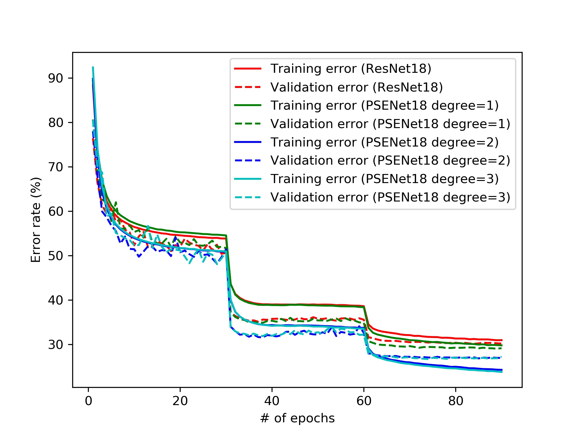
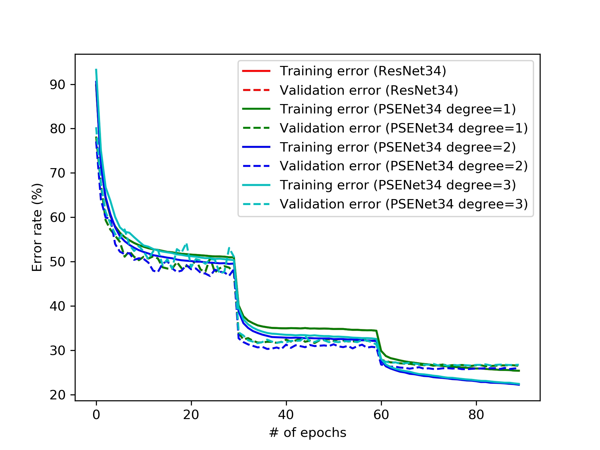
Figure 1: Error rates of image classification on ImageNet for ResNet and PSENet. Left: ResNet18 and PSENet18; right: ResNet34 and PSENet34. Notice: On the right panel, red lines (ResNet34) are overlapped by green lines (PSENet34 degree=1) and all experimental results shown above come from single optimization runs.

5 Conclusion

We develop a novel neural network by combing the ideas of PSE and the neural network approximation. Theoretically, we prove the better approximation result of PSENet by comparing with ReLU^k-DNN and the optimal approximation rate on singular functions. Moreover, the PSENet can achieve a better approximation accuracy on the shallow network structure in comparison with other neural networks. Several numerical results have been used to demonstrate the advantages of the PSENet. This new approach shows that increasing the degree of PSENet can also lead to further performance improvements rather than going deep. However, the performance can also decrease when the degree is larger than the optimal degree of PSENet. Obtaining an optimal degree by analysis is one of the future directions. Another interesting avenue to pursue is PSENet with other activation functions rather than ReLU. In this paper, our analysis and numerical results are based on ReLU activation function (or ReLU^k). But the novel PSENet architecture can define any activation function. Some challenges, such as weight initialization including $\alpha$ and approximation properties, will also be explored in the future.

References

- [1] Robert A Adams and John JF Fournier. Sobolev spaces. Elsevier, 2003.
- [2] R. Arora, A. Basu, P. Mianjy, and A. Mukherjee. Understanding deep neural networks with rectified linear units. In International Conference on Learning Representations, 2018.
- [3] S. Arora, N Cohen, and E. Hazan. On the optimization of deep networks: Implicit acceleration by overparameterization. In 35th International Conference on Machine Learning, 2018.
- [4] Ivo Babuška and Manil Suri. The p and h-p versions of the finite element method, basic principles and properties. SIAM review, 36(4):578–632, 1994.
- [5] A. Barron. Universal approximation bounds for superpositions of a sigmoidal function. IEEE Transactions on Information theory, 39(3):930–945, 1993.
- [6] Q. Chen and W. Hao. A homotopy training algorithm for fully connected neural networks. Proceedings of the Royal Society A, 475(2231):20190662, 2019.
- [7] A. Chernov, T. von Petersdorff, and C. Schwab. Exponential convergence of quadrature for integral operators with gevrey kernels. ESAIM: Mathematical Modelling and Numerical Analysis-Modélisation Mathématique et Analyse Numérique, 45(3):387–422, 2011.
- [8] C. de Boor. Subroutine package for calculating with b-splines. Los Alamos Scient. Lab. Report LA-4728-MS, 1971.
- [9] W. E and Q. Wang. Exponential convergence of the deep neural network approximation for analytic functions. Science China Mathematics, 61(10):1733–1740, 2018.
- [10] I. Gühring, G. Kutyniok, and P. Petersen. Error bounds for approximations with deep relu neural networks in norms. Analysis and Applications, 18(05):803–859, 2020.
- [11] W. Gui and I. Babuška. Theh, p andh-p versions of the finite element method in 1 dimension. Numerische Mathematik, 49(6):613–657, 1986.
- [12] J. He, L. Li, and J. Xu. Approximation properties of relu deep neural networks for smooth and non-smooth functions. In preparation, 2021.
- [13] J. He, L. Li, and J. Xu. Dnn with heaviside, relu and requ activation functions. In preparation, 2021.
- [14] J. He, L. Li, and J. Xu. Relu deep neural networks from the hierarchical basis perspective. arXiv preprint arXiv:2105.04156, 2021.
- [15] J. He, L. Li, J. Xu, and C. Zheng. Relu deep neural networks and linear finite elements. Journal of Computational Mathematics, 38(3):502–527, 2020.
- [16] K. He, X. Zhang, S. Ren, and J. Sun. Deep residual learning for image recognition. In Proceedings of the IEEE conference on computer vision and pattern recognition, pages 770–778, 2016.
- [17] L. Jones et al. A simple lemma on greedy approximation in hilbert space and convergence rates for projection pursuit regression and neural network training. The annals of Statistics, 20(1):608–613, 1992.
- [18] . Kang, S, W. Liao, and Y. Liu. Ident: Identifying differential equations with numerical time evolution. Journal of Scientific Computing, 87(1):1–27, 2021.
- [19] H. Lei, L. Wu, and E W. Machine-learning-based non-newtonian fluid model with molecular fidelity. Physical Review E, 102(4):043309, 2020.
- [20] J. Lu, Z. Shen, H. Yang, and S. Zhang. Deep network approximation for smooth functions. arXiv preprint arXiv:2001.03040, 2020.
- [21] L. Lu, X. Meng, Z. Mao, and G. Karniadakis. Deepxde: A deep learning library for solving differential equations. SIAM Review, 63(1):208–228, 2021.
- [22] Z. Lu, H. Pu, F. Wang, Z. Hu, and L. Wang. The expressive power of neural networks: A view from the width. In Advances in Neural Information Processing Systems, pages 6231–6239, 2017.
- [23] H. Montanelli, H. Yang, and Q. Du. Deep relu networks overcome the curse of dimensionality for bandlimited functions. arXiv preprint arXiv:1903.00735, 2019.
- [24] G. Montufar, R. Pascanu, K. Cho, and Y. Bengio. On the number of linear regions of deep neural networks. In Advances in neural information processing systems, pages 2924–2932, 2014.
- [25] J. Opschoor, P. Petersen, and C. Schwab. Deep relu networks and high-order finite element methods. Analysis and Applications, pages 1–56, 2020.
- [26] J. Opschoor, C. Schwab, and J. Zech. Exponential relu dnn expression of holomorphic maps in high dimension. SAM Research Report, 2019, 2019.
- [27] T. Poggio, H. Mhaskar, L. Rosasco, B. Miranda, and Q. Liao. Why and when can deep-but not shallow-networks avoid the curse of dimensionality: a review. International Journal of Automation and Computing, 14(5):503–519, 2017.
- [28] C. Schwab. p- and hp- Finite Element Methods: Theory and Applications to Solid and Fluid Mechanics. The Clarendon Press, Oxford University Press New York, 1998.
- [29] Jie Shen, Tao Tang, and Li-Lian Wang. Spectral methods: algorithms, analysis and applications, volume 41. Springer Science & Business Media, 2011.
- [30] Z. Shen, H. Yang, and S. Zhang. Deep network approximation characterized by number of neurons. arXiv preprint arXiv:1906.05497, 2019.
- [31] Z. Shen, H. Yang, and S. Zhang. Nonlinear approximation via compositions. Neural Networks, 119:74–84, 2019.
- [32] J. Siegel and J. Xu. High-order approximation rates for neural networks with reluk activation functions. arXiv preprint arXiv:2012.07205, 2020.
- [33] S. Tang, B. Li, and H. Yu. Chebnet: Efficient and stable constructions of deep neural networks with rectified power units using chebyshev approximations. arXiv preprint arXiv:1911.05467, 2019.
- [34] M. Telgarsky. Benefits of depth in neural networks. Journal of Machine Learning Research, 49(June):1517–1539, 2016.
- [35] B. Wang, D. Zou, Q. Gu, and S. Osher. Laplacian smoothing stochastic gradient markov chain monte carlo. SIAM Journal on Scientific Computing, 43(1):A26–A53, 2021.
- [36] J. Xu. The finite neuron method and convergence analysis. arXiv preprint arXiv:2010.01458, 2020.
- [37] I. Yaacov. A multivariate version of the vandermonde determinant identity. arXiv preprint arXiv:1405.0993, 8, 2014.
- [38] W. Zhu, Q. Qiu, B. Wang, J. Lu, G. Sapiro, and I. Daubechies. Stop memorizing: A data-dependent regularization framework for intrinsic pattern learning. SIAM Journal on Mathematics of Data Science, 1(3):476–496, 2019.