Semidefinite Relaxations of Products of Nonnegative Forms on the Sphere

Abstract.

We study the problem of maximizing the geometric mean of $d$ low-degree non-negative forms on the real or complex sphere in $n$ variables. We show that this highly non-convex problem is NP-hard even when the forms are quadratic and is equivalent to optimizing a homogeneous polynomial of degree $O(d)$ on the sphere. The standard Sum-of-Squares based convex relaxation for this polynomial optimization problem requires solving a semidefinite program (SDP) of size $n^{O(d)}$, with multiplicative approximation guarantees of $\Omega(\frac{1}{n})$. We exploit the compact representation of this polynomial to introduce a SDP relaxation of size polynomial in $n$ and $d$, and prove that it achieves a constant factor multiplicative approximation when maximizing the geometric mean of non-negative quadratic forms. We also show that this analysis is asymptotically tight, with a sequence of instances where the gap between the relaxation and true optimum approaches this constant factor as $d\rightarrow\infty$. Next we propose a series of intermediate relaxations of increasing complexity that interpolate to the full Sum-of-Squares relaxation, as well as a rounding algorithm that finds an approximate solution from the solution of any intermediate relaxation. Finally we show that this approach can be generalized for relaxations of products of non-negative forms of any degree.

1. Introduction

Sum-of-squares optimization is a powerful method of constructing hierarchies of relaxations for polynomial optimization problems that converge to the optimal solution at a cost of increasing computational complexity ([Las01], [Par00]). However, computing these relaxations in general requires solving large instances of semidefinite programs (SDPs), which quickly becomes computationally intractable. In particular, to find the Sum-of-Squares decomposition of a dense degree-$d$ polynomial in $n$ variables, the input size alone is of order $n^{O(d)}$, which is exponential in the degree.

In this paper, we introduce a series of Sum-of-Squares based algorithms to efficiently approximate a class of dense polynomial optimization problems where the polynomials have high degree (where the degree is comparable to the number of variables) but are compactly represented (meaning that they can be efficiently evaluated). One example of such a polynomial is the determinant of a $n\times n$ matrix, a degree $n$ polynomial in its $n^{2}$ entries (thus having exponentially many coefficients), but can be efficiently computed in polynomial time. The class of polynomials we study in this paper is constructed by taking the product of low-degree non-negative polynomials. For the most of the paper, we will focus on the product of positive semidefinite (PSD) forms, corresponding to the product of degree-2 non-negative polynomials.

Definition 1.1.

Let $\mathcal{A}=(A_{1},\ldots,A_{d})$ where $A_{i}\in\mathbb{K}^{n\times n}$ be symmetric/Hermitian PSD matrices, where $\mathbb{K}=\mathbb{R}\text{ or }\mathbb{C}$. Then

$$p(x)=\prod_{i=1}^{d}\left\langle x,A_{i}x\right\rangle,$$

a degree-$2d$ polynomial of $n$ variables, is a product of PSD forms.

Maximizing the product of PSD forms over the sphere generalizes many different problems in optimization, such as Kantorovich’s inequality, optimizing monomials over the sphere, linear polarization constants for Hilbert spaces, approximating permanents of PSD matrices, portfolio optimization, and can also be interpreted as computing the Nash social welfare for agents with polynomial utility functions. It also has connections to bounding the relative entropy distance between a quadratic map and its convex hull. These applications will be further elaborated in Section 2. We also prove in Section 7 that this problem is NP-hard when $d=\Omega(n)$, using a reduction to hardness of approximation of MaxCut. Since $d$ can be much greater than $n$, in order to normalize for $d$ we define our objective to be the geometric mean of quadratic forms:

(1) $$\textsc{Opt}(\mathcal{A})\coloneqq\max_{x\in\mathbb{K},\,\left\lVert x\right\lVert=1}\,\left(\prod_{i=1}^{d}\left\langle x,A_{i}x\right\rangle\right)^{1/d}.$$

Sum-of-Squares optimization allow us to create a hierarchy of algorithms of increasing complexity that give better bounds for (1). In general, if the objective is a degree $2d$ polynomial, the lowest level of the hierarchy is a degree-$d$ Sum-of-Squares relaxation. This relaxation for (1) is written as follows:

(2) $$\textsc{OptSOS}_{d}(\mathcal{A})\coloneqq\min\,\gamma^{1/d}\quad\text{s.t.}\quad\gamma\left\lVert x\right\lVert^{2d}-\prod_{i=1}^{d}\left\langle x,A_{i}x\right\rangle\text{ is a sum of squares},$$

where a polynomial $f(x)$ is a sum of squares if there exist polynomials $s_{i}(x)$ so that $f(x)=\sum_{i}s_{i}(x)^{2}$. The constraint that a degree $d$ polynomial in $n$ variables is a sum of squares can be represented by a SDP of size $n^{O(d)}$. Although techniques exist for reducing the size of this representation for sparse polynomials [KKW05] and polynomials with symmetry [GP04], the polynomial $p(x)$ may not have these properties. Thus $\textsc{OptSOS}_{d}(\mathcal{A})$ requires solving a SDP of size $n^{O(d)}$. However, because of the compact representation of this polynomial, one can perhaps hope to do better. In this paper we first present a SDP-based relaxation of $\textsc{Opt}(\mathcal{A})$ as well as a rounding algorithm for this relaxation.

Definition 1.2 (Semidefinite relaxation of (1)).

We define $\textsc{OptSDP}(\mathcal{A})$ to be the optimum of the following SDP-based relaxation of (1):

(5) $$\textsc{OptSDP}(\mathcal{A})\coloneqq\max_{X}\left(\prod_{i=1}^{d}\left\langle A_{i},X\right\rangle\right)^{1/d}\,\mbox{ s.t. }\,\left\{\begin{array}[]{rl}X&\succeq 0\\ \operatorname{Tr}(X)&=1\end{array}\right.,$$

where $X$ is symmetric when $\mathbb{K}=\mathbb{R}$ and Hermitian when $\mathbb{K}=\mathbb{C}$.

This relaxation comes from writing $\left\langle x,A_{i}x\right\rangle=\left\langle A_{i},xx^{\dagger}\right\rangle$ in (1) and relaxing the rank-1 matrix $xx^{\dagger}$ to the semidefinite variable $X$. Finding the value of this relaxation involves solving a SDP with $O(n^{2}+d)$ variables and $O(n^{2}d)$ constraints, compared to the Sum-of-Squares relaxation (2) which involves solving a SDP of size $n^{O(d)}$. The trade-off is that this relaxation is weaker than Sum-of-Squares (Proposition 6.6):

$$\textsc{Opt}(\mathcal{A})\leq\textsc{OptSOS}_{d}(\mathcal{A})\leq\textsc{OptSDP}(\mathcal{A}).$$

Nevertheless, we show that its approximation factor is bounded by a constant, compared to the worst case $\frac{1}{n}$ approximation factor of general polynomial optimization algorithms ([BGG⁺17], [DW12]). This comes from analyzing the following rounding algorithm which produces a feasible solution to (1) given an optimum solution $X^{*}$ to (5): Sample $y\sim\mathcal{N}_{\mathbb{K}}(0,X^{*})$ and return $x=y/\left\lVert y\right\lVert$, where $\mathcal{N}_{\mathbb{K}}$ is a real/complex multivariate Gaussian distribution (see Definition 4.1). The following theorem bounds the multiplicative approximation factor of the relaxation $\textsc{OptSDP}(\mathcal{A})$.

Theorem 1.3.

Suppose there is an optimal solution $X^{*}$ to (5) with $\operatorname{rank}(X^{*})=r$. Let

$$L_{r}(\mathbb{K}) =\ \begin{cases}\gamma+\log 2+\psi\left(\frac{r}{2}\right)-\log\left(\frac{r}{2}\right)<1.271&\text{ if }\mathbb{K}=\mathbb{R}\\ \gamma+\psi(r)-\log(r)<0.578&\text{ if }\mathbb{K}=\mathbb{C}\end{cases},$$

where $\psi(x)=\frac{d}{dx}\log\Gamma(x)$ is the digamma function. Then

$$e^{-L_{r}(\mathbb{K})}\textsc{OptSDP}(\mathcal{A})\leq\textsc{Opt}(\mathcal{A})\leq\textsc{OptSDP}(\mathcal{A}),$$

which gives us a multiplicative approximation factor of $e^{-L_{r}(\mathbb{K})}$.

Since $\lim_{r\rightarrow\infty}\psi(r)-\log(r)=0$, the approximation factor is at least $0.2807$ when $\mathbb{K}=\mathbb{R}$ and $0.5614$ when $\mathbb{K}=\mathbb{C}$, and can be improved if we can further bound $\operatorname{rank}(X^{*})$. In particular, since $L_{1}(\mathbb{K})=0$, the rounding algorithm recovers the exact solution when $\operatorname{rank}(X^{*})=1$. In section 3 we explore a few cases where this relaxation is exact, showing that the relaxation (5) is able to exactly recover Kantorovich’s inequality (Example 3.2), as well as find the exact optimal solution for optimizing any monomial over the sphere (Section 3.3).

Using a connection to linear polarization constants (Section 5), we show that there exists an asymptotically tight integrality gap instance where the gap between $\textsc{Opt}(\mathcal{A})$ and $\textsc{OptSDP}(\mathcal{A})$ approaches the approximation factor $e^{-L_{r}(\mathbb{K})}$ as $n$ and $d$ approaches infinity. The intuition is to choose $A_{i}=v_{i}v_{i}^{\dagger}$ to be rank-1, where $v_{i}$ are symmetrically distributed on the sphere. Because of symmetry, the rounding algorithm on this instance will sample a uniformly random point on the sphere, completely ignoring the structure of the problem. We plot an example of such a symmetric polynomial in Figure 1.

This also motivates the need for higher-degree relaxations that perform better than (5). In Section 6, we define a series of Sum-of-Squares based relaxations computing $\textsc{OptSOS}_{k}(\mathcal{A})$, which interpolates between $\textsc{OptSOS}_{1}(\mathcal{A})=\textsc{OptSDP}(\mathcal{A})$ and $\textsc{OptSOS}_{d}(\mathcal{A})$, the full Sum-of-Squares relaxation. We also propose a randomized rounding algorithm which allows us to sample a feasible solution from the relaxation. Figure 1 shows the distribution sampled from this rounding algorithm for different values of $k$ for a “worst case” example with multiple global optima symmetrically distributed on the sphere. We can see that the sampled distribution concentrates towards the true optimum values as $k$ increases. We then analyze the approximation ratio of the rounding algorithm and provide lower bounds on the integrality gap similar to the results in Section 5. Next we extend this relaxation to products of general non-negative forms. Finally in Section 7, we prove a hardness of approximation result for computing $\textsc{Opt}(\mathcal{A})$ by a reduction to MaxCut.

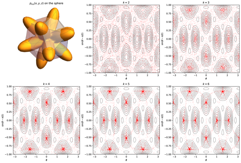
Figure 1. $p_{\text{ico}}(x,y,z)$ is a degree 6 polynomial in 3 variables with icosahedral symmetry (see Example 6.4 for its definition). The 3D plot shows the value of $p_{\text{ico}}$ on the sphere, superimposed on an icosahedron. We compute $\textsc{OptSOS}_{k}$ for $k=2,\ldots,6$, relaxations of maximizing $p_{\text{ico}}(x,y,z)$ over the 2-sphere. The 2D plots show samples from the distribution obtained by the rounding algorithm to $\textsc{OptSOS}_{k}$, on an equal-area projection of the sphere. The contour plot is of $p_{\text{ico}}$ and shows its 12 maxima on the sphere, and is overlaid on a scatter plot of 10000 points sampled by the rounding algorithm.

1.1. Related Work

There has been recent attention on problems similar to (1). The authors of this paper analyzed a special case of (1) where the $A_{i}$ are rank-1 matrices, used in an approximation algorithm for the permanent of PSD matrices [YP21] (see Section 2.5 for more details). To the best of our knowledge, the first constant-factor approximation algorithm to (1) is given in [Bar14], and is used to prove that the quadratic map $x\mapsto(\left\langle x,A_{1}x\right\rangle,\ldots,\left\langle x,A_{d}x\right\rangle)$ is close to its convex hull in relative entropy distance. Our work improves on this constant, and our result in Section 5 show that it cannot be further improved. Barvinok [Bar93] also reduced the problem of certifying feasibility for systems of quadratic equations to finding the optimum of (1), and provided a polynomial time algorithm for solving (1) when $d$ is fixed. A more recent work [Bar20] studied a closely related problem of approximating the integral of a product of quadratic forms on the sphere, giving a quasi-polynomial time approximation algorithm.

For general polynomial optimization on the sphere, [DW12], [BGG⁺17] and [FF20] gave bounds on the convergence of the Sum-of-Squares hierarchy. These papers analyzed the convergence of higher levels of the hierarchy (of which $\textsc{OptSOS}_{d}(\mathcal{A})$ is the lowest level), proposed rounding algorithms and bounded their approximation ratios. As noted in the introduction, these methods when applied to (1) takes $n^{O(d)}$ time and only guarantees a $\Omega(1/n)$ approximation ratio, as $p(x)$ is a high degree polynomial.

Finally, we review some strategies for speeding up Sum-of-Squares for different polynomial optimization problems with special structure:

1. Solving the problem using a weakened but more computationally efficient version of sum of squares, for example using diagonally-dominant or scaled-diagonally-dominant cones instead of the positive semidefinite cone [AH17]. These methods typically sacrifice solution quality for computational tractability, but bounds on their approximation quality are not known.

2. Reducing the size of SDPs needed by exploiting special structure in the problem, such as sparsity in [KKW05] and [FSP16] or symmetry in [GP04].

3. Using spectral methods inspired by sum of squares algorithms to solve average case problems [HSSS15] [HKP⁺17]. They show that there exist spectral algorithms that are almost as good as sum of squares algorithms for a variety of planted problems.

From the above works we can see that there is a trade-off between how much structure the problem class has, how much faster the sped-up algorithm is and how much accuracy it loses compared to running the full Sum-of-Squares algorithm. Our work uses the compact representation of the product of non-negative forms to arrive at the relaxation (5). This is much faster and has much better approximation guarantees than the standard Sum-of-Squares relaxation of general polynomial optimization on the sphere.

1.2. Contributions

In summary, the main contributions of this paper are:

1. An SDP-based relaxation (5) and a simple randomized rounding procedure that finds a feasible solution to (1). We then prove that this is a constant-factor approximation algorithm to (1) (Theorem 1.3).

2. Using a connection to the linear polarization constant problem (Section 2.3) to show an integrality gap (Theorem 5.1) in the relaxation (5) that asymptotically matches the approximation factor shown in Theorem 1.3 as $d\rightarrow\infty$.

3. A strategy (Section 6) to turn degree-2 Sum-of-Squares relaxations of (1) into degree-$k$ relaxations for any $k\leq d$, as a way of interpolating between the relaxation (5) and the full degree-$d$ Sum-of-Squares relaxation. We also propose and implement a rounding algorithm to produce feasible solutions from these relaxations.

4. We also prove a hardness result from a reduction to MaxCut (Section 7), showing that in the regime $d=\Omega(n)$, the problem (1) is NP-hard.

1.3. Notations

In subsequent sections, we use $\mathbb{K}$ to denote either $\mathbb{R}$ or $\mathbb{C}$. For any $x\in\mathbb{C}$, let $x^{*}$ be its complex conjugate, and $\left|x\right|^{2}=xx^{*}$. For any matrix $A\in\mathbb{K}^{n\times m}$, let $A^{\dagger}=(A^{*})^{T}$ be its conjugate transpose if $\mathbb{K}=\mathbb{C}$, or its transpose if $\mathbb{K}=\mathbb{R}$. Given $a,b\in\mathbb{K}^{n}$, let $\left\langle a,b\right\rangle=a^{\dagger}b$ be its inner product in $\mathbb{K}^{n}$, and $\left\lVert a\right\lVert^{2}=\left\langle a,a\right\rangle$. A matrix $A$ is Hermitian if $A=A^{\dagger}$, and is positive semidefinite (PSD) if in addition $x^{\dagger}Ax\geq 0$ for all $x\in\mathbb{K}$. We can also denote this as $A\succeq 0$. The $\succeq$ operator induces a partial order called the Löwner order, where $A\succeq B$ if $A-B\succeq 0$.

2. Motivation and Applications

In this section we introduce a variety of problems that can be cast into (1), maximizing the geometric mean of PSD forms over the sphere. In particular, for a few special cases the relaxation OptSDP is exact, corresponding to when $d=2$ (Kantorovich’s inequality in Section 2.1) or $A_{i}$ are diagonal (optimizing monomials over sphere in Section 2.2 and portfolio optimization in Section 2.6). This shows that our approach generalizes many other optimization methods and has applications to problems such as finding the linear polarization constant of Hilbert spaces (Section 2.3), bounding the relative entropy distance between a quadratic map and its convex hull (Section 2.4), and approximating the permanent of PSD matrices (Section 2.5).

2.1. Kantorovich’s Inequality

Proposition 2.1 ([Kan48]).

Given a symmetric $n\times n$ positive definite matrix $A$, let $\lambda_{1}\geq\cdots\geq\lambda_{n}>0$ be its eigenvalues. Then for all $x\in\mathbb{R}^{n}$:

(6) $$\frac{(x^{\dagger}Ax)(x^{\dagger}A^{-1}x)}{x^{\dagger}x}\leq\frac{1}{4}\left(\sqrt{\frac{\lambda_{1}}{\lambda_{n}}}+\sqrt{\frac{\lambda_{n}}{\lambda_{1}}}\right)^{2}$$

This inequality is used in the analysis of the convergence rate for gradient descent (with exact line search) on quadratic objectives $x^{\dagger}Ax+b^{\dagger}x$ (see, for example, [LY08]). It is used to prove that the error decreases by a factor of $\left(\frac{\lambda_{1}-\lambda_{n}}{\lambda_{1}+\lambda_{n}}\right)^{2}$ with each step taken. It can also be used to bound the efficiency of estimators in noisy linear regression where $A$ is the covariance matrix of the noise [Rag86]. The optimization problem (1) is a generalization of this inequality to higher degree products. However unlike in (6) the $A_{i}$ may not be simultaneously diagonalizable.

2.2. Optimizing Monomials over the Sphere

Maximizing monomials on the sphere is a special case of (1) where $A_{i}$ are diagonal. We can compute the exact value of the maximum of any monomial over the sphere, and we have the following result for $\mathbb{K}=\mathbb{R}$ (a similar result holds for $\mathbb{K}=\mathbb{C}$).

Proposition 2.2.

Let $x^{\beta}=\prod_{i=1}^{n}x_{i}^{\beta_{i}}$ be any monomial of degree $d=\sum_{i}\beta_{i}$. Then

$$\max_{\left\lVert x\right\lVert=1,\,x\in\mathbb{R}^{n}}\left(x^{\beta}\right)^{\frac{2}{d}}=\frac{1}{d}\prod_{i=1}^{n}\beta_{i}^{\beta_{i}/d}$$

This result is proven in Appendix B. Since we know the exact value for this special case, it is useful to use this problem to compare different methods of speeding up Sum-of-Squares. In particular, the algorithms derived from Sum-of-Squares in ([HSSS15] and [BGG⁺17]) lose the structure of this problem and do not return the exact optimum. We will see in section 3.3 that our relaxation preserves this structure and is exact in this case.

2.3. Linear Polarization Constants for Hilbert Spaces

When all the $A_{i}$ in (1) are rank-1, the optimization problem has connections to the linear polarization constant problem:

Definition 2.3 (Linear polarization constant of a normed space).

Given a normed space $X$, let $X^{*}$ be its dual and $\mathcal{S}_{X}=\{x\in X:\left\lVert x\right\lVert=1\}$ be the sphere with respect to the norm. Then the $d$-th linear polarization constant of $X$ is given by:

$$c_{d}(X)\coloneqq\left(\inf_{f_{1},\ldots,f_{d}\in S_{X^{*}}}\sup_{x\in S_{X}}\left|f_{1}(x)\cdots f_{d}(x)\right|\right)^{-1}$$

This problem has been studied in the papers [PR04], [Mar97], and [MM06]. In particular, it is proved in [Ari98] that $c_{d}(\mathbb{C}^{d})=d^{d/2}$, but the analogous result for $\mathbb{R}^{d}$ is still a conjecture:

Conjecture 2.4 ([PR04]).

Let $v_{1},\ldots,v_{d}$ and $x$ be vectors in $\mathbb{R}^{d}$.

(7) $$\min_{\left\lVert v_{1}\right\lVert=1,\ldots,\left\lVert v_{d}\right\lVert=1}\max_{\left\lVert x\right\lVert=1}\left|\prod_{i=1}^{d}\left\langle v_{i},x\right\rangle\right|=d^{-d/2}$$

And is achieved when $v_{i}$ are (up to rotation) the basis vectors $e_{i}$.

We see that (7) is a minimax problem with its inner maximization problem equivalent to solving the following optimization problem:

(8) $$\max_{\left\lVert x\right\lVert=1}\left(\prod_{i=1}^{d}\left\langle v_{i},x\right\rangle^{2}\right)^{1/d}$$

Which is exactly (1) with $A_{i}=v_{i}v_{i}^{\dagger}$. Exact values for $c_{d}(\mathbb{K}^{n})$ where $\mathbb{K}=\mathbb{R}\text{ or }\mathbb{C}$ and $d>n$ are not known, but [PR04] computed the asymptotic value $\lim_{d\rightarrow\infty}c_{d}(\mathbb{K}^{n})^{1/d}$. We will use these results later to construct integrality gap instances in Sections 5 and 6.5.

2.4. Distance of a Quadratic Map to its Convex Hull

Given $A_{1},\ldots,A_{d}\succ 0$, let $\varphi(x):\mathbb{K}^{n}\rightarrow\mathbb{R}_{+}^{d}$ be a quadratic map that maps $x$ to $(\left\langle x,A_{1}x\right\rangle,\ldots,\left\langle x,A_{d}x\right\rangle)$. The convexity of the image of $\mathbb{K}^{n}$ by this map has many implications in controls and optimization (see, for example [PT07]). The set $\varphi(\mathbb{K}^{n})$ is not convex in general, although it is for special cases (such as when $d=2$). On the other hand, $\operatorname{conv}(\varphi(\mathbb{K}^{n}))$ has a semidefinite representation. Barvinok [Bar14] investigated how well $\operatorname{conv}(\varphi(\mathbb{K}^{n}))$ approximates $\varphi(\mathbb{K}^{n})$ in the relative entropy distance. Since both sets are cones in the non-negative orthant, it is natural to compare the size of their intersection with the simplex $\Delta_{d}=\{x\in\mathbb{R}^{d}\mid x_{i}\geq 0,\,\sum_{i}x_{i}=1\}$.

Theorem 2.5 (Theorem 1 in [Bar14]).

Let $a\in\operatorname{conv}(\varphi(\mathbb{R}^{n}))\cap\Delta_{d}$. Then there exists a point $b\in\varphi(\mathbb{R}^{n})\cap\Delta_{d}$ and an absolute constant $\beta=4.8>0$ such that

(9) $$\sum_{i=1}^{d}a_{i}\ln\left(\frac{a_{i}}{b_{i}}\right)\leq\beta.$$

Next we show how we can use proof of Theorem 1.3 to improve the constant $\beta$, as well as extend the result to $\mathbb{C}^{n}$. Since $a\in\operatorname{conv}(\varphi(\mathbb{K}^{n}))$, we can find $X\succeq 0$ such that $a_{i}=\left\langle A_{i},X\right\rangle$. If we let $L=\sum_{i}A_{i}\succ 0$, $A^{\prime}_{i}=L^{-1/2}A_{i}L^{-1/2}$ and $X^{\prime}=L^{1/2}XL^{1/2}$, we have $\operatorname{Tr}(X^{\prime})=\sum_{i}\left\langle A^{\prime}_{i},X^{\prime}\right\rangle=\sum_{i}a_{i}=1$. Now if we sample $z\sim\mathcal{N}_{\mathbb{K}}(0,X^{\prime})$ and let $y=z/\left\lVert z\right\lVert$, then from the proof of Theorem 4.6, we have

$$\mathop{{}\mathbb{E}}_{y}\left[\sum_{i}a_{i}\log\left\langle y,A^{\prime}_{i}y\right\rangle\right]\geq-L_{r}(\mathbb{K})+\sum_{i}a_{i}\log\left\langle A^{\prime}_{i},X^{\prime}\right\rangle,$$

where $r$ is the rank of $X^{\prime}$ satisfying $\left\langle A^{\prime}_{i},X^{\prime}\right\rangle=a_{i}$ and $\operatorname{Tr}(X^{\prime})=1$. If we let $b_{i}=\left\langle y,A^{\prime}_{i}y\right\rangle$, we can choose $\beta=L_{r}(\mathbb{K})$ in (9). Furthermore, Theorem 5.1 shows that this constant is asymptotically tight.

2.5. Permanents of PSD Matrices

Given a matrix $M\in\mathbb{C}^{n\times n}$, its permanent is defined to be

$$\operatorname{per}(M)=\sum_{\sigma\in\mathbf{S}_{n}}\prod_{i=1}^{n}M_{i,\sigma(i)},$$

Where the sum is over all permutations of $n$ elements. If $M$ is Hermitian positive semidefinite (PSD), [AGGS17] and [YP21] analyzed a SDP-based approximation algorithm that produces a simply exponential approximation factor to $\operatorname{per}(M)$. Let $M=V^{\dagger}V$ and $v_{i}$ are the columns of $V$. In [YP21], the problem of approximating $\operatorname{per}(M)$ is related to the problem of maximizing a product of linear forms over the complex sphere

$$r(M)\coloneqq\max_{\left\lVert x\right\lVert^{2}=n}\prod_{i=1}^{n}\left|\left\langle x,v_{i}\right\rangle\right|^{2},$$

and its convex relaxation $\operatorname{rel}(M)$ (obtained in a similar manner as (5)) by showing that

$$\frac{n!}{n^{n}}r(M)\leq\operatorname{per}(M)\leq\operatorname{rel}(M).$$

Thus we can approximate $\operatorname{per}(M)$ by analyzing the approximation quality of $\operatorname{rel}(M)$ as a relaxation of $r(M)$. It is easy to see that $r(M)$ is equivalent to a special case of (1) when the $A_{i}$ are all rank-1, and the result of Theorem 1.3 applied to this problem gives the same approximation factor to the permanent as [YP21].

2.6. Portfolio Optimization

Suppose there is a collection of $n$ stocks with their returns denoted as $r$, where $r_{i}>0$ denotes the return of stock $i$ ($r_{i}<1$ making a loss and $r_{i}>1$ making a profit). We wish to select a mix of these stocks to invest in, allotting a fraction $y_{i}$ of our capital to stock $i$ so as to maximize our expected return. We have the historical returns $r(1),\ldots,r(d)$ over $d$ time periods to base our decision on. The strategy employed by [WPM77] is to maximize the geometric mean of the total returns

$$\max_{y\geq 0,\sum_{i}y_{i}=1}\left(\prod_{i=1}^{d}\left\langle y,r(i)\right\rangle\right)^{1/d},$$

which can be interpreted as rebalancing the portfolio after each time period. This is a special case of (1) in which $A_{i}$ are diagonal matrices with $r(i)$ on the diagonal and $y_{i}=x_{i}^{2}$. In Section 3.5 we show that in this case the relaxation (5) is exact.

2.7. Nash Social Welfare

Suppose $x$ is an allocation of a set of divisible resources to $d$ agents each with a non-negative utility function $A_{i}(x)$. We can ensure fairness by choosing the objective function, which result in different notions of fairness, ranging from the utilitarian $\max_{x}\frac{1}{d}\sum_{i}A_{i}(x)$ to egalitarian $\max_{x}\min_{i}A_{i}(x)$. Interpolating between these is the Nash social welfare objective $\max_{x}\left(\prod_{i}A_{i}(x)\right)^{1/d}$, which is the geometric mean of the utilities. This objective is well-studied for allocation of indivisible items [CKM⁺16], from hardness results [Lee17] to constant factor approximation algorithms [AGSS17]. In our setting, the utility function for agent $i$ is $x^{\dagger}A_{i}x$, a non-negative quadratic form on $x$.

3. Semidefinite Relaxation

Before proving Theorem 1.3, we derive our semidefinite relaxation of the problem and give interpretations for both its primal and dual forms. The insights gained from deriving both the primal and dual relaxations will be helpful in Section 6 when generalizing to higher-degree relaxations. Recall that the polynomial we wish to optimize is

$$p_{\mathcal{A}}(x)=\prod_{i=1}^{d}\left\langle x,A_{i}x\right\rangle,$$

and we want to find an upper bound of $p_{\mathcal{A}}(x)^{1/d}$ on the sphere. One can compute an upper bound using the degree-$d$ Sum-of-Squares relaxation (2) over the sphere, but this involves solving a SDP of size $n^{O(d)}$, which is computationally inefficient and does not exploit the compact representation of $p_{\mathcal{A}}(x)$. One computationally efficient upper bound is given by $\prod_{i=1}^{d}\left\lVert A_{i}\right\lVert^{1/d}$, the geometric mean of the spectral norms of $A_{i}$, but it can differ from the true optimum multiplicatively by a factor of $n^{-1/2}$ (see Proposition 2.2). In the next few sections, we will introduce a series of weaker but computationally more efficient bounds, which still have good approximation guarantees.

3.1. Quadratic Upper Bounds

The first approach uses the arithmetic mean/geometric mean (AM/GM) inequality:

$$\left(\prod_{i=1}^{d}\left\langle x,A_{i}x\right\rangle\right)^{\frac{1}{d}}\leq\frac{1}{d}\sum_{i=1}^{d}\left\langle x,A_{i}x\right\rangle=\frac{1}{d}\,x^{\dagger}\left(\sum_{i=1}^{d}A_{i}\right)x$$

This then becomes an eigenvalue problem. Maximizing this quadratic form over the unit sphere, we obtain the following:

Proposition 3.1.

Let $G=\sum_{i=1}^{d}A_{i}$. Then if $\left\lVert x\right\lVert=1$,

$$p_{\mathcal{A}}(x)\leq\left(\frac{\lambda_{\max}(G)}{d}\right)^{d}.$$

This technique is powerful enough to prove Kantorovich’s inequality (Proposition 2.1), as we will see in the following example. This is a adaptation of Newman’s proof in [New60].

Example 3.2 (Proof of Kantorovich’s inequality).

Since both $A$ and $A^{-1}$ are positive definite, we can apply the AM/GM inequality on $(\alpha x^{\dagger}Ax)(\alpha^{-1}x^{\dagger}A^{-1}x)$ for any $\alpha>0$:

$$(x^{\dagger}Ax)(x^{\dagger}A^{-1}x)\leq\frac{1}{4}\left(x^{\dagger}\left(\frac{1}{\alpha}A+\alpha A^{-1}\right)x\right)^{2}\leq\frac{1}{4}\lambda_{\max}\left(\frac{1}{\alpha}A+\alpha A^{-1}\right)^{2}.$$

Without loss of generality we assume $A$ and $A^{-1}$ are diagonal, as they are simultaneously diagonalizable. Choosing $\alpha=\sqrt{\lambda_{1}\lambda_{n}}$,

$$\lambda_{\max}\left(\frac{1}{\alpha}A+\alpha A^{-1}\right)=\max_{i}\left(\frac{\lambda_{i}}{\sqrt{\lambda_{1}\lambda_{n}}}+\frac{\sqrt{\lambda_{1}\lambda_{n}}}{\lambda_{i}}\right)\leq\sqrt{\frac{\lambda_{1}}{\lambda_{n}}}+\sqrt{\frac{\lambda_{n}}{\lambda_{1}}}.$$

This is because $f(x)=\frac{x}{\alpha}+\frac{\alpha}{x}$ is convex on any nonnegative interval and a convex function on an interval is maximized at its endpoints.

3.2. Rescaling and Semidefinite Relaxation

In Example 3.2, in addition to using the AM/GM inequality, we also introduced a scaling factor $\alpha$ to strengthen the inequality. Since the cost function is multilinear in $A_{i}$, we can optimize over all possible rescalings $A_{i}\mapsto\alpha_{i}A_{i}$ for all $\alpha_{i}>0$ where $\prod_{i}\alpha_{i}=1$, to improve the upper bound. Furthermore, the problem of optimizing over such scalings is also convex since a lower bound on the concave geometric mean $\left(\prod_{i=1}^{d}\alpha_{i}\right)^{1/d}$ defines a convex set.

Theorem 3.3.

Given $\mathcal{A}=(A_{1},\ldots,A_{d})$, the following upper bound holds:

$$\textsc{Opt}(\mathcal{A})=\max_{\left\lVert x\right\lVert=1}p_{\mathcal{A}}(x)^{1/d}\leq\lambda^{*},$$

where $\lambda^{*}$ is the optimum of the following convex program:

(10) $$\min\lambda\quad\text{s.t.}\quad\frac{1}{d}\sum_{i=1}^{d}\alpha_{i}A_{i}\preceq\lambda I_{n},\quad\prod_{i=1}^{d}\alpha_{i}\geq 1,\quad\alpha_{i}>0$$

Next by taking the dual, we relate the optimum value of (10) with that of (5), which also proves the upper bound in Theorem 1.3.

Theorem 3.4.

The following upper bound holds:

$$\textsc{Opt}(\mathcal{A})\leq\textsc{OptSDP}(\mathcal{A}),$$

where $\textsc{OptSDP}(\mathcal{A})$ is the optimum of the following convex program:

(13) $$\textsc{OptSDP}(\mathcal{A})\coloneqq\max\left(\prod_{i=1}^{d}\left\langle A_{i},X\right\rangle\right)^{1/d}\quad\mbox{ s.t. }\quad\left\{\begin{array}[]{rl}\operatorname{Tr}(X)&=1\\ X&\succeq 0\end{array}\right.$$

Furthermore, (13) is dual to (10), and $\textsc{OptSDP}(\mathcal{A})=\lambda^{*}$.

Proof.

It is clear that $\textsc{OptSDP}(\mathcal{A})$ is a rank relaxation of $\textsc{Opt}(\mathcal{A})$, by using the variable $X$ instead of $xx^{\dagger}$. To find the dual of (10), we write the Lagrangian

$$\mathcal{L}(X,\gamma,\alpha,\lambda)=\lambda-\left\langle\lambda I-\frac{1}{d}\sum_{i=1}^{d}\alpha_{i}A_{i},X\right\rangle-\gamma\left(\prod_{i}\alpha_{i}^{1/d}-1\right)$$

Solving for $\lambda$, we get the constraint $\operatorname{Tr}(X)=1$. Solving for $\alpha_{i}$ and $\gamma$, we get

$$\alpha_{i}=\frac{\gamma}{\left\langle A_{i},X\right\rangle}\text{ and }\gamma=\left(\prod_{i=1}^{d}\left\langle A_{i},X\right\rangle\right)^{1/d}$$

And we obtain (13) after substituting these values into the Lagrangian. ∎

Note that the dual objective is log-concave, and it is a special case of maximizing the determinant of a PSD matrix, which can be solved efficiently using (for example) interior point methods [VBW98].

3.3. Maximizing Monomials over the Sphere

To get more insight of the role the multipliers $\alpha_{i}$ play, we consider the special case where $p(x)=x^{2\beta}$ is a monomial. Maximizing a monomial over the sphere is a special case of (1): for each copy of $x_{i}$ in $x^{\beta}$ (there are $d$ of these in total, corresponding to $A_{1},\ldots,A_{d}$), set $A_{j}$ to be 1 on the $i$-th diagonal entry and 0 elsewhere. Next we show that the convex relaxation in Theorem 3.3 achieves the true maximum value. In the relaxation there are $d$ multipliers $\alpha_{1},\ldots,\alpha_{d}$ associated with each copy of $x_{i}$. For each $x_{i}$, set its multiplier to be $\beta_{i}^{-1}\prod_{i=1}^{n}{\beta_{i}}^{\beta_{i}/d}$. Thus

$$\lambda_{\max}\left(\frac{1}{d}\sum_{j=1}^{d}\alpha_{j}A_{j}\right)=\lambda_{\max}\left(\frac{1}{d}\sum_{j=1}^{n}\sum_{k=1}^{\beta_{j}}\beta_{j}^{-1}\prod_{i=1}^{n}{\beta_{j}}^{\beta_{j}/d}e_{j}e_{j}^{\dagger}\right)=\frac{1}{d}\prod_{i=1}^{n}{\beta_{j}}^{\beta_{j}/d}$$

Thus the relaxation value is the same as the optimum given by Proposition 2.2. The multipliers $\alpha_{i}$ play the role of balancing out the terms in the sum.

3.4. Rank of Solutions

We can bound the rank of the solution $X^{*}$ to the relaxation (13) using a result by Barvinok [Bar02] and Pataki [Pat98]:

Proposition 3.5 (Proposition 13.4 of [Bar02]).

For some $r>0$, fix $k=(r+2)(r+1)/2$ symmetric matrices $A_{1},\ldots,A_{k}\in\mathbb{R}^{n\times n}$ where $n\geq r+2$ and $k$ real numbers $\alpha_{1},\ldots,\alpha_{k}$. If there is a solution $X\succeq 0$ to the system:

$$\left\langle A_{i},X\right\rangle=\alpha_{i}\quad\text{ for }\quad i=1,\ldots,k$$

and the set of all such solutions is bounded, then there is a matrix $X_{0}\succeq 0$ satisfying the same system and $\operatorname{rank}X_{0}\leq r$.

Indeed, suppose $X^{*}$ is an optimal solution to the relaxation (5), then any solution $X$ to the $d+1$ linear equations $\left\langle X,A_{i}\right\rangle=\left\langle X^{*},A_{i}\right\rangle$ and $\operatorname{Tr}(X)=1$ is also optimal. Proposition 3.5, along with an analogous result in the complex setting [AHZ08], also implies that the rank of the relaxation is bounded by $O(\sqrt{d})$, which helps us bound the approximation factor of this relaxation in the next section.

3.5. Exact Relaxations

In this section we study a few special cases where the relaxation $\textsc{OptSDP}(\mathcal{A})$ is exact. The first case is when $d=2$, which is a direct result of Proposition 3.5 substituting in $k=3$.

Proposition 3.6.

When $d=2$ and $\mathbb{K}=\mathbb{R}$, then $\textsc{Opt}(\mathcal{A})=\textsc{OptSDP}(\mathcal{A})$.

This also implies that the bound on Kantorovich’s inequality produced by our relaxation is tight. Next we show that the relaxation is tight when $A_{i}$ are simultaneously diagonalizable. This also implies that our relaxation finds the optimum solutions to the portfolio optimization (Section 2.6) and optimizing monomial (Section 2.2) problems.

Proposition 3.7.

Let $\mathcal{A}=(A_{1},\ldots,A_{d})$. If all $A_{i}$ commute with each other, then $\textsc{Opt}(\mathcal{A})=\textsc{OptSDP}(\mathcal{A})$.

Proof.

Since the matrices $A_{i}$ commute with each other, they are simultaneously diagonalizable. They can be written as $A_{i}=U^{\dagger}D_{i}U$, where $D_{i}$ is diagonal and $U$ unitary. Then after a change of variables $x\mapsto Ux$, the relaxation (5) is equivalent to the original problem (1) with the substitution $X_{ii}=x_{i}^{2}$. ∎

4. Rounding Algorithm and Analysis

In this section we present our randomized rounding algorithm for the relaxation $\textsc{OptSDP}(\mathcal{A})$ (5), and an analysis of its approximation factor (Theorem 1.3). First we state some standard results about generalized Chi-squared distributions, after which we will use these results to prove Theorem 1.3.

4.1. Background on Real and Complex Multivariate Gaussians

In this section we will use a few results involving the expectation of functions of real or complex multivariate Gaussian variables.

Definition 4.1 (Multivariate Gaussian Random Variable).

Let $x\sim\mathcal{N}_{\mathbb{K}}(0,I_{n})$. If $\mathbb{K}=\mathbb{R}$, then its coordinates $x_{j}$ are i.i.d. normal random variables. If $\mathbb{K}=\mathbb{C}$, then $x_{j}=(y_{j}+iz_{j})/\sqrt{2}$, where $y_{j}$ and $z_{j}$ are i.i.d. standard normal random variables.

The random variable $z\sim\mathcal{N}_{\mathbb{C}}(0,I_{n})$ is circularly symmetric, meaning that its distribution is invariant after the transformation $z\mapsto e^{i\theta}z$ for all $\theta\in\mathbb{R}$. All complex multivariate Gaussians in this paper are circularly symmetric. Similar to real multivariate Gaussians, a linear transform on the random vector induces a congruence transform on the covariance matrix.

Proposition 4.2 (Invariance under orthogonal/unitary transformations).

Given $x\sim\mathcal{N}_{\mathbb{K}}(0,\Sigma)$ and any matrix $A\in\mathbb{K}^{n\times n}$, $Ax$ has the distribution $\mathcal{N}_{\mathbb{K}}(0,A\Sigma A^{\dagger})$.

Thus given $A=UU^{\dagger}\succeq 0$, to sample $w\in\mathbb{K}^{n}$ from $\mathcal{N}_{\mathbb{K}}(0,A)$, we can first sample $x\sim\mathcal{N}_{\mathbb{K}}(0,I)$, then let $w=Ux$. The proof of this proposition and more about complex multivariate Gaussians can be found in [Gal]. In particular, this tells us that the distribution $\mathcal{N}_{\mathbb{K}}(0,I)$ is invariant under unitary transformations.

In the analysis of our rounding procedure, we use some results about the gamma distribution.

Fact 4.3 (Expectation of log of gamma random variable).

Let $X\sim\operatorname{Gamma}(\alpha,\beta)$ be drawn from the gamma distribution, with density $p(x;\alpha,\beta)=\Gamma(\alpha)^{-1}\beta^{\alpha}x^{\alpha-1}e^{-\beta x}$. Then

$$\mathop{{}\mathbb{E}}[\log X]=\psi(\alpha)-\log(\beta),$$

where $\psi(x)=\frac{d}{dx}\log\Gamma(x)$ is the digamma function.

This follows from the fact that the gamma distribution is an exponential family, of which $\log x$ is a sufficient statistic (see section 2.2 of [Kee10] for more details). Next we prove an useful identity.

Fact 4.4.

Let $(z_{1},\ldots,z_{r})\sim\mathcal{N}_{\mathbb{K}}(0,I_{r})$, $\gamma=\lim_{n\rightarrow\infty}(H_{n}-\log n)\approx 0.577$ be the Euler-Mascheroni constant and

$$L_{r}(\mathbb{K}) =\ \begin{cases}\gamma+\log 2+\psi\left(\frac{r}{2}\right)-\log\left(\frac{r}{2}\right)&\text{ if }\mathbb{K}=\mathbb{R}\\ \gamma+\psi(r)-\log(r)&\text{ if }\mathbb{K}=\mathbb{C}\end{cases}.$$

Then

$$\mathop{{}\mathbb{E}}\left[\log\left(\frac{1}{r}\sum_{i=1}^{r}\left|z_{i}\right|^{2}\right)\right]=\mathop{{}\mathbb{E}}\left[\log\left|z_{1}\right|^{2}\right]+L_{r}(\mathbb{K}).$$

Proof.

For $\mathbb{K}=\mathbb{R}$, $\sum_{i=1}^{r}\left|z_{i}\right|^{2}$ is a chi-squared distribution with $r$ degrees of freedom, which is equivalent to $\operatorname{Gamma}\left(\frac{r}{2},\frac{1}{2}\right)$. Using Fact 4.3, $\mathop{{}\mathbb{E}}\log\left(\sum_{i=1}^{r}\left|z_{i}\right|^{2}\right)=\psi\left(\frac{r}{2}\right)-\log\left(\frac{r}{2}\right)$. Since $\psi\left(\frac{1}{2}\right)=-\gamma-\log(4)$, we get $\mathop{{}\mathbb{E}}\log\left|z_{1}\right|^{2}=-\gamma-\log(2)$ to obtain the value of $L_{r}(\mathbb{R})$. We can find $L_{r}(\mathbb{C})$ with a similar calculation, using the fact that when $\mathbb{K}=\mathbb{C}$, $\sum_{i=1}^{r}2\left|z_{i}\right|^{2}$ is a chi-squared distribution with $2r$ degrees of freedom. ∎

We need the following result in our proof of Theorem 4.6.

Proposition 4.5.

Given $z\sim\mathcal{N}_{\mathbb{K}}(0,I_{r})$ and a $r\times r$ PSD matrix $M\succeq 0$ where $\operatorname{Tr}(M)=1$,

$$\mathop{{}\mathbb{E}}_{z_{1}}\left[\log\left|z_{1}\right|^{2}\right]\leq\mathop{{}\mathbb{E}}_{z}\left[\log\left\langle z,Mz\right\rangle\right]\leq\mathop{{}\mathbb{E}}_{z}\left[\log\frac{1}{r}\sum_{i=1}^{r}\left|z_{1}\right|^{2}\right]$$

Proof.

Because of the rotational invariance of $z$, it suffices to bound:

$$f(\lambda(M))=\mathop{{}\mathbb{E}}_{z}\left[\log\sum_{i=1}^{r}\lambda_{i}(M)\left|z_{i}\right|^{2}\right].$$

Since $f$ as a function of $\lambda$ is concave and symmetric on the simplex, it is minimized on any one of the vertices, so it is lower bounded by setting $\lambda=(1,0,\ldots,0)$. By a symmetry argument, $f(\lambda)$ achieves its maximum when $\lambda=(1/r,\ldots,1/r)$, in the center of the simplex. ∎

4.2. Proof of Theorem 1.3

Now we will show that the value of the SDP relaxation (5) is a $e^{-L_{r}(\mathbb{K})}$ approximation of the optimum, where $L_{r}(\mathbb{K})\geq 0$ is upper-bounded by a fixed constant. Let $X^{*}$ be the dual solution of the SDP, where $X^{*}\succeq 0$ and $\operatorname{Tr}(X^{*})=1$. Informally, for our rounding algorithm we want to pick a vector from a distribution over the sphere with covariance matrix $X^{*}$. The following theorem states the rounding algorithm and its approximation factor.

Theorem 4.6.

Given a solution $X^{*}$ to the optimization problem (5) with $\operatorname{rank}(X^{*})=r$ that achieves value $\textsc{OptSDP}(\mathcal{A})$, we produce a feasible solution $y$ with the following rounding procedure:

1. Sample $x\in\mathbb{K}^{n}$ uniformly at random from the multivariate Gaussian distribution $\mathcal{N}_{\mathbb{K}}(0,X^{*})$.

2. Return the normalized vector $y=x/\left\lVert x\right\lVert$.

If $y$ is sampled using this procedure,

$$\mathop{{}\mathbb{E}}_{y}\left[\prod_{i=1}^{d}\left\langle y,A_{i}y\right\rangle^{1/d}\right]\geq e^{-L_{r}(\mathbb{K})}\textsc{OptSDP}(\mathcal{A}).$$

Since $y$ is always a feasible solution to (1), we have

$$\textsc{Opt}(\mathcal{A})\geq\mathop{{}\mathbb{E}}_{y}\left[\prod_{i=1}^{d}\left\langle y,A_{i}y\right\rangle^{1/d}\right]$$

and thus Theorem 4.6 implies the lower bound in Theorem 1.3.

Proof of Theorem 4.6.

Since $X^{*}$ is a PSD matrix it can be factored as $X^{*}=UU^{\dagger}$, where $U\in\mathbb{K}^{n\times r}$ is a rank-$r$ matrix. Another way to sample from a Gaussian distribution with covariance $X^{*}$ is to first sample $z\sim\mathcal{N}_{\mathbb{K}}(0,I_{r})$, so that $y=Uz/\left\lVert Uz\right\lVert$. Next we compute the expected value of the objective with $y$ sampled from the rounding procedure:

$$\mathop{{}\mathbb{E}}_{z}\left[\left(\prod_{i=1}^{d}\frac{\left\langle A_{i}Uz,Uz\right\rangle}{\left\lVert Uz\right\lVert^{2}}\right)^{1/d}\right] =\mathop{{}\mathbb{E}}_{z}\left[\exp\left(\frac{1}{d}\sum_{i=1}^{d}(\log\left\langle A_{i}Uz,Uz\right\rangle-\log\left\lVert Uz\right\lVert^{2})\right)\right]$$

$$\geq\exp\left(\frac{1}{d}\sum_{i=1}^{d}(\mathop{{}\mathbb{E}}_{z}\log\left\langle A_{i}Uz,Uz\right\rangle-\mathop{{}\mathbb{E}}_{z}\log\left\lVert Uz\right\lVert^{2})\right),$$

where we have used Jensen’s inequality. Next we compute the inner expectations separately. Let $M=U^{\dagger}A_{i}U/\operatorname{Tr}(U^{\dagger}A_{i}U)$ so

$$\mathop{{}\mathbb{E}}_{z}\left[\log\left\langle A_{i}Uz,Uz\right\rangle\right] =\mathop{{}\mathbb{E}}_{z}\left[\log\left\langle z,Mz\right\rangle\right]+\log\operatorname{Tr}(U^{\dagger}A_{i}U)$$

$$\geq\mathop{{}\mathbb{E}}_{z}\left[\log\left|z_{1}\right|^{2}\right]+\log\operatorname{Tr}(U^{\dagger}A_{i}U)$$

$$=\mathop{{}\mathbb{E}}_{z}\left[\log\left|z_{1}\right|^{2}\right]+\log\left\langle A_{i},X^{*}\right\rangle.$$

Since $\operatorname{Tr}(M)=1$ the inequality follows from the lower bound in Proposition 4.5. Next note that $\operatorname{Tr}(U^{\dagger}U)=\operatorname{Tr}(UU^{\dagger})=\operatorname{Tr}(X^{*})=1$. Suppose $\lambda_{1},\ldots,\lambda_{n}$ are the eigenvalues of $U^{\dagger}U$. Then applying the upper bound in Proposition 4.5 and using Fact 4.4:

$$\mathop{{}\mathbb{E}}_{z}\left[\log\left\lVert Uz\right\lVert^{2}\right]=\mathop{{}\mathbb{E}}_{z}\left[\log\left(\sum_{i=1}^{r}\lambda_{i}\left|z_{i}\right|^{2}\right)\right]\leq\mathop{{}\mathbb{E}}_{z}\left[\log\left(\frac{1}{r}\sum_{i=1}^{r}\left|z_{i}\right|^{2}\right)\right]=\mathop{{}\mathbb{E}}_{z}\left[\log\left|z_{1}\right|^{2}\right]+L_{r}(\mathbb{K}).$$

Putting these together, we get that

$$\mathop{{}\mathbb{E}}_{y}\left[\prod_{i=1}^{d}\left\langle y,A_{i}y\right\rangle^{1/d}\right] \geq\exp\left(\frac{1}{d}\sum_{i=1}^{d}(\log\left\langle A_{i},X^{*}\right\rangle-L_{r}(\mathbb{K}))\right)$$

$$=e^{-L_{r}(\mathbb{K})}\textsc{OptSDP}(\mathcal{A}).$$

∎

5. Asymptotically Tight Instances

An integrality gap instance of a relaxation is a problem instance where there is a gap between the true optimum and the SDP relaxation. In this section we provide an asymptotic integrality gap instance for the SDP relaxation (5), showing that the integrality gap approaches the approximation factor for large $n$ and $d$. We do so by drawing a connection to the problem of linear polarization constants on Hilbert spaces.

Theorem 5.1.

For any $\epsilon>0$, there exists $n,d$ and unit vectors $v_{1},\ldots,v_{d}\in\mathbb{K}^{n}$ (where $\mathbb{K}=\mathbb{R}\text{ or }\mathbb{C}$) so that there is a gap between the true optimum of the optimization problem:

$$\textsc{Opt}(\mathcal{A})=\max_{\left\lVert x\right\lVert=1}\left(\prod_{i=1}^{d}\left|\left\langle x,v_{i}\right\rangle\right|^{2}\right)^{1/d},$$

and the SDP relaxation $\textsc{OptSDP}(\mathcal{A})$ given by (5). This gap increases with the dimensions, so that for sufficiently large $n$ and $d$:

$$e^{L_{n}(\mathbb{K})}\geq\frac{\textsc{OptSDP}(\mathcal{A})}{\textsc{Opt}(\mathcal{A})}\geq e^{L_{n}(\mathbb{K})}-\epsilon$$

Intuitively, we want to choose $v_{i}$ respecting some symmetry, so that the distribution on solutions returned by the SDP relaxation is as symmetrical as possible. Thus during the rounding procedure (choosing a single solution out of the distribution) we are forced to break this symmetry. This is where the integrality gap instance arises. One natural choice of an instance with this kind of symmetry is to sample each $v_{i}$ uniformly at random on the sphere. To find the value of the true optimum, we use a result about the linear polarization constants of Hilbert spaces (recall Definition 2.3):

Theorem 5.2 (Theorem F and 1 of [PR04] ).

Let $\mathbb{K}=\mathbb{R}\text{ or }\mathbb{C}$. Then

$$\lim_{d\rightarrow\infty}c_{d}(\mathbb{K}^{n})^{-2/d}=\frac{1}{n}e^{-L_{n}(\mathbb{K})}$$

and there exist a family of instances $\mathcal{A}_{d}=\left(v_{1}v_{1}^{\dagger},\ldots,v_{d}v_{d}^{\dagger}\right)$ so that $\textsc{Opt}(\mathcal{A}_{d})$ converges to this value as $d\rightarrow\infty$.

Proof of Theorem 5.1.

Applying Theorem 5.2, we can find a family of instances $\mathcal{A}_{d}$ so that $\textsc{Opt}(\mathcal{A}_{d})$ converge to $\frac{1}{n}e^{-L_{n}(\mathbb{K})}$. Next, we bound $\textsc{OptSDP}(\mathcal{A}_{d})$. Given any solution $\lambda^{*}$ of the primal form (10),

$$\lambda^{*}I_{n} \succeq\frac{1}{d}\sum_{i=1}^{d}\alpha_{i}v_{i}v_{i}^{\dagger}$$

$$n\lambda^{*} \geq\frac{1}{d}\sum_{i=1}^{d}\alpha_{i}\geq\left(\prod_{i=1}^{d}\alpha_{i}\right)^{1/d}\geq 1,$$

where the inequality is obtained by taking the trace and using AM/GM. Thus $\textsc{OptSDP}=\lambda^{*}\geq 1/n$. Putting this together with Theorem 5.2, we have shown that there is a sequence of instances $\mathcal{A}_{d}$ such that

$$\lim_{d\rightarrow\infty}\frac{\textsc{OptSDP}(\mathcal{A}_{d})}{\textsc{Opt}(\mathcal{A}_{d})}\geq e^{L_{n}(\mathbb{K})}.$$

∎

6. A Hierarchy of Relaxations

The relaxation $\textsc{OptSDP}(\mathcal{A})$ introduced in Definition 1.2 gives us a computationally efficient algorithm to bound the maximum of the geometric mean of PSD forms on the sphere. In this section we discuss a few methods to strengthen $\textsc{OptSDP}(\mathcal{A})$ using Sum-of-Squares optimization. In Section 3.2, the SDP formulation of $\textsc{OptSDP}(\mathcal{A})$ can be interpreted as first using the AM/GM inequality to provide an upper bound of the original degree-$d$ polynomial in terms of a low-degree polynomial, then optimizing over the degrees of freedom introduced by the relaxation. We can extend this idea to higher degrees using Maclaurin’s inequality, a generalization of the AM/GM inequality. Let $\mathcal{S}_{k}$ be the set of all $k$-tuples chosen from $d$ indices, of size $\binom{d}{k}$. Given $x\in\mathbb{R}^{d}$, we define the (normalized) elementary symmetric polynomial to be $E_{k}(x)=\binom{d}{k}^{-1}\sum_{I\in\mathcal{S}_{k}}\prod_{i\in I}x_{i}$ with $E_{0}=1$. For example $E_{1}(x)=\frac{1}{d}\sum_{i=1}^{d}x_{i}$, $E_{2}(x)=\binom{d}{2}^{-1}\sum_{i>j}x_{i}x_{j}$ and $E_{d}(x)=x_{1}\cdots x_{d}$. Maclaurin’s inequality states that for all $1\leq j\leq k\leq d$ and $x\geq 0$,

(14) $$E_{k}(x)^{1/k}\leq E_{j}(x)^{1/j}.$$

In particular when $j=1$ and $k=d$ we recover the AM/GM inequality. This also generates a series of inequalities interpolating between the arithmetic and geometric means. Since the objective of the optimization problem (1) can be written as $E_{d}(\left\langle x,A_{1}x\right\rangle,\ldots,\left\langle x,A_{d}x\right\rangle)^{1/d}$, we can get progressively better upper bounds by optimizing $E_{k}(\left\langle x,A_{1}x\right\rangle,\ldots,\left\langle x,A_{d}x\right\rangle)^{1/k}$ for increasing values of $k$. Since $E_{k}$ is a degree-$2k$ homogeneous polynomial in $x$ we can use Sum-of-Squares optimization to obtain bounds on its maximum.

6.1. Background on Sum-of-Squares

Sum-of-Squares optimization is a method of obtaining convex relaxations for polynomial optimization problems ([Las01], [Par00]). Let $p(x)$ be a degree-$2k$ polynomial. We use the notation $p(x)\succeq 0$ to denote that the polynomial $p(x)$ can be written as a sum of squares, and $p(x)\succeq q(x)$ if $p(x)-q(x)\succeq 0$. This can be determined by solving a SDP of size $n^{O(k)}$. The degree-$k$ Sum-of-Squares relaxation for maximizing a degree-$2k$ homogeneous polynomial $f(x)$ on the sphere can be written as the following optimization problem with a Sum-of-Squares constraint:

(15) $$\min\,\gamma\quad\text{s.t.}\quad\gamma\left\lVert x\right\lVert^{2k}-f(x)\succeq 0$$

To take the dual of a Sum-of-Squares optimization problem, we introduce a linear pseudoexpectation operator $\mathop{\tilde{\mathop{{}\mathbb{E}}}}$ for each sum of squares constraint.

Definition 6.1 (Homogeneous pseudoexpectation operator).

A linear operator $\mathop{\tilde{\mathop{{}\mathbb{E}}}}:\mathbb{R}[x]\rightarrow\mathbb{R}$ on the space of degree degree-$2k$ homogeneous polynomials is a valid degree-$k$ homogeneous pseudoexpectation if $\mathop{\tilde{\mathop{{}\mathbb{E}}}}[\left\lVert x\right\lVert^{2k}]=1$ and $\mathop{\tilde{\mathop{{}\mathbb{E}}}}[f(x)^{2}]\geq 0$ for all degree-$k$ polynomials $f(x)$.

The pseudoexpectation $\mathop{\tilde{\mathop{{}\mathbb{E}}}}$ encodes moments up to degree $2k$ and the dual of a Sum-of-Squares problem can be viewed as optimizing over this truncated moment sequence. Similar to a sum of squares constraint, the constraint that $\mathop{\tilde{\mathop{{}\mathbb{E}}}}$ is a valid pseudoexpectation can be written as a SDP of size $n^{O(k)}$. Thus the dual of (15) can be written as:

(16) $$\max\,\mathop{\tilde{\mathop{{}\mathbb{E}}}}[f(x)]\quad\text{s.t.}\,\mathop{\tilde{\mathop{{}\mathbb{E}}}}\text{ is valid degree-$k$ homogeneous pseudoexpectation}$$

Next we provide a series of relaxations that interpolates between the relaxations (10) and (2).

6.2. Higher Degree Relaxations

Given an instance $\mathcal{A}=(A_{1},\ldots,A_{d})$ of the problem (1), we can write the following relaxation of $\textsc{Opt}(\mathcal{A})$ using Maclaurin’s inequality:

(19) $$\textsc{Opt}(\mathcal{A})\leq\operatorname{\mathscr{S}}_{k}(\mathcal{A})\coloneqq\left\{\begin{array}[]{rl}\min&\lambda^{1/k}\\ \mbox{ s.t. }&\lambda\left\lVert x\right\lVert^{2k}-E_{k}(\left\langle x,A_{1}x\right\rangle,\ldots,\left\langle x,A_{d}x\right\rangle)\succeq 0\end{array}\right.$$

This is because $\max_{\left\lVert x\right\lVert=1}E_{d}^{1/d}\leq\max_{\left\lVert x\right\lVert=1}E_{k}^{1/k}$ follows from (14) and $\operatorname{\mathscr{S}}_{k}(\mathcal{A})$ is a Sum-of-Squares relaxation of the latter problem. Also as $k$ increases, the approximation improves until when $k=d$ we get the standard degree-$d$ Sum-of-Squares relaxation (2). Thus by varying $k$ we have a series of relaxations of increasing degree.

Similar to the relaxation $\textsc{OptSDP}(\mathcal{A})$ presented in Theorem 3.3, we can also use multipliers to improve $\operatorname{\mathscr{S}}_{k}$, arriving at our definition for $\textsc{OptSOS}_{k}(\mathcal{A})$:

Definition 6.2.

Let $\mathcal{S}_{k}$ be the set of all combinations of $k$-tuples from $d$ indices, of size $\binom{d}{k}$. Then

(23) $$\begin{array}[]{rl}\textsc{OptSOS}_{k}(\mathcal{A})\coloneqq\min&\lambda^{1/k}\\ \mbox{s.t.}&\lambda\left\lVert x\right\lVert^{2k}-\binom{d}{k}^{-1}\sum_{I\in\mathcal{S}_{k}}\alpha_{I}\prod_{i\in I}\left\langle x,A_{i}x\right\rangle\succeq 0\\ &\prod_{I\in\mathcal{S}_{k}}\alpha_{I}\geq 1,\,\alpha_{I}>0\end{array}.$$

With this definition, $\textsc{OptSOS}_{1}(\mathcal{A})=\textsc{OptSDP}(\mathcal{A})$, and $\textsc{OptSOS}_{d}(\mathcal{A})$ is equivalent to the degree-$d$ Sum-of-Squares relaxation to the optimization problem $\max_{\left\lVert x\right\lVert=1}\prod_{i=1}^{d}\left\langle x,A_{i}x\right\rangle$. Similar to taking the dual of $\textsc{OptSOS}_{d}(\mathcal{A})$ in Theorem 3.4, the dual of (23) is equivalent to:

(26) $$\begin{array}[]{rl}\textsc{OptSOS}_{k}=\max&\left(\prod_{I\in\mathcal{S}_{k}}\mathop{\tilde{\mathop{{}\mathbb{E}}}}_{x}\left[\prod_{i\in I}\left\langle x,A_{i}x\right\rangle\right]\right)^{\frac{1}{d\binom{d-1}{k-1}}}\\ \mbox{s.t.}&\mathop{\tilde{\mathop{{}\mathbb{E}}}}_{x}\text{ is a degree-$k$ homogeneous pseudoexpectation}\end{array}$$

From the above discussion, we produced a series of relaxations of increasingly higher Sum-of-Squares degree.

Proposition 6.3.

For all $1\leq k\leq d$,

$$\textsc{Opt}(\mathcal{A})\leq\textsc{OptSOS}_{k}(\mathcal{A})\leq\operatorname{\mathscr{S}}_{k}(\mathcal{A})$$

Because we are taking powers of the polynomials, it isn’t immediately clear that the values of this series of relaxations increase monotonically as we increase the degree. Next we will prove a monotonicity result on the value of the intermediate relaxations $\operatorname{\mathscr{S}}_{k}(\mathcal{A})$.

Theorem 6.4.

Given an instance $\mathcal{A}=(A_{1},\ldots,A_{d})$, for any $1\leq k<nk\leq d$:

$$\operatorname{\mathscr{S}}_{nk}(\mathcal{A})\leq\operatorname{\mathscr{S}}_{k}(\mathcal{A})$$

Where $\operatorname{\mathscr{S}}_{k}$ is defined in (19).

From this we can show a partial order for relaxation values $\operatorname{\mathscr{S}}_{k}$, based on the divisibility of their degrees. For example, if $d=2^{m}$, Theorem 6.4 implies that $\operatorname{\mathscr{S}}_{1}(\mathcal{A})\geq\operatorname{\mathscr{S}}_{2}(\mathcal{A})\geq\operatorname{\mathscr{S}}_{4}(\mathcal{A})\geq\cdots\geq\operatorname{\mathscr{S}}_{2^{m}}(\mathcal{A})$. We use the following lemma about a Sum-of-Squares proof of Maclaurin’s inequality to prove Theorem 6.4.

Proposition 6.5 (Lemma 3 of [FH12]).

Given $x\in\mathbb{R}^{n}$, let $s_{1}(x),\ldots,s_{d}(x)\succeq 0$ be sum of squares polynomials. Next let $E_{k}(x)=E_{k}(s_{1}(x),\ldots,s_{d}(x))$ be the $k$-th elementary symmetric polynomial in the variables $s_{1}(x),\ldots,s_{d}(x)$. For all $1\leq i\leq j\leq d-1$ the following sum of squares (in the variable $x$) inequality holds:

(27) $$E_{i}(x)E_{j}(x)\succeq E_{i-1}(x)E_{j+1}(x)$$

We can use (27) to prove Maclaurin’s inequality:

(28) $$E_{i}(x)^{j}\succeq E_{j}(x)^{i}$$

As well as the following inequality:

(29) $$E_{m}(x)^{n}\succeq E_{mn}(x)$$

Proof of Theorem 6.4.

Since $\operatorname{\mathscr{S}}_{k}$ is an optimal solution to (19), let $\lambda^{*}_{k}=\operatorname{\mathscr{S}}_{k}(\mathcal{A})^{k}$ and we have

$$\lambda_{k}^{*}\left\lVert x\right\lVert^{2k}-E_{k}(\mathcal{A})\succeq 0.$$

Since $\left\lVert x\right\lVert^{2k}$ and $E_{k}(\mathcal{A})$ are both Sum-of-Squares polynomials in $x$, this implies that

$${\lambda_{k}^{*}}^{n}\left\lVert x\right\lVert^{2nk}-E_{k}(\mathcal{A})^{n}\succeq 0.$$

From (29) we can show that

$${\lambda_{k}^{*}}^{n}\left\lVert x\right\lVert^{2nk}-E_{kn}(\mathcal{A}) \succeq 0.$$

Since the above equation is a feasible solution to optimization problem (19) with optimum $\operatorname{\mathscr{S}}_{kn}(\mathcal{A})$, we have $\operatorname{\mathscr{S}}_{kn}(\mathcal{A})=\left(\lambda^{*}_{kn}\right)^{1/kn}\leq\left(\lambda_{k}^{*}\right)^{1/k}=\operatorname{\mathscr{S}}_{k}(\mathcal{A})$. ∎

If we let $k=1$ and $n=d$, we can introduce multipliers $\alpha_{i}$ to this proof to get:

Proposition 6.6.

$$\textsc{OptSOS}_{d}(\mathcal{A})\leq\textsc{OptSOS}_{1}(\mathcal{A})=\textsc{OptSDP}(\mathcal{A})$$

It is natural to ask how good an approximation $\textsc{OptSOS}_{k}(\mathcal{A})$ is as a function of $k$, and how we can recover a feasible solution from the solution of (23). We will first propose a rounding algorithm for all levels of this relaxation that generalizes the rounding algorithm presented in Section 4, then analyze its approximation ratio for the case where the relaxation is exact. Finally we show a lower bound on the integrality gap of $\textsc{OptSOS}_{k}(\mathcal{A})$, and show that this bound decreases as $k$ increases.

6.3. Rounding Algorithm

Even though the higher-degree relaxations $\textsc{OptSOS}_{k}(\mathcal{A})$ provide upper bounds to the true optimum $\textsc{Opt}(\mathcal{A})$, it is not immediately clear how to produce a feasible solution to the optimization problem (1). Here we describe a general rounding procedure for obtaining a feasible solution from each of the higher-degree relaxations. As a generalization to the rounding algorithm for the quadratic case in Section 4, we first construct a PSD moment matrix $M=UU^{\dagger}$ (unlike the quadratic case, $M$ is chosen randomly) and generate a feasible point $y$ on the sphere as follows:

1. Sample $v$ uniformly at random on $S_{\mathbb{K}}$

2. Sample $x\sim N_{\mathbb{K}}(0,M(v))$, where $M(v)=\mathop{\tilde{\mathop{{}\mathbb{E}}}}\left[\left\langle v,x\right\rangle^{2k-2}xx^{\dagger}\right]$

3. Return $y=x/\left\lVert x\right\lVert$

In the proof of Theorem 1.3 in Section 4, we showed that when $k=1$, the above rounding algorithm produces a solution that achieves a value of at least $e^{-L_{r}(\mathbb{K})}\textsc{OptSOS}_{1}(\mathcal{A})$ in expectation. This implies that $\textsc{OptSOS}_{1}(\mathcal{A})$ achieves an approximation factor of at least $e^{-L_{r}(\mathbb{K})}$. One natural question to ask is if the higher-degree $\textsc{OptSOS}_{k}(\mathcal{A})$ improves on this approximation factor.

We answer this question partially by providing a lower bound on the performance of the rounding algorithm for instances $\mathcal{A}$ where the relaxation $\textsc{OptSOS}_{k}(\mathcal{A})$ is exact. Then we state a conjecture involving an identity of pseudoexpectations which if true, the same bound applies to all instances. Even when the relaxation is exact, this is a non-trivial result. Since there can be exponentially many solutions to (1) (see for instance the example in Section 6.4), recovering one solution from the pseudoexpectation in $\textsc{OptSOS}_{k}(\mathcal{A})$ is a tensor decomposition problem. For clarity of exposition, we present our result for the case of $\mathbb{K}=\mathbb{C}$. We note that an analogous result can also be proved for $\mathbb{K}=\mathbb{R}$.

Theorem 6.7.

Suppose $\mathbb{K}=\mathbb{C}$ and $\textsc{OptSOS}_{k}(\mathcal{A})=\textsc{Opt}(\mathcal{A})$. Let

$$C(n,k)\coloneqq\gamma+\frac{(1-\epsilon)^{n-1}(-\gamma+\log(1-\epsilon))}{(1-\epsilon-\epsilon/(n-1))^{n-1}}-\sum_{\ell=1}^{n-1}\frac{\epsilon(1-\epsilon)^{\ell-1}(\log(\epsilon/(n-1))+\psi(n-\ell))}{(n-1)(1-\epsilon-\epsilon/(n-1))^{\ell}}$$

There exists a vector $v$ so that given $y$ generated from the above rounding procedure,

(30) $$\mathop{{}\mathbb{E}}_{y}\left[\prod_{i=1}^{d}\left\langle y,A_{i}y\right\rangle^{1/d}\right]\geq e^{-C(n,k)}\textsc{OptSOS}_{k}(\mathcal{A}),$$

where $C_{\mathbb{K}}(n,k)\geq 0$ is bounded from above by $L_{n}(\mathbb{C})$ and decreases with increasing $k$.

Proof.

First we write the expectation in exponential form and use Jensen’s inequality:

$$\mathop{{}\mathbb{E}}_{y}\left[\prod_{i=1}^{d}\left\langle y,A_{i}y\right\rangle^{1/d}\right] =\mathop{{}\mathbb{E}}_{y}\left[\exp\left(\sum_{i=1}^{d}\left\langle y,A_{i}y\right\rangle^{1/d}\right)\right]$$

$$\geq\exp\left(\frac{1}{d}\sum_{i=1}^{d}\mathop{{}\mathbb{E}}_{y}\log\left\langle y,A_{i}y\right\rangle\right)$$

$$=\exp\left(\frac{1}{d}\binom{d-1}{k-1}^{-1}\sum_{I\in\mathcal{S}_{k}}\sum_{i\in I}\mathop{{}\mathbb{E}}_{y}\log\left\langle y,A_{i}y\right\rangle\right)$$

Next we analyse each term in the sum in the exponential. Let $M(v)=UU^{\dagger}$, and the rounding procedure is equivalent to setting $y=Uw/\left\lVert Uw\right\lVert$, where $w$ is drawn from a standard multivariate complex Gaussian distribution.

$$\sum_{i\in I}\mathop{{}\mathbb{E}}_{y}\log\left\langle y,A_{i}y\right\rangle =\sum_{i\in I}\mathop{{}\mathbb{E}}_{w}\log\left\langle Uw,A_{i}Uw\right\rangle$$

$$=\sum_{i\in I}\log{\operatorname{Tr}(U^{\dagger}A_{i}U)}+\mathop{{}\mathbb{E}}_{w}\left[\log w^{\dagger}\frac{U^{\dagger}A_{i}U}{\operatorname{Tr}(U^{\dagger}A_{i}U)}w\right]-\mathop{{}\mathbb{E}}_{w}\left[\log\left\lVert Uw\right\lVert^{2}\right]$$

$$\geq\sum_{i\in I}\log{\left\langle A_{i},M(v)\right\rangle}-\gamma-\mathop{{}\mathbb{E}}_{w}\left[\log\left\lVert Uw\right\lVert^{2}\right],$$

where the inequality is implied by Proposition 4.5. Next we bound $\log{\left\langle A_{i},M\right\rangle}$ in terms of $\mathop{{}\mathbb{E}}_{x\sim\mu}$, expectations over the distribution of solutions to (1). We first define $M(v)$ as expectation over a reweighed distribution $\mu^{\prime}$. Let

$$f(x) =\frac{\left\langle v,x\right\rangle^{2k-2}}{\mathop{{}\mathbb{E}}_{x\sim\mu}\left[\left\langle v,x\right\rangle^{2k-2}\right]}$$

$$\mathop{{}\mathbb{E}}_{x\sim\mu^{\prime}}[g(x)] =\mathop{{}\mathbb{E}}_{x\sim\mu}[f(x)g(x)],$$

since $f(x)\geq 0$ and $\mathop{{}\mathbb{E}}_{x\sim\mu}[f(x)]=1$. Then $M(v)=\mathop{{}\mathbb{E}}_{x\sim\mu^{\prime}}\left[xx^{\dagger}\right]$ and we use Jensen’s inequality to show that

$$\sum_{I\in\mathcal{S}_{k}}\sum_{i\in I}\log{\left\langle A_{i},M(v)\right\rangle}=\sum_{I\in\mathcal{S}_{k}}\sum_{i\in I}\log{\mathop{{}\mathbb{E}}_{x\sim\mu^{\prime}}\left[\left\langle x,A_{i}x\right\rangle\right]}\geq\mathop{{}\mathbb{E}}_{x\sim\mu^{\prime}}\left[\sum_{I\in\mathcal{S}_{k}}\sum_{i\in I}\log{\left\langle x,A_{i}x\right\rangle}\right].$$

Now since we are assuming that $\mu$ (and so is $\mu^{\prime}$) is a distribution over actual solutions,

$$\sum_{I\in\mathcal{S}_{k}}\sum_{i\in I}\log{\left\langle x,A_{i}x\right\rangle}=\log\left(\prod_{I\in\mathcal{S}_{k}}\mathop{{}\mathbb{E}}_{x\sim\mu}\left[\prod_{i\in I}\left\langle x,A_{i}x\right\rangle\right]\right),$$

and since this is constant for all $x$ in the support of $\mu$ and $\mu^{\prime}$, we have

$$\sum_{I\in\mathcal{S}_{k}}\sum_{i\in I}\log{\left\langle A_{i},M(v)\right\rangle}\geq\log\left(\prod_{I\in\mathcal{S}_{k}}\mathop{{}\mathbb{E}}_{x\sim\mu}\left[\prod_{i\in I}\left\langle x,A_{i}x\right\rangle\right]\right).$$

This completes the first part of our proof. Next we need to upper bound $\mathop{{}\mathbb{E}}_{w}\left[\log\left\lVert Uw\right\lVert^{2}\right]$, which by results in Appendix A depends on the eigenvalues of $U^{\dagger}U$ which are the same as the eigenvalues of $M(v)$. Informally, with high probability one eigenvalue of $M(v)$ will be large while the other ones will be small, since by taking high powers the gap between the top eigenvalue and the other eigenvalues will be amplified. Thus we can use the results in Section A to bound the last term. First we compute a lower bound for $\lambda_{\max}(M(v))$ for the case where $\mathbb{K}=\mathbb{C}$.

$$\lambda_{\max}(M(v))=\lambda_{\max}\left(\frac{\mathop{{}\mathbb{E}}_{x}\left[\left\langle v,x\right\rangle^{2k-2}xx^{\dagger}\right]}{\mathop{{}\mathbb{E}}_{x}\left[\left\langle v,x\right\rangle^{2k-2}\right]}\right)\geq\frac{\mathop{{}\mathbb{E}}_{x}\left[\left\langle v,x\right\rangle^{2k}\right]}{\mathop{{}\mathbb{E}}_{x}\left[\left\langle v,x\right\rangle^{2k-2}\right]}$$

Using the fact that for random variables $X$ and $Y$ where $\Pr(Y>0)=1$, $\Pr(X/Y\geq\mathop{{}\mathbb{E}}[X]/\mathop{{}\mathbb{E}}[Y])>0$, we know that there exist a $v$ such that:

$$\lambda_{\max}(M(v))\geq\frac{\mathop{{}\mathbb{E}}_{v}\mathop{{}\mathbb{E}}_{x}\left[\left\langle v,x\right\rangle^{2k}\right]}{\mathop{{}\mathbb{E}}_{v}\mathop{{}\mathbb{E}}_{x}\left[\left\langle v,x\right\rangle^{2k-2}\right]}=\frac{\mathop{{}\mathbb{E}}_{v}[|v_{1}|^{2k}]}{\mathop{{}\mathbb{E}}_{v}[|v_{1}|^{2k-2}]}=\binom{n+k-1}{n-1}^{-1}\binom{n+k-2}{n-1}=\frac{k}{k+n-1}$$

Note that this also holds if $\mathop{{}\mathbb{E}}_{x}$ is a pseudoexpectation instead, since we can interchange expectations and pseudoexpectations and $\mathop{{}\mathbb{E}}_{v}\left[\left\langle v,x\right\rangle^{2k}\right]=\mathop{{}\mathbb{E}}_{v}[\left|v_{1}\right|^{2k}]\left\lVert x\right\lVert^{2k}$. If we let $\frac{k}{k+n-1}=1-\epsilon$ and suppose that $1-\epsilon\geq 1/n$ (always holds when $k\geq 1$), then by a symmetry argument and using the concavity of $f(\lambda)=\mathop{{}\mathbb{E}}\left[\log\left(\lambda_{1}\left|w_{1}\right|^{2}+\cdots+\lambda_{n}\left|w_{n}\right|^{2}\right)\right]$,

$$\mathop{{}\mathbb{E}}_{w}\left[\log\left\lVert Uw\right\lVert^{2}\right] =\mathop{{}\mathbb{E}}\left[\log\left(\lambda_{1}\left|w_{1}\right|^{2}+\cdots+\lambda_{n}\left|w_{n}\right|^{2}\right)\right]$$

$$\leq\mathop{{}\mathbb{E}}\left[\log\left(\lambda_{1}\left|w_{1}\right|^{2}+\frac{1-\lambda_{1}}{n-1}\left|w_{2}\right|^{2}+\cdots+\frac{1-\lambda_{1}}{n-1}\left|w_{n}\right|^{2}\right)\right]$$

$$\leq\mathop{{}\mathbb{E}}\left[\log\left((1-\epsilon)\left|w_{1}\right|^{2}+\frac{\epsilon}{n-1}\left|w_{2}\right|^{2}+\cdots+\frac{\epsilon}{n-1}\left|w_{n}\right|^{2}\right)\right].$$

The last inequality arises because the expectation as a function of $\epsilon$ is monotonically increasing on the interval $[0,1-1/n]$. Using the result in Appendix A, we get that if $k\geq 1$, there exists a $v$ so that

$$\mathop{{}\mathbb{E}}_{z}\left[\log\sum_{i}\left|z_{i}\right|^{2}\lambda_{i}(M(v))\right] \leq\frac{(1-\epsilon)^{n-1}(-\gamma+\log(1-\epsilon))}{(1-\epsilon-\epsilon/(n-1))^{n-1}}-\sum_{\ell=1}^{n-1}\frac{\epsilon(1-\epsilon)^{\ell-1}(\log(\epsilon/(n-1))+\psi(n-\ell))}{(n-1)(1-\epsilon-\epsilon/(n-1))^{\ell}}$$

$$=-\gamma+C(n,k)$$

∎

Figure 2. Plot of $e^{-C(n,k)}$ for different values of $n$ and $k$. The horizontal line shows the lower bound $e^{-L_{r}(\mathbb{C})}>0.5614$.

The analysis of Theorem 6.7 is done assuming that the solution to the relaxation are real distributions over solutions. To analyze the approximation ratio we need to translate the results to pseudodistributions. We first define

$$\mu(x)\coloneqq\frac{\left\langle v,x\right\rangle^{2(k-1)}}{\mathop{\tilde{\mathop{{}\mathbb{E}}}}_{x}\left[\left\langle v,x\right\rangle^{2(k-1)}\right]},$$

so that $\mathop{\tilde{\mathop{{}\mathbb{E}}}}[\mu(x)]=1$. If the following conjecture is true, then $\textsc{OptSOS}_{k}(\mathcal{A})$ has an approximation factor of $e^{-C(n,k)}$.

Conjecture 6.8.

$$\left(\prod_{i=1}^{d}\mathop{\tilde{\mathop{{}\mathbb{E}}}}_{x}\left[\mu(x)\left\langle x,A_{i}x\right\rangle\right]\right)^{\binom{d-1}{k-1}}\geq\prod_{I\in\mathcal{S}_{k}}\mathop{\tilde{\mathop{{}\mathbb{E}}}}_{x}\left[\prod_{i\in I}\left\langle x,A_{i}x\right\rangle\right].$$

For example, in the case where $k=d$, the above inequality reduces to

$$\prod_{i=1}^{d}\mathop{\tilde{\mathop{{}\mathbb{E}}}}\left[\mu(x)\left\langle x,A_{i}x\right\rangle\right]=\prod_{i=1}^{d}\frac{\mathop{\tilde{\mathop{{}\mathbb{E}}}}\left[\left\langle v,x\right\rangle^{2(d-1)}\left\langle x,A_{i}x\right\rangle\right]}{\mathop{\tilde{\mathop{{}\mathbb{E}}}}\left[\left\langle v,x\right\rangle^{2(d-1)}\right]}\geq\mathop{\tilde{\mathop{{}\mathbb{E}}}}\left[\prod_{i=1}^{d}\left\langle x,A_{i}x\right\rangle\right].$$

6.4. Example: Icosahedral Form

Let $\phi=(1+\sqrt{5})/2$ and consider the following degree-6 polynomial in 3 variables encoding the symmetries of the icosahedron:

$$p_{\text{ico}}(x,y,z)=\left[5(2\phi-3)(x+\phi y)(x-\phi y)(y+\phi z)(y-\phi z)(z+\phi x)(z-\phi x)\right]^{2}.$$

On the sphere $x^{2}+y^{2}+z^{2}=1$, $p_{\text{ico}}$ has 62 critical points: 12 maxima on the faces, 20 minima on the vertices and 30 saddle points on the edges of the icosahedron. The normalizing constant is chosen so that $p_{\text{ico}}(x,y,z)$ has a maximum of 1 on the sphere. Because of its icosahedral symmetry, $p_{\text{ico}}$ an example of a polynomial where the gap between the SDP-based relaxation and the true optimum is large. When we solve the relaxation $\textsc{OptSDP}=\textsc{OptSOS}_{1}$ for maximizing $p_{\text{ico}}$ on the sphere, $X^{*}=I_{3}$ because of symmetry. Thus the rounding algorithm in Section 4 reduces to sampling a uniformly random point on the sphere, completely ignoring the structure of $p_{\text{ico}}$. However, we can do better by solving the relaxations $\textsc{OptSOS}_{k}$ for $k=2,\ldots,6$. The following table shows the upper bounds obtained for different values of the relaxation parameter $k$. We can also apply the rounding algorithm described in the previous section to this problem, obtaining lower bounds by taking the mean of the function value from samples returned from the rounding algorithm. From the table below we can see the quality of the bounds increases with $k$, and when $k=6$ the relaxation is exact.

$k$	Rounding lower bound	SoS upper bound
1	0.66019	1.27454
2	0.65575	1.16814
3	0.80480	1.10292
4	0.86907	1.05821
5	0.90546	1.02534
6	0.92616	1.00000

Figure 1 contains a 3D plot of $p_{\text{ico}}$ showing its icosahedral symmetry, as well as 2D scatter plots of points sampled from the rounding algorithm for $k=2,\ldots,6$. This shows that the distribution induced by the rounding procedure getting increasingly concentrated towards the optimal points as the degree $k$ increases.

6.5. Quality of Sum-of-Squares Relaxations

Similar to Section 5, we can show a more general result, where even with the Sum-of-Squares relaxation (19), there is an integrality gap depending on the degree of relaxation.

Theorem 6.9.

For any $k\geq 1$ and $\epsilon>0$, there exists $n,d$ and unit vectors $v_{1},\ldots,v_{d}\in\mathbb{K}^{n}$ (where $\mathbb{K}=\mathbb{R}\text{ or }\mathbb{C}$) so that there is a gap between the true optimum of the optimization problem:

$$\textsc{Opt}(\mathcal{A})=\max_{\left\lVert x\right\lVert=1}\left(\prod_{i=1}^{d}\left|\left\langle x,v_{i}\right\rangle\right|^{2}\right)^{1/d},$$

and the value of the degree $k$ Sum-of-Squares relaxation $\textsc{OptSoS}_{k}(\mathcal{A})$ given by (2):

$$\left(\frac{\textsc{OptSoS}_{k}(\mathcal{A})}{\textsc{Opt}(\mathcal{A})}\right)\geq\frac{e^{L_{r}(\mathbb{K})}}{1+(k-1)/n}-\epsilon$$

To prove this result, we need the following bound on the Sum-of-Squares relaxation:

Proposition 6.10.

Given any instance $\mathcal{A}=(v_{1}v_{1}^{\dagger},\ldots,v_{d}v_{d}^{\dagger})$, where $v_{1},\ldots,v_{d}\in\mathbb{K}^{n}$ are unit vectors, then

$$\textsc{OptSoS}_{k}(\mathcal{A})\geq\frac{1}{n+k-1}.$$

Proof.

The Sum-of-Squares algorithm produces a certificate in the form of the pseudo-expectation linear operator that satisfies:

$$\mathop{\tilde{\mathop{{}\mathbb{E}}}}\left[\lambda^{d}\left\lVert x\right\lVert^{2d}-E_{k}(\left|\left\langle x,v_{1}\right\rangle\right|^{2},\ldots,\left|\left\langle x,v_{d}\right\rangle\right|^{2})\right]\geq 0$$

We can obtain a lower bound on the optimal $\lambda^{*}$ by taking an expectation over a uniform distribution on the sphere instead. For the complex case, We can convert each term in the expectation to an integral over a complex Gaussian measure $d\mu_{n}(x)$:

$$\int_{S_{\mathbb{C}}^{n-1}}\prod_{i=1}^{k}\left|\left\langle x,v_{i}\right\rangle\right|^{2}dx=\frac{(n-1)!}{(k+n-1)!}\int_{\mathbb{C}^{n}}\prod_{i=1}^{k}\left|\left\langle x,v_{i}\right\rangle\right|^{2}d\mu_{n}(x)$$

Then using the integral representation of the permanent, we can rewrite the integral as

$$\int_{\mathbb{C}^{n}}\prod_{i=1}^{k}\left|\left\langle x,v_{i}\right\rangle\right|^{2}d\mu_{n}(x)=\operatorname{per}(V^{\dagger}V),$$

where $v_{i}$ are the columns of $V$. Since $V^{\dagger}V$ is positive semidefinite and has 1 on its diagonal, by Lieb’s theorem [Lie66] its permanent is at least 1. Therefore

$${\lambda^{*}}^{d}\geq\int_{S_{\mathbb{C}}^{n-1}}\operatorname{\mathscr{S}}_{k}(\left|\left\langle x,v_{1}\right\rangle\right|^{2},\ldots,\left|\left\langle x,v_{d}\right\rangle\right|^{2})dx\geq\binom{d}{k}\frac{(n-1)!}{(k+n-1)!}\geq\binom{d}{k}(n+k-1)^{-k}.$$

Where the last inequality comes from applying AM/GM. Since $\textsc{OptSoS}_{k}(\mathcal{A})=\left[\lambda^{*}/\binom{d}{k}\right]^{1/k}$, we get the desired bound.

For the real case, we can bound the integration on the sphere with the following result (Theorem 2.2 of [Fre08]): For any $v_{1},\ldots,v_{k}\in\mathbb{R}^{n}$ with $\left\lVert v_{i}\right\lVert=1$, the average of $\prod_{i=1}^{k}\left\langle v_{i},x\right\rangle^{2}$ on the unit sphere $\left\{x\in\mathbb{R}^{n}\mid\left\lVert x\right\lVert=1\right\}$ is at least

$$\frac{\Gamma(n/2)}{2^{k}\Gamma(n/2+k)}=\frac{1}{n(n+2)(n+4)\cdots(n+2k-2)}\geq(n+k-1)^{-k}.$$

This combined with the rest of the argument in the complex case gets us the desired bound. ∎

Using Proposition 6.10 and the same upper bound on the value of $\textsc{Opt}(\mathcal{A})$ in the proof of Theorem 5.1, we prove Theorem 6.9.

6.6. Product of Nonnegative Forms

We can also apply the same technique to produce low-degree relaxations for product of nonnegative forms. Given a product of homogeneous polynomials $p_{1}(x),\cdots,p_{d}(x)$ each of degree $2\ell$, we can apply Maclaurin’s inequality if the polynomials are non-negative. Hence we can obtain relaxations of the form $\textsc{OptSoS}_{k}$ similar to the optimization problem in Definition 6.2, replacing $\left\langle x,A_{i}x\right\rangle$ with $p_{i}(x)$. This problem involves solving a degree $k\ell$ Sum-of-Squares relaxation.

7. Hardness

In this section we investigate the hardness of computing $\textsc{Opt}(\mathcal{A})$. When $d$ is fixed, a result of Barvinok (Theorem 3.4 in [Bar93]) provides a polynomial-time algorithm for computing (1). However we shall prove that this problem is hard when $d=\Omega(n)$.

Theorem 7.1.

There exists a constant $\epsilon>0$ so that for all $d=\Omega(n)$, it is NP-hard to approximate $\textsc{Opt}(\mathcal{A})$ defined in (1) better than a factor of $(1-\epsilon)^{1/d}$.

This is obtained by a reduction from MaxCut. In our proof we will use a result by [BK98], showing that MaxCut for 3-regular graphs is NP-hard to approximate better than a factor of $\frac{331}{332}$ (for general graphs this factor can be improved to $\frac{16}{17}$ [Hås01]).

Let $G$ be a $3$-regular graph with unit edge weights and adjacency matrix $A$. The matrix $Q_{G}=\frac{1}{2}(I-\frac{1}{3}A)\succeq 0$ is a scaling of the graph Laplacian so that

$$\textsc{MaxCut}(G)=\max_{x\in\{\pm 1/\sqrt{n}\}^{n}}x^{\dagger}Q_{G}x.$$

Next let $\lambda_{\max}(Q_{G})$ be the largest eigenvalue of $Q_{G}$. A result in spectral graph theory (see [Tre12] for example) shows that:

(31) $$\frac{1}{2}\lambda_{\max}(Q_{G})\leq\textsc{MaxCut}(G)\leq\lambda_{\max}(Q_{G})\leq 1.$$

Let $p_{G}(x)=x^{\dagger}Q_{G}x\prod_{i=1}^{n}\left(nx_{i}^{2}\right)^{k}$ be a product of $d=nk+1$ PSD forms. The following optimization problem is equivalent to an instance of (1), after taking the $\frac{1}{d}$-th power:

$$\textsc{Opt}(G)\coloneqq\max_{\left\lVert x\right\lVert_{2}=1}p_{G}(x).$$

It is easy to show that $\textsc{Opt}(G)$ is a relaxation of $\textsc{MaxCut}(G)$, as the feasible set $\left\lVert x\right\lVert_{2}=1$ includes the boolean cube $\{\pm 1/\sqrt{n}\}^{n}$, and $\prod_{i=1}^{n}\left(nx_{i}^{2}\right)^{k}=1$ on this cube.

Proposition 7.2.

For any graph $G$, $\textsc{MaxCut}(G)\leq\textsc{Opt}(G)$.

Next we claim that for all $\hat{x}$ on the sphere sufficiently far away from the vertices of the boolean hypercube, the value of $p_{G}(x)$ is upper bounded by $\textsc{MaxCut}(G)$, thus allowing us to restrict the feasible region to all vectors $x$ that are close to a vertex of the hypercube.

Figure 3. Illustration of the parameterization of the sphere we use in the proof of Proposition 7.3.

Proposition 7.3.

For any $\frac{2\log 2}{k}\leq\delta<n$, let $\eta=\frac{n}{\sqrt{n+\delta}}$. If $\left\lVert x\right\lVert_{2}=1$ and $\left\lVert x\right\lVert_{1}\leq\eta$, then $p_{G}(x)\leq\textsc{MaxCut}(G)\leq\textsc{Opt}(G)$. Letting $\mathcal{T}_{\delta}=\{x\in\mathbb{R}^{n}\mid\left\lVert x\right\lVert_{2}=1,\,\left\lVert x\right\lVert_{1}\geq\eta\}$, then $\textsc{Opt}(G)=\max_{x\in\mathcal{T}_{\delta}}p_{G}(x)$.

Proof.

We can write any $x$ on the sphere $\left\lVert x\right\lVert_{2}=1$ as $x=(y+\Delta)/\left\lVert(y+\Delta)\right\lVert$, where $y\in\{\pm 1/\sqrt{n}\}^{n}$ and $\Delta$ is orthogonal to $y$ (see Figure 3). Let $y=\mathbf{1}/\sqrt{n}$ without loss of generality and $\left\lVert\Delta\right\lVert_{2}^{2}=\delta/n$. Then any $x$ in the intersection of the sphere and non-negative orthant can be written as

$$x=\sqrt{\frac{n}{n+\delta}}(\mathbf{1}/\sqrt{n}+\Delta)=\frac{\mathbf{1}/\sqrt{n}+\Delta}{\sqrt{1+\delta/n}},$$

for some $\Delta$ where $\left\lVert\mathbf{1}/\sqrt{n}+\Delta\right\lVert_{1}=\sqrt{n}$ and $\delta\leq n$. By construction, $\left\lVert x\right\lVert_{1}=\eta$. Next we bound the product

$$\prod_{i=1}^{n}\left(nx_{i}^{2}\right)^{k} =(1+\delta/n)^{-nk}n^{nk}\prod_{i=1}^{n}\left|1/\sqrt{n}+\Delta_{i}\right|^{2k}$$

$$\leq(1+\delta/n)^{-nk}n^{nk}\left(\frac{1}{n}\sum_{i=1}^{n}\left|1/\sqrt{n}+\Delta_{i}\right|\right)^{2nk}$$

$$=(1+\delta/n)^{-nk}$$

$$\leq e^{-k\delta/2},$$

where we have used the AM/GM inequality, the fact that $\left\lVert\mathbf{1}/\sqrt{n}+\Delta\right\lVert_{1}=\sqrt{n}$ and $(1+x/n)^{-n}\leq e^{-x/2}$ for $0\leq x\leq n$. Since $x^{\dagger}Q_{G}x\leq\lambda_{\max}(Q_{G})\leq 2\textsc{MaxCut}(G)$, if $\delta\geq\frac{2\log 2}{k}$, then for all $x$ in the nonnegative orthant where $\left\lVert x\right\lVert_{2}=1$ and $\left\lVert x\right\lVert_{1}\geq\eta=\frac{n}{\sqrt{n+\delta}}$, $p_{G}(x)\leq\textsc{MaxCut}(G)$. We can then repeat this argument for all other vertices of the hypercube. Geometrically $\mathcal{T}_{\delta}$ is defined as the union of spherical caps centered around the vertices of the hypercube $\{\pm 1/\sqrt{n}\}^{n}$. Thus for any $x\not\in\mathcal{T}_{\delta}$, $p_{G}(x)\leq\textsc{MaxCut}(G)$ and we can restrict the optimization problem to $\mathcal{T}_{\delta}$. ∎

This restriction of the feasible set allows us to find an upper bound on $\textsc{Opt}(G)$.

Proposition 7.4.

There exists a universal constant $C$ such that for all $k\geq C$, $\textsc{Opt}(G)<\frac{332}{331}\textsc{MaxCut}(G)$.

Proof.

Any $\hat{x}\in\mathcal{T}_{\delta}$ can be written as $\hat{x}=(y+\Delta)/\sqrt{1+\delta/n}$, where $y\in\{\pm 1/\sqrt{n}\}^{n}$, $\left\lVert\Delta\right\lVert^{2}\leq\delta/n$ and $\left\langle\Delta,y\right\rangle=0$. Then

$$\hat{x}^{\dagger}Q_{G}\hat{x}\leq(y+\Delta)^{\dagger}Q_{G}(y+\Delta) \leq\left(\sqrt{\textsc{MaxCut}(G)}+\sqrt{\delta\lambda_{\max}(Q_{G})/n}\right)^{2}$$

$$\leq\left(\sqrt{\textsc{MaxCut}(G)}+\sqrt{\textsc{MaxCut}(G)2\delta/n}\right)^{2}$$

$$\leq\textsc{MaxCut}(G)\left(1+\sqrt{2\delta/n}\right)^{2}$$

where we used the bound in (31). We get the desired bound by choosing a large enough constant $k$ so that $\delta=\frac{2\log 2}{k}$ and $(1+\sqrt{2\delta/n})^{2}<\frac{332}{331}$ for all $n$. ∎

This shows us that for a constant $k$, if we can find an algorithm that solves $\textsc{Opt}(G)$, then we can also approximate $\textsc{MaxCut}(G)$ to within a factor of $\frac{331}{332}$. However [BK98] showed that this is not possible unless $P=NP$, thus completing the proof of Theorem 7.1.

8. Conclusion

In this paper we studied the problem of maximizing the product of non-negative forms over the sphere. Even though the objective is a high degree dense polynomial on the sphere, we leveraged its compact representation as a product of low degree polynomials formulate a series of computationally efficient relaxations. We then provided bounds on the quality of these relaxations and showed that they are much better than known bounds for approximating general polynomial optimization.

A few intriguing questions remain. Although we showed a partial order for the values of relaxations in Section 6.2, it remains to prove that the values of $\textsc{OptSOS}_{k}(\mathcal{A})$ are monotone for increasing values of $k$. Numerical experiments suggest that this is the case. Another open problem is to extend the analysis of the performance ratio of the Sum-of-Squares relaxation in section 6.3 to find a bound on its approximation ratio. Answering these questions may require proving identities involving products of pseudoexpectations.

The main tools in formulating the low degree relaxations in this paper are algebraic identities such as the AM/GM and Maclaurin’s inequalities, that bounds the objective and at the same time reduces the polynomial’s degree. This idea may also be applied to other optimization problems with compact representation.

Appendix A Expected Log of Generalized Chi-squared Distribution

Given $\lambda_{1},\ldots,\lambda_{n}>0$ and let $z_{i}\sim\mathcal{N}_{\mathbb{C}}(0,1)$ be i.i.d. complex Gaussians, we wish to find:

$$\mathop{{}\mathbb{E}}\left[\log\left(\sum_{i}\lambda_{i}\left|z_{i}\right|^{2}\right)\right]$$

Using equation (11) from [GS00], we know that the density of the random variable $Z=\sum_{i}\lambda_{i}\left|z_{i}\right|^{2}$ is:

$$f(z)=(-1)^{n-1}\sum_{i=1}^{n}\frac{\lambda_{i}^{n-2}\exp(-z/\lambda_{i})}{\prod_{j\neq i}(\lambda_{j}-\lambda_{i})}$$

Suppose $\lambda_{i}$ are distinct, using the integral $\int_{0}^{\infty}\log(z)\exp(-z/\lambda_{i})=\lambda_{i}(-\gamma+\log\lambda_{i})$, we get:

$$\mathop{{}\mathbb{E}}[\log(Z)] =(-1)^{n-1}\sum_{i=1}^{n}\frac{\lambda_{i}^{n-1}(-\gamma+\log\lambda_{i})}{\prod_{j\neq i}(\lambda_{j}-\lambda_{i})}$$

$$=-\gamma+(-1)^{n-1}\sum_{i=1}^{n}\frac{\lambda_{i}^{n-1}\log\lambda_{i}}{\prod_{j\neq i}(\lambda_{j}-\lambda_{i})}.$$

The identity in the last step can be proved using different representations of the determinant of a Vandermonde matrix. The sum can be represented as a ratio of determinants. Let

$$V=\begin{bmatrix}1&\lambda_{1}&\cdots&\lambda_{1}^{n-1}\\ 1&\lambda_{2}&\cdots&\lambda_{2}^{n-1}\\ \vdots&\vdots&\ddots&\vdots\\ 1&\lambda_{n}&\cdots&\lambda_{n}^{n-1}\end{bmatrix}\quad\text{and}\quad\bar{V}=\begin{bmatrix}1&\lambda_{1}&\cdots&\lambda_{1}^{n-1}\log\lambda_{1}\\ 1&\lambda_{2}&\cdots&\lambda_{2}^{n-1}\log\lambda_{2}\\ \vdots&\vdots&\ddots&\vdots\\ 1&\lambda_{n}&\cdots&\lambda_{n}^{n-1}\log\lambda_{n}\end{bmatrix}.$$

Then

$$\mathop{{}\mathbb{E}}[\log(Z)]=-\gamma+\frac{\det(\bar{V})}{\det(V)}.$$

Now suppose some of the $\lambda_{i}$ are repeated, then we can determine the pdf of $Z$ using results from Section II of [BHO09]. In particular, if $\lambda_{1}=\lambda$ and $\lambda_{2},\ldots,\lambda_{n}=\epsilon$, then

$$f(z)=\frac{1}{\lambda\epsilon^{n-1}}\left(\frac{e^{-z/\lambda}}{\left(1/\epsilon-1/\lambda\right)^{n-1}}+\sum_{\ell=1}^{n-1}\frac{(-1)^{\ell+1}x^{n-1-\ell}e^{-x/\epsilon}}{(n-1-\ell)!(1/\lambda-1/\epsilon)^{\ell}}\right).$$

Using the integral (where $b\geq 1$ and $a>0$)

$$\int_{0}^{\infty}x^{b-1}e^{-x/a}\log x\,dx=a^{b}(b-1)!(\log(a)+\psi(b)),$$

we can derive a closed form expression for $\mathop{{}\mathbb{E}}[\log(Z)]$:

$$\mathop{{}\mathbb{E}}[\log(Z)] =\frac{1}{\lambda\epsilon^{n-1}}\left(\frac{-\gamma+\log\lambda}{\left(1/\epsilon-1/\lambda\right)^{n-1}}+\sum_{\ell=1}^{n-1}\frac{(-1)^{\ell+1}\epsilon^{n-\ell}(\log\epsilon+\psi(n-\ell))}{(1/\lambda-1/\epsilon)^{\ell}}\right)$$

$$=\frac{\lambda^{n-1}(-\gamma+\log\lambda)}{(\lambda-\epsilon)^{n-1}}-\sum_{\ell=1}^{n-1}\frac{\epsilon\lambda^{\ell-1}(\log\epsilon+\psi(n-\ell))}{(\lambda-\epsilon)^{\ell}}.$$

Appendix B Proof of Proposition 2.2

From [Fol01] we know that given the monomial $x^{\beta}=\prod_{i=1}^{n}x_{i}^{\beta_{i}}$, its integral over the real sphere $\mathcal{S}^{n-1}$ can be computed as follows:

$$\int_{\mathcal{S}^{n-1}}x^{\beta}\,dx=\frac{2\Gamma(\gamma_{1})\cdots\Gamma(\gamma_{n})}{\Gamma(\gamma_{1}+\cdots+\gamma_{n})},$$

where $\gamma_{i}=\frac{1}{2}(\beta_{i}+1)$. Next let $d=\sum_{i}\beta_{i}$ and $k\geq 1$ be an integer. We use Stirling’s approximation and take the limit

$$\max_{\left\lVert x\right\lVert=1}x^{2\beta}=\lim_{k\rightarrow\infty}\left(\int_{\mathcal{S}^{n-1}}x^{2k\beta}dx\right)^{1/k} =\lim_{k\rightarrow\infty}\left(\frac{2\prod_{i=1}^{n}\Gamma(k\beta_{1}+1/2)}{\Gamma(kd+n/2)}\right)^{1/k}$$

$$=\lim_{k\rightarrow\infty}\frac{\prod_{i=1}^{n}(k\beta_{i}-1/2)^{\beta_{i}}}{(kd+n/2-1)^{d}}$$

$$=\frac{\prod_{i=1}^{n}{\beta_{i}}^{\beta_{i}}}{d^{d}}.$$

References

• [AGGS17] Nima Anari, Leonid Gurvits, Shayan Oveis Gharan, and Amin Saberi, Simply Exponential Approximation of the Permanent of Positive Semidefinite Matrices, 2017 IEEE 58th Annual Symposium on Foundations of Computer Science (FOCS), October 2017, pp. 914โ€“925.
• [AGSS17] Nima Anari, Shayan Oveis Gharan, Amin Saberi, and Mohit Singh, Nash Social Welfare, Matrix Permanent, and Stable Polynomials, 8th Innovations in Theoretical Computer Science Conference (ITCS 2017) (Dagstuhl, Germany) (Christos H. Papadimitriou, ed.), Leibniz International Proceedings in Informatics (LIPIcs), vol. 67, Schloss Dagstuhlโ€“Leibniz-Zentrum fuer Informatik, 2017, pp. 36:1โ€“36:12.
• [AH17] Amir Ali Ahmadi and Georgina Hall, On the construction of converging hierarchies for polynomial optimization based on certificates of global positivity, arXiv:1709.09307 [cs, math] (2017).
• [AHZ08] Wenbao Ai, Yongwei Huang, and Shuzhong Zhang, On the Low Rank Solutions for Linear Matrix Inequalities, Mathematics of Operations Research 33 (2008), no. 4, 965โ€“975.
• [Ari98] J. Arias-de-Reyna, Gaussian variables, polynomials and permanents, Linear Algebra and its Applications 285 (1998), no. 1-3, 107โ€“114 (en).
• [Bar93] Alexander I. Barvinok, Feasibility testing for systems of real quadratic equations, Discrete & Computational Geometry 10 (1993), no. 1, 1โ€“13 (en).
• [Bar02] Alexander Barvinok, A Course in Convexity, Graduate Studies in Mathematics, vol. 54, American Mathematical Society, Providence, Rhode Island, November 2002 (en).
• [Bar14] by same author, Convexity of the image of a quadratic map via the relative entropy distance, Beitrรคge zur Algebra und Geometrie / Contributions to Algebra and Geometry 55 (2014), no. 2, 577โ€“593 (en).
• [Bar20] by same author, Integrating products of quadratic forms, arXiv:2002.07249 [cs, math] (2020).
• [BGG+17] V. Bhattiprolu, M. Ghosh, V. Guruswami, E. Lee, and M. Tulsiani, Weak Decoupling, Polynomial Folds and Approximate Optimization over the Sphere, 2017 IEEE 58th Annual Symposium on Foundations of Computer Science (FOCS), October 2017, pp. 1008โ€“1019.
• [BHO09] E. Bjornson, D. Hammarwall, and B. Ottersten, Exploiting Quantized Channel Norm Feedback Through Conditional Statistics in Arbitrarily Correlated MIMO Systems, IEEE Transactions on Signal Processing 57 (2009), no. 10, 4027โ€“4041 (en).
• [BK98] Piotr Berman and Marek Karpinski, On Some Tighter Inapproximability Results, Further Improvements, Tech. Report 065, 1998.
• [CKM+16] Ioannis Caragiannis, David Kurokawa, Hervรฉ Moulin, Ariel D. Procaccia, Nisarg Shah, and Junxing Wang, The Unreasonable Fairness of Maximum Nash Welfare, Proceedings of the 2016 ACM Conference on Economics and Computation - EC โ€™16 (Maastricht, The Netherlands), ACM Press, 2016, pp. 305โ€“322 (en).
• [DW12] Andrew C. Doherty and Stephanie Wehner, Convergence of SDP hierarchies for polynomial optimization on the hypersphere, arXiv:1210.5048 [math-ph, physics:quant-ph] (2012).
• [FF20] Kun Fang and Hamza Fawzi, The sum-of-squares hierarchy on the sphere and applications in quantum information theory, Mathematical Programming (2020) (en).
• [FH12] Pรฉter E. Frenkel and Pรฉter Horvรกth, Minkowskiโ€™s inequality and sums of squares, arXiv:1206.5783 [math] (2012).
• [Fol01] Gerald B. Folland, How to Integrate a Polynomial over a Sphere, The American Mathematical Monthly 108 (2001), no. 5, 446โ€“448.
• [Fre08] Pรฉter E. Frenkel, Pfaffians, hafnians and products of real linear functionals, Mathematical Research Letters 15 (2008), no. 2, 351โ€“358 (en).
• [FSP16] Hamza Fawzi, James Saunderson, and Pablo A. Parrilo, Sparse sums of squares on finite abelian groups and improved semidefinite lifts, Mathematical Programming 160 (2016), no. 1, 149โ€“191 (en).
• [Gal] Robert G Gallager, Circularly-Symmetric Gaussian random vectors, http://www.rle.mit.edu/rgallager/documents/CircSymGauss.pdf.
• [GP04] Karin Gatermann and Pablo A. Parrilo, Symmetry groups, semidefinite programs, and sums of squares, Journal of Pure and Applied Algebra 192 (2004), no. 1-3, 95โ€“128.
• [GS00] Hongsheng Gao and Peter J Smith, A Determinant Representation for the Distribution of Quadratic Forms in Complex Normal Vectors, Journal of Multivariate Analysis 73 (2000), no. 2, 155โ€“165 (en).
• [Hรฅs01] Johan Hรฅstad, Some Optimal Inapproximability Results, J. ACM 48 (2001), no. 4, 798โ€“859.
• [HKP+17] Samuel B. Hopkins, Pravesh K. Kothari, Aaron Potechin, Prasad Raghavendra, Tselil Schramm, and David Steurer, The Power of Sum-of-Squares for Detecting Hidden Structures, 2017 IEEE 58th Annual Symposium on Foundations of Computer Science (FOCS) (Berkeley, CA), IEEE, October 2017, pp. 720โ€“731 (en).
• [HSSS15] Samuel B. Hopkins, Tselil Schramm, Jonathan Shi, and David Steurer, Fast spectral algorithms from sum-of-squares proofs: Tensor decomposition and planted sparse vectors, arXiv:1512.02337 [cs, stat] (2015).
• [Kan48] L. V. Kantorovich, Functional analysis and applied mathematics, Uspekhi Mat. Nauk 3 (1948), no. 6(28), 89โ€“185 (ru).
• [Kee10] Robert W. Keener, Theoretical statistics: Topics for a core course, Springer Texts in Statistics, Springer, New York, 2010 (en).
• [KKW05] Masakazu Kojima, Sunyoung Kim, and Hayato Waki, Sparsity in sums of squares of polynomials, Mathematical Programming 103 (2005), no. 1, 45โ€“62 (en).
• [Las01] Jean B. Lasserre, Global Optimization with Polynomials and the Problem of Moments, SIAM Journal on Optimization 11 (2001), no. 3, 796โ€“817 (en).
• [Lee17] Euiwoong Lee, APX-hardness of maximizing Nash social welfare with indivisible items, Information Processing Letters 122 (2017), 17โ€“20 (en).
• [Lie66] Elliott H. Lieb, Proofs of some Conjectures on Permanents, Journal of Mathematics and Mechanics 16 (1966), no. 2, 127โ€“134.
• [LY08] David G. Luenberger and Yinyu Ye, Linear and nonlinear programming, 3rd ed ed., International Series in Operations Research and Management Science, Springer, New York, NY, 2008 (en).
• [Mar97] Marvin Marcus, A lower bound for the product of linear forms, Linear and Multilinear Algebra 43 (1997), no. 1-3, 115โ€“120.
• [MM06] Mรกtรฉ Matolcsi and Gustavo A. Muรฑoz, On the real linear polarization constant problem, Mathematical Inequalities & Applications (2006), no. 3, 485โ€“494 (en).
• [New60] Morris Newman, Kantorovichโ€™s inequality, Journal of Research of the National Bureau of Standards Section B Mathematics and Mathematical Physics 64B (1960), no. 1, 33 (en).
• [Par00] Pablo A. Parrilo, Structured semidefinite programs and semialgebraic geometry methods in robustnessand optimization, PhD thesis, California Institute of Technology, 2000.
• [Pat98] Gรกbor Pataki, On the Rank of Extreme Matrices in Semidefinite Programs and the Multiplicity of Optimal Eigenvalues, Mathematics of Operations Research (1998) (en).
• [PR04] Alexandros Pappas and Szilรกrd Gy. Rรฉvรฉsz, Linear polarization constants of Hilbert spaces, Journal of Mathematical Analysis and Applications 300 (2004), no. 1, 129โ€“146 (en).
• [PT07] Imre Pรณlik and Tamรกs Terlaky, A Survey of the S-Lemma, SIAM Review 49 (2007), no. 3, 371โ€“418 (en).
• [Rag86] M. Raghavachari, A Linear Programming Proof of Kantorovichโ€™s Inequality, The American Statistician 40 (1986), no. 2, 136โ€“137 (en).
• [Tre12] Luca Trevisan, Max Cut and the Smallest Eigenvalue, SIAM Journal on Computing 41 (2012), no. 6, 1769โ€“1786 (en).
• [VBW98] Lieven Vandenberghe, Stephen Boyd, and Shao-Po Wu, Determinant Maximization with Linear Matrix Inequality Constraints, SIAM Journal on Matrix Analysis and Applications 19 (1998), no. 2, 499โ€“533 (en).
• [WPM77] James H. Vander Weide, David W. Peterson, and Steven F. Maier, A Strategy Which Maximizes the Geometric Mean Return on Portfolio Investments, Management Science 23 (1977), no. 10, 1117โ€“1123.
• [YP21] Chenyang Yuan and Pablo A. Parrilo, Maximizing products of linear forms, and the permanent of positive semidefinite matrices, Mathematical Programming (2021) (en).