Mixed Variable Bayesian Optimization with Frequency Modulated Kernels

Abstract

The sample efficiency of Bayesian optimization (BO) is often boosted by Gaussian Process (GP) surrogate models. However, on mixed variable spaces, surrogate models other than GPs are prevalent, mainly due to the lack of kernels which can model complex dependencies across different types of variables. In this paper, we propose the frequency modulated (FM) kernel flexibly modeling dependencies among different types of variables, so that BO can enjoy the further improved sample efficiency. The FM kernel uses distances on continuous variables to modulate the graph Fourier spectrum derived from discrete variables. However, the frequency modulation does not always define a kernel with the similarity measure behavior which returns higher values for pairs of more similar points. Therefore, we specify and prove conditions for FM kernels to be positive definite and to exhibit the similarity measure behavior. In experiments, we demonstrate the improved sample efficiency of GP BO using FM kernels (BO-FM). On synthetic problems and hyperparameter optimization problems, BO-FM outperforms competitors consistently. Also, the importance of the frequency modulation principle is empirically demonstrated on the same problems. On joint optimization of neural architectures and SGD hyperparameters, BO-FM outperforms competitors including Regularized evolution (RE) and BOHB. Remarkably, BO-FM performs better even than RE and BOHB using three times as many evaluations.

1 Introduction

Bayesian optimization has found many applications ranging from daily routine level tasks of finding a tasty cookie recipe (Solnik et al., 2017) to sophisticated hyperparameter optimization tasks of machine learning algorithms (e.g. Alpha-Go (Chen et al., 2018)). Much of this success is attributed to the flexibility and the quality of uncertainty quantification of Gaussian Process (GP)-based surrogate models (Snoek et al., 2012; Swersky et al., 2013; Oh et al., 2018).

Despite the superiority of GP surrogate models, as compared to non-GP ones, their use on spaces with discrete structures (e.g., chemical spaces (Reymond and Awale, 2012), graphs and even mixtures of different types of spaces) is still application-specific (Kandasamy et al., 2018; Korovina et al., 2019). The main reason is the difficulty of defining kernels flexible enough to model dependencies across different types of variables. On mixed variable spaces which consist of different types of variables including continuous, ordinal and nominal variables, current BO approaches resort to non-GP surrogate models, such as simple linear models or linear models with manually chosen basis functions (Daxberger et al., 2019). However, such linear approaches are limited because they may lack the necessary model capacity.

There is much progress on BO using GP surrogate models (GP BO) for continuous, as well as for discrete variables. However, for mixed variables it is not straightforward how to define kernels ,which can model dependencies across different types of variables. To bridge the gap, we propose frequency modulation which uses distances on continuous variables to modulate the frequencies of the graph spectrum  (Ortega et al., 2018) where the graph represents the discrete part of the search space (Oh et al., 2019).

A potential problem in the frequency modulation is that it does not always define a kernel with the similarity measure behavior (Vert et al., 2004). That is, the frequency modulation does not necessarily define a kernel that returns higher values for pairs of more similar points. Formally, for a stationary kernel $k(x,y)=s(x-y)$, $s$ should be decreasing (Remes et al., 2017). In order to guarantee the similarity measure behavior of kernels constructed by frequency modulation, we stipulate a condition, the frequency modulation principle. Theoretical analysis results in proofs of the positive definiteness as well as the effect of the frequency modulation principle. We coin frequency modulated (FM) kernels as the kernels constructed by frequency modulation and respecting the frequency modulation principle.

Different to methods that construct kernels on mixed variables by kernel addition and kernel multiplication, for example, FM kernels do not impose an independence assumption among different types of variables. In FM kernels, quantities in the two domains, that is the distances in a spatial domain and the frequencies in a Fourier domain, interact. Therefore, the restrictive independence assumption is circumvented, and thus flexible modeling of mixed variable functions is enabled.

In this paper, (i) we propose frequency modulation, a new way to construct kernels on mixed variables, (ii) we provide the condition to guarantee the similarity measure behavior of FM kernels together with a theoretical analysis, and (iii) we extend frequency modulation so that it can model complex dependencies between arbitrary types of variables. In experiments, we validate the benefit of the increased modeling capacity of FM kernels and the importance of the frequency modulation principle for improved sample efficiency on different mixed variable BO tasks. We also test BO with GP using FM kernels (BO-FM) on a challenging joint optimization of the neural architecture and the hyperparameters with two strong baselines, Regularized Evolution (RE) (Real et al., 2019) and BOHB (Falkner et al., 2018). BO-FM outperforms both baselines which have proven their competence in neural architecture search (Dong et al., 2021). Remarkably, BO-FM outperforms RE with three times evaluations.

2 Preliminaries

2.1 Bayesian Optimization with Gaussian Processes

Bayesian optimization (BO) aims at finding the global optimum of a black-box function $g$ over a search space $\operatorname{\mathcal{X}}$. At each round BO performs an evaluation $y_{i}$ on a new point $\operatorname{\mathbf{x}}_{i}\in\operatorname{\mathcal{X}}$, collecting the set of evaluations $\operatorname{\mathcal{D}}_{t}=\{(\operatorname{\mathbf{x}}_{i},y_{i})\}_{i=1,\cdots,t}$ at the $t$-th round. Then, a surrogate model approximates the function $g$ given $\operatorname{\mathcal{D}}_{t}$ using the predictive mean $\mu(\operatorname{\mathbf{x}}_{*}|\operatorname{\mathcal{D}}_{t})$ and the predictive variance $\sigma^{2}(\operatorname{\mathbf{x}}_{*}|\operatorname{\mathcal{D}}_{t})$. Now, an acquisition function $r(\operatorname{\mathbf{x}}_{*})=r(\mu(\operatorname{\mathbf{x}}_{*}|\operatorname{\mathcal{D}}_{t}),\sigma^{2}(\operatorname{\mathbf{x}}_{*}|\operatorname{\mathcal{D}}_{t}))$ quantifies how informative input $\operatorname{\mathbf{x}}\in\operatorname{\mathcal{X}}$ is for the purpose of finding the global optimum. $g$ is then evaluated at $\operatorname{\mathbf{x}}_{t+1}=\operatorname*{argmax}_{\operatorname{\mathbf{x}}\in\operatorname{\mathcal{X}}}r(\operatorname{\mathbf{x}})$, $y_{t+1}=g(\operatorname{\mathbf{x}}_{t+1})$. With the updated set of evaluations, $\operatorname{\mathcal{D}}_{t+1}=\operatorname{\mathcal{D}}_{t}\cup\{(\operatorname{\mathbf{x}}_{t+1},y_{t+1})\}$, the process is repeated.

A crucial component in BO is thus the surrogate model. Specifically, the quality of the predictive distribution of the surrogate model is critical for balancing the exploration-exploitation trade-off (Shahriari et al., 2015). Compared with other surrogate models (such as Random Forest (Hutter et al., 2011) and a tree-structured density estimator (Bergstra et al., 2011)), Gaussian Processes (GPs) tend to yield better results (Snoek et al., 2012; Oh et al., 2018).

For a given kernel $k$ and data $\operatorname{\mathcal{D}}=(\mathbf{X},\operatorname{\mathbf{y}})$ where $\mathbf{X}=[\operatorname{\mathbf{x}}_{1},\cdots,\operatorname{\mathbf{x}}_{n}]^{T}$ and $\operatorname{\mathbf{y}}=[y_{1},\cdots,y_{n}]^{T}$, a GP has a predictive mean $\mu(\operatorname{\mathbf{x}}_{*}|\mathbf{X},\operatorname{\mathbf{y}})=k_{*\mathbf{X}}(k_{\mathbf{X}\mathbf{X}}+\sigma^{2}I)^{-1}\operatorname{\mathbf{y}}$ and predictive variance $\sigma^{2}(\operatorname{\mathbf{x}}_{*}|\mathbf{X},\operatorname{\mathbf{y}})=k_{**}-k_{*\mathbf{X}}(k_{\mathbf{X}\mathbf{X}}+\sigma^{2}I)^{-1}k_{\mathbf{X}*}$ where $k_{**}=k(\operatorname{\mathbf{x}}_{*},\operatorname{\mathbf{x}}_{*})$, $[k_{*\mathbf{X}}]_{1,i}=k(\operatorname{\mathbf{x}}_{*},\operatorname{\mathbf{x}}_{i})$, $k_{\mathbf{X}*}=(k_{*\mathbf{X}})^{T}$ and $[k_{\mathbf{X}\mathbf{X}}]_{i,j}=k(\operatorname{\mathbf{x}}_{i},\operatorname{\mathbf{x}}_{j})$.

2.2 Kernels on discrete variables

We first review some kernel terminology (Scholkopf and Smola, 2001) that is needed in the rest of the paper.

Definition 2.1 (Gram Matrix).

Given a function $k:\operatorname{\mathcal{X}}\times\operatorname{\mathcal{X}}\rightarrow\operatorname{\mathbb{R}}$ and data $x_{1},\cdots,x_{n}\in\operatorname{\mathcal{X}}$, the $n\times n$ matrix $K$ with elements $[K]_{ij}=k(x_{i},x_{j})$ is called the Gram matrix of $k$ with respect to $x_{1},\cdots,x_{n}$.

Definition 2.2 (Positive Definite Matrix).

A real $n\times n$ matrix $K$ satisfying $\sum_{i,j}a_{i}[K]_{ij}a_{j}\geq 0$ for all $a_{i}\in\operatorname{\mathbb{R}}$ is called positive definite (PD).

Definition 2.3 (Positive Definite Kernel).

A function $k:\operatorname{\mathcal{X}}\times\operatorname{\mathcal{X}}\rightarrow\operatorname{\mathbb{R}}$ which gives rise to a positive definite Gram matrix for all $n\in\operatorname{\mathbb{N}}$ and all $x_{1},\cdots,x_{n}\in\operatorname{\mathcal{X}}$ is called a positive definite (PD) kernel, or simply a kernel.

A search space which consists of discrete variables, including both nominal and ordinal variables, can be represented as a graph (Kondor and Lafferty, 2002; Oh et al., 2019). In this graph each vertex represents one state of exponentially many joint states of the discrete variables. The edges represent relations between these states (e.g. if they are similar)  (Oh et al., 2019). With a graph representing a search space of discrete variables, kernels on a graph can be used for BO. In (Smola and Kondor, 2003), for a positive decreasing function $f$ and a graph $\operatorname{\mathcal{G}}=(\operatorname{\mathcal{V}},\operatorname{\mathcal{E}})$ whose graph Laplacian $L(\operatorname{\mathcal{G}})$ has the eigendecomposition $U\Lambda U^{T}$, it is shown that a kernel can be defined as

$$k_{disc}(v,v^{\prime}|\beta)=[Uf(\Lambda|\beta)U^{T}]_{v,v^{\prime}}$$ (1)

where $\beta\geq 0$ is a kernel parameter and $f$ is a positive decreasing function. It is the reciprocal of a regularization operator (Smola and Kondor, 2003) which penalizes high frequency components in the spectrum.

3 Mixed Variable Bayesian Optimization

With the goal of obtaining flexible kernels on mixed variables which can model complex dependencies across different types of variables, we propose the frequency modulated (FM) kernel. Our objective is to enhance the modelling capacity of GP surrogate models and, thereby improve the sample efficiency of mixed-variable BO. FM kernels use the continuous variables to modulate the frequencies of the kernel of discrete variables defined on the graph. As a consequence, FM kernels can model complex dependencies between continuous and discrete variables. Specifically, let us start with continuous variables of dimension $D_{\operatorname{\mathcal{C}}}$, and discrete variables represented by the graph $\operatorname{\mathcal{G}}=(\operatorname{\mathcal{V}},\operatorname{\mathcal{E}})$ whose graph Laplacian $L(\operatorname{\mathcal{G}})$ has eigendecompostion $U\Lambda U^{T}$. To define a frequency modulated kernel we consider the function $k:(\operatorname{\mathbb{R}}^{D_{\operatorname{\mathcal{C}}}}\times\operatorname{\mathcal{V}})\times(\operatorname{\mathbb{R}}^{D_{\operatorname{\mathcal{C}}}}\times\operatorname{\mathcal{V}})\Rightarrow\operatorname{\mathbb{R}}$ of the following form

$$k((\operatorname{\mathbf{c}},v),(\operatorname{\mathbf{c}}^{\prime},v^{\prime})|\beta,\operatorname{\mathbf{\theta}})$$

$$=\sum_{i=1}^{|\operatorname{\mathcal{V}}|}[U]_{v,i}f(\lambda_{i},\|\operatorname{\mathbf{c}}-\operatorname{\mathbf{c}}^{\prime}\|_{\operatorname{\mathbf{\theta}}}|\beta)[U]_{v^{\prime},i}$$ (2)

where $\|\operatorname{\mathbf{c}}-\operatorname{\mathbf{c}}^{\prime}\|_{\operatorname{\mathbf{\theta}}}^{2}=\sum_{d=1}^{D_{\operatorname{\mathcal{C}}}}(c_{d}-c_{d}^{\prime})^{2}/\theta_{d}^{2}$ and ($\operatorname{\mathbf{\theta}}$, $\beta$) are tunable parameters. $f$ is the frequency modulating function defined below in Def. 3.1.

The function $f$ in Eq. (3) takes frequency $\lambda_{i}$ and distance $\|\operatorname{\mathbf{c}}-\operatorname{\mathbf{c}}^{\prime}\|_{\operatorname{\mathbf{\theta}}}^{2}$ as arguments, and its output is combined with the basis $[U]_{v,i}$. That is, the function $f$ processes the information in each eigencomponent separately while Eq. (3) then sums up the information processed by $f$. Note that unlike kernel addition and kernel product,, the distance $\|\operatorname{\mathbf{c}}-\operatorname{\mathbf{c}}^{\prime}\|_{\operatorname{\mathbf{\theta}}}^{2}$ influences each eigencomponent separately as illustrated in Figure.1. Unfortunately, Eq. (3) with an arbitrary function $f$ does not always define a positive definite kernel. Moreover, Eq. (3) with an arbitrary function $f$ may return higher kernel values for less similar points, which is not expected from a proper similarity measure (Vert et al., 2004). To this end, we first specify three properties of functions $f$ such that Eq. (3) guaranteed to be a positive definite kernel and a proper similarity measure at the same time. Then, we motivate the necessity of each of the properties in the following subsections.

Definition 3.1 (Frequency modulating function).

A frequency modulating function is a function $f:\operatorname{\mathbb{R}}^{+}\times\operatorname{\mathbb{R}}\rightarrow\operatorname{\mathbb{R}}$ satisfying the three properties below.

1. For a fixed $t\in\operatorname{\mathbb{R}}$, $f(s,t)$ is a positive and decreasing function with respect to $s$ on $[0,\infty)$.

2. For a fixed $s\in\operatorname{\mathbb{R}}^{+}$, $f(s,\|\operatorname{\mathbf{c}}-\operatorname{\mathbf{c}}^{\prime}\|_{\operatorname{\mathbf{\theta}}})$ is a positive definite kernel on $(\operatorname{\mathbf{c}},\operatorname{\mathbf{c}}^{\prime})\in\operatorname{\mathbb{R}}^{D_{\operatorname{\mathcal{C}}}}\times\operatorname{\mathbb{R}}^{D_{\operatorname{\mathcal{C}}}}$.

3. For $t_{1}<t_{2}$, $h_{t_{1},t_{2}}(s)=f(s,t_{1})-f(s,t_{2})$ is positive, strictly decreasing and convex w.r.t $s\in\operatorname{\mathbb{R}}^{+}$.

Definition 3.2 (FM kernel).

A FM kernel is a function on $(\operatorname{\mathbb{R}}^{D_{\operatorname{\mathcal{C}}}}\times\operatorname{\mathcal{V}})\times(\operatorname{\mathbb{R}}^{D_{\operatorname{\mathcal{C}}}}\times\operatorname{\mathcal{V}})$ of the form in Eq. (3), where $f$ is a frequency modulating function on $\operatorname{\mathbb{R}}^{+}\times\operatorname{\mathbb{R}}$.

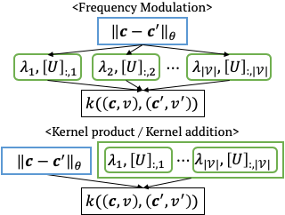
Figure 1: Influence on eigencomponents

3.1 Frequency Regularization of FM kernels

In (Smola and Kondor, 2003), it is shown that Eq. (1) defines a kernel that regularizes the eigenfunctions with high frequencies when $f$ is positive and decreasing. It is also shown that the reciprocal of $f$ in Eq. (1) is a corresponding regularization operator. For example, the diffusion kernel defined with $f(\lambda)=\exp(-\beta\lambda)$ corresponds to the regularization operator $r(\lambda)=\exp(\beta\lambda)$. The regularized Laplacian kernel defined with $f(\lambda)=1/(1+\beta\lambda)$ corresponds to the regularization operator $r(\lambda)=1+\beta\lambda$. Both regularization operators put more penalty on higher frequencies $\lambda$.

Therefore, the property FM-P1 forces FM kernels to have the same regularization effect of promoting a smoother function by penalizing the eigenfunctions with high frequencies.

3.2 Positive Definiteness of FM kernels

Determining whether Eq.3 defines a positive definite kernel is not trivial. The reason is that the gram matrix $[k((\operatorname{\mathbf{c}}_{i},v_{i}),(\operatorname{\mathbf{c}}_{j},v_{j}))]_{i,j}$ is not determined only by the entries $v_{i}$ and $v_{j}$, but these entries are additionally affected by different distance terms $\|\operatorname{\mathbf{c}}_{i}-\operatorname{\mathbf{c}}_{j}\|_{\operatorname{\mathbf{\theta}}}$. To show that FM kernels are positive definite, it is sufficient to show that $f(\lambda_{i},\|\operatorname{\mathbf{c}}-\operatorname{\mathbf{c}}^{\prime}\|_{\operatorname{\mathbf{\theta}}}|\leavevmode\nobreak\ \beta)$ is positive definite on $(\operatorname{\mathbf{c}},\operatorname{\mathbf{c}}^{\prime})\in\operatorname{\mathbb{R}}^{D_{\operatorname{\mathcal{C}}}}\times\operatorname{\mathbb{R}}^{D_{\operatorname{\mathcal{C}}}}$.

Theorem 3.1.

If $f(\lambda,\|\operatorname{\mathbf{c}}-\operatorname{\mathbf{c}}^{\prime}\|_{\operatorname{\mathbf{\theta}}}|\leavevmode\nobreak\ \beta)$ defines a positive definite kernel with respect to $\operatorname{\mathbf{c}}$ and $\operatorname{\mathbf{c}}^{\prime}$, then the FM kernel with such $f$ is positive definite jointly on $\operatorname{\mathbf{c}}$ and $v$. That is, the positive definiteness of $f(\lambda,\|\operatorname{\mathbf{c}}-\operatorname{\mathbf{c}}^{\prime}\|_{\operatorname{\mathbf{\theta}}}|\leavevmode\nobreak\ \beta)$ on $\operatorname{\mathbb{R}}^{D_{\operatorname{\mathcal{C}}}}$ implies the positive definiteness of the FM kernel on $\operatorname{\mathbb{R}}^{D_{\operatorname{\mathcal{C}}}}\times\operatorname{\mathcal{V}}$.

Proof.

See Supp. Sec.1, Thm. 1.1. ∎

Note that Theorem 3.1 shows that the property FM-P2 guarantees that FMs kernels are positive definite jointly on $\operatorname{\mathbf{c}}$ and $v$.

In the current form of Theorem 3.1, the frequency modulating functions depend on the distance $\|\operatorname{\mathbf{c}}-\operatorname{\mathbf{c}}^{\prime}\|_{\operatorname{\mathbf{\theta}}}$. However, the proof does not change for the more general form of $f(\lambda,\operatorname{\mathbf{c}},\operatorname{\mathbf{c}}^{\prime}|\alpha,\beta)$, where $f$ does not depend on $\|\operatorname{\mathbf{c}}-\operatorname{\mathbf{c}}^{\prime}\|_{\operatorname{\mathbf{\theta}}}$. Hence, Theorem 3.1 can be extended to the more general case that $f(\lambda,\operatorname{\mathbf{c}},\operatorname{\mathbf{c}}^{\prime}|\alpha,\beta)$ is positive definite on $(\operatorname{\mathbf{c}},\operatorname{\mathbf{c}}^{\prime})\in\operatorname{\mathbb{R}}^{D_{\operatorname{\mathcal{C}}}}\times\operatorname{\mathbb{R}}^{D_{\operatorname{\mathcal{C}}}}$.

3.3 Frequency Modulation Principle

A kernel, as a similarity measure, is expected to return higher values for pairs of more similar points and vice versa (Vert et al., 2004). We call such behavior the similarity measure behavior.

In Eq. (3), the distance $\|\operatorname{\mathbf{c}}-\operatorname{\mathbf{c}}^{\prime}\|_{\operatorname{\mathbf{\theta}}}$ represents a quantity in the “spatial” domain interacting with quantities $\lambda_{i}$s in the “frequency” domain. Due to the interplay between the two different domains, the kernels of the form Eq. (3) do not exhibit the similarity measure behavior for an arbitrary function $f$. Next, we derive a sufficient condition on $f$ for the similarity measure behavior to hold for FM kernels.

Formally, the similarity measure behavior is stated as

$$\|\operatorname{\mathbf{c}}-\operatorname{\mathbf{c}}^{\prime}\|_{\operatorname{\mathbf{\theta}}}\leq\|\tilde{\operatorname{\mathbf{c}}}-\tilde{\operatorname{\mathbf{c}}}^{\prime}\|_{\operatorname{\mathbf{\theta}}}$$

$$\leavevmode\nobreak\ \leavevmode\nobreak\ \Rightarrow\leavevmode\nobreak\ \leavevmode\nobreak\ k((\operatorname{\mathbf{c}},v),(\operatorname{\mathbf{c}}^{\prime},v^{\prime}))\geq k((\tilde{\operatorname{\mathbf{c}}},v),(\tilde{\operatorname{\mathbf{c}}}^{\prime},v^{\prime}))$$ (3)

or equivalently,

$$\|\operatorname{\mathbf{c}}-\operatorname{\mathbf{c}}^{\prime}\|_{\operatorname{\mathbf{\theta}}}\leq\|\tilde{\operatorname{\mathbf{c}}}-\tilde{\operatorname{\mathbf{c}}}^{\prime}\|_{\operatorname{\mathbf{\theta}}}$$

$$\leavevmode\nobreak\ \leavevmode\nobreak\ \Rightarrow\leavevmode\nobreak\ \leavevmode\nobreak\ \sum_{i=1}^{|\operatorname{\mathcal{V}}|}[U]_{v,i}h_{t_{1},t_{2}}(\lambda_{i}|\beta)[U]_{v^{\prime},i}\geq 0$$ (4)

where $h_{t_{1},t_{2}}(\lambda|\beta)=f(\lambda,t_{1}|\beta)-f(\lambda,t_{2}|\beta)$, $t_{1}=\|\operatorname{\mathbf{c}}-\operatorname{\mathbf{c}}^{\prime}\|_{\operatorname{\mathbf{\theta}}}$ and $t_{2}=\|\tilde{\operatorname{\mathbf{c}}}-\tilde{\operatorname{\mathbf{c}}}^{\prime}\|_{\operatorname{\mathbf{\theta}}}$.

Theorem 3.2.

For a connected and weighted undirected graph $\operatorname{\mathcal{G}}=(\operatorname{\mathcal{V}},\operatorname{\mathcal{E}})$ with non-negative weights on edges, define a similarity (or kernel) $a(v,v^{\prime})=[Uh(\Lambda)U^{T}]_{v,v^{\prime}}$, where $U$ and $\Lambda$ are eigenvectors and eigenvalues of the graph Laplacian $L(\operatorname{\mathcal{G}})=U\Lambda U^{T}$. If $h$ is any non-negative and strictly decreasing convex function on $[0,\infty)$, then $a(v,v^{\prime})\geq 0$ for all $v,v^{\prime}\in\operatorname{\mathcal{V}}$.

Therefore, these conditions on $h(\Lambda)$ result in a similarity measure $a$ with only positive entries, which in turn proves property Eq. (3.3). Here, we provide a proof of the theorem for a simpler case with an unweighted complete graph, where Eq. (3.3) holds without the convexity condition on $h$.

Proof.

For a unweighted complete graph with $n$ vertices, we have eigenvalues $\lambda_{1}=0$, $\lambda_{2}=\cdots=\lambda_{n}=n$ and eigenvectors such that $[U]_{\cdot 1}=1/\sqrt{n}$ and $\sum_{i=1}^{n}[U]_{v,i}[U]_{v^{\prime},i}=\delta_{vv^{\prime}}$. For $v\neq v^{\prime}$, the conclusion in Eq. (3.3), $\sum_{i=1}^{n}h(\lambda_{i})[U]_{v,i}[U]_{v^{\prime},i}$ becomes $h(0)/n+h(n)\sum_{i=2}^{n}[U]_{v,i}[U]_{v^{\prime},i}=(h(0)-h(n))/n$ in which non-negativity follows with decreasing $h$.

For the complete proof, see Thm. 2.1 in Supp. Sec. 2. ∎

Theorem 3.2 thus shows that the property FM-P3 is sufficient for Eq. (3.3) to hold. We call the property FM-P3 the frequency modulation principle. Theorem 3.2 also implies the non-negativity of many kernels derived from graph Laplacian.

Corollary 3.2.1.

The random walk kernel derived from the symmetric normalized Laplacian (Smola and Kondor, 2003), the diffusion kernels (Kondor and Lafferty, 2002; Oh et al., 2019) and the regularized Laplacian kernel (Smola and Kondor, 2003) derived from symmetric normalized or unnormalized Laplacian, are all non-negatived valued.

Proof.

See Cor. 2.1.1 in Supp. Sec. 2. ∎

3.4 FM kernels in practice

Scalability

Since the (graph Fourier) frequencies and basis functions are computed by the eigendecomposition of cubic computational complexity, a plain application of frequency modulation makes the computation of FM kernels prohibitive for a large number of discrete variables. Given $P$ discrete variables where each variable can be individually represented by a graph $\operatorname{\mathcal{G}}_{p}$, the discrete part of the search space can be represented as a product space, $\operatorname{\mathcal{V}}=\operatorname{\mathcal{V}}_{1}\times\cdots\times\operatorname{\mathcal{V}}_{P}$.

In this case, we define FM kernels on $\operatorname{\mathbb{R}}^{D_{\operatorname{\mathcal{C}}}}\times\operatorname{\mathcal{V}}=\operatorname{\mathbb{R}}^{D_{\operatorname{\mathcal{C}}}}\times(\operatorname{\mathcal{V}}_{1}\times\cdots\times\operatorname{\mathcal{V}}_{P})$ as

$$k((\operatorname{\mathbf{c}},\operatorname{\mathbf{v}}),(\operatorname{\mathbf{c}}^{\prime},\operatorname{\mathbf{v}}^{\prime})|\operatorname{\mathbf{\alpha}},\operatorname{\mathbf{\beta}},\operatorname{\mathbf{\theta}})=\prod_{p=1}^{P}k_{p}((\operatorname{\mathbf{c}},v_{p}),(\operatorname{\mathbf{c}}^{\prime},v_{p}^{\prime})|\beta_{p},\operatorname{\mathbf{\theta}})$$

$$=\prod_{p=1}^{P}\sum_{i=1}^{|\operatorname{\mathcal{V}}_{p}|}[U^{p}]_{v_{p},i}f(\lambda_{i}^{p},\alpha_{p}\|\operatorname{\mathbf{c}}-\operatorname{\mathbf{c}}^{\prime}\|_{\operatorname{\mathbf{\theta}}}|\beta_{p})[U^{p}]_{v_{p}^{\prime},i}$$ (5)

where $\operatorname{\mathbf{v}}=(v_{1},\cdots,v_{P}$, $\operatorname{\mathbf{v}}^{\prime}=(v_{1}^{\prime},\cdots,v_{P}^{\prime}$, $\operatorname{\mathbf{\alpha}}=(\alpha_{1},\cdots,\alpha_{P})$ $\operatorname{\mathbf{\beta}}=(\beta_{1},\cdots,\beta_{P})$ and the graph Laplacian is given as $L(\operatorname{\mathcal{G}}_{p})$ with the eigendecomposition $U_{p}\text{diag}[\lambda_{1}^{p},\cdots,\lambda_{\|\operatorname{\mathcal{V}}_{p}\|}^{p}]U_{p}^{T}$.

Eq.3.4 should not be confused with the kernel product of kernels on each $\operatorname{\mathcal{V}}_{p}$. Note that the distance $\|\operatorname{\mathbf{c}}-\operatorname{\mathbf{c}}^{\prime}\|_{\operatorname{\mathbf{\theta}}}$ is shared, which introduces the coupling among discrete variables and thus allows more modeling freedom than a product kernel. In addition to the coupling, the kernel parameter $\alpha_{p}$s lets us individually determine the strength of the frequency modulation.

Examples

Defining a FM kernel amounts to constructing a frequency modulating function. We introduce examples of flexible families of frequency modulating functions.

Proposition 1.

For $S\in(0,\infty)$, a finite measure $\mu$ on $[0,S]$, $\mu$-measurable $\tau:[0,S]\Rightarrow[0,2]$ and $\mu$-measurable $\rho:[0,S]\Rightarrow\operatorname{\mathbb{N}}$, the function of the form below is a frequency modulating function.

$$f(\lambda,\alpha\|\operatorname{\mathbf{c}}-\operatorname{\mathbf{c}}^{\prime}\|_{\operatorname{\mathbf{\theta}}}|\beta)$$

$$=\int_{0}^{S}\frac{1}{(1+\beta\lambda+\alpha\|\operatorname{\mathbf{c}}-\operatorname{\mathbf{c}}^{\prime}\|_{\operatorname{\mathbf{\theta}}}^{\tau(s)})^{\rho(s)}}\mu(ds)$$ (6)

Proof.

See Supp. Sec.3, Prop.2. ∎

Assuming $S=1$ and $\tau(s)=2$, Prop. 1 gives $(1+\beta\lambda+\alpha\|\operatorname{\mathbf{c}}-\operatorname{\mathbf{c}}^{\prime}\|_{\operatorname{\mathbf{\theta}}}^{2})^{-1}$ with $\rho(s)=1$ and $\mu(ds)=ds$, and $\sum_{n=1}^{N}a_{n}(1+\beta\lambda+\alpha\|\operatorname{\mathbf{c}}-\operatorname{\mathbf{c}}^{\prime}\|_{\operatorname{\mathbf{\theta}}}^{2})^{-n}$ with $\rho(s)=\lfloor Ns\rfloor$ and $\mu(\{n/N\})=a_{n}\geq 0$ and $\mu([\{n/N\}_{n=1,\cdots,N}^{c})=0$.

3.5 Extension of the Frequency Modulation

Frequency modulation is not restricted to distances on Euclidean spaces but it is applicable to any arbitrary space with a kernel defined on it. As a concrete example of frequency modulation by kernels, we show a non-stationary extension where $f$ does not depend on $\|\operatorname{\mathbf{c}}-\operatorname{\mathbf{c}}^{\prime}\|_{\operatorname{\mathbf{\theta}}}$ but on the neural network kernel $k_{NN}$ (Rasmussen, 2003). Consider Eq. (3) with $f=f_{NN}$ as follows.

$$f_{NN}(\lambda,k_{NN}(\operatorname{\mathbf{c}},\operatorname{\mathbf{c}}^{\prime}|\Sigma)|\beta)=\frac{1}{2+\beta\lambda-k_{NN}(\operatorname{\mathbf{c}},\operatorname{\mathbf{c}}^{\prime}|\Sigma)}$$ (7)

where $k_{NN}(\operatorname{\mathbf{c}},\operatorname{\mathbf{c}}^{\prime}|\Sigma)=\frac{2}{\pi}\arcsin{\Big{(}\frac{2\operatorname{\mathbf{c}}^{T}\Sigma\operatorname{\mathbf{c}}^{\prime}}{(1+\operatorname{\mathbf{c}}^{T}\Sigma\operatorname{\mathbf{c}})(1+\operatorname{\mathbf{c}}^{\prime T}\Sigma\operatorname{\mathbf{c}}^{\prime})}\Big{)}}$ is the neural network kernel (Rasmussen, 2003).

Since the range of $k_{NN}$ is $[-1,1]$, $f_{NN}$ is positive and thus satisfies FM-P1. Through Eq.7, Eq.3 is positive definite (Supp. Sec.3, Prop.3) and thus property FM-P2 is satisfied. If the premise $t_{1}<t_{2}$ of the property FM-P3 is replaced by $t_{1}>t_{2}$, then FM-P3 is also satisfied. In contrast to the frequency modulation principle with distances in Eq. (3.3), the frequency modulation principle with a kernel is formalized as

$$k_{NN}(\operatorname{\mathbf{c}},\operatorname{\mathbf{c}}^{\prime}|\Sigma)\geq k_{NN}(\tilde{\operatorname{\mathbf{c}}},\tilde{\operatorname{\mathbf{c}}}^{\prime}|\Sigma)$$

$$\Rightarrow k((\operatorname{\mathbf{c}},v),(\operatorname{\mathbf{c}}^{\prime},v^{\prime}))\geq k((\tilde{\operatorname{\mathbf{c}}},v),(\tilde{\operatorname{\mathbf{c}}}^{\prime},v^{\prime}))$$ (8)

Note that $k_{NN}(\operatorname{\mathbf{c}},\operatorname{\mathbf{c}}^{\prime}|\Sigma)$ is a similarity measure and thus the inequality is not reversed unlike Eq. (3.3).

All above arguments on the extension of the frequency modulation using a nonstationary kernel hold also when the $k_{NN}$ is replaced by an arbitrary positive definite kernel. The only required condition is that a kernel has to be upper bounded, i.e., $k_{NN}(\operatorname{\mathbf{c}},\operatorname{\mathbf{c}}^{\prime})\leq C$, needed for FM-P1 and FM-P2.

4 Related work

On continuous variables, many sophisticated kernels have been proposed (Wilson and Nickisch, 2015; Samo and Roberts, 2015; Remes et al., 2017; Oh et al., 2018). In contrast, kernels on discrete variables have been studied less (Haussler, 1999; Kondor and Lafferty, 2002; Smola and Kondor, 2003). To our best knowledge, most of existing kernels on mixed variables are constructed by a kernel product Swersky et al. (2013); Li et al. (2016) with some exceptions (Krause and Ong, 2011; Swersky et al., 2013; Fiducioso et al., 2019), which rely on kernel addition.

In mixed variable BO, non-GP surrogate models are more prevalent, including SMAC (Hutter et al., 2011) using random forest and TPE (Bergstra et al., 2011) using a tree structured density estimator. Recently, by extending the approach of using Bayesian linear regression for discrete variables (Baptista and Poloczek, 2018), Daxberger et al. (2019) proposes Bayesian linear regression with manually chosen basis functions on mixed variables, providing a regret analysis using Thompson sampling as an acquisition function. Another family of approaches utilizes a bandit framework to handle the acquisition function optimization on mixed variables with theoretical analysis (Gopakumar et al., 2018; Nguyen et al., 2019; Ru et al., 2020). Nguyen et al. (2019) use GP in combination with multi-armed bandit to model category-specific continuous variables and provide regret analysis using GP-UCB. Among these approaches, Ru et al. (2020) also utilize information across different categorical values, which –in combination with the bandit framework– makes itself the most competitive method in the family.

Our focus is to extend the modelling prowess and flexibility of pure GPs for surrogate models on problems with mixed variables. We propose frequency modulated kernels, which are kernels that are specifically designed to model the complex interactions between continuous and discrete variables.

In architecture search, approaches using weight sharing such as DARTS (Liu et al., 2018) and ENAS (Pham et al., 2018) are gaining popularity. In spite of their efficiency, methods training neural networks from scratch for given architectures outperform approaches based on weight sharing (Dong et al., 2021). Moreover, the joint optimization of learning hyperparameters and architectures is under-explored with a few exceptions such as BOHB (Falkner et al., 2018) and autoHAS (Dong et al., 2020). Our approach proposes a competitive option to this challenging optimization of mixed variable functions with expensive evaluation cost.

5 Experiments

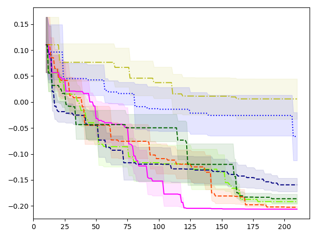
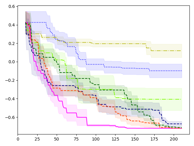
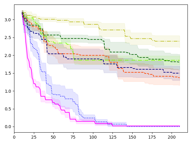
	SMAC	TPE	ModDif	ModLap	CoCaBO-0.0	CoCaBO-0.5	CoCaBO-1.0
Func2C	$+0.006\pm 0.039$	$-0.192\pm 0.005$	$-0.066\pm 0.046$	$\mathbf{-0.206\pm 0.000}$	$-0.159\pm 0.013$	$\mathit{-0.202\pm 0.002}$	$-0.186\pm 0.009$
Func3C	$+0.119\pm 0.072$	$-0.407\pm 0.120$	$-0.098\pm 0.074$	$\mathbf{-0.722\pm 0.000}$	$-0.673\pm 0.027$	$\mathit{-0.720\pm 0.002}$	$-0.714\pm 0.005$
Ackley5C	$+2.381\pm 0.165$	$+1.860\pm 0.125$	$\mathbf{+0.001\pm 0.000}$	$\mathit{+0.019\pm 0.006}$	$+1.499\pm 0.201$	$+1.372\pm 0.211$	$+1.811\pm 0.217$

Figure 2: Func2C(left), Func3C(middle), Ackley5C(right) (Mean$\pm$Std.Err. of 5 runs)

To demonstrate the improved sample efficiency of GP BO using FM kernels (BO-FM) we study various mixed variable black-box function optimization tasks, including 3 synthetic problems from Ru et al. (2020), 2 hyperparameter optimization problems (SVM (Smola and Kondor, 2003) and XGBoost (Chen and Guestrin, 2016)) and the joint optimization of neural architecture and SGD hyperparameters.

As per our method, we consider ModLap which is of the form Eq. 3.4 with the following frequency modulating function.

$$f_{Lap}(\lambda,\|\operatorname{\mathbf{c}}-\operatorname{\mathbf{c}}^{\prime}\|_{\operatorname{\mathbf{\theta}}}|\alpha,\beta)=\frac{1}{1+\beta\lambda+\alpha\|\operatorname{\mathbf{c}}-\operatorname{\mathbf{c}}^{\prime}\|_{\operatorname{\mathbf{\theta}}}^{2}}$$ (9)

Moreover, to empirically demonstrate the importance of the similarity measure behavior, we consider another kernel following the form of Eq. 3.4 but disrespecting the frequency modulation principle with the function

$$f_{Dif}(\lambda,\|\operatorname{\mathbf{c}}-\operatorname{\mathbf{c}}^{\prime}\|_{\operatorname{\mathbf{\theta}}}|\alpha,\beta)=\exp{(-(1+\alpha\|\operatorname{\mathbf{c}}-\operatorname{\mathbf{c}}^{\prime}\|_{\operatorname{\mathbf{\theta}}}^{2})\beta\lambda)}$$ (10)

We call the kernel constructed with this function ModDif. The implementation of these kernels is publicly available.

In each round, after updating with an evaluation, we fit a GP surrogate model using marginal likelihood maximization with 10 random initialization until convergence (Rasmussen, 2003). We use the expected improvement (EI) acquisition function (Donald, 1998) and optimize it by repeated alternation of L-BFGS-B (Zhu et al., 1997) and hill climbing (Skiena, 1998) until convergence. More details on the experiments are provided in Supp. Sec. 4.

Baselines

For synthetic problems and hyperparameter optimization problems below, baselines we consider are SMAC (Hutter et al., 2011), TPE (Bergstra et al., 2011), and CoCaBO (Ru et al., 2020) which consistently outperforms One-hot BO (authors, 2016) and EXP3BO (Gopakumar et al., 2018). For CoCaBO, we consider 3 variants using different mixture weights.

5.1 Synthetic problems

We test on 3 synthetic problems proposed in Ru et al. (2020). Each of the synthetic problems has the search space as in Tab. 1. Details of synthetic problems can be found in Ru et al. (2020).

	Conti. Space	Num. of Cats.
Func2C	$[-1,1]^{2}$	3, 5
Func3C	$[-1,1]^{2}$	3, 5,4
Ackley5C	$[-1,1]$	17, 17, 17, 17, 17

Table 1: Synthetic Problem Search Spaces

On all 3 synthetic benchmarks, ModLap shows competitive performance (Fig. 2). On Func2C and Func3C, ModLap performs the best, while on Ackley5C ModLap is at the second place, marginally further from the first. Notably, even on Func2C and Func3C, where ModDif underperforms significantly, ModLap exhibits its competitiveness, which empirically supports that the similarity measure behavior plays an important role in the surrogate modeling in Bayesian optimization. Note that TPE and CoCaBO have much shorter wall-clock runtime.

5.2 Hyperparameter optimization problems

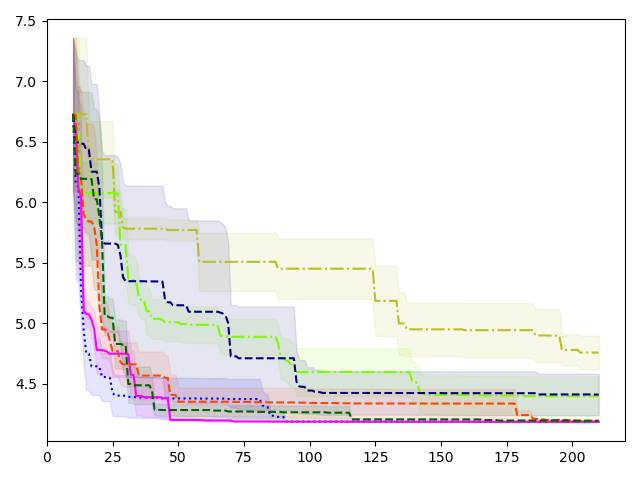
SVM	Method	XGBoost
$4.759\pm.141$	SMAC	$.1215\pm.0045$
$4.399\pm.163$	TPE	$.1084\pm.0007$
$\mathit{4.188\pm.001}$	ModDif	$\mathit{.1071\pm.0013}$
$\mathbf{4.186\pm.002}$	ModLap	$\mathbf{.1038\pm.0003}$
$4.412\pm.170$	CoCaBO-0.0	$.1184\pm.0062$
$4.196\pm.004$	CoCaBO-0.5	$.1079\pm.0010$
$4.196\pm.004$	CoCaBO-1.0	$.1086\pm.0008$

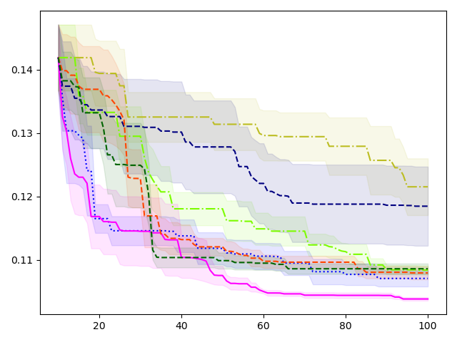
Figure 3: SVM(left), XGBoost(right) (Mean$\pm$Std.Err. of 5 runs)

Now we consider a practical application of Bayesian optimization over mixed variables. We take two machine learning algorithms, SVM (Smola and Kondor, 2003) and XGBoost (Chen and Guestrin, 2016) and optimize their hyperparameters.

SVM

We optimize hyperparameters of NuSVR in scikit-learn (Pedregosa et al., 2011). We consider 3 categorical hyperparameters and 3 continuous hyperparameters (Tab. 2) and for continuous hyperparameters we search over $\log_{10}$ transformed space of the range.

NuSVR param.	Range
kernel	$\{$linear, poly, RBF, sigmoid $\}$
gamma	$\{$scale, auto $\}$
shrinking	$\{$on, off $\}$
C	$[10^{-4},10]$
tol	$[10^{-6},1]$
nu	$[10^{-6},1]$

Table 2: NuSVR hyperparameters

For each of 5 split of Boston housing dataset with train:test(7:3) ratio, NuSVR is fitted on the train set and RMSE on the test set is computed. The average of 5 test RMSE is the objective.

XGBoost

We consider 1 ordinal, 3 categorical and 4 continuous hyperparameters (Tab. 3).

XGBoost param.	Range
max_depth	$\{1,\cdots,10\}$
booster	$\{$gbtree, dart$\}$
grow_policy	$\{$depthwise, lossguide$\}$
objective	$\{$multi:softmax, multi:softprob$\}$
eta	$[10^{-6},1]$
gamma	$[10^{-4},10]$
subsample	$[10^{-3},1]$
lambda	$[0,5]$

Table 3: XGBoost hyperparameters

For 3 continuous hyperparameters, eta, gamma and subsample, we search over the $\log_{10}$ transformed space of the range. With a stratified train:test(7:3) split, the model is trained with 50 rounds and the best test error over 50 rounds is the objective of SVM hyperparameter optimization.

In Fig. 3, ModLap performs the best. On XGBoost hyperparameter optimization, ModLap exhibits clear benefit compared to the baselines. Here, ModDif wins the second place in both problems.

Comparison to different kernel combinations

In Supp. Sec. 5, we also report the comparison with different kernel combinations on all 3 synthetic problems and 2 hyperparameter parameter optimization problems. We make two observations. First, ModDif, which does not respect the similarity measure behavior, sometimes severely degrades BO performance. Second, ModLap obtains equally good final results and consistently finds the better solutions faster than the kernel product. This can be clearly shown by comparing the area above the mean curve of BO runs using different kernels. The area above the mean curve of BO using ModLap is larger than the are above the mean curve of BO using the kernel product. Moreover, the gap between the area from ModLap and the area from kernel product increases in problems with larger search spaces. Even on the smallest search space, Func2C, ModLap lags behind the kernel product up to around 90th evaluation and outperforms after it. The benefit of ModLap modeling complex dependency among mixed variables is more prominent in higher dimension problems.

Ablation study on regression tasks

In addition to the results on BO experiments, we compare FM kernels with kernel addiition and kernel product on three regression tasks from UCI datasets (Supp. Sec. 6). In terms of negative log-likelihood (NLL), which takes into account uncertainty, ModLap performs the best in two out of three tasks. Even on the task which is conjectured to have a structure suitable to kernel product, ModLap shows competitive performance. Moreover, on regression tasks, the importance of the frequency modulation principle is further reinforced. For full NLL and RMSE comparison and detailed discussion, see Supp. Sec. 6

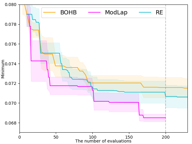
Method	#Eval.	Mean$\pm$Std.Err.
BOHB	200	$7.158\text{\times}{10}^{-02}$$\pm$$1.0303\text{\times}{10}^{-03}$
BOHB	230	$7.151\text{\times}{10}^{-02}$$\pm$$9.8367\text{\times}{10}^{-04}$
BOHB	600	$6.941\text{\times}{10}^{-02}$$\pm$$4.4320\text{\times}{10}^{-04}$
RE	200	$7.067\text{\times}{10}^{-02}$$\pm$$1.1417\text{\times}{10}^{-03}$
RE	230	$7.061\text{\times}{10}^{-02}$$\pm$$1.1329\text{\times}{10}^{-03}$
RE	400	$6.929\text{\times}{10}^{-02}$$\pm$$6.4804\text{\times}{10}^{-04}$
RE	600	$6.879\text{\times}{10}^{-02}$$\pm$$1.0039\text{\times}{10}^{-03}$
ModLap	200	$6.850\text{\times}{10}^{-02}$$\pm$$3.7914\text{\times}{10}^{-04}$

For the figure with all numbers above, see Supp. Sec. 5.

Figure 4: Joint optimization of the architecture and SGD hyperparameters (Mean$\pm$Std.Err. of 4 runs)

5.3 Joint optimization of neural architecture and SGD hyperparameters

Next, we experiment with BO on mixed variables by optimizing continuous and discrete hyperparameters of neural networks. The space of discrete hyperparameters $\mathcal{A}$ is modified from the NASNet search space (Zoph and Le, 2016), which consists of 8,153,726,976 choices. The space of continuous hyperparameters $\mathcal{H}$ comprises 6 continuous hyperparameters of the SGD with a learning rate scheduler: learning rate, momentum, weight decay, learning rate reduction factor, 1st reduction point ratio and 2nd reduction point ratio. A good neural architecture should both achieve low errors and be computationally modest. Thus, we optimize the objective $f(a,h)=err_{valid}(a,h)+0.02\times FLOP(a)/\max_{a^{\prime}\in\mathcal{A}}FLOP(a^{\prime})$. To increase the separability among smaller values, we use $\log f(a,h)$ transformed values whenever model fitting is performed on evaluation data. The reported results are still the original non-transformed $f(a,h)$.

We compare with two strong baselines. One is BOHB (Falkner et al., 2018) which is an evaluation-cost-aware algorithm augmenting unstructured bandit approach (Li et al., 2017) with model-based guidance. Another is RE (Real et al., 2019) based on a genetic algorithm with a novel population selection strategy. In Dong et al. (2021), on discrete-only spaces, these two outperform competitors including weight sharing approaches such as DARTS (Liu et al., 2018), SETN (Dong and Yang, 2019), ENAS (Pham et al., 2018) and etc. In the experiment, for BOHB, we use the public implementation and for RE, we use our own implementation.

For a given set of hyperparameters, with ModLap or RE, the neural network is trained on FashionMNIST for 25 epochs while BOHB adaptively chooses the number of epochs. For further details on the setup and the baselines we refer the reader to Supp. Sec. 4 and 5.

We present the results in Fig. 4. Since BOHB adaptively chooses the budget (the number of epochs), BOHB is plotted according to the budget consumption. For example, the y-axis value of BOHB on 100-th evaluation is the result of BOHB having consumed 2,500 epochs (25 epochs $\times$ 100).

We observe that ModLap finds the best architecture in terms of accuracy and computational cost. What is more, we observe that ModLap reaches the better solutions faster in terms of numbers of evaluations. Even though the time to evaluate a new hyperparameter is dominant, the time to suggest a new hyperparameter in ModLap is not negligible in this case. Therefore, we also provide the comparison with respect the wall-clock time. It is estimated that RE and BOHB evaluate 230 hyperparameters while ModLap evaluate 200 hyperparameters (Supp. Sec. 4). For the same estimated wall-clock time, ModLap(200) outperforms competitors(RE(230), BOHB(230)).

In order to see how beneficial the sample efficiency of BO-FM is in comparison to the baselines, we perform a stress test in which more evaluations are allowed for RE and BOHB. We leave RE and BOHB for 600 evaluations. Notably, ModLap with 200 evaluations outperforms both competitors with 600 evaluations (Fig. 4 and Supp.Sec. 5). We conclude that ModLap exhibits higher sample efficiency than the baselines.

6 Conclusion

We propose FM kernels to improve the sample efficiency of mixed variable Bayesian optimization.

On the theoretical side, we provide and prove conditions for FM kernels to be positive definite and to satisfy the similarity measure behavior. Both conditions are not trivial due to the interactions between quantities on two disparate domains, the spatial domain and the frequency domain.

On the empirical side, we validate the effect of the conditions for FM kernels on multiple synthetic problems and realistic hyperparameter optimization problems. Further, we successfully demonstrate the benefits of FM kernels compared to non-GP based Bayesian Optimization on a challenging joint optimization of neural architectures and SGD hyperparameters. BO-FM outperforms its competitors, including Regularized evolution, which requires three times as many evaluations.

We conclude that an effective modeling of dependencies between different types of variables improves the sample efficiency of BO. We believe the generality of the approach can have a wider impact on modeling dependencies between discrete variables and variables of arbitrary other types, including continuous variables.

Mixed Variable Bayesian Optimization with Frequency Modulated Kernels
Supplementary Material

1 Positive definite FM kernels

For a weighted undirected graph $\operatorname{\mathcal{G}}=(\operatorname{\mathcal{V}},\operatorname{\mathcal{E}})$ with graph Laplacian $L(\operatorname{\mathcal{G}})=U\Lambda U^{T}$. Frequency modulating kernels are defined as

$$k((\operatorname{\mathbf{c}},v),(\operatorname{\mathbf{c}}^{\prime},v^{\prime})\|\operatorname{\mathbf{\theta}},\beta)=[\sum_{i=1}^{\|\operatorname{\mathcal{V}}\|}[U]_{:,i}f(\lambda_{i},\|\operatorname{\mathbf{c}}-\operatorname{\mathbf{c}}^{\prime}\|_{\operatorname{\mathbf{\theta}}}\|\beta)[U]_{:,i}]_{v,v^{\prime}}$$ (11)

where $[U]_{:,i}$ are eigenvectors of $L(\operatorname{\mathcal{G}})$ which are columns of $U$ and $\lambda_{i}=[\Lambda]_{ii}$ are corresponding eigenvalues. $\operatorname{\mathbf{c}}$ and $\operatorname{\mathbf{c}}^{\prime}$ are continuous variables in $\operatorname{\mathbb{R}}^{D_{\operatorname{\mathcal{C}}}}$, $\operatorname{\mathbf{\theta}}\in\operatorname{\mathbb{R}}^{D_{\operatorname{\mathcal{C}}}}$ is a kernel parameter similar to the lengthscales in the RBF kernel. $\beta\in\operatorname{\mathbb{R}}$ is a kernel parameter from kernels derived from the graph Laplacian.

Theorem 1.1.

If $f(\lambda,\|\operatorname{\mathbf{c}}-\operatorname{\mathbf{c}}^{\prime}\|_{\operatorname{\mathbf{\theta}}}\|\beta)$ defines a positive definite kernel on $(\operatorname{\mathbf{c}},\operatorname{\mathbf{c}}^{\prime})\in\operatorname{\mathbb{R}}^{D_{\operatorname{\mathcal{C}}}}\times\operatorname{\mathbb{R}}^{D_{\operatorname{\mathcal{C}}}}$, then a FreMod kernel defined with such $f$ is positive definite jointly on $(\operatorname{\mathbf{c}},v)$.

Proof.

$$\small k((\operatorname{\mathbf{c}},v),(\operatorname{\mathbf{c}}^{\prime},v^{\prime})\|\operatorname{\mathbf{\theta}},\beta)=\Big{[}\sum_{i=1}^{\|\operatorname{\mathcal{V}}\|}[U]_{:,i}f(\lambda_{i},\|\operatorname{\mathbf{c}}-\operatorname{\mathbf{c}}^{\prime}\|_{\operatorname{\mathbf{\theta}}}\|\beta)[U]_{:,i}\Big{]}_{v,v^{\prime}}=\sum_{i=1}^{\|\operatorname{\mathcal{V}}\|}[U]_{v,i}f(\lambda_{i},\|\operatorname{\mathbf{c}}-\operatorname{\mathbf{c}}^{\prime}\|_{\operatorname{\mathbf{\theta}}}\|\beta)[U]_{v^{\prime},i}$$ (12)

Since a sum of positive definite(PD) kernels is PD, we prove PD of frequency modulating kernels by showing that $k_{i}((\operatorname{\mathbf{c}},v),(\operatorname{\mathbf{c}}^{\prime},v^{\prime})\|\operatorname{\mathbf{\theta}},\beta)=[U]_{v,i}f(\lambda_{i},\|\operatorname{\mathbf{c}}-\operatorname{\mathbf{c}}^{\prime}\|_{\operatorname{\mathbf{\theta}}}\|\beta)[U]_{v^{\prime},i}$ is PD.

Let us consider $\operatorname{\mathbf{a}}\in\operatorname{\mathbb{R}}^{S}$, $\mathcal{D}=\{(\operatorname{\mathbf{c}}_{1},v_{1}),\cdots,(\operatorname{\mathbf{c}}_{S},v_{S})\}$, then

$$\operatorname{\mathbf{a}}^{T}\begin{bmatrix}[U]_{v_{1},i}f(\lambda_{i},\|\operatorname{\mathbf{c}}_{1}-\operatorname{\mathbf{c}}_{1}\|_{\operatorname{\mathbf{\theta}}}|\beta)[U]_{v_{1},i}&\cdots&[U]_{v_{1},i}f(\lambda_{i},\|\operatorname{\mathbf{c}}_{1}-\operatorname{\mathbf{c}}_{S}\|_{\operatorname{\mathbf{\theta}}}|\beta)[U]_{v_{S},i}\\ [U]_{v_{2},i}f(\lambda_{i},\|\operatorname{\mathbf{c}}_{2}-\operatorname{\mathbf{c}}_{1}\|_{\operatorname{\mathbf{\theta}}}|\beta)[U]_{v_{1},i}&\cdots&[U]_{v_{2},i}f(\lambda_{i},\|\operatorname{\mathbf{c}}_{2}-\operatorname{\mathbf{c}}_{S}\|_{\operatorname{\mathbf{\theta}}}|\beta)[U]_{v_{S},i}\\ \vdots&\cdots&\vdots\\ [U]_{v_{S},i}f(\lambda_{i},\|\operatorname{\mathbf{c}}_{S}-\operatorname{\mathbf{c}}_{1}\|_{\operatorname{\mathbf{\theta}}}|\beta)[U]_{v_{1},i}&\cdots&[U]_{v_{S},i}f(\lambda_{i},\|\operatorname{\mathbf{c}}_{S}-\operatorname{\mathbf{c}}_{S}\|_{\operatorname{\mathbf{\theta}}}|\beta)[U]_{v_{S},i}\end{bmatrix}\operatorname{\mathbf{a}}$$

$$=(\operatorname{\mathbf{a}}\circ[U]_{:,i})^{T}\begin{bmatrix}f(\lambda_{i},\|\operatorname{\mathbf{c}}_{1}-\operatorname{\mathbf{c}}_{1}\|_{\operatorname{\mathbf{\theta}}}\|\beta)&\cdots&f(\beta\lambda_{i},\|\operatorname{\mathbf{c}}_{1}-\operatorname{\mathbf{c}}_{S}\|_{\operatorname{\mathbf{\theta}}}|\beta)\\ f(\lambda_{i},\|\operatorname{\mathbf{c}}_{2}-\operatorname{\mathbf{c}}_{1}\|_{\operatorname{\mathbf{\theta}}}\|\beta)&\cdots&f(\beta\lambda_{i},\|\operatorname{\mathbf{c}}_{2}-\operatorname{\mathbf{c}}_{S}\|_{\operatorname{\mathbf{\theta}}}|\beta)\\ \vdots&\cdots&\vdots\\ f(\lambda_{i},\|\operatorname{\mathbf{c}}_{S}-\operatorname{\mathbf{c}}_{1}\|_{\operatorname{\mathbf{\theta}}}\|\beta)&\cdots&f(\beta\lambda_{i},\|\operatorname{\mathbf{c}}_{S}-\operatorname{\mathbf{c}}_{S}\|_{\operatorname{\mathbf{\theta}}}|\beta)\end{bmatrix}(\operatorname{\mathbf{a}}\circ[U]_{:,i})$$ (13)

where $\circ$ is Hadamard(elementwise) product and $[U]_{:,i}=[[U]_{v_{1},i},\cdots,[U]_{v_{S},i}]^{T}$.

By letting $\operatorname{\mathbf{a}}^{\prime}=\operatorname{\mathbf{a}}\circ[U_{i}]_{\pi_{i}(v_{:}),n}$, since $f(\lambda_{i},\|\operatorname{\mathbf{c}}-\operatorname{\mathbf{c}}^{\prime}\|_{\operatorname{\mathbf{\theta}}}\|\beta)$ is PD, we show that $k_{i}((\operatorname{\mathbf{c}},v),(\operatorname{\mathbf{c}}^{\prime},v^{\prime})\|\operatorname{\mathbf{\theta}},\beta)=u_{i,v}f(\lambda_{i},\|\operatorname{\mathbf{c}}-\operatorname{\mathbf{c}}^{\prime}\|_{\operatorname{\mathbf{\theta}}}\|\beta)u_{i,v^{\prime}}$ is PD. ∎

2 Nonnegative valued FM kernels

Theorem 2.1.

For a connected and undirected graph $\operatorname{\mathcal{G}}=(\operatorname{\mathcal{V}},\operatorname{\mathcal{E}})$ with non-negative weights on edges, define a kernel $k(v,v^{\prime})=[Uf(\Lambda)U^{T}]_{v,v^{\prime}}$ where $U$ and $\Lambda$ are eigenvectors and eigenvalues of the graph Laplacian $L(\operatorname{\mathcal{G}})=U\Lambda U^{T}$. If $f$ is any non-negative and strictly decreasing convex function on $[0,\infty)$, then $K(v,v^{\prime})\geq 0$ for all $v,v^{\prime}\in\operatorname{\mathcal{V}}$.

Proof.

For a connected and weighted undirected graph $\operatorname{\mathcal{G}}=(\operatorname{\mathcal{V}},\operatorname{\mathcal{E}})$, the graph Laplacian $L(G)$ has exactly one $0$ eigenvalue and the corresponding eigenvector $1/\sqrt{D}[1,\cdots,1]^{T}$ when $|\operatorname{\mathcal{V}}|=D$.

We show that

$$\min_{v,v^{\prime}}k_{\operatorname{\mathcal{G}}}(v,v^{\prime})=\min_{p,q=1,\cdots,D}[Uf(\Lambda)U^{T}]_{p,q}\geq 0$$ (14)

for an arbitrary connected and weighted undirected graph $\operatorname{\mathcal{G}}=(\operatorname{\mathcal{V}},\operatorname{\mathcal{E}})$ where $|\operatorname{\mathcal{V}}|=D$ and $L(\operatorname{\mathcal{G}})=U\Lambda U^{T}$.

For a connected graph, there is only one zero eigenvalue

$$0=\lambda_{1}<\lambda_{2}\leq\cdots\leq\lambda_{D}\quad\text{where}\quad\lambda_{i}=[\Lambda]_{i,i}$$ (15)

and the corresponding eigenvector is given as

$$U_{1,q}=\frac{1}{\sqrt{D}}(q=1,\cdots,D).$$ (16)

From the definition of eigendecomposition, we have

$$U^{T}U=UU^{T}=I.$$ (17)

Importantly, from the definition of the graph Laplacian

$$[U\Lambda U^{T}]_{p,q}\leq 0\quad\text{when}\quad p\neq q.$$ (18)

For a given diagonal matrix $\Lambda$ such that $0=\lambda_{1}<\lambda_{2}\leq\cdots\leq\lambda_{D}$ where $\lambda_{i}=[\Lambda]_{i,i}$, we solve the following minimization problem

$$\min_{[U]_{p,i},[U]_{q,i}}\frac{f(0)}{D}+\sum_{i=2}^{D}f(\lambda_{i})[U]_{p,i}[U]_{q,i}$$ (19)

with the constraints

$$\sum_{i=2}^{D}\lambda_{i}[U]_{p,i}[U]_{q,i}\leq 0(p\neq q),\quad\sum_{i=2}^{D}[U]_{p,i}^{2}=\sum_{i=2}^{D}[U]_{q,i}^{2}=1-\frac{1}{D},\quad\sum_{i=2}^{D}[U]_{p,i}[U]_{q,i}=-\frac{1}{D}(p\neq q)$$ (20)

When $p=q$, eq.19 is nonnegative because $f$ is nonnegative valued. From now on, we consider the case $p\neq q$.

Lagrange multiplier is given as

$$L_{KKT}([U]_{p,i},[U]_{q,i},\eta,a,b,c) =\frac{f(0)}{D}+\sum_{i=2}^{D}f(\lambda_{i})[U]_{p,i}[U]_{q,i}+\eta\Big{(}\sum_{i=2}^{D}\lambda_{i}[U]_{p,i}[U]_{q,i}\Big{)}$$

$$+a\Big{(}\sum_{i=2}^{D}[U]_{p,i}^{2}-(1-\frac{1}{D})\Big{)} +b\Big{(}\sum_{i=2}^{D}[U]_{q,i}^{2}-(1-\frac{1}{D})\Big{)}+c\Big{(}\sum_{i=2}^{D}[U]_{p,i}[U]_{q,i}+\frac{1}{D}\Big{)}$$ (21)

with $\eta\geq 0$.

The stationary conditions are given as

$$\frac{\partial L_{KKT}}{\partial[U]_{p,i}}=f(\lambda_{i})[U]_{q,i}+\eta\lambda_{i}[U]_{q,i}+c[U]_{q,i}+2a[U]_{p,i}=0$$ (22)

$$\frac{\partial L_{KKT}}{\partial[U]_{q,i}}=f(\lambda_{i})[U]_{p,i}+\eta\lambda_{i}[U]_{p,i}+c[U]_{p,i}+2b[U]_{q,i}=0$$ (23)

from which, we have

$$(f(\lambda_{i})+\eta\lambda_{i}+c)[U]_{q,i}=-2a[U]_{p,i}$$ (24)

$$(f(\lambda_{i})+\eta\lambda_{i}+c)[U]_{p,i}=-2b[U]_{q,i}$$ (25)

By using

$$\sum_{i=2}^{D}\frac{\partial L_{KKT}}{\partial[U]_{p,i}}[U]_{p,i}=\sum_{i=2}^{D}\frac{\partial L_{KKT}}{\partial[U]_{q,i}}[U]_{q,i}=0$$ (26)

we have $a=b$.

From eq.(24) and eq.(25), we get

$$((f(\lambda_{i})+\eta\lambda_{i}+c)^{2}-4ab)[U]_{q,i}=0$$ (27)

$$((f(\lambda_{i})+\eta\lambda_{i}+c)^{2}-4ab)[U]_{p,i}=0$$ (28)

If $i\in\{i|(f(\lambda_{i})+\eta\lambda_{i}+c)^{2}-4ab\neq 0\}$, we have $[U]_{p,i}=[U]_{q,i}=0$. On the other hand, if $(f(\lambda_{i})+\eta\lambda_{i}+c)^{2}-4ab=0$, then we have $f(\lambda_{i})+\eta\lambda_{i}+c=-2a$ or $f(\lambda_{i})+\eta\lambda_{i}+c=2a$ because $a=b$.

We define three index sets

$$I_{0} =\{i|(f(\lambda_{i})+\eta\lambda_{i}+c)^{2}-4a^{2}\neq 0\}$$ (29)

$$I_{+} =\{i|f(\lambda_{i})+\eta\lambda_{i}+c+2a=0\}-\{1\}$$ (30)

$$I_{-} =\{i|f(\lambda_{i})+\eta\lambda_{i}+c-2a=0\}$$ (31)

from eq.(24) and eq.(25), we have

$$i\in I_{0} \Rightarrow[U]_{p,i}=[U]_{q,i}=0$$ (32)

$$i\in I_{+} \Rightarrow[U]_{p,i}=[U]_{q,i}$$ (33)

$$i\in I_{-} \Rightarrow[U]_{p,i}=-[U]_{q,i}$$ (34)

With these conditions, the constraints can be expressed as

$$\sum_{i_{+}\in I_{+}}\lambda_{i_{+}}[U]_{p,i}^{2}-\sum_{i_{-}\in I_{-}}\lambda_{i_{-}}[U]_{p,i}^{2}\leq 0,\quad\sum_{i_{+}\in I_{+}}[U]_{p,{i_{+}}}^{2}=\frac{1}{2}-\frac{1}{D},\quad\sum_{i_{-}\in I_{-}}[U]_{p,{i_{-}}}^{2}=\frac{1}{2}$$ (35)

We divide cases according to the number of solutions $g(\lambda)=f(\lambda)+\eta\lambda$ can have. i) $f(\lambda)+\eta\lambda$ can have at most one solution, ii) $f(\lambda)+\eta\lambda$ may have two solutions. Note that $g(\lambda)$ is convex as sum of two convex functions. Since a convex function can have at most two zeros unless it is constantly zero, these two cases are exhaustive. When $\eta=0$, $f(\lambda)$ is strictly decreasing function and, thus $g(\lambda)$ has at most one solution. Also, when $\eta\geq-f^{\prime}(0)=\max_{\lambda}-f^{\prime}(\lambda)$, $f^{\prime}(\lambda)+\eta$ is positive except for $\lambda=0$ and $g(\lambda)$ has at most one solution.

Case i)

$f(\lambda)+\eta\lambda$ can have at most one solution. ($\eta=0$ or $\eta\geq-f^{\prime}(0)=\max_{\lambda}-f^{\prime}(\lambda)$)

Let us denote $\lambda^{E}$ the unique solution of $f(\lambda_{i})+\eta\lambda_{i}+c+2a=0$ and $\lambda^{N}$ the unique of $f(\lambda_{i})+\eta\lambda_{i}+c-2a=0$.

Therefore $\lambda_{i_{+}}=\lambda^{E}$, $\forall i_{+}\in I_{+}$ and $\lambda_{i_{-}}=\lambda^{N}$, $\forall i_{-}\in I_{-}$. The minimization objective becomes

$$\frac{f(0)}{D}+\sum_{i=2}^{D}f(\lambda_{i})[U]_{p,i}[U]_{q,i} =\frac{f(0)}{D}+f(\lambda^{E})\sum_{i_{+}\in I_{+}}[U]_{p,i}^{2}-f(\lambda_{N})\sum_{i_{-}\in I_{-}}[U]_{p,i}^{2}$$

$$=\frac{f(0)}{D}+\Big{(}\frac{1}{2}-\frac{1}{D}\Big{)}f(\lambda^{E})-\frac{1}{2}f(\lambda^{N})$$ (36)

The inequality constraint becomes

$$\sum_{i=2}^{D}\lambda_{i}[U]_{p,i}[U]_{q,i}=\frac{f(0)}{D}+\lambda^{E}\sum_{i_{+}\in I_{+}}[U]_{p,i_{+}}^{2}-\lambda_{N}\sum_{i_{-}\in I_{-}}[U]_{p,i_{-}}^{2}=\Big{(}\frac{1}{2}-\frac{1}{D}\Big{)}\lambda^{E}-\frac{1}{2}\lambda^{N}\leq 0$$ (37)

Since $\lambda^{E},\lambda^{N}\in\{\lambda_{2},\cdots,\lambda_{D}\}$, there is maximum value with respect to the choice of $\lambda^{E},\lambda^{N}$. We consider continuous relaxation of the minimization problem with respect to $\lambda^{E},\lambda^{N}$. By showing that the objective is nonnegative when $\lambda^{E}\geq 0,\lambda^{N}\geq 0$, we prove our claim. When we consider continuous optimization problem over $\lambda^{E},\lambda^{N}$, the minimum is obtained when the inequality constraint becomes equality constraints. If $\Big{(}\frac{1}{2}-\frac{1}{D}\Big{)}\lambda^{E}-\frac{1}{2}\lambda^{N}<0$ by increasing $\lambda^{E}$ by $\delta>0$ so that $\Big{(}\frac{1}{2}-\frac{1}{D}\Big{)}(\lambda^{E}+\delta)-\frac{1}{2}\lambda^{N}=0$, $f(\lambda^{E})$ is decreased to $f(\lambda^{E}+\delta)$, thus the minimum is obtained when the inequality constraint is equality. When $\eta>0$, the inequality constraint automatically becomes an equality constraint by the slackness condition of the Karush-Kuhn-Tucker conditions.

With the inequality condition the objective becomes

$$\frac{f(0)}{D}+\Big{(}\frac{1}{2}-\frac{1}{D}\Big{)}f(\lambda^{E})-\frac{1}{2}f\Big{(}(1-\frac{2}{D})\lambda^{E}\Big{)}$$ (38)

taking derivative with respect to $\lambda_{E}$, we have

$$\Big{(}\frac{1}{2}-\frac{1}{D}\Big{)}\Big{(}f^{\prime}(\lambda^{E})-f^{\prime}((1-\frac{2}{D})\lambda^{E})\Big{)}$$ (39)

By the convexity of $f$, the derivative is always nonnegative with respect to $\lambda^{E}\geq 0$.

Since

$$\lim_{\lambda_{E}\rightarrow 0}\frac{f(0)}{D}+\Big{(}\frac{1}{2}-\frac{1}{D}\Big{)}f(\lambda^{E})-\frac{1}{2}f((1-\frac{2}{D})\lambda^{E})=0$$ (40)

The minimum is nonnegative.

Case ii)

$f(\lambda)+\eta\lambda$ may have two solutions. ($0<\eta<-f^{\prime}(0)=\max_{\lambda}-f^{\prime}(\lambda)$)

By the slackness condition, the inequality constraint becomes an equality constraint. Since $f(\lambda)+\eta\lambda$ is convex, it has at most two solutions. Let us denote $\lambda_{1}^{E}<\lambda_{2}^{E}$ two solutions of $f(\lambda)+\eta\lambda+c+2a=0$ and $\lambda_{1}^{N}<\lambda_{2}^{N}$ two solutions of $f(\lambda)+\eta\lambda+c-2a=0$ Then

$$f(\lambda_{1}^{E})+\eta\lambda_{1}^{E}+c+2a=0$$ (41)

$$f(\lambda_{2}^{E})+\eta\lambda_{2}^{E}+c+2a=0$$ (42)

$$f(\lambda_{1}^{N})+\eta\lambda_{1}^{N}+c-2a=0$$ (43)

$$f(\lambda_{2}^{N})+\eta\lambda_{2}^{N}+c-2a=0$$ (44)

The objective becomes

$$\frac{f(0)}{D} +f(\lambda_{1}^{E})\sum_{i_{+}\in I_{+}:\lambda_{i_{+}}=\lambda_{1}^{E}}[U]_{p,i_{+}}^{2}+f(\lambda_{2}^{E})\sum_{i_{+}\in I_{+}:\lambda_{i_{+}}=\lambda_{2}^{E}}[U]_{p,i_{+}}^{2}$$

$$-f(\lambda_{1}^{N})\sum_{i_{-}\in I_{-}:\lambda_{i_{-}}=\lambda_{1}^{N}}[U]_{p,i_{-}}^{2}-f(\lambda_{2}^{N})\sum_{i_{-}\in I_{-}:\lambda_{i_{-}}=\lambda_{2}^{N}}[U]_{p,i_{-}}^{2}$$ (45)

with the constraints

$$\sum_{i_{+}\in I_{+}:\lambda_{i_{+}}=\lambda_{1}^{E}}[U]_{p,i_{+}}^{2}+\sum_{i_{+}\in I_{+}:\lambda_{i_{+}}=\lambda_{2}^{E}}[U]_{p,i_{+}}^{2}=\frac{1}{2}-\frac{1}{D}$$ (46)

$$\sum_{i_{-}\in I_{-}:\lambda_{i}=\lambda_{1}^{N}}[U]_{p,i_{-}}^{2}+\sum_{i_{-}\in I_{-}:\lambda_{i}=\lambda_{2}^{N}}[U]_{p,i_{-}}^{2}=\frac{1}{2}$$ (47)

$$\lambda_{1}^{E}\sum_{i_{+}\in I_{+}:\lambda_{i_{+}}=\lambda_{1}^{E}}[U]_{p,i_{+}}^{2}+\lambda_{2}^{E}\sum_{i_{+}\in I_{+}:\lambda_{i_{+}}=\lambda_{2}^{E}}[U]_{p,i_{+}}^{2}-\lambda_{1}^{N}\sum_{i_{-}\in I_{-}:\lambda_{i_{-}}=\lambda_{1}^{N}}[U]_{p,i_{-}}^{2}-\lambda_{2}^{N}\sum_{i_{-}\in I_{-}:\lambda_{i_{-}}=\lambda_{2}^{N}}[U]_{p,i_{-}}^{2}=0$$ (48)

Let

$$A^{E}=\sum_{i_{+}\in I_{+}:\lambda_{i_{+}}=\lambda_{1}^{E}}[U]_{p,i_{+}}^{2}\in[0,\frac{1}{2}-\frac{1}{D}],\quad A^{N}=\sum_{i_{-}\in I_{-}:\lambda_{i_{-}}=\lambda_{1}^{N}}[U]_{p,i_{-}}^{2}\in[0,\frac{1}{2}]$$ (49)

Then the objective becomes

$$\frac{f(0)}{D}+f(\lambda_{1}^{E})A^{E}+f(\lambda_{2}^{E})(\frac{1}{2}-\frac{1}{D}-A^{E})-f(\lambda_{1}^{N})A^{N}-f(\lambda_{2}^{N})(\frac{1}{2}-A^{N})$$ (50)

Taking derivatives

$$\frac{\partial}{\partial A^{E}}\Rightarrow f(\lambda_{1}^{E})-f(\lambda_{2}^{E})>0$$ (51)

$$\frac{\partial}{\partial A^{N}}\Rightarrow-f(\lambda_{1}^{N})+f(\lambda_{2}^{N})<0$$ (52)

Thus the minimum is obtained at the boundary point where $A^{E}=0$ and $A^{N}=\frac{1}{2}$ which falls back to Case i) whose minimum is bounded below by zero.

∎

Remark.

Theorem 3.2 holds for weighted undirected graphs, that is, for any arbitrary graph with arbitrary symmetric nonnegative edge weights.

Remark.

Note that in numerical simulations, you may observe small negative values ($\approx 10^{-7}$) due to numerical instability.

Remark.

In numerical simulations, the convexity condition does not appear to be necessary for complete graphs where $\max_{p\neq q}[L(\operatorname{\mathcal{G}})]_{p,q}<-\epsilon$ for some $\epsilon>0$. For complete graphs, the convexity condition may be relaxed, at least, in a stochastic sense.

Corollary 2.1.1.

The random walk kernel derived from normalized Laplacian Smola and Kondor [2003] and the diffusion kernels Kondor and Lafferty [2002], the ARD diffusion kernel Oh et al. [2019] and the regularized Laplacian kernel Smola and Kondor [2003] derived from normalized and unnormalized Laplacian are all positive valued kernels.

Proof.

The condition that off-diagonal entries are nonpositive holds for both normalized and unnormalized graph Laplacian. Therefore for normalized graph Laplacian, the proof in the above theorem can be applied without modification. The positivity of kernel value also holds for kernels derived from normalized Laplacian as long as it satisfies the conditions in Thm.3.2. ∎

Remark.

In numerical simulations with nonconvex functions and arbitrary connected and weighted undirected graphs, negative values easily occur. For example, the inverse cosine kernel Smola and Kondor [2003] does not satisfies the convexity condition and has negative values.

3 Examples of FM kernels

In this section, we first review the definition of conditionally negative definite(CND) and relations between positive definite(PD). Utilizing relations between PD and CND and properties of PD and CND, we provide an example of a flexible family of frequency modulating functions.

Definition 3.1 (3.1.1 [Berg et al., 1984]).

A symmetric function $k:\operatorname{\mathcal{X}}\times\operatorname{\mathcal{X}}\rightarrow\operatorname{\mathbb{R}}$ is called a conditionally negative definite(CND) kernel if  $\forall n\in\operatorname{\mathbb{N}}$, $x_{1},\cdots,x_{n}\in\operatorname{\mathcal{X}}$ $a_{1},\cdots,a_{n}\in\operatorname{\mathbb{R}}$ such that $\sum_{i=1}^{n}a_{i}=0$

$$\sum_{i,j=1}^{n}a_{i}k(x_{i},x_{j})a_{j}\leq 0$$ (54)

Please note that CND requires the condition $\sum_{i=1}^{n}a_{i}=0$.

Theorem 3.1 (3.2.2 [Berg et al., 1984]).

$K(x,x^{\prime})$ is conditionally negative definite if and only if $e^{-tK(x,x^{\prime})}$ is positive definite for all $t>0$.

As mentioned in p.75 [Berg et al., 1984], from Thm. 3.1, we have

Theorem 3.2.

$K(x,x^{\prime})$ is conditionally negative definite and $K(x,x^{\prime}))\geq 0$ if and only if $(t+K(x,x^{\prime}))^{-1}$ is positive definite for all $t>0$.

Theorem 3.3 (3.2.10 [Berg et al., 1984]).

If $K(x,x^{\prime})$ is conditionally negative definite and $K(x,x)\geq 0$, then $(K(x,x^{\prime}))^{a}$ for $0<a<1$ and $\log{K(x,x^{\prime})}$ are conditionally negative definite.

Theorem 3.4 (3.2.13 [Berg et al., 1984]).

$K(x,x^{\prime})=\|x-x^{\prime}\|^{p}$ is conditionally negative definite for all $0<p\leq 2$.

Using above theorems, we provide a quite flexible family of frequency modulating functions

Proposition 2.

For $S\in(0,\infty)$, a finite measure $\mu$ on $[0,S]$ and $\mu$-measurable $\tau:[0,S]\rightarrow[0,2]$ and $\rho:[0,S]\rightarrow\operatorname{\mathbb{N}}$,

$$f(\lambda,\|\operatorname{\mathbf{c}}-\operatorname{\mathbf{c}}^{\prime}\|_{\operatorname{\mathbf{\theta}}}|\alpha,\beta)=\int_{0}^{S}\frac{1}{(1+\beta\lambda+\alpha\|\operatorname{\mathbf{c}}-\operatorname{\mathbf{c}}^{\prime}\|_{\operatorname{\mathbf{\theta}}}^{\tau(s)})^{\rho(s)}}\mu(ds)$$ (55)

is a frequency modulating function.

Proof.

First we show that

$$f^{p,t}(\lambda,\|\operatorname{\mathbf{c}}-\operatorname{\mathbf{c}}^{\prime}\|_{\operatorname{\mathbf{\theta}}}|\alpha,\beta)=\frac{1}{(1+\beta\lambda+\alpha\|\operatorname{\mathbf{c}}-\operatorname{\mathbf{c}}^{\prime}\|_{\operatorname{\mathbf{\theta}}}^{t})^{p}}$$ (56)

is a frequency modulating function for $t\in(0,2]$ and $p\in\operatorname{\mathbb{N}}$.

Property FM-P1 on $f^{p,t}$) $f^{p,t}(\lambda,\|\operatorname{\mathbf{c}}-\operatorname{\mathbf{c}}^{\prime}\|_{\operatorname{\mathbf{\theta}}}|\alpha,\beta)$ is positive valued and decreasing with respect to $\lambda$.

Property FM-P2 on $f^{p,t}$) $\|\operatorname{\mathbf{c}}-\operatorname{\mathbf{c}}^{\prime}\|_{\operatorname{\mathbf{\theta}}}$ is conditionally negative definite by Thm.3.4 Then by Thm.3.2, $\frac{1}{(1+\beta\lambda+\alpha\|\operatorname{\mathbf{c}}-\operatorname{\mathbf{c}}^{\prime}\|_{\operatorname{\mathbf{\theta}}}^{t})}$ is positive definite with respect to $\operatorname{\mathbf{c}}$ and $\operatorname{\mathbf{c}}^{\prime}$. Since the product of positive definite kernels is positive definite, $f^{p,t}(\lambda,\|\operatorname{\mathbf{c}}-\operatorname{\mathbf{c}}^{\prime}\|_{\operatorname{\mathbf{\theta}}}|\alpha,\beta)$ is positive definite.

Property FM-P3 on $f^{p,t}$) Let $h^{p,t}=f^{p,t}(\lambda,\|\operatorname{\mathbf{c}}-\operatorname{\mathbf{c}}^{\prime}\|_{\operatorname{\mathbf{\theta}}}|\alpha,\beta)-f^{p,t}(\lambda,\|\tilde{\operatorname{\mathbf{c}}}-\tilde{\operatorname{\mathbf{c}}}^{\prime}\|_{\operatorname{\mathbf{\theta}}}|\alpha,\beta)$, then

$$h_{\lambda}^{p,t}=\frac{\partial h^{p,t}}{\partial\lambda} =-p\beta\Big{(}\frac{1}{(1+\beta\lambda+\alpha\|\operatorname{\mathbf{c}}-\operatorname{\mathbf{c}}^{\prime}\|_{\operatorname{\mathbf{\theta}}}^{t})^{p+1}}-\frac{1}{(1+\beta\lambda+\alpha\|\tilde{\operatorname{\mathbf{c}}}-\tilde{\operatorname{\mathbf{c}}}^{\prime}\|_{\operatorname{\mathbf{\theta}}}^{t})^{p+1}}\Big{)}$$

$$h_{\lambda\lambda}^{p,t}=\frac{\partial^{2}h^{p,t}}{\partial\lambda^{2}} =p(p+1)\beta^{2}\Big{(}\frac{1}{(1+\beta\lambda+\alpha\|\operatorname{\mathbf{c}}-\operatorname{\mathbf{c}}^{\prime}\|_{\operatorname{\mathbf{\theta}}}^{t})^{p+2}}-\frac{1}{(1+\beta\lambda+\alpha\|\tilde{\operatorname{\mathbf{c}}}-\tilde{\operatorname{\mathbf{c}}}^{\prime}\|_{\operatorname{\mathbf{\theta}}}^{t})^{p+2}}\Big{)}$$ (57)

For $\|\operatorname{\mathbf{c}}-\operatorname{\mathbf{c}}^{\prime}\|_{\operatorname{\mathbf{\theta}}}<\|\tilde{\operatorname{\mathbf{c}}}-\tilde{\operatorname{\mathbf{c}}}^{\prime}\|_{\operatorname{\mathbf{\theta}}}$, $h>0$, $h_{\lambda}<0$ and $h_{\lambda\lambda}>0$, therefore this satisfies the frequency modulation principle.

Now we show that

$$f(\lambda,\|\operatorname{\mathbf{c}}-\operatorname{\mathbf{c}}^{\prime}\|_{\operatorname{\mathbf{\theta}}}|\alpha,\beta)=\int_{0}^{S}\frac{1}{(1+\beta\lambda+\alpha\|\operatorname{\mathbf{c}}-\operatorname{\mathbf{c}}^{\prime}\|_{\operatorname{\mathbf{\theta}}}^{\tau(s)})^{\rho(s)}}\mu(ds)$$ (58)

satisfies all 3 conditions.

Property FM-P1) Trivial from the definition.

Property FM-P2) Since a measurable function can be approximated by simple functions [Folland, 1999], we approximate $f(\lambda,\|\operatorname{\mathbf{c}}-\operatorname{\mathbf{c}}^{\prime}\|_{\operatorname{\mathbf{\theta}}}|\alpha,\beta)$ with following increasing sequence

$$f_{n}(\lambda,\|\operatorname{\mathbf{c}}-\operatorname{\mathbf{c}}^{\prime}\|_{\operatorname{\mathbf{\theta}}}|\alpha,\beta)= \sum_{i=1}^{2^{n}}\sum_{j=1}^{n}\frac{\mu(A_{i,j})}{(1+\beta\lambda+\alpha\|\operatorname{\mathbf{c}}-\operatorname{\mathbf{c}}^{\prime}\|_{\operatorname{\mathbf{\theta}}}^{\frac{i-1}{2^{n}}2})^{j}}$$ (59)

$$\text{where}\quad A_{i,j}=\{s|\frac{i-1}{2^{n}}2<\rho(s)\leq\frac{i}{2^{n}}2,\tau(s)=j\}$$

Each summand $\mu(A_{i,j})/(1+\beta\lambda+\alpha\|\operatorname{\mathbf{c}}-\operatorname{\mathbf{c}}^{\prime}\|_{\operatorname{\mathbf{\theta}}}^{\frac{i-1}{2^{n}}2})^{j}$ is positive definite as shown above and sum of positive definite kernels is positive definite. Therefore, $f_{n}(\lambda,\|\operatorname{\mathbf{c}}-\operatorname{\mathbf{c}}^{\prime}\|_{\operatorname{\mathbf{\theta}}}|\alpha,\beta)$ is positive definite. Since the pointwise limit of positive definite kernels is a kernel [Fukumizu, 2010], we show that $f(\lambda,\|\operatorname{\mathbf{c}}-\operatorname{\mathbf{c}}^{\prime}\|_{\operatorname{\mathbf{\theta}}}|\alpha,\beta)$ is positive definite.

Property FM-P3) If we show that $\frac{\partial}{\partial\lambda}$ and $\int\mu(ds)$ are interchangeable, from the Condition #3 on $f_{p,t}$, we show that $f(\lambda,\|\operatorname{\mathbf{c}}-\operatorname{\mathbf{c}}^{\prime}\|_{\operatorname{\mathbf{\theta}}}|\alpha,\beta)$ satisfies the frequency modulating principle.

Let $h=f(\lambda,\|\operatorname{\mathbf{c}}-\operatorname{\mathbf{c}}^{\prime}\|_{\operatorname{\mathbf{\theta}}}|\alpha,\beta)-f(\lambda,\|\tilde{\operatorname{\mathbf{c}}}-\tilde{\operatorname{\mathbf{c}}}^{\prime}\|_{\operatorname{\mathbf{\theta}}}|\alpha,\beta)$. There is a constant $A>0$ such that

$$\Big{|}\frac{h^{\tau(s),\rho(s)}(\lambda+\delta)-h^{\tau(s),\rho(s)}(\lambda)}{\delta}\Big{|}<\Big{|}\frac{\partial h^{\tau(s),\rho(s)}}{\partial\lambda}\Big{|}+A<\Big{|}\frac{\partial h^{0,1}}{\partial\lambda}\Big{|}+A$$ (60)

For a finite measure, $\Big{|}\frac{\partial h^{0,1}}{\partial\lambda}\Big{|}+A$ is integrable. Therefore, $\frac{\partial}{\partial\lambda}$ and $\int\mu(ds)$ are interchangeable by dominated convergence theorem [Folland, 1999]. With the same argument, $\frac{\partial^{2}}{\partial\lambda^{2}}$ and $\int\mu(ds)$ are interchangeable.

Now, we have

$$h_{\lambda}=\frac{\partial h}{\partial\lambda} =\int_{0}^{S}\frac{\partial h^{\tau(s),\rho(s)}}{\partial\lambda}\mu(ds)$$

$$h_{\lambda\lambda}=\frac{\partial^{2}h}{\partial\lambda^{2}} =\int_{0}^{S}\frac{\partial^{2}h^{\tau(s),\rho(s)}}{\partial\lambda^{2}}\mu(ds)$$

From the Condition #3 on $f^{p,t}$, $h_{\lambda}<0$ and $h_{\lambda\lambda}>0$ follow and thus we show that $f(\lambda,\|\operatorname{\mathbf{c}}-\operatorname{\mathbf{c}}^{\prime}\|_{\operatorname{\mathbf{\theta}}}|\alpha,\beta)$ satisfies the frequency modulating principle.

$f(\lambda,\|\operatorname{\mathbf{c}}-\operatorname{\mathbf{c}}^{\prime}\|_{\operatorname{\mathbf{\theta}}}|\alpha,\beta)$ is a frequency modulating function. ∎

Proposition 3.

If $k_{\operatorname{\mathcal{H}}}:\operatorname{\mathcal{H}}\times\operatorname{\mathcal{H}}\rightarrow\operatorname{\mathbb{R}}$ on a RKHS $\operatorname{\mathcal{H}}$ is bounded above by $u>0$, then for any $\delta>0$

$$f(\lambda,k_{\operatorname{\mathcal{H}}}(h,h^{\prime})|\alpha,\beta)=\frac{1}{\delta+u+\beta\lambda-k_{\operatorname{\mathcal{H}}}(h,h^{\prime})}$$ (61)

is positive definite on $(h,h^{\prime})\in\operatorname{\mathcal{H}}\times\operatorname{\mathcal{H}}$.

Proof.

The negation of a positive definite kernel is conditionally negative definite by Supp. Def. 3.1. Also, by definition, a constant plus a conditionally negative definite kernel is conditionally negative definite. Therefore, $u-k_{\operatorname{\mathcal{H}}}(h,h^{\prime})$ is conditionally negative definite.

Using Supp. Thm.3.2, we show that $1/(\delta+u+\beta\lambda-k_{\operatorname{\mathcal{H}}}(h,h^{\prime}))$ is positive definite on $(h,h^{\prime})\in\operatorname{\mathcal{H}}\times\operatorname{\mathcal{H}}$. ∎

4 Experimental Details

In this section, we provide the details of each component of BO pipeline, the surrogate model and how it is fitted to evaluation data, the acquisition function and how it is optimized. We also provide each experiment specific details including the search spaces, evaluation detail, run time analysis and etc. The code used for the experiments will be released upon acceptance.

4.1 Acquisition Function Optimization

We use Expected Improvement (EI) acquisition function [Donald, 1998]. Since, in mixed variable BO, acquisition function optimization is another mixed variable optimization task, we need a procedure to perform an optimization of acquisition functions on mixed variables.

Acquisition Function Optimization

Similar to [Daxberger et al., 2019], we alternatively call continuous optimizer and discrete optimizer, which is similar to coordinate-wise ascent, and, in this case, it is so-called type-wise ascent. For continuous variables, we use L-BFGS-B [Zhu et al., 1997] and for discrete variables, we use hill climbing [Skiena, 1998]. Since the discrete part of the search space is represented by graphs, hill climbing is amount to greedy ascent in neighborhood. We alternate one discrete update using hill climbing call and one continuous update by calling $scipy.optimize.minimize(method=\text{"L-BFGS-B"},maxiter=1)$.

Spray Points

Acquisition functions are highly multi-modal and thus initial points with which the optimization of acquisition functions starts have an impact on exploration-exploitation trade-off. In order to encourage exploitation, spray points [Snoek et al., 2012, Garnett et al., 2010, Oh et al., 2018], which are points in the neighborhood of the current optimum (e.g, optimum among the collected evaluations), has been widely used.

Initial points for acquisition function optimization

On 50 spray points and 100000 randomly sampled points, acquisition values are computed, and the highest 40 are used as initial points to start acquisition function optimization.

4.2 Joint optimization of neural architecture and SGD hyperparameter

Discrete Part of the Search Space

The discrete part of the search space, $\mathcal{A}$, is modified from the NASNet search space [Zoph and Le, 2016]. Each block consists of 4 states $S_{1},S_{2},S_{3},S_{4}$ and takes two inputs $S_{-1},S_{0}$ from a previous block. For each state, two inputs are chosen from the previous states, Then two operations are chosen and the state finishes its process by summing up two results of the chosen operation For example, if two inputs $S_{-1}$, $S_{2}$ and two operations $OP_{3}^{(1)}$, $OP_{3}^{(2)}$ are chosen for $S_{3}$, we have $(S_{-1},S_{2})\xrightarrow{S_{3}}OP_{3}^{(1)}(S_{-1})+OP_{3}^{(2)}(S_{2})$.

Operations are chosen from 8 types below

• ID

• Conv$1\times 1$

• Conv$3\times 3$

• Conv$5\times 5$

• Separable Conv$3\times 3$

• Separable Conv$5\times 5$

• Max Pooling$3\times 3$

• Max Pooling$5\times 5$

Two inputs for each state are chosen from states with smaller subscript(e.g $S_{i}$ is allowed to have $S_{j}$ as an input if $j<i$). By choosing $S_{4}$ and one of $S_{1},S_{2},S_{3}$ as outputs of the block, the configuration of a block is completed.

In ModLap, it is required to specify graphs for discrete variables. For graphs representing operation types, we use complete graphs. For graphs representing inputs of each states, we use graphs which reflect the ordering structure. In a graph representing inputs of each state, each vertex is represented by a tuple, for the graph representing inputs of $S_{3}$, it has a vertex set of $\{(-1,0),(-1,1),(-1,2),(0,1),(0,2),(1,2)\}$. For example, choosing $(-1,0)$ means $S_{3}$ takes $S_{-1}$(input 1 of the block) and $S_{0}$(input 2 of the block) as inputs of the cell and choosing $(0,2)$ means $S_{3}$ takes $S_{0}$(input 2 of the block) and $S_{2}$(cell 2) as inputs. There exists an edge between vertices as long as one input is shared and two distinct inputs differ by one. For example, there is an edge between $(-1,0)$ and $(-1,1)$ because $-1$ is shared and $|0-1|=1$ and there is no edge between $(-1,0)$ and $(-1,2)$ because $|0-1|\neq 1$ even though $-1$ is shared. Note that in the graph representing inputs for $S_{4}$, we exclude the vertex $(-1,0)$ to avoid the identity block. For graphs representing outputs of the block, we use the path graph with 3 vertices since we restrict the output is one of $(1,4),(2,4),(3,4)$. By defining graphs corresponding variables in this way, a prior knowledge about the search space can be infused and be of help to Bayesian optimization.

Continuous Part of the Search Space

The space of continuous hyperparameters $\mathcal{H}$ comprises 6 continuous hyperparameters of the SGD with a learning rate scheduler: learning rate, momentum, weight decay, learning rate reduction factor, 1st reduction point ratio1 and 2nd reduction point ratio. The ranges for each hyperparameter are given in Supp. Table 4.

Table 4: SGD Hyperparameter Range

SGD hyperparameter	Transformation	Range
Learning Rate	$\log$	$[\log(0.001),\log(0.1)]$
Momentum	$\cdot$	$[0.8,1.0]$
Weight Decay	$\log$	$[\log(10^{-6}),\log(10^{-2})]$
Learning Rate Reduction Factor	$\cdot$	$[0.1,0.9]$
1st Reduction Point Ratio	$\cdot$	$[0,1]$
2nd Reduction Point Ratio	$\cdot$	$[0,1]$

For a given learning rate $l$, learning rate reduction factor $\gamma$, 1st reduction point ratio $r_{1}$ and 2nd reduction point ratio $r_{2}$, then learning rate scheduling is given in Supp. Table 5.

Table 5: Learning Rate Scheduling. In the experiment, the number of epochs $E$ is set to 25.

Begin Epoch($<$)	($\leq$)End Epoch	Learning Rate
0	$E\times r_{1}$	$l$
$E\times r_{1}$	$E\times(r_{1}+(1-r_{1})r_{2})$	$l\cdot\gamma$
$E\times(r_{1}+(1-r_{1})r_{2})$	$E$	$l\cdot\gamma^{2}$

Evaluation

For a given block configuration $a\in\mathcal{A}$, the model is built by stacking 3 blocks with downsampling between blocks. Note that there are two inputs and two outputs of the blocks. Therefore, the downsampling is applied separately to each output. The two outputs of the last block are concatenated after max pooling and then fed to the fully connected layer.

The model is trained with the hyperparameter $h\in\mathcal{H}$ on a half of FashionMNIST [Xiao et al., 2017] training data for 25 epochs and the validation error is computed on the rest half of training data. To reduce the high noise in validation error, the validation error is averaged over 4 validation errors from models trained with different random initialization. With the batch size of 32, each evaluation takes 12$\sim$21 minutes on a single GTX 1080 Ti depending on architectures

Regularized Evolution Hyperparameters

RE has hyperparameters, the population size and the sample size. We set to 50 and 15, respectively, to make those similar to the optimal choice in [Real et al., 2019, Oh et al., 2019]. Accordingly, RE starts with a population with 50 random initial points. In each run of 4 runs, the first 10 initial points of 50 random initial points are shared with 10 initial points used in GP-BO.

Another hyperparameter is the mutation rule. In addition to the mutation of architectures used in [Real et al., 2019], for continuous variables, a randomly chosen single continuous variable is mutated by Gaussian noise with small variance. In each round, one continuous variable and one discrete variable are altered.

Wall-clock Run Time

The total run time of ModLap(200), $61.44\pm 4.09$ hours, is sum of $9.27\pm 2.60$ hours for BO suggestions and $52.16\pm 1.79$ hours for evaluations. BO suggestions were run on Intel Xeon Processor E5-2630 v3 and evaluations were run on GTX 1080 Ti.

In the actual execution of RE, two different types of GPUs were used, GTX 1080 Ti(fast) and GTX 980(slow). Therefore, the evaluation time for RE is estimated by assuming that RE were also run on GTX 1080 Ti(fast) only. During the total run time of ModLap(200), $61.44\pm 4.09$ hours, RE is estimated to collects 230 evaluations. $230\approx 61.44/52.16\times(200-10)+10$ where 10 is adjusted because the evaluation time for 10 random initial points was not measured.

Since in both RE and BOHB, we assume zero seconds to acquire new hyperparameters and only consider times spent for evaluations, the wall-clock runtime of BOHB is estimated to be equal to wall-clock runtime of RE.

5 Experiment: Results

In this section, in addition to the results reported in Sec. 5, we provide additional results.

On 3 synthetic problems and 2 hyperparameter optimization problems, along with the frequency modulation, we also compare other kernel combinations such as the kernel addition and the kernel product as follows.

ProdLap : $k_{RBF}\times k_{Lap}$	AddLap : $k_{RBF}+k_{Lap}$	ModLap : Eq.3.4 with $f=f_{Lap}$
ProdDif : $k_{RBF}\times k_{Dif}$	AddDif : $k_{RBF}+k_{Dif}$	ModDif : Eq.3.4 with $f=f_{Dif}$

where $k_{RBF}$ is the RBF kernel and

$$k_{Lap}(\operatorname{\mathbf{v}},\operatorname{\mathbf{v}}^{\prime})=\prod_{p=1}^{P}\sum_{i=1}^{|\operatorname{\mathcal{V}}_{p}|}[U^{p}]_{v_{p},i}\frac{1}{1+\beta_{p}\lambda_{i}^{p}}[U^{p}]_{v_{p}^{\prime},i}\quad k_{Dif}(\operatorname{\mathbf{v}},\operatorname{\mathbf{v}}^{\prime})=\prod_{p=1}^{P}\sum_{i=1}^{|\operatorname{\mathcal{V}}_{p}|}[U^{p}]_{v_{p},i}\exp(-\beta_{p}\lambda_{i}^{p})[U^{p}]_{v_{p}^{\prime},i}$$ (62)

We make following observations with this additional comparison. Firstly, ModDif which does not respect the similarity measure behavior, sometimes severely degrades BO performance. Secondly, the kernel product often performs better than the kernel addition. Thirdly, ModLap shows the equally good final results as the kernel product and finds the better solution faster than the kernel product consistently. This can be clearly shown by comparing the area above the mean curve of BO runs using different kernels. The area above the mean curve of BO using ModLap is larger than the are above the mean curve of BO using the kernel product. Moreover, the gap between the area from ModLap and the area from kernel product increases in problems with larger search spaces. Even on the smallest search space, Func2C, ModLap lags behind the kernel product up to around 90th evaluation and outperforms after it. The benefit of ModLap modeling complex dependency among mixed variables is more prominent in higher dimension problems.

On the joint optimization of SGD hyperparameters and architecture, we show the additional result where RE and BOHB are continued 600 evaluations.

5.1 Func2C

Method	Mean$\pm$Std.Err.
SMAC	$+0.0060\pm 0.0387$
TPE	$-0.1917\pm 0.0053$
AddDif	$-0.1167\pm 0.0472$
ProdDif	$-0.2060\pm 0.0002$
ModDif	$-0.0662\pm 0.0463$
AddLap	$-0.1669\pm 0.0127$
ProdLap	$-0.2060\pm 0.0001$
ModLap	$-0.2063\pm 0.0000$
CoCaBO-0.0	$-0.1594\pm 0.0130$
CoCaBO-0.5	$-0.2025\pm 0.0018$
CoCaBO-1.0	$-0.1861\pm 0.0090$

5.2 Func3C

Method	Mean$\pm$Std.Err.
SMAC	$+0.1194\pm 0.0723$
TPE	$-0.4068\pm 0.1204$
AddDif	$-0.3979\pm 0.1555$
ProdDif	$-0.7100\pm 0.0106$
ModDif	$-0.0977\pm 0.0742$
AddLap	$-0.3156\pm 0.1125$
ProdLap	$-0.7213\pm 0.0005$
ModLap	$-0.7215\pm 0.0004$
CoCaBO-0.0	$-0.6730\pm 0.0274$
CoCaBO-0.5	$-0.7202\pm 0.0016$
CoCaBO-1.0	$-0.7139\pm 0.0051$

5.3 Ackley5C

Method	Mean$\pm$Std.Err.
SMAC	$+2.3809\pm 0.1648$
TPE	$+1.8601\pm 0.1248$
AddDif	$+0.0040\pm 0.0015$
ProdDif	$+0.0152\pm 0.0044$
ModDif	$+0.0008\pm 0.0003$
AddLap	$+0.0042\pm 0.0018$
ProdLap	$+0.0177\pm 0.0038$
ModLap	$+0.0186\pm 0.0057$
CoCaBO-0.0	$+1.4986\pm 0.2012$
CoCaBO-0.5	$+1.3720\pm 0.2110$
CoCaBO-1.0	$+1.8114\pm 0.2168$

5.4 SVM Hyperparameter Optimization

Method	Mean$\pm$Std.Err.
SMAC	$+4.7588\pm 0.1414$
TPE	$+4.3986\pm 0.1632$
AddDif	$+4.9463\pm 0.4960$
ProdDif	$+4.1857\pm 0.0017$
ModDif	$+4.1876\pm 0.0012$
AddLap	$+4.5600\pm 0.2014$
ProdLap	$+4.1856\pm 0.0012$
ModLap	$+4.1864\pm 0.0015$
CoCaBO-0.0	$+4.4122\pm 0.1703$
CoCaBO-0.5	$+4.1957\pm 0.0040$
CoCaBO-1.0	$+4.1958\pm 0.0037$

5.5 XGBoost Hyperparameter Optimization

Method	Mean$\pm$Std.Err.
SMAC	$+0.1215\pm 0.0045$
TPE	$+0.1084\pm 0.0007$
AddDif	$+0.1046\pm 0.0001$
ProdDif	$+0.1045\pm 0.0003$
ModDif	$+0.1071\pm 0.0013$
AddLap	$+0.1048\pm 0.0007$
ProdLap	$+0.1044\pm 0.0001$
ModLap	$+0.1038\pm 0.0003$
CoCaBO-0.0	$+0.1184\pm 0.0062$
CoCaBO-0.5	$+0.1079\pm 0.0010$
CoCaBO-1.0	$+0.1086\pm 0.0008$

5.6 Joint Optimization of SGD hyperparameters and architecture.

Method(#Eval.)	Mean$\pm$Std.Err.
BOHB(200)	$7.158\text{\times}{10}^{-02}$$\pm$$1.0303\text{\times}{10}^{-03}$
BOHB(230)	$7.151\text{\times}{10}^{-02}$$\pm$$9.8367\text{\times}{10}^{-04}$
BOHB(600)	$6.941\text{\times}{10}^{-02}$$\pm$$4.4320\text{\times}{10}^{-04}$
RE(200)	$7.067\text{\times}{10}^{-02}$$\pm$$1.1417\text{\times}{10}^{-03}$
RE(230)	$7.061\text{\times}{10}^{-02}$$\pm$$1.1329\text{\times}{10}^{-03}$
RE(400)	$6.929\text{\times}{10}^{-02}$$\pm$$6.4804\text{\times}{10}^{-04}$
RE(600)	$6.879\text{\times}{10}^{-02}$$\pm$$1.0039\text{\times}{10}^{-03}$
ModLap(200)	$6.850\text{\times}{10}^{-02}$$\pm$$3.7914\text{\times}{10}^{-04}$
ModLap(230)	$6.826\text{\times}{10}^{-02}$$\pm$$2.2317\text{\times}{10}^{-04}$
ModLap(300)	$6.826\text{\times}{10}^{-02}$$\pm$$2.2317\text{\times}{10}^{-04}$

6 Experiment: Ablation Study

We run a regression task on 3 different UCI datasets.

Table 6: Regression Datasets

Dataset	# of points	Continuous Dim.	Categorical Dim.
Meta-data	528	16	3
Servo	167	2	2
Optical Intercon. Net.	640	2	2

On 20 different random splits (training:test=8:2), negative log likelihood(NLL) and RMSE on test set are reported in Table 7.

Table 7: Regression

NLL	Meta-data	Servo	Optical Intercon. Net.
AddDif	$16.0224\pm 3.9906$	$\leavevmode\nobreak\ \leavevmode\nobreak\ \leavevmode\nobreak\ \leavevmode\nobreak\ 4.2362\pm\leavevmode\nobreak\ \leavevmode\nobreak\ \leavevmode\nobreak\ \leavevmode\nobreak\ 0.6115$	$\leavevmode\nobreak\ \leavevmode\nobreak\ 7.5504\pm 0.4867$
ProdDif	$\leavevmode\nobreak\ \leavevmode\nobreak\ 9.5198\pm 3.7116$	$\leavevmode\nobreak\ \leavevmode\nobreak\ \leavevmode\nobreak\ \leavevmode\nobreak\ 0.9579\pm\leavevmode\nobreak\ \leavevmode\nobreak\ \leavevmode\nobreak\ \leavevmode\nobreak\ 0.4758$	$\leavevmode\nobreak\ \leavevmode\nobreak\ 0.2132\pm 0.2050$
ModDif	$\leavevmode\nobreak\ \leavevmode\nobreak\ 5.9377\pm 1.9872$	$503.9973\pm 486.4679$	$10.0005\pm 0.2934$
AddLap	$\leavevmode\nobreak\ \leavevmode\nobreak\ 1.6805\pm 0.1847$	$\leavevmode\nobreak\ \leavevmode\nobreak\ \leavevmode\nobreak\ \leavevmode\nobreak\ 3.7083\pm\leavevmode\nobreak\ \leavevmode\nobreak\ \leavevmode\nobreak\ \leavevmode\nobreak\ 0.5001$	$\leavevmode\nobreak\ \leavevmode\nobreak\ 7.5568\pm 0.4897$
ProdLap	$\leavevmode\nobreak\ \leavevmode\nobreak\ 1.3236\pm 0.3539$	$\leavevmode\nobreak\ \leavevmode\nobreak\ \leavevmode\nobreak\ \leavevmode\nobreak\ 0.7008\pm\leavevmode\nobreak\ \leavevmode\nobreak\ \leavevmode\nobreak\ \leavevmode\nobreak\ 0.3385$	$\leavevmode\nobreak\ \leavevmode\nobreak\ 0.2135\pm 0.1928$
ModLap	$\leavevmode\nobreak\ \leavevmode\nobreak\ 1.1218\pm 0.2987$	$\leavevmode\nobreak\ \leavevmode\nobreak\ \leavevmode\nobreak\ \leavevmode\nobreak\ 1.0790\pm\leavevmode\nobreak\ \leavevmode\nobreak\ \leavevmode\nobreak\ \leavevmode\nobreak\ 0.4607$	$\leavevmode\nobreak\ \leavevmode\nobreak\ 0.1521\pm 0.2265$

RMSE	Meta-data	Servo	Optical Intercon. Net.
AddDif	$\leavevmode\nobreak\ \leavevmode\nobreak\ 1.0223\pm 0.1601$	$\leavevmode\nobreak\ \leavevmode\nobreak\ \leavevmode\nobreak\ \leavevmode\nobreak\ 0.5696\pm\leavevmode\nobreak\ \leavevmode\nobreak\ \leavevmode\nobreak\ \leavevmode\nobreak\ 0.0310$	$\leavevmode\nobreak\ \leavevmode\nobreak\ 0.2577\pm 0.0052$
ProdDif	$\leavevmode\nobreak\ \leavevmode\nobreak\ 1.1537\pm 0.1654$	$\leavevmode\nobreak\ \leavevmode\nobreak\ \leavevmode\nobreak\ \leavevmode\nobreak\ 0.3023\pm\leavevmode\nobreak\ \leavevmode\nobreak\ \leavevmode\nobreak\ \leavevmode\nobreak\ 0.0408$	$\leavevmode\nobreak\ \leavevmode\nobreak\ 0.1413\pm 0.0060$
ModDif	$\leavevmode\nobreak\ \leavevmode\nobreak\ 1.4074\pm 0.2027$	$\leavevmode\nobreak\ \leavevmode\nobreak\ \leavevmode\nobreak\ \leavevmode\nobreak\ 0.7308\pm\leavevmode\nobreak\ \leavevmode\nobreak\ \leavevmode\nobreak\ \leavevmode\nobreak\ 0.0910$	$\leavevmode\nobreak\ \leavevmode\nobreak\ 0.7881\pm 0.0069$
AddLap	$\leavevmode\nobreak\ \leavevmode\nobreak\ 1.0199\pm 0.1588$	$\leavevmode\nobreak\ \leavevmode\nobreak\ \leavevmode\nobreak\ \leavevmode\nobreak\ 0.5709\pm\leavevmode\nobreak\ \leavevmode\nobreak\ \leavevmode\nobreak\ \leavevmode\nobreak\ 0.0311$	$\leavevmode\nobreak\ \leavevmode\nobreak\ 0.2577\pm 0.0052$
ProdLap	$\leavevmode\nobreak\ \leavevmode\nobreak\ 1.0898\pm 0.1642$	$\leavevmode\nobreak\ \leavevmode\nobreak\ \leavevmode\nobreak\ \leavevmode\nobreak\ 0.2971\pm\leavevmode\nobreak\ \leavevmode\nobreak\ \leavevmode\nobreak\ \leavevmode\nobreak\ 0.0405$	$\leavevmode\nobreak\ \leavevmode\nobreak\ 0.1417\pm 0.0059$
ModLap	$\leavevmode\nobreak\ \leavevmode\nobreak\ 1.0920\pm 0.1626$	$\leavevmode\nobreak\ \leavevmode\nobreak\ \leavevmode\nobreak\ \leavevmode\nobreak\ 0.3046\pm\leavevmode\nobreak\ \leavevmode\nobreak\ \leavevmode\nobreak\ \leavevmode\nobreak\ 0.0412$	$\leavevmode\nobreak\ \leavevmode\nobreak\ 0.1400\pm 0.0063$

In terms of NLL, which takes into account uncertainty, ModLap is the best in Meta-data and Optical Intercon. Net. In Servo, ProdLap/ProdDif perform the best, so we conjecture that this dataset has an approximate product structure. In terms of RMSE, ModLap and ProdLap are equally good. We conclude that the frequency modulation has the benefit beyond the addition/product of good basis kernels. Also, the importance of respecting the similarity measure behavior is observed on the regression task.

References

• authors [2016] The GPyOpt authors. Gpyopt: A bayesian optimization framework in python. http://github.com/SheffieldML/GPyOpt, 2016.
• Baptista and Poloczek [2018] Ricardo Baptista and Matthias Poloczek. Bayesian optimization of combinatorial structures. In ICML, pages 462–471, 2018.
• Berg et al. [1984] Christian Berg, Jens Peter Reus Christensen, and Paul Ressel. Harmonic analysis on semigroups: theory of positive definite and related functions, volume 100. Springer, 1984.
• Bergstra et al. [2011] James S Bergstra, Rémi Bardenet, Yoshua Bengio, and Balázs Kégl. Algorithms for hyper-parameter optimization. In NeurIPS, pages 2546–2554, 2011.
• Chen and Guestrin [2016] Tianqi Chen and Carlos Guestrin. Xgboost: A scalable tree boosting system. In Proceedings of the 22nd acm sigkdd international conference on knowledge discovery and data mining, pages 785–794, 2016.
• Chen et al. [2018] Yutian Chen, Aja Huang, Ziyu Wang, Ioannis Antonoglou, Julian Schrittwieser, David Silver, and Nando de Freitas. Bayesian optimization in alphago. arXiv preprint arXiv:1812.06855, 2018.
• Daxberger et al. [2019] Erik Daxberger, Anastasia Makarova, Matteo Turchetta, and Andreas Krause. Mixed-variable bayesian optimization. arXiv preprint arXiv:1907.01329, 2019.
• Donald [1998] R Jones Donald. Efficient global optimization of expensive black-box function. J. Global Optim., 13:455–492, 1998.
• Dong and Yang [2019] Xuanyi Dong and Yi Yang. One-shot neural architecture search via self-evaluated template network. In Proceedings of the IEEE/CVF International Conference on Computer Vision, pages 3681–3690, 2019.
• Dong et al. [2020] Xuanyi Dong, Mingxing Tan, Adams Wei Yu, Daiyi Peng, Bogdan Gabrys, and Quoc V Le. Autohas: Efficient hyperparameter and architecture search. arXiv preprint arXiv:2006.03656, 2020.
• Dong et al. [2021] Xuanyi Dong, Lu Liu, Katarzyna Musial, and Bogdan Gabrys. Nats-bench: Benchmarking nas algorithms for architecture topology and size. IEEE Transactions on Pattern Analysis and Machine Intelligence, 2021.
• Falkner et al. [2018] Stefan Falkner, Aaron Klein, and Frank Hutter. Bohb: Robust and efficient hyperparameter optimization at scale. In International Conference on Machine Learning, pages 1437–1446. PMLR, 2018.
• Fiducioso et al. [2019] Marcello Fiducioso, Sebastian Curi, Benedikt Schumacher, Markus Gwerder, and Andreas Krause. Safe contextual bayesian optimization for sustainable room temperature pid control tuning. In IJCAI, pages 5850–5856. AAAI Press, 2019.
• Folland [1999] Gerald B Folland. Real analysis: modern techniques and their applications. Wiley, 1999.
• Fukumizu [2010] Kenji Fukumizu. Kernel method: Data analysis with positive definite kernels. Graduate University of Advanced Studies, 2010.
• Garnett et al. [2010] Roman Garnett, Michael A Osborne, and Stephen J Roberts. Bayesian optimization for sensor set selection. In Proceedings of the 9th ACM/IEEE international conference on information processing in sensor networks, pages 209–219, 2010.
• Gopakumar et al. [2018] Shivapratap Gopakumar, Sunil Gupta, Santu Rana, Vu Nguyen, and Svetha Venkatesh. Algorithmic assurance: An active approach to algorithmic testing using bayesian optimisation. In Proceedings of the 32nd International Conference on Neural Information Processing Systems, pages 5470–5478, 2018.
• Haussler [1999] David Haussler. Convolution kernels on discrete structures. Technical report, Technical report, Department of Computer Science, University of California …, 1999.
• Hutter et al. [2011] Frank Hutter, Holger H Hoos, and Kevin Leyton-Brown. Sequential model-based optimization for general algorithm configuration. In International conference on learning and intelligent optimization, pages 507–523. Springer, 2011.
• Kandasamy et al. [2018] Kirthevasan Kandasamy, Willie Neiswanger, Jeff Schneider, Barnabas Poczos, and Eric P Xing. Neural architecture search with bayesian optimisation and optimal transport. In Advances in Neural Information Processing Systems, pages 2016–2025, 2018.
• Kondor and Lafferty [2002] Risi Imre Kondor and John Lafferty. Diffusion kernels on graphs and other discrete structures. In ICML, 2002.
• Korovina et al. [2019] Ksenia Korovina, Sailun Xu, Kirthevasan Kandasamy, Willie Neiswanger, Barnabas Poczos, Jeff Schneider, and Eric P Xing. Chembo: Bayesian optimization of small organic molecules with synthesizable recommendations. arXiv preprint arXiv:1908.01425, 2019.
• Krause and Ong [2011] Andreas Krause and Cheng S Ong. Contextual gaussian process bandit optimization. In NeurIPS, pages 2447–2455, 2011.
• Li et al. [2017] Lisha Li, Kevin Jamieson, Giulia DeSalvo, Afshin Rostamizadeh, and Ameet Talwalkar. Hyperband: A novel bandit-based approach to hyperparameter optimization. The Journal of Machine Learning Research, 18(1):6765–6816, 2017.
• Li et al. [2016] Shuai Li, Baoxiang Wang, Shengyu Zhang, and Wei Chen. Contextual combinatorial cascading bandits. In ICML, volume 16, pages 1245–1253, 2016.
• Liu et al. [2018] Hanxiao Liu, Karen Simonyan, and Yiming Yang. Darts: Differentiable architecture search. arXiv preprint arXiv:1806.09055, 2018.
• Nguyen et al. [2019] Dang Nguyen, Sunil Gupta, Santu Rana, Alistair Shilton, and Svetha Venkatesh. Bayesian optimization for categorical and category-specific continuous inputs. arXiv preprint arXiv:1911.12473, 2019.
• Oh et al. [2018] ChangYong Oh, Efstratios Gavves, and Max Welling. Bock: Bayesian optimization with cylindrical kernels. In ICML, pages 3868–3877, 2018.
• Oh et al. [2019] Changyong Oh, Jakub Tomczak, Efstratios Gavves, and Max Welling. Combinatorial bayesian optimization using the graph cartesian product. In NeurIPS, pages 2910–2920, 2019.
• Ortega et al. [2018] Antonio Ortega, Pascal Frossard, Jelena Kovačević, José MF Moura, and Pierre Vandergheynst. Graph signal processing: Overview, challenges, and applications. Proceedings of the IEEE, 106(5):808–828, 2018.
• Pedregosa et al. [2011] Fabian Pedregosa, Gaël Varoquaux, Alexandre Gramfort, Vincent Michel, Bertrand Thirion, Olivier Grisel, Mathieu Blondel, Peter Prettenhofer, Ron Weiss, Vincent Dubourg, et al. Scikit-learn: Machine learning in python. the Journal of machine Learning research, 12:2825–2830, 2011.
• Pham et al. [2018] Hieu Pham, Melody Guan, Barret Zoph, Quoc Le, and Jeff Dean. Efficient neural architecture search via parameters sharing. In International Conference on Machine Learning, pages 4095–4104. PMLR, 2018.
• Rasmussen [2003] Carl Edward Rasmussen. Gaussian processes in machine learning. In Summer School on Machine Learning, pages 63–71. Springer, 2003.
• Real et al. [2019] Esteban Real, Alok Aggarwal, Yanping Huang, and Quoc V Le. Regularized evolution for image classifier architecture search. In Proceedings of the aaai conference on artificial intelligence, volume 33, pages 4780–4789, 2019.
• Remes et al. [2017] Sami Remes, Markus Heinonen, and Samuel Kaski. Non-stationary spectral kernels. In NeurIPS, pages 4642–4651, 2017.
• Reymond and Awale [2012] Jean-Louis Reymond and Mahendra Awale. Exploring chemical space for drug discovery using the chemical universe database. ACS chemical neuroscience, 3(9):649–657, 2012.
• Ru et al. [2020] Binxin Ru, Ahsan Alvi, Vu Nguyen, Michael A Osborne, and Stephen Roberts. Bayesian optimisation over multiple continuous and categorical inputs. In International Conference on Machine Learning, pages 8276–8285. PMLR, 2020.
• Samo and Roberts [2015] Yves-Laurent Kom Samo and Stephen Roberts. Generalized spectral kernels. arXiv preprint arXiv:1506.02236, 2015.
• Scholkopf and Smola [2001] Bernhard Scholkopf and Alexander J Smola. Learning with kernels: support vector machines, regularization, optimization, and beyond. MIT press, 2001.
• Shahriari et al. [2015] Bobak Shahriari, Kevin Swersky, Ziyu Wang, Ryan P Adams, and Nando De Freitas. Taking the human out of the loop: A review of bayesian optimization. Proceedings of the IEEE, 104(1):148–175, 2015.
• Skiena [1998] Steven S Skiena. The algorithm design manual: Text, volume 1. Springer Science & Business Media, 1998.
• Smola and Kondor [2003] Alexander J Smola and Risi Kondor. Kernels and regularization on graphs. In Learning theory and kernel machines, pages 144–158. Springer, 2003.
• Snoek et al. [2012] Jasper Snoek, Hugo Larochelle, and Ryan P Adams. Practical bayesian optimization of machine learning algorithms. In NeurIPS, pages 2951–2959, 2012.
• Solnik et al. [2017] Benjamin Solnik, Daniel Golovin, Greg Kochanski, John Elliot Karro, Subhodeep Moitra, and D. Sculley. Bayesian optimization for a better dessert. In Proceedings of the 2017 NIPS Workshop on Bayesian Optimization, December 9, 2017, Long Beach, USA, 2017. The workshop is BayesOpt 2017 NIPS Workshop on Bayesian Optimization December 9, 2017, Long Beach, USA.
• Swersky et al. [2013] Kevin Swersky, Jasper Snoek, and Ryan P Adams. Multi-task bayesian optimization. In NeurIPS, pages 2004–2012, 2013.
• Vert et al. [2004] Jean-Philippe Vert, Koji Tsuda, and Bernhard Schölkopf. A primer on kernel methods. Kernel methods in computational biology, 47:35–70, 2004.
• Wilson and Nickisch [2015] Andrew Wilson and Hannes Nickisch. Kernel interpolation for scalable structured gaussian processes (kiss-gp). In ICML, pages 1775–1784, 2015.
• Xiao et al. [2017] Han Xiao, Kashif Rasul, and Roland Vollgraf. Fashion-mnist: a novel image dataset for benchmarking machine learning algorithms. arXiv preprint arXiv:1708.07747, 2017.
• Zhu et al. [1997] Ciyou Zhu, Richard H Byrd, Peihuang Lu, and Jorge Nocedal. Algorithm 778: L-bfgs-b: Fortran subroutines for large-scale bound-constrained optimization. ACM Transactions on Mathematical Software (TOMS), 23(4):550–560, 1997.
• Zoph and Le [2016] Barret Zoph and Quoc V Le. Neural architecture search with reinforcement learning. arXiv preprint arXiv:1611.01578, 2016.