Statistical learning of nonlinear stochastic differential equations from non-stationary time series using variational clustering

Abstract.

Parameter estimation for non-stationary stochastic differential equations (SDE) with an arbitrary nonlinear drift, and nonlinear diffusion is accomplished in combination with a non-parametric clustering methodology. Such a model-based clustering approach includes a quadratic programming (QP) problem with equality and inequality constraints. We couple the QP problem to a closed-form likelihood function approach based on suitable Hermite expansion to approximate the parameter values of the SDE model. The classification problem provides a smooth indicator function, which enables us to recover the underlying temporal parameter modulation of the one-dimensional SDE. The numerical examples show that the clustering approach recovers a hidden functional relationship between the SDE model parameters and an additional auxiliary process. The study builds upon this functional relationship to develop closed-form, non-stationary, data-driven stochastic models for multiscale dynamical systems in real-world applications.

1. Introduction

Clustering approaches are reliable tools for the analysis of complex time series with the eventual goal to extract patterns and thereby gain an understanding of the processes in natural and physical science (Zhao and Karypis,, 2005; Ayenew et al.,, 2009; Maione et al.,, 2019). If one supplements the classification method with a model structure, the clustering becomes model-based (Liao,, 2005). This feature enhances the modeling potential and provides a way for out-of-sample predictions. The mathematical model takes different structures depending on the assumptions. One valuable requirement is a formulation that allows an analytical study after the model has been identified. Therefore, the estimation of a continuous-type model is preferable because the intermediate discretization step entails further post-processing effort. An additional advantage of the continuous model lies in further developing and embedding the continuous-type estimates into a multiscale system. This is an arduous specification since the clustering method should be general enough to handle a wide range of dynamics, including nonstationarities and nonlinearity.

In a series of works Horenko, 2010a ; Metzner et al., (2012); Pospisil et al., (2018) introduced and developed an efficient non-parametric model-based clustering framework, which proved to be a successful analysis tool in atmospheric sciences (Horenko, 2010b, ; O’Kane et al.,, 2013; Vercauteren and Klein,, 2015; Franzke et al.,, 2015; Risbey et al.,, 2015; O’Kane et al.,, 2016; Vercauteren et al.,, 2019; Boyko and Vercauteren,, 2020) molecular dynamics (Gerber and Horenko,, 2014) and computational finance (Putzig et al.,, 2010). The paradigm of the approach is based on two assumptions. The non-stationary time series is assumed to be represented by a non-autonomous model with time-dependent parameters. The timescales of the parameters are assumed to be much longer than the fluctuation timescale of the time series. In analogy, if we consider the oscillations of the model parameters and the time series in the frequency domain, then we would assume a significant scale separation.

Essentially, the clustering method solves two inverse problems: one to determine the parameters of a mathematical model and one to classify the cluster-respective parameter sets. The number of parameter sets, i.e., clusters, is a hyperparameter, which resolves the parameter variability. The classification is interpreted in terms of the location in time, simultaneously providing the periods and their optimal, locally-stationary parameter sets. The two inverse problems are coupled through the so-called fitness function, which allows combining both problems in a single minimization procedure. Such a variational framework is based on a regularized non-convex clustering algorithm, which allows efficient non-parametric modeling of non-stationary time series.

The main difference among existing variational frameworks similar to the one introduced by Horenko, 2010a lies in the assumed underlying mathematical model. One approach is based on the vector autoregressive factor model with exogenous variables (Horenko, 2010b, ), where the discrete-time linear model defines the model structure. Conversely, the approach of (Metzner et al.,, 2012) uses a Markov-regression model, while a Markov chain Monte Carlo method is used by de Wiljes et al., (2013) . The variational framework has also been combined with the probability distribution-based modeling by utilizing the generalized extreme value distribution (Kaiser and Horenko,, 2014). A more general distribution-based clustering is constructed based on the maximum entropy principle. This framework provides a memoryless, multidimensional, and non-stationary modeling (Horenko et al.,, 2020). The framework is computationally scalable and enables clustering of both temporal and spatial parameter modulations (Kaiser,, 2015). Such efficiency is achieved by the suitable utilization of an appropriate finite-dimensional function space (e.g., finite element spaces) to approximate the solution of the classification problem.

Similar to the approaches mentioned above, we adopt the variational framework to combine it with the model structure defined by stochastic differential equations (SDE) in a time-continuous formulation. The novelty of our approach is that we have an analytical, closed-form approximation of the likelihood function that we use as the model-observation misfit (or fitness) function; this is in contrast to the Euclidean norm used by (Horenko, 2010b, ). The maximum likelihood estimator (MLE) is then the result of minimizing the misfit (or maximizing the fitness). In this way, we avoid an explicit discretization step of the mathematical SDE model. Additionally, we incorporate the functional modeling of the noise term in the classification algorithm, improving the accuracy of the classification-modeling task. In particular, it allows to model nonlinear noise processes and not just additive ones. The MLE is constructed by using the transition density of a general, one-dimensional nonlinear SDE. The closed-form expression of the transition density is approximated via the Hermite polynomials following Ait-Sahalia, (2002). For example, this approach showed to be successful in modeling complex movement patterns of marine predators and climate transitions (Krumscheid et al.,, 2015). Here we do not deal with the problem of determining an appropriated functional form of the underlying SDE, instead of with the question: how can one arrive from a clustering approach to a self-contained predictive model?

The goal is to present a data-driven stochastic modeling strategy for parameterizing unresolved degrees of freedom in a complex system. We consider a multiscale system composed of a model representing the macroscale, while a low-dimensional model represents the fast degrees of freedom. Theoretically, the fast degrees of freedom are driven by the macroscale variables in some concealed way which we seek to identify through an appropriate model. We are supposed to have access to at least one measurement set for this modeling task, including all scales forming the training data set. It is assumed that the resolved scales control the dynamics through the modulation of the model parameters. We seek to describe the measured process with a low-dimensional model, recover its temporal parameter modulation and re-express them by some appropriated characteristic variable of the resolved dynamical system. Thereby it is assumed that there is a hidden functional relationship, which we aim to infer, between the model parameters and the resolved deterministic variable.

The parameter-scaling functions constitute the critical aspect in the identification of the data-driven stochastic closures. Their existence in real applications requires exploration, and the functional form is case-specific. Here we test the concept on synthetically generated examples of different complexity and show that the scaling functions are deducible. Our approach provides a way to develop data-driven stochastic parameterization schemes, focusing on one-dimensional predictive models.

The paper is organized as follows. Section 2 recalls the theoretical background on the parameter estimation of a general, stationary SDE and the variational clustering framework. We explain the coupling of the two inverse problems and the necessary modifications to the original variational clustering algorithm. Section 3 covers new approaches in selecting clusters and the regularisation parameter required to infer the non-stationary models. Section 4 provides a summary of our implementation of the clustering method. The numerical examples in section 5 demonstrate the recovering of the predefined scaling functions, and section 6 covers the discussion and concluding remarks.

2. A concept of data-driven stochastic parameterization

The concept of data-driven stochastic parameterization is introduced in three steps. The first two steps form self-contained procedures. The third step is interweaving the two previous ones and aims at deriving a strategy to develop data-driven, application-oriented stochastic closure models. The generalized formulation requires researchers to embed some degree of pre-existing knowledge about the modeled process in a suitable model structure. After a successful system identification, a one-dimensional stochastic equation is obtained, coupled to a macroscale model.

2.1. Parameter Identification for Autonomous Stochastic Differential Equations.

Consider a stochastic process of interest that is characterized by a one-dimensional, time-dependent variable $X(t)$. Let $X(t_{i})$ be the (experimental) observations at observation times $0=t_{0}<t_{1}<\cdots<t_{N}=T$. For simplicity we assume that the data is recorded at a constant frequency, so that $t_{i+1}-t_{i}=\Delta t>0$ for $i=0,\dots,N$. The available data set consists of $N$ observations. We consider as underlying data-generating process a general one-dimensional It$\widehat{\textrm{o}}$ SDE of the form

(2.1) $$\textrm{d}X=f(X;\bm{\Theta})\textrm{d}t+g(X;\bm{\Theta})\textrm{d}W_{t}\,,$$

over a finite time interval $[0,T]$, $T>0$. The functional form for the drift $f(\cdot;\cdot)$ and diffusion $g(\cdot;\cdot)$ is nonlinear in $X$ and linear in $\bm{\Theta}$, depending on some unknown vector-valued parameter $\bm{\Theta}=[\theta_{1},\theta_{2},\dots,\theta_{n}]\in\Omega_{\bm{\Theta}}\subset\mathbb{R}^{n}$, where $\Omega_{\bm{\Theta}}$ denotes the admissible parameter space. The vector $\bm{\Theta}$ contains parameters of both the drift and diffusion terms. Furthermore, let $W_{t}=W(t)$ be on admissible, one-dimensional Wiener process. It is assumed that Eq. (2.1) has a unique strong solution for any $\bm{\Theta}$. The goal is to infer $\bm{\Theta}$ given $N$ observations using the maximum likelihood approach. The discrete-time negative log-likelihood function is defined as (Fuchs,, 2013)

(2.2) $$l_{N}(\bm{\Theta}):=-\sum_{i=0}^{N-1}\textrm{ln}\left[(p_{X}(\Delta t,X(t_{i+1})|X(t_{i});\bm{\Theta}))\right]\,,$$

where $p_{X}$ denotes the conditional transition density function of the stationary process $X$ (see Eq. (2.1)). From now on we call $l_{N}$ as the fitness function to match the definition of the variational framework defined by Horenko, 2010a . The optimum of the fitness function with respect to $\bm{\Theta}$ yields the parameter estimate

(2.3) $$\bm{\Theta^{\ast}}\in\underset{\bm{\Theta}\in\Omega_{\bm{\Theta}}}{\textrm{arg min}}\,\,l_{N}(\bm{\Theta})\,,$$

which is the MLE. It is known that the MLE converges to the true parameter $\bm{\Theta}_{0}$ in probability as $N\rightarrow\infty$ for a fixed $\Delta t$. Furthermore, it is consistent and asymptotically normal regardless of the discretization (Dacunha-Castelle and Florens-Zmirou,, 1986),

(2.4) $$\sqrt{N}(\bm{\Theta^{\ast}}-\bm{\Theta}_{0})\rightarrow^{d}\mathcal{N}(0,\bm{\sigma}^{2}_{MLE})\,,$$

where $\bm{\sigma}^{2}_{MLE}$ is the variance of the MLE $\bm{\Theta^{\ast}}$. This estimator converges in distribution $\rightarrow^{d}$ to the unknown parameter at a rate $1/\sqrt{N}$.

In general, the conditional transition density function is not known and to approximate it we adapt the closed-form expansion following Ait-Sahalia, (1999, 2002). To obtain the closed-form approximation, the process $X$ is transformed into a process $Z$ in two steps. The transition density of $Z$, namely $p_{Z}$ is expanded via Hermite polynomials and the needed density $p_{X}$ is obtained by reverting the transformations.

The first transformation step $Y:=F(X)$ standardizes the process $X$, such that $Y$ have unity diffusion:

(2.5) $$\textrm{d}Y=\mu(Y;\bm{\Theta})\textrm{d}t+\textrm{d}W_{t}\,,$$

where the drift $\mu$ is given as

(2.6) $$\mu(Y;\bm{\Theta})=\frac{f(F^{-1}(Y);\bm{\Theta})}{g(F^{-1}(Y);\bm{\Theta})}-\frac{1}{2}\frac{\textrm{d}g(F^{-1}(Y);\bm{\Theta})}{\textrm{d}X}\,.$$

The Lamperti transform $F$ is

(2.7) $$F(X):=\int^{X}g(v,\bm{\Theta})^{-1}\textrm{d}v\,,$$

such that the inverse $F^{-1}(Y)$ exists. The second transformation is introduced to normalize the increment of $Y$:

(2.8) $$Z:=(Y-y_{0})/\sqrt{\Delta t}\,,$$

where $y_{0}=Y(t_{i+1})|Y(t_{i})$. The factor $1/\sqrt{\Delta t}$ prevents the transition density to become a Dirac delta function for small $\Delta t$ and the shift operation sets the initial value for the process $Z$ to $z_{0}=0$ (Fuchs,, 2013)[ch. 6.3]. The truncated Hermite expansion of the transition density function $p_{Z}$ is defined as

(2.9) $$p_{Z}^{(J)}(\Delta t,z|y_{0};\bm{\Theta}):=\phi(z)\sum_{j=0}^{J}\eta_{j}(y_{0},\Delta t;\bm{\Theta})H_{j}(z)\,,$$

where $\phi(z)=e^{-z^{2}/2}/\sqrt{2\pi}$ is the weight function,

(2.10) $$\eta_{j}(y_{0},\Delta t;\bm{\Theta}):=(1/j!)\int_{-\infty}^{+\infty}H_{j}(z)p_{Z}(\Delta t,z|y_{0};\bm{\Theta})\,dz$$

the coefficients and $H_{j}(z)$ the Hermite polynomials (see Appendix D). By reverting the transformation from $Z$ to $X$, we obtain the approximated density $p_{X}^{(J)}$:

(2.11) $$p_{X}^{(J)}(\Delta t,X(t_{i+1})|X(t_{i});\bm{\Theta}) =\frac{1}{g(X(t_{i+1});\bm{\Theta})\sqrt{\Delta t}}\,p_{Z}^{(J)}\left(\Delta t,z|y_{0};\bm{\Theta}\right)\,.$$

Theorem 1 of Ait-Sahalia, (2002) provides conditions that ensure the convergence of

(2.12) $$p_{X}^{(J)}(\Delta t,X(t_{i+1})|X(t_{i});\bm{\Theta})\rightarrow p_{X}(\Delta t,X(t_{i+1})|X(t_{i});\bm{\Theta})\qquad\text{as }J\rightarrow\infty\,,$$

both uniform in $X(t_{i})$ and $\bm{\Theta}$; resulting in the true transition density function $p_{X}$. To evaluate the integral in Eq. (2.10), the author proposes a Taylor series expansion in $\Delta t$ for the coefficients $\eta_{j}$ up to order $M=3$ (see Appendix D). The order of the truncation error relates to the choice of $J$ as:

(2.13) $$\eta^{(M)}_{j}(y_{0}|\Delta t;\bm{\Theta})=\eta_{j}(y_{0},\Delta t;\bm{\Theta})+\mathcal{O}(\Delta t^{M+1})\,,\quad j=1,\dots,J;\,\quad M=J/2\,.$$

We choose $J=6$ throughout this work; it is a sufficiently accurate approximation for the proposed clustering approach as has also been advocated by Ait-Sahalia, (2002). This subsection is closed by providing a summarizing abstract sketch that represents the scope of this approach where a time series is modeled with an autonomous SDE (2.1) (see Fig. 1). In the next subsection, we advance the modelling with a more detailed approximation.

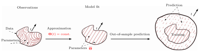
Figure 1. An illustration of a data-driven modelling concept using SDE with constant parameters.

2.2. The Non-Parametric Clustering Methodology

The previous section covers the parameter estimation of a general autonomous SDE, assuming the values of its parameters stay constant in time. If we consider that the data comes from an experiment, then this assumption is more valid for measurements that are carried out in the laboratory under controlled conditions. Contrarily, the experiments with uncontrollable conditions are often hard to reproduce. Consider as an example the atmospheric boundary layer. The duration of a field measurement campaign may extend over several months, providing a time series with a wide range of dynamical regimes (Sun et al.,, 2012; Mahrt,, 2014; Vercauteren et al.,, 2019). It is, therefore, necessary to cluster the data to be able to isolate and understand the associated dynamics. If one decides to model the non-stationary process with an SDE, then the circumstance of time-dependent parameters must be taken into account:

(2.14) $$\textrm{d}X=f(X;\bm{\Theta}(t))\textrm{d}t+g(X;\bm{\Theta}(t))\textrm{d}W_{t}\,$$

(2.15) $$\bm{\Theta}:[0,T]\rightarrow\mathbb{R}^{n}\,,\qquad\bm{\Theta}(t)=[\theta_{1}(t),\theta_{2}(t),\dots,\theta_{n}(t)]\in\Omega_{\bm{\Theta}}$$

To estimate the time-varying parameters, we use the non-parametric clustering approach with smooth regularization introduced by Horenko, 2010a (called FEM-H1) and further developed by Pospisil et al., (2018). Here, the term FEM is used to indicate that the finite dimensional projection space used for the regularization is constructed by mimicking the basic principles of the finite element method. Moreover, ”H1” symbolizes that the finite dimensional projection space is a subspace of $H^{1}(0,T)$. Thereby, the task of identifying $\bm{\Theta}(t)$ via FEM-H1 consists of solving two different inverse problems, which are coupled together into one estimation procedure. The first problem consists of identifying fixed parameter values, and the second problem is identifying their location in time. In the following, we focus on the second task. The FEM is adopted to simplify the task complexity in determining the approximation of the time-variable parameter $\bm{\Theta}(t)$. Since the term FEM is commonly associated with partial differential equations, we note that this is not the purpose here.

The problem of parameter estimation (see Eq. (2.3)) becomes ill-posed, if we try to estimate a set of time-dependent parameters, because we try solve a high-dimentional problem.

To overcome this difficulty, Horenko, 2010a suggests regularizing the fitness function by assuming that the process $X(t)$ varies much faster than the parameter function $\bm{\Theta}(t)$. Formally, this means expressing the fitness function with a convex combination of $K$ locally-optimal fitness functions,

(2.16) $$l_{N}(\bm{\Theta}(t)):=\sum_{i=0}^{N-1}\sum_{k=1}^{K}\gamma_{k}(t_{i})\,f(t_{i};\overline{\bm{\theta}}_{k})\,,\quad K\geq 2\,,$$

where $f(t_{i};\overline{\bm{\theta}}_{k})$ is the time-dependent fitness function formed by the time-averaged parameter value $\overline{\bm{\theta}}_{k}$. The overbar denotes the averaged value, which is assumed to be constant. The value of $K$ indicates the number of clusters or sub-models. The functions $\gamma_{k}(t)$ are the affiliation functions with specific properties explained later. They are unknown and will be estimated with an additional step described later too. The function $f(\cdot;\cdot)$ is taken to be equivalent to the Eq. (2.2) and is defined as

(2.17) $$f(t_{i};\overline{\bm{\theta}}_{k}):=-\textrm{ln}\left[p_{X}(\Delta t,X(t_{i+1})|X(t_{i});\overline{\bm{\theta}}_{k})\right]\,,\qquad i=1,\dots,N-1\,,$$

where the index $i$ iterates over the observations. We keep the sample size of $f(\cdot;\cdot)$ equal to the sample size of $X$ by setting the value at the last timestep $N$ to be equal to the first one $f(t_{N};\overline{\bm{\theta}}_{k})=f(t_{1};\overline{\bm{\theta}}_{k})$. The affiliation functions $\gamma_{k}(t)$ contain information on the location of the minima for each of the $k$-th $f(\cdot;\cdot)$ and are grouped in the so-called affiliation vector $\bm{\Gamma}(t)=[\gamma_{1}(t),\gamma_{2}(t),\dots,\gamma_{K}(t)]\in\mathbb{R}^{K}$. The functions $\gamma_{k}(t)$ satisfy the convexity constrains forming the partition of unity,

(2.18) $$\sum_{k=1}^{K}\gamma_{k}(t) =1\,,\qquad\forall t\,\in[0,T],$$

(2.19) $$1\geq\gamma_{k}(t) \geq 0\,,\qquad\forall t\in[0,T],k\,.\,$$

The vector $\bm{\Gamma}(t)$ represents a vector of time-dependent weights. The functions $\gamma_{k}(t)$ define the activity of an appropriate $k$-th SDE at a given time $t$ (Pospisil et al.,, 2018), or serves as a $K$-dimensional probability vector, which expresses a certainty to observe the $k$-th stationary model at time $t$. For example, assuming that we know the affiliation vector in advance the temporal evolution of one parameter function is:

(2.20) $$\theta(t)=\sum_{k=1}^{K}\gamma_{k}(t)\overline{\theta}_{k}+\varepsilon(t)\,,$$

where $\theta(t)$ is approximated by $K>2$ piecewise constant values $\overline{\theta}$ (see Fig. 2) and $\varepsilon(t)$ is some approximation error.

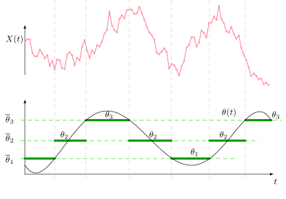
Figure 2. Sketch explaining the approximation for one of the time-dependent parameter functions with piecewise constant subdivisions.

As an example, Figure 2 illustrates the approximation of one non-stationary parameter with $K=3$. The figure indicates a variable location and period of each subdivision which depends on the evolution of $\theta(t)$ and the number of clusters used. This information is encoded in the $\bm{\Gamma}(t)$ function. For $K\rightarrow N$ the approximation of $\theta(t)$ gets better. With each additional cluster used, a different additional set of parameters need to be determined. If the number of clusters equals the number of points in the time series ($K=N$), each point should be potentially described by one equation with its unique parameter values. If, for example, an equation with $3$ parameters is considered, the time series of length $N$ is modeled using $3N$ parameters. Such an approximation is considered to be overfitting. An additional consequence is that the uncertainty for each estimate of $\overline{\theta}_{k}$ grows (see Eq. (2.4)) because the amount of data available for each cluster reduces (i.e. each SDE model).

The averaged clustering functional $L_{N}$ together with the assumptions (2.16), (2.18), (2.19) and the fitness function (Eq. (2.17)) becomes:

(2.21) $$L_{N}(\bm{\Gamma}(t),\overline{\bm{\theta}}_{1},\dots,\overline{\bm{\theta}}_{K})=-\sum_{i=0}^{N-1}\sum_{k=1}^{K}\gamma_{k}(t_{i})\,\textrm{ln}\left[p_{X}(\Delta t,X(t_{i+1})|X(t_{i});\overline{\bm{\theta}}_{k})\right]\,.$$

Applying the regularization and the discretization with the finite element method the functional becomes:

(2.22) $$L^{\epsilon}_{\widehat{N}}(\bm{\Gamma}(\tau),\overline{\bm{\Theta}},\epsilon^{2})=\sum_{k=1}^{K}\left[b(\tau,\overline{\bm{\theta}}_{k})^{\top}\gamma_{k}(\tau)+\epsilon^{2}\gamma_{k}(\tau)^{\top}\bm{A}\gamma_{k}(\tau)\right]\rightarrow\underset{\bm{\Gamma}(\tau),\overline{\bm{\Theta}}}{\textrm{min}}\,.$$

where the vector $\bm{\Gamma}(\tau)=[\gamma_{1}(\tau),\gamma_{2}(\tau),\dots,\gamma_{K}(\tau)]\in\mathbb{R}^{K\times\widehat{N}}$ is the coarsened version of $\bm{\Gamma}(t)$. Here, $\tau$ denotes the reduced $t$ grid by a factor $\alpha\in(0,1]$ and distinguish the notation of the vector $\bm{\Gamma}(t)$ from $\bm{\Gamma}(\tau)$. For additional details on the FEM approximation of $\gamma_{k}(\tau)$ and the construction of $\bm{A}$ see Horenko, 2010a and Metzner et al., (2012)).

The coarser and uniform mesh with its size $\Delta\tau$ is a set of points $(\tau_{j})_{0\leq j\leq\widehat{N}+1}$ with the respective intervals $\mathcal{T}_{j}=[\tau_{j},\tau_{j+1}]$ where $0=\tau_{0}<\tau_{1}<\dots<\tau_{\widehat{N}+1}=T$ such that the new number of discretization points $\widehat{N}<N$ .

The Lagrange $\mathbb{P}_{1}$ elements associate with the space of globally continuous, locally linear functions for every interval $\Delta\tau$:

(2.23) $$V_{\Delta\tau}=\{v_{\Delta\tau}\in C^{0}([0,T]):v_{\Delta\tau}|\mathcal{T}_{j}\in\mathbb{P}_{1},0\leq j\leq\widehat{N}\}\,,$$

with the subspace:

(2.24) $$V_{0,\Delta\tau}=\{v_{\Delta\tau}\in V_{\Delta\tau}:v_{\Delta\tau}(0)=v_{\Delta\tau}(T)=0\}\,.$$

The first term $b(\cdot,\cdot)^{\top}\gamma_{k}(\cdot)$ in Eq. (2.22) is the discretized version of $L_{N}(\cdot,\cdot)$ (see Eq. (2.21)) and is formulated as a dot product. The symbol $\top$ indicates the transpose of the corresponding vector. The vector $b(\tau,\overline{\bm{\theta}}_{k})$ denotes the discretized model fitness function,

(2.25) $$b(\tau,\overline{\bm{\theta}}_{k})=\left(\int_{\tau_{1}}^{\tau_{2}}f(t,\overline{\bm{\theta}}_{k})v_{1}(t)\textrm{d}\tau,\dots,\int_{\tau_{\widehat{N}-1}}^{\tau_{\widehat{N}}}f(t,\overline{\bm{\theta}}_{k})v_{\widehat{N}}(t)\textrm{d}\tau\right)\,,$$

where $v(t)$ is the hat function and $f(\cdot,\cdot)$ the function in Eq. (2.17). The operation in Eq. (2.25) is denoted as the reduction and it projects a vector into the space of the finite element. Consequently, the function $f(\cdot,\cdot)$ changes its sampling rate from $\Delta t$ to a larger mesh size $\Delta\tau$. The second term $\epsilon^{2}\gamma_{k}(\tau)^{\top}\bm{A}\gamma_{k}(\tau)$ penalizes the functional by controlling the regularity of the vector $\bm{\Gamma}(\tau)$, which is required to obtain a valid solution. With the $\mathbb{P}_{1}$ elements , the cluster respective stiffness matrix $\bm{H}_{k}$ assembles to

$$\bm{H}_{k}=\begin{pmatrix}2&-1&0&\cdots&0\\ -1&2&-1&\cdots&0\\ 0&-1&2&\cdots&0\\ \vdots&\vdots&\vdots&\ddots&\vdots\\ 0&0&0&\cdots&2\end{pmatrix}\in\mathbb{R}^{\widehat{N}\times\widehat{N}}\,,\quad k=1,\dots,K\,.$$

and the total stiffness matrix

$$\bm{A}=\begin{pmatrix}\bm{H}_{1}&0&\cdots&0\\ 0&\bm{H}_{2}&\cdots&0\\ \vdots&\vdots&\ddots&\vdots\\ 0&0&\cdots&\bm{H}_{K}\end{pmatrix}\in\mathbb{R}^{K\widehat{N}\times K\widehat{N}}\,.$$

The regularized variational problem Eq. (2.22) is solved iteratively:

1. Fix $\bm{\Gamma}(t)$ and find $\overline{\bm{\Theta}}^{\ast}$ by solving $L_{N}(\bm{\Gamma}(t),\overline{\bm{\Theta}})\rightarrow\underset{\overline{\bm{\Theta}}}{\textrm{min}}$ (2.21)

2. Fix $\overline{\bm{\Theta}}$ and find $\bm{\Gamma}^{\ast}(\tau)$ by solving $L^{\epsilon}_{\widehat{N}}(\bm{\Gamma}(\tau),\overline{\bm{\Theta}},\epsilon^{2})\rightarrow\underset{\bm{\Gamma}(\tau)}{\textrm{min}}$ (2.22)

The second step is a problem with a quadratic cost function formed by linear equality and inequality constrains, which is reformulated from Eq. (2.22) by defining column vectors from $K$ clusters. The so-called vector of modeling errors $\bm{B}(\tau)$ (Pospisil et al.,, 2018) is constructed using the reduced local fitness function Eq. (2.25),

(2.26) $$\bm{B}(\tau):=[b(\tau,\overline{\bm{\theta}}_{1}),b(\tau,\overline{\bm{\theta}}_{2}),\ldots,b(\tau,\overline{\bm{\theta}}_{K})]\in\mathbb{R}^{K\widehat{N}}\,,$$

From Eq. (2.22) the block-structured quadratic programming (QP) problem is:

(2.27) $$\bm{\Gamma}^{\ast}(\tau) :=\textrm{arg }\underset{\bm{\Gamma}\in\Omega_{\Gamma}}{\textrm{min }}L^{\epsilon}_{\widehat{N}}(\bm{\Gamma}(\tau),\overline{\bm{\Theta}},\epsilon^{2})\,,$$

(2.28) $$L^{\epsilon}_{\widehat{N}} :=\frac{1}{\widehat{N}}\bm{B}^{\top}(\tau)\bm{\Gamma}(\tau)+\frac{1}{\widehat{N}}\epsilon^{2}\bm{\Gamma}^{\top}(\tau)\bm{A}\bm{\Gamma}(\tau)\,,$$

(2.29) $$\Omega_{\Gamma} :=\{\bm{\Gamma}(\tau)\in\mathbb{R}^{K\widehat{N}}:\bm{\Gamma}(\tau)\geq 0\,\wedge\,\sum_{k=1}^{K}\gamma_{k}(\tau)=\bm{1}\,\forall t\in[0,T]\}\,,$$

where $1/\widehat{N}$ is a scaling coefficient to avoid large numerical values. To solve the QP, we use the adapted spectral projected gradient method developed by Pospisil et al., (2018). Their method enjoys high granularity of parallelization and is suitable to run on GPU clusters. Furthermore, it is efficient and outperforms traditional denoising algorithms in terms of the signal-to-noise ratio.

Reducing the samples size to $\widehat{N}<N$ reduces the size of the QP problem, and its computational complexity. Higher-order elements also require additional collocation points, but offer smoother approximations. However, the accuracy in determining $\overline{\bm{\Theta}}^{\ast}$ depends on the number of available observations as it scales with $1/\sqrt{N}$ and needs, therefore, to be solved at the smallest available time step $\Delta t$. If we now reduce the size of the QP problem (see Eq. (2.25)) the accuracy of the estimate $\overline{\bm{\Theta}}^{\ast}$ will decrease. Consequently, we cannot solve both problems at the same timestep $\Delta\tau$ and need to interpolate the solution of QP in each iteration step. This is done as follows:

1. Fix $\bm{\Gamma}(t)$ and find $\overline{\bm{\Theta}}^{\ast}$ by solving $L_{N}(\bm{\Gamma}(t),\overline{\bm{\Theta}})\rightarrow\underset{\overline{\bm{\Theta}}}{\textrm{min}}$

2. reduce the fitness function to the $\tau$-grid

3. Fix $\overline{\bm{\Theta}}$ and find $\bm{\Gamma}^{\ast}(\tau)$ by solving $L^{\epsilon}_{\widehat{N}}(\bm{\Gamma}(\tau),\overline{\bm{\Theta}},\epsilon^{2})\rightarrow\underset{\bm{\Gamma}(\tau)}{\textrm{min}}$

4. interpolate $\bm{\Gamma}^{\ast}(\tau)$ to the $t$-grid step size $\Delta t$

1

2

Input : Time series $X$, number of clusters $K$, regularisation value $\epsilon^{2}$ and the reduction value $\alpha$

Output : $\bm{\Gamma}^{\ast}(t)$ and $\overline{\bm{\Theta}}^{\ast}$

3

4Generate random initial $\bm{\Gamma}^{0}(t)$ satisfying 2.18 and 2.19

5/* We need the full $\bm{\Gamma}^{0}(t)$ to find $\overline{\bm{\Theta}}$ and the reduced $\bm{\Gamma}^{0}(\tau)$ to solve the QP problem */

6

7Reduce the initial vector $\bm{\Gamma}^{0}(t)$ to $\bm{\Gamma}^{0}(\tau)$ on the coarser grid $\Delta\tau$

8Set iteration counter $j=0$ for the main optimization loop

9/* main optimization loop */

10 while $\left|L^{\epsilon}_{\widehat{N}}(\bm{\Gamma}^{j+1}(\tau),\overline{\bm{\Theta}}^{j+1},\epsilon^{2})-L^{\epsilon}_{N}(\bm{\Gamma}^{j}(\tau),\overline{\bm{\Theta}}^{j},\epsilon^{2})\right|$ $>$ tol do

11      

12      /* Estimate $\overline{\bm{\Theta}}^{j}$ from the full (This will ensure maximum accuracy for the estimate of $\overline{\bm{\Theta}}^{j}$) $\bm{\Gamma}^{j}(t)$ applying $K$ times unconstrained minimization */

13       for $k\leftarrow 1$ to $K$ do

14             $\overline{\bm{\theta}}_{k}^{j+1}=\underset{\bm{\theta}}{\textrm{arg min}}\,L_{N}(\gamma_{k}^{j}(t),\bm{\theta})$ // See eq. 2.21.

15       end for

16      /* From the found $\overline{\bm{\theta}}_{k}^{j+1}$ compute the fitness functions $f^{j+1}(t,\overline{\bm{\theta}}_{k}^{j+1})$ or save it from the step in line 9 */

17      

18      Compute $f^{j+1}(t,\overline{\bm{\theta}}_{k}^{j+1})$, if not saved from line 9 //

19      /* Reduce $f^{j+1}(t,\overline{\bm{\theta}}_{k}^{j+1})$ because $\bm{\Gamma}(\tau)$ will be estimated on the coarser grid $\Delta\tau$ */

20      

21      Compute $b^{j+1}(\tau,\overline{\bm{\theta}}_{k}^{j+1})=reduction(f^{j+1}(t,\overline{\bm{\theta}}_{k}^{j+1}),\Delta\tau,\alpha)$ // See eq. 2.25

22      /* Apply quadratic programming to solve the constrained minimization */

23      

24      $\bm{\Gamma}^{j+1}(\tau)=\underset{\bm{\Gamma}}{\textrm{arg min}}\,L^{\epsilon}_{\widehat{N}}(\bm{\Gamma}(\tau),b^{j+1}(\tau,\overline{\bm{\theta}}_{k}^{j+1}),\epsilon^{2})$  satisfying 2.18 and 2.19

25      /* Interpolate $\bm{\Gamma}^{j+1}(\tau)$ onto the original grid with a scale $\Delta t$ */

26      

27      $\bm{\Gamma}^{j+1}(t)=interpolate(\bm{\Gamma}^{j+1}(\tau),\Delta t)$

28      /* Addvance the main loop counter j */

29      

30      $j=j+1$

31 end while

32

return $\bm{\Gamma}^{j+1}(t)$, $\overline{\bm{\Theta}}^{j+1}$

Algorithm 1 The adapted subspace algorithm for SDE models. The main change to the original version of he algorithm is in line 9, where the functional $L_{N}$ is formulated for a general SDE. Furthermore, lines 14 and 18 are added to maintain the accuracy of the estimated $\overline{\bm{\Theta}}^{\ast}$. The reduced variables are indicated by the time variable $\tau$ and the non-reduced with $t$, respectively. See Appendix A for more details.

In that way, we keep the stepsize of the $\bm{\Theta}$ solver step (1) ($\Delta t$) separated from the stepsize of the $\bm{\Gamma}$ solver (3) ($\Delta\tau$ ), ensuring an accurate approximation of $\overline{\bm{\Theta}}$ while keeping the benefit of the FEM. The algorithm 1 to solve the variational problem (2.22) is called the subspace clustering algorithm (Horenko, 2010a, ) and is reproduced with the proposed modification.

After a successful application of the clustering method, one has several directions for further research. For instance, the vector $\bm{\Gamma}^{\ast}(t)$ provides a classifier and can be used to analyze quantities of interest across the clusters. Instead, we demonstrate a way how the vector $\bm{\Gamma}^{\ast}(t)$ can be used to construct stochastic closures to effectively model unresolved degrees of freedom as modulated by resolved variables behaviour.

2.3. Stochastic Closure

One difficulty in finding a stochastic closure is the missing information regarding the future realization of the vector $\bm{\Gamma}^{\ast}(t)$ because it is an estimate that is based on the available data. Although we have assumed that we observe a sufficient amount of data to capture the full range of regime dynamics, we are incapable of predicting the future state of the vector $\bm{\Gamma}(t)$ without additional assumptions and modeling work. One can associate the affiliation function with a Markov process, assuming that it is homogeneous and stationary (Metzner et al.,, 2012). Alternatively, Kaiser et al., (2017) applied a neural network within the clustering framework to predict the velocity components of internal gravity waves beyond the training data set.

We show a different approach by regressing the clustered parameter values to some known auxiliary process $u(t)$. The limitation is then that it may not always be possible to find such a process. However, in the case of existence, no assumptions are required. This approach is attractive since the process $u(t)$ should exist on a larger scale than the process $X(t)$ and thus be predictable.

For simplicity, suppose we are presented with an observation of a slowly evolving, known process $u(t)$ and a fast non-stationary, stochastic process $X(t)$ described by some nonlinear SDE. Furthermore, suppose that we have access to some expert knowledge, intuition or first principle derivation suggesting that $u(t)$ is controlling the non-stationary process $X(t)$ by modulating its model parameters. The closure approach is then the following. First one estimates the time-varying parameters of the SDE:

(2.30) $$\textrm{d}X=f(X;\bm{\Theta}(t))\textrm{d}t+g(X;\bm{\Theta}(t))\textrm{d}W_{t}\,$$

(2.31) $$\bm{\Theta}:[0,T]\rightarrow\mathbb{R}^{n}\,,\qquad\bm{\Theta}(t)=[\theta_{1}(t),\theta_{2}(t),\dots,\theta_{n}(t)]\in\Omega_{\bm{\Theta}},$$

with the clustering approach presented in section 2.2 that is by solving the variational problem:

(2.32) $$(\bm{\Gamma}^{\ast},\overline{\bm{\Theta}}^{\ast})\in\underset{\bm{\Gamma}\in\Omega_{\bm{\Gamma}}}{\underset{\bm{\Theta}\in\Omega_{\bm{\Theta}}}{\textrm{arg min}}}\,\,L^{\epsilon}_{\widehat{N}}(\bm{\Gamma},\overline{\bm{\Theta}},\epsilon^{2})\,,$$

where the number of clusters $K\geq 2$. The functional $L_{\widehat{N}}^{\epsilon}$ is defined in Eq. (2.22).

Second, with the help of $\bm{\Gamma}^{\ast}(t)$ one estimates the cluster respective values of the process $u(t)$ by computing the weighted average:

(2.33) $$\overline{u}_{k}=\frac{\sum_{i=1}^{N}u(t_{i})\gamma_{k}(t_{i})}{\sum_{i=1}^{N}\gamma_{k}(t_{i})}\,,\qquad k=1,\dots,K\,.$$

where $\overline{u}_{k}$ denotes the averaged value of the auxiliary process $u(t)$ in cluster $k$. Recall that the $\gamma_{k}(t_{i})$ is the affiliation function for cluster $k$ (see Fig. 8a the color coded regions). In the last step, one performs a regression analysis to parameterize the parameter variability with some appropriate functions $S_{m}$, which map the values of $u(t)$ to $\theta_{m}(t)$:

(2.34) $$S_{m}:\overline{u}_{k}\rightarrow\overline{\bm{\theta}}_{k,m}\,,\qquad\overline{\bm{\theta}}_{k}=[\overline{\theta}_{k,1},\overline{\theta}_{k,2},\dots,\overline{\theta}_{k,n}],\qquad k=1,\dots,K\,\qquad\,m=1,\dots,n.$$

There is no restriction on the differentiability of the functions $S_{n}$, it can be parameterized by a piecewise-defined function. The parameterization is performed for each element of the parameter vector $\bm{\Theta}$ separately. The vector of scaling functions $\bm{S}=[S_{1},S_{2},\dots,S_{n}]\in\mathbb{R}^{n}$ defines the modulation of the model parameters through some process $u(t)$. The complexity of the relation is application dependent and needs further exploration. If all scaling functions can be found, we obtained a closed system to predict the process $X(t)$

(2.35) $$\textrm{d}X=f(X;\bm{S}(u(t)))\textrm{d}t+g(X;\bm{S}(u(t)))\textrm{d}W_{t}\,,$$

where $u(t)$ is known for every $t$. The approach allows to model non-equilibrium processes which are characterized by the nonlinearity in $f$ and $g$ in the cases where the nonstationarity of the process is difficult to understand. Figure 3 summarizes the idea of this concept. In practice the functional relation between process $u(t)$ and the modulated parameters of the SDE $\bm{\Theta}(t)$ is assumed to hold for the estimated parameter range, as shown in Section 5.

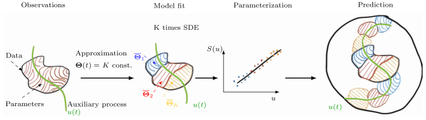
Figure 3. The modeling approach with FEM-H1 regularization of SDE. The temporal modulation of the parameters is parameterized through the slow scale process $u$. The functional relation $S(u)$ is hidden and needs to be discovered a posteriori.

3. Selection of the Hyperparameters

The selection of a suitable model includes the determination of a suitable regularization parameter $\epsilon^{2}$ , controlling the smoothness of the affiliation vector, the number of clusters $K$ and the functional forms $f(\cdot;\cdot)$ and $g(\cdot;\cdot)$. A variety of strategies with examples are described in (Horenko, 2010a, ; Horenko, 2010b, ; Metzner et al.,, 2012) for example, which are partially based on identifying several criteria simultaneously. Here we present new approaches to select $\epsilon^{2}$ and $K$ independently from each other, providing a robust estimation strategy. In particular our approach for selecting the parameter $\epsilon^{2}$ accounts indirectly for the frequency content of the auxiliary process $u(t)$.

3.1. Optimal Regularization Parameter

Horenko, 2010a analyzed the impact of the parameter $\epsilon^{2}$ on the regularity of the cluster affiliation function $\bm{\Gamma}^{\ast}(t)$. His findings show that the optimal parameter $\epsilon^{2}_{\text{opt}}$ is characterized by a sharp separation between each of the functions $\gamma_{k}(t)$, such that the regime transitions are as short as possible. Contrary, poor partitioning is present if two or more functions $\gamma_{k}(t)$ occupy the same period. We recall, that the functions $\gamma_{k}(t)$ obey the convexity condition (see Eq. (2.18); (2.18)) and if several are active simultaneously then none of the model parameters fits the data sufficiently well. Such results indicate that the number of clusters is set too high or the model structure is not suitable for the data under consideration. A key aspect of choosing a proper value for $\epsilon^{2}$ is in monitoring the regularity of the affiliation function $\bm{\Gamma}^{\ast}(t)$. Figure 4 shows a portion of $\bm{\Gamma}^{\ast}(t)$ with $K=3$ for a toy example.

To motivate the strategy in finding $\epsilon^{2}_{opt}$ we consider $\bm{\Gamma}^{\ast}(t)$ for different values of the parameter (see Fig. 4a, b, c). Note the white regions between $0$ and $1$ in Fig. which are not color coded. The total size of this area is changing in each of the panels and is approximately the smallest at the value of $\epsilon^{2}_{opt}$. If we consider the function $\bm{\Gamma}^{\ast}(t)$ as an oscillating signal, then to minimize the white area we search for a $\bm{\Gamma}^{\ast}(t)$ that has the largest energy, where energy is understood as $||\gamma_{k}||^{2}_{L^{2}(0,T)}$. Using the cluster averaged signal energy $E_{\gamma}$ for a given value $\epsilon^{2}$

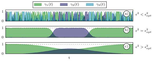
Figure 4. An example on the different regularity of the affiliation vector $\bm{\Gamma}^{\ast}(t)$. Each panel displays the same time window but for different values of $\epsilon^{2}$. a) The weak regularization: the regime periods are irregular. Their temporal scale is close to $\textrm{d}t$. b) The optimal regularization: $\gamma_{1}(t)$ and $\gamma_{2}(t)$ shows relatively sharp and clear separation. c)The strong regularization: $\gamma_{2}(t)$ is blurred and suppressed.

(3.1) $$E_{\gamma}(\epsilon^{2})=\frac{1}{K}\sum_{k=1}^{K}\int_{0}^{T}\gamma_{k}^{2}(t,\epsilon^{2})\textrm{d}t\,,$$

where $\gamma_{k}^{2}(t,\epsilon^{2})$ is the solution of Eq. (2.22), we determine the value $\epsilon^{2}$ that maximize the energy. The maximum of the curve $E_{\gamma}(\epsilon^{2})$ indicates the optimal regularization value (see Fig. 5 color code value $0$). The true affiliation function which was used to generate the training data is generated with sharp transitions and three clusters. Furthermore, in the identification step, we used the same functional form that was used in the construction process. In other words, the considered examples are well-posed in the sense that the data-generating model is perfectly identifiable. However, working with real, unexplored data we, unfortunately, may not know the true functional form of the SDE. This may lead to a situation where the functions $\gamma_{k}(t)$ are uncertain which affects the curve $E_{\gamma}(\epsilon^{2})$ by making it less concave and hence loosing a pronounced maximum. This is an indication of an increased sensitivity. To achieve a more robust procedure we investigate the frequency content of the vector $\bm{\Gamma}^{\ast}(t)$.

One way to emphasize the maximum of the curve $E_{\gamma}(\epsilon^{2})$ is by gradually removing the high frequency oscillations in $\bm{\Gamma}^{\ast}(t)$. Since the affiliation function is not periodic we filter it with a wavelet method (Foufoula-Georgiou and Kumar,, 1994). The affiliation vector is decomposed using the discrete wavelet transform to obtain $C$ levels with $C+1$ frequency bands. The function $\gamma_{k}(t)$ is then represented as the sum of the low-frequency component $\gamma_{k,C}^{A}(t)$ after $C$ levels of transformations and the sum of the high-frequency components $\gamma_{k,c}^{D}(t)$ over the previous decomposition levels

(3.2) $$\gamma_{k}(t)=\gamma_{k,C}^{A}(t)+\sum_{c=1}^{C}\gamma_{k,c}^{D}(t)\,.$$

As a basis for the filtering, we choose the Haar wavelet. They represent the sharp jumps of the affiliation vector in the best way, especially when approaching the value $\epsilon^{2}_{opt}$. Utilizing the $L_{2}$-orthogonality property of the Haar wavelets one inserts Eq. (3.2) in to (3.1) to obtain

(3.3) $$E_{\gamma}(\epsilon^{2})=\frac{1}{K}\sum_{k=1}^{K}\int_{0}^{T}\left[\gamma_{k,C}^{A}(t)\right]^{2}\textrm{d}t+\frac{1}{K}\sum_{k=1}^{K}\int_{0}^{T}\left[\sum_{c=1}^{C}\gamma_{k,c}^{D}(t)\right]^{2}\textrm{d}t\,.$$

The signal $\gamma_{k}(t)$ is decomposed with the maximum number of possible levels $C$, which is dependent on the number of samples. The first term in Eq. (3.3) is the mean value of the total time series and is irrelevant since we are interested in regime transitions between different models. In the following steps we keep the same notation for $E_{\gamma}(\epsilon^{2})$. The local-support property of the wavelets allows to take out the summation sign of the integral,

(3.4) $$E_{\gamma}(\epsilon^{2})=\frac{1}{K}\sum_{k=1}^{K}\sum_{c=1}^{C}\int_{-\infty}^{\infty}\left[\gamma_{k,c}^{D}(t)\right]^{2}\textrm{d}t\,.$$

The sample size of the discrete-time series $\gamma_{k,c}^{D}(t)$ is extended to the nearest value $2^{i}$ with the reflect-padding method, where $i\in\mathbb{N^{+}}$. Next, we rewrite the continuous integral as a sum

(3.5) $$E_{\gamma}(\epsilon^{2})=\frac{1}{K}\sum_{k=1}^{K}\sum_{c=1}^{C}\sum_{d=1}^{C_{d}}\left[\tilde{\gamma}_{k,c}^{D}(d)\right]^{2}\Delta t\,,$$

where $C_{d}(c)$ denotes the number of coefficients at the decomposition level $c$. Due to the efficient implementation of the multi-resolution decomposition the number of coefficients at each level is consecutively reduced by $2$. With each decomposition level the cut-off frequency is halved and the energy of the resulting frequency bands can be removed by setting the corresponding coefficients to zero.

The optimal cut-off frequency may be estimated in several ways. A reasonable choice would be to set it to the scale of a spectral gap, if one is present, between the process $X(t)$ and $u(t)$. A spectral gap is formed when the highest frequency of $u(t)$ is larger than the lowest frequency of $X(t)$. In this way, the scale of the process $u(t)$ provides a limit for the smallest scale of the regime jumps in $\bm{\Theta}(t)$. There is no need to define the upper bound because the curve $E_{\gamma}(\epsilon^{2})$ drops naturally due to the over-smoothing of the vector $\gamma_{k}(t)$ at higher values $\epsilon^{2}$. The over-smoothing is not detected by the sharp jumps of the Haar wavelet basis. Consequently, the wavelets stop registering the energy at the respective scales (see the roll-off in Fig. 5 for $\epsilon^{2}>10^{2}$). Alternatively, one plots the energy curves by consecutively removing the high frequencies and looks for a magnification of a maximum without a change in its position (see Fig. 5). The multi-resolution analysis is performed using the python library PyWavelets (Lee et al.,, 2019).

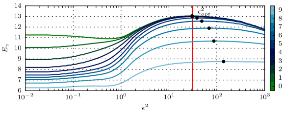
Figure 5. An approximation of the optimal regularisation parameter $\epsilon^{2}$ for a toy example with three clusters. The y-axis is the cluster averaged signal energy of $\bm{\Gamma^{\ast}}(t)$ (see Eq. 3.5). By wavelet filtering the estimated affiliation vector we emphasize the maximum. The colorbar labels the number of removed details coefficients levels ($9$ of maximum $16$ is shown). The zero marks the unfiltered $\bm{\Gamma^{\ast}}(t)$. In this example one can exclude four levels to emphasise the maximum without compromising the optimum.

3.2. Optimal Number of Clusters K

The approach to determine the optimal number of clusters $K_{\text{opt}}$ is borrowing ideas from the elbow method which is used in the K-means clustering approach (Yuan and Yang,, 2019). The idea is to monitor an error measure for the clustering procedure over the number of clusters and search for a characteristic ”kink” in the graph. The choice of the error measure is, therefore, important and specific to the method used. For instance, a measure of compactness in K-means clustering is defined as the sum of the Euclidean intra-cluster distances between points in a given cluster. We introduce a different error measure because the SDE clustering method differentiates the temporal dynamics within the clusters. Two clusters may strongly overlap but be distinct in terms of their induced stationary probability density functions. The Euclidean distance would be a poor choice in that case. Instead, we exploit the Kullback-Leibler (KL) divergence, which is closely related to the probability density of the SDE:

(3.6) $$KL(P||Q):=\int P(x)\,\textrm{log}\left(\frac{P(x)}{Q(x)}\right)\textrm{d}x\,.$$

The KL divergence describes the information gain by changing from the distribution with density $P$ to the distribution with density $Q$. Here we will use the $P$ and $Q$ as the stationary distributions of two different clusters. We seek to measure the difference between $P$ and $Q$ or more generally the diversity between $K$ stationary distributions. Due to the asymmetry of KL divergence we consider also the values of the opposite divergences $KL(Q||P)$. Let $p^{\star}_{k}$ denote the stationary distribution of an SDE with the estimated parameter set $\overline{\bm{\theta}}^{\ast}_{k}$ and the corresponding $\gamma_{k}(t)$ for cluster $k=1,\dots,K$. For each cluster we thus have a different SDE model that provides a stationary distribution. We define the weighted diversity matrix $D=(d_{ij})\in\mathbb{R}^{K\times K}$ computed as

(3.7) $$d_{ij}:=KL(p_{i}^{\star}||p_{j}^{\star})=\nu_{j}\int p_{i}^{\star}\,\textrm{log}\left(\frac{p_{i}^{\star}}{p_{j}^{\star}}\right)\textrm{d}x\,\geq 0\qquad i,j=1,\ldots\,K\,,$$

where $\nu_{j}$ are the weights computed from the affiliation vector that quantify the relative frequency of cluster $j$:

(3.8) $$\nu_{j}=\int_{0}^{T}\gamma_{j}(t)\textrm{d}t\,,\qquad j=1,\ldots K\,.$$

The weights are introduced for the following reason. By adding more clusters the less probable ${\gamma_{j}}(t)$ is suppressed (see for example Fig. 4c) and barely reaches values equal to $1$ or it has a short lifetime relative to the full-time horizon $T$. These suppressed, less-probable, inactive regimes should therefore include less diversity and compensate the measure. Since we are looking to find the optimal number of cluster within some reasonable range $2<K<K_{\text{max}}$ we define our diversity measure of clustering with $K$ clusters as:

(3.9) $$W_{K}=\sum_{i=1}^{K}\sum_{j=1}^{K}d_{ij}\,,\qquad K=2,3,\ldots,K_{\textrm{max}}\,,$$

where $K_{\textrm{max}}$ denotes the maximum considered clusters, assuming that $2<K_{\textrm{opt}}<K_{\textrm{max}}$. We reiterate that $p^{\star}_{k}$ in Eq. (3.7) denotes the stationary distribution of the SDE model characterized by parameter set $\overline{\bm{\theta}}^{\ast}_{k}$. Specifically, for the SDE model

(3.10) $$\textrm{d}X=f(X;\overline{\bm{\theta}}^{\ast}_{k}))\textrm{d}t+g(X;\overline{\bm{\theta}}^{\ast}_{k}))\textrm{d}W_{t}\,,\qquad k=1,\dots,K\,,$$

the invariant density $p^{\star}_{k}$ can be written as

(3.11) $$p^{\star}_{k}(X)=\frac{N_{c}}{g^{2}(X;\overline{\bm{\theta}}^{\ast}_{k})}\textrm{exp}\left(\int\frac{2f(X;\overline{\bm{\theta}}^{\ast}_{k})}{g^{2}(X;\overline{\bm{\theta}}^{\ast}_{k})}dx\right)\,,\qquad k=1,\ldots K\,,$$

where the normalisation constant $N_{c}$ is:

(3.12) $$N_{c}^{-1}=\int\frac{1}{g^{2}(X;\overline{\bm{\theta}}^{\ast}_{k})}\textrm{exp}\left(\int\frac{2f(X;\overline{\bm{\theta}}^{\ast}_{k})}{g^{2}(X;\overline{\bm{\theta}}^{\ast}_{k})}dx\right)\,,\qquad k=1,\ldots K\,,$$

provided all terms are well-defined (see Horsthemke, (1984)[ch. 6.1] for details).

In real-world applications the gain in the diversity $W_{K}$ can be too steady making the detection of $K_{\textrm{opt}}$ difficult. We use further extension of the elbow method idea to make the estimation of $K_{\textrm{opt}}$ robust. Indeed, we follow Tibshirani et al., (2001) where it has been suggested to measure the increase of $W_{K}$ with respect to some null reference distribution. Namely, a data set which has no obvious clustering. In the work of Tibshirani et al., (2001) the randomly spreading of points in 2-dimensional space serves as a null reference data set, which is suitable for clustering with the K-means method. By considering the properties of our clustering method we choose the Wiener process with reflecting boundaries as the null reference time series. The optimal number of clusters is estimated as the point where we get the smallest distance between the clustering-diversity measure of the analyzed and the reference data:

(3.13) $$\textrm{Gap}(K)=\mathbb{E}[\textrm{log}(W_{K}^{\ast})]-\textrm{log}(W_{K})\,,$$

where $W_{K}^{\ast}$ denotes the diversity measure of the null reference dataset and the extracted value $\mathbb{E}[\textrm{log}(W_{k}^{\ast})]$ is estimated from clustering $B\gg 1$ different, independent reference time series. The boundaries for the reference Wiener process is confined to the range of the analyzed process. The section 5 demonstrates the application of presented approach on controlled numerical examples.

4. Implementation

We have developed our version of the algorithm 1 in the programming language C++. The core components of the FEM-H1 framework, namely: the spectral projected gradient method for the quadratic programming, the FEM reduction and interpolation procedures, and the procedure to generate an initial $\bm{\Gamma}(t)$ are reimplemented from the MATLAB code that is created by original authors Pospisil et al., (2018). For the solution of the $\bm{\Theta}$ problem (see algorithm 1 line 9) we use the NLopt nonlinear-optimization package (G. Johnson,, 2021). It is an interface of many global and local optimization algorithms which can be tested just by changing one parameter. Specifically, we applied a combination of Controlled Random Search (CRS) with local mutation (Price,, 1977, 1983; Kaelo and Ali,, 2006) and the ”PRAXIS” gradient-free local optimization via the ”principal-axis method” (Richard P,, 2013). Our code is GPU accelerated using the CUDA libraries cuSPARSE, Thrust and requires the CUDA version 10.2. The transition density is computed with the MATLAB symbolical toolbox and exported to a C++ code. The template library Thrust made it possible to include the machine-generated code of the transition density $p_{X}$ into the main program flow.

5. Numerical examples

The numerical study consists of three examples with varying complexity. The auxiliary process $u(t)$ here is stochastic with a smooth sample path and a reasonable scale separation between $u(t)$ and $X(t)$. However, in real-world applications the process $u(t)$ represents some characteristic quantity of a dynamical system, with the assumption to control the time-varying parameters of the process $X(t)$.

The numerical examples consist of the step by step construction of a synthetic time series $X(t)$ and the identification of the underlying functional relationship between the parameters of a predefined SDE and some random process $u(t)$. Here it is assumed that the process $u(t)$ is known at any instance of time and it serves as a predictor for the time-varying parameter vector $\bm{\Theta}(t)$. To create the synthetic data set $X(t)$, the process $u(t)$ is used together with the arbitrary created functions $S_{n}(u)$ to generate the evolution of the parameter vector $\bm{\Theta}(t)=[S_{1}(u(t)),S_{2}(u(t)),\dots,S_{n}(u(t))]$. The sample path $X(t)$ is simulated numerically with the predefined SDE, where the parameters are given by $\bm{\Theta}(t)$. The time series $X(t)$ forms the data set of the numerical tests, from which we recover the functions $S_{n}(u)$ and compare them to the one that have been used in the creation step.

5.1. The Underlying Auxiliary Process Model

As a way of defining an auxiliary process that respects the required scale separation between $X(t)$ and $\bm{\Theta}(t)$, we provide a brief explanation of a stochastic dynamical system to simulate a slow-evolving underlying process. A realization of the auxiliary process $u(t)$ is constructed for all examples following the same principle. We utilize the 4-dimensional Ornstein - Uhlenbeck process (OU) supplementing it with the coefficients of the normalized Butterworth polynomials,

(5.1) $$\textrm{d}\bm{U}=-\frac{1}{T_{c}}\bm{A}_{D}\bm{U}\textrm{d}t+\bm{B}\textrm{d}\bm{W}\,,\qquad\bm{U}=[u(t),u_{1}(t),u_{2}(t),u_{3}(t)]\,,$$

where $T_{c}>0$ controls the cut off frequency, $\bm{B}>0$ is the diffusion coefficient. The auxiliary process $u(t)$ is then the first component of the vector $\bm{U}(t)$ The diffusion matrix $\bm{B}$ is almost everywhere zero, and together with the drift matrix $\bm{A}_{D}$ takes the form:

(5.2) $$\bm{A}_{D}=\begin{bmatrix}0&1&0&0\\ 0&0&1&0\\ 0&0&0&1\\ a_{0}&a_{1}&a_{2}&a_{3}\end{bmatrix}\,,\qquad\bm{B}=\begin{bmatrix}0&0&0&0\\ 0&0&0&0\\ 0&0&0&0\\ 0&0&0&b_{0}\end{bmatrix}\,.$$

The coefficients in the matrix $\bm{A}_{D}$ are: $[a_{0},a_{1},a_{2},a_{3}]=[1,2.61,3.41,2.61];b_{0}=1$. The effect of the coefficients in $\bm{A}_{D}$ is the smoothening of the first component in the vector $\bm{U}$, which is an analogy to a filtering approach. The matrix $\bm{A}_{D}$ is constructed based on the filter design theory utilizing the coefficients of the normalized Butterworth polynomials. The drift term in Eq. 5.1 acts as a filter on the diffusion process that operates as an input signal. Consider that the process $u(t)$ can also be created differently. One solves a one-dimensional OU process and then filters the result with a linear filter by defining the cut-off frequency $T_{c}$. Due to the filtering, we obtain a sufficiently smooth time series. The same result is obtained by solving Eq. 5.1. Alternatively, one could prescribe a power spectrum density in the frequency domain and then transform it into the physical space with the inverse Fourier transform. The approach above is simple and favorite because we solve for $u(t)$ and $X(t)$ simultaneously and have control of the timestep. However, an analytical approach would be the sophisticated solution.

5.2. The Non-Stationary Ornstein - Uhlenbeck Process

We start the study with a trivial case where the sample path $X(t)$ is modeled by an OU process, which has a linear drift term and additive noise. Consider the OU process of the following form:

(5.3) $$\textrm{d}X=(\theta_{1}(t)-\theta_{2}(t)X)\textrm{d}t+\theta_{3}(t)\textrm{d}W\,,\qquad X(t_{0})=0\,,$$

where $\bm{\Theta}(t)=[\theta_{1}(t),\theta_{2}(t),\theta_{3}(t)]$ will be modulated by $u(t)$ defined with Eq. (5.1). The analytical expression for the transition density $p_{X}(\cdot,\cdot)$, which is required to compute the MLE, in this case, is known. However, we still use the approximation with the Hermite expansion to test the implementation of the framework.

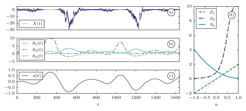
Figure 6. The summary of functions used to generate the non-stationary training data $X(t)$ according to the Eq. 5.3. a) The sample path of the process $X(t)$. b) The temporal evolution of the model parameters. c) The Parameter auxiliary process $u(t)$. d) The scaling functions $\theta_{n}(t)=S_{n}(u(t))$

.

Figure 6a demonstrates one realization of the sample path for the process $X(t)$. The SDE (5.3) is solved simultaneously with the Eq. (5.1) using different independent realizations of the Wiener process for each of the equations. We use the Euler-Maruyama method with a time-marching step size of $\Delta t=10^{-6}$ and then downsample the results to the time step $\Delta t=10^{-1}$, which then has in total $16384$ sample points. The scaling functions are defined as (see fig. 6d)

(5.4) $$\theta_{1}(t):=S_{1}(u) =2u(t)\,,$$

(5.5) $$\theta_{2}(t):=S_{2}(u) =\left[(u(t)-1)^{4}+0.1\right]^{-1}\,,$$

(5.6) $$\theta_{3}(t):=S_{3}(u) =(u(t)-1)^{2}+0.1\,.$$

The evolution of the vector $\bm{\Theta}(t)$ (see fig. 6b) and its functional relationship to the process $u(t)$ is hidden and supposed to be unknown in real applications. In this example, one can observe an interrelationship between the variance of the process $X(t)$ and the value of the process $u(t)$ by only considering the sample paths because the equation is linear. As shown in the next examples, this is not obvious with a nonlinear system. In the following, we demonstrate how the methodology introduced here is applied to recover the scaling functions $S_{n}$, given only the discrete-time values of $X(t)$ and $u(t)$. For details on running the optimization algorithm for this example see Appendix B.

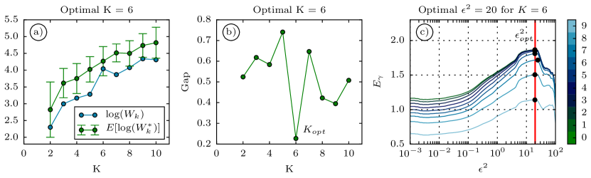
Figure 7. An estimation of the number of clusters for the OU example (see Fig. 6 and Eq. (5.3)) using the adapted gap statistics approach see Sect 3. In panel a) we find that for $K>6$ the diversity of the training data is increasing at the comparable rate as in the reference data sets. This suggest the optimal $K$ to be 6. This is confirmed by the minimum value in panel b). c) The estimation of the regularization parameter $\epsilon^{2}$ for the clustering with $K=6$. The colorbar codes the consecutive suppression of high frequency bands to emphasise the maximum. The effect is minimal.

By plotting the cluster averaged signal energy of the affiliation vector, i.e its $L_{2}$-norm, against the parameter $\epsilon^{2}$ we estimate the optimal value $\epsilon^{2}_{\textrm{opt}}$ for each value of $K$ individually (see one example for $K=6$ in fig. 7c). According to the figure 7c the maximum energy is found at a value $\epsilon^{2}_{\textrm{opt}}\approx 20$, which indicates the clearest separation of the regimes. As demonstrated in section 3.1 the maximum in the curve $E_{\gamma}$ may be further emphasized by suppressing the high frequencies in the vector $\bm{\Gamma}^{\ast}(t)$. This is highlighted in figure 7c with different colors, where index $0$ is the unfiltered result and each next integer marks the consecutive reduction of the frequency content by a factor of two (discrete wavelet transform). We find that the frequency suppression shows the desired effect, although this is unnecessary in this example because the maximum is well pronounced. Additionally, we have inspected the affiliation function for every value of $\epsilon^{2}$ (not shown) and found relatively small differences in its evolution for a wide range of the value $\epsilon^{2}$. This indicates a robust estimation and may be attributed to the simplicity of the example.

The procedure to estimate the optimal $K_{\textrm{opt}}$ requires more effort than it is the case with $\epsilon^{2}_{\textrm{opt}}$. We introduced the diversity measure in section 3.2 to characterize the incremental information gain with every additional cluster. Figure 7a demonstrates the graph of this measure (blue) for the training data $X(t)$ and for the reference data (green). The reference process is generated $B=20$ times with the same timestep that was used in the identification step. The clustering is repeated on each of these data sets with the value $\epsilon^{2}_{\textrm{opt}}\approx 20$ for each of the $K$ clusters. The intention is to keep all parameters of the framework unchanged and only to replace the data set. The resulting graph of the information gain for the clustering of the reference time series is shown in figure 7a (green). The key point to look for is the rate at which the information content is increased when clustering the analyzed data in comparison to the rate when clustering the reference time series.

Figure 7b shows the distance between the two clustering curves. A reasonable choice is $K_{\textrm{opt}}=6$ because afterwards the curve of the analyzed data does not approach the reference one, which means no significant further increase of the model diversity with respect to the reflected Wiener process. The expected value is built based on $10$ reference data sets. This number will be increased in the following examples to obtain better estimates.

Figure 8a displays $\bm{\Gamma}^{\ast}(t)$ obtained after clustering the time series $X(t)$ with $K=6$ (see Fig. 6a). The result is considered to be valid, since at almost every time instance we observe a high value of $\bm{\Gamma}^{\ast}(t)$ indicating a high certainty of the parameters. In Figure 8b the affiliation function is used to label the training data. Note, although the sample path of $X(t)$ at $t\approx 500$ appears to look similar to the sample path at $t\approx 1200$ the methodology is capable to differentiate a change in the parameters of the SDE and separate these times in two different clusters. This is attributed to the high accuracy of the method.

In Figure 8c the affiliation function is used to classify the auxiliary process $u(t)$. The regime occupation duration is changing across clusters. One can note that it is related to the rate of change of the auxiliary process. At times when this process is changing fast the occupation time is short and when the process is almost steady the regime occupation time is long. This observation highlights that the method is able to tract relatively rapid changes in the parameters if they occur frequently.

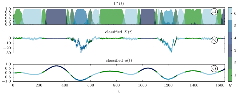
Figure 8. The result of clustering the example time series that is presented in Fig. 6. a) The affiliation function that is found in solving the variational problem Eq. (2.22) with $K=6$ and $\epsilon^{2}\approx 20$. b) The classified time series $X(t)$. c) The classified auxiliary process $u(t)$.

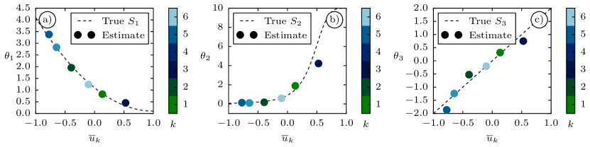
Figure 9. The estimated parameters plotted over the cluster averaged auxiliary process. The model identification is performed with an optimal number of clusters equal to six. The colorbar is labeling the different clusters as in Figure 8. The dots represent the estimated parameter values. The dashed line shows the true scaling functions, which were used in generating the training data.

Figure 9 shows the estimated parameters values for six clusters. The corresponding six points are sufficient to estimate the hidden scaling functions. When working with unexplored data the scaling functions would need to be parameterized from the scatter plots by applying a further regression analysis. We skip this step here because the estimated parameters are in a good agreement with the true functions. Parameter $\theta_{2}$ shows largest discrepancy in cluster $k=3$ (the right most point in fig. 9b) which is explained by the fact, that this cluster shows the largest variability of the process $u(t)$. Please observe the classified periods of $u(t)$ for $k=3$ in figure 8c. One way to improve the results would be to consider more sample points and repeat the clustering with more clusters.

5.3. SDE with Two Independent Auxiliary Processes

In this example, we consider an SDE with a nonlinear drift and a multiplicative noise term. Furthermore, the goal of this example is to demonstrate that the clustering methodology can handle modulation of two parameters which are independent and have different timescales. The following functional form of the SDE is investigated:

(5.7) $$\textrm{d}X=(2-\theta_{1}(t)X-\textrm{ln}(X^{2}))\textrm{d}t+\theta_{2}(t)X\textrm{d}W\,,\qquad X(t_{0})=1\,.$$

The relationship between the parameters and the auxiliary processes $u(t)$ and $v(t)$ is taken as

(5.8) $$\theta_{1}(t):=S_{1}(u) =(u(t)+1)^{4}+0.1\,,$$

(5.9) $$\theta_{2}(t):=S_{2}(v) =-2v(t)+2\,,$$

where $u(t)$ and $v(t)$ are independent solutions of Eq. (5.1) with different values for $T_{c}$: $T_{c,v}=4T_{c,u}$ (see Eq. (5.1)). The task is to recover the scaling functions solely from discrete-time observations of $X(t),u(t)$ and $v(t)$.For details on running the optimization algorithm for this example see Appendix C.

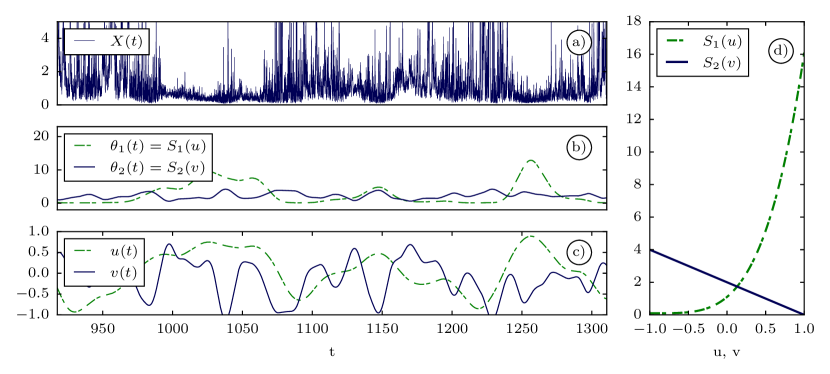
Figure 10. Summary of the functions to generate the non-stationary training data $X(t)$ according to the Eq. (5.7). a) The sample path of $X(t)$. b) The temporal evolution of the model parameters. c) The auxiliary parameter processes $u(t)$ and $v(t)$. d) The scaling functions $\theta_{n}(t)=S_{n}(u(t))$.

The sample size of the time series $X(t)$ is $131072$ ($\Delta t$ grid) points and it is longer than in the example with the OU process (see Sec. 5.2). More points support the methodology to distinguish the parameter variability. The processes $u(t)$ and $v(t)$ are uncorrelated and the re-occurrence of the unique parameter pairs in the sample path $X(t)$ is not assured. This makes the identification of the scaling functions ambitious. To mitigate the problem one needs to increase the number of clusters to raise the resolution of the scaling functions. By increasing the number of clusters we reduce the number of the samples available to estimate the parameter values within one cluster. Consequently, one also needs to increase the sample size of the total time series $X(t)$ to maintain the accuracy of the parameter estimates.

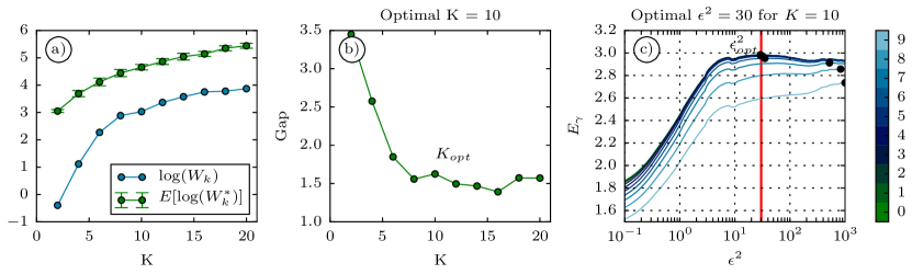
Figure 11. Estimation of the number of clusters for the example with two auxiliary processes (see Fig. (10) and Eq. (5.7)) using the gap statistics approach a) (see Eq. (3.9)) and b)(see Eq. (3.13)). In the panel a) after approximately $K=10$ the diversity of the training data is increasing at the same rate as in the reference data sets. This suggest the optimal $K$ to be around $10$. c) Estimation of the regularization parameter $\epsilon^{2}$ for clustering with $K=10$. The colorbar codes the consecutive suppression of high frequency bands to emphasize the maximum. The filtering step is not necessary in this example.

Figure 10a shows the sample path of the SDE (5.7) together with the auxiliary processes $u(t)$ and $v(t)$ (see Fig. 10c) which were used to generate $\bm{\Theta}(t)=[\theta_{1}(t),\theta_{2}(t)]$ (see Fig. 10b). The scaling functions are plotted in Fig. 11d.

The diversity measure of the clustering for the process $X(t)$ and the reference data set is shown for comparison in Fig. 11a. The peak in diversity when clustering the data set $X(t)$ is reached approximately at $K_{\textrm{opt}}=10$. By plotting the distance between the two curves we find that for $K>10$ the clustering does not add significantly more information relative to the clustering of the reflected Wiener process. The selection of $\epsilon^{2}_{\textrm{opt}}$ for this example shows a flat maximum (see Fig. 11c).

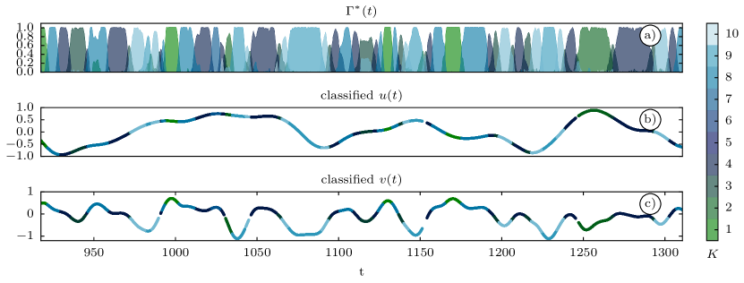
Figure 12. Result of the clustering the example time series that is presented in Fig. 10. a) The affiliation function that is found in solving the variational problem 2.22 with $K=10$ and $\epsilon^{2}=30$. b) The classified auxiliary process $u(t)$. c) The classified auxiliary process $v(t)$. The figure shows $30\%$ of the data set.

The optimal classifier $\bm{\Gamma}^{\ast}(t)$ and the partitioning of the auxiliary processes are shown in Fig. 12 where we can investigate the quality of the clustering. Figure 13 displays the estimated parameters and the true scaling functions. By visually inspecting these results we note a consistent spread of the estimates in the parameter $\theta_{2}$, but estimates in the parameter $\theta_{1}$ are distributed rather disproportionally. It is noticeable in the estimates of $\theta_{2}$ that three parameters have been apparently estimated twice and are positioned close to each other. The respective cluster values for the parameter $\theta_{1}$ however are located apart, such that the scaling function is sampled at significantly different points. This means that in this example the methodology is distinguishing pairs of parameters which have one common element. We therefore conclude that the methodology is capable to classify SDE models with at least two uncorrelated auxiliary processes.

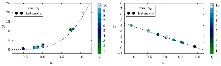
Figure 13. Estimated parameters plotted over the cluster averaged auxiliary processes. The model identification is performed with an optimal number of clusters equal to ten. The colorbar is labeling the different clusters as in Figure 8. The dots represent the estimated parameter values. The dashed line shows the true scaling functions, which were used in generating the training data.

In this example, we investigate an SDE with nonlinear drift and nonlinear diffusion. For the sake of simplicity, we consider only one auxiliary process $u(t)$ and two parameters: one in the drift term and one in the diffusion term. The functional form of the SDE is

(5.10) $$\textrm{d}X=(\theta_{1}(t)X-X^{3})\textrm{d}t+\theta_{2}(t)\sqrt{1+X^{2}}\textrm{d}W\,,\qquad X(t_{0})=0\,.$$

It is possible to incorporate more parameters into the model structure, for example, in front the quadratic or the cubic term. The parameter $\theta_{1}(t)$ is a time-dependent bifurcation parameter which causes a continuous variation of the equilibrium properties in time, eventually leading to metastable states in the dynamics. (see fig. 14a). The clustering methodology can comprehend transitions in the underlying double-well potential of the SDE. The relationship between the parameters and the auxiliary processes is

(5.11) $$\theta_{1}(t)\equiv S_{1}(u) =-0.4(u(t)-1)^{2}+2.5\,,$$

(5.12) $$\theta_{2}(t)\equiv S_{2}(u) =-4u(t)+5\,.$$

Like in the previous examples the task is to recover the scaling functions by only knowing one discrete-time trajectory of the process $X(t)$ and $u(t)$.

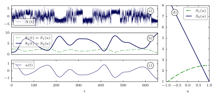
Figure 14. The example of a non-stationary process that is associated with Eq. (5.10). a) The sample path of $X(t)$. b) The temporal evolution of the model parameters. c) The parameter auxiliary process $u(t)$. d) The scaling functions $S_{n}(u(t))=\theta_{n}(t)$.

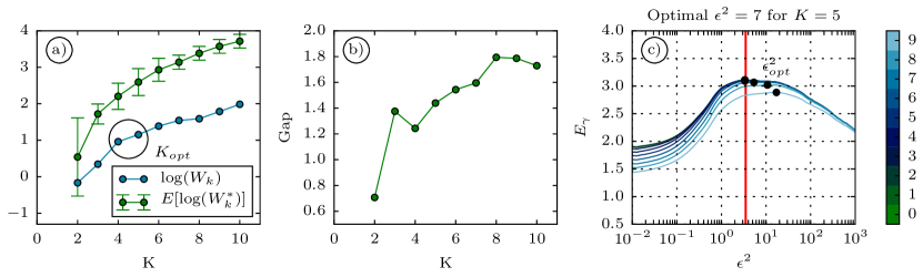
Figure 15. An estimation of the number of clusters for the example associated with Eq. (5.10) (see Fig. 14) using the gap statistics approach a) (see Eq. (3.9)) and b)(see Eq. (3.13)). In panel a) we find that for $K>4$ the diversity of the training data is increasing at constant rate. b) The gap statistics suggests $K_{opt}=4$. c) The estimation of the regularization parameter $\epsilon^{2}$ for clustering with $K=5$. The colorbar codes the consecutive suppression of high frequency bands to emphasize the maximum.

In this example our method to estimate $K_{\textrm{opt}}$ does not provide such a clear picture as it did in the previous examples. Nevertheless, it is still beneficial to analyze the tendencies of the curves in Figure 15a, b. As indicated by the minimum in the Figure 15b we should choose $K_{\textrm{opt}}=2$. However, our final goal is to recover the scaling functions and in the case of a nonlinear scaling functions one requires more than two points and therefore more clusters. According to the second minimum in Figure 15b, the second-best choice is $K_{\textrm{opt}}=4$. If we investigate the curve $\textrm{log}(W_{k})$ in Figure 15a, we find a minor characteristic change in the slope at $K_{\textrm{opt}}=4$. To resolve the scaling functions even better we select $K_{\textrm{opt}}=5$.

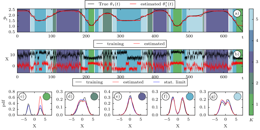
Figure 16. Clustered time series generated with Eq. (5.10). In a) and b) the colored background is the estimated affiliation vector $\bm{\Gamma}^{\ast}(t)>0.8$. The colorbar to the right of the panels labels the corresponding $5$ clusters. a) The true temporal evolution (black) of the drift parameter and its recovered version (red). Other values of the hyperparameters are given in Fig. 18. The second parameter looks similar and is not shown. b)The simulation of the sample path with the estimated parameter values compared to the training data. Panels c) to g) show the cluster respective densities: the histograms for the training (black) and simulation (red). The blue lines mark the stationary pdf which is computed from the parameter estimates. The colored circles are marking the corresponding clusters.

Knowing the affiliation function and the averaged values of the parameters, the temporal evolution of the model parameters (see Fig. 16a) is approximated by

(5.13) $$\theta^{\ast}(t)=\sum_{k=1}^{K_{\textrm{opt}}}\overline{\theta}^{\ast}_{k}\gamma_{k}(t)\,,$$

where $\overline{\theta}^{\ast}_{k}$ is a constant vector of size $N$. Figure 16a shows that the methodology recovers the hidden evolution of the parameters rather well. The approximation becomes better the more clusters are used (not shown). The drawback is that the uncertainty in $\overline{\bm{\Theta}}^{\ast}$ grows with the number of clusters, due to the reduction in data points per cluster.

The approximated path of the model parameters (see Fig. 16a in red) is used to test the prediction performance (see Fig. 16b in red). In this figure, the time series of the training dataset is shifted up for better comparison by the constant value of $10$. The considered SDE exhibits a temporal modulation by the bifurcation parameter. The times with two metastable states are expected to have different sample paths because the local state of the system is dependent on the particular realization of the Wiener process. Two different Wiener processes were used to generate the training and simulation solution. Figure 16b shows the properly captured signal dynamics. The corresponding cluster probability density functions are in good agreement with those of the training data and with the respective stationary distributions, which were computed from the parameter estimates. The largest discrepancy is shown for the cluster with index $1$ (see Fig. 16c). This cluster has a short lifetime to capture the regime jumping in the present realization. The trajectory-based p.d.f. estimate is off due to not observing the entire cluster dynamics. If we consider the stationary distribution computed from the estimated parameter values, we find the correct bimodal distribution (compare in Fig. 16c).

Figure 16 validates the performance of the model within the training data. To construct a self-contained, non-stationary prediction model, we show that the scaling functions between the auxiliary process $u(t)$ and the parameters are recovered as well (see Fig. 17).

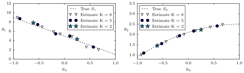
Figure 17. The estimated parameters plotted over the cluster averaged auxiliary process. The model identification is performed with an optimal number of clusters equal to six. The dots represent the estimated parameter values. The dashed line shows the true scaling functions, which were used in generating the training data. The optimal number of clusters is of second importance if one is able to parameterize the scaling functions.

The accuracy of the clustering method is sufficient to obtain the correct parameter values for a wide range of clusters used. It is important to note that the optimal number of clusters is of secondary importance. The number of clusters should be as low as possible and high enough to identify the scaling function. After the relation between the auxiliary process and the model parameter is identified ( see Fig. 17), the last step is consisting of performing a regression analysis to parameterize the scaling behavior. It is left out here as it will be specific for each application.

6. Discussion and Conclusion

Data-driven modeling has the ability to enhance the understanding of complex dynamical systems by highlighting patterns or hidden regularity. Especially challenging is the identification and the parameterization of nonlinear and non-stationary SDE. The intention of the system identification step is the determination of a suitable model structure and the estimation of the corresponding model parameters. In retrospect, one may analyze the data associated with the newly estimated model to improve understanding of the process to derive hidden relationships. These relationships may not be given explicitly by the clustering approach, so that unveiling these hidden dependencies requires additional research work. For instance, Vercauteren et al., (2016) characterized the influence of non-turbulent motions on the turbulence after a model-based data-clustering methodology was applied (Vercauteren and Klein,, 2015). In a study of the North Atlantic Oscillation in the climate system, Quinn et al., (2021) used the clustering results to study dynamical processes associated with atmospheric regime transitions.

The presented approach clusters the data into segments and models each of them with an individual, locally-stationary model. Such a decomposition of a complex dynamical behavior may not be optimal since it may not always be clear how to differentiate between a nonlinear and non-stationary time series without knowing the underlying structure of the data-generating process. Identifying an appropriate model structure is therefore an important step. For discrete-time systems, Billings, (2013) developed an estimation algorithm which can sequentially rate and collect important model terms. Following that, Wei et al., (2004) find an effective model for a highly nonlinear terrestrial magnetospheric dynamical system. Within their framework the time-varying parameters can be estimated with a multi-wavelet (Wei et al.,, 2010) or a sliding window approach (Li et al.,, 2016).

In section 2 we recall the variational clustering framework which allows the simultaneous analysis and modeling of a non-stationary time series. One variation of the framework (Horenko, 2010b, ) is based on discretized mathematical models, which are also termed discrete-time systems. To integrate an identified discrete-time model into a preexisting continuous-time system, one needs to account for the discretization operation, otherwise, the solution is restricted to the time frequency given by the data. One way to overcome the problem is to convey the frequency response of the identified model by transforming it into a continuous one (Kuznetsov and Clarke,, 1994). This transformation is widely studied in linear system theory and is extendable for the case of nonlinear systems (Billings,, 2013)[p. 342]. Our approach avoids the above-mentioned difficulty because we use the MLE derived from an appropriate likelihood (fitness) function for the discrete-time observations of SDE.

In general, the main challenge in applying the MLE is the missing transition density function, which requires, for example, a solution of the Fokker-Plank equation for a considered structure of the SDE. Especially for the nonlinear SDE, this function is analytically not known and demands estimation (Fuchs,, 2013). In our approach, by separating the available time series into $K$ clusters, the available number of samples for estimation reduces, leading thereby to uncertain estimates in each of them. The closed-form approximation based on the Hermite expansion provides an accurate approximation for the transition density, with an error of $O(\Delta t^{4})$ (Ait-Sahalia,, 2002). This accuracy allows to increase the number of clusters and to raise the resolution of the hidden scaling functions making an accurate parameterization task feasible.

We combine the closed-form likelihood function approach based on suitable Hermite-expansions with the non-parametric clustering framework. Specifically, we highlight the details of the necessary modification in the original subspace clustering algorithm to achieve accurate estimates of the model parameters independently of the discretization of the QP problem. Furthermore, we present an extensive numerical study consisting of three controlled examples of different complexity to validate both the parameterization methodology and the novel methods to estimate the hyperparameters of the framework, which are independent and does not rely on information theory.

In particular, our approach to estimating the optimal number of clusters is based on measuring the degree of model diversity and comparing it to the clustering of the reflected reference Wiener process. The numerical experiments confirm that this approach produces adequately reliable estimates. However, the associated graphs prove to be dependent on the considered model structure such that the selection requires a case-specific interpretation. The proposed method is still computationally expensive because it requires to repeat the clustering of the reference data set multiple times to construct an expected value.

Our method to identify the optimal regularization value of the affiliation function proves to be robust for the studied test cases. We further extended it to articulate the optimum through consecutively filtering out the small-scale variability from the affiliation vector. Unfortunately, we could not construct an appropriated example to show its potential. However, apart from this study, we tested this methodology on the real-data application and found it to be effective. This will be reported in a follow-up study.

In summary, the data-driven variational clustering approach enables modeling of the nonlinear and non-stationary processes to develop models for multi-scale dynamical systems. The model structure of the SDE is thereby unknown and demands to be prescribed or inferred in supplementary ways. The parameterization method is accurate and provides reasonable results with small data sets consisting of $2\times 10^{4}$ points. It is also scalable on the GPU as it is realized in this work. We tested data sets consisting of $2\times 10^{6}$ points, where the computation time was approximately 24 hours on a GeForce 1080 with 3 clusters. The numerical examples demonstrate the correct identification of the required scaling functions, which allows parameterizing a considered SDE by linking additional auxiliary processes to the model parameters.

This work focuses on one-dimensional time series; however, it is possible to extend the approach to a multi-dimensional case. One should consider following two research directions. The first one is to use the closed-form likelihood expansion for multivariate diffusion (Aït-Sahalia,, 2008). Modification of the variational clustering method is not required for this. However, practically one may run into problems of over-parameterization because the cross-dimensional interaction terms and their temporal variability lead to unconstrained systems. One way to mitigate this is to enforce diagonally-spars diffusion and drift matrices as it is demonstrated by O’Kane et al., (2017).

The second research direction is to examine multi-dimensional or even spatial problems. Then it is suggestible to replace the MLE with an ensemble Kalman inversion method (Albers et al.,, 2019). The variational clustering framework is also generalized to classify the spatial parameter variability (Kaiser,, 2015, p. 81). Pospisil et al., (2018) implemented this approach within the openly available code, which is linked in their work. The proposed methods appear promising, however with increasing dimensions, it becomes more and more important to estimate the correct functional terms rather than the parameter values. Hence, an additional inverse problem may be combined with the presented approach to assessing the structural form of the system.

Finally, it is noteworthy that the presented parameterization method is intended to be used to develop a data-driven stochastic parameterization of intermittent turbulence present in the nocturnal atmospheric boundary layer. In climate models for example, the limited numerical resolution leaves unresolved degrees of freedom, commonly denoted as subgrid-scale processes. The approach presented here provides an ideal framework to derive subgrid-scale models which are modulated by resolved variables. These results will be published elsewhere. Another direction for future research is the extension of the non-stationary data-driven learning approach developed in this work to SDE models with (at least) two widely separated time scales, for which the MLE is known to become asymptotically biased. For these systems the proposed methodology has to be combined with multiscale robust inference techniques (Krumscheid et al.,, 2013; Kalliadasis et al.,, 2015; Krumscheid,, 2018).

Appendix A Reusing of the initial guess

One can estimate the values of the hyperparameters $K$ and $\epsilon^{2}$ by running the optimization problem for each pair of parameter combinations. In the OU example, we choose for $K$ the range of values $[2,3,\dots,10]$ and for $\epsilon^{2}$ the range of values $[10^{-1},10^{2}]$, where we use $100$ divisions on the logarithmic scale for the latter one. In principle for each parameter combination $(K,\epsilon^{2})$ the optimization method can be started with a random initial guess $\overline{\bm{\Theta}}_{0}$ and $\bm{\Gamma}_{0}(t)$. However, practically it is efficient to use the optimal values from the previous run in the following way:

1. Select one value for $K$,

2. Initialize the first optimization run with the smallest or the largest value of $\epsilon^{2}_{0}$ together with a random guess for $\overline{\bm{\Theta}}_{0}$ and $\bm{\Gamma}_{0}(t)$,

3. Algorithm 1 provides a solution $\overline{\bm{\Theta}}^{\ast}_{1}$ and $\bm{\Gamma}^{\ast}_{1}$

4. Change the parameter value $\epsilon^{2}$ to the next closest value $\epsilon^{2}_{1}$,

5. Start the optimization method with $\epsilon^{2}_{1}$ and the initial guess to be the solution from the previous run: $\overline{\bm{\Theta}}^{\ast}_{1}$ and $\bm{\Gamma}^{\ast}_{1}$,

6. Algorithm 1 provides to the solution $\overline{\bm{\Theta}}^{\ast}_{2}$ and $\bm{\Gamma}^{\ast}_{2}$,

7. Solve the variational problem for all considered $\epsilon^{2}$ by incrementally changing its value,

8. Change the value of $K$ and repeat with (1).

The approach where the initial guess is taken randomly requires , of course, more computational time in total than the case with reused solution of previous simulations. The principle of traversing the regularization parameter $\epsilon^{2}$ is further exploited by traversing the parameter from low to high value and back to a low value while consistently reusing the previous solution outcomes. This strategy showed to be effective to find a better solution after each iteration, although with only minor incremental improvement.

Appendix B Details on the settings of the framework for the OU example in section 5.3

The minimization algorithm for the QP solver has two stopping criteria which are as follows. The maximum number of iterations is set to $100$, and the minimum difference between consecutive cost function values is set to $10^{-8}$. The reduction value for the QP solver speeds up the QP problem and is set to $1/3$. For the $\bm{\Theta}$ solver, the global optimizer is a random search algorithm supplemented with a local search algorithm. For both of them, the maximum number of function evaluations is set to $300$ and the break tolerance to a relative value $10^{-10}$. The population size of the global optimizer is set to $3000$. The final point to mention is the parameter bounds for the $\bm{\Theta}$ solver. In this example (and for the clustering of the reference data set) they are :$-20<\theta_{1}<20;\ 0<\theta_{2}<20;\ 0<\theta_{3}<20$.

Appendix C Details on the settings of the framework for the example in Section 5.4

Here are the details on the simulation of the sample path $X(t)$ (see Fig. 14) which forms the training data for the clustering test. The time series $X(t)$ has $65536$ samples and a constant time step $\Delta t=0.01$. The sample path is obtained by solving the Eq. 5.10 with the Milstein method and the sample path of $u(t)$ is obtained by solving the Eq. 5.1 with the Euler-Maruyama method. During the simulation the time step between each of the $65536$ samples is reduced to the the value $10^{-4}$ in order to obtain a more accurate realization of the sample path. The initial value for Eq. 5.10 is set to $X(t_{0})=0$ and for Eq. 5.1 - to $U(t_{0})=[1,0,0,0]$. The parameters in Eq. 5.1 were taken to be $T_{c}=15$; $b_{0}=0.2$.

Next we provide the details on parameters of the clustering framework itself. In this example, the maximum number of iteration is set to $100$ and the minimum difference in the consecutive evaluation of the fitness function is set to a relative value $10^{-8}$. The reduction value for the $\bm{\Gamma}$ solver is set to $\alpha=0.1$. For both of solvers, the maximum number of calls is set to $500$ and the termination tolerance to a relative value $10^{-10}$. The population size of the global optimizer is set to $1000$. The bounds for the parameter limits of the $\bm{\Theta}$ solver (and for the clustering of the reference data set) is:$-10<\theta_{1}<10;\ 0<\theta_{2}<10$.

Appendix D Coefficients of the Hermit Expansion

The coefficients $\eta_{j}$ in Eq. (2.9) are approximated with a truncated Taylor series of length $M=J/2$ , where $J=6$. We state them here for completeness.

$$\begin{split}\eta_{0}^{(3)}&=1\;,\\ \eta_{1}^{(3)}&=-\mu{h}^{1/2}-\frac{2\mu\mu^{\prime}+\mu^{\prime\prime}}{4}{h}^{3/2}-\frac{4\mu{\mu^{\prime}}^{2}+4{\mu}^{2}\mu^{\prime\prime}+6\mu^{\prime}\mu^{\prime\prime}+4\mu\mu^{(3)}+\mu^{(4)}}{24}{h}^{5/2}\;,\\ \eta_{2}^{(3)}&=\frac{{\mu}^{2}+\mu^{\prime}}{2}h+\frac{6{\mu}^{2}\mu^{\prime}+4{(\mu^{\prime})}^{2}+7\mu\mu^{\prime\prime}+2\mu^{(3)}}{12}{h}^{2}+\frac{1}{96}\Bigl{(}28{\mu}^{2}{(\mu^{\prime})}^{2}+28{\mu}^{2}\mu^{(3)}\\ &\quad+16{(\mu^{\prime})}^{3}+16{\mu}^{3}{\mu^{\prime\prime}}+88\mu\mu^{\prime}\mu^{\prime\prime}+21{(\mu^{\prime\prime})}^{2}+32\mu^{\prime}\mu^{(3)}+16\mu\mu^{(4)}+3\mu^{(5)}\Bigr{)}{h}^{3}\;,\\ \eta_{3}^{(3)}&=-\frac{{\mu}^{3}+3\mu\mu^{\prime}+\mu^{\prime\prime}}{6}{h}^{3/2}-\frac{1}{48}\Bigl{(}12{\mu}^{3}\mu^{\prime}+28\mu{(\mu^{\prime})}^{2}+22{\mu}^{2}\mu^{\prime\prime}+24\mu^{\prime}\mu^{\prime\prime}\\ &\quad+14\mu\mu^{(3)}+3\mu^{(4)}\Bigr{)}{h}^{5/2}\;,\\ \eta_{4}^{(3)}&=\frac{{\mu}^{4}+6{\mu}^{2}\mu^{\prime}+3{(\mu^{\prime})}^{2}+4\mu\mu^{\prime\prime}+\mu^{(3)}}{24}{h}^{2}+\frac{1}{240}\Bigl{(}20{\mu}^{4}\mu^{\prime}+50{\mu}^{3}\mu^{\prime\prime}+100{\mu}^{2}{(\mu^{\prime})}^{2}\\ &\quad+50{\mu}^{2}\mu^{(3)}+23\mu\mu^{(4)}+180\mu\mu^{\prime}\mu^{\prime\prime}+40{(\mu^{\prime})}^{3}+34{(\mu^{\prime\prime})}^{2}+52\mu^{\prime}\mu^{(3)}+4\mu^{(5)}\Bigr{)}{h}^{3}\;,\\ \eta_{5}^{(3)}&=-\frac{{\mu}^{5}+10{\mu}^{3}\mu^{\prime}+15\mu{(\mu^{\prime})}^{2}+10{\mu}^{2}\mu^{\prime\prime}+10\mu^{\prime}\mu^{\prime\prime}+5\mu\mu^{(3)}+\mu^{(4)}}{120}{h}^{5/2}\;,\\ \eta_{6}^{(3)}&=\frac{1}{720}\Bigl{(}{\mu}^{6}+15{\mu}^{4}\mu^{\prime}+15{(\mu^{\prime})}^{3}+20{\mu}^{3}\mu^{\prime\prime}+15\mu^{\prime}\mu^{(3)}+45{\mu}^{2}{(\mu^{\prime})}^{2}+10{(\mu^{\prime\prime})}^{2}\\ &\quad+15{\mu}^{2}\mu^{(3)}+60\mu\mu^{\prime}\mu^{\prime\prime}+6\mu\mu^{(4)}+\mu^{(5)}\Bigr{)}{h}^{3}\;,\end{split}$$

where $\mu$ is the drift of the $Y$ process evaluated at $y_{0}$ (see Eq. (2.8)), ”^′” denotes a derivative and $h=\Delta t$. The Hermite polynomials for our expansion are: $H_{0}(z)=1,H_{1}(z)=-z,H_{2}(z)=-1+z^{2},H_{3}(z)=3z-z^{3},H_{4}(z)=3-6z^{2}+z^{4},H_{5}(z)=-15z+10z^{3}-z^{5},H_{6}(z)=-15+45z^{2}-15z^{4}+z^{6}$.

Appendix E Variation of the Hyperparameters

The section contains a sensitivity analysis to demonstrate different solution options of the clustering frame work.

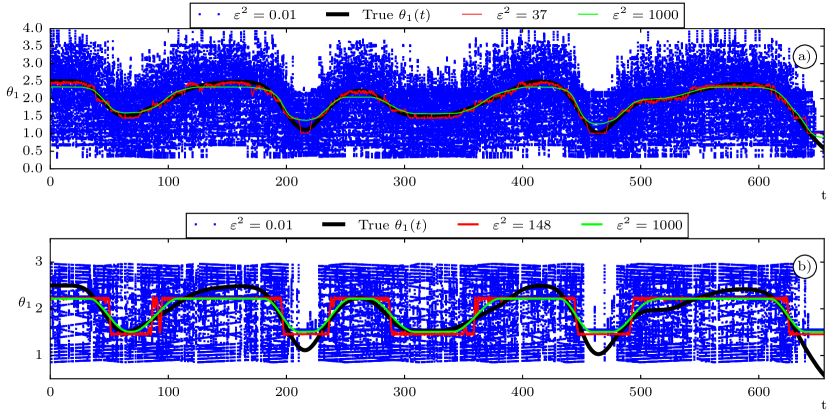
Figure 18. Reconstruction of the hidden evolution of one parameter for the nonlinear SDE using different values of the two significant hyperparameters ($K$ and $\varepsilon^{2}$). Panel a) shows the parameter reconstructed with eight clusters and panel b) using two clusters. Highly scattered blue dots label the weakly regularized solution. The red curves are suggested as an optimal value following the presented approach.

References

- Ait-Sahalia, (1999) Ait-Sahalia, Y. (1999). Transition Densities for Interest Rate and Other Nonlinear Diffusions. The Journal of Finance, page 35.
- Ait-Sahalia, (2002) Ait-Sahalia, Y. (2002). Maximum Likelihood Estimation of Discretely Sampled Diffusions: A Closed-form Approximation Approach. Econometrica, 70(1):223–262.
- Albers et al., (2019) Albers, D. J., Blancquart, P.-A., Levine, M. E., Esmaeilzadeh Seylabi, E., and Stuart, A. (2019). Ensemble Kalman methods with constraints. Inverse Problems, 35(9):095007.
- Ayenew et al., (2009) Ayenew, T., Fikre, S., Wisotzky, F., Demlie, M., and Wohnlich, S. (2009). Hierarchical cluster analysis of hydrochemical data as a tool for assessing the evolution and dynamics of groundwater across the Ethiopian rift. page 15.
- Aït-Sahalia, (2008) Aït-Sahalia, Y. (2008). Closed-form likelihood expansions for multivariate diffusions. The Annals of Statistics, 36(2).
- Billings, (2013) Billings, S. A. (2013). Nonlinear system identification: NARMAX methods in the time, frequency, and spatio-temporal domains. John Wiley & Sons, Inc, Chichester, West Sussex, United Kingdom.
- Boyko and Vercauteren, (2020) Boyko, V. and Vercauteren, N. (2020). Multiscale Shear Forcing of Turbulence in the Nocturnal Boundary Layer: A Statistical Analysis. Boundary-Layer Meteorology.
- Dacunha-Castelle and Florens-Zmirou, (1986) Dacunha-Castelle, D. and Florens-Zmirou, D. (1986). Estimation of the coefficients of a diffusion from discrete observations. Stochastics, 19(4):263–284.
- de Wiljes et al., (2013) de Wiljes, J., Majda, A., and Horenko, I. (2013). An Adaptive Markov Chain Monte Carlo Approach to Time Series Clustering of Processes with Regime Transition Behavior. Multiscale Modeling & Simulation, 11(2):415–441.
- Foufoula-Georgiou and Kumar, (1994) Foufoula-Georgiou, E. and Kumar, P., editors (1994). Wavelets in geophysics. Number v. 4 in Wavelet analysis and its applications. Academic Press, San Diego.
- Franzke et al., (2015) Franzke, C. L. E., O’Kane, T. J., Monselesan, D. P., Risbey, J. S., and Horenko, I. (2015). Systematic attribution of observed Southern Hemisphere circulation trends to external forcing and internal variability. Nonlinear Processes in Geophysics, 22(5):513–525.
- Fuchs, (2013) Fuchs, C. (2013). Inference for Diffusion Processes. Springer Berlin Heidelberg, Berlin, Heidelberg.
- G. Johnson, (2021) G. Johnson, S. (2021). The NLopt nonlinear-optimization package.
- Gerber and Horenko, (2014) Gerber, S. and Horenko, I. (2014). On inference of causality for discrete state models in a multiscale context. Proceedings of the National Academy of Sciences, 111(41):14651–14656.
- (15) Horenko, I. (2010a). Finite Element Approach to Clustering of Multidimensional Time Series. SIAM Journal on Scientific Computing, 32(1):62–83.
- (16) Horenko, I. (2010b). On the Identification of Nonstationary Factor Models and Their Application to Atmospheric Data Analysis. Journal of the Atmospheric Sciences, 67(5):1559–1574.
- Horenko et al., (2020) Horenko, I., Marchenko, G., and Gagliardini, P. (2020). On a computationally scalable sparse formulation of the multidimensional and nonstationary maximum entropy principle. Communications in Applied Mathematics and Computational Science, 15(2):129–146. Publisher: Mathematical Sciences Publishers.
- Horsthemke, (1984) Horsthemke, W. (1984). Noise Induced Transitions. Non-Equilibrium Dynamics in Chemical Systems, pages 150–160. Publisher: Springer, Berlin, Heidelberg.
- Kaelo and Ali, (2006) Kaelo, P. and Ali, M. M. (2006). Some Variants of the Controlled Random Search Algorithm for Global Optimization. Journal of Optimization Theory and Applications, 130(2):253–264.
- Kaiser, (2015) Kaiser, O. (2015). Data-based analysis of extreme events: inference, numerics and applications. PhD thesis, Università della Svizzera italiana.
- Kaiser et al., (2017) Kaiser, O., Hien, S., Achatz, U., and Horenko, I. (2017). Stochastic Subgrid-Scale Pa- rametrization. page 1.
- Kaiser and Horenko, (2014) Kaiser, O. and Horenko, I. (2014). On inference of statistical regression models for extreme events based on incomplete observation data. Communications in Applied Mathematics and Computational Science, 9(1):143–174.
- Kalliadasis et al., (2015) Kalliadasis, S., Krumscheid, S., and Pavliotis, G. A. (2015). A new framework for extracting coarse-grained models from time series with multiscale structure. J. Comput. Phys., 296:314–328.
- Krumscheid, (2018) Krumscheid, S. (2018). Perturbation-based inference for diffusion processes: Obtaining effective models from multiscale data. Math. Models Methods Appl. Sci., 28(8):1565–1597.
- Krumscheid et al., (2013) Krumscheid, S., Pavliotis, G. A., and Kalliadasis, S. (2013). Semiparametric Drift and Diffusion Estimation for Multiscale Diffusions. Multiscale Model. Simul., 11(2):442–473.
- Krumscheid et al., (2015) Krumscheid, S., Pradas, M., Pavliotis, G. A., and Kalliadasis, S. (2015). Data-driven coarse graining in action: Modeling and prediction of complex systems. Physical Review E, 92(4):042139.
- Kuznetsov and Clarke, (1994) Kuznetsov, A. and Clarke, D. (1994). Simple Numerical Algorithms for Continuous-To-Discrete and Discrete-To-Continuous Conversion of the Systems with Time Delay. IFAC Proceedings Volumes, 27(8):1549–1554.
- Lee et al., (2019) Lee, G., Gommers, R., Waselewski, F., Wohlfahrt, K., and O’Leary, A. (2019). PyWavelets: A Python package for wavelet analysis. Journal of Open Source Software, 4(36):1237.
- Li et al., (2016) Li, Y., Wei, H.-L., Billings, S. A., and Sarrigiannis, P. (2016). Identification of nonlinear time-varying systems using an online sliding-window and common model structure selection (CMSS) approach with applications to EEG. International Journal of Systems Science, 47(11):2671–2681.
- Liao, (2005) Liao, T. W. (2005). Clustering of time series data—a survey. Pattern Recognition, page 18.
- Mahrt, (2014) Mahrt, L. (2014). Stably Stratified Atmospheric Boundary Layers. Annual Review of Fluid Mechanics, 46(1):23–45.
- Maione et al., (2019) Maione, C., Nelson, D. R., and Barbosa, R. M. (2019). Research on social data by means of cluster analysis. Applied Computing and Informatics, 15(2):153–162.
- Metzner et al., (2012) Metzner, P., Putzig, L., and Horenko, I. (2012). Analysis of persistent nonstationary time series and applications. Communications in Applied Mathematics and Computational Science, 7(2):175–229.
- O’Kane et al., (2013) O’Kane, T. J., Risbey, J. S., Franzke, C., Horenko, I., and Monselesan, D. P. (2013). Changes in the Metastability of the Midlatitude Southern Hemisphere Circulation and the Utility of Nonstationary Cluster Analysis and Split-Flow Blocking Indices as Diagnostic Tools. Journal of the Atmospheric Sciences, 70:19.
- O’Kane et al., (2017) O’Kane, T. J., Monselesan, D. P., Risbey, J. S., Horenko, I., and Franzke, C. L. E. (2017). Research Article. On memory, dimension, and atmospheric teleconnections. Mathematics of Climate and Weather Forecasting, 3(1):1–27.
- O’Kane et al., (2016) O’Kane, T. J., Risbey, J. S., Monselesan, D. P., Horenko, I., and Franzke, C. L. E. (2016). On the dynamics of persistent states and their secular trends in the waveguides of the Southern Hemisphere troposphere. Climate Dynamics, 46(11-12):3567–3597.
- Pospisil et al., (2018) Pospisil, L., Gagliardini, P., Sawyer, W., and Horenko, I. (2018). On a scalable nonparametric denoising of time series signals. Communications in Applied Mathematics and Computational Science, 13(1):107–138.
- Price, (1977) Price, W. L. (1977). A controlled random search procedure for global optimisation. The Computer Journal, 20(4):367–370.
- Price, (1983) Price, W. L. (1983). Global optimization by controlled random search. Journal of Optimization Theory and Applications, 40(3):333–348.
- Putzig et al., (2010) Putzig, L., Becherer, D., and Horenko, I. (2010). Optimal Allocation of a Futures Portfolio Utilizing Numerical Market Phase Detection. SIAM Journal on Financial Mathematics, 1(1):752–779.
- Quinn et al., (2021) Quinn, C., Harries, D., and O’Kane, T. J. (2021). Dynamical analysis of a reduced model for the North Atlantic Oscillation. Journal of the Atmospheric Sciences. Publisher: American Meteorological Society.
- Richard P, (2013) Richard P, B. (2013). Algorithms for minimization without derivatives. Courier Corporation.
- Risbey et al., (2015) Risbey, J. S., O’Kane, T. J., Monselesan, D. P., Franzke, C., and Horenko, I. (2015). Metastability of Northern Hemisphere Teleconnection Modes. Journal of the Atmospheric Sciences, 72(1):35–54.
- Sun et al., (2012) Sun, J., Mahrt, L., Banta, R. M., and Pichugina, Y. L. (2012). Turbulence Regimes and Turbulence Intermittency in the Stable Boundary Layer during CASES-99. Journal of the Atmospheric Sciences, 69(1):338–351. Publisher: American Meteorological Society.
- Tibshirani et al., (2001) Tibshirani, R., Walther, G., and Hastie, T. (2001). Estimating the number of clusters in a data set via the gap statistic. Journal of the Royal Statistical Society: Series B (Statistical Methodology), 63(2):411–423.
- Vercauteren et al., (2019) Vercauteren, N., Boyko, V., Kaiser, A., and Belusic, D. (2019). Statistical Investigation of Flow Structures in Different Regimes of the Stable Boundary Layer. Boundary-Layer Meteorology, 173(2):143–164.
- Vercauteren and Klein, (2015) Vercauteren, N. and Klein, R. (2015). A Clustering Method to Characterize Intermittent Bursts of Turbulence and Interaction with Submesomotions in the Stable Boundary Layer. Journal of the Atmospheric Sciences, 72(4):1504–1517.
- Vercauteren et al., (2016) Vercauteren, N., Mahrt, L., and Klein, R. (2016). Investigation of interactions between scales of motion in the stable boundary layer: Interactions between Scales of Motion in the Stable Boundary Layer. Quarterly Journal of the Royal Meteorological Society, 142(699):2424–2433.
- Wei et al., (2004) Wei, H. L., Billings, S. A., and Liu, J. (2004). Term and variable selection for non-linear system identification. International Journal of Control, 77(1):86–110.
- Wei et al., (2010) Wei, H. L., Billings, S. A., and Liu, J. J. (2010). Time-varying parametric modelling and time-dependent spectral characterisation with applications to EEG signals using multiwavelets. International Journal of Modelling, Identification and Control, 9(3):215.
- Yuan and Yang, (2019) Yuan, C. and Yang, H. (2019). Research on K-Value Selection Method of K-Means Clustering Algorithm. J, 2(2):226–235.
- Zhao and Karypis, (2005) Zhao, Y. and Karypis, G. (2005). Data Clustering in Life Sciences. Molecular Biotechnology, 31(1):055–080.