Automated Discovery of Adaptive Attacks on Adversarial Defenses

Abstract

Reliable evaluation of adversarial defenses is a challenging task, currently limited to an expert who manually crafts attacks that exploit the defense’s inner workings or approaches based on an ensemble of fixed attacks, none of which may be effective for the specific defense at hand. Our key observation is that adaptive attacks are composed of reusable building blocks that can be formalized in a search space and used to automatically discover attacks for unknown defenses. We evaluated our approach on 24 adversarial defenses and show that it outperforms AutoAttack (Croce & Hein, 2020b), the current state-of-the-art tool for reliable evaluation of adversarial defenses: our tool discovered significantly stronger attacks by producing 3.0%-50.8% additional adversarial examples for 10 models, while obtaining attacks with slightly stronger or similar strength for the remaining models.

1 Introduction

The issue of adversarial attacks (Szegedy et al., 2014; Goodfellow et al., 2015), i.e., crafting small input perturbations that lead to mispredictions, is an important problem with a large body of recent work. Unfortunately, reliable evaluation of proposed defenses is an elusive and challenging task: many defenses seem to initially be effective, only to be circumvented later by new attacks designed specifically with that defense in mind (Carlini & Wagner, 2017; Athalye et al., 2018; Tramer et al., 2020).

To address this challenge, two recent works approach the problem from different perspectives. Tramer et al. (2020) outlines an approach for manually crafting adaptive attacks that exploit the weak points of each defense. Here, a domain expert starts with an existing attack, such as PGD (Madry et al., 2018) (denoted as $\bullet$ in Figure 1), and adapts it based on knowledge of the defense’s inner workings. Common modifications include: (i) tuning attack parameters (e.g., number of steps), (ii) replacing network components to simplify the attack (e.g., removing randomization or non-differentiable components), and (iii) replacing the loss function optimized by the attack. This approach was demonstrated to be effective in breaking all of the considered $13$ defenses. However, a downside is that it requires substantial manual effort and is limited by the domain knowledge of the expert – for instance, each of the $13$ defenses came with an adaptive attack which was insufficient, in retrospect.

At the same time, Croce & Hein (2020b) proposed to assess adversarial robustness using an ensemble of four attacks illustrated in Figure 1 (b) – APGD${}_{\texttt{CE}}$ with cross-entropy loss (Croce & Hein, 2020b), APGD${}_{\texttt{DLR}}$ with difference in logit ratio loss, FAB (Croce & Hein, 2020a), and SQR (Andriushchenko et al., 2020). While these do not require manual effort and have been shown to improve the robustness estimate for many defenses, the approach is inherently limited by the fact that the attacks are fixed apriori without any knowledge of the given defense at hand. This is visualized in Figure 1 (b) where even though the attacks are designed to be diverse, they cover only a small part of the entire space.

Figure 1: High-level illustration and comparison of recent works and ours. Adaptive attacks (a) rely on a human expert to manually adapt an existing attack to exploit the weak points of each defense. AutoAttack (b) evaluates defenses using an ensemble of diverse attacks. Our work (c) defines a search space of adaptive attacks (denoted as ) and performs search steps automatically.

This work: towards automated discovery of adaptive attacks

We present a new method that helps automating the process of crafting adaptive attacks, combining the best of both prior approaches; the ability to evaluate defenses automatically while producing attacks tuned for the given defense. Our work is based on the key observation that we can identify common techniques used to build existing adaptive attacks and extract them as reusable building blocks in a common framework. Then, given a new model with an unseen defense, we can discover an effective attack by searching over suitable combinations of these building blocks. To identify reusable techniques, we analyze existing adaptive attacks and organize their components into three groups:

• Attack algorithm and parameters: a library of diverse attack techniques (e.g., APGD, FAB, C&W (Carlini & Wagner, 2017), NES (Wierstra et al., 2008)), together with backbone specific and generic parameters (e.g., input randomization, number of steps, if/how to use EOT (Athalye et al., 2018)).

• Network transformations: producing an easier to attack surrogate model using techniques including variants of BPDA (Athalye et al., 2018) to break gradient obfuscation, and layer removal (Tramer et al., 2020) to eliminate obfuscation layers such as redundant softmax operator.

• Loss functions: that specify different ways of defining the attack’s loss function.

These components collectively formalize an attack search space induced by their different combinations. We also present an algorithm that effectively navigates the search space so to discover an attack. In this way, domain experts are left with the creative task of designing new attacks and growing the framework by adding missing attack components, while the tool is responsible for automating many of the tedious and time-consuming trial-and-error steps that domain experts perform manually today. That is, we can automate some part of the process of finding adaptive attacks, but not necessarily the full process. This is natural as finding truly new attacks is a highly creative process that is currently out of reach for fully automated techniques.

We implemented our approach in a tool called Adaptive AutoAttack (A³) and evaluated it on $24$ diverse adversarial defenses. Our results demonstrate that A³ discovers adaptive attacks that outperform AutoAttack (Croce & Hein, 2020b), the current state-of-the-art tool for reliable evaluation of adversarial defenses: A³ finds attacks that are significantly stronger, producing 3.0%-50.8% additional adversarial examples for 10 models, while obtaining attacks with stronger or simialr strength for the remaining models. Our tool A³ and scripts for reproducing the experiments are available online at:

https://github.com/eth-sri/adaptive-auto-attack

2 Automated Discovery of Adaptive Attacks

We use $\mathcal{D}=\{(x_{i},y_{i})\}_{i=1}^{N}$ to denote a training dataset where $x\in{\mathbb{X}}$ is a natural input (e.g., an image) and $y$ is the corresponding label. An adversarial example is a perturbed input $x^{\prime}$, such that: (i) it satisfies an attack criterion $c$, e.g., a $K$-class classification model $f\colon{\mathbb{X}}\rightarrow{\mathbb{R}}^{K}$ predicts a wrong label, and (ii) the distance $d(x^{\prime},x)$ between the adversarial input $x^{\prime}$ and the natural input $x$ is below a threshold $\epsilon$ under a distance metric $d$ (e.g., an $L_{p}$ norm). Formally, this can be written as:

For example, instantiating this with the $L_{\infty}$ norm and misclassification criterion corresponds to:

where $\hat{f}$ returns the prediction $\operatorname*{arg\,max}_{k=1:K}f_{k}(\cdot)$ of the model $f$.

Problem Statement

Given a model $f$ equipped with an unknown set of defenses and a dataset $\mathcal{D}=\{(x_{i},y_{i})\}_{i=1}^{N}$, our goal is to find an adaptive adversarial attack $a\in{\mathcal{A}}$ that is best at generating adversarial samples $x^{\prime}$ according to the attack criterion $c$ and the attack capability $d(x^{\prime},x)\leq\epsilon$:

$$\max_{a\in{\mathcal{A}},~{}d(x^{\prime},x)\leq\epsilon}\mathbb{E}_{(x,y)\sim\mathcal{D}}\quad c(f,x^{\prime},x)\qquad\qquad\text{where}\quad x^{\prime}=a(x,f)$$ (1)

Here, ${\mathcal{A}}$ denotes the search space of all possible attacks, where the goal of each attack $a\colon{\mathbb{X}}\times({\mathbb{X}}\rightarrow{\mathbb{R}}^{K})\rightarrow{\mathbb{X}}$ is to generate an adversarial sample $x^{\prime}=a(x,f)$ for a given input $x$ and model $f$. For example, solving this optimization problem with respect to the $L_{\infty}$ misclassification criterion corresponds to optimizing the number of adversarial examples misclassified by the model.

In our work, we consider an implementation-knowledge adversary, who has full access to the model’s implementation at inference time (e.g., the model’s computational graph). We chose this threat model as it matches our problem setting – given an unseen model implementation, we want to automatically find an adaptive attack that exploits its weak points but without the need of a domain expert. We note that this threat model is weaker than a perfect-knowledge adversary (Biggio et al., 2013), which assumes a domain expert that also has knowledge about the training dataset and algorithm, as this information is difficult, or even not possible, to recover from the model’s implementation only.

Key Challenges

To solve the optimization problem from Eq. 1, we address two key challenges:

• Defining a suitable attacks search space ${\mathcal{A}}$ such that it is expressible enough to cover a range of existing adaptive attacks.

• Searching over the space ${\mathcal{A}}$ efficiently such that a strong attack is found within a reasonable time.

Next, we formalize the attack space in Section 3 and then describe our search algorithm in Section 4.

3 Adaptive Attacks Search Space

We define the adaptive attack search space by analyzing existing adaptive attacks and identifying common techniques used to break adversarial defenses. Formally, the adaptive attack search space is given by ${\mathcal{A}}\colon{\mathbb{S}}\times{\mathbb{T}}$, where ${\mathbb{S}}$ consists of sequences of backbone attacks along with their loss functions, selected from a space of loss functions ${\mathbb{L}}$, and ${\mathbb{T}}$ consists of network transformations. Semantically, given an input $x$ and a model $f$, the goal of adaptive attack $(s,t)\in{\mathbb{S}}\times{\mathbb{T}}$ is to return an adversarial example $x^{\prime}$ by computing $s(x,t(f))=x^{\prime}$. That is, it first transforms the model $f$ by applying the transformation $t(f)=f^{\prime}$, and then executes the attack $s$ on the surrogate model $f^{\prime}$. Note that the surrogate model is used only to compute the candidate adversarial example, not to evaluate it. That is, we generate an adversarial example $x^{\prime}$ for $f^{\prime}$, and then check whether it is also adversarial for $f$. Since $x^{\prime}$ may be adversarial for $f^{\prime}$, but not for $f$, the adaptive attack must maximize the transferability of the generated candidate adversarial samples.

Attack Algorithm & Parameters (${\mathbb{S}}$)

The attack search space consists of a sequence of adversarial attacks. We formalize the search space with the grammar:

(Attack Search Space)
$\qquad{\mathbb{S}}$ ::=	${\mathbb{S}}$; ${\mathbb{S}}$ $\mid$ $\mathtt{randomize}$ ${\mathbb{S}}$ $\mid$ $\mathtt{EOT}$ ${\mathbb{S}}$, n $\mid$ $\mathtt{repeat}$ ${\mathbb{S}}$, n $\mid$
	$\mathtt{try}$ ${\mathbb{S}}$ $\mathtt{for}$ n $\mid$ Attack $\mathtt{with}$ params $\mathtt{with}$ loss $\in{\mathbb{L}}$

• ${\mathbb{S}};~{}{\mathbb{S}}$: composes two attacks, which are executed independently and return the first adversarial sample in the defined order. That is, given input $x$, the attack $s_{1};s_{2}$ returns $s_{1}(x)$ if $s_{1}(x)$ is an adversarial example, and otherwise it returns $s_{2}(x)$.

• $\mathtt{randomize}$ ${\mathbb{S}}$: enables the attack’s randomized components, which correspond to random seed and/or selecting a starting point within $~{}d(x^{\prime},x)\leq\epsilon$, uniformly at random.

• $\mathtt{EOT}$ ${\mathbb{S}}$, n: uses expectation over transformation, a technique designed to compute gradients for models with randomized components (Athalye et al., 2018).

• $\mathtt{repeat}$ ${\mathbb{S}}$, n: repeats the attack $n$ times (useful only if randomization is enabled).

• $\mathtt{try}$ ${\mathbb{S}}$ $\mathtt{for}$ n: executes the attack with a time budget of n seconds.

• Attack $\mathtt{with}$ params $\mathtt{with}$ loss $\in{\mathbb{L}}$: is a backbone attack Attack executed with parameters params and loss function loss. In our evaluation, we use FGSM (Goodfellow et al., 2015), PGD, DeepFool (Moosavi-Dezfooli et al., 2016), C&W, NES, APGD, FAB and SQR. We provide full list of the attack parameters, including their ranges and priors in Appendix B.

Note, that we include variety of backbone attacks, including those that were already superseeded by stronger attacks. This is done for two key reasons. First, weaker attacks can be surprisingly effective in some cases and avoid the detector because of their weakness (see defense C24 in our evaluation). Second, we are not using any prior when designing the space search. In particular, whenever a new attack is designed it can simply be added to the search space. Then, the goal of the search algorithm is to be powerful enough to perform the search efficiently. In other words, the aim is to avoid making any assumptions of what is useful or not and let the search algorithm learn this instead.

Network Transformations (${\mathbb{T}}$)

A common approach that aims to improve the robustness of neural networks against adversarial attacks is to incorporate an explicit defense mechanism in the neural architecture. These defenses often obfuscate gradients to render iterative-optimization methods ineffective (Athalye et al., 2018). However, these defenses can be successfully circumvented by (i) choosing a suitable attack algorithm, such as score and decision-based attacks (included in ${\mathbb{S}}$), or (ii) by changing the neural architecture (defined next).

At a high level, the network transformation search space ${\mathbb{T}}$ takes as input a model $f$ and transforms it to another model $f^{\prime}$, which is easier to attack. To achieve this, the network $f$ can be expressed as a directed acyclic graph, including both the forward and backward computations, where each vertex denotes an operator (e.g., convolution, residual blocks, etc.), and edges correspond to data dependencies. In our work, we include two types of network transformations:

Layer Removal, which removes an operator from the graph. Each operator can be removed if its input and output dimensions are the same, regardless of its functionality.

Backward Pass Differentiable Approximation (BPDA) (Athalye et al., 2018), which replaces the backward version of an operator with a differentiable approximation of the function. In our search space we include three different function approximations: (i) an identity function, (ii) a convolution layer with kernel size 1, and (iii) a two-layer convolutional layer with ReLU activation in between. The weights in the latter two cases are learned through approximating the forward function.

Loss Function (${\mathbb{L}}$)

Selecting the right objective function to optimize is an important design decision for creating strong adaptive attacks. Indeed, the recent work of Tramer et al. (2020) uses 9 different objective functions to break 13 defenses, showing the importance of this step. We formalize the space of possible loss functions using the following grammar:

(Loss Function Search Space)
${\mathbb{L}}$ ::=	$\mathtt{targeted}$ Loss, n $\mathtt{with}$ Z $\mid$ $\mathtt{untargeted}$ Loss $\mathtt{with}$ Z $\mid$
	$\mathtt{targeted}$ Loss, n - $\mathtt{untargeted}$ Loss $\mathtt{with}$ Z
Z ::=	logits $\mid$ probs
Loss ::=	CrossEntropy $\mid$ HingeLoss $\mid$ L1 $\mid$ DLR $\mid$ LogitMatching

Targeted vs Untargeted. The loss can be either untargeted, where the goal is to change the classification to any other label $f(x^{\prime})\neq f(x)$, or targeted, where the goal is to predict a concrete label $f(x^{\prime})=l$. Even though the untargeted loss is less restrictive, it is not always easier to optimize in practice, and replacing it with a targeted attack might perform better. When using $\mathtt{targeted}$ Loss, n, the attack will consider the top n classes with the highest probability as the targets.

Loss Formulation. The concrete loss formulation includes loss functions used in existing adaptive attacks, as well as the recently proposed difference in logit ratio loss (Croce & Hein, 2020b). We provide a formal definition of the loss functions used in our work in Appendix B.

Logits vs. Probabilities. In our search space, loss functions can be instantiated both with logits as well as with probabilities. Note that some loss functions are specifically designed for one of the two options, such as C&W (Carlini & Wagner, 2017) or DLR (Croce & Hein, 2020b). While such knowledge can be used to reduce the search space, it is not necessary as long as the search algorithm is powerful enough to recognize that such a combination leads to poor results.

Loss Replacement. Because the key idea behind many of the defenses is finding a property that helps differentiate between adversarial and natural images, one can also define the optimization objective in the same way. These feature-level attacks (Sabour et al., 2016) avoid the need to directly optimize the complex objective defined by the adversarial defense and have been effective at circumventing them. As an example, the logit matching loss minimizes the difference of logits between adversarial sample $x^{\prime}$ and a natural sample of the target class $x$ (selected at random from the dataset). Instead of logits, the same idea can also be applied to other statistics, such as internal representations computed by a pre-trained model or KL-divergence between label probabilities.

4 Search Algorithm

We now describe our search algorithm that optimizes the problem statement from Eq. 1. Since we do not have access to the underlying distribution, we approximate Eq. 1 using the dataset $\mathcal{D}$ as follows:

$$\textstyle score(f,a,\mathcal{D})=\frac{1}{\lvert\mathcal{D}\rvert}\sum_{i=1}^{\lvert\mathcal{D}\rvert}-\lambda l_{a}+\max_{d(x^{\prime},x)\leq\epsilon}c(f,a(x,f),x)$$ (2)

where $a\in{\mathcal{A}}$ is an attack, $l_{a}\in{\mathbb{R}}^{+}$ denotes untargeted cross-entropy loss of $a$ on the input, and $\lambda\in{\mathbb{R}}$ is a hyperparameter. The intuition behind $-\lambda\cdot l_{a}$ is that it acts as a tie-breaker in case the criterion $c$ alone is not enough to differentiate between multiple attacks. While this is unlikely to happen when evaluating on large datasets, it is quite common when using only a small number of samples. Obtaining good estimates in such cases is especially important for achieving scalability since performing the search directly on the full dataset would be prohibitively slow.

1

2

def AdaptiveAttackSearch

       Input: dataset $\mathcal{D}$, model $f$, attack search space ${\mathcal{A}}={\mathbb{S}}\times{\mathbb{T}}$, number of trials $k$, initial dataset size $n$, attack sequence length $m$, criterion function $c$, initial parameter estimator model $M$, default attack $\Delta\in{\mathbb{S}}$

       Output: adaptive attack from $a_{[s,t]}\in{\mathcal{A}}={\mathbb{S}}\times{\mathbb{T}}$ achieving the highest $score$ on $\mathcal{D}$

3       $t\leftarrow\operatorname*{arg\,max}_{t\in{\mathbb{T}}}score(f,a_{[\Delta,t]},\mathcal{D})$ $\triangleright$ Find surrogate model $t$ using default attack $\Delta$

4       ${\mathcal{S}}\leftarrow\bot$ $\triangleright$ Initialize attack to be no attack, which returns the input image

5       for $j\leftarrow 1\!:\!m$ do $\triangleright$ Run $m$ iterations to get sequence of $m$ attacks

6             $\mathcal{D}\leftarrow\mathcal{D}\setminus\{x\mid x\in\mathcal{D}\wedge c(f,a_{[{\mathcal{S}},t]}(x,f),x)\}$ $\triangleright$ Remove non-robust samples

7             ${\mathcal{H}}\leftarrow\emptyset;~{}\mathcal{D}_{\texttt{sample}}\leftarrow sample(\mathcal{D},n)$ $\triangleright$ Initial dataset with $n$ samples

8             for $i\leftarrow 1\!:\!k$ do $\triangleright$ Select candidate adaptive attacks

9                   $\theta^{\prime}\leftarrow\operatorname*{arg\,max}_{\theta\in{\mathbb{S}}}P(\theta\mid M)$ $\triangleright$ Best unseen parameters according to the model $M$

10                   $q\leftarrow score(f,a_{[\theta^{\prime},t]},\mathcal{D}_{\texttt{sample}})$

11                   ${\mathcal{H}}\leftarrow{\mathcal{H}}\cup\{(\theta^{\prime},q)\}$

12                   $M\leftarrow$ update model $M$ with $(\theta^{\prime},q)$

13                  

14            ${\mathcal{H}}\leftarrow$ keep $\lvert{\mathcal{H}}\rvert/4$ attacks with the best score

15             while $\lvert{\mathcal{H}}\rvert>1~{}\textbf{and}~{}\mathcal{D}_{\texttt{sample}}\neq\mathcal{D}$ do $\triangleright$ Successive halving (SHA)

16                   $\mathcal{D}_{\texttt{sample}}\leftarrow\mathcal{D}_{\texttt{sample}}\cup sample(\mathcal{D}\setminus\mathcal{D}_{\texttt{sample}},\lvert\mathcal{D}_{\texttt{sample}}\rvert)$ $\triangleright$ Double the dataset size

17                   ${\mathcal{H}}\leftarrow\{(\theta,score(f,a_{[\theta,t]},\mathcal{D}_{\texttt{sample}}))\mid(\theta,q)\in{\mathcal{H}}\}$ $\triangleright$ Re-evaluate on larger dataset

18                   ${\mathcal{H}}\leftarrow$ keep $\lvert{\mathcal{H}}\rvert/4$ attacks with the best score

19                  

20            ${\mathcal{S}}\leftarrow{\mathcal{S}};~{}$best attack in ${\mathcal{H}}$

21      return $a_{[{\mathcal{S}},t]}$

Algorithm 1 A search algorithm that given a model $f$ with unknown defense, discovers an adaptive attack from the attack search space ${\mathcal{A}}$ with the best $score$.

Search Algorithm

We present our search algorithm in Algorithm 1. We start by searching through the space of network transformations $t\!\in\!{\mathbb{T}}$ to find a suitable surrogate model (line 1). This is achieved by taking the default attack $\Delta$ (in our implementation, we set $\Delta$ to APGD${}_{\texttt{CE}}$), and then evaluating all locations where BPDA can be used, and subsequently evaluating all layers that can be removed. Even though this step is exhaustive, it takes only a fraction of the runtime in our experiments, and no further optimization was necessary.

Next, we search through the space of attacks ${\mathbb{S}}$. As this search space is enormous, we employ three techniques to improve scalability and attack quality. First, to generate a sequence of $m$ attacks, we perform a greedy search (lines 3-16). That is, in each step, we find an attack with the best score on the samples not circumvented by any of the previous attacks (line 4). Second, we use a parameter estimator model $M$ to select the suitable parameters (line 7). In our work, we use Tree of Parzen Estimators (Bergstra et al., 2011), but the concrete implementation can vary. Once the parameters are selected, they are evaluated using the $score$ function (line 8), the result is stored in the trial history ${\mathcal{H}}$ (line 9), and the estimator is updated (line 10). Third, because evaluating the adversarial attacks can be expensive, and the dataset $\mathcal{D}$ is typically large, we employ successive halving technique (Karnin et al., 2013; Jamieson & Talwalkar, 2016). Concretely, instead of evaluating all the trials on the full dataset, we start by evaluating them only on a subset of samples $\mathcal{D}_{\texttt{sample}}$ (line 5). Then, we improve the score estimates by iteratively increasing the dataset size (line 13), re-evaluating the scores (line 14), and retaining a quarter of the trials with the best score (line 15). We repeat this process to find a single best attack from ${\mathcal{H}}$, which is then added to the sequence of attacks ${\mathcal{S}}$ (line 16).

Time Budget and Worst-case Search Time

We set a time budget on the attacks, measured in seconds per sample per attack, to restrict resource-expensive attacks and allow the tradeoff between computation time and attack strength. If an attack exceeds the time limit in line 8, the evaluation terminates, and the score is set to be $-\infty$. We analyzed the worst-case search time to be $4/3\times$ the allowed attack runtime in our experiments, which means the search overhead is both controllable and reasonable in practice. The derivation is shown in Appendix A.

5 Evaluation

We evaluate A³ on 24 models with diverse defenses and compare the results to AutoAttack (Croce & Hein, 2020b) and to several existing handcrafted attacks. AutoAttack is a state-of-the-art tool designed for reliable evaluation of adversarial defenses that improved the originally reported results for many existing defenses by up to 10%. Our key result is that A³ finds stronger or similar attacks than AutoAttack for virtually all defenses:

• In 10 cases, the attacks found by A³ are significantly stronger than AutoAttack, resulting in 3.0% to 50.8% additional adversarial examples.

• In the other 14 cases, A³’s attacks are typically 2x faster while enjoying similar attack quality.

Model Selection

We selected 24 models and divided them into three blocks A, B, C as listed in Table 1. Block A contains diverse defenses with $\epsilon=4/255$. Block B contains selected top models from RobustBench  (Croce et al., 2020). Block C contains diverse defenses with $\epsilon=8/255$.

The A³ tool

The implementation of A³ is based on PyTorch (Paszke et al., 2019), the implementations of FGSM, PGD, NES, and DeepFool are based on FoolBox (Rauber et al., 2017) version 3.0.0, C&W is based on ART (Nicolae et al., 2018) version 1.3.0, and the attacks APGD, FAB, and SQR are from (Croce & Hein, 2020b). We use AutoAttack’s rand version if a defense has a randomization component, and otherwise we use its standard version. To allow for a fair comparison, we extended AutoAttack with backward pass differential approximation (BPDA), so we can run it on defenses with non-differentiable components; without this, all gradient-based attacks would fail. We instantiate Algorithm 1 by setting: the attack sequence length $m=3$, the number of trials $k=64$, the initial dataset size $n=100$, and we use a time budget of $0.5$ to $3$ seconds per sample depending on the model size. All of the experiments are performed using a single RTX 2080 Ti GPU.

Table 1: Comparison of AutoAttack (AA) and our approach (A³) on 24 defenses. Further details of each defense, discovered adaptive attacks and confidence intervals are included in Appendix D and H.

		Robust Accuracy (1 - Rerr)				Runtime (min)				Search
CIFAR-10, $l_{\infty}$, $\epsilon=4/255$		AA	A3	$\quad\Delta\quad$		AA	A3	Speed-up		A3
A1	Madry et al. (2018)	44.78	44.69	-0.09		25	20	1.25$\times$		88
A2†	Buckman et al. (2018)	2.29	1.96	-0.33		9	7	1.29$\times$		116
A3†	Das et al. (2017) + Lee et al. (2018)	0.59	0.11	-0.48		6	2	3.00$\times$		40
A4	Metzen et al. (2017)	6.17	3.04	-3.13		21	13	1.62$\times$		80
A5	Guo et al. (2018)	22.30	12.14	-10.16		19	17	1.12$\times$		99
A6†	Pang et al. (2019)	4.14	3.94	-0.20		28	24	1.17$\times$		237
A7	Papernot et al. (2015)	2.85	2.71	-0.14		4	4	1.00$\times$		84
A8	Xiao et al. (2020)	19.82	11.11	-8.71		49	22	2.23$\times$		189
A9	Xiao et al. (2020)${}_{\texttt{ADV}}$	64.91	63.56	-1.35		157	100	1.57$\times$		179
A9’	Xiao et al. (2020)${}_{\texttt{ADV}}$	64.91	17.70	-47.21		157	2,280	0.07$\times$		1,548
CIFAR-10, $l_{\infty}$, $\epsilon=8/255$
B10∗	Gowal et al. (2021)	62.80	62.79	-0.01		818	226	3.62$\times$		761
B11∗	Wu et al. (2020)${}_{\texttt{RTS}}$	60.04	60.01	-0.03		706	255	2.77$\times$		690
B12∗	Zhang et al. (2021)	59.64	59.56	-0.08		604	261	2.31$\times$		565
B13∗	Carmon et al. (2019)	59.53	59.51	-0.02		638	282	2.26$\times$		575
B14∗	Sehwag et al. (2020)	57.14	57.16	0.02		671	429	1.56$\times$		691
CIFAR-10, $l_{\infty}$, $\epsilon=8/255$
C15∗	Stutz et al. (2020)	77.64	39.54	-38.10		101	108	0.94$\times$		296
C15’	Stutz et al. (2020)	77.64	26.87	-50.77		101	205	0.49$\times$		659
C16∗	Zhang & Wang (2019)	36.74	37.11	0.37		381	302	1.26$\times$		726
C17	Grathwohl et al. (2020)	5.15	5.16	0.01		107	114	0.94$\times$		749
C18	Xiao et al. (2020)${}_{\texttt{ADV}}$	5.40	2.31	-3.09		95	146	0.65$\times$		828
C19	Wang et al. (2019)	50.84	50.81	-0.03		734	372	1.97$\times$		755
C20†	B11 + Defense in A3	60.72	60.04	-0.68		621	210	2.96$\times$		585
C21†	C17 + Defense in A3	15.27	5.24	-10.03		261	79	3.30$\times$		746
C22	B11 + Random Rotation	49.53	41.99	-7.54		255	462	0.55$\times$		900
C23	C17 + Random Rotation	22.29	13.45	-8.84		114	374	0.30$\times$		1,023
C24	Hu et al. (2019)	6.25	3.07	-3.18		110	56	1.96$\times$		502
∗model available from the authors, †model with non-differentiable components.
B12 uses $\epsilon=0.031$. C15 uses $\epsilon=0.03$. A9’ uses time budget $T_{c}=30$. C15’ uses $m=8$.

Evaluation Metric

Following Stutz et al. (2020), we use the robust test error (Rerr) metric to combine the evaluation of defenses with and without detectors. We include details in Appendix C. In our evaluation, A³ produces consistent results on the same model across independent runs with the standard deviation $\sigma<0.2$ (computed across 3 runs). The details are included in Appendix H.

Comparison to AutoAttack

Our main results, summarized in Table 1, show the robust accuracy (lower is better) and runtime of both AutoAttack (AA) and A³ over the 24 defenses. For example, for A8 our tool finds an attack that leads to lower robust accuracy (11.1% for A³ vs. 19.8% for AA) and is more than twice as fast (22 min for A³ vs. 49 min for AA). Overall, A³ significantly improves upon AA or provides similar but faster attacks.

We note that the attacks from AA are included in our search space (although without the knowledge of their best parameters and sequence), and so it is expected that A³ performs at least as well as AA, provided sufficient exploration time. Importantly, A³ often finds better attacks: for 10 defenses, A³ reduces the robust accuracy by 3% to 50% compared to AA. Next, we discuss the results in more detail.

Defenses based on Adversarial Training. Models in block B are selected from RobustBench (Croce et al., 2020), and they are based on various extensions of adversarial training, such as using additional unlabelled data for training, extensive hyperparameter tuning, instance weighting or loss regularization. The results show that the robustness reported by AA is already very high and using A³ leads to only marginal improvement. However, because our tool also optimizes for the runtime, A³ does achieve significant speed-ups, ranging from 1.5$\times$ to 3.6$\times$. The reasons behind the marginal robustness improvement of A³ are two-fold. First, it shows that A³ is limited by the attack techniques search space, as the attack found are all variations of APGD. Second, the models B10 - B14 aim to improve the adversarial training procedure rather than developing a new defence. This is in contrast to models that do design various types of new defences (included in blocks A and C), evaluating which typically requires discovering a new adaptive attack. For these new defences, evaluation is much more difficult and this is where our approach also improves the most.

Obfuscation Defenses. Defenses A3, A8, A9, C18, C20, and C21 are based on gradient obfuscation. A³ discovers stronger attacks that reduce the robust accuracy for all defenses by up to 47.21%. Here, removing the obfuscated defenses in A3, C20, and C21 provides better gradient estimation for the attacks. Further, the use of more suitable loss functions strengthens the discovered attacks and improves the evaluation results for A8 and C18.

Randomized Defenses. For the randomized input defenses A8, C22, and C23, A³ discovers attacks that, compared to AA’s rand version, further reduce robustness by 8.71%, 7.54%, and 8.84%, respectively. This is achieved by using stronger yet more costly parameter settings, attacks with different backbones (APGD, PGD) and 7 different loss functions (as listed in Appendix D).

Detector based Defenses. For C15, A4, and C24 defended with detectors, A³ improves over AA by reducing the robustness by 50.77%, 3.13%, and 3.18%, respectively. This is because none of the attacks discovered by A³ are included in AA. Namely, A³ found SQR${}_{\texttt{DLR}}$ and APGD${}_{\texttt{Hinge}}$ for C15, untargeted FAB for A4 (FAB in AA is targeted), and PGD${}_{\texttt{L1}}$ for C24.

Generalization of A³

Given a new defense, the main strength of our approach is that it directly benefits from all existing techniques included in the search space. Here, we compare our approach to three handcrafted adaptive attacks not included in the search space.

As a first example, C15 (Stutz et al., 2020) proposes an adaptive attack PGD-Conf with backtracking that leads to robust accuracy of 36.9%, which can be improved to 31.6% by combining PGD-Conf with blackbox attacks. A³ finds APGD${}_{\texttt{Hinge}}$ and Z = probs. This combination is interesting since the hinge loss maximizing the difference between the top two predictions, in fact, reflects the PGD-Conf objective function. Further, similarly to the manually crafted attack by C15, a different blackbox attack included in our search space, SQR${}_{\texttt{DLR}}$, is found to complement the strength of APGD. When using a sequence of three attacks, we achieve 39.54% robust accuracy. We can decrease the robust accuracy even further by increasing the number of attacks to eight – the robust accuracy drops to 26.87%, which is a stronger result than the one reported in the original paper. In this case, our search space and the search algorithm are powerful enough to not only replicate the main ideas of Stutz et al. (2020) but also to improve its evaluation when allowing for a larger attack budget. Note that this improvement is possible even without including the backtracking used by PGD-Conf as a building block in our search space. In comparison, the robust accuracy reported by AA is only 77.64%.

As a second example, C18 is known to be susceptible to NES which achieves 0.16% robust accuracy (Tramer et al., 2020). To assess the quality of our approach, we remove NES from our search space and instead try to discover an adaptive attack using the remaining building blocks. In this case, our search space was expressive enough to find an alternative attack that achieves 2.31% robust accuracy.

As a third example, to break C24, Tramer et al. (2020) designed an adaptive attack that linearly interpolates between the original and the adversarial samples using PGD. This technique breaks the defense and achieves 0% robust accuracy. In comparison, we find PGD${}_{\texttt{L1}}$, which achieves 3.07% robust accuracy. In this case, the fact that PGD${}_{\texttt{L1}}$ is a relatively weak attack is an advantage – it successfully bypasses the detector by not generating overconfident predictions.

A³ Interpretability

As illustrated above, it is possible to manually analyze the discovered attacks in order to understand how they break the defense mechanism. Further, we can also gain insights from the patterns of attacks searched across all the models (shown in Appendix D, Table 6). For example, it turns out that $\ell_{\texttt{CE}}$ is not as frequent as $\ell_{\texttt{DLR}}$ or $\ell_{\texttt{hinge}}$. This fact challenges the common practice of using $\ell_{\texttt{CE}}$ as the default loss when evaluating robustness. In addition, using $\ell_{\texttt{CE}}$ during adversarial training can make models resilient to $\ell_{\texttt{CE}}$, loss, but not necessarily to other losses.

A³ Scalability

To assess A³’s scalability, we perform two ablation studies: (i) increase the search space by $4\times$ (by adding $8$ random attacks, their corresponding parameters, and $4$ dummy losses), and (ii) keep the search space size unchanged but reduce the search runtime by half. In (i), we observed a marginal performance decrease when using the same runtime, and we can reach the same attack strength when the runtime budget is increased by $1.5\times$. In (ii), even when we reduce the runtime by half, we can still find attacks that are only slightly worse ($\leq 0.4$). This shows that a budget version of the search can provide a strong robustness evaluation. We include detailed results in Appendix E.

Ablation Studies

Similar to existing handcrafted adaptive attacks, all three components included in the search space were important for generating strong adaptive attacks for a variety of defenses. Here we briefly discuss their importance while including the full experiment results in Appendix F.

Attack & Parameters. We demonstrate the importance of parameters by comparing PGD, C&W, DF, and FGSM with default library parameters to the best configuration found when available parameters are included in the search space. The attacks found by A³ are on average 5.5% stronger than the best attack among the four attacks on A models.

Loss Formulation. To evaluate the effect of modeling different loss functions, we remove them from the search space and keep only the original loss function defined for each attack. The search score drops by 3% on average for A models without the loss formulation.

Table 2: The robust accuracy (1 - Rerr) of networks with different BPDA policies evaluated by APGD${}_{\texttt{CE}}$ with 50 iterations.

BPDA Type	A2	A3	C20	C21
identity	18.5	9.6	70.5	84.0
1x1 convolution	8.9	10.3	70.8	84.9
2 layer conv+ReLU	3.7	14.9	74.1	86.2

Network Processing. In C21, the main reason for achieving 10% decrease in robust accuracy is the removal of the gradient obfuscated defense Reverse Sigmoid. We provide a more detailed ablation in Table 2, which shows the effect of different BPDA instantiations included in our search space. For A2, since the non-differentiable layer is non-linear thermometer encoding, it is better to use a function with non-linear activation to approximate it. For A3, C20, C21, the defense is image JPEG compression and identity network is the best algorithm since the networks can overfit when training on limited data.

6 Related Work

The most closely related work to ours is AutoAttack (Croce & Hein, 2020b), which improves the evaluation of adversarial defenses by proposing an ensemble of four fixed attacks. Further, the key to stronger attacks was a new algorithm APGD, which improves upon PGD by halving the step size dynamically based on the loss at each step. In our work, we improve over AutoAttack in three keys aspects: (i) we formalize a search space of adaptive attacks, rather than using a fixed ensemble, (ii) we design a search algorithm that discovers the best adaptive attacks automatically, significantly improving over the results of AutoAttack, and (iii) our search space is extensible and allows reusing building blocks from one attack by other attacks, effectively expressing new attack instantiations. For example, the idea of dynamically adapting the step size is not tied to APGD, but it is a general concept applicable to any step-based algorithm.

Another related work is Composite Adversarial Attacks (CAA) (Mao et al., 2021). The main idea of CAA is that instead of selecting an ensemble of four attacks that complement each other as done by AutoAttack, the authors proposed to search for a sequence of attacks that achieve the best performance. Here, the authors focus on evaluating defences based on adversarial training and show improvements of up to 1% over AutoAttack. In comparison, our main idea is that the way adaptive attacks are designed today can be formalized as a search space that includes not only sequence of attacks but also loss functions, network processing and rich space of hyperparameters. This is critical as it defines a much larger search space to cover a wide range of defenses, beyond the reach of both CA and AutoAttack. This can be also seen in our evaluation – we achieve significant improvement by finding 3% to 50% more adversarial examples for 10 models.

Our work is also closely related to the recent advances in AutoML, such as in the domain of neural architecture search (NAS) (Zoph & Le, 2017; Elsken et al., 2019). Similar to our work, the core challenge in NAS is an efficient search over a large space of parameters and configurations, and therefore many techniques can also be applied to our setting. This includes BOHB (Falkner et al., 2018), ASHA (Li et al., 2018), using gradient information coupled with reinforcement learning (Zoph & Le, 2017) or continuous search space formulation (Liu et al., 2019). Even though finding completely novel neural architectures is often beyond the reach, NAS is still very useful and finds many state-of-the-art models. This is also true in our setting – while human experts will continue to play a key role in defining new types of adaptive attacks, as we show in our work, it is already possible to automate many of the intermediate steps.

7 Conclusion

We presented the first tool that aims to automate the process of finding strong adaptive attacks specifically tailored to a given adversarial defense. Our key insight is that we can identify reusable techniques used in existing attacks and formalize them into a search space. Then, we can phrase the challenge of finding new attacks as an optimization problem of finding the strongest attack over this search space.

Our approach automates the tedious and time-consuming trial-and-error steps that domain experts perform manually today, allowing them to focus on the creative task of designing new attacks. By doing so, we also immediately provide a more reliable evaluation of new and existing defenses, many of which have been broken only after their proposal because the authors struggled to find an effective attack by manually exploring the vast space of techniques. Importantly, even though our current search space contains only a subset of existing techniques, our evaluation shows that A³ can partially re-discover or even improve upon some handcrafted adaptive attacks not included in our search space.

However, there are also limitations to overcome in future work. First, while the search space can be easily extended, it is also inherently incomplete, and domain experts will still play an important role in designing novel types of attacks. Second, the search algorithm does not model the attack runtime and as a result, incorporating expensive attacks can be computational unaffordable. This is problematic as it can incur huge overhead even if a fast attack does exist. Finally, an interesting future work is to use meta-learning to improve the search even further, allowing A³ to learn across multiple models, rather than starting each time from scratch.

8 Societal Impacts

In this paper, an approach to improve the evaluation of adversarial defenses by automatically finding adaptive adversarial attacks is proposed and evaluated. As such, this work builds on a large body of existing research on developing adversarial attacks and defences and thus shares the same societal impacts. Concretely, the presented approach can be used both in a beneficial way by the researchers developing adversarial defenses, as well as, in a malicious way by an attacker trying to break existing models. In both cases, the approach is designed to improve empirical model evaluation, rather than providing verified model robustness, and thus is not intended to provide formal robustness guarantees for safety-critical applications. For applications where formal robustness guarantess are required, instead of using empirical techniques as in this work, one should instead adapt the concurrent line of work on certified robustness.

Appendix A A³ Time Complexity

This section gives the worst-case time analysis for Algorithm 1. We denote $T_{a}$ to be the attack time and $T_{r}$ to be the search time. We will show that with the per sample per attack time constraint of $T_{c}$:

$$T_{a}\leq m\times N\times T_{c}$$ (3)

$$T_{r}\leq 2\times m\times n\times k\times T_{c}$$ (4)

Where $m$, $N$, $n$, $k$ are the number of attacks, the size of the dataset $D$, the size of initial dataset size, the number of attacks to sample respectively.

In Algorithm 1, only steps on lines 1,4,8,14 are timing critical as they apply the expensive attack algorithms. Other steps like sampling datasets and applying parameter estimator $M$ are considered as constant overhead. $T_{a}$ is the total runtime of line 4, because line 4 is the step to apply the attack on all the samples. $T_{r}$ includes the runtime of lines 1,8,14.

$T_{a}$ has the worst-case runtime when each of the $m$ attacks uses the full time budget $T_{c}$ on all the samples (denoted as $N$). This gives the bound shown in Eq. 3.

For $T_{r}$, we first analyze the time in lines 8 and 14 for a single attack. In line 8, the maximum time to perform $k$ attacks on $n$ samples is: $n\times k\times T_{c}$. In line 14, the cost of the first iteration is: $\frac{1}{2}n\times k\times T_{c}$ as there are $k/4$ attacks and $2n$ samples. The cost of SHA iteration is halved for every subsequent iteration by such design, so the total time for line 14 is $n\times k\times T_{c}$. As there are $m$ attacks, the total time bound for lines 8 and 14 is: $2\times m\times n\times k\times T_{c}$.

The runtime for line 1 is bounded by $N\times T_{fast}$ as we run single attack on all the samples. Here, we use $T_{fast}$ to denote the maximum runtime of a fast attack that we run at this stage. This step is typically negligible compared to the subsequent search, i.e., $N\times T_{fast}\ll 2\times m\times n\times k\times T_{c}$. Overall, we can therefore bound the search runtime by considering the lines and 8 and 14, which leads to the bound from Eq. 4.

In our evaluation, we use $m=3,k=64,n=100,N=10000$. Substituting into Eq. 4 leads to $T_{r}\leq 2\times 3\times 100\times 64\times T_{c}\leq 4\times N\times T_{c}$. This means the total search time is bounded by the time bound of executing a sequence of $4$ attacks on the full dataset. Further, $T_{r}\leq\frac{4}{3}\times m\times N\times T_{c}$, which means the search time of an attack is bounded by $\frac{4}{3}$ of the allowed runtime to execute the attack.

Appendix B Search Space of ${\mathbb{S}}\times{\mathbb{L}}$

B.1 Loss function space ${\mathbb{L}}$

Recall that the loss function search space is defined as:

(Loss Function Search Space)
${\mathbb{L}}$ ::=	$\mathtt{targeted}$ Loss, n $\mathtt{with}$ Z $\mid$
	$\mathtt{untargeted}$ Loss $\mathtt{with}$ Z $\mid$
	$\mathtt{targeted}$ Loss, n - $\mathtt{untargeted}$ Loss $\mathtt{with}$ Z
Z ::=	logits $\mid$ probs

To refer to different settings, we use the following notation:

• U: for the $\mathtt{untargeted}$ loss,

• T: for the $\mathtt{targeted}$ loss,

• D: for the $\mathtt{targeted}$ $-$ $\mathtt{untargeted}$ loss

• L: for using logits, and

• P: for using probs

For example, we use DLR-U-L to denote $\mathtt{untargeted}$ DLR loss with logits. The loss space used in our evaluation is shown in Table 3. For hinge loss, we set $\kappa=-\infty$ in implementation to encourage stronger adversarial samples. Effectively, the search space includes all the possible combinations expect that the cross-entropy loss supports only probability. Note that although $\ell_{\texttt{DLR}}$ is designed for logits, and $\ell_{\texttt{LogitMatching}}$ is designed for targeted attacks, the search space still makes other possibilities an option (i.e., it is up to the search algorithm to learn which combinations are useful and which are not).

Table 3: Loss functions and their modifiers. ✓ means the loss supports the modifier. P means the loss always uses Probability.

Name	Targeted	Logit/Prob	Loss
$\ell_{\texttt{CE}}$	✓	P	$\textstyle\ell_{\texttt{CrossEntropy}}=-\sum_{i=1}^{K}y_{i}\log(Z(x)_{i})$
$\ell_{\texttt{Hinge}}$	✓	✓	$\displaystyle\ell_{\texttt{HingeLoss}}=\max(-Z(x)_{y}+\max_{i\neq y}Z(x)_{i},-\kappa)$
$\ell_{\texttt{L1}}$	✓	✓	$\displaystyle\ell_{\texttt{L1}}=-Z(x)_{y}$
$\ell_{\texttt{DLR}}$	✓	✓	$\displaystyle\ell_{\texttt{DLR}}=-\frac{Z(x)_{y}-\max_{i\neq y}Z(x)_{i}}{Z(x)_{\pi_{1}}-Z(x)_{\pi_{3}}}$
$\ell_{\texttt{LogitMatching}}$	✓	✓	$\displaystyle\ell_{\texttt{LogitMatching}}=\lVert Z(x^{\prime})-Z(x)\rVert_{2}^{2}$

Table 4: Generic parameters and loss support for each attack in the search space. For the loss column, ”-” means the loss is from the library implementation, and ✓ means the attack supports all the loss functions defined in Table 3. In other columns ✓ means the attack supports all the values, and the attack supports only the indicated set of values otherwise.

Attack	Randomize	EOT	Repeat	Loss	Targeted	logit/prob
FGSM	True	${\mathbb{Z}}[1,200]$	${}^{*}{\mathbb{Z}}[1,10000]$	✓	✓	✓
PGD	True	${\mathbb{Z}}[1,40]$	${\mathbb{Z}}[1,10]$	✓	✓	✓
DeepFool	False	$1$	$1$	✓	D	✓
APGD	True	${\mathbb{Z}}[1,40]$	${\mathbb{Z}}[1,10]$	✓	✓	✓
C&W	False	$1$	$1$	-	{U, T}	L
FAB	True	$1$	${\mathbb{Z}}[1,10]$	-	{U, T}	L
SQR	True	$1$	${\mathbb{Z}}[1,3]$	✓	✓	✓
NES	True	$1$	$1$	✓	✓	✓

B.2 Attack Algorithm & Parameters Space ${\mathbb{S}}$

Recall the attack space defined as:

$\qquad{\mathbb{S}}$ ::=	${\mathbb{S}}$; ${\mathbb{S}}$ $\mid$ $\mathtt{randomize}$ ${\mathbb{S}}$ $\mid$ $\mathtt{EOT}$ ${\mathbb{S}}$, n $\mid$ $\mathtt{repeat}$ ${\mathbb{S}}$, n $\mid$
	$\mathtt{try}$ ${\mathbb{S}}$ $\mathtt{for}$ n $\mid$ Attack $\mathtt{with}$ params $\mathtt{with}$ loss $\in{\mathbb{L}}$

$\mathtt{randomize}$,  $\mathtt{EOT}$,  $\mathtt{repeat}$ are the generic parameters, and params refers to attack specific parameters. The type of every parameter is either integer or float. An integer ranges from $p$ to $q$ inclusive is denoted as ${\mathbb{Z}}[p,q]$. A float range from $p$ to $q$ inclusive is denoted as $\mathbb{R}[p,q]$. Besides value range, prior is needed for parameter estimator model (TPE in our case), which is either uniform (default) or log uniform (denoted with ^∗). For example, ${}^{*}{\mathbb{Z}}[1,100]$ means an integer value ranges from $1$ to $100$ with log uniform prior; $\mathbb{R}[0.1,1]$ means a float value ranges from $0.1$ to $1$ with uniform prior.

Generic parameters and the supported loss for each attack algorithm are defined in Table 4. The algorithm returns a deterministic result if $\mathtt{randomize}$ is False, and otherwise the results might differ due to randomization. Randomness can come from either perturbing the initial input or randomness in the attack algorithm. Input perturbation is deterministic if the starting input is the original input or an input with fixed disturbance, and it is randomized if the starting input is chosen uniformly at random within the adversarial capability. For example, the first iteration of FAB uses the original input but the subsequent inputs are randomized (if the randomization is enabled). Attack algorithms like SQR, which is based on random search, has randomness in the algorithm itself. The deterministic version of such randomized algorithms is obtained by fixing the initial random seed.

The definition of $\mathtt{randomize}$ for FGSM, PGD, NES, APGD, FAB, DeepFool, C&W is whether to start from the original input or uniformly at random select a point within the adversarial capability. For SQR, random means whether to fix the seed. We generally set $\mathtt{randomize}$ to be True to allow repeating the attacks for stronger attack strength, yet we set DeepFool and C&W to False as they are minimization attacks designed with the original inputs as the starting inputs.

The attack specific parameters are listed in Table 5, and the ranges are chosen to be representative by setting reasonable upper and lower bounds to include the default values of parameters. Note that DeepFool algorithm uses the loss D to take difference between the predictions of two classes by design (i.e., $\mathtt{targeted}$ $-$ $\mathtt{untargeted}$ loss). FAB uses loss similar to DeepFool, and C&W uses the hinge loss. For C&W and FAB, we just take the library implementation of the loss (i.e. without our loss function space formulation).

Table 5: List of attack specific parameters. The parameter names correspond to the names in the library implementation

Attack	Parameter	Range and prior
NES	step	${\mathbb{Z}}[20,80]$
	rel_stepsize	${}^{*}\mathbb{R}[0.01,0.1]$
	n_samples	${\mathbb{Z}}[400,4000]$
C&W	confidence	$\mathbb{R}[0,0.1]$
	max_iter	${\mathbb{Z}}[20,200]$
	binary_search_steps	${\mathbb{Z}}[5,25]$
	learning_rate	${}^{*}\mathbb{R}[0.0001,0.01]$
	max_halving	${\mathbb{Z}}[5,15]$
	max_doubling	${\mathbb{Z}}[5,15]$

Attack	Parameter	Range and prior
PGD	step	${\mathbb{Z}}[20,200]$
	rel_stepsize	${}^{*}\mathbb{R}[1/1000,1]$
APGD	rho	$\mathbb{R}[0.5,0.9]$
	n_iter	${\mathbb{Z}}[20,500]$
FAB	n_iter	${\mathbb{Z}}[10,200]$
	eta	$\mathbb{R}[1,1.2]$
	beta	$\mathbb{R}[0.7,1]$
SQR	n_queries	${\mathbb{Z}}[1000,8000]$
	p_init	$\mathbb{R}[0.5,0.9]$

B.3 Search space conditioned on network property

Properties of network defenses (e.g. randomized, detector, obfuscation) can be used as a prior to reduce the search space. In our work, $\mathtt{EOT}$ is set to be $1$ for deterministic networks. Using meta-learning techniques to reduce the search space is left for future work.

Appendix C Evaluation Metrics Details

We use the following $L_{\infty}$ criteria in the formulation:

We remove the misclassified clean input as a pre-processing step, such that the evaluation is performed only on the subset of correctly classified samples (i.e. $\hat{f}(x)=y$).

Sequence of Attacks

Sequence of attacks defined in Section 3 is a way to calculate the per-example worst-case evaluation, and the four attack ensemble in AutoAttack is equivalent to sequence of four attacks [APGD${}_{\texttt{CE}}$, APGD${}_{\texttt{DLR}}$, FAB, SQR]. Algorithm 2 elaborates how the sequence of attacks is evaluated. That is, the attacks are performed in the order they were defined and the first sample $x^{\prime}$ that satisfies the criterion $c$ is returned.

def SeqAttack

       Input: model $f$, data ${\bm{x}}$, sequence attacks ${\mathcal{S}}\subseteq{\mathbb{S}}$, network transformation $t\in{\mathbb{T}}$, criterion function $c$

       Output: ${\bm{x}}^{\prime}$

1       for $\theta\in S$ do

2             $x^{\prime}$=$a_{[\theta,t]}(x,f)$;

3             if $c(f,x^{\prime},x)$ then

4                   return $x^{\prime}$

5            

6      return $x^{\prime}$

Algorithm 2 Sequence of attacks

Robust Test Error (Rerr)

Following Stutz et al. (2020), we use the robust test error (Rerr) metric to combine the evaluation of defenses with and without detectors. Rerr is defined as:

$$Rerr=\frac{\sum^{N}_{n=1}\max_{d(x^{\prime},x)\leq\epsilon,g(x^{\prime})=1}\mathbbm{1}_{f(x^{\prime})\neq y}}{\sum^{N}_{n=1}\max_{d(x^{\prime},x)\leq\epsilon}\mathbbm{1}_{g(x^{\prime})=1}}$$ (5)

where $g\colon{\mathbb{X}}\rightarrow\{0,1\}$ is a detector that accepts a sample if $g(x^{\prime})=1$, and $\mathbbm{1}_{f(x^{\prime})\neq y}$ evaluates to one if $x^{\prime}$ causes a misprediction and to zero otherwise. The numerator counts the number of samples that are both accepted and lead to a successful attack (including cases where the original $x$ is incorrect), and the denominator counts the number of samples not rejected by the detector. A defense without a detector (i.e., $g(x^{\prime})=1$) reduces Eq. 5 to the standard Rerr. We define robust accuracy as $1-$ Rerr.

Note however that Rerr defined in Eq. 5 has intractable maximization problem in the denominator, so Eq. 6 is the empirical equation used to give an upper bound evaluation of Rerr. This empirical evaluation is the same as the evaluation in Stutz et al. (2020).

$$Rerr=\frac{\sum^{N}_{n=1}max\{\mathbbm{1}_{f({\bm{x}}_{n})\neq y_{n}}g({\bm{x}}_{n}),\mathbbm{1}_{f({\bm{x}}^{\prime}_{n})\neq y_{n}}g({\bm{x}}^{\prime}_{n})\}}{\sum^{N}_{n=1}max\{g({\bm{x}}_{n}),g({\bm{x}}^{\prime}_{n})\}}$$ (6)

Detectors

For a network $f$ with a detector $g$, the criterion function $c$ is misclassification with the detectors, and it is applied in line 3 in Algorithm 2. This formulation enables per-example worst-case evaluation for detector defenses.

Note that we use a zero knowledge detector model, so none of the attacks in the search space are aware of the detector. However, A³ search adapts to the detector defense by choosing attacks with higher scores on the detector defense, which for A4, C15 and C24 does lead to lower robustness.

Randomized Defenses

If $f$ has randomized component, $f(x_{n})$ in Eq. 6 means to draw a random sample from the distribution. In the evaluation metrics, we report the mean of adversarial samples evaluated 10 times using $f$.

Table 6: Time limit (TL), attacks and losses result. Due to the cost of A10, only one attack is searched and used. The Loss follows the format: Loss - Targeted - Logit/Prob. The abbreviations are defined in Section B.

	TL(s)	Attack1	Loss1	Attack2	Loss2	Attack3	Loss3
a1	0.5	APGD	Hinge-T-P	APGD	L1-D-P	APGD	CE-T-P
a2	0.5	APGD	Hinge-U-L	APGD	DLR-T-L	APGD	CE-D-P
a3	0.5	APGD	CE-T-P	APGD	DLR-U-L	APGD	L1-T-P
a4	0.5	FAB	–F-L	APGD	LM-U-P	DeepFool	DLR-D-L
a5	0.5	APGD	Hinge-U-P	APGD	Hinge-U-P	PGD	DLR-T-P
a6	0.5	APGD	L1-D-L	APGD	DLR-U-L	APGD	Hinge-T-L
a7	0.5	APGD	DLR-T-P	APGD	DLR-U-L	APGD	Hinge-T-L
a8	1	APGD	L1-U-P	APGD	CE-U-P	APGD	CE-D-P
a9	1	APGD	DLR-U-L	APGD	Hinge-U-P	APGD	CE-U-L
a9’	30	NES	Hinge-U-P	-	-	-	-
b10	3	APGD	DLR-U-L	APGD	DLR-U-S	DeepFool	CE-D-P
b11	3	APGD	Hinge-T-P	DeepFool	L1-D-L	PGD	CE-D-P
b12	3	APGD	Hinge-T-P	DeepFool	Hinge-D-P	DeepFool	L1-D-L
b13	3	APGD	CE-D-L	APGD	DLR-F-P	DeepFool	CE-D-L
b14	3	APGD	Hinge-T-L	APGD	CE-U-P	C&W	–U-L
c15	2	SQR	DLR-U-L	SQR	DLR-T-L	APGD	Hinge-U-P
c16	3	FAB	–F-L	APGD	L1-T-L	FAB	–F-L
c17	3	APGD	L1-D-P	APGD	CE-F-P	APGD	DLR-T-L
c18	3	SQR	Hinge-U-L	SQR	L1-U-L	SQR	CE-U-L
c19	3	APGD	L1-D-P	C&W	Hinge-U-L	PGD	Hinge-T-L
c20	3	APGD	Hinge-U-L	APGD	DLR-T-L	FGSM	CE-U-P
c21	3	APGD	Hinge-U-L	APGD	DLR-T-L	FGSM	DLR-U-P
c22	3	PGD	DLR-U-P	FGSM	L1-U-P	FGSM	DLR-U-L
c23	3	APGD	L1-T-L	PGD	L1-U-P	PGD	L1-U-P
c24	2	PGD	L1-T-P	APGD	CE-T-P	APGD	L1-U-L

Appendix D Discovered Adaptive Attacks

To provide more details on Table 1, Table 7 shows the network transformation result, and Table 6 shows the searched attacks and losses during the attack search.

Network Transformation Related Defenses

In the benchmark, there are $4$ defenses that are related to the network transformations. JPEG compression (JPEG) applies image compression algorithm to filter the adversarial disturbances and to make the network non-differentiable. Reverse sigmoid (RS) is a special layer applied on the model’s logit output to obfuscate the gradient. Thermometer Encoding (TE) is an input encoding technique to shatter the linearity of inputs. Random rotation (RR) is in the family of randomized defense which rotates the input image by a random degree each time. Table 7 shows where the defenses appear and what network processing strategies are applied.

Diversity of Attacks

From table 6, the majority of attack algorithms searched are APGD, which shows the attack is indeed a strong attack. The second or third attack can be a non-effective weak attack like FGSM and DeepFool in some cases, and the reason is that the noise in the untargeted CE loss tie-breaker determines the choice of attack when none of the samples are broken by the searched attacks. In these cases, the arbitrary choice is acceptable as none of the other attacks are effective. The loss functions show variety, yet Hinge and DLR appear more often than CE even we use CE loss as the tie-breaker. This challenges the common practise of using CE as the loss function by default to evaluate adversarial robustness.

Table 7: List of network processing strategy used on relevant benchmarks. The format is defense-policy. The defenses are defined in Section D. For layer removal policies, 1 means to remove the layer, 0 means not to remove the layer. For BPDA policies, I means identity, and C means using the network with two convolutions having ReLU activation in between.

	Removal Policies	BPDA Policies
a2	-	TE-C
a3	JPEG-1 RS-1	JPEG-I
a4	RR-0	-
a6	JPEG-1 RS-1 RR-1	TE-C, JPEG-I
c20	JPEG-0 RS-0	JPEG-I
c21	JPEG-1 RS-1	JPEG-I
c22	RR-0	-
c23	RR-0	-

Appendix E Scalability Study

Here we provide details on scalability study in Section 5.

We designed an extended search space with addition of 8 random attacks and 4 random losses to test the scalability of A³. Random attack is to sample a point inside of the disturbance budget uniformly at random, and random loss is $\ell_{CE}$ with random sign. In our original search space for a single attack, the number of attacks is 8 and the number of losses is 4 ($8\times 4$), so the extended search space ($16\times 8$) has $4\times$ the search space compared with the original space. In the other setting, we use half of the samples ($n=50$) to check A³ performance with halved search time. We evaluate block A models except A9 model because of the high variance in result (around $\pm 1.5$) due to the obfuscated nature of the defense.

We show the result in Table 8. We see a minor drop in performance with the extended search space or with half of the samples, and A³ still gives competitive evaluation in these scenarios. When increasing the number of trials to $96$ on the scaled dataset, the result reaches same performance.

The redundancy of $m=3$ attack is an explanation of A³ giving competitive performance in these scenarios. As long as one strong attack is found within the 3 attacks, the robustness evaluation is competitive.

Table 8: Evaluating scalability of A³. Original search space corresponds to the search space defined in Appendix B. Extended search space additionally contains 8 random attacks and 4 losses.

Net	AA		Original Search Space			Extended Search Space
			Normal	n=50		k=64	k=96
A1	44.78		44.69	44.93		44.80	44.80
A2	2.29		1.96	2.09		2.14	1.83
A3	0.59		0.11	0.11		0.11	0.10
A4	6.17		3.04	3.15		3.47	2.89
A5	22.30		12.14	12.53		11.65	11.85
A6	4.14		3.94	3.86		4.43	4.43
A7	2.85		2.71	2.78		2.79	2.76
A8	19.82		11.11	11.52		13.02	11.09
Avg	12.87		9.96	10.12		10.30	9.97

Appendix F Ablation Study

Here we provide details on the ablation study in Section 5.

F.1 Attack Algorithm & Parameters

In the experiment setup, the search space includes four attacks (FGSM, PGD, DeepFool, C&W) with their generic and specific parameters shown in Table 4 and Table 5 respectively. The loss search space is fixed to the loss in the original library implementation, and the network transformation space contains only BPDA. Robust accuracy (Racc) is used as the evaluation metric. The best Racc scores among FGSM, PGD, DeepFool, C&W with library default parameters are calculated, and they are compared with the Racc from the attack found by A³.

The result in Table 9 shows the average robustness improvement is 5.5%, up to 17.3%. PGD evaluation can be much stronger after tuning by A³, reflecting the fact that insufficient parameter tuning in PGD was a common cause to over-estimate the robustness in literature. At closer inspection, the searched attacks have larger step sizes (typically 0.1 compared with 1/40), and higher number of attack steps (60+ compared with 40).

Table 9: Comparison with library default parameters and the searched best attack. The implementations of FGSM, PGD, and DeepFool are based on FoolBox (Rauber et al., 2017) version 3.0.0, C&W is based on ART (Nicolae et al., 2018) version 1.3.0.

	Library Impl.			A3
Net	Racc	Attack		Racc	$\Delta$	Attack
A1	47.1	C&W		47.0	-0.1	PGD
A2	13.4	PGD		6.7	-6.8	PGD
A3	35.9	DeepFool		30.3	-5.6	PGD
A4	6.6	DeepFool		6.6	0.0	DeepFool
A5	14.5	PGD		8.4	-6.1	PGD
A6	35.0	PGD		17.3	-17.7	PGD
A7	6.9	C&W		6.6	-0.3	C&W
A8	25.4	PGD		14.7	-10.7	PGD
A9	64.7	FGSM		62.4	-2.3	PGD

F.2 Loss

Figure 2 shows the comparison between TPE with loss formulation and TPE with default loss. The search space with default loss means the space containing only L1 and CE loss, with only untargeted loss and logit output. The result shows the loss formulation gives 3.0% improvement over the final score.

F.3 TPE algorithm vs Random

In this experiment, we take $n=100$ samples uniformly at random and run both TPE and random search algorithm on block A models. We record the progression of the best score in $k=100$ trials. We repeat the experiment $5$ times and average across the models and repeats to obtain the progression graph shown in Figure 2. The result shows that TPE finds better scores by an average of 1.3% and up to 8.0% (A6).

In practice, random search algorithm is simpler and parallelizable. We observe that random search can achieve competitive performance as TPE search.

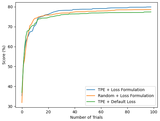
Figure 2: The best score progression measured by the average of 5 runs of models A1 to A9.

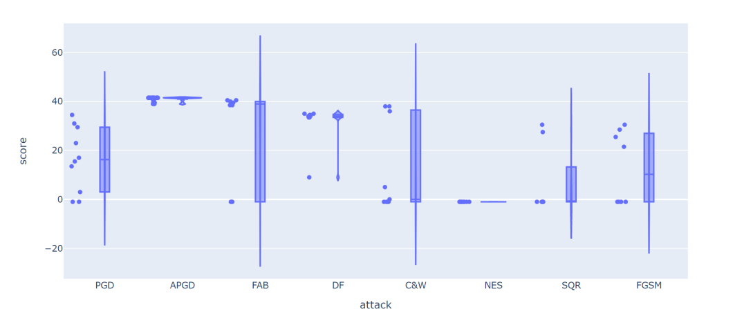
Figure 3: Attack-score distribution generated by TPE algorithm on A1 model. Scores with negative values corresponds to the time-out trials.

Appendix G Attack-Score Distribution during Search

The analysis of attack-score distribution is useful to understand A³. Figure 3 shows the distribution when running A³ on network A1. In this experiment, the number of trials is $k=100$ and the initial dataset size is $n=200$, the time budget is $T_{c}=0.5$, and we use the search space defined in Appendix B. We used single GTX1060 on this experiment. We can observe the following:

• The expensive attack times out when $T_{c}$ values are small. Here the expensive attack NES gets time-out because a small $T_{c}$ is used.

• The range and prior of attack parameters can affect the search. As we see cheap FGSM gets time-out because the search space includes large repeat parameter.

• Different attack algorithms have different parameter sensitivity. For examples, PGD has a large variance of scores, but APGD is very stable.

• TPE algorithm samples more attack algorithms with high scores. Here, there are 18 APGD trials and only 7 NES trials. TPE favours promising attack configurations so that better attack parameters can be selected during the SHA stage.

• The top attacks have similar performance, which means the searched attack should have low variance in attack strength. In practice, the variance among the best searched attacks is typically small ($\pm 0.2\%$).

Appendix H Analysis of A³ Confidence Interval

We evaluated A³ using three independent runs for models in Block A and B as reported in Table 10. The result shows typically small variation across different runs (typically less than $\pm 0.2\%$), which means A³ is consistent for robustness evaluation.

Confidence varies across different models, and the typical reason is the variance of the attacks on the same model. For examples, models A8, A9 are obfuscated and A5 is randomized, the attack has large variance due to the nature of these defenses.

Table 10: Three independent runs and confidence intervals of A³ for models in Block A and B. The bold numbers show the worst case evaluation for each model. Each confidence interval is calculated as the plus and minus the standard deviation value across the three runs. Note, that the numbers from run 3 are identical to the numbers reported in Table 1.

	Run				$\sigma$
Net	1	2	3		Confidence Interval
A1	44.79	44.7	44.69		44.73 $\pm$ 0.04
A2	2.23	2.13	1.96		2.11 $\pm$ 0.11
A3	0.10	0.10	0.11		0.10 $\pm$ 0.01
A4	3.00	3.32	3.04		3.12 $\pm$ 0.14
A5	12.73	12.74	12.14		12.54 $\pm$ 0.28
A6	4.18	4.11	3.94		4.08 $\pm$ 0.10
A7	2.73	2.71	2.71		2.72 $\pm$ 0.01
A8	10.86	10.49	11.11		10.82 $\pm$ 0.25
A9	62.62	62.31	63.56		62.83 $\pm$ 0.53
B10	62.80	62.83	62.79		62.81 $\pm$ 0.02
B11	60.43	60.04	60.01		60.16 $\pm$ 0.19
B12	59.22	59.32	59.56		59.37 $\pm$ 0.12
B13	59.54	59.54	59.51		59.53 $\pm$ 0.02
B14	57.11	57.24	57.16		57.17 $\pm$ 0.05

References

- Andriushchenko et al. (2020) Andriushchenko, M., Croce, F., Flammarion, N., and Hein, M. Square attack: A query-efficient black-box adversarial attack via random search. In Vedaldi, A., Bischof, H., Brox, T., and Frahm, J.-M. (eds.), Computer Vision – ECCV 2020, pp. 484–501, Cham, 2020. Springer International Publishing.
- Athalye et al. (2018) Athalye, A., Carlini, N., and Wagner, D. A. Obfuscated gradients give a false sense of security: Circumventing defenses to adversarial examples. In Dy, J. G. and Krause, A. (eds.), Proceedings of the 35th International Conference on Machine Learning, ICML 2018, Stockholmsmässan, Stockholm, Sweden, July 10-15, 2018, volume 80 of Proceedings of Machine Learning Research, pp. 274–283. PMLR, 2018.
- Bergstra et al. (2011) Bergstra, J., Bardenet, R., Bengio, Y., and Kégl, B. Algorithms for hyper-parameter optimization. In Shawe-Taylor, J., Zemel, R. S., Bartlett, P. L., Pereira, F. C. N., and Weinberger, K. Q. (eds.), Advances in Neural Information Processing Systems 24: 25th Annual Conference on Neural Information Processing Systems 2011. Proceedings of a meeting held 12-14 December 2011, Granada, Spain, pp. 2546–2554, 2011.
- Biggio et al. (2013) Biggio, B., Corona, I., Maiorca, D., Nelson, B., Šrndić, N., Laskov, P., Giacinto, G., and Roli, F. Evasion attacks against machine learning at test time. In Joint European conference on machine learning and knowledge discovery in databases, pp. 387–402. Springer, 2013.
- Buckman et al. (2018) Buckman, J., Roy, A., Raffel, C., and Goodfellow, I. J. Thermometer encoding: One hot way to resist adversarial examples. In 6th International Conference on Learning Representations, ICLR 2018, Vancouver, BC, Canada, April 30 - May 3, 2018, Conference Track Proceedings. OpenReview.net, 2018.
- Carlini & Wagner (2017) Carlini, N. and Wagner, D. Towards evaluating the robustness of neural networks. In 2017 IEEE Symposium on Security and Privacy (SP), pp. 39–57, 2017.
- Carlini & Wagner (2017) Carlini, N. and Wagner, D. Adversarial examples are not easily detected: Bypassing ten detection methods. In Proceedings of the 10th ACM Workshop on Artificial Intelligence and Security, AISec ’17, pp. 3–14, New York, NY, USA, 2017. Association for Computing Machinery. ISBN 9781450352024.
- Carmon et al. (2019) Carmon, Y., Raghunathan, A., Schmidt, L., Duchi, J. C., and Liang, P. S. Unlabeled data improves adversarial robustness. In Wallach, H., Larochelle, H., Beygelzimer, A., d’Alché Buc, F., Fox, E., and Garnett, R. (eds.), Advances in Neural Information Processing Systems, volume 32. Curran Associates, Inc., 2019.
- Croce & Hein (2020a) Croce, F. and Hein, M. Minimally distorted adversarial examples with a fast adaptive boundary attack. In Proceedings of the 37th International Conference on Machine Learning, ICML 2020, 13-18 July 2020, Virtual Event, volume 119 of Proceedings of Machine Learning Research, pp. 2196–2205. PMLR, 2020a.
- Croce & Hein (2020b) Croce, F. and Hein, M. Reliable evaluation of adversarial robustness with an ensemble of diverse parameter-free attacks. In Proceedings of the 37th International Conference on Machine Learning, ICML 2020, 13-18 July 2020, Virtual Event, volume 119 of Proceedings of Machine Learning Research, pp. 2206–2216. PMLR, 2020b.
- Croce et al. (2020) Croce, F., Andriushchenko, M., Sehwag, V., Flammarion, N., Chiang, M., Mittal, P., and Hein, M. Robustbench: a standardized adversarial robustness benchmark, 2020.
- Das et al. (2017) Das, N., Shanbhogue, M., Chen, S.-T., Hohman, F., Chen, L., Kounavis, M. E., and Chau, D. H. Keeping the bad guys out: Protecting and vaccinating deep learning with jpeg compression. arXiv preprint arXiv:1705.02900, 2017.
- Elsken et al. (2019) Elsken, T., Metzen, J. H., and Hutter, F. Neural architecture search: A survey, 2019.
- Falkner et al. (2018) Falkner, S., Klein, A., and Hutter, F. BOHB: robust and efficient hyperparameter optimization at scale. In Dy, J. G. and Krause, A. (eds.), Proceedings of the 35th International Conference on Machine Learning, ICML 2018, Stockholmsmässan, Stockholm, Sweden, July 10-15, 2018, volume 80 of Proceedings of Machine Learning Research, pp. 1436–1445. PMLR, 2018.
- Goodfellow et al. (2015) Goodfellow, I. J., Shlens, J., and Szegedy, C. Explaining and harnessing adversarial examples. In Bengio, Y. and LeCun, Y. (eds.), 3rd International Conference on Learning Representations, ICLR 2015, San Diego, CA, USA, May 7-9, 2015, Conference Track Proceedings, 2015.
- Gowal et al. (2021) Gowal, S., Qin, C., Uesato, J., Mann, T., and Kohli, P. Uncovering the limits of adversarial training against norm-bounded adversarial examples, 2021.
- Grathwohl et al. (2020) Grathwohl, W., Wang, K., Jacobsen, J., Duvenaud, D., Norouzi, M., and Swersky, K. Your classifier is secretly an energy based model and you should treat it like one. In 8th International Conference on Learning Representations, ICLR 2020, Addis Ababa, Ethiopia, April 26-30, 2020. OpenReview.net, 2020.
- Guo et al. (2018) Guo, C., Rana, M., Cissé, M., and van der Maaten, L. Countering adversarial images using input transformations. In 6th International Conference on Learning Representations, ICLR 2018, Vancouver, BC, Canada, April 30 - May 3, 2018, Conference Track Proceedings. OpenReview.net, 2018.
- Hu et al. (2019) Hu, S., Yu, T., Guo, C., Chao, W., and Weinberger, K. Q. A new defense against adversarial images: Turning a weakness into a strength. In Wallach, H. M., Larochelle, H., Beygelzimer, A., d’Alché-Buc, F., Fox, E. B., and Garnett, R. (eds.), Advances in Neural Information Processing Systems 32: Annual Conference on Neural Information Processing Systems 2019, NeurIPS 2019, December 8-14, 2019, Vancouver, BC, Canada, pp. 1633–1644, 2019.
- Jamieson & Talwalkar (2016) Jamieson, K. G. and Talwalkar, A. Non-stochastic best arm identification and hyperparameter optimization. In Gretton, A. and Robert, C. C. (eds.), Proceedings of the 19th International Conference on Artificial Intelligence and Statistics, AISTATS 2016, Cadiz, Spain, May 9-11, 2016, volume 51 of JMLR Workshop and Conference Proceedings, pp. 240–248. JMLR.org, 2016.
- Karnin et al. (2013) Karnin, Z. S., Koren, T., and Somekh, O. Almost optimal exploration in multi-armed bandits. In Proceedings of the 30th International Conference on Machine Learning, ICML 2013, Atlanta, GA, USA, 16-21 June 2013, volume 28 of JMLR Workshop and Conference Proceedings, pp. 1238–1246. JMLR.org, 2013.
- Lee et al. (2018) Lee, T., Edwards, B., Molloy, I., and Su, D. Defending against machine learning model stealing attacks using deceptive perturbations. arXiv preprint arXiv:1806.00054, 2018.
- Li et al. (2018) Li, L., Jamieson, K., Rostamizadeh, A., Gonina, E., Hardt, M., Recht, B., and Talwalkar, A. Massively parallel hyperparameter tuning. arXiv preprint arXiv:1810.05934, 2018.
- Liu et al. (2019) Liu, H., Simonyan, K., and Yang, Y. DARTS: differentiable architecture search. In 7th International Conference on Learning Representations, ICLR 2019, New Orleans, LA, USA, May 6-9, 2019. OpenReview.net, 2019.
- Madry et al. (2018) Madry, A., Makelov, A., Schmidt, L., Tsipras, D., and Vladu, A. Towards deep learning models resistant to adversarial attacks. In 6th International Conference on Learning Representations, ICLR 2018, Vancouver, BC, Canada, April 30 - May 3, 2018, Conference Track Proceedings. OpenReview.net, 2018.
- Mao et al. (2021) Mao, X., Chen, Y., Wang, S., Su, H., He, Y., and Xue, H. Composite adversarial attacks. Proceedings of the AAAI Conference on Artificial Intelligence, 35(10):8884–8892, May 2021. URL https://ojs.aaai.org/index.php/AAAI/article/view/17075.
- Metzen et al. (2017) Metzen, J. H., Genewein, T., Fischer, V., and Bischoff, B. On detecting adversarial perturbations. In 5th International Conference on Learning Representations, ICLR 2017, Toulon, France, April 24-26, 2017, Conference Track Proceedings. OpenReview.net, 2017.
- Moosavi-Dezfooli et al. (2016) Moosavi-Dezfooli, S., Fawzi, A., and Frossard, P. Deepfool: A simple and accurate method to fool deep neural networks. In 2016 IEEE Conference on Computer Vision and Pattern Recognition (CVPR), pp. 2574–2582, June 2016.
- Nicolae et al. (2018) Nicolae, M., Sinn, M., Minh, T. N., Rawat, A., Wistuba, M., Zantedeschi, V., Molloy, I. M., and Edwards, B. Adversarial robustness toolbox v0.2.2. CoRR, abs/1807.01069, 2018.
- Pang et al. (2019) Pang, T., Xu, K., Du, C., Chen, N., and Zhu, J. Improving adversarial robustness via promoting ensemble diversity. In Chaudhuri, K. and Salakhutdinov, R. (eds.), Proceedings of the 36th International Conference on Machine Learning, ICML 2019, 9-15 June 2019, Long Beach, California, USA, volume 97 of Proceedings of Machine Learning Research, pp. 4970–4979. PMLR, 2019.
- Papernot et al. (2015) Papernot, N., McDaniel, P. D., Wu, X., Jha, S., and Swami, A. Distillation as a defense to adversarial perturbations against deep neural networks. CoRR, abs/1511.04508, 2015.
- Paszke et al. (2019) Paszke, A., Gross, S., Massa, F., Lerer, A., Bradbury, J., Chanan, G., Killeen, T., Lin, Z., Gimelshein, N., Antiga, L., Desmaison, A., Köpf, A., Yang, E., DeVito, Z., Raison, M., Tejani, A., Chilamkurthy, S., Steiner, B., Fang, L., Bai, J., and Chintala, S. Pytorch: An imperative style, high-performance deep learning library. In Wallach, H. M., Larochelle, H., Beygelzimer, A., d’Alché-Buc, F., Fox, E. B., and Garnett, R. (eds.), Advances in Neural Information Processing Systems 32: Annual Conference on Neural Information Processing Systems 2019, NeurIPS 2019, December 8-14, 2019, Vancouver, BC, Canada, pp. 8024–8035, 2019.
- Rauber et al. (2017) Rauber, J., Brendel, W., and Bethge, M. Foolbox: A python toolbox to benchmark the robustness of machine learning models. In Reliable Machine Learning in the Wild Workshop, 34th International Conference on Machine Learning, 2017.
- Sabour et al. (2016) Sabour, S., Cao, Y., Faghri, F., and Fleet, D. J. Adversarial manipulation of deep representations. In Bengio, Y. and LeCun, Y. (eds.), 4th International Conference on Learning Representations, ICLR 2016, San Juan, Puerto Rico, May 2-4, 2016, Conference Track Proceedings, 2016.
- Sehwag et al. (2020) Sehwag, V., Wang, S., Mittal, P., and Jana, S. Hydra: Pruning adversarially robust neural networks. Advances in Neural Information Processing Systems (NeurIPS), 7, 2020.
- Stutz et al. (2020) Stutz, D., Hein, M., and Schiele, B. Confidence-calibrated adversarial training: Generalizing to unseen attacks. In Proceedings of the 37th International Conference on Machine Learning, ICML 2020, 13-18 July 2020, Virtual Event, volume 119 of Proceedings of Machine Learning Research, pp. 9155–9166. PMLR, 2020.
- Szegedy et al. (2014) Szegedy, C., Zaremba, W., Sutskever, I., Bruna, J., Erhan, D., Goodfellow, I. J., and Fergus, R. Intriguing properties of neural networks. In Bengio, Y. and LeCun, Y. (eds.), 2nd International Conference on Learning Representations, ICLR 2014, Banff, AB, Canada, April 14-16, 2014, Conference Track Proceedings, 2014.
- Tramer et al. (2020) Tramer, F., Carlini, N., Brendel, W., and Madry, A. On adaptive attacks to adversarial example defenses. arXiv preprint arXiv:2002.08347, 2020.
- Wang et al. (2019) Wang, B., Shi, Z., and Osher, S. J. Resnets ensemble via the feynman-kac formalism to improve natural and robust accuracies. In Wallach, H. M., Larochelle, H., Beygelzimer, A., d’Alché-Buc, F., Fox, E. B., and Garnett, R. (eds.), Advances in Neural Information Processing Systems 32: Annual Conference on Neural Information Processing Systems 2019, NeurIPS 2019, December 8-14, 2019, Vancouver, BC, Canada, pp. 1655–1665, 2019.
- Wierstra et al. (2008) Wierstra, D., Schaul, T., Peters, J., and Schmidhuber, J. Natural evolution strategies. In 2008 IEEE Congress on Evolutionary Computation (IEEE World Congress on Computational Intelligence), pp. 3381–3387. IEEE, 2008.
- Wu et al. (2020) Wu, D., Xia, S.-T., and Wang, Y. Adversarial weight perturbation helps robust generalization. Advances in Neural Information Processing Systems, 33, 2020.
- Xiao et al. (2020) Xiao, C., Zhong, P., and Zheng, C. Enhancing adversarial defense by k-winners-take-all. In International Conference on Learning Representations, 2020.
- Zhang & Wang (2019) Zhang, H. and Wang, J. Defense against adversarial attacks using feature scattering-based adversarial training. In Wallach, H. M., Larochelle, H., Beygelzimer, A., d’Alché-Buc, F., Fox, E. B., and Garnett, R. (eds.), Advances in Neural Information Processing Systems 32: Annual Conference on Neural Information Processing Systems 2019, NeurIPS 2019, December 8-14, 2019, Vancouver, BC, Canada, pp. 1829–1839, 2019.
- Zhang et al. (2021) Zhang, J., Zhu, J., Niu, G., Han, B., Sugiyama, M., and Kankanhalli, M. Geometry-aware instance-reweighted adversarial training. In International Conference on Learning Representations, 2021.
- Zoph & Le (2017) Zoph, B. and Le, Q. V. Neural architecture search with reinforcement learning. In 5th International Conference on Learning Representations, ICLR 2017, Toulon, France, April 24-26, 2017, Conference Track Proceedings. OpenReview.net, 2017.