STEP: Segmenting and Tracking Every Pixel

Abstract

The task of assigning semantic classes and track identities to every pixel in a video is called video panoptic segmentation. Our work is the first that targets this task in a real-world setting requiring dense interpretation in both spatial and temporal domains. As the ground-truth for this task is difficult and expensive to obtain, existing datasets are either constructed synthetically or only sparsely annotated within short video clips. To overcome this, we introduce a new benchmark encompassing two datasets, KITTI-STEP, and MOTChallenge-STEP. The datasets contain long video sequences, providing challenging examples and a test-bed for studying long-term pixel-precise segmentation and tracking under real-world conditions. We further propose a novel evaluation metric Segmentation and Tracking Quality (STQ) that fairly balances semantic and tracking aspects of this task and is more appropriate for evaluating sequences of arbitrary length. Finally, we provide several baselines to evaluate the status of existing methods on this new challenging dataset. We have made our datasets, metric, benchmark servers, and baselines publicly available, and hope this will inspire future research.

1 Introduction

Dense and pixel-precise video scene understanding is of fundamental importance for applications such as autonomous driving, film editing and spatio-temporal reasoning. More specifically, while the semantic interpretation helps with tasks such as estimating the drivable area for an autonomous vehicle, the tracking of objects enables us to anticipate the temporal evolution of the surroundings, which is critical for motion planning and obstacle avoidance.

Challenges.  Moving towards this goal, there are three challenges that we find not addressed by previous benchmarks. First, the ability of explaining every pixel of a continuous input from cameras. Second, changes in the input signal over time can happen quickly and hence, demanding that we evaluate with the same high-frequency as that of the changes that occur. Third, interpretation of continuous sensory input requires temporally consistent scene understanding, i.e., long-term tracking, which current benchmarks and metrics are not suitable for. The aim of this work is to advance this field by introducing a suitable benchmark and metric.

In the past, image benchmarks such as PASCAL VOC [21], ImageNet [52], and COCO [40] played a pivotal role in the astonishing progress of computer vision research over the last decade, allowing the community to evaluate different methods in a standardized way. Real-world datasets for various tasks [38, 57, 54, 49, 25, 13] were used to fairly measure the progress and highlight key innovations.

For the purpose of holistic image understanding, Kirillov et al. [36] introduced the concept of panoptic segmentation as a combination of semantic segmentation and instance segmentation. Kim et al. [34] subsequently introduced the notion of video panoptic segmentation (VPS). Yet, they merely label a sparse subset of pixels from short real-world video snippets that are not suitable for dense pixel-precise video understanding. Moreover, existing synthetic datasets [29, 34] struggle to evaluate performance in the real-world due to the domain shift [53].

For evaluation of VPS, existing metrics [29, 34] build upon metrics for panoptic segmentation and multi-object tracking. Since a metric can be significant in deciding the community’s research direction, biases in the metric can hinder promising innovations.

Contributions.  The contribution of this work is threefold:

(1) We introduce more suitable benchmark datasets that in particular allow spatio-temporally dense and pixel-centric evaluation. Our proposed benchmark extends the existing KITTI-MOTS, and MOTS-Challenge datasets [61] with spatially and temporally dense annotations. We seek to label every pixel with a semantic class and track ID. As in panoptic segmentation [36], we treat each non-countable region, such as the sky, as belonging to a single track. For the most salient countable classes, each instance is assigned a semantic class and a unique ID throughout the video sequences.

(2) After studying prior metrics in detail in Sec. 4, we propose the Segmentation and Tracking Quality (STQ) metric that is more suitable to access the segmentation and tracking performance of algorithms. STQ is defined at the pixel level and provides an accurate and intuitive comparison against the ground-truth at a fine-grained level. The core principle of our benchmark is that each pixel in each frame matters when evaluating an algorithm.

(3) Finally, our datasets and metric provide us a valid test-bed for evaluating several baselines that show the effect of unified vs. separate (c.f. Sec. 5) and motion- vs. appearance-based methods on our benchmark. This includes methods that use optical flow for mask propagation [47, 44, 58] or methods inspired from state-of-the-art tracking work [4, 67]. Test servers will enable a fair benchmark of methods. This provides a complete framework to enable research into dense video understanding, where both segmentation and tracking are evaluated in a detailed and holistic way. In summary,

• We present the first real-world spatially and temporally dense annotated datasets KITTI-STEP and MOTChallenge-STEP, providing challenging segmentation and (long) tracking scenes (Sec. 3).

• We analyze in-depth the recently proposed metrics [34, 29], and based on our findings propose the Segmentation and Tracking Quality (STQ) metric (Sec. 4).

• We showcase simple baselines based on established segmentation and tracking paradigms, motivating future research in end-to-end models (Sec. 5, Sec. 6).

2 Related Work

Panoptic Segmentation.  The task of panoptic segmentation combines semantic segmentation [27] and instance segmentation [24], and requires assigning a class label and instance ID to all pixels in an image. It is growing in popularity, thanks to the proposed benchmark [36]. The corresponding panoptic quality (PQ) metric is the product of recognition quality and segmentation quality.

Video Semantic Segmentation.  Compared to image semantic segmentation [21, 42, 10], video semantic segmentation [69] is less common in the literature, possibly due to the lack of benchmarks. Video semantic segmentation differs from our setting in that it does not require discriminating different instances and hence, also no explicit tracking.

Multi-Object Tracking.  The task of multi-object tracking (MOT) is to accurately track multiple objects by associating bounding boxes in videos [7, 4, 48]. Focusing on tracking, this task does not require any segmentation. The MOT-Challenge [19, 20] and KITTI-MOT [23] datasets are among the most popular benchmarks, and the tracking performance is measured by the CLEAR MOT metrics [5] along with a set of track quality measures introduced in [63]. Recently, [43] propose HOTA (Higher Order Tracking Accuracy), which explicitly balances tracking results attributed from accurate detection and association.

Video Instance Segmentation.  Combining instance segmentation and MOT, the goal of video instance segmentation (VIS) [65] is to track instance masks across video frames. This task is also known as multi-object tracking and segmentation (MOTS) [61]. Yet, the respective work adapt different evaluation metrics, focusing on different perspectives of the task. The prominent Youtube-VIS dataset [65] focuses on short sequences (3-6 seconds, every 5th frame annotated) in which objects are present from start to end. For that, ${AP}^{mask}$ [24, 40] is adapted to videos by extending the IoU to the temporal domain (3D IoU). The focus of MOTS datasets, KITTI-MOTS, and MOTS-Challenge [61], is on more general scenarios with appearing and disappearing objects within long videos. Therefore, MOTSA (Multi-Object Tracking and Segmentation Accuracy) is used, the mask-based variants of the CLEAR MOT metrics [5]. The two MOTS datasets focus on challenging urban sequences like one encounters in an autonomous driving setting. In contrast to our task, these benchmarks do not consider non-instance regions and hence, do not require pixel-precise video understanding. We build on top of these datasets by adding semantic segmentation annotations to obtain KITTI-STEP and MOTChallenge-STEP.

Video Panoptic Segmentation.  Recently, panoptic segmentation has also been extended to the video domain. Video Panoptic Segmentation (VPS) [34] requires generating the instance tracking IDs along with panoptic segmentation results across video frames. Previous datasets [34, 29] and corresponding metrics fail to properly evaluate scenarios that require both short- and long-term segmentation and tracking. Specifically, due to expensive annotation efforts for VPS datasets, most of the reported experimental results in the literature [34, 29] are conducted on synthetic datasets [50, 22], making it hard to generalize to real-world applications [28, 59]. Exceptionally, [34] annotates Cityscapes video sequences [17] for 6 frames out of each short 30 frame clip (about 1.8 seconds), hence focusing on short-term tracks. Both benchmarks [34, 29] evaluate with different metrics, VPQ (Video Panoptic Quality) and PTQ (Panoptic Tracking Quality), respectively. VPQ, tailored for sparse annotations on short clips, was not designed for evaluating long-term tracking, while PTQ penalizes recovery from association errors and may produce hard to interpret negative evaluation results. Motivated by the issues above, we propose two datasets densely annotated in space and time, KITTI-STEP and MOTChallenge-STEP requiring long-term segmentation and tracking. Additionally, we propose a novel STQ metric that gives equal importance to segmentation and tracking.

3 Datasets

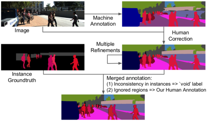
Figure 2: Annotation process: The machine annotation semantic segmentation from Panoptic-DeepLab is corrected by human annotators with multiple refinements. The resulting annotation is further merged with the existing instance ground-truth from KITTI-MOTS and MOTS-Challenge.

Overview.  We collect two densely annotated datasets in both spatial and temporal domains, i.e., every pixel in every frame is annotated, building on top of KITTI-MOTS and MOTS-Challenge [61]. Both have carefully annotated tracking IDs for ‘pedestrians’ and ‘cars’ (KITTI-MOTS only) in real-world scenes, as they are the most salient moving objects. So far, other common semantic classes in urban scenes, such as ‘bicycles’ and ‘road’, have all been grouped into one ‘background’ class, impeding pixel-level scene understanding. Therefore, our additional semantic segmentation annotation, defined by the 19 Cityscapes classes [17], enriches the KITTI-MOTS and MOTS-Challenge datasets. Specifically, all ‘background’ regions are carefully annotated, and classes that are not tracked, i.e., everything except ‘pedestrians’ and ‘cars’ in our case, are considered as a single track, similar to the ‘stuff’ definition in panoptic segmentation [36]). The resulting datasets, called KITTI-STEP and MOTChallenge-STEP, present challenging videos requiring long-term consistency in segmentation and tracking under real-world scenarios. Fig. 1 shows ground-truth annotations from the proposed dataset.

Semi-automatic annotation.  Similar to [8, 2, 61], we collect our annotations in a semi-automatic manner. In particular, we employ the state-of-the-art Panoptic-DeepLab [15, 9], pretrained on the Mapillary Vistas [46] and Cityscapes [17] datasets to generate pseudo semantic labels for each frame. The predicted semantic segmentation is then carefully refined by human annotators. On average, it takes human annotators around 10 minutes to annotate each of the more than 20000 frames. The refining process is iterated twice to guarantee high-quality per-frame annotations and consistent labels across consecutive video frames. We illustrate our semi-automatic annotation process in Fig. 2 and provide all technical details regarding the merging procedure in the supplement. It is evident from the illustration, that human refinements and corrections are required to achieve high quality annotations.

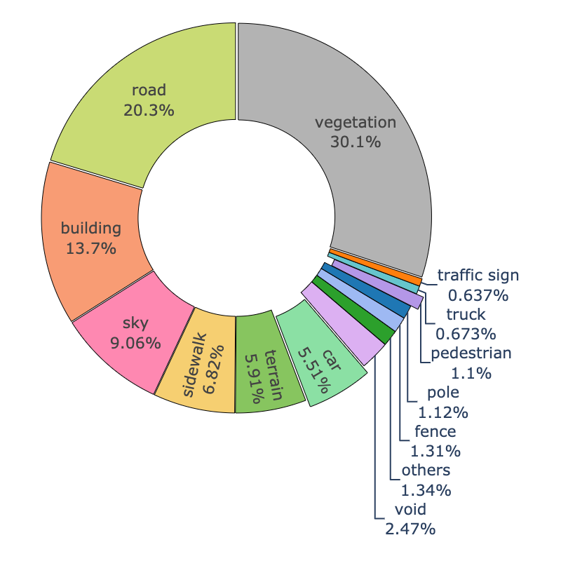
(a) KITTI-STEP.	(b) MOTChallenge-STEP.

Figure 3: Label distribution in KITTI-STEP and MOTChallenge-STEP.

KITTI-STEP dataset.  KITTI-STEP has the same train and test sequences as KITTI-MOTS (i.e., 21 and 29 sequences for training and testing, respectively). Similarly, the training sequences are further split into training set (12 sequences) and validation set (9 sequences). This dataset contains videos recorded by a camera mounted on a driving car. Since the sequence length sometimes reaches over 1000 frames, long-term tracking is required. Prior work [60] has shown that with increasing sequence length, the tracking difficulty increases too. These sequences involve regularly (re-)appearing and disappearing objects, occlusions, light condition changes and scenes of pedestrian crowds. The semantic label distribution is shown in Fig. 3.

MOTChallenge-STEP dataset.  Four sequences are annotated for MOTChallenge-STEP. In particular, we split these sequences into two for training and two for testing. This dataset contains only 7 semantic classes, as not all of Cityscapes’ 19 semantic classes are present. Even though MOTChallenge-STEP contains only one tracking class, we argue that tracking is rather difficult. First, the difficulty of tracking increases with the number of simultaneously, visually similar objects present in a scene. At the same time, this increases the chance of occlusions to occur. Concurrent work [33] has shown that this is indeed the case in the crowded MOTChallenge-STEP sequences. Second, the limited number of sequences makes training harder. We pose this as an additional challenge for future work to overcome the notion of requiring large amounts of annotated data by making use of weakly-, semi- and unsupervised approaches to improve upon our baselines. We visualize the semantic label distribution in Fig. 3.

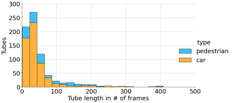
(a) Track length distributions of KITTI-STEP.

Dataset statistics	City-VPS [34]	KITTI-STEP	MOTChallenge-STEP
# Sequences (trainval/test)	450 / 50	21 / 29	2 / 2
# Frames (trainval/test)	2,700 / 300	8,008 / 11,095	1,125 / 950
# Semantic classes	19	19	7
# Annotated Masks†	72,171	126,529	17,232
Every frame annotated	✗	✓	✓
Annotated frame rate (FPS)	3.4	10	30
	Max/Mean/Min	Max/Mean/Min	Max/Mean/Min
Annotated frames per seq.†	6 / 6 / 6	1,059 / 381 / 78	600 / 562 / 525
Track length (frames)†	6 / 3 / 1	643 / 51 / 1	569 / 187 / 1

(b) Real-world dataset comparison. ^† refers to the trainval set.

Figure 4: Dataset statistics, comparison and track length distribution of KITTI-STEP.

Dataset comparison.  In Tab. 4(b), we compare KITTI-STEP and MOTChallenge-STEP with the only non-synthetic VPS dataset, Cityscapes-VPS [34]. Notably, we have more than 6 times the number of annotated frames and our longest video sequence is 176 times longer. Thus, our datasets require long-term tracking instead of focusing on short clips. KITTI-STEP contains sequences of over 1000 annotated frames that are all used to evaluate the performance. Hence, our datasets are not biased towards segmentation, as is the case when evaluating only on 6 annotated frames. Additionally, our pixel-dense annotations in space and time enable methods to work directly on video clips.

Tracking Difficulty.  As shown by [60, 33], tracking difficulty primarly increases with number of objects, occlusions and tracking length. The track length distribution in Fig. 4(a) shows the importance of long-term tracking and gives evidence that evaluating on a few frames is not representative of real-world scenarios. An extended discussing about tracking difficulty can be found in the supplement. In short, close to half of all tracks in [34] are only present in a single frame requiring no tracking. Hence, with the available annotation budget we decided to follow the best-practices in tracking benchmarks of focusing on the most salient classes as more classes does not mean harder tracking. The remaining object classes account for less than 2% of all pixels in the dataset. Therefore, our datasets present a more challenging and practical scenario, requiring both short- and long-term tracking.

Synthetic datasets.  Prior work [34] has used the synthetic dataset VIPER [50], which contains video game footage from the 2013 released game GTA5. [51] has studied the realism of VIPER. Even when showing VIPER and Cityscapes images only for 500ms, the real-world data was consistently ranked to be more realistic. Moreover, [53] has shown a large domain shift between synthetic GTA5 data and Cityscapes. Therefore, synthetic data has a purpose for pretraining, but relying purely on it does not work well enough for real-world applications, motivating the need for new benchmarks.

4 Metric

A detailed analysis of existing metrics is essential for developing a new one. We first look into basic components PQ [36] and MOTSA [61], before diving into the VPQ [34] and PTQ [29] metrics. We then condense these insights into properties that a good STEP metric should satisfy.

4.1 Metric Analysis

Panoptic Quality (PQ).  Kirillov et al. [36] proposed PQ to measure panoptic segmentation results. The set of true positive ($TP_{c}$), false positive ($FP_{c}$) and false negatives ($FN_{c}$) segments, for a particular semantic class $c$, is formed by matching predictions $p$ to ground-truth $g$ based on the IoU scores. A threshold of greater than 0.5 IoU is chosen to guarantee unique matching. The overall metric is

$$PQ_{c}=\frac{\sum_{(p,g)\in TP_{c}}IoU(p,g)}{|TP_{c}|+\frac{1}{2}|FP_{c}|+\frac{1}{2}|FN_{c}|}.$$ (1)

Defining a predicted segment with IoU of 0.51 as true positive and a segment with IoU of 0.49 as false positive (and the ground-truth segment as false negative) does not align well with human perception. Moreover, the metric is highly sensitive to false positives that cover few pixels, which is why most, if not all, panoptic segmentation methods use an additional post-processing step to remove stuff classes with few pixels or add ‘void’ class predictions [64] to increase the PQ score.

$\Rightarrow$ A metric should be insensitive to such post-processing, and consider all predictions without requiring a threshold to define true positives on a segment level.

MOTA/MOTSA.  Multi-Object Tracking Accuracy (MOTA) [5] introduced the concept of ID switches $IDSW_{c}$ between frames of the prediction w.r.t. the ground-truth $GT_{c}$. It became the standard in many tracking benchmarks [23, 45]. Its derivative Multi-Object Tracking and Segmentation Accuracy (MOTSA) [61] additionally considers segmentation, by matching objects based on segment overlap:

$$MOTSA_{c}=\frac{|TP_{c}|-|FP_{c}|-|IDSW_{c}|}{|GT_{c}|}.$$ (2)

MOTA and MOTSA were analyzed exhaustively by [43]. The most relevant drawbacks are:

1. The metric penalizes ID recovery, i.e., correcting mistakes gives worse scores.

2. The metric is unbounded and can take negative values, making scores hard to interpret.

3. The tracking precision is not considered, only recall is (c.f. [43] for details).

4. For detection, precision is much more important than recall, leading to a high imbalance.

5. Similar to PQ, MOTSA uses the threshold-based matching to define the set of true positives.

$\Rightarrow$ A metric should consider both precision and recall, and should not penalize correcting mistakes.

VPQ.  Video Panoptic Quality (VPQ) [34] for video panoptic segmentation is based on PQ and tailored to the sparsely annotated Cityscapes-VPS dataset. VPQ computes the average quality w.r.t. single frames and small spans of frames, by using a 2D and 3D IoU for matching, respectively:

$$VPQ=\frac{1}{K}\sum_{k}\frac{1}{N_{classes}}\sum_{c}\frac{\sum_{(p,g)\in TP_{c}^{k}}IoU_{2D/3D}(p,g)}{|TP_{c}^{k}|+\frac{1}{2}|FP_{c}^{k}|+\frac{1}{2}|FN_{c}^{k}|}$$ (3)

We note that these spans are constructed from every 5th video frame. Considering this averaging and that at most $K=4$ frames are taken into account, the metric puts much more emphasis on segmentation than on association. As noted in [34], when using more than 4 frames, the difficulty of the 3D IoU matching increases significantly. We agree with that assessment, but argue that we should by-pass threshold-based matching and propose a metric defined on the pixel level. When considering a setting like ours in which there are more stuff classes than countable things classes, VPQ reduces this task almost to video semantic segmentation as the metric is averaged over all classes. As a consequence, the importance of association varies with the dataset class split into stuff and things.

$\Rightarrow$ A metric should be suitable for evaluating not only short-term but also long-term tracks as well as give equal importance to segmentation and tracking, as required for real-world scenarios.

(s)PTQ.  Hurtado et al. propose the Panoptic Tracking Quality (PTQ) measure [29]:

$$PTQ_{c}=\frac{\sum_{(p,g)\in TP_{c}}IoU_{2D}(p,g)-|IDSW_{c}|}{|TP_{c}|+\frac{1}{2}|FP_{c}|+\frac{1}{2}|FN_{c}|}.$$ (4)

The metric combines PQ and MOTSA, by changing the numerator of PQ to subtract the number of ID switches $IDSW_{c}$. The metric is computed in 2D on a frame by frame basis, thus is incapable of looking beyond first-order association [43] mistakes. Also, PQ’s original threshold-based matching is applied. Following this design, PTQ inherits the drawbacks from PQ as well as most issues from MOTSA as described above.

$\Rightarrow$ A metric should evaluate videos beyond single frames and decouple segmentation and association.

Metric Requirements.  Given these insights, we argue for a change of paradigms. In detail, we define the following properties that a STEP metric should satisfy.

1. Analyze full videos at pixel level: The metric should work on full videos and at the pixel level rather than on single frames or at segment level.

2. No threshold-based matching: The metric should treat all pixels equally in space and time.

3. No penalty for mistake correction: Correcting errors in ongoing tracks should not be penalized, but encouraged to obtain long-term track consistency.

4. Consider precision and recall for association: For association errors (e.g., ID transfer), the metric should take precision and recall into account.

5. Decouple errors: The metric could be decoupled into components, enabling detailed analysis for different aspects of STEP performance.

4.2 STQ Metric

The previous discussions motivate us to propose the Segmentation and Tracking Quality (STQ).

Formal Definition.  Our benchmark requires a mapping $f$ of every pixel $(x,y,t)$ (indexed by spatial coordinates $(x,y)$ and frame $t$) of a video $\Omega$ to a semantic class $c$ and a track ID $id$. We denote the ground-truth as $gt(x,y,t)$ and the prediction as $pr(x,y,t)$. STQ combines Association Quality (AQ) and Segmentation Quality (SQ) that measure the tracking and segmentation quality, respectively.

Association Quality (AQ).  The proposed AQ is designed to work at a pixel-level of a full video (c.f., P1). Importantly, all correct and incorrect associations influence the score, independent of whether a segment is above or below an IoU threshold (c.f., P2). We define the prediction for a particular $id$ as:

$$pr_{id}(id)=\{(x,y,t)\ |\ pr(x,y,t)=(c,id),c\in\mathbf{C}^{th}\}$$ (5)

here we only consider “trackable“ objects $\mathbf{C}^{th}$, i.e., things. The ground-truth is defined analogously. Mislabeling the semantic class of a pixel is not penalized in AQ, and will only be judged by the segmentation quality described later. This decoupling prevents penalizing wrong semantic predictions twice. We also do not require a consistent semantic class label per track, for reasons illustrated in the following example: A ground-truth van track can easily be mistaken as a car, which should be penalized in the segmentation score, but not in the association score. Moreover, once it becomes clear that the predicted car is actually a van, this class prediction can be corrected which results in an overall increased score for our proposed metric. However, when requiring one semantic class per track, this prediction would be split into one track for car and one for van. As a result, this split that corrects the semantic class would receive a lower score than a prediction that keeps the wrong class, which contradicts P3. We call this effect class-recovery in line with the tracking term ID recovery.

Following the notation of [43], we define the true positive associations (TPA) of an specific ID as:

$$TPA(p,g)=|pr_{id}(p)\cap gt_{id}(g)|.$$ (6)

Similarly, false negative associations (FNA) and false positive associations (FPA) can be defined to compute precision $P_{id}$ and recall $R_{id}$ (c.f., P4). Increasing precision requires the minimization of FPAs, while increasing recall requires minimization of FNAs. We define the $IoU_{id}$ for AQ as follows:

$$IoU_{id}(p,g)=\frac{P_{id}(p,g)\times R_{id}(p,g)}{P_{id}(p,g)+R_{id}(p,g)-P_{id}(p,g)\times R_{id}(p,g)}.$$ (7)

Following our goal of long-term track consistency, we encourage ID recovery by weighting the score of each predicted tube by their TPA. Without this weighting, a recovered ID would not achieve a higher score. In total, the association quality (AQ) is defined as follows.

$$AQ=\frac{1}{|\mathrm{gt\_tracks}|}\sum_{g\in\mathrm{gt\_tracks}}\frac{1}{|gt_{id}(g)|}\sum_{p,|p\cap g|\neq\emptyset}TPA(p,g)\times IoU_{id}(p,g)$$ (8)

For each ground-truth track $g$, its association score $AQ(g)$ is normalized by its size rather than by the sum of all TPA, which penalizes the removal of correct segments with wrong IDs noticeably.

Segmentation Quality (SQ).  In semantic segmentation, Intersection-over-Union (IoU) is the most widely adopted metric [21]. As IoU only considers the semantic labels, it fulfills the property of decoupling segmentation and association (c.f., P5). Additionally, it allows us to measure the quality for crowd regions. Formally, given $pr(x,y,t)$, and class $c$ we define:

$$pr_{sem}(c)=\{(x,y,t)\ |\ pr(x,y,t)=(c,*)\},$$ (9)

The ground-truth is defined analogously. We then define SQ to be the mean IoU score:

$$SQ=mIoU=\frac{1}{|\mathbf{C}|}\sum_{c\in\mathbf{C}}\frac{|pr_{sem}(c)\cap gt_{sem}(c)|}{|pr_{sem}(c)\cup gt_{sem}(c)|},$$ (10)

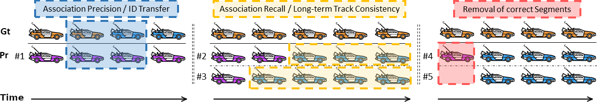
Nr.	STQ	PTQ	VPQ†
#1	0.71	1.0	0.0
#2	0.72	0.8	0.4
#3	0.82	0.8	0.53
#4	0.79	0.75	0.5
#5	0.65	0.86	0.75

Figure 5: An illustration of association precision, association recall and the removal of correct segments with wrong track ID for tracks of up to 5 frames. Each car is in a single-frame, where colors encode track IDs. We assume perfect segmentation and show matched tracks. For example, the left scenario contains two ground-truth tracks (orange , blue ), while the prediction contains a single track (violet ) that overlaps with both ground-truth tracks. Here, only the change of colors is important. Predictions should ideally have color transitions at the same frames as the ground-truth, if any. VPQ^† refers to the VPQ score when evaluated on full videos instead of small spans. STQ is the only metric that properly penalizes ID transfer (#1, P4), encourages long-term track consistency (#3 $>$ #2, P4), and reduces the score when removing semantically correct predictions (#4 $>$ #5, P5).

Segmentation and Tracking Quality (STQ).  The overall STQ score is the geometric mean:

$$STQ=(AQ\times SQ)^{\frac{1}{2}}.$$ (11)

The geometric mean is preferable over the arithmetic mean, as it rewards joint segmentation and tracking. Methods specializing in only one aspect of the task will therefore receive a lower score in this setting. The effect of association errors on all proposed metrics is illustrated in Fig. 5 with intermediate computation steps in the supplement. Tab. 1 provides a comparison of STEP metrics. We note that the computational complexity of all metrics is bound by the input size as the $IoU$ computation requires to read all pixels from all frames.

Metric Properties	STQ	PTQ [29]	VPQ [34]
P1: Analyze full videos on pixel level	✓	✗	(✓)
P2: No threshold-based matching	✓	✗	✗
P3: No penalty for mistake correction	✓	✗	✗
P4: Consider precision and recall	✓	✗	(✓)
P5: Decouple errors	✓	✗	✗

Table 1: Metric comparison. (✓): Partially satisfied. VPQ and PTQ fail to satisfy the properties.

5 Baselines

We provide single-frame and multi-frame baselines for the collected STEP datasets. Single-frame baselines follow the tracking-by-detection paradigm, i.e., obtaining predictions in each frame independently. Then we associate predicted instances over time to obtain object tracks. Thus, we use separate modules for segmentation and tracking. By contrast, the multi-frame baseline is a unified model that jointly tackles segmentation and tracking. Architectural figures are provided in the supplement.

Base network.  The state-of-art panoptic segmentation model Panoptic-DeepLab [16] is employed as the base network for both single-frame and multi-frame baselines. Panoptic-DeepLab extends DeepLab [11, 12], with an instance segmentation branch that predicts the instance center [66, 68] and regresses every pixel to its center [3, 32, 62]. We use ResNet-50 [26] as the network backbone.

Single-frame baselines.  Three different methods are used to infer the tracking IDs:

1. IoU Association. The predicted thing segments of two consecutive frames are matched, i.e., assigned the same tracking ID by Hungarian Matching [39] with a minimal mask IoU threshold $\delta=0.3$. To account for occluded objects, unmatched predictions are kept for $\sigma=10$ frames. Our method is insensitive to $\sigma$, i.e., using $\sigma=5,10,20$ yield similar results.

2. SORT Association. SORT [6] is a simple online tracking method that performs bi-partite matching between sets of track predictions and object detections based on the bounding box overlap criterion. Track predictions are obtained using the Kalman filter. Due to its simplicity, it became a standard baseline for tasks related to tracking [19, 18, 65]. In this paper, we use it as a bounding-box based instance tracking baseline using rectangles that enclose mask predictions.

3. Mask Propagation. We adopt the state-of-art optical flow method RAFT [58, 55] to warp each predicted mask at frame $t-1$ into frame $t$, followed by the IoU matching (B1). We note that RAFT is highly engineered, trained on multiple datasets and achieves outstanding performance, e.g., 50% error reduction on KITTI [23] compared to FlowNet2 [30]. We also use the forward-backward consistency check [56] to filter out occluded pixels during warping.

Multi-frame baseline.  Motivated by state-of-the-art MOT methods Tracktor [4] and CenterTrack [67], we add another prediction head, previous-offset, to the base network that regresses every pixel to its relative instance center in the previous frame. Hence, this model can predict motion directly without relying on an external network, which is only possible due to our dense annotations, i.e., such multi-frame approaches cannot be trained on sparse data as in Cityscapes-VPS. The previous predicted center heatmap and the previous frame are given as additional inputs to the network:

1. Motion-DeepLab. Using the predicted instance segmentation of the base network, the center of each instance is ‘shifted’ by the previous-offset to find the closest center (within a radius $r$) in the previous frame. We apply a greedy algorithm to match instances in decreasing order of the center’s score. Matched instances continue tracks, while unmatched centers start new tracks. Following [67], $r$ equals the geometric mean of the width and height of the predicted instance.

6 Results

We showcase the benchmark by studying the performance of different baselines on our datasets through the lens of the proposed STQ metric. In addition to our motion-guided baselines, we evaluate the performance of the state-of-the-art VPS model VPSNet [34]. It uses an optical flow network [30], trained on external densely annotated data to align feature maps from two consecutive frames. Object instances are associated using a trained appearance-based re-id model [65] among other cues.

Experimental Protocol.  We first pre-train all our baselines without their tracking functionality on Cityscapes [17], and VPSNet on Cityscapes-VPS [34]. These pre-trained networks are then fine-tuned on KITTI-STEP and MOTChallenge-STEP with their tracking functionality enabled. Detailed experimental protocol is shown in the supplement. As MOTChallenge-STEP does not have a validation set, we use sequence 9 for training and 2 for validation.

KITTI-STEP	OF	STQ	AQ	SQ	VPQ	PTQ	sPTQ	IDS	sIDS	sMOTSA	MOTSP
B1: IoU Assoc.	✗	0.58	0.47	0.71	0.44	0.48	0.48	1087	914.7	0.47	0.86
B2: SORT	✗	0.59	0.50	0.71	0.42	0.48	0.49	647	536.2	0.52	0.86
B3: Mask Propagation	✓	0.67	0.63	0.71	0.44	0.49	0.49	533	427.4	0.54	0.86
B4: Motion-DeepLab	✗	0.58	0.51	0.67	0.40	0.45	0.45	659	526.7	0.44	0.84
VPSNet [34]	✓	0.56	0.52	0.61	0.43	0.49	0.49	421	360.0	0.66	0.91

Table 2: We compare the different baselines under different metrics on the KITTI-STEP dataset. We highlight the first and second best score in each metric. OF refers to an external optical flow network.

MOTChallenge-STEP	OF	STQ	AQ	SQ	VPQ	PTQ	sPTQ	IDS	sIDS	sMOTSA	MOTSP
B1: IoU Assoc.	✗	0.42	0.25	0.69	0.55	0.59	0.59	164	107.6	0.21	0.77
B2: SORT	✗	0.36	0.19	0.69	0.54	0.58	0.58	364	254.5	0.22	0.77
B3: Mask Propagation	✓	0.41	0.25	0.69	0.55	0.58	0.59	209	139.4	0.20	0.77
B4: Motion-DeepLab	✗	0.35	0.19	0.62	0.51	0.54	0.54	326	227.5	0.28	0.81
VPSNet [34]	✓	0.24	0.17	0.34	0.25	0.28	0.28	152	146.3	0.40	0.84

Table 3: Experimental results of different baselines on the MOTChallenge-STEP dataset. We highlight the first and second best score in each metric. OF refers to an external optical flow network.

Experimental Results.  In Tab. 2, we report results of all models on KITTI-STEP. To discuss the effects of our STQ metric empirically, we also report scores obtained with VPQ [34] and PTQ [29]. As additional data points, we provide (soft) ID switches (s)IDS, sMOTSA and MOTS Precision (MOTSP) [61] scores that, in contrast to the other metrics, only evaluate ‘cars’ and ‘pedestrians’. We observe that our single-frame baselines (B1-B3) that perform panoptic segmentation and tracking separately achieve the overall highest STQ scores. When using multiple separate state-of-the-art models (one for panoptic segmentation and the one for optical flow), B3 achieves the highest performance in terms of association quality (AQ) and also overall in STQ. Both multi-frame baselines, B4 and VPSNet are tackling a significantly more challenging problem, addressing segmentation and tracking jointly within the network. This comes at the cost of a decrease in a single-task performance (c.f. SQ), which is also observed in other multi-task settings [37] such as image panoptic segmentation [36]. Initially, separate models outperformed unified models, taking significant research effort into unified models to catch up. B4 is such a unified model that does not rely on any external network and tackles panoptic segmentation and tracking jointly. When studying the effect of motion cues (B4) and appearance re-id cues (VPSNet), we notice that both significantly impact the tracking performance, as can be seen from the improvement in terms of AQ over B1.

From a tracking perspective, MOTChallenge-STEP is more challenging compared to KITTI-STEP because it contains several overlapping pedestrian tracks and a reduced amount of training data. In Tab. 3, we observe that B1 and B3 achieve a similar performance, which we attribute to the reduced inter-frame motion coming from pedestrians and the high 30 FPS frame rate. Notably, the SORT tracking fails to achieve track consistency in the scenarios of many overlapping instances. Naturally, separate segmentation and tracking models (B1-B3) are less affected by the reduced amount of training data, and therefore achieve consistently better results compared to the multi-frame baselines. However, the unified tracking and segmentation models B4 and VPSNet, need to train their tracking heads on reduced data and therefore easily run into overfitting issues as is evident from reduced scores. Specifically, VPSNet achieves a low SQ score, and therefore a low recall yet a high precision (c.f. sMOTSA, MOTSP). In contrast, B4 does better in SQ, but cannot leverage this to improve tracking.

In Tab. 2 and Tab. 3, we also show the effect of different metrics. We can experimentally confirm our findings from the metric analysis (Sec. 4). When comparing our metric STQ with VPQ and PTQ, we observe that even though tracking quality varies significantly (c.f. AQ, IDS, sMOTSA), the changes in VPQ and PTQ are rarely noticeable. This supports our theoretical findings that VPQ and PTQ evaluate this task from a segmentation perspective, leading to high scores for B1-B4 in Tab. 3, and fail to accurately reflect changes in association. This supports the need for a new perspective on this task, STEP, which equally emphasizes tracking and segmentation.

In summary, our experimental findings show that the novel STQ metric captures the essence of segmentation and tracking by considering both aspects equally. As our datasets KITTI-STEP and MOTChallenge-STEP provide dense annotations, for the first time motion and appearance cues can be leveraged in a unified model for dense, pixel-precise video scene understanding.

7 Conclusion

In this paper, we present a new perspective on the task of video panoptic segmentation. We provide a new benchmark, Segmenting and Tracking Every Pixel (STEP), to the community where we explicitly focus on measuring algorithm performance at the most detailed level possible, taking each pixel into account. For that purpose, we analyze the drawbacks of existing metrics, and propose the STQ metric. Our benchmark and metric are designed for evaluating algorithms in real-world scenarios, where understanding long-term tracking performance is important. We believe that this work provides an important STEP towards a dense, pixel-precise video understanding.

Acknowledgments.  We would like to thank Sérgio Agostinho, Deqing Sun and Siyuan Qiao for their valuable feedback, and Stefan Popov and Vittorio Ferrari for their work on the annotation tool. We would also like to thank for the supports from Google AI:D, Mobile Vision, the TUM Dynamic Vision and Learning Group, and all the Crowd Compute raters. This work has been partially funded by the German Federal Ministry of Education and Research (BMBF) under Grant No. 01IS18036B. The authors of this work take full responsibility for its content.

Appendix A Appendix

In this supplementary material, we provide

1. Benchmark checklist,

2. An extended tracking difficulty discussion (Sec. C),

3. More of our collected dataset statistics, and details about merging our semantic segmentation annotations with existing MOTS instance annotations [61] (Sec. D),

4. More discussion about metric design choices (Sec. E),

5. Network architecture details of our proposed unified STEP model, Motion-DeepLab (B4) (Sec. F),

6. More details on the experiments described in the main paper (Sec. G),

7. STQ on Cityscapes-VPS (Sec. H),

8. Video of qualitative results: https://youtu.be/NHBAvT0DXVw,

9. Code: https://github.com/google-research/deeplab2.

Appendix B Benchmark Checklist

1. https://github.com/google-research/deeplab2 includes instructions and code to reproduce our baselines.

2. http://cvlibs.net/datasets/kitti/eval_step.php includes links to the dataset, setup instructions and the test server.

3. https://motchallenge.net/data/STEP-ICCV21/ includes links to the dataset, setup instructions and the test server.

4. The proposed benchmarks are part of the 6th BMTT workshop at ICCV: https://motchallenge.net/workshops/bmtt2021/.

5. The authors of this work take full responsibility for the presented work. The maintainers and creators of the original KITTI and MOTChallenge benchmarks and the MOTS datasets did consent to this project. We respect their dataset license and release the test servers in their framework.

6. The benchmarks will be hosted on the long-standing benchmark servers of KITTI and MOTChallenge. The newly provided dataset annotations will be hosted by Google. We take responsibility for the maintenance and ensure that the datasets will be accessible.

7. We release the benchmarks with the corresponding licenses of the original datasets. The code lincense can be found at the corresponding website.

8. The dataset annotations are released as PNGs.

Appendix C Tracking Difficulty Discussion

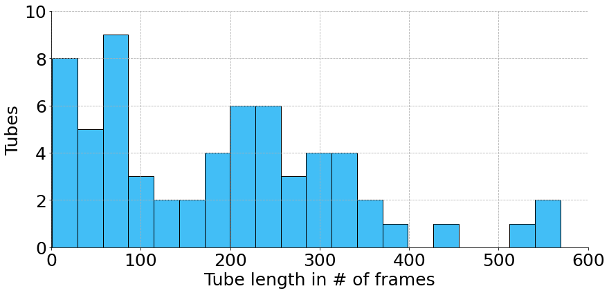
Figure 6: Track length distributions of KITTI-STEP (left) and MOTChallenge-STEP (right).

Cityscapes-VPS (val)	Person	Rider	Car	Truck	Bus	Train	Motorcycle	Bicycle	All things
Total instances	621	87	791	24	19	2	29	174	1747
Single frame instances	306	48	343	16	8	1	16	80	818
Spanning tracks	315	39	448	8	11	1	13	94	929
Average instance length	3.2	2.9	3.5	2.0	2.5	3.5	3.0	3.6	3.3

Table 4: Per-class statistics of the validation set of Cityscapes-VPS [34]. Only half of all instances need to actually be tracked, i.e., appear in more than one frame. On average, instances appear for only 3 frames showing the focus on short trajectories.

KITTI-STEP (val)	Person	Car	All things
Total instances	151	68	219
Single frame instances	0	0	0
Spanning tracks	151	68	219
Average instance length	53.2	49.2	51.9

MOTChallenge (val)	Person
Total instances	26
Single frame instances	0
Spanning tracks	26
Average instance length	183.6

Table 5: Per-class statistics of the validation set of KITTI-STEP (left) and MOTChallenge-STEP (right).

We provide a per-class breakdown of track numbers for the validation sets of Cityscapes-VPS [34] (Tab. 4), KITTI-STEP and MOTChallenge-STEP (Tab. 5). Furthermore, we show the track length distribution for both datasets in Fig. 6.

Why do only ‘pedestrians’ and ‘cars’ have tracking IDs?  In Fig. 3 in the main paper, we illustrate the class-wise histograms, i.e., amount of pixels in the whole dataset. As shown in the figure, for KITTI-STEP, both ‘cars’ and ‘pedestrians’ contain significantly more pixels compared to the rest of the classes, while for MOTChallenge-STEP, the ‘pedestrians’ dominate the others. Due to the available annotation budget we therefore decided to focus on tracking the most salient object classes ‘pedestrians’ and ‘cars’ for KITTI-STEP, and only ‘pedestrians’ for MOTChallenge-STEP. This follows the original approach by KITTI-MOTS and MOTSChallange. We note that the number of tracking classes does not causally relate to the tracking difficulty. The latter is influenced by simultaneously present objects, occlusions and sequence length. The tracking difficulty and detection difficulty are changed by different factors. As our proposed benchmarks aim to balance segmentation/detection and tracking, we focus on increasing tracking difficulty w.r.t. previous work in this area.

Long-term tracking.  In Fig. 6, we show the histograms for tracklet lengths for both datasets. As shown in the figure, our KITTI-STEP and MOTChallenge-STEP present a challenge for long term consistency in segmentation and tracking.

Do more instances or classes lead to harder tracking?  Even though, our datasets provide twice the number of masks for the trainval set compared to Cityscapes-VPS, Cityscapes-VPS provides significantly more unique instances. Here, instances refer to unique objects not distinguishing for how many frames they are visible. We refrain from calling them tracks, as tracks are usually implied to last more than a single frame. When comparing these numbers directly, Tab. 4 shows that the validation set provides 1747 unique instances, while KITTI-STEP and MOTChallenge-STEP (Tab. 5) provide only 219 and 26 instances. In the following we provide several reasons why more instances does not imply harder tracking:

1. In Cityscapes-VPS, almost half (818) of all instances (1747) only last for a single frame, hence requiring no tracking at all. This shows the strong focus of Cityscapes-VPS on the segmentation aspect.

2. The average length of instances is 3.3 on Cityscapes-VPS, i.e., instances need to be tracked for 2.3 frames after being detected. Hence, Cityscapes-VPS is not suitable to measure tracking performance. On KITTI-STEP and MOTChallenge-STEP, the average length are 51.9 and 183.6 frames, respectively.

3. The validation set of Cityscapes-VPS consists of 50 clips while our datasets contain 10 videos in the validation set. Naturally, every new clip and video always introduces a new set of instances. However, in long videos, instances continue to exist throughout (part of) the video resulting in less new instances. Yet, exactly these instances are the ones that need to be tracked and the ones that make tracking challenging.

We therefore infer that the proposed datasets KITTI-STEP and MOTChallenge-STEP are significantly more suitable when evaluating segmentation and tracking than Cityscapes-VPS. Measuring tracking requires (long) trajectories in the data.

Appendix D Extended Dataset Discussion

Merging annotation.  We merge our new semantic segmentation annotation with the existing tracking instance ground-truth, i.e., instance identity from the KITTI-MOTS and MOTS-Challenge [61]. We refer to their annotations as MOTS annotations for simplicity. Fig. 2 from the main paper gives an example of our annotation process. During the merging process, potential inconsistencies between our annotated semantic labels for the classes ‘pedestrian’ and ‘car’ and the MOTS instance annotations need to be carefully handled. For example, following the ‘pedestrian’ definition in Cityscapes [17], our semantic annotation includes items carried (but not touching the ground) by the person, while MOTS annotations exclude those items. With the aim to build a dataset that is compatible for both Cityscapes and MOTS definitions, we adopt the following strategy to merge the semantic annotations. For the cases where our annotated semantic mask is larger than MOTS annotated mask, we dilate the MOTS instance annotations with a kernel size of 15. The difference between the intersection of our annotation with the the enlarged and with the original MOTS annotations is re-labeled as ‘VOID’. In practice, the union regions are detected by dilating the MOTS instance annotations with a kernel size 15. For the cases where our annotated semantic mask is smaller than MOTS annotated mask, the inconsistent regions are overwritten with MOTS annotations. As a result, the consistent ‘pedestrian’ masks are annotated with both semantic class and tracking IDs. Small regions along the masks are annotated with ‘void’, while personal items are annotated with only the semantic class (and tracking ID 0). Additionally, the ignored regions in the MOTS annotations are filled with our semantic annotation. For the crowd regions, e.g., a group of ‘pedestrians’ that could not be distinguished by annotators, semantic labels are annotated but their tracking ID is set to 0. More technically, we denote each MOTS instance mask with semantic label l and instance ID i as $M_{l}^{i}$, and the semantic annotation mask with label k as $S_{k}$. We first dilate $M_{l}^{i}$ using a kernel with 15 pixels. There are three cases for each $S_{k}$:

Case I: $S_{k}$ intersects with $M_{l}^{i}$. The intersection is overwritten with label l with instance ID = i.

Case II: $S_{k}$ intersects with the expanded dilated region. The intersection is re-labeled as ‘void’ if $k=l$.

Case III: The semantic label of the rest without any intersection remains the same.

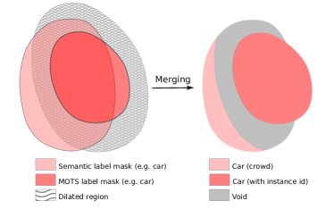
Figure 7: Illustration of how we merge the semantic and MOTS annotations. A large dilation region is chosen for illustration purpose.

This process is summarized in Fig. 7. We refer to the merged datasets as KITTI-STEP and MOTChallenge-STEP, respectively.

Appendix E Extended Metric Discussion

In addition to the overview of metrics in the main paper, we discuss one more common metric in video instance segmentation [65], and explain why it is unsuitable for STEP. After that, we will discuss our design choices of Segmentation and Tracking Quality (STQ).

E.1 Track-mAP (${AP}^{track}$)

For the task of Video Instance Segmentation [65], a variant of ${AP}^{mask}$ [24, 40] is used to measure the quality of predictions. Like ${AP}^{mask}$, ${AP}^{track}$ allows overlapping predictions, and hence requires confidence scores to rank instance proposals. These predictions are then matched with an IoU threshold. Moreover, as established in prior work [43], this metric can be gamed by making lots of low-confidence predictions, and the removal of correct detections with wrong track ID can improve scores. We therefore consider this metric unsuitable for our benchmark.

E.2 STQ Design Choices

As stated in the main paper, we define the association quality (AQ) as follows:

$$AQ(g) =\frac{1}{|gt_{id}(g)|}\sum_{p,|p\cap g|\neq\emptyset}TPA(p,g)\times IoU_{id}(p,g),$$

$$AQ =\frac{1}{|\mathrm{gt\_tracks}|}\sum_{g\in\mathrm{gt\_tracks}}AQ(g).$$ (12)

Precision and Recall.  While it is common for recognition and segmentation tasks to consider both recall and precision, this has not been widely adapted for tracking yet. For example, MOTSA does not consider precision for association. However, precision is important to penalize predicted associations that are false, i.e., false positive associations. Consider the following example: All cars in a sequences are segmented perfectly and are assigned the same track ID. As all ground-truth pixels are covered, this gives perfect recall. Yet, the overall prediction is far from being perfect by assigning the same track ID to different cars. Hence, precision is an important aspect of measuring the quality of a prediction. The other aspect to consider is recall. Considering the same example with perfect segmentation, a perfect association precision can be trivially achieved by assigning a different track ID to every pixel. As there are no false positives associations, the overall score is perfect. Yet, this does not fulfill the purpose of measuring the quality of association. Therefore, both aspects, precision and recall, have to be considered for a good metric measuring association.

IoU vs. F1.  The two most common approaches to combine precision and recall in computer vision are Intersection-over-Union, also known as the Jaccard Index, and F1, also known as the dice coefficient. IoU and F1 correlate positively and are thus both valid measures. We chose IoU for two reasons:

1. We already adopted the IoU metric for measuring segmentation. Using it for association as well leads to a more consistent formulation.

2. When comparing F1 and the IoU score, the F1 score is the harmonic mean of precision and recall and therefore closer to the average of both terms. On the other hand, IoU is somewhat closer to the minimum of precision and recall. Choosing IoU over F1 therefore emphasizes that good predictions need to consider recall and precision for association as well as highlighting innovation better.

Weighting factor TPA.  A simpler version of equation (12) would compute the average $IoU_{id}$ score without any weighting, and by normalizing with the number of partially overlapping predictions w.r.t. the ground-truth track. However, this formulation has the disadvantage that it does not consider long-term consistency of each track. Given two predicted tracks A and B, whether the IoU to the single ground-truth track are $3/5$ and $2/5$ or $4/5$ and $1/5$, both would achieve the exact same result:

$$\frac{1}{2}\times\left(\frac{3}{5}+\frac{2}{5}\right)=\frac{1}{2}\times\left(\frac{4}{5}+\frac{1}{5}\right)=\frac{1}{2}$$ (13)

As our goal is long-term consistency, we weight each $IoU_{id}$ with the $TPA$. This factor increases the importance of long-term prediction:

$$\frac{1}{5}\times\left(3\times\frac{3}{5}+2\times\frac{2}{5}\right) =\frac{13}{25}$$ (14)

$$\frac{1}{5}\times\left(4\times\frac{4}{5}+1\times\frac{1}{5}\right) =\frac{17}{25}$$ (15)

Thus, our formulation of AQ fulfills the property of getting a higher score for predictions that have overall higher long-term consistency.

Normalization by ground-truth size.  When considering the normalization factor of equation (12), one natural question that could come up is, why do we propose this denominator instead of the sum of all TPA. The reason is that otherwise the removal of correctly segmented regions with wrong track ID could achieve a higher score. Consider two predicted car tracks overlapping a ground-truth car track with IoU $4/5$ and $1/5$, respectively. Changing the denominator would lead to the following scores, with and and without the removal of the second track:

$$\frac{1}{5}\times\left(4\times\frac{4}{5}+1\times\frac{1}{5}\right) =\frac{17}{25}$$ (16)

$$\frac{1}{4}\times\left(4\times\frac{4}{5}\right) =\frac{16}{20}=\frac{20}{25}$$ (17)

Hence, the removed segment leads to a higher score. In contrast, in our current formulation we achieve the following scores in this scenario:

$$\frac{1}{5}\times\left(4\times\frac{4}{5}+1\times\frac{1}{5}\right) =\frac{17}{25}$$ (18)

$$\frac{1}{5}\times\left(4\times\frac{4}{5}\right) =\frac{16}{25}$$ (19)

Therefore, it will always be better to recognize cars (or other objects) than not to detect them. This still holds when looking at the overall metric. Even though the removal of correct segments is already penalized in the segmentation quality, that penalty would would rarely be noticeable when the association quality score would increase in that case. Hence, setting the denominator to the ground-truth size aligns with the importance of not removing predictions. For example, in an autonomous driving scenario, it is critical that correct pedestrian predictions are kept, even though they have a wrong track ID.

Class-aware vs. Class-agnostic Association.  In previous metrics, VPQ [34] and PTQ [29] tracks must have the correct semantic class assigned to count as true positives. Such design couples segmentation and association errors, e.g., a car track mistaken for a van would receive a score of 0 even though is is perfectly tracked throughout a sequence. In our setting, we compare three options to design the association score w.r.t. to semantic classes.

1. Require the correct semantic class of predicted tracks to be matched to ground-truth tracks to compute association sores.

2. Require one (but any) semantic class of predicted tracks to be matched to ground-truth tracks to compute association sores.

3. Allow any semantic thing class to be assigned to pixels of predicted tracks.

Option 1 penalizes wrong semantic segmentation twice and therefore completely couples segmentation and association errors like VPQ and PTQ. The 2nd option has the problem that correcting semantic classes receives a lower score than not correcting them. A prediction that at first mistakes a van for a car should not be penalized, when the semantic class is changed to the correct one. When requiring one semantic class, a prediction that changes the semantic class would create a new track. This would result in an overall reduced score, which violates the goal of not penalizing the correction of mistakes. Therefore, we have chosen the 3rd option for the design of our STQ metric.

Implementation Details.  We need to consider two special cases for the implementation of the STQ metric. The first case is the crowd region. For far away or highly overlapping objects, it can be impossible for human annotators to distinguish different instances. In those cases, we can still assign the correct semantic class to these pixels. During evaluation, we cannot measure any association quality, but also do not want to penalize (potentially correct) track ID assignment by a network. We therefore consider the semantic class of these regions for measuring the segmentation quality. For the association quality, these pixel regions are ignored, which means there is no penalty for assigning track IDs to these regions. The second case to consider is the ignore label. Ignore labels are commonly used by annotators for regions, which can not be assigned to one of the limited semantic classes and should therefore be ignored during evaluation. However, [36] introduced this concept for predictions, too. Predicted ignore segments do not count as false positives, which lead to common post-processing steps in the field of panoptic segmentation. Specifically, small predicted segments are overwritten with the void label. Since we would not like to encourage such tricks, we adopt the following strategy to handle void label. For the segmentation quality, we allow an additional class void, which is handled like all other classes, except that all ignore regions in the ground-truth will not be considered. Thus, there is no advantage of predicting void labels, but we still allow to evaluate output of methods that require such predictions by design.

	#1	#2	#3	#4	#5
SQ	1.0	1.0	1.0	1.0	0.75
AQ	$\frac{1}{2\times 2}(\frac{2\times 2}{4}+\frac{2\times 2}{4})=0.5$	$\frac{1}{5}(\frac{2\times 2}{5}+\frac{3\times 3}{5})=\frac{13}{25}$	$\frac{1}{5}(\frac{1\times 1}{5}+\frac{4\times 4}{5})=\frac{17}{25}$	$\frac{1}{4}(\frac{1\times 1}{4}+\frac{3\times 3}{4})=\frac{5}{8}$	$\frac{1}{4}(\frac{3\times 3}{4})=\frac{9}{16}$
STQ	$\sqrt{1\times 0.5}=0.71$	$\sqrt{1\times\frac{13}{25}}=0.72$	$\sqrt{1\times\frac{17}{25}}=0.82$	$\sqrt{1\times\frac{5}{8}}=0.79$	$\sqrt{\frac{3}{4}\times\frac{9}{16}}=0.65$
PTQ	$\frac{4-0}{4+0+0}=1.0$	$\frac{5-1}{5+0+0}=0.8$	$\frac{5-1}{5+0+0}=0.8$	$\frac{4-1}{4+0+0}=0.75$	$\frac{3-0}{3+\frac{1}{2}+0}=0.86$
VPQ†	$\frac{0}{0+\frac{1}{2}+2\times\frac{1}{2}}=0$	$\frac{0.6}{1+\frac{1}{2}+0}=0.4$	$\frac{0.8}{1+\frac{1}{2}+0}=0.53$	$\frac{0.75}{1+\frac{1}{2}+0}=0.5$	$\frac{0.75}{1+0+0}=0.75$

Table 6: Intermediate computation steps for Fig. 3 of the main paper. VPQ^† refers to the VPQ evaluation over the complete scene.

Detailed metric scores of illustration.  We provide intermediate computation steps to obtain the results of Fig. 3 of the main paper in Tab. 6.

Appendix F Network Architecture

Single-frame baselines.  Our single-frame baselines build on top of Panoptic-DeepLab [15] by additionally using three different methods to infer the tracking IDs. The adopted separate architectures are therefore the same as the original works [15, 58].

Multi-frame baseline.  Motivated by [4, 67], our multi-frame baseline, ‘Motion-DeepLab’, extends Panoptic-DeepLab [15] by adding another prediction head, Previous Center Regression, which assists in associating predicted instances between two consecutive frames. Additionally, same as CenterTrack [67], the previous predicted center heatmap and the previous image frame are given as additional inputs to the network. The network architecture is visualized in Fig. 8.

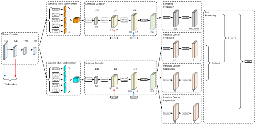
Figure 8: The architecture of the Motion-DeepLab baseline (B4).

Appendix G Experimental Results

Training Protocol.  Using Panotic-DeepLab [14] as our base network, we follow closely the same training protocol as in [14]. Specifically, all our models are trained using TensorFlow [1] on 16 TPUs and batch size 32. We use the ‘poly’ learning rate policy [41], fine-tune the batch normalization parameters [31], adopt random scale data augmentation during training with Adam [35] optimizer. Our model is pretrained on Cityscapes [17] (only image panoptic annotations are exploited) for 60k iterations with an initial learning rate of 2.5e-4. For the single-frame baselines (B1-B3), we fine-tune on KITTI-STEP and MOTChallenge-STEP with an initial learning rate of 1e-5 for 30k and 1.4k iterations, respectively. For our Motion-DeepLab baseline (B4), we have to conduct net-surgery on the weights of the first convolution of the ResNet pre-trained checkpoint [26]. The baseline B4 takes 7 channels as input (3 channels for current frame, 3 channels for previous frame, and 1 channel for the previous frame center heatmap). We therefore take the weights of the first $7\times 7$ convolution and duplicate them to get to 6 channels. Finally, the weights of the last channel are obtained by taking another duplicate and average over the channel dimension. With these pre-trained weights, we fine-tune on KITTI-STEP and MOTChallenge-STEP with a learning rate of 1e-5 for 50k and 2k iterations, respectively. For VPSNet [34], we use the default training settings to pre-train on Cityscapes-VPS without the tracking head. Then, we fine-tune the full network on KITTI-STEP and MOTChallenge-STEP again with the optimized default settings. As we observe overfitting on MOTChallenge-STEP, we reduce the training iterations to $1/3$ of the original number.

Qualitative Results.  Please refer to the attached files for video visualization of our dataset ground truth and our model predictions (B3).

Effect of pre-training.  In Tab. 7, we report the effect of pretraining our networks on Cityscapes before finetuning on KITTI-STEP. As shown in the table, pretraining brings 10%, and 4% improvement of STQ for baselines B3 and B4, respectively. For B4, we observe performance gain in SQ, and slightly degradation in AQ, presenting a challenging research problem to efficiently develop a unified STEP model. When comparing the non-pretrained networks, the unified model B4 has a much smaller gap to the B3 model than with pretraining. We hope our baseline could serve as a strong baseline to facilitate the research along the direction of developing a better unified STEP model.

Baseline	Pretrained	STQ	AQ	SQ	PQ	RQ	SQ
B3: Mask Propagation	✗	0.57	0.59	0.55	0.36	0.46	0.72
B3: Mask Propagation	✓	0.67	0.63	0.71	0.47	0.57	0.79
B4: Motion-DeepLab	✗	0.54	0.55	0.53	0.34	0.43	0.69
B4: Motion-DeepLab	✓	0.58	0.51	0.67	0.43	0.54	0.78

Table 7: Effect of pretraining on Cityscapes with results on KITTI-STEP.

Appendix H STQ on Cityscapes VPS

In Tab. 9 and Tab. 8, we show scores of our metric with VPSNet on Cityscapes-VPS. In the following, we draw insights from these numbers.

Metric insights on Cityscapes-VPS.  In Tab. 8, we provide STQ scores of VPSNet on Cityscapes-VPS. Notably, the AQ score is lower than on KITTI-STEP but higher than on MOTChallenge-STEP. In the following, we study the behavior of AQ. For that we also provide per-class scores on Cityscapes-VPS in Tab. 9.

Cityscapes-VPS (val)	STQ	AQ	SQ	VPQ	VPQTh	VPQSt
VPSNet	0.50	0.35	0.72	0.57	0.44	0.67

Table 8: VPSNet evaluated on Cityscapes-VPS [34]. Scores obtained from official code and models.

Cityscapes-VPS (val)	Person	Rider	Car	Truck	Bus	Train	Motorcycle	Bicycle	All things	All
VPQ ($K=4$)	0.32	0.35	0.45	0.32	0.34	0.43	0.27	0.28	0.34	0.52
STQ	0.51	0.48	0.63	0.46	0.38	0.31	0.26	0.44	0.50	0.50
AQ	0.30	0.30	0.42	0.29	0.20	0.18	0.18	0.27	0.35	0.35

Table 9: Per-class breakdown of thing scores of VPSNet evaluated on the validation set of Cityscapes-VPS [34]. Scores obtained from official code and models. VPQ with $K=4$ annotated frames, is the longest and hardest evaluation of VPQ under the official settings.

Due to our unified treatment of space and time, STQ can evaluate single frame performance, short clip performance as well as long video performance. Depending on the dataset, the AQ score will therefore adapt to the given characteristics. Naturally, AQ cannot measure tracking when the dataset focus is on segmentation as discussed above. Hence, AQ will measure pixel-precise image and small clip instance segmentation on Cityscapes-VPS. A lower AQ on Cityscapes-VPS does therefore not imply that tracking is harder than on KITTI-STEP. Moreover, all instances contribute equally towards the final score independent of the instance size. With almost 50% instances not being tracks, 50% of the score will be image instance segmentation.

As a reminder, VPQ is averaged over the scores when evaluating PQ on one, two, three, and four frames. In this example, AQ behaves similar as VPQK when evaluated on $K=4$ frames.

References

- [1] Martín Abadi, Paul Barham, Jianmin Chen, Zhifeng Chen, Andy Davis, Jeffrey Dean, Matthieu Devin, Sanjay Ghemawat, Geoffrey Irving, Michael Isard, et al. Tensorflow: A system for large-scale machine learning. In 12th USENIX symposium on operating systems design and implementation (OSDI 16), 2016.
- [2] Mykhaylo Andriluka, Jasper RR Uijlings, and Vittorio Ferrari. Fluid annotation: a human-machine collaboration interface for full image annotation. In Proceedings of the 26th ACM international conference on Multimedia, 2018.
- [3] Dana H Ballard. Generalizing the Hough transform to detect arbitrary shapes. Pattern Recognition, 1981.
- [4] Philipp Bergmann, Tim Meinhardt, and Laura Leal-Taixé. Tracking Without Bells and Whistles. In ICCV, 2019.
- [5] Keni Bernardin and Rainer Stiefelhagen. Evaluating Multiple Object Tracking Performance: The CLEAR MOT Metrics. JIVP, 2008.
- [6] Alex Bewley, Zongyuan Ge, Lionel Ott, Fabio Ramos, and Ben Upcroft. Simple online and realtime tracking. In ICIP, 2016.
- [7] Michael D Breitenstein, Fabian Reichlin, Bastian Leibe, Esther Koller-Meier, and Luc Van Gool. Robust tracking-by-detection using a detector confidence particle filter. In ICCV, 2009.
- [8] Lluis Castrejon, Kaustav Kundu, Raquel Urtasun, and Sanja Fidler. Annotating object instances with a polygon-rnn. In CVPR, 2017.
- [9] Liang-Chieh Chen, Raphael Gontijo Lopes, Bowen Cheng, Maxwell D. Collins, Ekin D. Cubuk, Barret Zoph, Hartwig Adam, and Jonathon Shlens. Naive-Student: Leveraging Semi-Supervised Learning in Video Sequences for Urban Scene Segmentation. In ECCV, 2020.
- [10] Liang-Chieh Chen, George Papandreou, Iasonas Kokkinos, Kevin Murphy, and Alan L Yuille. Semantic image segmentation with deep convolutional nets and fully connected CRFs. In ICLR, 2015.
- [11] Liang-Chieh Chen, George Papandreou, Iasonas Kokkinos, Kevin Murphy, and Alan L Yuille. DeepLab: Semantic image segmentation with deep convolutional nets, atrous convolution, and fully connected CRFs. TPAMI, 2017.
- [12] Liang-Chieh Chen, George Papandreou, Florian Schroff, and Hartwig Adam. Rethinking atrous convolution for semantic image segmentation. arXiv:1706.05587, 2017.
- [13] Liang-Chieh Chen, Yukun Zhu, George Papandreou, Florian Schroff, and Hartwig Adam. Encoder-decoder with atrous separable convolution for semantic image segmentation. In ECCV, 2018.
- [14] Yifeng Chen, Guangchen Lin, Songyuan Li, Omar Bourahla, Yiming Wu, Fangfang Wang, Junyi Feng, Mingliang Xu, and Xi Li. BANet: Bidirectional Aggregation Network With Occlusion Handling for Panoptic Segmentation. In CVPR, 2020.
- [15] Bowen Cheng, Maxwell D Collins, Yukun Zhu, Ting Liu, Thomas S Huang, Hartwig Adam, and Liang-Chieh Chen. Panoptic-deeplab: A simple, strong, and fast baseline for bottom-up panoptic segmentation. In CVPR, 2020.
- [16] Jingchun Cheng, Yi-Hsuan Tsai, Shengjin Wang, and Ming-Hsuan Yang. Segflow: Joint learning for video object segmentation and optical flow. In ICCV, 2017.
- [17] Marius Cordts, Mohamed Omran, Sebastian Ramos, Timo Rehfeld, Markus Enzweiler, Rodrigo Benenson, Uwe Franke, Stefan Roth, and Bernt Schiele. The Cityscapes Dataset for Semantic Urban Scene Understanding. In CVPR, 2016.
- [18] Achal Dave, Tarasha Khurana, Pavel Tokmakov, Cordelia Schmid, and Deva Ramanan. TAO: A Large-Scale Benchmark for Tracking Any Object. In ECCV, 2020.
- [19] Patrick Dendorfer, Aljoša Ošep, Anton Milan, Konrad Schindler, Daniel Cremers, Ian Reid, Stefan Roth, and Laura Leal-Taixé. MOTChallenge: A Benchmark for Single-camera Multiple Target Tracking. IJCV, 2020.
- [20] Patrick Dendorfer, Hamid Rezatofighi, Anton Milan, Javen Shi, Daniel Cremers, Ian Reid, Stefan Roth, Konrad Schindler, and Laura Leal-Taixé. MOT20: A benchmark for multi object tracking in crowded scenes. arXiv:2003.09003, 2020.
- [21] M. Everingham, L. Van Gool, C. K. I. Williams, J. Winn, and A. Zisserman. The Pascal Visual Object Classes (VOC) Challenge. IJCV, 2010.
- [22] Adrien Gaidon, Qiao Wang, Yohann Cabon, and Eleonora Vig. Virtual worlds as proxy for multi-object tracking analysis. In CVPR, 2016.
- [23] Andreas Geiger, Philip Lenz, and Raquel Urtasun. Are we ready for autonomous driving? the kitti vision benchmark suite. In CVPR, 2012.
- [24] Bharath Hariharan, Pablo Arbeláez, Ross Girshick, and Jitendra Malik. Simultaneous detection and segmentation. In ECCV, 2014.
- [25] K. He, G. Gkioxari, P. Dollár, and R. Girshick. Mask R-CNN. In ICCV, 2017.
- [26] Kaiming He, Xiangyu Zhang, Shaoqing Ren, and Jian Sun. Deep residual learning for image recognition. In CVPR, 2016.
- [27] Xuming He, Richard S Zemel, and Miguel Á Carreira-Perpiñán. Multiscale conditional random fields for image labeling. In CVPR, 2004.
- [28] Judy Hoffman, Eric Tzeng, Taesung Park, Jun-Yan Zhu, Phillip Isola, Kate Saenko, Alexei Efros, and Trevor Darrell. Cycada: Cycle-consistent adversarial domain adaptation. In ICML, 2018.
- [29] Juana Valeria Hurtado, Rohit Mohan, and Abhinav Valada. MOPT: Multi-Object Panoptic Tracking. In CVPR Workshop on Scalability in Autonomous Driving, 2020.
- [30] Eddy Ilg, Nikolaus Mayer, Tonmoy Saikia, Margret Keuper, Alexey Dosovitskiy, and Thomas Brox. Flownet 2.0: Evolution of optical flow estimation with deep networks. In CVPR, 2017.
- [31] Sergey Ioffe and Christian Szegedy. Batch normalization: accelerating deep network training by reducing internal covariate shift. In ICML, 2015.
- [32] Alex Kendall, Yarin Gal, and Roberto Cipolla. Multi-task learning using uncertainty to weigh losses for scene geometry and semantics. In CVPR, 2018.
- [33] Tarasha Khurana, Achal Dave, and Deva Ramanan. Detecting invisible people. arXiv preprint arXiv:2012.08419, 2020.
- [34] Dahun Kim, Sanghyun Woo, Joon-Young Lee, and In So Kweon. Video Panoptic Segmentation. In CVPR, 2020.
- [35] Diederik P Kingma and Jimmy Ba. Adam: a method for stochastic optimization. In ICLR, 2015.
- [36] Alexander Kirillov, Kaiming He, Ross Girshick, Carsten Rother, and Piotr Dollár. Panoptic Segmentation. In CVPR, 2019.
- [37] Iasonas Kokkinos. Ubernet: Training a universal convolutional neural network for low-, mid-, and high-level vision using diverse datasets and limited memory. In CVPR, 2017.
- [38] Alex Krizhevsky, Ilya Sutskever, and Geoffrey E Hinton. Imagenet classification with deep convolutional neural networks. In NIPS, 2012.
- [39] Harold W Kuhn. The hungarian method for the assignment problem. Naval research logistics quarterly, 2(1-2), 1955.
- [40] Tsung-Yi Lin, Michael Maire, Serge J. Belongie, Lubomir D. Bourdev, Ross B. Girshick, James Hays, Pietro Perona, Deva Ramanan, Piotr Doll’a r, and C. Lawrence Zitnick. Microsoft COCO: common objects in context. In ECCV, 2014.
- [41] Wei Liu, Andrew Rabinovich, and Alexander C Berg. Parsenet: Looking wider to see better. arXiv:1506.04579, 2015.
- [42] Jonathan Long, Evan Shelhamer, and Trevor Darrell. Fully convolutional networks for semantic segmentation. In CVPR, 2015.
- [43] Jonathon Luiten, Aljoša Ošep, Patrick Dendorfer, Philip Torr, Andreas Geiger, Laura Leal-Taixé, and Bastian Leibe. HOTA: A Higher Order Metric for Evaluating Multi-Object Tracking. IJCV, 2020.
- [44] Jonathon Luiten, Paul Voigtlaender, and Bastian Leibe. PReMVOS: Proposal-generation, Refinement and Merging for Video Object Segmentation. In ACCV, 2018.
- [45] Anton Milan, Laura Leal-Taixé, Ian Reid, Stefan Roth, and Konrad Schindler. Mot16: A benchmark for multi-object tracking. arXiv:1603.00831, 2016.
- [46] Gerhard Neuhold, Tobias Ollmann, Samuel Rota Bulo, and Peter Kontschieder. The mapillary vistas dataset for semantic understanding of street scenes. In ICCV, 2017.
- [47] Aljoša Ošep, Wolfgang Mehner, Paul Voigtlaender, and Bastian Leibe. Track, then Decide: Category-Agnostic Vision-based Multi-Object Tracking. ICRA, 2018.
- [48] Jinlong Peng, Changan Wang, Fangbin Wan, Yang Wu, Yabiao Wang, Ying Tai, Chengjie Wang, Jilin Li, Feiyue Huang, and Yanwei Fu. Chained-Tracker: Chaining Paired Attentive Regression Results for End-to-End Joint Multiple-Object Detection and Tracking. In ECCV, 2020.
- [49] Shaoqing Ren, Kaiming He, Ross Girshick, and Jian Sun. Faster r-cnn: Towards real-time object detection with region proposal networks. In C. Cortes, N. D. Lawrence, D. D. Lee, M. Sugiyama, and R. Garnett, editors, NIPS, 2015.
- [50] Stephan R Richter, Zeeshan Hayder, and Vladlen Koltun. Playing for benchmarks. In ICCV, 2017.
- [51] Stephan R. Richter, Vibhav Vineet, Stefan Roth, and Vladlen Koltun. Playing for data: Ground truth from computer games. In ECCV, 2016.
- [52] Olga Russakovsky, Jia Deng, Hao Su, Jonathan Krause, Sanjeev Satheesh, Sean Ma, Zhiheng Huang, Andrej Karpathy, Aditya Khosla, Michael Bernstein, Alexander C. Berg, and Li Fei-Fei. ImageNet Large Scale Visual Recognition Challenge. IJCV, 2015.
- [53] Swami Sankaranarayanan, Yogesh Balaji, Arpit Jain, Ser Nam Lim, and Rama Chellappa. Learning from synthetic data: Addressing domain shift for semantic segmentation. In CVPR, 2018.
- [54] Karen Simonyan and Andrew Zisserman. Very deep convolutional networks for large-scale image recognition. In ICLR, 2015.
- [55] Deqing Sun, Charles Herrmann, Varun Jampani, Mike Krainin, Forrester Cole, Austin Stone, Rico Jonschkowski, Ramin Zabih, William T. Freeman, and Ce Liu. A TensorFlow implementation of RAFT. In ECCV Robust Vision Challenge Workshop, 2020.
- [56] Narayanan Sundaram, Thomas Brox, and Kurt Keutzer. Dense point trajectories by gpu-accelerated large displacement optical flow. In ECCV, 2010.
- [57] Christian Szegedy, Wei Liu, Yangqing Jia, Pierre Sermanet, Scott Reed, Dragomir Anguelov, Dumitru Erhan, Vincent Vanhoucke, and Andrew Rabinovich. Going deeper with convolutions. In CVPR, 2015.
- [58] Zachary Teed and Jia Deng. RAFT: recurrent all-pairs field transforms for optical flow. In ECCV, 2020.
- [59] Yi-Hsuan Tsai, Wei-Chih Hung, Samuel Schulter, Kihyuk Sohn, Ming-Hsuan Yang, and Manmohan Chandraker. Learning to adapt structured output space for semantic segmentation. In CVPR, 2018.
- [60] Jack Valmadre, Luca Bertinetto, Joao F. Henriques, Ran Tao, Andrea Vedaldi, Arnold W.M. Smeulders, Philip H.S. Torr, and Efstratios Gavves. Long-term tracking in the wild: a benchmark. In ECCV, 2018.
- [61] Paul Voigtlaender, Michael Krause, Aljos̆a Os̆ep, Jonathon Luiten, Berin Balachandar Gnana Sekar, Andreas Geiger, and Bastian Leibe. MOTS: Multi-object tracking and segmentation. In CVPR, 2019.
- [62] Mark Weber, Jonathon Luiten, and Bastian Leibe. Single-shot Panoptic Segmentation. In IROS, 2020.
- [63] Bo Wu and Ram Nevatia. Tracking of multiple, partially occluded humans based on static body part detection. In CVPR, 2006.
- [64] Yuwen Xiong, Renjie Liao, Hengshuang Zhao, Rui Hu, Min Bai, Ersin Yumer, and Raquel Urtasun. UPSNet: A Unified Panoptic Segmentation Network. In CVPR, 2019.
- [65] Linjie Yang, Yuchen Fan, and Ning Xu. Video Instance Segmentation. In ICCV, 2019.
- [66] Tien-Ju Yang, Maxwell D Collins, Yukun Zhu, Jyh-Jing Hwang, Ting Liu, Xiao Zhang, Vivienne Sze, George Papandreou, and Liang-Chieh Chen. DeeperLab: Single-Shot Image Parser. arXiv:1902.05093, 2019.
- [67] Xingyi Zhou, Vladlen Koltun, and Philipp Krähenbühl. Tracking Objects as Points. In ECCV, 2020.
- [68] Xingyi Zhou, Dequan Wang, and Philipp Krähenbühl. Objects as points. arXiv:1904.07850, 2019.
- [69] Xizhou Zhu, Yuwen Xiong, Jifeng Dai, Lu Yuan, and Yichen Wei. Deep feature flow for video recognition. In CVPR, 2017.