QuPeL: Quantized Personalization with Applications to Federated Learning

Abstract

Traditionally, federated learning (FL) aims to train a single global model while collaboratively using multiple clients and a server. Two natural challenges that FL algorithms face are heterogeneity in data across clients and collaboration of clients with diverse resources. In this work, we introduce a quantized and personalized FL algorithm QuPeL that facilitates collective training with heterogeneous clients while respecting resource diversity. For personalization, we allow clients to learn compressed personalized models with different quantization parameters depending on their resources. Towards this, first we propose an algorithm for learning quantized models through a relaxed optimization problem, where quantization values are also optimized over. When each client participating in the (federated) learning process has different requirements of the quantized model (both in value and precision), we formulate a quantized personalization framework by introducing a penalty term for local client objectives against a globally trained model to encourage collaboration. We develop an alternating proximal gradient update for solving this quantized personalization problem, and we analyze its convergence properties. Numerically, we show that optimizing over the quantization levels increases the performance and we validate that QuPeL outperforms both FedAvg and local training of clients in a heterogeneous setting.

1 Introduction

Federated Learning (FL) is a learning procedure where the aim is to utilize vast amount of data residing in numerous (in millions) edge devices (clients) to train machine learning models without collecting clients’ data McMahan et al. (2017). Formally, if there are $n$ clients and $f_{i}$ denotes the local loss function at client $i$, then traditional FL learns a single global model by minimizing the following objective:

$$\operatorname*{arg\,min}_{{\bf w}\in\mathbb{R}^{d}}\Big{(}f({\bf w}):=\frac{1}{n}\sum_{i=1}^{n}f_{i}({\bf w})\Big{)}.$$ (1)

It has been realized lately that a single model cannot provide good performance to all the clients as they have heterogeneous data. This leads to the need for personalized learning, where each client wants to learn a personalized model Fallah et al. (2020); Dinh et al. (2020). Since each client may not have sufficient data to learn a good personalized model by itself, in the training process for personalized FL, clients maintain personalized models locally and utilize other clients’ data via collaborating through a global model to improve their local models. As far as we know, the personalized learning in all previous works does not respect resource diversity of clients, which is inherent to FL as the participating edge devices may vary widely in terms of resources. For instance, there might be scenarios where mobile phones, tablets, laptops all collaborate in a federated setting. In such scenarios, where edge devices are constrained to use limited resources, model compression can become critical as it would let devices with resource constraints utilize complex models.

In this work, we propose a model compression framework for personalized federated learning that addresses the both aforementioned types of heterogeneity (in data and resources) in a unified manner. Our framework lets collaboration among clients (that have different resource requirements in terms of precision of model parameters) through a full precision global model for learning quantized personalized models. Note that while training and communication are in full precision, our goal is to obtain compressed models for inference at each client. To achieve this goal in an efficient way, we learn the compression parameters for each client by including quantization levels in the optimization problem itself and carefully formulating the objective. First we investigate our approach in the centralized setup, by formulating a relaxed optimization problem and minimizing that through alternating proximal gradient steps, inspired by Bolte et al. (2014). To extend this to a distributed setup, note that performing multiple local iterations and then synchronizing the local updates with the server is usually performed in FL settings for communication efficiency Kairouz & et al. (2019). So the idea is to employ our centralized model quantization algorithm locally at clients for updating their personalized models in between synchronization indices. To aid collaboration, we introduce a term in the objective that penalizes the deviation between personalized and global models, inspired by Dinh et al. (2020); Hanzely & Richtárik (2020).

1.1 Our Contributions

Our contributions can be summarized as follows:

• To learn compressed models, we propose a novel relaxed optimization problem that enables optimization over quantization values (centers) as well as the model parameters. We use alternating proximal updates to minimize the objective and analyze its convergence properties. During training we learn both the quantization levels as well as the assignments of the model parameters to those quantization levels, while recovering the convergence rate of $\mathcal{O}(\frac{1}{T})$ in Bai et al. (2019) and Bolte et al. (2014).

• More importantly, we propose a quantized personalized federated learning scheme that allows different clients to learn models with different quantization precision and values. Besides clients’ personalized models, this provides an additional notion of personalization, namely, personalized model compression. We analyze convergence properties, and observe the common phenomenon (in personalized federated learning) that convergence rate depends on an error term related to dissimilarity of global and local gradients.

• We empirically show that optimizing over centers increases test performance and our personalization scheme outperforms FedAvg and Local Training at individual clients in a heterogeneous setting. We further observe an interesting phenomenon that clients with limited resources have increased performance when they collaborate with resource-abundant clients compared to when they collaborate with only resource-limited clients.

Our work should not be confused with works in distributed/federated learning, where models/gradients are compressed for communication efficiency Basu et al. (2019); Karimireddy et al. (2019) and not to learn compressed/quantized models for inference. On the contrary, our goal is to obtain quantized models for inference, that are suited for each client’s resources. Note that we also achieve communication efficiency, but through local iterations, not through gradient/model compression.

1.2 Related Work

To the best of our knowledge, this is the first work in personalized federated learning where the aim is to learn quantized and personalized models for inference. As a result, our work can be seen in the intersection of personalized federated learning and learning quantized models.

Personalized federated learning.

As mentioned before, personalized FL is used in heterogeneous scenarios when a single global model falls short for the learning task. Recent work adopted different approaches for learning personalized models: (i) Combine global and local models throughout the training Deng et al. (2020); Mansour et al. (2020); Hanzely & Richtárik (2020); (ii) first learn a global model and then personalize it locally by updating it using clients’ local data Fallah et al. (2020); (iii) consider multiple global models to collaborate among only those clients that share similar personalized models Zhang et al. (2021); Mansour et al. (2020); Ghosh et al. (2020); Smith et al. (2017); (iv) augment the traditional FL objective via a penalty term that enables collaboration between global and personalized models Hanzely & Richtárik (2020); Hanzely et al. (2020); Dinh et al. (2020); and (v) distillation of global model to personalized local models Lin et al. (2020).

Learning quantized models.

Training quantized neural networks has been a topic of great interest in the last few years, and extensive research resulted in training quantized networks with precision of as low as 1-bit without significant loss in performance; see Qin et al. (2020); Deng et al. (2020) for surveys. There are two main approaches in obtaining quantized models. Firstly, one can simply train a model and then do a post-training quantization that is agnostic to training procedure; see for example Banner et al. (2019). The downside of doing a post-training quantization is that the loss minimization problem for quantization is not related to the empirical loss function. Consequently, there is no guarantee that one will obtain a compressed model that has good performance. As opposed to post-training quantization, the aim of learning quantized models is to learn the quantization itself during the training Courbariaux et al. (2016, 2015). There are two kinds of approaches for training quantized networks that are of our interest. The first approximates the hard quantization function by using a soft surrogate Yang et al. (2019); Gong et al. (2019), while the other one iteratively projects the model parameters onto the fixed set of centers (Bai et al., 2019; Yin et al., 2018). Each approach has its own limitations; see Section 2 for a discussion.

While the initial focus in learning quantized networks was mainly on achieving good empirical performance, there exist some works that analyzed convergence properties. Li et al. (2017) gave the first convergence guarantees by analyzing the algorithm proposed in Courbariaux et al. (2015) using convexity assumptions. Later, Yin et al. (2018) showed convergence results for non-convex functions but under an orthogonality assumption between the quantized and unquantized weights. More recently, Bai et al. (2019) gave a convergence result for a relaxed/regularized loss function using proximal gradient updates. Note that all of the above works were done in centralized setting.

1.3 Paper Organization

In Section 2 we formulate the optimization problem to be minimized. In Sections 3 and 4, we describe our algorithms along-with the main convergence results for the centralized and personalized settings, respectively, and give the proofs in Section 5 and Section 6. Section 7 provides numerical results. Omitted proofs/details are in appendices.

2 Problem Formulation

As motivated in Section 1, in FL settings where clients with heterogeneous data also have diverse resources, our goal in this paper is for clients to collaboratively learn personalized compressed models (with potentially different precision). To this end, below, first we state our final objective function that we will end up optimizing in this paper for learning personalized compressed models, and then in the rest of this section we will argue and motivate why this particular choice of the objective is appropriate for our purpose.

Recall from (1), in the traditional FL setting, the local loss function at client $i$ is denoted by $f_{i}$. For our personalized quantized model training, we define the following augmented loss function to be minimized by client $i$:

$$F_{i}({\bf x}_{i},{\bf c}_{i},{\bf w}) :=f_{i}({\bf x}_{i})+f_{i}(\widetilde{Q}_{{\bf c}_{i}}({\bf x}_{i}))+\lambda R({\bf x}_{i},{\bf c}_{i})+\frac{\lambda_{p}}{2}\|{\bf x}_{i}-{\bf w}\|^{2}.$$ (2)

Here, ${\bf w}\in\mathbb{R}^{d}$ denotes the global model, ${\bf x}_{i}\in\mathbb{R}^{d}$ denotes the personalized model at client $i$, and ${\bf c}_{i}\in\mathbb{R}^{m_{i}}$ denotes the model quantization centers at client $i$, where $m_{i}$ is the number of centers at client $i$, with $\log m_{i}$ representing the number of bits per parameter, which could be different for each client – larger the $m_{i}$, higher the precision. Having different ${\bf c}_{i},m_{i}$’s introduces another layer of personalization, namely, personalization in the quantization itself. In (2), $\widetilde{Q}_{{\bf c}_{i}}$ denotes the soft-quantization function with respect to (w.r.t) the fixed set of centers ${\bf c}_{i}$, $R({\bf x}_{i},{\bf c}_{i})$ denotes a distance/regularizer function that encourages quantization (e.g., the $\ell_{1}$-distance, $R({\bf x},{\bf c})=\min\{\frac{1}{2}\|{\bf z}-{\bf x}\|_{1}:z_{i}\in\{c_{1},\cdots,c_{m}\},\forall i\}$ ), and $\lambda_{p}$ is the hyper-parameter controlling the regularization. We will formally define the undefined quantities later in this section. Consequently, our main objective becomes

$$\min\Big{(}F\big{(}\{{\bf x}_{i}\},\{{\bf c}_{i}\},{\bf w}\big{)}:=\frac{1}{n}\sum_{i=1}^{n}F_{i}({\bf x}_{i},{\bf c}_{i},{\bf w})\Big{)},$$ (3)

where minimization is taken over ${\bf x}_{i}\in\mathbb{R}^{d},{\bf c}_{i}\in\mathbb{R}^{m_{i}}$ for $i\in[n]$, ${\bf w}\in\mathbb{R}^{d}$, and $F_{i}({\bf x}_{i},{\bf c}_{i},{\bf w})$ for $i\in[n]$ are from (2).

In formulating (2), the last term $\frac{\lambda_{p}}{2}\|{\bf x}_{i}-{\bf w}\|^{2}$ penalizes the deviation between the personalized model ${\bf x}_{i}$ and the global model ${\bf w}$, controlled by the hyper-parameter $\lambda_{p}$. Similar augmentations have been proposed in personalized FL settings by Dinh et al. (2020) and Hanzely & Richtárik (2020), and also in a non-personalized heterogeneous setting by Li et al. Li et al. (2020). So, it suffices to motivate how we came up with the first three terms in (2), which are in fact about a centralized setting because the function $f_{i}$ and the parameters involved, i.e., ${\bf x}_{i},{\bf c}_{i}$, are local to client $i$. In the rest of this section, we will motivate this and progressively arrive at this formulation in the centralized setup. Note that as a result of minimizing the relaxed optimization problem we obtain a set of ${\bf x}_{i},{\bf c}_{i}$ for each client; obtained parameters ${\bf x}_{i}$ are concentrated around ${\bf c}_{i}^{\prime}s$ due to regularization. Consequently, ${\bf x}_{i}$ can be quantized using ${\bf c}_{i}$ without significant loss. Therefore, for inference time deployment what we do is to hard quantize ${\bf x}_{i}^{\prime}s$ using the respective ${\bf c}_{i}$.

2.1 Model Compression in the Centralized Setup

Consider a setting where an objective function $f:\mathbb{R}^{d+m}\to\mathbb{R}$ (which could be a neural network loss function) is optimized over both the quantization centers ${\bf c}\in\mathbb{R}^{m}$ and the assignment of model parameters (or weights) ${\bf x}\in\mathbb{R}^{d}$ to those centers. There are two ways to approach this problem, either by explicitly putting a constraint that weights belong to the set of centers, or embedding the quantization function into the loss function itself.

2.1.1 Two Approaches

The first approach suggests the following optimization problem: minimize $f({\bf x})$ (over ${\bf x}\in\mathbb{R}^{d},{\bf c}\in\mathbb{R}^{m}$) subject to $x_{j}\in\{c_{1},\ldots,c_{m}\}$ for all $j\in[d]$, where the constraint ensures that every component $x_{j}$ is in the set of centers. This can be equivalently written in a more succinct form as:

$$\min_{{\bf x},{\bf c}}f({\bf x})+\delta_{{\bf c}}({\bf x}),$$ (4)

where $\delta_{{\bf c}}$ denotes the indicator function, and for any ${\bf c}\in\mathbb{R}^{m},{\bf x}\in\mathbb{R}^{d}$, define $\delta_{{\bf c}}({\bf x}):=0$ if for every $j\in[d]$, $x_{j}=c$ for some $c\in\{c_{1},\ldots,c_{m}\}$, otherwise, define $\delta_{{\bf c}}({\bf x}):=\infty$.

The second approach suggests the following problem:

$$\min_{{\bf x},{\bf c}}\big{(}h({\bf x},{\bf c}):=f(Q({\bf x},{\bf c}))\big{)},$$ (5)

where $Q:\mathbb{R}^{d+m}\rightarrow\mathbb{R}^{d}$ is a quantization function that maps individual weights to the closest centers. In other words, for ${\bf x}\in\mathbb{R}^{d},{\bf c}\in\mathbb{R}^{m}$, we define $Q({\bf x},{\bf c})_{i}:=c_{k}$, where $k=\operatorname*{arg\,min}_{j\in[m]}\{|x_{i}-c_{j}|\}$. From now on, for notational convenience, we will denote $Q({\bf x},{\bf c})$ by $Q_{{\bf c}}({\bf x})$.

Limitations of both the approaches.

Both (4) and (5) have their own limitations: The discontinuity of $\delta_{{\bf c}}({\bf x})$ makes it challenging to minimize the objective function in (4). And the hard quantization function $Q_{{\bf c}}({\bf x})$ in (5) is actually a staircase function for which the derivative w.r.t. ${\bf x}$ is 0 almost everywhere, which makes it impossible to use algorithms that rely on gradients.

2.1.2 Relaxations

Inspired by some recent works that addressed the aforementioned challenges for solving (4) and (5) (without optimizing over ${\bf c}$), we propose some relaxations.

Instead of solving the optimization problem in (4) (without optimizing over ${\bf c}$), Bai et al. (2019) and Yin et al. (2018) proposed to approximate the indicator function $\delta_{{\bf c}}({\bf x})$ using a distance function $R_{\bf c}({\bf x})$, which is continuous everywhere. Note that in this case ${\bf c}$ is not an input to the function $R$ but it is a parameterization. In other words, ${\bf c}$ is not a variable that the loss function is optimized over. This suggests the following relaxation of (4):

$$\min_{{\bf x},{\bf c}}f({\bf x})+\lambda R({\bf x},{\bf c})$$ (6)

On the other hand, instead of using $Q_{\bf c}({\bf x})$ in (5) (for fixed ${\bf c}$), Yang et al. (2019) and Gong et al. (2019) proposed to use a soft quantization function $\widetilde{Q}_{\bf c}({\bf x})$ that is differentiable everywhere with derivative not necessarily 0. They used element-wise sigmoid and tanh functions, respectively. In both cases, there is a parameter $P$ that controls how closely $\widetilde{Q}_{\bf c}({\bf x})$ approximates the staircase function $Q_{\bf c}({\bf x})$. See Section 2.2 for an example of the soft quantization function. In general, as $P$ increases, $\widetilde{Q}_{\bf c}({\bf x})$ starts to become a staircase-like function, and for low $P$ (i.e., $P\rightarrow 1$), $\widetilde{Q}_{\bf c}({\bf x})$ resembles the identity function that maps $\widetilde{Q}_{\bf c}({\bf x})_{i}$ to $x_{i}$; see (Yang et al., 2019, Figure 2). Another advantage of using $\widetilde{Q}_{\bf c}({\bf x})$ instead of $Q_{\bf c}({\bf x})$ that is not exploited by previous works is that it enables the use of Lipschitz properties in the convergence analysis. This suggests the following relaxation of (5):

$$\min_{{\bf x},{\bf c}}\big{(}h({\bf x},{\bf c}):=f(\widetilde{Q}_{\bf c}({\bf x}))\big{)}.$$ (7)

Both relaxations have short-comings.

The first relaxed problem (6) does not capture how the centers should be chosen such that the neural network loss is minimized. The centers are treated as variables that should only be close to weights that are assigned to them. We believe that modeling the direct effect that centers have on the neural network loss is crucial for a complete quantized training, and we verify this through numerics; see Section 7. In the second relaxed problem (7), we can observe the effect of centers on neural network loss; however, this time the gradient w.r.t. ${\bf x}$ is heavily dependent on the choice of $\widetilde{Q}_{\bf c}$ and optimizing over ${\bf x}$ might deviate too much from optimizing the neural network loss function. For instance, when $P\rightarrow\infty$, i.e., $\widetilde{Q}_{\bf c}({\bf x})\rightarrow Q_{\bf c}({\bf x})$, gradient w.r.t. ${\bf x}$ is $0$ almost everywhere; hence, every point becomes a first order stationary point.

2.1.3 A Relaxed Problem for Model Quantization

Our aim is to come up with an objective function that would not diminish the significance of both ${\bf x}$ and ${\bf c}$ in the overall procedure. To leverage the benefits of both, we combine both optimization problems (6) and (7) into one problem:

$$\min_{{\bf x},{\bf c}}\big{(}F_{\lambda}({\bf x},{\bf c}):=f({\bf x})+\lambda R({\bf x},{\bf c})+f(\widetilde{Q}_{\bf c}({\bf x}))\big{)}.$$ (8)

Here, the first two terms help us preserve the connection of ${\bf x}$ to neural network loss function, and the last term gives us the chance of optimizing centers w.r.t. the neural network training loss itself. As a result, we have an objective function that is continuous everywhere, and for which we can use Lipschitz tools in the convergence analysis.

Remark 1.

It is important to note that with this new objective function we are able to optimize not only over weights but also over centers. This allows us to theoretically analyze how the movements of the centers affect the convergence. As far as we know, this has not been the case in the literature of quantized neural network training. Moreover, we observe numerically that optimizing over centers improves performance of the network; see Section 7.3.

2.2 An Example of the Soft Quantization Function

In this section we give an example of the soft quantization function that can be used in previous sections. In particular, we can define the following soft quantization function: $\widetilde{Q}_{\bf c}({\bf x}):\mathbb{R}^{d+m}\rightarrow\mathbb{R}^{d}$ and $\widetilde{Q}_{\bf c}({\bf x})_{i}:=\sum_{j=2}^{m}(c_{j}-c_{j-1})\sigma(P(x_{i}-\frac{c_{j}+c_{j-1}}{2}))+c_{1}$ where $\sigma$ denotes the sigmoid function and $P$ is a parameter controlling how closely $\widetilde{Q}_{\bf c}({\bf x})$ approximates $Q_{\bf c}({\bf x})$. Note that as $P\rightarrow\infty$, $\widetilde{Q}_{\bf c}({\bf x})\rightarrow Q_{\bf c}({\bf x})$. This function can be seen as a simplification of the function that was used in Yang et al. (2019).

Assumption. For all $j\in[m]$, $c_{j}$ is in a compact set. In other words, there exists a finite $c_{\max}$ such that $|c_{j}|\leq c_{\max}$ for all $j\in[m]$.

In addition, we assume that the centers are sorted, i.e., $c_{1}<\cdots<c_{m}$. Now, we state several useful facts.

Fact 1.

$\widetilde{Q}_{\bf c}({\bf x})$ is continuously and infinitely differentiable everywhere.

Fact 2.

$\sigma({\bf x})$ is a Lipschitz continuous function.

Fact 3.

Sum of Lipschitz continuous functions is also Lipschitz continuous.

Fact 4.

Product of bounded and Lipschitz continuous functions is also Lipschitz continuous.

Fact 5.

Let $g:\mathbb{R}^{n}\rightarrow\mathbb{R}^{m}$. Then, the coordinate-wise Lipschitz continuity implies overall Lipschitz continuity. In other words, let $g_{i}$ be the i’th output then if $g_{i}$ is Lipschitz continuous for all $i$, then $g$ is also Lipschitz continuous.

In our convergence analysis, we will require that $\widetilde{Q}_{\bf c}({\bf x})$ is Lipschitz continuous as well as smooth with respect to both ${\bf x}$ and ${\bf c}$. We show these properties in the following claims which we prove in Appendix A.4.

Claim 1.

$\widetilde{Q}_{\bf c}({\bf x})$ is $l_{Q_{1}}$-Lipschitz continuous and $L_{Q_{1}}$-smooth with respect to ${\bf x}$.

Claim 2.

$\widetilde{Q}_{\bf c}({\bf x})$ is $l_{Q_{2}}$-Lipschitz continuous and $L_{Q_{2}}$-smooth with respect to ${\bf c}$.

The example we gave in this section is simple yet provides technical necessities we require in the analysis. Other examples can also be used as long as they provide the smoothness properties that we utilize in the next sections.

3 Centralized Model Quantization Training

The goal of this section is to learn a quantized model for inference which can be deployed in a memory-constrained setting where storing a full precision model is not feasible. For this, we propose a training scheme (described in Algorithm 1) for minimizing (8) by optimizing over ${\bf x}\in\mathbb{R}^{d}$ (the model parameters) and ${\bf c}\in\mathbb{R}^{m}$ (quantization values/centers). Note that we keep ${\bf x}$ full precision during training and learn the optimal quantization parameters ${\bf c}$ through Algorithm 1. The learned quantization values are then used to hard-quantize the personalized models to get compressed models for deployment, as noted in Section 2.

Before we begin with the description of our algorithm we define the proximal mapping. Let $g:\mathbb{R}^{n}\rightarrow\mathbb{R}$. Given ${\bf x}\in\mathbb{R}^{n}$ and $t>0$, the proximal map of $g$ is defined as:

$$\text{prox}_{tg}({\bf x}):={\operatorname*{arg\,min}_{{\bf u}\in\mathbb{R}^{n}}}\left\{tg({\bf u})+\frac{1}{2}\|{\bf u}-{\bf x}\|^{2}\right\}={\operatorname*{arg\,min}_{{\bf u}\in\mathbb{R}^{n}}}\left\{g({\bf u})+\frac{1}{2t}\|{\bf u}-{\bf x}\|^{2}\right\}$$ (9)

Particularly, if $g({\bf x})=\delta_{A}({\bf x})$ is the indicator function of $A$, the proximal map reduces to the projection:

$$\text{prox}_{tg}({\bf x})=\text{proj}_{A}({\bf x})=\operatorname*{arg\,min}_{{\bf u}\in A}\|{\bf u}-{\bf x}\|^{2}$$ (10)

In our algorithm $g$ will correspond to $\lambda R({\bf x},{\bf c})$. Note that as $\lambda\rightarrow\infty$ we have $\lambda R({\bf x},{\bf c})\rightarrow\delta_{\mathcal{C}}({\bf x})$. As a result, $\text{prox}_{\eta\lambda R}$ can be seen as a soft projection.

As a shorthand notation, for centralized case, we will use $\text{prox}_{\eta_{1}\lambda R_{{\bf c}^{t}}}$ to denote $\text{prox}_{\eta_{1}\lambda R(\cdot,{\bf c}^{t})}$, and $\text{prox}_{\eta_{2}\lambda R_{{\bf x}^{t+1}}}$ to denote $\text{prox}_{\eta_{2}\lambda R({\bf x}^{t+1},\cdot)}$. Similarly for the personalized case, we will use $\text{prox}_{\eta_{1}\lambda R_{{\bf c}^{t}_{i}}}$ to denote $\text{prox}_{\eta_{1}\lambda R(\cdot,{\bf c}^{t}_{i})}$, and $\text{prox}_{\eta_{2}\lambda R_{{\bf x}^{t+1}_{i}}}$ to denote $\text{prox}_{\eta_{2}\lambda R({\bf x}^{t+1}_{i},\cdot)}$.

Algorithm 1 Centralized Model Quantization Scheme

Input: Regularization parameter $\lambda$; initialize the full precision model ${\bf x}^{0}$ and quantization centers ${\bf c}^{0}$; a penalty function enforcing quantization $R({\bf x},{\bf c})$; a soft quantizer $\widetilde{Q}_{{\bf c}}({\bf x})$; and learning rates $\eta_{1},\eta_{2}$.

1:  for $t=0$ to $T-1$ do

2:     Compute ${\bf g}^{t}:=\nabla_{{\bf x}^{t}}f({\bf x}^{t})+\nabla_{{\bf x}^{t}}f(\widetilde{Q}_{{\bf c}^{t}}({\bf x}^{t}))$

3:     ${\bf x}^{t+1}=\text{prox}_{\eta_{1}\lambda R_{{\bf c}^{t}}}({\bf x}^{t}-\eta_{1}{\bf g}^{t})$

4:     Compute ${\bf h}^{t}=\nabla_{{\bf c}^{t}}f(\widetilde{Q}_{{\bf c}^{t}}({\bf x}^{t+1}))$

5:     ${\bf c}^{t+1}=\text{prox}_{\eta_{2}\lambda R_{{\bf x}^{t+1}}}({\bf c}^{t}-\eta_{2}{\bf h}^{t})$

6:  end for

Output: Quantized model $\hat{{\bf x}}^{T}=Q_{{\bf c}^{T}}({\bf x}^{T})$, i.e., for $i\in[d]$, map $x^{T}_{i}$ to the nearest $c^{T}_{j}$, the $j$’th component of ${\bf c}^{T}$.

3.1 Description of the Algorithm

We optimize (8) through alternating proximal gradient descent steps. The model parameters and the quantization vector are initialized to random vectors ${\bf x}^{0}$ and ${\bf c}^{0}$, respectively. We have two learning rates $\eta_{1},\eta_{2}$ for updating ${\bf x}^{t},{\bf c}^{t}$, respectively. Note that the objective in (8) is composed of two parts: the loss function $f({\bf x})+f(\tilde{Q}_{{\bf c}}({\bf x}))$ and a quantization inducing term $R({\bf x},{\bf c})$, which we control by a regularization coefficient $\lambda$. At each iteration $t$, we first compute the gradient ${\bf g}^{t}$ of the loss function w.r.t. ${\bf x}^{t}$ (line 2), and then take the gradient step followed by the $\mathrm{prox}$ step for updating ${\bf x}^{t}$ to ${\bf x}^{t+1}$ (line 3). For the centers, first we compute the gradient ${\bf h}^{t}$ of the loss function w.r.t. ${\bf c}^{t}$ (line 4), and then take the gradient step followed by the $\mathrm{prox}$ step for updating ${\bf c}^{t}$ to ${\bf c}^{t+1}$ (line 5). Thus both the update steps ensure that we simultaneously learn model parameter and quantization vector tied together through proximal mapping of the regularization function $R$. Finally, to obtain the compressed model for deployment, in line 7 we quantize the full-precision model ${\bf x}^{T}$ with the set of centers ${\bf c}^{T}$ using $Q_{{\bf c}^{T}}$, which maps components of ${\bf x}^{T}$ to the nearest component of ${\bf c}^{T}$, as explained after (5). In Algorithm 1, we consider gradient descent as the update rule in computations of ${\bf g}^{t}$ and ${\bf h}^{t}$; however, one can also employ other methods such as SGD and ADAM.

3.2 Convergence Result

We now provide convergence guarantee for Algorithm 1 for general smooth objectives. We first state the assumptions required for deriving our results.

A.1 (Finite lower bound of $f$): We assume that $f({\bf x})>-\infty$ for all ${\bf x}\in\mathbb{R}^{d}$, which implies that $F_{\lambda}({\bf x},{\bf c})>-\infty$ for any ${\bf x}\in\mathbb{R}^{d},{\bf c}\in\mathbb{R}^{m},\lambda\in\mathbb{R}$.

A.2 (Smoothness of $f$): $f$ is $L$-smooth, i.e., for all ${\bf x},{\bf y}\in\mathbb{R}^{d}$, we have $f({\bf y})\leq f({\bf x})+\left\langle\nabla f({\bf x}),{\bf y}-{\bf x}\right\rangle+\frac{L}{2}\|{\bf x}-{\bf y}\|^{2}$.

A.3 (Bounded gradients of $f$): There exists a finite constant $G<\infty$ such that $\|\nabla f({\bf x})\|_{2}\leq G$ holds for all ${\bf x}\in\mathbb{R}^{d}$.

A.4 (Smoothness of the soft quantizer): We assume that $\widetilde{Q}_{{\bf c}}({\bf x})$ is $l_{Q_{1}}$-Lipschitz and $L_{Q_{1}}$-smooth w.r.t. ${\bf x}$, i.e., for any ${\bf c}\in\mathbb{R}^{m}$, the following holds for all ${\bf x},{\bf y}\in\mathbb{R}^{d}$:

$$\|\widetilde{Q}_{{\bf c}}({\bf x})-\widetilde{Q}_{{\bf c}}({\bf y})\| \leq l_{Q_{1}}\|{\bf x}-{\bf y}\|\$$

$$\|\nabla_{{\bf x}}\widetilde{Q}_{{\bf c}}({\bf x})-\nabla_{{\bf y}}\widetilde{Q}_{{\bf c}}({\bf y})\| \leq L_{Q_{1}}\|{\bf x}-{\bf y}\|\$$

And that $\widetilde{Q}_{{\bf c}}({\bf x})$ is $l_{Q_{2}}$-Lipschitz and $L_{Q_{2}}$-smooth w.r.t. ${\bf c}$, i.e., for any ${\bf x}\in\mathbb{R}^{d}$, the following holds for all ${\bf c},{\bf d}\in\mathbb{R}^{m}$:

$$\|\widetilde{Q}_{{\bf c}}({\bf x})-\widetilde{Q}_{{\bf d}}({\bf x})\| \leq l_{Q_{2}}\|{\bf c}-{\bf d}\|\$$

$$\|\nabla_{{\bf c}}\widetilde{Q}_{{\bf c}}({\bf x})-\nabla_{{\bf d}}\widetilde{Q}_{{\bf d}}({\bf x})\| \leq L_{Q_{2}}\|{\bf c}-{\bf d}\|\$$

A.5 (Bound on partial gradients of the soft quantizer): There exists constants $G_{Q_{1}},G_{Q_{2}}<\infty$ such that:

$$\|\nabla_{{\bf x}}\widetilde{Q}_{{\bf c}}({\bf x})\|_{F} =\|\nabla\widetilde{Q}_{{\bf c}}({\bf x})_{1:d,:}\|_{F}\leq G_{Q_{1}}$$

$$\|\nabla_{{\bf c}}\widetilde{Q}_{{\bf c}}({\bf x})\|_{F} =\|\nabla\widetilde{Q}_{{\bf c}}({\bf x})_{d+1:d+m,:}\|_{F}\leq G_{Q_{2}}$$

where ${\bf X}_{p:q,:}$ denotes the sub-matrix of ${\bf X}$ containing rows between $p$ and $q$, and $\|\cdot\|_{F}$ is the Frobenius norm.

Now we state our main convergence result of Algorithm 1 for minimizing $F_{\lambda}({\bf x},{\bf c})$ in (8) w.r.t. $({\bf x},{\bf c})\in\mathbb{R}^{d+m}$. In the following theorem we provide the first-order guarantees for convergence of $({\bf x},{\bf c})$ to a stationary point.

Theorem 1.

Consider running Algorithm 1 for $T$ iterations with $\eta_{1}=\nicefrac{{1}}{{2(L+GL_{Q_{1}}+G_{Q_{1}}Ll_{Q_{1}})}}$ and $\eta_{2}=\nicefrac{{1}}{{2(GL_{Q_{2}}+G_{Q_{2}}Ll_{Q_{2}})}}$. For any $t\in[T]$, define ${\bf G}^{t}:=[\nabla_{{\bf x}^{t+1}}F_{\lambda}\left({\bf x}^{t+1},{\bf c}^{t}\right)^{T},\nabla_{{\bf c}^{t+1}}F_{\lambda}\left({\bf x}^{t+1},{\bf c}^{t+1}\right)^{T}]^{T}$. Then, under assumptions A.1-A.5, we have:

$$\frac{1}{T}\sum_{t=0}^{T-1}\|{\bf G}^{t}\|^{2}_{2} =\mathcal{O}\left(\frac{L_{\max}^{2}\left(F_{\lambda}\left({\bf x}^{0},{\bf c}^{0}\right){-}F_{\lambda}({\bf x}^{T},{\bf c}^{T})\right)}{L_{\min}T}\right),$$

where $L_{\min}=\min\{L+GL_{Q_{1}}+G_{Q_{1}}Ll_{Q_{1}},GL_{Q_{2}}+G_{Q_{2}}Ll_{Q_{2}}\}$ and $L_{\max}=\max\{L+GL_{Q_{1}}+G_{Q_{1}}Ll_{Q_{1}},GL_{Q_{2}}+G_{Q_{2}}Ll_{Q_{2}})\}$.

We prove Theorem 1 in Section 5. Note that we recover $\frac{1}{T}$ convergence rate in Bolte et al. (2014); Bai et al. (2019).

4 QuPeL: Personalized Quantization for FL

In this section, we extend Algorithm 1 to the distributed/federated setting for learning quantized and personalized models for each client. As mentioned in Section 1, we do so by performing multiple local iterations at clients and use our centralized scheme locally at clients for updating their local models before synchronizing with the server. To this end, we propose a new algorithm QuPeL (described in Algorithm 2) for optimizing (3) over $\left(\{{\bf x}_{i},{\bf c}_{i}\}_{i=1}^{n},{\bf w}\right)$, where ${\bf x}_{i},{\bf c}_{i}$ respectively denote the model parameters and the quantization vector (centers) for client $i$, and ${\bf w}$ denotes the global model that facilitates collaboration among clients, which is encouraged through a penalty term in the local objectives (2). As discussed in Section 2, ${\bf c}_{1},\ldots,{\bf c}_{n}$ could be different in length, which allows QuPeL to learn models with different precision for different clients based on their memory constraints. Thus, QuPeL simultaneously addresses two important personalization aspects, one for heterogeneous data and the other for resource diversity.

Algorithm 2 QuPeL: Quantized Personalization Learning

Input: Regularization parameters $\lambda,\lambda_{p}$; synchronization gap $\tau$; for each client $i\in[n]$, initialize full precision personalized model ${\bf x}_{i}^{0}$, quantization centers ${\bf c}_{i}^{0}$, and local model ${\bf w}_{i}^{0}$; a penalty function enforcing quantization $R({\bf x},{\bf c})$; a soft quantizer $\widetilde{Q}_{{\bf c}}({\bf x})$; and learning rates $\eta_{1},\eta_{2},\eta_{3}$.

1:  for $t=0$ to $T-1$ do

2:     On Clients $i=1$ to $n$ (in parallel) do:

3:     if $\tau$ does not divide $t$ then

4:        Compute ${\bf g}_{i}^{t}:=\nabla_{{\bf x}_{i}^{t}}f_{i}({\bf x}_{i}^{t})+\nabla_{{\bf x}_{i}^{t}}f_{i}(\widetilde{Q}_{{\bf c}_{i}^{t}}({\bf x}_{i}^{t}))$

5:        ${\bf x}_{i}^{t+1}=\text{prox}_{\eta_{1}\lambda R_{{\bf c}_{i}^{t}}}({\bf x}_{i}^{t}-\eta_{1}({\bf g}_{i}^{t}+\lambda_{p}({\bf x}_{i}^{t}-{\bf w}_{i}^{t})))$

6:        Compute ${\bf h}_{i}^{t}:=\nabla_{{\bf c}_{i}^{t}}f_{i}(\widetilde{Q}_{{\bf c}_{i}^{t}}({\bf x}_{i}^{t+1}))$

7:        ${\bf c}_{i}^{t+1}=\text{prox}_{\eta_{2}\lambda R_{{\bf x}_{i}^{t+1}}}({\bf c}_{i}^{t}-\eta_{2}{\bf h}_{i}^{t})$

8:        ${\bf w}_{i}^{t+1}={\bf w}_{i}^{t}-\eta_{3}\lambda_{p}({\bf x}_{i}^{t+1}-{\bf w}_{i}^{t})$

9:     else

10:        Send ${\bf w}_{i}^{t}$ to Server

11:        Receive ${\bf w}^{t}$ from Server and set ${\bf w}_{i}^{t+1}={\bf w}^{t}$

12:     end if

13:     On Server do:

14:     if $\tau$ divides $t$ then

15:        Receive $\{{\bf w}_{i}^{t}\}_{i=1}^{n}$ and compute ${\bf w}^{t}:=\frac{1}{n}\sum_{i=1}^{n}{\bf w}_{i}^{t}$

16:        Broadcast ${\bf w}^{t}$ to all Clients

17:     end if

18:  end for

19:  $\hat{{\bf x}}_{i}^{T}=Q_{{\bf c}_{i}^{T}}({\bf x}_{i}^{T})$ for all $i\in[n]$

Output: Quantized personalized models $\hat{{\bf x}}_{i}^{T}$ for $i\in[n]$

4.1 Description of the Algorithm

Since clients perform local iterations, apart from maintaining ${\bf x}_{i}^{t},{\bf c}_{i}^{t}$ at client $i\in[n]$, it also maintains a model ${\bf w}_{i}^{t}$ which helps in utilizing other clients’ data via collaboration. We call set $\{{\bf w}_{i}^{t}\}$ local copies of the global model at clients at time $t$; client $i$ updates ${\bf w}_{i}^{t}$ in between communication rounds based on its local data and synchronizes that with the server who aggregates all of them to update the global model. Note that the local objective for each node $i\in[n]$ in (2) can be split into two terms: the loss function $f_{i}({\bf x}_{i})+f_{i}(\widetilde{Q}_{{\bf c}_{i}}({\bf x}_{i}))+\frac{\lambda_{p}}{2}\|{\bf x}_{i}-{\bf w}_{i}\|^{2}$ and the term enforcing quantization $\lambda R({\bf x}_{i},{\bf c}_{i})$. At any step $t$ that is not a communication round (line 3), client $i$ first computes the gradient ${\bf g}_{i}^{t}$ of the loss function w.r.t. ${\bf x}_{i}^{t}$ (line 4) and then takes a gradient step followed by the proximal step using $R$ (line 5) to update from ${\bf x}_{i}^{t}$ to ${\bf x}_{i}^{t+1}$. Then it computes the gradient ${\bf h}_{i}^{t}$ of the loss function w.r.t. ${\bf c}_{i}^{t}$ (line 6) and takes the update step for the centers followed by the proximal step (line 7). Finally, it updates ${\bf w}_{i}^{t}$ to ${\bf w}_{i}^{t+1}$ by taking a gradient step of the loss function at ${\bf w}_{i}^{t}$ (line 8). Note that, unlike in the centralized case, in QuPeL, the local training of ${\bf x}_{i}^{t},{\bf c}_{i}^{t}$ also incorporates knowledge from other clients’ data through ${\bf w}_{i}^{t}$. In a communication round (when $t$ is divisible by $\tau$), clients upload $\{{\bf w}_{i}^{t}\}$ to the server (line 10) which aggregates them (line 15) and broadcasts the updated global model to all clients (line 16). At the end of training, clients learn their personalized models $\{{\bf x}_{i}^{T}\}_{i=1}^{n}$ and quantization centers $\{{\bf c}_{i}^{T}\}_{i=1}^{n}$. Client $i$ then quantizes ${\bf x}_{i}^{T}$ to the values in ${\bf c}_{i}^{T}$ using $Q_{{\bf c}_{i}^{T}}$ (line 19), as we did in Algorithm 1.

4.2 Convergence Result

We now discuss the convergence rate for QuPeL for general smooth objectives. In addition to the assumptions A.1-A.5 made in Section 3 (for each client) we need one more assumption that bounds heterogeneity in the local datasets across all clients.

A.6 (Bounded diversity): At any $t\in\{0,\cdots,T-1\}$ and any client $i\in[n]$, the variance of the local gradient (at client $i$) w.r.t. the global gradient is bounded, i.e., there exists $\kappa_{i}<\infty$, such that for every $\{{\bf x}_{i}^{t+1}\in\mathbb{R}^{d},{\bf c}_{i}^{t+1}\in\mathbb{R}^{m_{i}}:i\in[n]\}$ and ${\bf w}^{t}\in\mathbb{R}^{d}$ generated according to Algorithm 2, we have:

$$\Big{\|}\nabla_{{\bf w}^{t}}F_{i}({\bf x}_{i}^{t+1},{\bf c}_{i}^{t+1},{\bf w}^{t})-\frac{1}{n}\sum_{j=1}^{n}\nabla_{{\bf w}^{t}}F_{j}({\bf x}_{j}^{t+1},{\bf c}_{j}^{t+1},{\bf w}^{t})\Big{\|}^{2}\leq\kappa_{i},$$

This assumption is a variant of the bounded diversity assumption in Dinh et al. (2020); Fallah et al. (2020); the variance is due to the formulation of our objective function. In particular, diversity assumption (Assumption 5) in Fallah et al. (2020) is as follows:

$$\frac{1}{n}\sum_{i=1}^{n}\Big{\|}\nabla_{{\bf w}}f_{i}({\bf w})-\nabla_{{\bf w}}f({\bf w})\Big{\|}^{2}\leq B,$$

where $f_{i}$ is local function, $B$ is a constant and $\nabla_{{\bf w}}f({\bf w})=\frac{1}{n}\sum_{j=1}^{n}\nabla_{{\bf w}}f_{i}({\bf w})$. Now we will show the equivalence to our stated assumption A.6. Let us define,

$$x_{i}({\bf w}^{t}) :=\underset{{\bf x}\in\mathbb{R}^{d}}{\arg\min}\left\{\left\langle{\bf x}-{\bf x}^{t}_{i},\nabla f_{i}\left({\bf x}^{t}_{i}\right)\right\rangle+\left\langle{\bf x}-{\bf x}^{t}_{i},\nabla_{{\bf x}^{t}_{i}}f_{i}(\widetilde{Q}_{{\bf c}^{t}_{i}}({\bf x}^{t}_{i}))\right\rangle+\left\langle{\bf x}-{\bf x}^{t}_{i},\lambda_{p}({\bf x}^{t}_{i}-{\bf w}^{t})\right\rangle\right.$$

$$\quad\left.+\frac{1}{2\eta_{1}}\left\|{\bf x}-{\bf x}^{t}_{i}\right\|_{2}^{2}+\lambda R({\bf x},{\bf c}^{t}_{i})\right\}$$

$$c_{i}({\bf w}^{t}) :=\underset{{\bf c}\in\mathbb{R}^{m}}{\arg\min}\left\{\left\langle{\bf c}-{\bf c}^{t}_{i},\nabla_{{\bf c}^{t}_{i}}f_{i}(\widetilde{Q}_{{\bf c}^{t}_{i}}(x_{i}({\bf w}^{t})))\right\rangle\right.\left.+\frac{1}{2\eta_{2}}\left\|{\bf c}-{\bf c}^{t}_{i}\right\|_{2}^{2}+\lambda R(x_{i}({\bf w}^{t}),{\bf c})\right\}$$

Then we can define,

$$\psi_{i}(x_{i}({\bf w}^{t}),c_{i}({\bf w}^{t}),{\bf w}^{t}):=F_{i}({\bf x}^{t+1}_{i},{\bf c}^{t+1}_{i},{\bf w}^{t})$$

as a result, we can further define $g_{i}({\bf w}^{t}):=\psi_{i}(x_{i}({\bf w}^{t}),c_{i}({\bf w}^{t}),{\bf w}^{t})$. Therefore, our assumption A.6 is equivalent to stating the following assumption: At any $t\in[T]$ and any client $i\in[n]$, the variance of the local gradient (at client $i$) w.r.t. the global gradient is bounded, i.e., there exists $\kappa_{i}<\infty$, such that for every ${\bf w}^{t}\in\mathbb{R}^{d}$, we have:

$$\Big{\|}\nabla_{{\bf w}^{t}}g_{i}({\bf w}^{t})-\frac{1}{n}\sum_{j=1}^{n}\nabla_{{\bf w}^{t}}g_{j}({\bf w}^{t})\Big{\|}^{2}\leq\kappa_{i},$$

And we also define $\kappa:=\frac{1}{n}\sum_{i=1}^{n}\kappa_{i}$ and then,

$$\frac{1}{n}\sum_{i=1}^{n}\Big{\|}\nabla_{{\bf w}^{t}}g_{i}({\bf w}^{t})-\nabla_{{\bf w}^{t}}g({\bf w}^{t})\Big{\|}^{2}\leq\kappa,$$

here $\nabla_{{\bf w}^{t}}g({\bf w}^{t})=\frac{1}{n}\sum_{j=1}^{n}\nabla_{{\bf w}^{t}}g_{j}({\bf w}^{t})$. Hence, our assumption is equivalent to assumptions that are found in aforementioned works.

Now we state our main convergence result of Algorithm 2 for optimizing (3). Since the objective function in (3) is (non-convex) smooth, as in Theorem 1, in the following theorem also we provide the first-order convergence guarantee.

Theorem 2.

Consider running Algorithm 2 for $T$ iterations with $\tau\leq\sqrt{T}$, $\eta_{1}=\nicefrac{{1}}{{2(2\lambda_{p}+L+GL_{Q_{1}}+G_{Q_{1}}Ll_{Q_{1}})}}$, $\eta_{2}=\nicefrac{{1}}{{2(GL_{Q_{2}}+G_{Q_{2}}Ll_{Q_{2}})}}$, and $\eta_{3}=\nicefrac{{1}}{{4\lambda_{p}\sqrt{T}}}$. For any $t\in[T]$, define ${\bf G}_{i}^{t}:=[\nabla_{{\bf x}_{i}^{t+1}}F_{i}({\bf x}_{i}^{t+1},{\bf c}_{i}^{t},{\bf w}^{t})^{T},\\ \nabla_{{\bf c}_{i}^{t+1}}F_{i}({\bf x}_{i}^{t+1},{\bf c}_{i}^{t+1},{\bf w}^{t})^{T},\nabla_{{\bf w}^{t}}F_{i}({\bf x}_{i}^{t+1},{\bf c}_{i}^{t+1},{\bf w}^{t})^{T}]^{T}$. Then, under assumptions A.1-A.6, we have:

$$\frac{1}{T}\sum_{t=0}^{T-1}\frac{1}{n}\sum_{i=1}^{n}\Big{\|}{\bf G}_{i}^{t}\Big{\|}^{2} =\mathcal{O}\left(\frac{\Lambda}{\sqrt{T}}+\frac{L_{\max}^{2}\tau^{2}\kappa+\tau^{2}\kappa^{2}}{T}+\frac{L_{\max}^{2}\tau^{2}\kappa}{T^{\frac{3}{2}}}+L_{\max}^{2}\kappa\right),$$

where $L_{\max}=\max\{1,GL_{Q_{2}}+G_{Q_{2}}LL_{Q_{2}},\frac{5}{3}\lambda_{p}+L+GL_{Q_{1}}+G_{Q_{1}}LL_{Q_{1}}\}$, and $\Lambda=L_{\max}^{2}\tau\kappa+L_{\max}^{2}+L_{\max}^{2}\lambda_{p}\Delta_{F}$ with $\Delta_{F}=\frac{1}{n}\sum_{i=1}^{n}\left(F_{i}({\bf x}_{i}^{0},{\bf c}_{i}^{0},{\bf w}_{i}^{0})-F_{i}({\bf x}_{i}^{T},{\bf c}_{i}^{T},{\bf w}_{i}^{T})\right)$.

Hence, Algorithm 2 approximately converges to a stationary point with a rate of $\nicefrac{{1}}{{\sqrt{T}}}$ with an error that depends on the gradient diversity, induced by the heterogeneity in local data. This matches the convergence rate of Dinh et al. (2020).

We provide a proof of Theorem 2 in Section 6.

5 Proof of Theorem 1

This proof consists of two parts. First we show the sufficient decrease property by sequentially using Lipschitz properties for each update step in Algorithm 1. For each variable ${\bf x}$ and ${\bf c}$ we find the decrease inequalities and then combine them to obtain an overall sufficient decrease. Then we bound the norm of the gradient using optimality conditions of the proximal updates in Algorithm 1. Using sufficient decrease and bound on the gradient we arrive at the result. We leave some of the derivations and proof of the claims to Appendix B.

Alternating updates. Remember that for the Algorithm 1 we have the following alternating updates:

$${\bf x}^{t+1} =\text{prox}_{\eta_{1}\lambda R_{{\bf c}^{t}}}({\bf x}^{t}-\eta_{1}\nabla f({\bf x}^{t})-\eta_{1}\nabla_{{\bf x}^{t}}f(\widetilde{Q}_{{\bf c}^{t}}({\bf x}^{t})))$$

$${\bf c}^{t+1} =\text{prox}_{\eta_{2}\lambda R_{{\bf x}^{t+1}}}({\bf c}^{t}-\eta_{2}\nabla_{{\bf c}^{t}}f(\widetilde{Q}_{{\bf c}^{t}}({\bf x}^{t+1})))$$

These translate to following optimization problems for ${\bf x}$ and ${\bf c}$ respectively:

$${\bf x}^{t+1} =\underset{{\bf x}\in\mathbb{R}^{d}}{\arg\min}\left\{\left\langle{\bf x}-{\bf x}^{t},\nabla_{{\bf x}^{t}}f\left({\bf x}^{t}\right)\right\rangle+\left\langle{\bf x}-{\bf x}^{t},\nabla_{{\bf x}^{t}}f(\widetilde{Q}_{{\bf c}^{t}}({\bf x}^{t}))\right\rangle+\frac{1}{2\eta_{1}}\left\|{\bf x}-{\bf x}^{t}\right\|_{2}^{2}+\lambda R({\bf x},{\bf c}^{t})\right\}$$ (11)

$${\bf c}^{t+1} =\underset{{\bf c}\in\mathbb{R}^{m}}{\arg\min}\left\{\left\langle{\bf c}-{\bf c}^{t},\nabla_{{\bf c}^{t}}f(\widetilde{Q}_{{\bf c}^{t}}({\bf x}^{t+1}))\right\rangle+\frac{1}{2\eta_{2}}\left\|{\bf c}-{\bf c}^{t}\right\|_{2}^{2}+\lambda R({\bf x}^{t+1},{\bf c})\right\}$$ (12)

See appendix for derivation.

5.1 Sufficient Decrease

This section is divided into two, first we will show sufficient decrease property with respect to ${\bf x}$, then we will show sufficient decrease property with respect to ${\bf c}$.

5.1.1 Sufficient Decrease Due to ${\bf x}$

Claim 3.

$f({\bf x})+f(\widetilde{Q}_{\bf c}({\bf x}))$ is $(L+GL_{Q_{1}}+G_{Q_{1}}LL_{Q_{1}})$-smooth with respect to ${\bf x}$.

Using Claim 3 we have,

$$F_{\lambda}({\bf x}^{t+1},{\bf c}^{t})\ +\ (\frac{1}{2\eta_{1}}-\frac{L+GL_{Q_{1}}+G_{Q_{1}}LL_{Q_{1}}}{2})\|{\bf x}^{t+1}-{\bf x}^{t}\|^{2}$$

$$=f({\bf x}^{t+1})+f(\widetilde{Q}_{{\bf c}^{t}}({\bf x}^{t+1}))+\lambda R({\bf x}^{t+1},{\bf c}^{t})+(\frac{1}{2\eta_{1}}-\frac{L+GL_{Q_{1}}+G_{Q_{1}}LL_{Q_{1}}}{2})\|{\bf x}^{t+1}-{\bf x}^{t}\|^{2}$$

$$\leq f({\bf x}^{t})+f(\widetilde{Q}_{{\bf c}^{t}}({\bf x}^{t}))+\lambda R({\bf x}^{t+1},{\bf c}^{t})+\left\langle\nabla f({\bf x}^{t}),{\bf x}^{t+1}-{\bf x}^{t}\right\rangle+\left\langle\nabla_{{\bf x}^{t}}f(\widetilde{Q}_{{\bf c}^{t}}({\bf x}^{t})),{\bf x}^{t+1}-{\bf x}^{t}\right\rangle$$

$$\hskip 142.26378pt+\frac{1}{2\eta_{1}}\|{\bf x}^{t+1}-{\bf x}^{t}\|^{2}$$ (13)

Claim 4.

Let

$$A({\bf x}^{t+1}) :=\lambda R({\bf x}^{t+1},{\bf c}^{t})+\left\langle\nabla f({\bf x}^{t}),{\bf x}^{t+1}-{\bf x}^{t}\right\rangle+\left\langle\nabla_{{\bf x}^{t}}f(\widetilde{Q}_{{\bf c}^{t}}({\bf x}^{t})),{\bf x}^{t+1}-{\bf x}^{t}\right\rangle+\frac{1}{2\eta_{1}}\|{\bf x}^{t+1}-{\bf x}^{t}\|^{2}$$

$$A({\bf x}^{t}) :=\lambda R({\bf x}^{t},{\bf c}^{t}).$$

Then $A({\bf x}^{t+1})\leq A({\bf x}^{t})$.

Now we use Claim 4 and get,

$$f\left({\bf x}^{t}\right)+\left\langle{\bf x}^{t+1}-{\bf x}^{t},\nabla f\left({\bf x}^{t}\right)\right\rangle+\frac{1}{2\eta_{1}}\left\|{\bf x}^{t+1}-{\bf x}^{t}\right\|_{2}^{2}+\lambda R\left({\bf x}^{t+1},{\bf c}^{t}\right)\ +\ f(\widetilde{Q}_{{\bf c}^{t}}({\bf x}^{t}))$$

$$+\left\langle\nabla_{{\bf x}^{t}}f(\widetilde{Q}_{{\bf c}^{t}}({\bf x}^{t})),{\bf x}^{t+1}-{\bf x}^{t}\right\rangle \leq f\left({\bf x}^{t}\right)+f(\widetilde{Q}_{{\bf c}^{t}}({\bf x}^{t}))+\lambda R\left({\bf x}^{t},{\bf c}^{t}\right)$$

$$=F_{\lambda}\left({\bf x}^{t},{\bf c}^{t}\right).$$

Using (13) we have,

$$F_{\lambda}({\bf x}^{t+1},{\bf c}^{t})+(\frac{1}{2\eta_{1}}-\frac{L+GL_{Q_{1}}+G_{Q_{1}}LL_{Q_{1}}}{2})\|{\bf x}^{t+1}-{\bf x}^{t}\|^{2}\leq F_{\lambda}\left({\bf x}^{t},{\bf c}^{t}\right).$$

Now, we choose $\eta_{1}=\frac{1}{2(L+GL_{Q_{1}}+G_{Q_{1}}Ll_{Q_{1}})}$ and obtain the decrease property for ${\bf x}$:

$$F_{\lambda}\left({\bf x}^{t+1},{\bf c}^{t}\right)+\frac{L+GL_{Q_{1}}+G_{Q_{1}}Ll_{Q_{1}}}{2}\|{\bf x}^{t+1}-{\bf x}^{t}\|^{2}\leq F_{\lambda}\left({\bf x}^{t},{\bf c}^{t}\right).$$ (14)

5.1.2 Sufficient Decrease Due to ${\bf c}$

From Claim 11 we have $f(\widetilde{Q}_{\bf c}({\bf x}))$ is $(GL_{Q_{2}}+G_{Q_{2}}LL_{Q_{2}})$-smooth with respect to ${\bf c}$. Using Claim 11,

$$F_{\lambda}({\bf x}^{t+1},{\bf c}^{t+1})+(\frac{1}{2\eta_{2}}-\frac{GL_{Q_{2}}+G_{Q_{2}}LL_{Q_{2}}}{2})\|{\bf c}^{t+1}-{\bf c}^{t}\|^{2}$$

$$\qquad=f({\bf x}^{t+1})+f(\widetilde{Q}_{{\bf c}^{t+1}}({\bf x}^{t+1}))+\lambda R({\bf x}^{t+1},{\bf c}^{t+1})+(\frac{1}{2\eta_{2}}-\frac{GL_{Q_{2}}+G_{Q_{2}}LL_{Q_{2}}}{2})\|{\bf c}^{t+1}-{\bf c}^{t}\|^{2}$$

$$\qquad\leq f({\bf x}^{t+1})+f(\widetilde{Q}_{{\bf c}^{t}}({\bf x}^{t+1}))+\lambda R({\bf x}^{t+1},{\bf c}^{t+1})+\left\langle\nabla_{{\bf c}^{t}}f(\widetilde{Q}_{{\bf c}^{t}}({\bf x}^{t+1})),{\bf c}^{t+1}-{\bf c}^{t}\right\rangle+\frac{1}{2\eta_{2}}\|{\bf c}^{t+1}-{\bf c}^{t}\|^{2}$$ (15)

Now we state the counterpart of Claim 4 for ${\bf c}$.

Claim 5.

Let

$$B({\bf c}^{t+1}) :=\lambda R({\bf x}^{t+1},{\bf c}^{t+1})+\left\langle\nabla_{{\bf c}^{t}}f(\widetilde{Q}_{{\bf c}^{t}}({\bf x}^{t+1})),{\bf c}^{t+1}-{\bf c}^{t}\right\rangle+\frac{1}{2\eta_{1}}\|{\bf c}^{t+1}-{\bf c}^{t}\|^{2}$$

$$B({\bf c}^{t}) :=\lambda R({\bf x}^{t+1},{\bf c}^{t}).$$

Then $B({\bf c}^{t+1})\leq B({\bf c}^{t})$.

Now using Claim 5,

$$f({\bf x}^{t+1})+\eta_{2}\left\|{\bf c}^{t+1}-{\bf c}^{t}\right\|_{2}^{2}+\lambda R({\bf x}^{t+1},{\bf c}^{t+1})+f(\widetilde{Q}_{{\bf c}^{t}}({\bf x}^{t+1}))+\left\langle{\bf c}^{t+1}-{\bf c}^{t},\nabla_{{\bf c}^{t}}f(\widetilde{Q}_{{\bf c}^{t}}({\bf x}^{t+1}))\right\rangle$$

$$\leq f\left({\bf x}^{t+1}\right)+f(\widetilde{Q}_{{\bf c}^{t}}({\bf x}^{t+1}))+\lambda R\left({\bf x}^{t+1},{\bf c}^{t}\right)=F_{\lambda}\left({\bf x}^{t+1},{\bf c}^{t}\right)$$

Setting $\eta_{2}=\frac{1}{2(GL_{Q_{2}}+G_{Q_{2}}Ll_{Q_{2}})}$ and using the bound in (15), we obtain the sufficient decrease for ${\bf c}$:

$$F_{\lambda}\left({\bf x}^{t+1},{\bf c}^{t+1}\right)+\frac{GL_{Q_{2}}+G_{Q_{2}}Ll_{Q_{2}}}{2}\|{\bf c}^{t+1}-{\bf c}^{t}\|^{2}\leq F_{\lambda}\left({\bf x}^{t+1},{\bf c}^{t}\right)$$ (16)

5.1.3 Overall Decrease

Summing the bounds in (14) and (16), we have the overall decrease property:

$$F_{\lambda}({\bf x}^{t+1},{\bf c}^{t+1})+\frac{L+GL_{Q_{1}}+G_{Q_{1}}Ll_{Q_{1}}}{2}\|{\bf x}^{t+1}-{\bf x}^{t}\|^{2}+\frac{GL_{Q_{2}}+G_{Q_{2}}Ll_{Q_{2}}}{2}\|{\bf c}^{t+1}-{\bf c}^{t}\|^{2}\leq F_{\lambda}\left({\bf x}^{t},{\bf c}^{t}\right)$$ (17)

Let us define $L_{\min}=\min\{L+GL_{Q_{1}}+G_{Q_{1}}Ll_{Q_{1}},GL_{Q_{2}}+G_{Q_{2}}Ll_{Q_{2}}\}$, and ${\bf z}^{t}=({\bf x}^{t},{\bf c}^{t})$. Then from (17):

$$F_{\lambda}\left({\bf z}^{t+1}\right)+\frac{L_{\min}}{2}(\|{\bf z}^{t+1}-{\bf z}^{t}\|^{2})=F_{\lambda}\left({\bf x}^{t+1},{\bf c}^{t+1}\right)+\frac{L_{\min}}{2}(\|{\bf x}^{t+1}-{\bf x}^{t}\|^{2}+\|{\bf c}^{t+1}-{\bf c}^{t}\|^{2})\leq F_{\lambda}\left({\bf x}^{t},{\bf c}^{t}\right)=F_{\lambda}({\bf z}^{t})$$

Telescoping the above bound for $t=0,\ldots,T-1,$ and dividing by $T$:

$$\frac{1}{T}\sum_{t=0}^{T-1}(\left\|{\bf z}^{t+1}-{\bf z}^{t}\right\|_{2}^{2})\leq\frac{2\left(F_{\lambda}\left({\bf z}^{0}\right)-F_{\lambda}\left({\bf z}^{T}\right)\right)}{L_{\min}T}$$ (18)

5.2 Bound on the Gradient

We now find the first order stationarity guarantee. Taking the derivative of (11) with respect to ${\bf x}$ at ${\bf x}={\bf x}^{t+1}$ and setting it to 0 gives us the first order optimality condition:

$$\nabla f({\bf x}^{t})+\nabla_{{\bf x}^{t}}f(\widetilde{Q}_{{\bf c}^{t}}({\bf x}^{t}))+\frac{1}{\eta_{1}}\left({\bf x}^{t+1}-{\bf x}^{t}\right)+\lambda\nabla_{{\bf x}^{t+1}}R\left({\bf x}^{t+1},{\bf c}^{t}\right)=0$$ (19)

Combining the above equality and Claim 3:

$$\left\|\nabla_{{\bf x}^{t+1}}F_{\lambda}({\bf x}^{t+1},{\bf c}^{t})\right\|_{2} =\left\|\nabla f({\bf x}^{t+1})+\nabla_{{\bf x}^{t+1}}f(\widetilde{Q}_{{\bf c}^{t}}({\bf x}^{t+1}))+\lambda\nabla_{{\bf x}^{t+1}}R({\bf x}^{t+1},{\bf c}^{t})\right\|_{2}$$

$$\stackrel{{\scriptstyle\text{(a)}}}{{=}}\left\|\frac{1}{\eta}\left({\bf x}^{t}-{\bf x}^{t+1}\right)+\nabla f({\bf x}^{t+1})-\nabla f({\bf x}^{t})+\nabla_{{\bf x}^{t+1}}f(\widetilde{Q}_{{\bf c}^{t}}({\bf x}^{t+1}))-\nabla_{{\bf x}^{t}}f(\widetilde{Q}_{{\bf c}^{t}}({\bf x}^{t}))\right\|_{2}$$

$$\leq(\frac{1}{\eta_{1}}+L+GL_{Q_{1}}+G_{Q_{1}}Ll_{Q_{1}})\left\|{\bf x}^{t+1}-{\bf x}^{t}\right\|_{2}$$

$$\stackrel{{\scriptstyle\text{(b)}}}{{=}}3(L+GL_{Q_{1}}+G_{Q_{1}}Ll_{Q_{1}})\left\|{\bf x}^{t+1}-{\bf x}^{t}\right\|_{2}$$

$$\leq 3(L+GL_{Q_{1}}+G_{Q_{1}}Ll_{Q_{1}})\left\|{\bf z}_{t+1}-{\bf z}_{t}\right\|_{2}$$

where (a) is from (19) and (b) is because we chose $\eta_{1}=\frac{1}{2(L+GL_{Q_{1}}+G_{Q_{1}}Ll_{Q_{1}})}$. First order optimality condition in (12) for ${\bf c}^{t+1}$ gives:

$$\nabla_{{\bf c}^{t+1}}f(\widetilde{Q}_{{\bf c}^{t+1}}({\bf x}^{t+1}))+\frac{1}{\eta_{2}}({\bf c}^{t+1}-{\bf c}^{t})+\lambda\nabla_{{\bf c}^{t+1}}R({\bf x}^{t+1},{\bf c}^{t+1})=0$$

Combining the above equality and Claim 11:

$$\left\|\nabla_{{\bf c}^{t+1}}F_{\lambda}({\bf x}^{t+1},{\bf c}^{t+1})\right\|_{2} =\left\|\nabla_{{\bf c}^{t+1}}f(\widetilde{Q}_{{\bf c}^{t+1}}({\bf x}^{t+1}))+\lambda\nabla_{{\bf c}^{t+1}}R({\bf x}^{t+1},{\bf c}^{t+1})\right\|_{2}$$

$$=\left\|\frac{1}{\eta_{2}}\left({\bf c}^{t}-{\bf c}^{t+1}\right)+\nabla_{{\bf c}^{t+1}}f(\widetilde{Q}_{{\bf c}^{t+1}}({\bf x}^{t+1}))-\nabla_{{\bf c}^{t}}f(\widetilde{Q}_{{\bf c}^{t}}({\bf x}^{t+1}))\right\|_{2}$$

$$\leq(\frac{1}{\eta_{2}}+GL_{Q_{2}}+G_{Q_{2}}Ll_{Q_{2}})\left\|{\bf c}^{t+1}-{\bf c}^{t}\right\|_{2}$$

$$\stackrel{{\scriptstyle\text{(a)}}}{{=}}3(GL_{Q_{2}}+G_{Q_{2}}Ll_{Q_{2}})\left\|{\bf c}^{t+1}-{\bf c}^{t}\right\|_{2}$$

$$\leq 3(GL_{Q_{2}}+G_{Q_{2}}Ll_{Q_{2}})\left\|{\bf z}^{t+1}-{\bf z}^{t}\right\|_{2}$$

where (a) is because we set $\eta_{2}=\frac{1}{2(GL_{Q_{2}}+G_{Q_{2}}Ll_{Q_{2}})}$. Then:

$$\left\|[\nabla_{{\bf x}^{t+1}}F_{\lambda}({\bf x}^{t+1},{\bf c}^{t})^{T},\nabla_{{\bf c}^{t+1}}F_{\lambda}({\bf x}^{t+1},{\bf c}^{t+1})^{T}]^{T}\right\|^{2}_{2}=\left\|\nabla_{\bf x}F_{\lambda}\left({\bf x}^{t+1},{\bf c}^{t}\right)\right\|^{2}_{2}+\left\|\nabla_{\bf c}F_{\lambda}\left({\bf x}^{t+1},{\bf c}^{t+1}\right)\right\|^{2}_{2}$$

$$\hskip 184.9429pt\leq 3^{2}(G(L_{Q_{1}}+L_{Q_{2}})+L(1+G_{Q_{1}}l_{Q_{1}}+G_{Q_{2}}l_{Q_{2}}))^{2}\|{\bf z}^{t+1}-{\bf z}^{t}\|^{2}$$

Letting $L_{\max}=\max\{L+GL_{Q_{1}}+G_{Q_{1}}Ll_{Q_{1}},GL_{Q_{2}}+G_{Q_{2}}Ll_{Q_{2}}\}$ we have:

$$\left\|[\nabla_{{\bf x}^{t+1}}F_{\lambda}({\bf x}^{t+1},{\bf c}^{t})^{T},\nabla_{{\bf c}^{t+1}}F_{\lambda}({\bf x}^{t+1},{\bf c}^{t+1})^{T}]^{T}\right\|_{2}^{2}\leq 9L_{\max}^{2}\left\|{\bf z}^{t+1}-{\bf z}^{t}\right\|^{2}_{2}$$

Summing over all time points and dividing by $T$:

$$\frac{1}{T}\sum_{t=0}^{T-1}\left\|[\nabla_{{\bf x}^{t+1}}F_{\lambda}({\bf x}^{t+1},{\bf c}^{t})^{T},\nabla_{{\bf c}^{t+1}}F_{\lambda}({\bf x}^{t+1},{\bf c}^{t+1})^{T}]^{T}\right\|^{2}_{2} \leq\frac{1}{T}\sum_{t=0}^{T-1}9L_{\max}^{2}(\left\|{\bf z}^{t+1}-{\bf z}^{t}\right\|_{2})$$

$$\leq\frac{18L_{\max}^{2}\left(F_{\lambda}\left({\bf z}^{0}\right)-F_{\lambda}({\bf z}^{T})\right)}{L_{\min}T},$$

where in the last inequality we use (18). This concludes the proof of Theorem 1.

6 Proof of Theorem 2

In this part, different than Section 5, we have an additional update due to local iterations. The key is to integrate the local iterations into our alternating update scheme. To do this, we use smoothness with respect to ${\bf w}_{i}$ alongside with Assumption A.6. This proof again consists of two parts. First, we show the sufficient decrease property by sequentially using and combining Lipschitz properties for each update step in Algorithm 2. Then, we bound the norm of the gradient using optimality conditions of the proximal updates in Algorithm 2. Then, by combining the sufficient decrease results and bounds on partial gradients we will derive our result. We defer proofs of the claims and some derivation details to Appendix C. In this analysis we take ${\bf w}^{t}=\frac{1}{n}\sum_{i=1}^{n}{\bf w}^{t}_{i}$, so that ${\bf w}^{t}$ is defined for every time point.

Alternating updates. Let us first restate the alternating updates for ${\bf x}_{i}$ and ${\bf c}_{i}$:

$${\bf x}^{t+1}_{i} =\text{prox}_{\eta_{1}\lambda R_{{\bf c}^{t}_{i}}}({\bf x}^{t}_{i}-\eta_{1}\nabla f_{i}({\bf x}^{t}_{i})-\eta_{1}\nabla_{{\bf x}^{t}_{i}}f_{i}(\widetilde{Q}_{{\bf c}^{t}_{i}}({\bf x}^{t}_{i}))-\eta_{1}\lambda_{p}({\bf x}^{t}_{i}-{\bf w}^{t}_{i}))$$

$${\bf c}^{t+1}_{i} =\text{prox}_{\eta_{2}\lambda R_{{\bf x}^{t+1}_{i}}}({\bf c}^{t}_{i}-\eta_{2}\nabla_{{\bf c}^{t}_{i}}f_{i}(\widetilde{Q}_{{\bf c}^{t}_{i}}({\bf x}^{t}_{i})))$$

The alternating updates are equivalent to solving the following two optimization problems (see appendix for derivation).

$${\bf x}^{t+1}_{i} =\underset{{\bf x}\in\mathbb{R}^{d}}{\arg\min}\left\{\left\langle{\bf x}-{\bf x}^{t}_{i},\nabla f_{i}\left({\bf x}^{t}_{i}\right)\right\rangle+\left\langle{\bf x}-{\bf x}^{t}_{i},\nabla_{{\bf x}^{t}_{i}}f_{i}(\widetilde{Q}_{{\bf c}^{t}_{i}}({\bf x}^{t}_{i}))\right\rangle+\left\langle{\bf x}-{\bf x}^{t}_{i},\lambda_{p}({\bf x}^{t}_{i}-{\bf w}^{t}_{i})\right\rangle\right.$$

$$\hskip 256.0748pt\left.+\frac{1}{2\eta_{1}}\left\|{\bf x}-{\bf x}^{t}_{i}\right\|_{2}^{2}+\lambda R({\bf x},{\bf c}^{t}_{i})\right\}$$ (20)

$${\bf c}^{t+1}_{i} =\underset{{\bf c}\in\mathbb{R}^{m}}{\arg\min}\left\{\left\langle{\bf c}-{\bf c}^{t}_{i},\nabla_{{\bf c}^{t}_{i}}f_{i}(\widetilde{Q}_{{\bf c}^{t}_{i}}({\bf x}^{t+1}_{i}))\right\rangle\right.\left.+\frac{1}{2\eta_{2}}\left\|{\bf c}-{\bf c}^{t}_{i}\right\|_{2}^{2}+\lambda R({\bf x}^{t+1}_{i},{\bf c})\right\}$$ (21)

Note that the update on ${\bf w}^{t}$ from Algorithm 2 can be written as:

$${\bf w}^{t+1}={\bf w}^{t}-\eta_{3}{\bf g}^{t},\quad\text{ where }\quad{\bf g}^{t}=\frac{1}{n}\sum_{i=1}^{n}\nabla_{{\bf w}^{t}_{i}}F_{i}({\bf x}^{t+1}_{i},{\bf c}^{t+1}_{i},{\bf w}^{t}_{i}).$$

In the convergence analysis we will require smoothness of the local functions $F_{i}$ w.r.t. the global parameter ${\bf w}$. Recall the definition of $F_{i}({\bf x}_{i},{\bf c}_{i},{\bf w})=f_{i}({\bf x}_{i})+f_{i}(\widetilde{Q}_{{\bf c}_{i}}({\bf x}_{i}))+\lambda R({\bf x}_{i},{\bf c}_{i})+\frac{\lambda_{p}}{2}\|{\bf x}_{i}-{\bf w}\|^{2}$ from (2). It follows that $F_{i}$ is $\lambda_{p}$-smooth with respect to ${\bf w}$:

$$\Big{\|}\nabla_{\bf w}F_{i}({\bf x},{\bf c},{\bf w})-\nabla_{{\bf w}^{\prime}}F_{i}({\bf x},{\bf c},{\bf w}^{\prime})\Big{\|}=\|\lambda_{p}({\bf x}-{\bf w})-\lambda_{p}({\bf x}-{\bf w}^{\prime})\|\leq\lambda_{p}\|{\bf w}-{\bf w}^{\prime}\|,\quad\forall{\bf w},{\bf w}^{\prime}\in\mathbb{R}^{d}.$$ (22)

Now let us move on with the proof.

6.1 Sufficient Decrease

We will divide this part into three and obtain sufficient decrease properties for each variable: ${\bf x}_{i},{\bf c}_{i},{\bf w}$.

6.1.1 Sufficient Decrease Due to ${\bf x}_{i}$

We begin with a useful claim.

Claim 6.

$f_{i}({\bf x})+f_{i}(\widetilde{Q}_{\bf c}({\bf x}))+\frac{\lambda_{p}}{2}\|{\bf x}-{\bf w}\|^{2}$ is $(\lambda_{p}+L+GL_{Q_{1}}+G_{Q_{1}}LL_{Q_{1}})$-smooth with respect to ${\bf x}$.

From Claim 6 we have:

$$F_{i}({\bf x}^{t+1}_{i},{\bf c}^{t}_{i},{\bf w}^{t})+(\frac{1}{2\eta_{1}}-\frac{\lambda_{p}+L+GL_{Q_{1}}+G_{Q_{1}}LL_{Q_{1}}}{2})\|{\bf x}^{t+1}_{i}-{\bf x}^{t}_{i}\|^{2}=f_{i}({\bf x}^{t+1}_{i})+f_{i}(\widetilde{Q}_{{\bf c}^{t}_{i}}({\bf x}^{t+1}_{i}))$$

$$\hskip 85.35826pt+\lambda R({\bf x}^{t+1}_{i},{\bf c}^{t}_{i})+\frac{\lambda_{p}}{2}\|{\bf x}^{t+1}_{i}-{\bf w}^{t}\|^{2}+(\frac{1}{2\eta_{1}}-\frac{\lambda_{p}+L+GL_{Q_{1}}+G_{Q_{1}}LL_{Q_{1}}}{2})\|{\bf x}^{t+1}_{i}-{\bf x}^{t}_{i}\|^{2}$$

$$\hskip 28.45274pt\leq f_{i}({\bf x}^{t}_{i})+f_{i}(\widetilde{Q}_{{\bf c}^{t}_{i}}({\bf x}^{t}_{i}))+\frac{\lambda_{p}}{2}\|{\bf x}^{t}_{i}-{\bf w}^{t}\|^{2}+\lambda R({\bf x}^{t+1}_{i},{\bf c}^{t}_{i})+\left\langle\nabla f_{i}({\bf x}^{t}_{i}),{\bf x}^{t+1}_{i}-{\bf x}^{t}_{i}\right\rangle$$

$$\hskip 56.9055pt+\left\langle\nabla_{{\bf x}^{t}_{i}}f_{i}(\widetilde{Q}_{{\bf c}^{t}_{i}}({\bf x}^{t}_{i})),{\bf x}^{t+1}_{i}-{\bf x}^{t}_{i}\right\rangle+\left\langle\lambda_{p}({\bf x}^{t}_{i}-{\bf w}^{t}_{i}),{\bf x}^{t+1}_{i}-{\bf x}^{t}_{i}\right\rangle+\left\langle\lambda_{p}({\bf w}^{t}_{i}-{\bf w}^{t}),{\bf x}^{t+1}_{i}-{\bf x}^{t}_{i}\right\rangle$$

$$\hskip 85.35826pt+\frac{1}{2\eta_{1}}\|{\bf x}^{t+1}_{i}-{\bf x}^{t}_{i}\|^{2}$$ (23)

Claim 7.

Let

$$A({\bf x}^{t+1}_{i}) :=\lambda R({\bf x}^{t+1}_{i},{\bf c}^{t}_{i})+\left\langle\nabla f_{i}({\bf x}^{t}_{i}),{\bf x}^{t+1}_{i}-{\bf x}^{t}_{i}\right\rangle+\left\langle\nabla_{{\bf x}^{t}_{i}}f_{i}(\widetilde{Q}_{{\bf c}^{t}_{i}}({\bf x}^{t}_{i})),{\bf x}^{t+1}_{i}-{\bf x}^{t}_{i}\right\rangle$$

$$\hskip 85.35826pt+\left\langle\lambda_{p}({\bf x}^{t}_{i}-{\bf w}^{t}_{i}),{\bf x}^{t+1}_{i}-{\bf x}^{t}_{i}\right\rangle+\frac{1}{2\eta_{1}}\|{\bf x}^{t+1}_{i}-{\bf x}^{t}_{i}\|^{2}$$

$$A({\bf x}^{t}_{i}) :=\lambda R({\bf x}^{t}_{i},{\bf c}^{t}_{i}).$$

Then $A({\bf x}^{t+1}_{i})\leq A({\bf x}^{t}_{i})$.

Using the inequality from Claim 7 in (23) gives

$$F_{i}({\bf x}^{t+1}_{i},{\bf c}^{t}_{i},{\bf w}^{t})\ +\ (\frac{1}{2\eta_{1}}-\frac{\lambda_{p}+L+GL_{Q_{1}}+G_{Q_{1}}LL_{Q_{1}}}{2})\|{\bf x}^{t+1}_{i}-{\bf x}^{t}_{i}\|^{2}$$

$$\stackrel{{\scriptstyle\text{(a)}}}{{\leq}}f_{i}({\bf x}^{t}_{i})+f_{i}(\widetilde{Q}_{{\bf c}^{t}_{i}}({\bf x}^{t}_{i}))+\frac{\lambda_{p}}{2}\|{\bf x}^{t}_{i}-{\bf w}^{t}\|^{2}+A({\bf x}^{t+1}_{i})+\left\langle\lambda_{p}({\bf w}^{t}_{i}-{\bf w}^{t}),{\bf x}^{t+1}_{i}-{\bf x}^{t}_{i}\right\rangle$$

$$\stackrel{{\scriptstyle\text{(b)}}}{{\leq}}f_{i}({\bf x}^{t}_{i})+f_{i}(\widetilde{Q}_{{\bf c}^{t}_{i}}({\bf x}^{t}_{i}))+\frac{\lambda_{p}}{2}\|{\bf x}^{t}_{i}-{\bf w}^{t}\|^{2}+R({\bf x}^{t}_{i},{\bf c}^{t}_{i})+\frac{\lambda_{p}}{2}\|{\bf w}^{t}_{i}-{\bf w}^{t}\|^{2}+\frac{\lambda_{p}}{2}\|{\bf x}^{t+1}_{i}-{\bf x}^{t}_{i}\|^{2}$$

$$=F_{i}({\bf x}^{t}_{i},{\bf c}^{t}_{i},{\bf w}^{t})+\frac{\lambda_{p}}{2}\|{\bf w}^{t}_{i}-{\bf w}^{t}\|^{2}+\frac{\lambda_{p}}{2}\|{\bf x}^{t+1}_{i}-{\bf x}^{t}_{i}\|^{2}$$ (24)

To obtain (a), we substituted the value of $A({\bf x}^{t+1}_{i})$ from Claim 7 into (23). In (b), we used $A({\bf x}^{t+1}_{i})\leq\lambda R({\bf x}^{t}_{i},{\bf c}^{t}_{i})$ and $\langle\lambda_{p}({\bf w}^{t}_{i}-{\bf w}^{t}),{\bf x}^{t+1}_{i}-{\bf x}^{t}_{i}\rangle=\langle\sqrt{\lambda_{p}}({\bf w}^{t}_{i}-{\bf w}^{t}),\sqrt{\lambda_{p}}({\bf x}^{t+1}_{i}-{\bf x}^{t}_{i})\rangle\leq\frac{\lambda_{p}}{2}\|{\bf w}^{t}_{i}-{\bf w}^{t}\|^{2}+\frac{\lambda_{p}}{2}\|{\bf x}^{t+1}_{i}-{\bf x}^{t}_{i}\|^{2}$.

Substituting $\eta_{1}=\frac{1}{2(2\lambda_{p}+L+GL_{Q_{1}}+G_{Q_{1}}LL_{Q_{1}})}$ in (24) gives:

$$F_{i}({\bf x}^{t+1}_{i},{\bf c}^{t}_{i},{\bf w}^{t})+(\frac{2\lambda_{p}+L+GL_{Q_{1}}+G_{Q_{1}}LL_{Q_{1}}}{2})\|{\bf x}^{t+1}_{i}-{\bf x}^{t}_{i}\|^{2}\leq F_{i}({\bf x}^{t}_{i},{\bf c}^{t}_{i},{\bf w}^{t})+\frac{\lambda_{p}}{2}\|{\bf w}^{t}_{i}-{\bf w}^{t}\|^{2}$$ (25)

6.1.2 Sufficient Decrease Due to ${\bf c}_{i}$

In parallel with Claim 6, we have following smoothness result for ${\bf c}$:

Claim 8.

$f_{i}(\widetilde{Q}_{\bf c}({\bf x}))$ is $(GL_{Q_{2}}+G_{Q_{2}}LL_{Q_{2}})$-smooth with respect to ${\bf c}$.

From Claim 8 we have:

$$F_{i}({\bf x}^{t+1}_{i},{\bf c}^{t+1}_{i},{\bf w}^{t})+(\frac{1}{2\eta_{2}}-\frac{GL_{Q_{2}}+G_{Q_{2}}LL_{Q_{2}}}{2})\|{\bf c}^{t+1}_{i}-{\bf c}^{t}_{i}\|^{2}=f_{i}({\bf x}^{t+1}_{i})+f_{i}(\widetilde{Q}_{{\bf c}^{t+1}_{i}}({\bf x}^{t+1}_{i}))+\lambda R({\bf x}^{t+1}_{i},{\bf c}^{t+1}_{i})$$

$$\hskip 199.16928pt+\frac{\lambda_{p}}{2}\|{\bf x}^{t+1}_{i}-{\bf w}^{t}\|^{2}+(\frac{1}{2\eta_{2}}-\frac{GL_{Q_{2}}+G_{Q_{2}}LL_{Q_{2}}}{2})\|{\bf c}^{t+1}_{i}-{\bf c}^{t}_{i}\|^{2}$$

$$\hskip 85.35826pt\leq f_{i}({\bf x}^{t+1}_{i})+f_{i}(\widetilde{Q}_{{\bf c}^{t}_{i}}({\bf x}^{t+1}_{i}))+\lambda R({\bf x}^{t+1}_{i},{\bf c}^{t+1}_{i})+\frac{\lambda_{p}}{2}\|{\bf x}^{t+1}_{i}-{\bf w}^{t}\|^{2}$$

$$\hskip 199.16928pt+\left\langle\nabla_{{\bf c}^{t}_{i}}f_{i}(\widetilde{Q}_{{\bf c}^{t}_{i}}({\bf x}^{t+1}_{i})),{\bf c}^{t+1}_{i}-{\bf c}^{t}_{i}\right\rangle+\frac{1}{2\eta_{2}}\|{\bf c}^{t+1}_{i}-{\bf c}^{t}_{i}\|^{2}$$ (26)

Claim 9.

Let

$$B({\bf c}^{t+1}_{i}) :=\lambda R({\bf x}^{t+1}_{i},{\bf c}^{t+1}_{i})+\left\langle\nabla_{{\bf c}^{t}_{i}}f_{i}(\widetilde{Q}_{{\bf c}^{t}_{i}}({\bf x}^{t+1}_{i})),{\bf c}^{t+1}_{i}-{\bf c}^{t}_{i}\right\rangle+\frac{1}{2\eta_{2}}\|{\bf c}^{t+1}_{i}-{\bf c}^{t}_{i}\|^{2}$$

$$B({\bf c}^{t}_{i}) :=\lambda R({\bf x}^{t+1}_{i},{\bf c}^{t}_{i}).$$

Then $B({\bf c}^{t+1}_{i})\leq B({\bf c}^{t}_{i})$.

Substituting the bound from Claim 9 in (26),

$$F_{i}({\bf x}^{t+1}_{i},{\bf c}^{t+1}_{i},{\bf w}^{t})+(\frac{1}{2\eta_{2}}-\frac{GL_{Q_{2}}+G_{Q_{2}}LL_{Q_{2}}}{2})\|{\bf c}^{t+1}_{i}-{\bf c}^{t}_{i}\|^{2} \leq f_{i}({\bf x}^{t+1}_{i})+f_{i}(\widetilde{Q}_{{\bf c}^{t}_{i}}({\bf x}^{t+1}_{i}))+\lambda R({\bf x}^{t+1}_{i},{\bf c}^{t}_{i})$$

$$\hskip 85.35826pt+\frac{\lambda_{p}}{2}\|{\bf x}^{t+1}_{i}-{\bf w}^{t}\|^{2}$$

$$=F_{i}({\bf x}^{t+1}_{i},{\bf c}^{t}_{i},{\bf w}^{t})$$

Substituting $\eta_{2}=\frac{1}{2(GL_{Q_{2}}+G_{Q_{2}}LL_{Q_{2}})}$ gives us:

$$F_{i}({\bf x}^{t+1}_{i},{\bf c}^{t+1}_{i},{\bf w}^{t})+\frac{GL_{Q_{2}}+G_{Q_{2}}LL_{Q_{2}}}{2}\|{\bf c}^{t+1}_{i}-{\bf c}^{t}_{i}\|^{2}\leq F_{i}({\bf x}^{t+1}_{i},{\bf c}^{t}_{i},{\bf w}^{t})$$ (27)

6.1.3 Sufficient Decrease Due to ${\bf w}$

Now, we use $\lambda_{p}$-smoothness of $F_{i}({\bf x},{\bf c},{\bf w})$ with respect to ${\bf w}$:

$$F_{i}({\bf x}^{t+1}_{i},{\bf c}^{t+1}_{i},{\bf w}^{t+1}) \leq F_{i}({\bf x}^{t+1}_{i},{\bf c}^{t+1}_{i},{\bf w}^{t})+\left\langle\nabla_{{\bf w}^{t}}F_{i}({\bf x}^{t+1}_{i},{\bf c}^{t+1}_{i},{\bf w}^{t}),{\bf w}^{t+1}-{\bf w}^{t}\right\rangle+\frac{\lambda_{p}}{2}\|{\bf w}^{t+1}-{\bf w}^{t}\|^{2}$$

After some algebraic manipulations (see Appendix C) we have,

$$F_{i}({\bf x}^{t+1}_{i},{\bf c}^{t+1}_{i},{\bf w}^{t+1}) \leq F_{i}({\bf x}^{t+1}_{i},{\bf c}^{t+1}_{i},{\bf w}^{t})-(\frac{\eta_{3}}{2}-\lambda_{p}\eta_{3}^{2})\Big{\|}\nabla_{{\bf w}^{t}}F_{i}({\bf x}^{t+1}_{i},{\bf c}^{t+1}_{i},{\bf w}^{t})\Big{\|}^{2}$$

$$\quad+(\eta_{3}+2\lambda_{p}\eta_{3}^{2})\Big{\|}{\bf g}^{t}-\nabla_{{\bf w}^{t}_{i}}F_{i}({\bf x}^{t+1}_{i},{\bf c}^{t+1}_{i},{\bf w}^{t}_{i})\Big{\|}^{2}+(\eta_{3}+2\lambda_{p}\eta_{3}^{2})\lambda_{p}^{2}\Big{\|}{\bf w}^{t}_{i}-{\bf w}^{t}\Big{\|}^{2}$$ (28)

Rearranging the terms, we have:

$$F_{i}({\bf x}^{t+1}_{i},{\bf c}^{t+1}_{i},{\bf w}^{t+1})+(\frac{\eta_{3}}{2}-\lambda_{p}\eta_{3}^{2})\Big{\|}\nabla_{{\bf w}^{t}}F_{i}({\bf x}^{t+1}_{i},{\bf c}^{t+1}_{i},{\bf w}^{t})\Big{\|}^{2}\leq(\eta_{3}+2\lambda_{p}\eta_{3}^{2})\Big{\|}{\bf g}^{t}-\nabla_{{\bf w}^{t}_{i}}F_{i}({\bf x}^{t+1}_{i},{\bf c}^{t+1}_{i},{\bf w}^{t}_{i})\Big{\|}^{2}$$

$$\hskip 199.16928pt+(\eta_{3}+2\lambda_{p}\eta_{3}^{2})\lambda_{p}^{2}\Big{\|}{\bf w}^{t}_{i}-{\bf w}^{t}\Big{\|}^{2}+F_{i}({\bf x}^{t+1}_{i},{\bf c}^{t+1}_{i},{\bf w}^{t})$$ (29)

6.1.4 Overall Decrease

Define $L_{x}=2\lambda_{p}+L+GL_{Q_{1}}+G_{Q_{1}}LL_{Q_{1}}$ and $L_{c}=GL_{Q_{2}}+G_{Q_{2}}LL_{Q_{2}}$. Summing (25), (27), (6.1.3) we get the overall decrease property:

$$F_{i}({\bf x}^{t+1}_{i},{\bf c}^{t+1}_{i},{\bf w}^{t+1})+(\frac{\eta_{3}}{2}-\lambda_{p}\eta_{3}^{2})\Big{\|}\nabla_{{\bf w}^{t}}F_{i}({\bf x}^{t+1}_{i},{\bf c}^{t+1}_{i},{\bf w}^{t})\Big{\|}^{2}\ +\frac{L_{x}}{2}\|{\bf x}^{t+1}_{i}-{\bf x}^{t}_{i}\|^{2}+\frac{L_{c}}{2}\|{\bf c}^{t+1}_{i}-{\bf c}^{t}_{i}\|^{2}$$

$$\leq(\eta_{3}+2\lambda_{p}\eta_{3}^{2})\Big{\|}{\bf g}^{t}-\nabla_{{\bf w}^{t}_{i}}F_{i}({\bf x}^{t+1}_{i},{\bf c}^{t+1}_{i},{\bf w}^{t}_{i})\Big{\|}^{2}+(\frac{1}{2}+\eta_{3}\lambda_{p}+2\lambda_{p}^{2}\eta_{3}^{2})\lambda_{p}\|{\bf w}^{t}_{i}-{\bf w}^{t}\|^{2}+F_{i}({\bf x}^{t}_{i},{\bf c}^{t}_{i},{\bf w}^{t})$$ (30)

Let $L_{\min}=\min\{L_{x},L_{c},(\eta_{3}-2\lambda_{p}\eta_{3}^{2})\}$. Then,

$$F_{i}({\bf x}^{t+1}_{i},{\bf c}^{t+1}_{i},{\bf w}^{t+1})+\frac{L_{\min}}{2}\left(\Big{\|}\nabla_{{\bf w}^{t}}F_{i}({\bf x}^{t+1}_{i},{\bf c}^{t+1}_{i},{\bf w}^{t})\Big{\|}^{2}\ +\|{\bf x}^{t+1}_{i}-{\bf x}^{t}_{i}\|^{2}+\|{\bf c}^{t+1}_{i}-{\bf c}^{t}_{i}\|^{2}\right)$$

$$\leq(\eta_{3}+2\lambda_{p}\eta_{3}^{2})\Big{\|}{\bf g}^{t}-\nabla_{{\bf w}^{t}_{i}}F_{i}({\bf x}^{t+1}_{i},{\bf c}^{t+1}_{i},{\bf w}^{t}_{i})\Big{\|}^{2}+(\frac{1}{2}+\eta_{3}\lambda_{p}+2\lambda_{p}^{2}\eta_{3}^{2})\lambda_{p}\|{\bf w}^{t}_{i}-{\bf w}^{t}\|^{2}+F_{i}({\bf x}^{t}_{i},{\bf c}^{t}_{i},{\bf w}^{t})$$ (31)

6.2 Bound on the Gradient

Now, we will use the first order optimality conditions due to proximal updates and bound the partial gradients with respect to variables ${\bf x}$ and ${\bf c}$. After obtaining bounds for partial gradients we will bound the overall gradient and use our results from Section 6.1 to arrive at the final bound.

6.2.1 Bound on the Gradient w.r.t. ${\bf x}_{i}$

Taking the derivative inside the minimization problem (20) with respect to ${\bf x}$ at ${\bf x}={\bf x}^{t+1}_{i}$ and setting it to $0$ gives the following optimality condition:

$$\nabla f_{i}({\bf x}^{t}_{i})+\nabla_{{\bf x}^{t}_{i}}f_{i}(\widetilde{Q}_{{\bf c}^{t}_{i}}({\bf x}^{t}_{i}))+\lambda_{p}({\bf x}^{t}_{i}-{\bf w}^{t}_{i})+\frac{1}{\eta_{1}}({\bf x}^{t+1}_{i}-{\bf x}^{t}_{i})+\lambda\nabla_{{\bf x}^{t+1}_{i}}R({\bf x}^{t+1}_{i},{\bf c}^{t}_{i})=0 \star 3$$ ()

Then we have ,

$$\Big{\|}\nabla_{{\bf x}^{t+1}_{i}}F_{i}({\bf x}^{t+1}_{i},{\bf c}^{t}_{i},{\bf w}^{t})\Big{\|} =\Big{\|}\nabla f_{i}({\bf x}^{t+1}_{i})+\nabla_{{\bf x}^{t+1}_{i}}f_{i}(\widetilde{Q}_{{\bf c}^{t}_{i}}({\bf x}^{t+1}_{i}))+\lambda_{p}({\bf x}^{t+1}_{i}-{\bf w}^{t})+\lambda\nabla_{{\bf x}^{t+1}_{i}}R({\bf x}^{t+1}_{i},{\bf c}^{t}_{i})\Big{\|}$$

$$\stackrel{{\scriptstyle\text{(a)}}}{{=}}\Big{\|}\nabla f_{i}({\bf x}^{t+1}_{i})-\nabla f_{i}({\bf x}^{t}_{i})+\nabla_{{\bf x}^{t+1}_{i}}f_{i}(\widetilde{Q}_{{\bf c}^{t}_{i}}({\bf x}^{t+1}_{i}))-\nabla_{{\bf x}^{t}_{i}}f_{i}(\widetilde{Q}_{{\bf c}^{t}_{i}}({\bf x}^{t}_{i}))$$

$$\hskip 142.26378pt+(\lambda_{p}-\frac{1}{\eta_{1}})({\bf x}^{t+1}_{i}-{\bf x}^{t}_{i})+\lambda_{p}({\bf w}^{t}_{i}-{\bf w}^{t})\Big{\|}$$

$$\leq(\frac{1}{\eta_{1}}+\lambda_{p}+L+GL_{Q_{1}}+G_{Q_{1}}LL_{Q_{1}})\|{\bf x}^{t+1}_{i}-{\bf x}^{t}_{i}\|+\lambda_{p}\|{\bf w}^{t}_{i}-{\bf w}^{t}\|$$

where (a) is from ($\star 3$) and the last inequality is due to Lipschitz continuous gradients and triangle inequality. This implies:

$$\Big{\|}\nabla_{{\bf x}^{t+1}_{i}}F_{i}({\bf x}^{t+1}_{i},{\bf c}^{t}_{i},{\bf w}^{t})\Big{\|}^{2} \leq 2(\frac{1}{\eta_{1}}+L+\lambda_{p}+L+GL_{Q_{1}}+G_{Q_{1}}LL_{Q_{1}})^{2}\|{\bf x}^{t+1}_{i}-{\bf x}^{t}_{i}\|^{2}+2\lambda_{p}^{2}\|{\bf w}^{t}_{i}-{\bf w}^{t}\|^{2}$$

Substituting $\eta_{1}=\frac{1}{2(2\lambda_{p}+L+GL_{Q_{1}}+G_{Q_{1}}LL_{Q_{1}})}$ we have:

$$\Big{\|}\nabla_{{\bf x}^{t+1}_{i}}F_{i}({\bf x}^{t+1}_{i},{\bf c}^{t}_{i},{\bf w}^{t})\Big{\|}^{2} \leq 2(5\lambda_{p}+3(L+GL_{Q_{1}}+G_{Q_{1}}LL_{Q_{1}}))^{2}\|{\bf x}^{t+1}_{i}-{\bf x}^{t}_{i}\|^{2}+2\lambda_{p}^{2}\|{\bf w}^{t}_{i}-{\bf w}^{t}\|^{2}$$ (32)

$$=18(\frac{5}{3}\lambda_{p}+L+GL_{Q_{1}}+G_{Q_{1}}LL_{Q_{1}})^{2}\|{\bf x}^{t+1}_{i}-{\bf x}^{t}_{i}\|^{2}+2\lambda_{p}^{2}\|{\bf w}^{t}_{i}-{\bf w}^{t}\|^{2}$$ (33)

6.2.2 Bound on the Gradient w.r.t. ${\bf c}_{i}$

Similarly. taking the derivative inside the minimization problem (21) with respect to ${\bf c}$ at ${\bf c}^{t+1}_{i}$ and setting it to $0$ gives the following optimality condition:

$$\nabla_{{\bf c}^{t}_{i}}f_{i}(\widetilde{Q}_{{\bf c}^{t}_{i}}({\bf x}^{t+1}_{i}))+\frac{1}{\eta_{2}}({\bf c}^{t+1}_{i}-{\bf c}^{t}_{i})+\lambda\nabla_{{\bf c}^{t+1}_{i}}R({\bf x}^{t+1}_{i},{\bf c}^{t+1}_{i})=0 \star 4$$ ()

Then we have

$$\Big{\|}\nabla_{{\bf c}^{t+1}_{i}}F_{i}({\bf x}^{t+1}_{i},{\bf c}^{t+1}_{i},{\bf w}^{t})\Big{\|} =\Big{\|}\nabla_{{\bf c}^{t+1}_{i}}f_{i}(\widetilde{Q}_{{\bf c}^{t+1}_{i}}({\bf x}^{t+1}_{i}))+\lambda\nabla_{{\bf c}^{t+1}_{i}}R({\bf x}^{t+1}_{i},{\bf c}^{t+1}_{i})\Big{\|}$$

$$=\Big{\|}\nabla_{{\bf c}^{t+1}_{i}}f_{i}(\widetilde{Q}_{{\bf c}^{t+1}_{i}}({\bf x}^{t+1}_{i}))-\nabla_{{\bf c}^{t}_{i}}f_{i}(\widetilde{Q}_{{\bf c}^{t}_{i}}({\bf x}^{t+1}_{i}))+\frac{1}{\eta_{2}}({\bf c}^{t}_{i}-{\bf c}^{t+1}_{i})\Big{\|}$$

$$\leq(\frac{1}{\eta_{2}}+GL_{Q_{2}}+G_{Q_{2}}LL_{Q_{2}})\|{\bf c}^{t+1}_{i}-{\bf c}^{t}_{i}\|$$

the first equality is due to ($\star 4$) and the last inequality is due to Lipschitz continuous gradient and triangle inequality. As a result we have,

$$\Big{\|}\nabla_{{\bf c}^{t+1}_{i}}F_{i}({\bf x}^{t+1}_{i},{\bf c}^{t+1}_{i},{\bf w}^{t})\Big{\|}^{2} \leq 2(\frac{1}{\eta_{2}}+GL_{Q_{2}}+G_{Q_{2}}LL_{Q_{2}})^{2}\|{\bf c}^{t+1}_{i}-{\bf c}^{t}_{i}\|^{2}$$ (34)

substituting $\eta_{2}=\frac{1}{2(GL_{Q_{2}}+G_{Q_{2}}LL_{Q_{2}})}$ we have:

$$\Big{\|}\nabla_{{\bf c}^{t+1}_{i}}F_{i}({\bf x}^{t+1}_{i},{\bf c}^{t+1}_{i},{\bf w}^{t})\Big{\|}^{2} \leq 18(GL_{Q_{2}}+G_{Q_{2}}LL_{Q_{2}})^{2}\|{\bf c}^{t+1}_{i}-{\bf c}^{t}_{i}\|^{2}$$

6.2.3 Overall Bound

Then, let us write $\|{\bf G}^{t}_{i}\|^{2}:$

$$\|{\bf G}^{t}_{i}\|^{2} =\Big{\|}[\nabla_{{\bf x}^{t+1}_{i}}F_{i}({\bf x}^{t+1}_{i},{\bf c}^{t}_{i},{\bf w}^{t})^{T},\nabla_{{\bf c}^{t+1}_{i}}F_{i}({\bf x}^{t+1}_{i},{\bf c}^{t+1}_{i},{\bf w}^{t})^{T},\nabla_{{\bf w}^{t}}F_{i}({\bf x}^{t+1}_{i},{\bf c}^{t+1}_{i},{\bf w}^{t})^{T}]^{T}\Big{\|}^{2}$$

$$=\Big{\|}\nabla_{{\bf x}^{t+1}_{i}}F_{i}({\bf x}^{t+1}_{i},{\bf c}^{t}_{i},{\bf w}^{t})\Big{\|}^{2}+\Big{\|}\nabla_{{\bf c}^{t+1}_{i}}F_{i}({\bf x}^{t+1}_{i},{\bf c}^{t+1}_{i},{\bf w}^{t})\Big{\|}^{2}+\Big{\|}\nabla_{{\bf w}^{t}}F_{i}({\bf x}^{t+1}_{i},{\bf c}^{t+1}_{i},{\bf w}^{t})\Big{\|}^{2}$$

$$\leq 18(\frac{5}{3}\lambda_{p}+L+GL_{Q_{1}}+G_{Q_{1}}LL_{Q_{1}})^{2}\|{\bf x}^{t+1}_{i}-{\bf x}^{t}_{i}\|^{2}+2\lambda_{p}^{2}\|{\bf w}^{t}_{i}-{\bf w}^{t}\|^{2}$$

$$\hskip 113.81102pt+18(GL_{Q_{2}}+G_{Q_{2}}LL_{Q_{2}})^{2}\|{\bf c}^{t+1}_{i}-{\bf c}^{t}_{i}\|^{2}+\Big{\|}\nabla_{{\bf w}^{t}}F_{i}({\bf x}^{t+1}_{i},{\bf c}^{t+1}_{i},{\bf w}^{t})\Big{\|}^{2}$$

where the last inequality is due to (32) and (34). Let $L_{\max}=\max\{1,GL_{Q_{2}}+G_{Q_{2}}LL_{Q_{2}},\frac{5}{3}\lambda_{p}+L+GL_{Q_{1}}+G_{Q_{1}}LL_{Q_{1}}\}$; then,

$$\Big{\|}[\nabla_{{\bf x}^{t+1}_{i}}F_{i}({\bf x}^{t+1}_{i},{\bf c}^{t}_{i},{\bf w}^{t})^{T},\nabla_{{\bf c}^{t+1}_{i}}F_{i}({\bf x}^{t+1}_{i},{\bf c}^{t+1}_{i},{\bf w}^{t})^{T},\nabla_{{\bf w}^{t}}F_{i}({\bf x}^{t+1}_{i},{\bf c}^{t+1}_{i},{\bf w}^{t})^{T}]^{T}\Big{\|}^{2}$$

$$\leq 18L_{\max}^{2}(\|{\bf x}^{t+1}_{i}-{\bf x}^{t}_{i}\|^{2}+\|{\bf c}^{t+1}_{i}-{\bf c}^{t}_{i}\|^{2}+\Big{\|}\nabla_{{\bf w}^{t}}F_{i}({\bf x}^{t+1}_{i},{\bf c}^{t+1}_{i},{\bf w}^{t})\Big{\|}^{2})+2\lambda_{p}^{2}\|{\bf w}^{t}_{i}-{\bf w}^{t}\|^{2}$$

$$\stackrel{{\scriptstyle\text{(a)}}}{{\leq}}36\frac{L_{\max}^{2}}{L_{\min}}\Big{[}(\eta_{3}+2\lambda_{p}\eta_{3}^{2})\Big{\|}{\bf g}^{t}-\nabla_{{\bf w}^{t}_{i}}F_{i}({\bf x}^{t+1}_{i},{\bf c}^{t+1}_{i},{\bf w}^{t}_{i})\Big{\|}^{2}+(\frac{1}{2}+\eta_{3}\lambda_{p}+2\lambda_{p}^{2}\eta_{3}^{2})\lambda_{p}\|{\bf w}^{t}_{i}-{\bf w}^{t}\|^{2}+F_{i}({\bf x}^{t}_{i},{\bf c}^{t}_{i},{\bf w}^{t})$$

$$\hskip 199.16928pt-F_{i}({\bf x}^{t+1}_{i},{\bf c}^{t+1}_{i},{\bf w}^{t+1})\Big{]}+2\lambda_{p}^{2}\|{\bf w}^{t}_{i}-{\bf w}^{t}\|^{2}$$ (35)

in (a) we use the bound from (6.1.4).

Now we state an useful lemma that enables us to relate local version of the global model , ${\bf w}_{i}$, to global model itself , ${\bf w}$.

Lemma 1.

Let $\eta_{3}$ be chosen such that $\eta_{3}\leq\sqrt{\frac{1}{12\tau^{2}\lambda_{p}^{2}}}$, then we have,

$$\frac{1}{T}\sum_{t=0}^{T-1}\frac{1}{n}\sum_{i=1}^{n}\|{\bf w}^{t}-{\bf w}^{t}_{i}\|\leq 6\tau^{2}\eta_{3}^{2}\kappa.$$

As a corollary:

Corollary 1.

Recall, ${\bf g}^{t}=\frac{1}{n}\sum_{i=1}^{n}\nabla_{{\bf w}^{t}}F_{i}({\bf x}^{t+1}_{i},{\bf c}^{t+1}_{i},{\bf w}^{t}_{i})$. Then, we have:

$$\frac{1}{T}\sum_{t=0}^{T-1}\frac{1}{n}\sum_{i=1}^{n}\Big{\|}{\bf g}^{t}-\nabla_{{\bf w}^{t}_{i}}F_{i}({\bf x}^{t+1}_{i},{\bf c}^{t+1}_{i},{\bf w}^{t}_{i})\Big{\|}^{2}\leq 36\lambda_{p}^{2}\tau^{2}\eta_{3}^{2}\kappa+3\kappa.$$

See appendix for the proofs. Using Lemma 1 and Corollary 1, summing the bound in (6.2.3) over time and clients, dividing by $T$ and $n$:

$$\frac{1}{T}\sum_{t=0}^{T-1}\frac{1}{n}\sum_{i=1}^{n}\|{\bf G}^{t}_{i}\|^{2} \leq 36\frac{L_{\max}^{2}}{L_{\min}}\Big{[}(\eta_{3}+2\lambda_{p}\eta_{3}^{2})(36\lambda_{p}^{2}\tau^{2}\eta_{3}^{2}\kappa+3\kappa)+(\frac{1}{2}+\eta_{3}\lambda_{p}+2\lambda_{p}^{2}\eta_{3}^{2})\lambda_{p}6\tau^{2}\eta_{3}^{2}\kappa$$

$$\hskip 113.81102pt+\frac{\sum_{i=1}^{n}\left(F_{i}({\bf x}^{0}_{i},{\bf c}^{0}_{i},{\bf w}^{0}_{i})-F_{i}({\bf x}^{t}_{i},{\bf c}^{t}_{i},{\bf w}^{t}_{i})\right)}{nT}\Big{]}+2\lambda_{p}^{2}6\tau^{2}\eta_{3}^{2}\kappa$$

$$=36\frac{L_{\max}^{2}}{L_{\min}}\Big{[}6\tau^{2}\eta_{3}^{2}\kappa(\frac{\lambda_{p}}{2}+7\eta_{3}\lambda_{p}^{2}+14\eta_{3}^{2}\lambda_{p}^{3})+3\eta_{3}\kappa+6\lambda_{p}\eta_{3}^{2}+\frac{\Delta_{F}}{T}\Big{]}+12\lambda_{p}^{2}\tau^{2}\eta_{3}^{2}\kappa$$ (36)

where $\Delta_{F}=\frac{\sum_{i=1}^{n}\left(F_{i}({\bf x}^{0}_{i},{\bf c}^{0}_{i},{\bf w}^{0}_{i})-F_{i}({\bf x}^{T}_{i},{\bf c}^{T}_{i},{\bf w}^{T}_{i})\right)}{n}$.

Choice of $\eta_{3}$. Assuming $\tau\leq\sqrt{T}$ we can take $\eta_{3}=\frac{1}{4\lambda_{p}\sqrt{T}}$, details of this choice is discussed in Appendix C, and after some algebra we have the end result:

$$\frac{1}{T}\sum_{t=0}^{T-1}\frac{1}{n}\sum_{i=1}^{n}\|{\bf G}^{t}_{i}\|^{2} \leq\frac{54L_{\max}^{2}\tau\kappa+108L_{\max}^{2}+288L_{\max}^{2}\lambda_{p}\Delta_{F}}{\sqrt{T}}+\frac{189L_{\max}^{2}\tau^{2}\kappa+\frac{3}{4}\tau^{2}\kappa^{2}}{T}+\frac{378L_{\max}^{2}\tau^{2}\kappa}{T^{\frac{3}{2}}}$$

$$\hskip 28.45274pt+216L_{\max}^{2}\kappa.$$

This concludes the proof.

7 Experiments

7.1 Proximal Updates

In the experiments we consider $\ell_{1}$-loss for the distance function $R({\bf x},{\bf c})$. In other words, $R({\bf x},{\bf c})=\min\{\frac{1}{2}\|{\bf z}-{\bf x}\|_{1}:z_{i}\in\{c_{1},\cdots,c_{m}\},\forall i\}$. For simplicity, we define $\mathcal{C}=\{{\bf z}:z_{i}\in\{c_{1},\cdots,c_{m}\},\forall i\}$. For the first type of update (update of ${\bf x}$) we have:

$$\text{prox}_{\eta_{1}\lambda R(\cdot,{\bf c})}({\bf y}) ={\operatorname*{arg\,min}_{{\bf x}\in\mathbb{R}^{d}}}\left\{\frac{1}{2\eta_{1}}\left\|{\bf x}-{\bf y}\right\|_{2}^{2}+\lambda R({\bf x},{\bf c})\right\}$$

$$={\operatorname*{arg\,min}_{{\bf x}\in\mathbb{R}^{d}}}\left\{\frac{1}{2\eta_{1}}\left\|{\bf x}-{\bf y}\right\|_{2}^{2}+\frac{\lambda}{2}\min_{{\bf z}\in\mathcal{C}}\|{\bf z}-{\bf x}\|_{1}\right\}$$

$$={\operatorname*{arg\,min}_{{\bf x}\in\mathbb{R}^{d}}}\min_{{\bf z}\in\mathcal{C}}\left\{\frac{1}{2\eta_{1}}\left\|{\bf x}-{\bf y}\right\|_{2}^{2}+\frac{\lambda}{2}\|{\bf z}-{\bf x}\|_{1}\right\}$$

This corresponds to solving:

$$\min_{{\bf z}\in\mathcal{C}}{\min_{{\bf x}\in\mathbb{R}^{d}}}\left\{\frac{1}{\eta_{1}}\left\|{\bf x}-{\bf y}\right\|_{2}^{2}+\lambda\|{\bf z}-{\bf x}\|_{1}\right\}$$

Since both $\ell_{1}$ and squared $\ell_{2}$ norms are decomposable; if we fix ${\bf z}$, for the inner problem we have the following solution to soft thresholding:

$$x^{\star}({\bf z})_{i}=\begin{cases}y_{i}-\frac{\lambda\eta_{1}}{2},\quad\text{if }y_{i}-\frac{\lambda\eta_{1}}{2}>z_{i}\\ y_{i}+\frac{\lambda\eta_{1}}{2},\quad\text{if }y_{i}+\frac{\lambda\eta_{1}}{2}<z_{i}\\ z_{i},\quad\text{otherwise}\end{cases}$$ (38)

As a result we have:

$$\min_{{\bf z}\in\mathcal{C}}\left\{\frac{1}{\eta_{1}}\left\|x^{\star}({\bf z})-{\bf y}\right\|_{2}^{2}+\lambda\|{\bf z}-x^{\star}({\bf z})\|_{1}\right\}$$

This problem is separable, in other words we have:

$${\bf z}^{\star}_{i}=\operatorname*{arg\,min}_{z_{i}\in\{c_{1},\cdots,c_{m}\}}\left\{\frac{1}{\eta_{1}}(x^{\star}({\bf z})_{i}-y_{i})^{2}+\lambda|z_{i}-x^{\star}({\bf z})_{i}|\right\}\ \forall i$$

Substituting $x^{\star}({\bf z})_{i}$ and solving for $z_{i}$ gives us:

$${\bf z}^{\star}_{i}=\operatorname*{arg\,min}_{z_{i}\in\{c_{1},\cdots,c_{m}\}}\left\{|z_{i}-y_{i}|\right\}\ \forall i$$

Or equivalently we have,

$${\bf z}^{\star}=\operatorname*{arg\,min}_{{\bf z}\in\mathcal{C}}\|{\bf z}-{\bf y}\|_{1}=Q_{\bf c}({\bf y})$$ (39)

As a result, $\text{prox}_{\eta_{1}\lambda R(\cdot,{\bf c})}(\cdot)$ becomes the soft thresholding operator:

$$\text{prox}_{\eta_{1}\lambda R(\cdot,{\bf c})}({\bf y})_{i}=\begin{cases}y_{i}-\frac{\lambda\eta_{1}}{2},\quad\text{if }y_{i}\geq Q_{\bf c}({\bf y})_{i}+\frac{\lambda\eta_{1}}{2}\\ y_{i}+\frac{\lambda\eta_{1}}{2},\quad\text{if }y_{i}\leq Q_{\bf c}({\bf y})_{i}-\frac{\lambda\eta_{1}}{2}\\ Q_{\bf c}({\bf y})_{i},\quad\text{otherwise}\end{cases}$$ (40)

And for the second type of update we have $\text{prox}_{\eta_{2}\lambda R({\bf x},\cdot)}(\cdot)$ becomes:

$$\text{prox}_{\eta_{2}\lambda R({\bf x},\cdot)}(\bm{\mu}) ={\operatorname*{arg\,min}_{{\bf c}\in\mathbb{R}^{m}}}\left\{\frac{1}{2\eta_{2}}\left\|{\bf c}-\bm{\mu}\right\|_{2}^{2}+\lambda R({\bf x},{\bf c})\right\}$$

$$={\operatorname*{arg\,min}_{{\bf c}\in\mathbb{R}^{m}}}\left\{\frac{1}{2\eta_{2}}\left\|{\bf c}-\bm{\mu}\right\|_{2}^{2}+\frac{\lambda}{2}\min_{{\bf z}\in\cal C}\|{\bf z}-{\bf x}\|_{1}\right\}$$

$$={\operatorname*{arg\,min}_{{\bf c}\in\mathbb{R}^{m}}}\left\{\frac{1}{2\eta_{2}}\left\|{\bf c}-\bm{\mu}\right\|_{2}^{2}+\frac{\lambda}{2}\|Q_{\bf c}({\bf x})-{\bf x}\|_{1}\right\}$$ (41)

Then,

$$\text{prox}_{\eta_{2}\lambda R({\bf x},\cdot)}(\bm{\mu})_{j} ={\operatorname*{arg\,min}_{{\bf c}_{j}\in\mathbb{R}^{m}}}\left\{\frac{1}{2\eta_{2}}(c_{j}-\mu_{j})^{2}+\frac{\lambda}{2}\sum_{i=1}^{d}|Q_{\bf c}({\bf x})_{i}-x_{i}|\right\}$$

$$={\operatorname*{arg\,min}_{{\bf c}_{j}\in\mathbb{R}^{m}}}\left\{\frac{1}{2\eta_{2}}(c_{j}-\mu_{j})^{2}+\frac{\lambda}{2}\sum_{i=1}^{d}\mathbbm{1}(Q_{{\bf c}}({\bf x})_{i}=c_{j})|c_{j}-x_{i}|\right\}$$

Note that second part of the optimization problem is hard to solve; in particular we need to know the assignments of $x_{i}$ to $c_{j}$. In the algorithm, at each time point $t$ we are given the previous epoch’s assignments. We can utilize that and approximate the optimization problem by assuming ${\bf c}^{t+1}$ will be in a neighborhood of ${\bf c}^{t}$. We can take the gradient of $R({\bf x}^{t+1},{\bf c})$ at ${\bf c}={\bf c}^{t}$ while finding the optimal point. This is also equivalent to optimizing the first order Taylor approximation around ${\bf c}={\bf c}^{t}$. As a result we have the following optimization problem:

$$\text{prox}_{\eta_{2}\lambda R({\bf x}^{t+1},\cdot)}(\bm{\mu})_{j}\approx{\operatorname*{arg\,min}_{{\bf c}_{j}\in\mathbb{R}^{m}}}\left\{\frac{1}{2\eta_{2}}(c_{j}-\mu_{j})^{2}+\frac{\lambda}{2}\sum_{i=1}^{d}\mathbbm{1}(Q_{{\bf c}^{t}}({\bf x}^{t+1})_{i}=c^{t}_{j})|c^{t}_{j}-x^{t+1}_{i}|\right.$$

$$\left.+(c_{j}-c^{t}_{j})\frac{\lambda}{2}\sum_{i=1}^{d}\mathbbm{1}(Q_{{\bf c}^{t}}({\bf x}^{t+1})_{i}=c^{t}_{j})\frac{\partial|c^{t}_{j}-x^{t+1}_{i}|}{\partial c^{t}_{j}}\right\}$$

In the implementation we take $\frac{\partial|c^{t}_{j}-x^{t+1}_{i}|}{\partial c^{t}_{j}}$ as $1$ if $c^{t}_{j}>x^{t+1}_{i}$, $-1$ if $c^{t}_{j}<x^{t+1}_{i}$ and $0$ otherwise. Now taking the derivative with respect to $c_{j}$ and setting it to 0 gives us:

$$\text{prox}_{\eta_{2}\lambda R({\bf x}^{t+1},\cdot)}(\bm{\mu})_{j} \approx\mu_{j}-\frac{\lambda\eta_{2}}{2}(\sum_{i=1}^{d}\mathbbm{1}(Q_{{\bf c}^{t}}({\bf x}^{t+1})_{i}=c^{t}_{j})\mathbbm{1}(x^{t+1}_{i}>c^{t}_{j})-\sum_{i=1}^{d}\mathbbm{1}(Q_{{\bf c}^{t}}({\bf x}^{t+1})_{i}=c^{t}_{j})\mathbbm{1}(x^{t+1}_{i}<c^{t}_{j}))$$

Proximal map pulls the updated centers toward the median of the weights that are assigned to them.

Using $P\rightarrow\infty$. In the experiments we observed that using $P\rightarrow\infty$, i.e. using hard quantization function produces good results and also simplifies the implementation. The implications of $P\rightarrow\infty$ are as follows:

• We take $\nabla_{\bf x}f(\widetilde{Q}_{\bf c}({\bf x}))$=0.

• We take $\nabla_{\bf c}f(\widetilde{Q}_{\bf c}({\bf x}))=\nabla_{\bf c}f(Q_{\bf c}({\bf x}))$, where $\nabla_{\bf c}f(Q_{\bf c}({\bf x}))=\begin{bmatrix}\sum_{i=1}^{d}\frac{\partial f(Q_{\bf c}({\bf x})_{i})}{\partial Q_{\bf c}({\bf x})_{i}}\mathbbm{1}(Q_{\bf c}({\bf x})_{i}=c_{1})\\ \vdots\\ \sum_{i=1}^{d}\frac{\partial f(Q_{\bf c}({\bf x})_{i})}{\partial Q_{\bf c}({\bf x})_{i}}\mathbbm{1}(Q_{\bf c}({\bf x})_{i}=c_{m})\end{bmatrix}$.

7.2 Details about HyperParameters

Models and hyperparameters. In the centralized case we use ResNet-20 and ResNet-32 He et al. (2016), following (Yin et al., 2018) and Bai et al. (2019). In the federated setting we use a 5 layer CNN that was used in McMahan et al. (2017).

$\bullet$ For centralized case we use ResNet-20, ResNet-32 and employ the learning schedule from Bai et al. (2019). We use ADAM optimizer with a learning rate of $\eta_{1}=0.01$ and no weight decay.We set a minibatch size of 128, and train for a total of 300 epochs. At the end of 200 epochs we hard quantize the weights and do 100 epochs for fine tuning as in Bai et al. (2019). As accustomed in quantized network training, we don’t quantize the first and last layers, as well as the bias and batch normalization layers. For $\eta_{2}$ we start with $\eta_{2}=0.0001$ and divide it by 10 at 80’th and 140’th epochs. For $\lambda$ we start with $\lambda=0.0001$ and increase it every epoch using $\lambda(t)=0.0001t$. Following, Yang et al. (2019), Gong et al. (2019), Zhu et al. (2016) and many other works; we do layer-wise quantization i.e. each layer has its own set of quantization values.

$\bullet$ For 5 layer CNN in Federated Setting we use SGD with $\eta_{1}=0.1$, $1e-4$ weight decay, and 0.99 learning rate decay at each epoch. We use batch size of 50, $\tau=10$ and 350 epochs in total. We do fine tuning after epoch 300. We set $\eta_{2}=0.0001$ and divide it by 10 at epochs 120 and 180, for $\lambda$ we use $\lambda(t)=1e-6\cdot t$ and we set $\lambda_{p}=0.025$. We use $\eta_{3}=5$.

Fine tuning. We employ a fine tuning procedure similar to Bai et al. (2019). At the end of the regular training procedure, model weights are hard-quantized. After the hard-quantization, during the fine tuning epochs we let the unquantized parts of the network to continue training (e.g. batch normalization layers) and different from Bai et al. (2019) we also continue to train quantization levels.

Accompanying Remark 1, we first provide a performance comparison of our centralized training algorithm (Algorithm 1) to related quantized training schemes (Yin et al., 2018; Bai et al., 2019) in Section 7.3 for classification task on the CIFAR-10 Krizhevsky et al. (2009) dataset. In the rest of this section, we then validate the performance of our personalized quantization training algorithm QuPeL when learning over heterogeneous client data distributions. We compare QuPeL with FedAvg McMahan et al. (2017) and local client training (no collaboration between clients) when learning over CIFAR-10 dataset.

7.3 Centralized Model Compression Training

We use ResNet-20 and ResNet-32 He et al. (2016) to compare Algorithm 1 to BinaryRelax Yin et al. (2018) and ProxQuant Bai et al. (2019).

	ResNet-20	ResNet-32
Full Precision	$92.05$	$92.95$
ProxQuant (1 bit)	$90.69$	$91.55$
BinaryRelax (1 bit)	$87.82$	$90.65$
Our method (1 bit)	$91.17$	$92.10$
Our method (2 bits)	$91.45$	$92.47$

Table 1: Test accuracy (in %) of ResNet-20 and ResNet-32 on Cifar-10 using different methods. We implemented ProxQuant, and put test accuracy of BinaryRelax as reported.

Note that when we let $P\rightarrow\infty$ we can see ProxQuant as a special case of our method where the optimization is only over the model parameters. As a result, from Table 1 we can infer how much test accuracy we gain from optimizing over the quantization levels. Compared to ProxQuant we observe, $0.38\%$ increase for ResNet-20 and $0.55\%$ increase for ResNet-32. This indicates that, indeed, optimizing over centers provides a gain. As expected, increasing the number of bits further improves the performance of our method.

7.4 Personalized Quantization for Federated Learning

Heterogeneity model. We simulate a heterogeneous setting using pathological non-IID setup similar to recent works Zhang et al. (2021); Dinh et al. (2020). In particular, we randomly assign only $4$ classes (out of 10) to each client and sample both training and test data from assigned classes while ensuring all clients have same amount of data. For all the plots, we average over three runs for each algorithm, choosing different class assignments in each run.

Avg. No. of Bits	F. P. (32 bits)	3 bits	2.75 bits	2.5 bits	2.25 bits	2 bits
FedAvg	$64.31\pm 0.48$	-	-	-	-	-
Local Training	$78.42\pm 0.26$ *	$77.55\pm 0.24$	$77.21\pm 0.13$	$77.15\pm 0.16$	$76.77\pm 0.32$	$76.46\pm 0.02$
QuPeL	$79.94\pm 0.12$ *	$79.50\pm 0.50$	$79.10\pm 0.40$	$78.74\pm 0.03$	$78.57\pm 0.51$	$77.88\pm 0.16$

• see Footnote 6

Table 2: Test accuracy (in %) of different methods under non-IID setting with 20 clients.

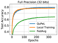
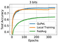
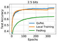
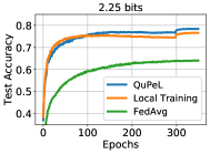
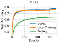
Figure 1: Average test accuracy across clients compared for each scheme for different precision of learned quantization. For QuPeL and Local Training, results are reported for quantized models (except the first plot). For FedAvg we always use full precision global model.

Results. We state our results in Table 2, and provide comparison of average test accuracy across clients in Figure 1 for the different schemes. We compare the schemes for four different cases based on allowed precision for the quantized models: (i) Full precision (32 bit), (ii) (3 bits): each client learns a 3 bit quantization, (iii) (2.75 bits): fifteen clients learn a 3 bits other five learn a 2 bits quantization (iv) (2.5 bits): ten clients learn a 2 bits and the other ten learn 3 bits quantization, (v) (2.25 bits): five clients learn a 3 bits and the rest fifteen learn a 2 bits quantization, (vi) (2 bits): each client learns a 2 bit quantization. In cases (ii)-(vi) for local training, we provide accuracies for quantized models learned using our centralized training scheme (Algorithm 1) without collaboration for a fair comparison. For full precision (32 bit) training, ‘QuPeL’ (see Footnote 6) has 1.5% more accuracy than local training on account of collaboration between clients, while having 15% more accuracy than FedAvg on account of learning personalized models for heterogeneous clients. For learning quantized models (in 3 bits, 2.75 bits, 2.5 bits, 2.25 bits 2 bits cases), our proposed algorithm QuPeL outperforms local training around $1.5-2\%$ on account of collaboration between clients.

Discussion. The above comparison results give insight into two salient features of our training algorithm QuPeL:

Model compression: When learning personalized models, comparison of QuPeL for full precision (32bits) and quantized training shows that using a quantized model for inference does not significantly affect performance. This means that QuPeL can provide personalized, compressed models for deployment which effectively match full precision models in test performance.

Collaboration: Comparison of QuPeL with local training (where clients do not collaborate) shows that collaboration between participating clients (as in QuPeL) can increase the test performance of the learned models. Thus, QuPeL allows clients to leverage information from each other in cases when local data is not sufficient, which can improve the test performance of the learned personalized models.

	Test Accuracy
Collaboration with 2 Bit clients	$78.17\pm 0.11$
Collaboration with 3 Bit clients	$78.79\pm 0.12$

Table 3: Average Test accuracy (in %) of Control Clients.

Collaboration with resource rich clients. We demonstrate that for clients with scarce resources, it is advantageous to collaborate with the clients with more resources in terms of having finer quantized models. To investigate this we choose a subset of 10 out of 20 clients and constraint them to have 2 bits; we call these 10 clients ‘Control Clients’. Then we examine their average test accuracy in two cases, depending on whether the other 10 clients are restricted to have 2-bit or 3-bit quantizers. In Table 3 we observe an increase of $0.62\%$ in test accuracy for the Control Clients. In case of collaboration with full precision clients there are further small gains. This implies, clients with scarce resources can take advantage of clients with rich resources.

8 Conclusion

In this paper, we propose a new problem formulation to enable personalized model compression in a federated setting, where clients also learn different personalized models. For this, we propose and analyze QuPeL, a relaxed optimization framework to learn personalized quantization levels as well as the model parameters. We give first convergence analysis on the QuPeL through this relaxed optimization problem. We observe that QuPeL recovers the convergence rates in the related works on personalized learning, which utilize full precision personalized models. Numerically, we show that model compression does not significantly degrade the performance and collaboration increases the test performance compared to local training. An intriguing preliminary experimental observation is that resource-starved clients can benefit from collaborating with resource rich clients, perhaps promoting "equity". To conclude, our method demonstrates a good numerical performance together with convergence guarantees while accounting for data and resource heterogeneity among clients.

Appendix A Preliminaries

A.1 Notation

• Given a composite function $g({\bf x},{\bf y})$ we will denote $\nabla g({\bf x},{\bf y})$ or $\nabla_{({\bf x},{\bf y})}g({\bf x},{\bf y})$ as the gradient; $\nabla_{\bf x}g({\bf x},{\bf y})$ and $\nabla_{\bf y}g({\bf x},{\bf y})$ as the partial gradients with respect to ${\bf x}$ and ${\bf y}$.

• For a vector ${\bf u}$, $\|{\bf u}\|$ denotes the $\ell_{2}$-norm $\|{\bf u}\|_{2}$. For a matrix ${\bf A}$, $\|{\bf A}\|_{F}$ denotes the Frobenius norm.

• Unless otherwise stated, for a given vector ${\bf x}$, $x_{i}$ denotes the $i^{\prime}th$ element in vector ${\bf x}$; and ${\bf x}_{i}$ denotes that the vector belongs to client $i$. Furthermore, ${\bf x}^{t}_{i}$ denotes a vector that belongs to client $i$ at time $t$.

A.2 Alternating Proximal Steps

We define the following functions: $f:\mathbb{R}^{d}\rightarrow\mathbb{R},\widetilde{Q}:\mathbb{R}^{d+m}\rightarrow\mathbb{R}^{d}$, and we also define $h({\bf x},{\bf c})=f(\widetilde{Q}_{\bf c}({\bf x})),h:\mathbb{R}^{d+m}\rightarrow\mathbb{R}$ where ${\bf x}\in\mathbb{R}^{d}\text{ and }{\bf c}\in\mathbb{R}^{m}$. Note that here $\widetilde{Q}_{\bf c}({\bf x})$ denotes $\widetilde{Q}({\bf x},{\bf c})$. Throughout our paper we will use $\widetilde{Q}_{\bf c}({\bf x})$ to denote $\widetilde{Q}({\bf x},{\bf c})$, in other words both ${\bf c}$ and ${\bf x}$ are inputs to the function $\widetilde{Q}_{\bf c}({\bf x})$. We propose an alternating proximal gradient algorithm. Our updates are as follows:

$${\bf x}^{t+1}=\text{prox}_{\eta_{1}\lambda R(\cdot,{\bf c}^{t})}({\bf x}^{t}-\eta_{1}\nabla f({\bf x}^{t})-\eta_{1}\nabla_{{\bf x}^{t}}f(\widetilde{Q}_{{\bf c}^{t}}({\bf x}^{t})))$$ (42)

$${\bf c}^{t+1}=\text{prox}_{\eta_{2}\lambda R({\bf x}^{t+1},\cdot)}({\bf c}^{t}-\eta_{2}\nabla_{{\bf c}^{t}}f(\widetilde{Q}_{{\bf c}^{t}}({\bf x}^{t+1})))$$

For simplicity we assume the functions in the objective function are differentiable, however, our analysis could also be done using subdifferentials.

Our method is inspired by (Bolte et al., 2014) where the authors introduce an alternating proximal minimization algorithm to solve a broad class of non-convex problems as an alternative to coordinate descent methods. In this work we construct another optimization problem that can be used as a surrogate in learning quantized networks where both model parameters and quantization levels are subject to optimization. In particular, Bolte et al. (2014) considers a general objective function of the form $F({\bf x},{\bf y})=f({\bf x})+g({\bf y})+\lambda H({\bf x},{\bf y})$, whereas, our objective function is tailored for learning quantized networks: $F_{\lambda}({\bf x},{\bf c})=f({\bf x})+f(\widetilde{Q}_{{\bf c}}({\bf x}))+\lambda R({\bf x},{\bf c})$. Furthermore, they consider updates where the proximal mappings are with respect to functions $f,g$, whereas in our case the proximal mappings are with respect to the distance function $R({\bf x},{\bf c})$ to capture the soft projection.

A.3 Lipschitz Relations

In this section we will use the assumptions A.1-5 and show useful relations for partial gradients derived from the assumptions. We have the following gradient for the composite function:

$$\nabla_{({\bf x},{\bf c})}h({\bf x},{\bf c})=\nabla_{({\bf x},{\bf c})}f(\widetilde{Q}_{\bf c}({\bf x}))=\nabla_{({\bf x},{\bf c})}\widetilde{Q}_{\bf c}({\bf x})\nabla_{\widetilde{Q}_{\bf c}({\bf x})}f(\widetilde{Q}_{\bf c}({\bf x}))$$ (43)

where $dim(\nabla h({\bf x},{\bf c}))=(d+m)\times 1,\ dim(\nabla_{\widetilde{Q}_{\bf c}({\bf x})}f(\widetilde{Q}_{\bf c}({\bf x})))=d\times 1,\ dim(\nabla\widetilde{Q}_{\bf c}({\bf x}))=(d+m)\times d$. Note that the soft quantization functions of our interest are elementwise which implies $\frac{\partial\widetilde{Q}_{\bf c}({\bf x})_{i}}{\partial x_{j}}=0$ if $i\neq j$. In particular, for the gradient of the quantization function we have,

$$\nabla_{({\bf x},{\bf c})}\widetilde{Q}_{\bf c}({\bf x})=\begin{bmatrix}\frac{\partial\widetilde{Q}_{\bf c}({\bf x})_{1}}{\partial x_{1}}&0&\ldots\\ 0&\frac{\partial\widetilde{Q}_{\bf c}({\bf x})_{2}}{\partial x_{2}}&0\ldots\\ \vdots&\vdots&\vdots\\ \frac{\partial\widetilde{Q}_{\bf c}({\bf x})_{1}}{\partial c_{1}}&\frac{\partial\widetilde{Q}_{\bf c}({\bf x})_{2}}{\partial c_{1}}&\ldots\\ \vdots&\vdots&\vdots\\ \frac{\partial\widetilde{Q}_{\bf c}({\bf x})_{1}}{\partial c_{m}}&\frac{\partial\widetilde{Q}_{\bf c}({\bf x})_{2}}{\partial c_{m}}&\ldots\end{bmatrix}$$ (44)

Moreover for the composite function we have,

$$\nabla h({\bf x},{\bf c})=\begin{bmatrix}&\frac{\partial f}{\partial\widetilde{Q}_{\bf c}({\bf x})_{1}}\frac{\partial\widetilde{Q}_{\bf c}({\bf x})_{1}}{\partial x_{1}}&+0&+\ldots\\ &0&+\frac{\partial f}{\partial\widetilde{Q}_{\bf c}({\bf x})_{2}}\frac{\partial\widetilde{Q}_{\bf c}({\bf x})_{2}}{\partial x_{2}}&+\ldots\\ &\vdots\\ &\frac{\partial f}{\partial\widetilde{Q}_{\bf c}({\bf x})_{1}}\frac{\partial\widetilde{Q}_{\bf c}({\bf x})_{1}}{\partial c_{1}}&+\frac{\partial f}{\partial\widetilde{Q}_{\bf c}({\bf x})_{2}}\frac{\partial\widetilde{Q}_{\bf c}({\bf x})_{2}}{\partial c_{1}}&+\ldots\\ &\vdots\\ &\frac{\partial f}{\partial\widetilde{Q}_{\bf c}({\bf x})_{1}}\frac{\partial\widetilde{Q}_{\bf c}({\bf x})_{1}}{\partial c_{m}}&+\frac{\partial f}{\partial\widetilde{Q}_{\bf c}({\bf x})_{2}}\frac{\partial\widetilde{Q}_{\bf c}({\bf x})_{2}}{\partial c_{m}}&+\ldots\end{bmatrix}$$ (45)

In (45) and (44) we use $x_{i}$, $c_{j}$ to denote $({\bf x})_{i}$ and $({\bf c})_{j}$ (i’th, j’th element respectively) for notational simplicity. Now, we prove two claims that will be useful in the main analysis.

Claim 10.

$$\|\nabla_{\bf x}f(\widetilde{Q}_{\bf c}({\bf x}))-\nabla_{\bf y}f(\widetilde{Q}_{\bf c}({\bf y}))\|=\|\nabla h({\bf x},{\bf c})_{1:d}-\nabla h({\bf y},{\bf c})_{1:d}\|\leq(GL_{Q_{1}}+G_{Q_{1}}Ll_{Q_{1}})\|{\bf x}-{\bf y}\|$$

Proof.

$$\|\nabla h({\bf x},{\bf c})_{1:d}-\nabla h({\bf y},{\bf c})_{1:d}\| =\|\nabla_{\bf x}f(\widetilde{Q}_{{\bf c}}({\bf x}))-\nabla_{\bf y}f(\widetilde{Q}_{{\bf c}}({\bf y}))\|$$

$$=\|\nabla_{\widetilde{Q}_{\bf c}({\bf x})}f(\widetilde{Q}_{\bf c}({\bf x}))\nabla_{\bf x}\widetilde{Q}_{\bf c}({\bf x})-\nabla_{\widetilde{Q}_{\bf c}({\bf y})}f(\widetilde{Q}_{\bf c}({\bf y}))\nabla_{\bf y}\widetilde{Q}_{\bf c}({\bf y})\|$$

$$=\|\nabla_{\widetilde{Q}_{\bf c}({\bf x})}f(\widetilde{Q}_{\bf c}({\bf x}))\nabla_{\bf x}\widetilde{Q}_{\bf c}({\bf x})-\nabla_{\widetilde{Q}_{\bf c}({\bf x})}f(\widetilde{Q}_{\bf c}({\bf x}))\nabla_{\bf y}\widetilde{Q}_{\bf c}({\bf y})$$

$$\quad+\nabla_{\widetilde{Q}_{\bf c}({\bf x})}f(\widetilde{Q}_{\bf c}({\bf x}))\nabla_{\bf y}\widetilde{Q}_{\bf c}({\bf y})-\nabla_{\widetilde{Q}_{\bf c}({\bf y})}f(\widetilde{Q}_{\bf c}({\bf y}))\nabla_{\bf y}\widetilde{Q}_{\bf c}({\bf y})\|$$

$$\stackrel{{\scriptstyle\text{(a)}}}{{\leq}}\|\nabla_{\widetilde{Q}_{\bf c}({\bf x})}f(\widetilde{Q}_{\bf c}({\bf x}))\|\|\nabla_{\bf x}\widetilde{Q}_{\bf c}({\bf x})-\nabla_{\bf y}\widetilde{Q}_{\bf c}({\bf y})\|_{F}$$

$$\quad+\|\nabla_{\bf y}\widetilde{Q}_{\bf c}({\bf y})\|_{F}\|\nabla_{\widetilde{Q}_{\bf c}({\bf x})}f(\widetilde{Q}_{\bf c}({\bf x}))-\nabla_{\widetilde{Q}_{\bf c}({\bf y})}f(\widetilde{Q}_{\bf c}({\bf y}))\|$$

$$\leq GL_{Q_{1}}\|{\bf x}-{\bf y}\|+G_{Q_{1}}L\|\widetilde{Q}_{\bf c}({\bf x})-\widetilde{Q}_{\bf c}({\bf y})\|$$

$$\leq GL_{Q_{1}}\|{\bf x}-{\bf y}\|+G_{Q_{1}}Ll_{Q_{1}}\|{\bf x}-{\bf y}\|=(GL_{Q_{1}}+G_{Q_{1}}Ll_{Q_{1}})\|{\bf x}-{\bf y}\|$$

To obtain (a) we have used the fact $\|{\bf A}{\bf x}\|_{2}\leq\|{\bf A}\|_{F}\|{\bf x}\|_{2}$. ∎

Claim 11.

$$\|\nabla_{\bf c}f(\widetilde{Q}_{\bf c}({\bf x}))-\nabla_{\bf d}f(\widetilde{Q}_{\bf d}({\bf x}))\|=\|\nabla h({\bf x},{\bf c})_{d+1:m}-\nabla h({\bf x},{\bf d})_{d+1:m}\|\leq(GL_{Q_{2}}+G_{Q_{2}}Ll_{Q_{2}})\|{\bf c}-{\bf d}\|$$

Proof.

We can follow similar steps,

$$\|\nabla h({\bf x},{\bf c})_{d+1:m}-\nabla h({\bf x},{\bf d})_{d+1:m}\| =\|\nabla_{\bf c}f(\widetilde{Q}_{{\bf c}}({\bf x}))-\nabla_{\bf d}f(\widetilde{Q}_{{\bf d}}({\bf x}))\|$$

$$=\|\nabla_{\widetilde{Q}_{\bf c}({\bf x})}f(\widetilde{Q}_{\bf c}({\bf x}))\nabla_{\bf c}\widetilde{Q}_{\bf c}({\bf x})-\nabla_{\widetilde{Q}_{\bf d}({\bf y})}f(\widetilde{Q}_{\bf d}({\bf y}))\nabla_{\bf d}\widetilde{Q}_{\bf d}({\bf y})\|$$

$$=\|\nabla_{\widetilde{Q}_{\bf c}({\bf x})}f(\widetilde{Q}_{\bf c}({\bf x}))\nabla_{\bf c}\widetilde{Q}_{\bf c}({\bf x})-\nabla_{\widetilde{Q}_{\bf c}({\bf x})}f(\widetilde{Q}_{\bf c}({\bf x}))\nabla_{\bf d}\widetilde{Q}_{\bf d}({\bf x})$$

$$\quad+\nabla_{\widetilde{Q}_{\bf c}({\bf x})}f(\widetilde{Q}_{\bf c}({\bf x}))\nabla_{\bf d}\widetilde{Q}_{\bf d}({\bf y})-\nabla_{\widetilde{Q}_{\bf d}({\bf x})}f(\widetilde{Q}_{\bf d}({\bf y}))\nabla_{\bf d}\widetilde{Q}_{\bf d}({\bf y})\|$$

$$\leq\|\nabla_{\widetilde{Q}_{\bf c}({\bf x})}f(\widetilde{Q}_{\bf c}({\bf x}))\|\|\nabla_{\bf c}\widetilde{Q}_{\bf c}({\bf x})-\nabla_{\bf d}\widetilde{Q}_{\bf d}({\bf y})\|_{F}$$

$$\quad+\|\nabla_{\bf d}\widetilde{Q}_{\bf d}({\bf y})\|_{F}\|\nabla_{\widetilde{Q}_{\bf c}({\bf x})}f(\widetilde{Q}_{\bf c}({\bf x}))-\nabla_{\widetilde{Q}_{\bf d}({\bf y})}f(\widetilde{Q}_{\bf d}({\bf y}))\|$$

$$\leq GL_{Q_{2}}\|{\bf c}-{\bf d}\|+G_{Q_{2}}L\|\widetilde{Q}_{\bf c}({\bf x})-\widetilde{Q}_{\bf d}({\bf x})\|$$

$$\leq GL_{Q_{2}}\|{\bf c}-{\bf d}\|+G_{Q_{2}}Ll_{Q_{2}}\|{\bf c}-{\bf d}\|=(GL_{Q_{2}}+G_{Q_{2}}Ll_{Q_{2}})\|{\bf c}-{\bf d}\|$$

where $\nabla_{\bf c}\widetilde{Q}_{\bf c}({\bf x})=\nabla\widetilde{Q}_{\bf c}({\bf x})_{(d+1:d+m,:)}$. ∎

A.4 Proof of the Claims Regarding Soft Quantization Function

Claim (Restating Claim 1).

$\widetilde{Q}_{\bf c}({\bf x})$ is $l_{Q_{1}}$-Lipschitz continuous and $L_{Q_{1}}$-smooth with respect to ${\bf x}$.

Proof.

First we prove Lipschitz continuity. Note,

$$\frac{\partial\widetilde{Q}_{\bf c}({\bf x})_{i}}{\partial x_{j}}=\begin{cases}0,\text{ if }i\neq j\\ P\sum_{j=2}^{m}(c_{j}-c_{j-1})\sigma(P(x_{i}-\frac{c_{j}+c_{j-1}}{2}))(1-\sigma(P(x_{i}-\frac{c_{j}+c_{j-1}}{2}))),\text{ if }i=j\\ \end{cases}$$ (46)

As a result, $\|\frac{\partial\widetilde{Q}_{\bf c}({\bf x})_{i}}{\partial x_{j}}\|\leq\frac{P}{4}(c_{m}-c_{1})\leq\frac{P}{2}c_{max}$. The norm of the gradient of $\widetilde{Q}_{\bf c}({\bf x})_{i}$ with respect to $x$ is bounded which implies there exists $l^{(i)}_{Q_{1}}$ such that $\|\widetilde{Q}_{\bf c}({\bf x})_{i}-\widetilde{Q}_{\bf c}({\bf x}^{\prime})_{i}\|\leq l^{(i)}_{Q_{1}}\|{\bf x}-{\bf x}^{\prime}\|$; using Fact 5 and the fact that $i$ was arbitrary, there exists $l_{Q_{1}}$ such that $\|\widetilde{Q}_{\bf c}({\bf x})-\widetilde{Q}_{\bf c}({\bf x}^{\prime})\|\leq l_{Q_{1}}\|{\bf x}-{\bf x}^{\prime}\|$. In other words, $\widetilde{Q}_{\bf c}({\bf x})$ is Lipschitz continuous.

For smoothness note that, $\nabla_{\bf x}\widetilde{Q}_{\bf c}({\bf x})=\nabla\widetilde{Q}_{\bf c}({\bf x})_{1:d,:}$. Now we focus on an arbitrary term of $\nabla_{\bf x}\widetilde{Q}_{\bf c}({\bf x})_{j,i}$. From (46) we know that this term is 0 if $i\neq j$, and a weighted sum of product of sigmoid functions if $i=j$. Then, using the Facts 1-4 the function $\nabla_{\bf x}\widetilde{Q}_{\bf c}({\bf x})_{j,i}$ is Lipschitz continuous. Since $i,j$ were arbitrarily chosen, $\nabla_{\bf x}\widetilde{Q}_{\bf c}({\bf x})_{j,i}$ is Lipschitz continuous for all $i,j$. Then, by Fact 5, $\nabla_{\bf x}\widetilde{Q}_{\bf c}({\bf x})$ is Lipschitz continuous, which implies that $\widetilde{Q}_{\bf c}({\bf x})$ is $L_{Q_{1}}$-smooth for some coefficient $L_{Q_{1}}<\infty$. ∎

Claim (Restating Claim 2).

$\widetilde{Q}_{\bf c}({\bf x})$ is $l_{Q_{2}}$-Lipschitz continuous and $L_{Q_{2}}$-smooth with respect to ${\bf c}$.

Proof.

For Lipschitz continuity we have,

$$\frac{\partial\widetilde{Q}_{\bf c}({\bf x})_{i}}{\partial c_{j}} =\sigma(P(x_{i}-\frac{c_{j}+c_{j-1}}{2}))-\sigma(P(x_{i}-\frac{c_{j}+c_{j+1}}{2}))$$

$$\quad+(c_{j}-c_{j+1})\frac{P}{2}\sigma(P(x_{i}-\frac{c_{j}+c_{j+1}}{2}))(1-\sigma(P(x_{i}-\frac{c_{j}+c_{j+1}}{2})))$$

$$\quad-(c_{j}-c_{j-1})\frac{P}{2}\sigma(P(x_{i}-\frac{c_{j}+c_{j-1}}{2}))(1-\sigma(P(x_{i}-\frac{c_{j}+c_{j-1}}{2})))$$

As a result, $\|\frac{\partial\widetilde{Q}_{\bf c}({\bf x})_{i}}{\partial c_{j}}\|\leq 2+c_{max}\frac{P}{2}$. Similar to Claim 1 using the facts that $i$ is arbitrary and the Fact 5, we find there exists $l_{Q_{2}}$ such that $\|\widetilde{Q}_{\bf c}({\bf x})-\widetilde{Q}_{\bf d}({\bf x})\|\leq l_{Q_{1}}\|{\bf c}-{\bf d}\|$. In other words, $\widetilde{Q}_{\bf c}({\bf x})$ is Lipschitz continuous. And for the smoothness, following the same idea from the proof of Claim 2 we find $\widetilde{Q}_{\bf c}({\bf x})$ is $L_{Q_{2}}$-smooth with respect to ${\bf c}$. ∎

Appendix B Omitted Details from Section 5 – Proof of Theorem 1

First we derive the optimization problems that the alternating updates correspond to. Remember we had the following alternating updates:

$${\bf x}^{t+1}=\text{prox}_{\eta_{1}\lambda R_{{\bf c}^{t}}}({\bf x}^{t}-\eta_{1}\nabla f({\bf x}^{t})-\eta_{1}\nabla_{{\bf x}^{t}}f(\widetilde{Q}_{{\bf c}^{t}}({\bf x}^{t})))$$

$${\bf c}^{t+1}=\text{prox}_{\eta_{2}\lambda R_{{\bf x}^{t+1}}}({\bf c}^{t}-\eta_{2}\nabla_{{\bf c}^{t}}f(\widetilde{Q}_{{\bf c}^{t}}({\bf x}^{t+1})))$$

For ${\bf x}^{t+1}$, from the definition of proximal mapping we have:

$${\bf x}^{t+1} =\underset{{\bf x}\in\mathbb{R}^{d}}{\arg\min}\left\{\frac{1}{2\eta_{1}}\left\|{\bf x}-{\bf x}^{t}+\eta_{1}\nabla_{{\bf x}^{t}}f\left({\bf x}^{t}\right)+\eta_{1}\nabla_{{\bf x}^{t}}f(\widetilde{Q}_{{\bf c}^{t}}({\bf x}^{t}))\right\|_{2}^{2}+\lambda R({\bf x},{\bf c}^{t})\right\}$$

$$=\underset{{\bf x}\in\mathbb{R}^{d}}{\arg\min}\Big{\{}\left\langle{\bf x}-{\bf x}^{t},\nabla_{{\bf x}^{t}}f\left({\bf x}^{t}\right)\right\rangle+\left\langle{\bf x}-{\bf x}^{t},\nabla_{{\bf x}^{t}}f(\widetilde{Q}_{{\bf c}^{t}}({\bf x}^{t}))\right\rangle+\frac{1}{2\eta_{1}}\left\|{\bf x}-{\bf x}^{t}\right\|_{2}^{2}+\frac{\eta_{1}}{2}\|\nabla_{{\bf x}^{t}}f({\bf x}^{t})+\nabla_{{\bf x}^{t}}f(\widetilde{Q}_{{\bf c}^{t}}({\bf x}^{t}))\|^{2}$$

$$+\lambda R({\bf x},{\bf c}^{t})\Big{\}}$$

$$=\underset{{\bf x}\in\mathbb{R}^{d}}{\arg\min}\left\{\left\langle{\bf x}-{\bf x}^{t},\nabla_{{\bf x}^{t}}f\left({\bf x}^{t}\right)\right\rangle+\left\langle{\bf x}-{\bf x}^{t},\nabla_{{\bf x}^{t}}f(\widetilde{Q}_{{\bf c}^{t}}({\bf x}^{t}))\right\rangle+\frac{1}{2\eta_{1}}\left\|{\bf x}-{\bf x}^{t}\right\|_{2}^{2}+\lambda R({\bf x},{\bf c}^{t})\right\}$$ (47)

Note, in the third equality we remove the terms that do not depend on ${\bf x}$. Similarly, for ${\bf c}^{t+1}$ we have:

$${\bf c}^{t+1} =\underset{{\bf c}\in\mathbb{R}^{m}}{\arg\min}\left\{\frac{1}{2\eta_{2}}\left\|{\bf c}-{\bf c}^{t}+\eta_{2}\nabla_{{\bf c}^{t}}f(\widetilde{Q}_{{\bf c}^{t}}({\bf x}^{t+1}))\right\|_{2}^{2}+\lambda R({\bf x}^{t+1},{\bf c})\right\}$$

$$=\underset{{\bf c}\in\mathbb{R}^{m}}{\arg\min}\left\{\left\langle{\bf c}-{\bf c}^{t},\nabla_{{\bf c}^{t}}f(\widetilde{Q}_{{\bf c}^{t}}({\bf x}^{t+1}))\right\rangle+\frac{1}{2\eta_{2}}\left\|{\bf c}-{\bf c}^{t}\right\|_{2}^{2}+\frac{\eta_{2}}{2}\|\nabla_{{\bf c}^{t}}f(\widetilde{Q}_{{\bf c}^{t}}({\bf x}^{t+1}))\|^{2}+\lambda R({\bf x}^{t+1},{\bf c})\right\}$$

$$=\underset{{\bf c}\in\mathbb{R}^{m}}{\arg\min}\left\{\left\langle{\bf c}-{\bf c}^{t},\nabla_{{\bf c}^{t}}f(\widetilde{Q}_{{\bf c}^{t}}({\bf x}^{t+1}))\right\rangle+\frac{1}{2\eta_{2}}\left\|{\bf c}-{\bf c}^{t}\right\|_{2}^{2}+\lambda R({\bf x}^{t+1},{\bf c})\right\}$$ (48)

Minimization problems in (B) and (B) are the main problems to characterize the update rules and we use them in multiple places throughout the section.

B.1 Proof of the Claims

Claim (Restating Claim 3).

$f({\bf x})+f(\widetilde{Q}_{\bf c}({\bf x}))$ is $(L+GL_{Q_{1}}+G_{Q_{1}}LL_{Q_{1}})$-smooth with respect to ${\bf x}$.

Proof.

From our assumptions, we have $f$ is $L$-smooth. And from Claim 10 we have $f(\widetilde{Q}_{\bf c}({\bf x}))$ is $(GL_{Q_{1}}+G_{Q_{1}}LL_{Q_{1}})$-smooth. Using the fact that if two functions $g_{1}$ and $g_{2}$ are $L_{1}$ and $L_{2}$ smooth respectively, then $g_{1}+g_{2}$ is $(L_{1}+L_{2})$-smooth concludes the proof. ∎

Claim (Restating Claim 4).

Let

$$A({\bf x}^{t+1}) :=\lambda R({\bf x}^{t+1},{\bf c}^{t})+\left\langle\nabla f({\bf x}^{t}),{\bf x}^{t+1}-{\bf x}^{t}\right\rangle+\left\langle\nabla_{{\bf x}^{t}}f(\widetilde{Q}_{{\bf c}^{t}}({\bf x}^{t})),{\bf x}^{t+1}-{\bf x}^{t}\right\rangle+\frac{1}{2\eta_{1}}\|{\bf x}^{t+1}-{\bf x}^{t}\|^{2}$$

$$A({\bf x}^{t}) :=\lambda R({\bf x}^{t},{\bf c}^{t}).$$

Then $A({\bf x}^{t+1})\leq A({\bf x}^{t})$.

Proof.

Let $A({\bf x})$ denote the expression inside the $\arg\min$ in (B) and we know that (B) is minimized when ${\bf x}={\bf x}^{t+1}$. So we have $A({\bf x}^{t+1})\leq A({\bf x}^{t})$. This proves the claim. ∎

Claim (Restating Claim 5).

Let

$$B({\bf c}^{t+1}) :=\lambda R({\bf x}^{t+1},{\bf c}^{t+1})+\left\langle\nabla_{{\bf c}^{t}}f(\widetilde{Q}_{{\bf c}^{t}}({\bf x}^{t+1})),{\bf c}^{t+1}-{\bf c}^{t}\right\rangle+\frac{1}{2\eta_{1}}\|{\bf c}^{t+1}-{\bf c}^{t}\|^{2}$$

$$B({\bf c}^{t}) :=\lambda R({\bf x}^{t+1},{\bf c}^{t}).$$

Then $B({\bf c}^{t+1})\leq B({\bf c}^{t})$.

Proof.

Let $B({\bf c})$ denote the expression inside the $\arg\min$ in (B) and we know that (B) is minimized when ${\bf c}={\bf c}^{t+1}$. So we have $B({\bf c}^{t+1})\leq B({\bf c}^{t})$. This proves the claim. ∎

Appendix C Omitted Details from Section 6 – Proof of Theorem 2

Again we begin with deriving the optimization problems that alternating proximal updates correspond to. The update rule for ${\bf x}^{t}_{i}$ is

$${\bf x}^{t+1}_{i} =\text{prox}_{\eta_{1}\lambda R_{{\bf c}^{t}_{i}}}({\bf x}^{t}_{i}-\eta_{1}\nabla f_{i}({\bf x}^{t}_{i})-\eta_{1}\nabla_{{\bf x}^{t}_{i}}f_{i}(\widetilde{Q}_{{\bf c}^{t}_{i}}({\bf x}^{t}_{i}))-\eta_{1}\lambda_{p}({\bf x}^{t}_{i}-{\bf w}^{t}_{i}))$$

$$=\underset{{\bf x}\in\mathbb{R}^{d}}{\arg\min}\left\{\frac{1}{2\eta_{1}}\left\|{\bf x}-{\bf x}^{t}_{i}+\eta_{1}\nabla f_{i}({\bf x}^{t}_{i})+\eta_{1}\nabla_{{\bf x}^{t}_{i}}f_{i}(\widetilde{Q}_{{\bf c}^{t}_{i}}({\bf x}^{t}_{i}))+\eta_{1}\lambda_{p}({\bf x}^{t}_{i}-{\bf w}^{t}_{i})\right\|^{2}+\lambda R({\bf x},{\bf c}^{t}_{i})\right\}$$

$$=\underset{{\bf x}\in\mathbb{R}^{d}}{\arg\min}\left\{\left\langle{\bf x}-{\bf x}^{t}_{i},\nabla f_{i}\left({\bf x}^{t}_{i}\right)\right\rangle+\left\langle{\bf x}-{\bf x}^{t}_{i},\nabla_{{\bf x}^{t}_{i}}f_{i}(\widetilde{Q}_{{\bf c}^{t}_{i}}({\bf x}^{t}_{i}))\right\rangle+\left\langle{\bf x}-{\bf x}^{t}_{i},\lambda_{p}({\bf x}^{t}_{i}-{\bf w}^{t}_{i})\right\rangle\right.$$

$$\hskip 256.0748pt\left.+\frac{1}{2\eta_{1}}\left\|{\bf x}-{\bf x}^{t}_{i}\right\|_{2}^{2}+\lambda R({\bf x},{\bf c}^{t}_{i})\right\}$$ (49)

and the update rule for ${\bf c}^{t}_{i}$ is

$${\bf c}^{t+1}_{i} =\text{prox}_{\eta_{2}\lambda R_{{\bf x}^{t+1}_{i}}}({\bf c}^{t}_{i}-\eta_{2}\nabla_{{\bf c}^{t}_{i}}f_{i}(\widetilde{Q}_{{\bf c}^{t}_{i}}({\bf x}^{t}_{i})))$$

$$=\underset{{\bf c}\in\mathbb{R}^{m}}{\arg\min}\left\{\frac{1}{2\eta_{2}}\left\|{\bf c}-{\bf c}^{t}_{i}+\eta_{2}\nabla_{{\bf c}^{t}_{i}}f_{i}(\widetilde{Q}_{{\bf c}^{t}_{i}}({\bf x}^{t+1}_{i}))\right\|^{2}+\lambda R({\bf x}^{t+1}_{i},{\bf c})\right\}$$

$$=\underset{{\bf c}\in\mathbb{R}^{m}}{\arg\min}\left\{\left\langle{\bf c}-{\bf c}^{t}_{i},\nabla_{{\bf c}^{t}_{i}}f_{i}(\widetilde{Q}_{{\bf c}^{t}_{i}}({\bf x}^{t+1}_{i}))\right\rangle\right.\left.+\frac{1}{2\eta_{2}}\left\|{\bf c}-{\bf c}^{t}_{i}\right\|_{2}^{2}+\lambda R({\bf x}^{t+1}_{i},{\bf c})\right\}$$ (50)

C.1 Proof of the Claims

Claim (Restating Claim 6).

$f_{i}({\bf x})+f_{i}(\widetilde{Q}_{\bf c}({\bf x}))+\frac{\lambda_{p}}{2}\|{\bf x}-{\bf w}\|^{2}$ is $(\lambda_{p}+L+GL_{Q_{1}}+G_{Q_{1}}LL_{Q_{1}})$-smooth with respect to ${\bf x}$.

Proof.

From our assumptions, we have $f_{i}$ is $L$-smooth. We know $\frac{\lambda_{p}}{2}\|{\bf x}-{\bf w}\|^{2}$ is $\lambda_{p}$-smooth with respect to ${\bf x}$. And applying the Claim 10 to each client separately gives that $f_{i}(\widetilde{Q}_{\bf c}({\bf x}))$ is $(GL_{Q_{1}}+G_{Q_{1}}LL_{Q_{1}})$-smooth. Using the fact that if two functions $g_{1}$ and $g_{2}$ are $L_{1}$ and $L_{2}$ smooth respectively, then $g_{1}+g_{2}$ is $(L_{1}+L_{2})$-smooth concludes the proof. ∎

Claim (Restating Claim 7).

Let

$$A({\bf x}^{t+1}_{i}) :=\lambda R({\bf x}^{t+1}_{i},{\bf c}^{t}_{i})+\left\langle\nabla f_{i}({\bf x}^{t}_{i}),{\bf x}^{t+1}_{i}-{\bf x}^{t}_{i}\right\rangle+\left\langle\nabla_{{\bf x}^{t}_{i}}f_{i}(\widetilde{Q}_{{\bf c}^{t}_{i}}({\bf x}^{t}_{i})),{\bf x}^{t+1}_{i}-{\bf x}^{t}_{i}\right\rangle$$

$$\hskip 85.35826pt+\left\langle\lambda_{p}({\bf x}^{t}_{i}-{\bf w}^{t}_{i}),{\bf x}^{t+1}_{i}-{\bf x}^{t}_{i}\right\rangle+\frac{1}{2\eta_{1}}\|{\bf x}^{t+1}_{i}-{\bf x}^{t}_{i}\|^{2}$$

$$A({\bf x}^{t}_{i}) :=\lambda R({\bf x}^{t}_{i},{\bf c}^{t}_{i}).$$

Then $A({\bf x}^{t+1}_{i})\leq A({\bf x}^{t}_{i})$.

Proof.

Let $A({\bf x})$ denote the expression inside the $\arg\min$ in (49) and we know that (49) is minimized when ${\bf x}={\bf x}^{t+1}_{i}$. So we have $A({\bf x}^{t+1}_{i})\leq A({\bf x}^{t}_{i})$. This proves the claim. ∎

Claim (Restating Claim 8).

$(GL_{Q_{2}}+G_{Q_{2}}LL_{Q_{2}})$-smooth with respect to ${\bf c}$.

Proof.

Applying the Claim 11 to each client separately gives that $f_{i}(\widetilde{Q}_{\bf c}({\bf x}))$ is $(GL_{Q_{2}}+G_{Q_{2}}LL_{Q_{2}})$-smooth. ∎

Claim (Restating Claim 9).

Let

$$B({\bf c}^{t+1}_{i}) :=\lambda R({\bf x}^{t+1}_{i},{\bf c}^{t+1}_{i})+\left\langle\nabla_{{\bf c}^{t}_{i}}f_{i}(\widetilde{Q}_{{\bf c}^{t}_{i}}({\bf x}^{t+1}_{i})),{\bf c}^{t+1}_{i}-{\bf c}^{t}_{i}\right\rangle+\frac{1}{2\eta_{2}}\|{\bf c}^{t+1}_{i}-{\bf c}^{t}_{i}\|^{2}$$

$$B({\bf c}^{t}_{i}) :=\lambda R({\bf x}^{t+1}_{i},{\bf c}^{t}_{i}).$$

Then $B({\bf c}^{t+1}_{i})\leq B({\bf c}^{t}_{i})$.

Proof.

Note that the update rule for ${\bf c}$ is: Let $B({\bf c})$ denote the expression inside the $\arg\min$ in (50) and we know that (50) is minimized when ${\bf c}={\bf c}^{t+1}_{i}$. So we have $B({\bf c}^{t+1}_{i})\leq B({\bf c}^{t}_{i})$. This proves the claim. ∎

Obtaining (6.1.3). Note, we have $F_{i}({\bf x}.{\bf c},{\bf w})$ is $\lambda_{p}$-smooth w.r.t ${\bf w}$. Then,

$$F_{i}({\bf x}^{t+1}_{i},{\bf c}^{t+1}_{i},{\bf w}^{t+1}) \leq F_{i}({\bf x}^{t+1}_{i},{\bf c}^{t+1}_{i},{\bf w}^{t})+\left\langle\nabla_{{\bf w}^{t}}F_{i}({\bf x}^{t+1}_{i},{\bf c}^{t+1}_{i},{\bf w}^{t}),{\bf w}^{t+1}-{\bf w}^{t}\right\rangle+\frac{\lambda_{p}}{2}\|{\bf w}^{t+1}-{\bf w}^{t}\|^{2}$$

$$=F_{i}({\bf x}^{t+1}_{i},{\bf c}^{t+1}_{i},{\bf w}^{t})+\left\langle\nabla_{{\bf w}^{t}}F_{i}({\bf x}^{t+1}_{i},{\bf c}^{t+1}_{i},{\bf w}^{t}),\eta_{3}{\bf g}^{t}\right\rangle+\frac{\lambda_{p}}{2}\|\eta_{3}{\bf g}^{t}\|^{2}$$

$$=F_{i}({\bf x}^{t+1}_{i},{\bf c}^{t+1}_{i},{\bf w}^{t})$$

$$\quad-\eta_{3}\left\langle\nabla_{{\bf w}^{t}}F_{i}({\bf x}^{t+1}_{i},{\bf c}^{t+1}_{i},{\bf w}^{t}),{\bf g}^{t}-\nabla_{{\bf w}^{t}}F_{i}({\bf x}^{t+1}_{i},{\bf c}^{t+1}_{i},{\bf w}^{t})+\nabla_{{\bf w}^{t}}F_{i}({\bf x}^{t+1}_{i},{\bf c}^{t+1}_{i},{\bf w}^{t})\right\rangle$$

$$\quad+\frac{\lambda_{p}}{2}\eta_{3}^{2}\|{\bf g}^{t}-\nabla_{{\bf w}^{t}}F_{i}({\bf x}^{t+1}_{i},{\bf c}^{t+1}_{i},{\bf w}^{t})+\nabla_{{\bf w}^{t}}F_{i}({\bf x}^{t+1}_{i},{\bf c}^{t+1}_{i},{\bf w}^{t})\|^{2}$$

$$=F_{i}({\bf x}^{t+1}_{i},{\bf c}^{t+1}_{i},{\bf w}^{t})-\eta_{3}\Big{\|}\nabla_{{\bf w}^{t}}F_{i}({\bf x}^{t+1}_{i},{\bf c}^{t+1}_{i},{\bf w}^{t})\Big{\|}^{2}$$

$$\quad-\eta_{3}\left\langle\nabla_{{\bf w}^{t}}F_{i}({\bf x}^{t+1}_{i},{\bf c}^{t+1}_{i},{\bf w}^{t}),{\bf g}^{t}-\nabla_{{\bf w}^{t}}F_{i}({\bf x}^{t+1}_{i},{\bf c}^{t+1}_{i},{\bf w}^{t})\right\rangle$$

$$\quad+\frac{\lambda_{p}}{2}\eta_{3}^{2}\|{\bf g}^{t}-\nabla_{{\bf w}^{t}}F_{i}({\bf x}^{t+1}_{i},{\bf c}^{t+1}_{i},{\bf w}^{t})+\nabla_{{\bf w}^{t}}F_{i}({\bf x}^{t+1}_{i},{\bf c}^{t+1}_{i},{\bf w}^{t})\|^{2}$$

$$\leq F_{i}({\bf x}^{t+1}_{i},{\bf c}^{t+1}_{i},{\bf w}^{t})-\eta_{3}\Big{\|}\nabla_{{\bf w}^{t}}F_{i}({\bf x}^{t+1}_{i},{\bf c}^{t+1}_{i},{\bf w}^{t})\Big{\|}^{2}+\frac{\eta_{3}}{2}\Big{\|}\nabla_{{\bf w}^{t}}F_{i}({\bf x}^{t+1}_{i},{\bf c}^{t+1}_{i},{\bf w}^{t})\Big{\|}^{2}$$

$$\quad+\frac{\eta_{3}}{2}\Big{\|}{\bf g}^{t}-\nabla_{{\bf w}^{t}}F_{i}({\bf x}^{t+1}_{i},{\bf c}^{t+1}_{i},{\bf w}^{t})\Big{\|}^{2}+\lambda_{p}\eta_{3}^{2}\Big{\|}{\bf g}^{t}-\nabla_{{\bf w}^{t}}F_{i}({\bf x}^{t+1}_{i},{\bf c}^{t+1}_{i},{\bf w}^{t})\Big{\|}^{2}$$

$$\quad+\lambda_{p}\eta_{3}^{2}\Big{\|}\nabla_{{\bf w}^{t}}F_{i}({\bf x}^{t+1}_{i},{\bf c}^{t+1}_{i},{\bf w}^{t})\Big{\|}^{2}$$

$$=F_{i}({\bf x}^{t+1}_{i},{\bf c}^{t+1}_{i},{\bf w}^{t})-(\frac{\eta_{3}}{2}-\lambda_{p}\eta_{3}^{2})\Big{\|}\nabla_{{\bf w}^{t}}F_{i}({\bf x}^{t+1}_{i},{\bf c}^{t+1}_{i},{\bf w}^{t})\Big{\|}^{2}$$

$$\quad+(\frac{\eta_{3}}{2}+\lambda_{p}\eta_{3}^{2})\Big{\|}{\bf g}^{t}-\nabla_{{\bf w}^{t}_{i}}F_{i}({\bf x}^{t+1}_{i},{\bf c}^{t+1}_{i},{\bf w}^{t}_{i})+\nabla_{{\bf w}^{t}_{i}}F_{i}({\bf x}^{t+1}_{i},{\bf c}^{t+1}_{i},{\bf w}^{t}_{i})$$

$$\quad-\nabla_{{\bf w}^{t}}F_{i}({\bf x}^{t+1}_{i},{\bf c}^{t+1}_{i},{\bf w}^{t})\Big{\|}^{2}$$

$$\leq F_{i}({\bf x}^{t+1}_{i},{\bf c}^{t+1}_{i},{\bf w}^{t})-(\frac{\eta_{3}}{2}-\lambda_{p}\eta_{3}^{2})\Big{\|}\nabla_{{\bf w}^{t}}F_{i}({\bf x}^{t+1}_{i},{\bf c}^{t+1}_{i},{\bf w}^{t})\Big{\|}^{2}$$

$$\quad+(\eta_{3}+2\lambda_{p}\eta_{3}^{2})\Big{\|}{\bf g}^{t}-\nabla_{{\bf w}^{t}_{i}}F_{i}({\bf x}^{t+1}_{i},{\bf c}^{t+1}_{i},{\bf w}^{t}_{i})\Big{\|}^{2}+(\eta_{3}+2\lambda_{p}\eta_{3}^{2})\Big{\|}\nabla_{{\bf w}^{t}_{i}}F_{i}({\bf x}^{t+1}_{i},{\bf c}^{t+1}_{i},{\bf w}^{t}_{i})$$

$$\quad-\nabla_{{\bf w}^{t}}F_{i}({\bf x}^{t+1}_{i},{\bf c}^{t+1}_{i},{\bf w}^{t})\Big{\|}^{2}$$

$$\leq F_{i}({\bf x}^{t+1}_{i},{\bf c}^{t+1}_{i},{\bf w}^{t})-(\frac{\eta_{3}}{2}-\lambda_{p}\eta_{3}^{2})\Big{\|}\nabla_{{\bf w}^{t}}F_{i}({\bf x}^{t+1}_{i},{\bf c}^{t+1}_{i},{\bf w}^{t})\Big{\|}^{2}$$

$$\quad+(\eta_{3}+2\lambda_{p}\eta_{3}^{2})\Big{\|}{\bf g}^{t}-\nabla_{{\bf w}^{t}_{i}}F_{i}({\bf x}^{t+1}_{i},{\bf c}^{t+1}_{i},{\bf w}^{t}_{i})\Big{\|}^{2}+(\eta_{3}+2\lambda_{p}\eta_{3}^{2})\lambda_{p}^{2}\Big{\|}{\bf w}^{t}_{i}-{\bf w}^{t}\Big{\|}^{2}$$

Hence, we obtain the bound in (6.1.3).

C.2 Proof of Lemma 1 and Corollary 1

Let us restate and prove Lemma 1,

Lemma (Restating Lemma 1).

$$\frac{1}{T}\sum_{t=0}^{T-1}\frac{1}{n}\sum_{i=1}^{n}\|{\bf w}^{t}-{\bf w}^{t}_{i}\|\leq 6\tau^{2}\eta_{3}^{2}\kappa$$ (51)

Proof.

Let $t_{c}$ be the latest synchronization time before t. Define $\gamma_{t}=\frac{1}{n}\sum_{i=1}^{n}\|{\bf w}^{t}-{\bf w}^{t}_{i}\|^{2}$. Then:

$$\gamma_{t} =\frac{1}{n}\sum_{i=1}^{n}\Big{\|}{\bf w}^{tc}-\frac{\eta_{3}}{n}\sum_{j=t_{c}}^{t}\sum_{k=1}^{n}\nabla_{{\bf w}^{j}_{k}}F_{k}({\bf x}^{j+1}_{k},{\bf c}^{j+1}_{k},{\bf w}^{j}_{k}-({\bf w}^{tc}-\eta_{3}\sum_{j=t_{c}}^{t}\nabla_{{\bf w}^{j}_{i}}F_{i}({\bf x}^{j+1}_{i},{\bf c}^{j+1}_{i},{\bf w}^{j}_{i})\Big{\|}^{2}$$

$$\stackrel{{\scriptstyle\text{(a)}}}{{\leq}}\tau\sum_{j=t_{c}}^{t}\frac{\eta_{3}^{2}}{n}\sum_{i=1}^{n}\Big{\|}\frac{1}{n}\sum_{k=1}^{n}\nabla_{{\bf w}^{j}_{k}}F_{k}({\bf x}^{j+1}_{k},{\bf c}^{j+1}_{k},{\bf w}^{j}_{k}-\nabla_{{\bf w}^{j}_{i}}F_{i}({\bf x}^{j+1}_{i},{\bf c}^{j+1}_{i},{\bf w}^{j}_{i}\Big{\|}^{2} \star 1$$ ()

$$=\tau\sum_{j=t_{c}}^{t}\frac{\eta_{3}^{2}}{n}\sum_{i=1}^{n}\Big{[}\Big{\|}\frac{1}{n}\sum_{k=1}^{n}\left(\nabla_{{\bf w}^{j}_{k}}F_{k}({\bf x}^{j+1}_{k},{\bf c}^{j+1}_{k},{\bf w}^{j}_{k})-\nabla_{{\bf w}^{j}}F_{k}({\bf x}^{j+1}_{k},{\bf c}^{j+1}_{k},{\bf w}^{j})+\nabla_{{\bf w}^{j}}F_{k}({\bf x}^{j+1}_{k},{\bf c}^{j+1}_{k},{\bf w}^{j})\right)$$

$$\hskip 56.9055pt-\nabla_{{\bf w}^{j}}F_{i}({\bf x}^{j+1}_{k},{\bf c}^{j+1}_{k},{\bf w}^{j})+\nabla_{{\bf w}^{j}}F_{i}({\bf x}^{j+1}_{k},{\bf c}^{j+1}_{k},{\bf w}^{j})-\nabla_{{\bf w}^{j}_{i}}F_{i}({\bf x}^{j+1}_{k},{\bf c}^{j+1}_{k},{\bf w}^{j}_{i}\Big{\|}^{2}\Big{]}$$

$$\leq\tau\sum_{j=t_{c}}^{t_{c}+\tau}3\frac{\eta_{3}^{2}}{n}\sum_{i=1}^{n}\Big{[}\Big{\|}\frac{1}{n}\sum_{k=1}^{n}\left(\nabla_{{\bf w}^{j}_{k}}F_{k}({\bf x}^{j+1}_{k},{\bf c}^{j+1}_{k},{\bf w}^{j}_{k})-\nabla_{{\bf w}^{j}}F_{k}({\bf x}^{j+1}_{k},{\bf c}^{j+1}_{k},{\bf w}^{j})\right)\Big{\|}^{2}$$

$$\hskip 56.9055pt+\Big{\|}\frac{1}{n}\sum_{k=1}^{n}\nabla_{{\bf w}^{j}}F_{k}({\bf x}^{j+1}_{k},{\bf c}^{j+1}_{k},{\bf w}^{j})-\nabla_{{\bf w}^{j}}F_{i}({\bf x}^{j+1}_{i},{\bf c}^{j+1}_{i},{\bf w}^{j})\Big{\|}^{2}$$

$$\hskip 85.35826pt+\Big{\|}\nabla_{{\bf w}^{j}}F_{i}({\bf x}^{j+1}_{i},{\bf c}^{j+1}_{i},{\bf w}^{j})-\nabla_{{\bf w}^{j}_{i}}F_{i}({\bf x}^{j+1}_{i},{\bf c}^{j+1}_{i},{\bf w}^{j}_{i}\Big{\|}^{2}\Big{]}$$

$$\leq\tau\sum_{j=t_{c}}^{t_{c}+\tau}3\frac{\eta_{3}^{2}}{n}\sum_{i=1}^{n}\Big{[}\frac{\lambda_{p}^{2}n}{n^{2}}\sum_{k=1}^{n}\|{\bf w}^{j}_{k}-{\bf w}^{j}\|^{2}+\kappa_{i}+\lambda_{p}^{2}\|{\bf w}^{j}-{\bf w}^{j}_{i}\|^{2}\Big{]}$$

$$=\tau\sum_{j=t_{c}}^{t_{c}+\tau}3\eta_{3}^{2}(\lambda_{p}^{2}\gamma_{j}+\kappa+\lambda_{p}^{2}\gamma_{j}) \star 2$$ ()

in (a) we use the facts that $\|\sum_{i=1}^{K}a_{i}\|^{2}\leq K\sum_{i=1}^{K}\|a_{i}\|^{2}$, $t\leq\tau+t_{c}$ and that we are summing over non-negative terms. As a result, we have:

$$\gamma_{t} \leq\tau\sum_{j=t_{c}}^{t_{c}+\tau}3\eta_{3}^{2}(2\lambda_{p}^{2}\gamma_{j}+\kappa)$$

$$\Longrightarrow\sum_{t=t_{c}}^{t_{c}+\tau}\gamma_{t} \leq\sum_{t=t_{c}}^{t_{c}+\tau}\sum_{j=t_{c}}^{t_{c}+\tau}3\tau\eta_{3}^{2}(2\lambda_{p}^{2}\gamma_{j}+\kappa)=6\tau^{2}\eta_{3}^{2}\lambda_{p}^{2}\sum_{j=t_{c}}^{t_{c}+\tau}\gamma_{j}+3\tau^{3}\eta_{3}^{2}\kappa$$

Let us choose $\eta_{3}$ such that $6\tau^{2}\eta_{3}^{2}\lambda_{p}^{2}\leq\frac{1}{2}\Leftrightarrow\eta_{3}\leq\sqrt{\frac{1}{12\tau^{2}\lambda_{p}^{2}}}$, sum over all syncronization times, and divide both sides by $T$:

$$\frac{1}{T}\sum_{t=0}^{T-1}\gamma_{t}\leq\frac{1}{2}\sum_{j=0}^{T-1}\gamma_{j}+3\tau^{3}\eta_{3}^{2}\kappa$$

$$\Longrightarrow \frac{1}{T}\sum_{t=0}^{T-1}\gamma_{t}\leq 6\tau^{2}\eta_{3}^{2}\kappa$$

∎

Let us restate and prove Corollary 1.

Corollary (Restating Corollary 1).

Recall, ${\bf g}^{t}=\frac{1}{n}\sum_{i=1}^{n}\nabla_{{\bf w}^{t}}F_{i}({\bf x}^{t+1}_{i},{\bf c}^{t+1}_{i},{\bf w}^{t}_{i})$. Then, we have:

$$\frac{1}{T}\sum_{t=0}^{T-1}\frac{1}{n}\sum_{i=1}^{n}\Big{\|}{\bf g}^{t}-\nabla_{{\bf w}^{t}_{i}}F_{i}({\bf x}^{t+1}_{i},{\bf c}^{t+1}_{i},{\bf w}^{t}_{i})\Big{\|}^{2}\leq 36\lambda_{p}^{2}\tau^{2}\eta_{3}^{2}\kappa+3\kappa$$

Proof.

From ($\star 1$) $\leq$ ($\star 2$) in the proof of (1), we have:

$$\sum_{t=t_{c}}^{t_{c}+\tau}\frac{1}{n}\sum_{i=1}^{n}\Big{\|}{\bf g}^{t}-\nabla_{{\bf w}^{t}_{i}}F_{i}({\bf x}^{t+1}_{i},{\bf c}^{t+1}_{i},{\bf w}^{t}_{i})\Big{\|}^{2}\leq\sum_{j=t_{c}}^{t_{c}+\tau}3(2\lambda_{p}^{2}\gamma_{j}+\kappa)$$

Summing over all $t_{c}$ and dividing by $T$:

$$\frac{1}{T}\sum_{t=0}^{T-1}\frac{1}{n}\sum_{i=1}^{n}\Big{\|}{\bf g}^{t}-\nabla_{{\bf w}^{t}_{i}}F_{i}({\bf x}^{t+1}_{i},{\bf c}^{t+1}_{i},{\bf w}^{t}_{i})\Big{\|}^{2} \leq 6\lambda_{p}^{2}\frac{1}{T}\sum_{t=0}^{T-1}\gamma_{t}+3\kappa$$

$$\stackrel{{\scriptstyle\text{(a)}}}{{\leq}}36\lambda_{p}^{2}\tau^{2}\eta_{3}^{2}\kappa+3\kappa$$

where (a) is from (1). ∎

C.3 Choice of $\eta_{3}$

Note that, in Lemma 1 we chose $\eta_{3}$ such that $6\tau^{2}\eta_{3}^{2}\lambda_{p}^{2}\leq\frac{1}{2}\Leftrightarrow\eta_{3}\leq\frac{1}{\sqrt{12}\lambda_{p}\tau}$. Now, we further introduce upper bounds on $\eta_{3}$.

• We can choose $\eta_{3}$ small enough so that $L_{\min}=\eta_{3}-2\lambda_{p}\eta_{3}^{2}$.

• We can choose $\eta_{3}$ small enough so that $\eta_{3}-2\lambda_{p}\eta_{3}^{2}\geq\frac{\eta_{3}}{2}$. This is equivalent to choosing $\eta_{3}\leq\frac{1}{4\lambda_{p}}$.

These two choices implies $L_{\min}\geq\frac{\eta_{3}}{2}$.

In the end, we have 2 critical constraints on $\eta_{3},\{\eta_{3}:\eta_{3}\leq\frac{1}{\sqrt{12}\lambda_{p}\tau},\eta_{3}\leq\frac{1}{4\lambda_{p}}\}$ . Then, let $\{\eta_{3}:\eta_{3}\leq\frac{1}{4\lambda_{p}\tau}\}$. Moreover, assuming $\tau\leq\sqrt{T}$ we can take $\eta_{3}=\frac{1}{4\lambda_{p}\sqrt{T}}$ this choice clearly satisfies the above constraints.

From (6.2.3) we have,

$$\frac{1}{T}\sum_{t=0}^{T-1}\frac{1}{n}\sum_{i=1}^{n}\Big{\|}{\bf G}^{t}_{i}\Big{\|}^{2} \leq 36\frac{L_{\max}^{2}}{L_{\min}}\Big{[}6\tau^{2}\eta_{3}^{2}\kappa(\frac{\lambda_{p}}{2}+7\eta_{3}\lambda_{p}^{2}+14\eta_{3}^{2}\lambda_{p}^{3})+3\eta_{3}\kappa+6\lambda_{p}\eta_{3}^{2}+\frac{\Delta_{F}}{T}\Big{]}+12\lambda_{p}^{2}\tau^{2}\eta_{3}^{2}\kappa$$

$$\leq 72\frac{L_{\max}^{2}}{\eta_{3}}\Big{[}6\tau^{2}\eta_{3}^{2}\kappa(\frac{\lambda_{p}}{2}+7\eta_{3}\lambda_{p}^{2}+14\eta_{3}^{2}\lambda_{p}^{3})+3\eta_{3}\kappa+6\lambda_{p}\eta_{3}^{2}+\frac{\Delta_{F}}{T}\Big{]}+12\lambda_{p}^{2}\tau^{2}\eta_{3}^{2}\kappa$$

$$=72L_{\max}^{2}\Big{[}6\tau^{2}\eta_{3}\kappa(\frac{\lambda_{p}}{2}+7\eta_{3}\lambda_{p}^{2}+14\eta_{3}^{2}\lambda_{p}^{3})+3\kappa+6\lambda_{p}\eta_{3}+\frac{\Delta_{F}}{\eta_{3}T}\Big{]}+12\lambda_{p}^{2}\tau^{2}\eta_{3}^{2}\kappa$$

Now, we plug in $$\eta_{3}=\frac{1}{4\lambda_{p}\sqrt{T}}$$:

$$=72(L_{\max})^{2}\Big{[}\frac{3}{4}\tau\kappa\frac{1}{\sqrt{T}}+\frac{21}{8}\tau^{2}\kappa\frac{1}{T}+\frac{21}{4}\tau^{2}\kappa\frac{1}{T^{\frac{3}{2}}}+3\kappa+\frac{3}{2}\frac{1}{\sqrt{T}}+\frac{4\lambda_{p}\Delta_{F}}{\sqrt{T}}\Big{]}+\frac{3}{4}\tau^{2}\kappa^{2}\frac{1}{T}$$

$$=\frac{54L_{\max}^{2}\tau\kappa+108L_{\max}^{2}+288L_{\max}^{2}\lambda_{p}\Delta_{F}}{\sqrt{T}}+\frac{189L_{\max}^{2}\tau^{2}\kappa+\frac{3}{4}\tau^{2}\kappa^{2}}{T}+\frac{378L_{\max}^{2}\tau^{2}\kappa}{T^{\frac{3}{2}}}$$

$$\quad+216L_{\max}^{2}\kappa$$

This gives us the bound in Theorem 2.

References

- Alistarh et al. (2017) Alistarh, D., Grubic, D., Li, J., Tomioka, R., and Vojnovic, M. Qsgd: Communication-efficient sgd via gradient quantization and encoding. In Advances in Neural Information Processing Systems, pp. 1709–1720, 2017.
- Bai et al. (2019) Bai, Y., Wang, Y.-X., and Liberty, E. Proxquant: Quantized neural networks via proximal operators. In International Conference on Learning Representations, 2019.
- Banner et al. (2019) Banner, R., Nahshan, Y., and Soudry, D. Post training 4-bit quantization of convolutional networks for rapid-deployment. In Advances in Neural Information Processing Systems, pp. 7948–7956, 2019.
- Basu et al. (2019) Basu, D., Data, D., Karakus, C., and Diggavi, S. N. Qsparse-local-sgd: Distributed SGD with quantization, sparsification and local computations. In Advances in Neural Information Processing Systems, pp. 14668–14679, 2019.
- Bolte et al. (2014) Bolte, J., Sabach, S., and Teboulle, M. Proximal alternating linearized minimization for nonconvex and nonsmooth problems. Math. Program., 146(1-2):459–494, 2014.
- Courbariaux et al. (2015) Courbariaux, M., Bengio, Y., and David, J.-P. Binaryconnect: Training deep neural networks with binary weights during propagations. In Advances in Neural Information Processing Systems, pp. 3123–3131, 2015.
- Courbariaux et al. (2016) Courbariaux, M., Hubara, I., Soudry, D., El-Yaniv, R., and Bengio, Y. Binarized neural networks: Training deep neural networks with weights and activations constrained to +1 or -1. arXiv preprint arXiv:1602.02830, 2016.
- Deng et al. (2020) Deng, L., Li, G., Han, S., Shi, L., and Xie, Y. Model compression and hardware acceleration for neural networks: A comprehensive survey. Proceedings of the IEEE, 108(4):485–532, 2020.
- Deng et al. (2020) Deng, Y., Kamani, M. M., and Mahdavi, M. Adaptive personalized federated learning. arXiv preprint arXiv:2003.13461, 2020.
- Dinh et al. (2020) Dinh, C. T., Tran, N. H., and Nguyen, T. D. Personalized federated learning with moreau envelopes. In Advances in Neural Information Processing Systems, 2020.
- Fallah et al. (2020) Fallah, A., Mokhtari, A., and Ozdaglar, A. Personalized federated learning: A meta-learning approach. In Advances in Neural Information Processing Systems, 2020.
- Ghosh et al. (2020) Ghosh, A., Chung, J., Yin, D., and Ramchandran, K. An efficient framework for clustered federated learning. In Advances in Neural Information Processing Systems, 2020.
- Gong et al. (2019) Gong, R., Liu, X., Jiang, S., Li, T., Hu, P., Lin, J., Yu, F., and Yan, J. Differentiable soft quantization: Bridging full-precision and low-bit neural networks. In Proceedings of the IEEE/CVF International Conference on Computer Vision, pp. 4852–4861, 2019.
- Hanzely & Richtárik (2020) Hanzely, F. and Richtárik, P. Federated learning of a mixture of global and local models. arXiv preprint arXiv:2002.05516, 2020.
- Hanzely et al. (2020) Hanzely, F., Hanzely, S., Horváth, S., and Richtárik, P. Lower bounds and optimal algorithms for personalized federated learning. In Advances in Neural Information Processing Systems, 2020.
- He et al. (2016) He, K., Zhang, X., Ren, S., and Sun, J. Deep residual learning for image recognition. In Proceedings of the IEEE conference on computer vision and pattern recognition, pp. 770–778, 2016.
- Kairouz & et al. (2019) Kairouz, P. and et al. Advances and open problems in federated learning. arXiv preprint arXiv:1912.04977, 2019.
- Karimireddy et al. (2019) Karimireddy, S. P., Rebjock, Q., Stich, S., and Jaggi, M. Error feedback fixes signsgd and other gradient compression schemes. In International Conference on Machine Learning, pp. 3252–3261. PMLR, 2019.
- Krizhevsky et al. (2009) Krizhevsky, A., Nair, V., and Hinton, G. Cifar-10 (canadian institute for advanced research). 2009.
- Li et al. (2017) Li, H., De, S., Xu, Z., Studer, C., Samet, H., and Goldstein, T. Training quantized nets: A deeper understanding. In Advances in Neural Information Processing Systems, pp. 5811–5821, 2017.
- Li et al. (2020) Li, T., Sahu, A. K., Zaheer, M., Sanjabi, M., Talwalkar, A., and Smith, V. Federated optimization in heterogeneous networks. In Proceedings of Machine Learning and Systems 2020, MLSys, 2020.
- Lin et al. (2020) Lin, T., Kong, L., Stich, S. U., and Jaggi, M. Ensemble distillation for robust model fusion in federated learning. In Advances in Neural Information Processing Systems, 2020.
- Mansour et al. (2020) Mansour, Y., Mohri, M., Ro, J., and Suresh, A. T. Three approaches for personalization with applications to federated learning. arXiv preprint arXiv:2002.10619, 2020.
- McMahan et al. (2017) McMahan, B., Moore, E., Ramage, D., Hampson, S., and y Arcas, B. A. Communication-efficient learning of deep networks from decentralized data. In Artificial Intelligence and Statistics, pp. 1273–1282. PMLR, 2017.
- Qin et al. (2020) Qin, H., Gong, R., Liu, X., Bai, X., Song, J., and Sebe, N. Binary neural networks: A survey. Pattern Recognition, 105:107281, Sep 2020. ISSN 0031-3203.
- Smith et al. (2017) Smith, V., Chiang, C., Sanjabi, M., and Talwalkar, A. S. Federated multi-task learning. In Advances in Neural Information Processing Systems, pp. 4424–4434, 2017.
- Yang et al. (2019) Yang, J., Shen, X., Xing, J., Tian, X., Li, H., Deng, B., Huang, J., and Hua, X.-s. Quantization networks. In Proceedings of the IEEE/CVF Conference on Computer Vision and Pattern Recognition (CVPR), 2019.
- Yin et al. (2018) Yin, P., Zhang, S., Lyu, J., Osher, S. J., Qi, Y., and Xin, J. Binaryrelax: A relaxation approach for training deep neural networks with quantized weights. SIAM J. Imaging Sci., 11(4):2205–2223, 2018.
- Zhang et al. (2021) Zhang, M., Sapra, K., Fidler, S., Yeung, S., and Alvarez, J. M. Personalized federated learning with first order model optimization. In International Conference on Learning Representations, 2021. accepted.
- Zhu et al. (2016) Zhu, C., Han, S., Mao, H., and Dally, W. J. Trained ternary quantization. arXiv preprint arXiv:1612.01064, 2016.