Bjorken flow attractors with transverse dynamics

Abstract

In the context of the longitudinally boost-invariant Bjorken flow with transverse expansion, we use three different numerical methods to analyze the emergence of attractor solutions in an ideal gas of massless particles exhibiting constant shear viscosity to entropy density ratio $\eta/s$. The fluid energy density is initialized using a Gaussian profile in the transverse plane, while the ratio $\chi=\mathcal{P}_{L}/\mathcal{P}_{T}$ between the longitudinal and transverse pressures is set at initial time $\tau_{0}$ to a constant value $\chi_{0}$ throughout the system employing the Romatschke-Strickland distribution. We introduce the hydrodynamization time $\delta\tau_{H}=(\tau_{H}-\tau_{0})/\tau_{0}$ based on the time $\tau_{H}$ when the standard deviation $\sigma(\chi)$ of a family of solutions with different $\chi_{0}$ reaches a minimum value at the point of maximum convergence of the solutions. In the $0+1{\rm D}$ setup, $\delta\tau_{H}$ exhibits scale invariance, being a function only of $(\eta/s)/(\tau_{0}T_{0})$. With transverse expansion, we find a similar $\delta\tau_{H}$ computed with respect to the local initial temperature, $T_{0}(r)$. We highlight the transition between the regimes where the longitudinal and transverse expansions dominate. We find that the hydrodynamization time required for the attractor solution to be reached increases with the distance from the origin, as expected based on the properties of the $0+1{\rm D}$ system defined by the local initial conditions. We argue that hydrodynamization is predominantly the effect of the longitudinal expansion, being significantly influenced by the transverse dynamics only for small systems or for large values of $\eta/s$.

I Introduction

The Bjorken model for a longitudinally boost-invariant expanding system [1] has proven successful for the description of the fluid phase of the quark-gluon plasma created after the collision of highly-energetic ultrarelativistic heavy ions [2, 3].

In the context of the transversally-homogeneous Bjorken expansion (called the $0+1{\rm D}$ Bjorken flow), it was shown that the information regarding the nonequilibrium state of the system (i.e., the ratio $\chi=\mathcal{P}_{L}/\mathcal{P}_{T}$ between the longitudinal and transverse pressures) disappears after a finite timescale (called the hydrodynamization timescale [4]). In the early onset of the rapid longitudinal expansion, the momentum distribution of the partons is strongly transversal [5], before the counter balancing of the dissipative impact of collisions takes over to distribute the momenta in the longitudinal direction as the Bjorken expansion time increases [5, 6]. In this still early regime, attractor solutions can develop, which were shown to exist for a wide class of fluids (e.g., hard spheres [7] and constant shear viscosity to entropy density $\eta/s$ ratio [4]), by using a variety of off-equilibrium models, such as hydrodynamics [4, 7], conformal [8] and nonconformal [9] kinetic theory, the Fokker-Planck model for gluons [10], $\mathcal{N}=4$ SYM model for strongly-coupled plasmas [11, 12] or the effective kinetic theory (EKT) for weakly coupled QCD [13]. In the context of the Gubser model, which accounts for transverse expansion via the Gubser symmetry group [14], the existence of attractor solutions has been considered in Refs. [15, 16].

As pointed out in Ref. [17], in more realistic systems, the attractor behavior may be observed for quantities which differ from the pressure anisotropy denoted in the present work by $\chi$. In such cases, it is instructive to search for the attractor behavior at the level of the phase space. In this work, we focus on systems exhibiting longitudinal boost invariance which are nearly conformal, where the pressure anisotropy $\chi$ provides a good measure of hydrodynamization.

As discussed in Ref. [9] in the context of the resummed Baier-Romatschke-Son-Starinets-Stephanov [18] (rBRSSS) theory, the attractor solutions can be identified also in systems with transverse expansion. In Ref. [19], the properties of elliptic flow in Bjorken-like systems with transverse expansion were investigated from the perspective of the early-time attractor of the underlying $0+1{\rm D}$ Bjorken flow. As pointed out in Ref. [11], hydrodynamization in systems with transverse dynamics may be expected to occur as in the equivalent $0+1{\rm D}$ setup when the transverse gradients are weaker than the corresponding longitudinal ones. Our present work reasserts this expectation by considering finite-size systems corresponding to $p$-$p$, $p$-$A$ (small) or $A$-$A$ (large) collisions.

In this paper, we take the approach of characterizing the onset of hydrodynamization on the basis of the loss of memory with respect to the initial pressure anisotropy $\chi_{0}$. For this purpose, we consider a family of systems initialized with various values of $\chi_{0}$ and compute, at each temporal instance $\tau$ (and each radial distance $r$ for the systems with transverse expansion), the standard deviation $\sigma(\chi)$ of the pressure anisotropy, taken with respect to the $\chi_{0}$ ensemble. As the hydrodynamic attractor is approached, the curves corresponding to these systems converge toward each other, causing $\sigma(\chi)$ to decrease. We consider that hydrodynamization is achieved at the time $\tau_{H}$ when $\sigma(\chi)$ reaches its minimum value $\sigma_{\rm min}$ corresponding to the point of maximal convergence. This value is not strictly zero for two reasons, which we investigate in this paper. The first reason concerns the time frame at which the curves corresponding to various values of $\chi_{0}$ intersect each other, which has a small but finite temporal extent. The second reason why $\sigma(\chi)$ stays finite is that, after $\sigma(\chi)$ reaches its minimum, the family of solutions overshoots past the convergence point. This overshoot leads for a short time to an increase of $\sigma(\chi)$, after which $\sigma(\chi)$ resumes its decreasing trend, confirming the validity of the attractor solution.

For practical applications, one can consider that the system loses the memory regarding its initial state when $\sigma(\chi)$ drops below a certain threshold value $\sigma_{\rm th}$ (or when it reaches the minimum value $\sigma_{\rm min}$, if this value is larger than $\sigma_{\rm th}$). The threshold can be regarded as a free-streaming regulator, when $\sigma_{\rm min}=0$ is reached only asymptotically as $\tau\rightarrow\infty$. We quantify the efficacy of hydrodynamization on the basis of the hydrodynamization timescale $\delta\tau_{H}^{\sigma_{\rm th}}=(\tau_{H}^{\sigma_{\rm th}}-\tau_{0})/\tau_{0}$, where $\tau_{H}^{\sigma_{\rm th}}$ and $\tau_{0}$ are the values of the time coordinate when the hydrodynamization criterion is reached and at initialization, respectively. In Sec. III, we reveal that in the $0+1{\rm D}$ boost-invariant setup, $\delta\tau_{H}$ is a function only of the combination $(\eta/s)/(\tau_{0}T_{0})$.

The paper is structured as follows. In Sec. II, we review the $0+1{\rm D}$ Bjorken flow setup. The hydrodynamization process is investigated using three different methods, namely: second order hydrodynamics, Boltzmann approach to multi-parton scattering and the relaxation time approximation of the relativistic Boltzmann equation. In Sec. III, we introduce the hydrodynamization timescale $\delta\tau_{H}$ and discuss its scaling properties in the $0+1{\rm D}$ setup. In Sec. IV, we investigate the hydrodynamization in systems with transverse expansion and discuss the consequences of transverse expansion on the hydrodynamization timescale $\delta\tau_{H}$. Our conclusions are summarized in Sec. V. This paper is supplemented by two Appendices. In Appendix A, we address the $0+1{\rm D}$ Bjorken flow for hard-sphere particles within the three frameworks mentioned above. Appendix B presents a brief description of the RTA numerical method.

II $0+1{\rm D}$ Bjorken flow

We begin our analysis by revisiting the $0+1{\rm D}$ Bjorken flow with full transverse plane homogeneity. Here and henceforth, we restrict our analysis to the case of an ultrarelativistic gas of massless particles, for which the energy density $e$ and isotropic pressure $p$ are related via $e=3p$. In order to take advantage of the longitudinal boost-invariance, it is convenient to work with the Bjorken time $\tau=\sqrt{t^{2}-z^{2}}$ and space-time rapidity $\eta_{s}=\frac{1}{2}\ln\frac{t+z}{t-z}$, giving rise to the line element

$${\mathrm{d}}s^{2}={\mathrm{d}}\tau^{2}-{\mathrm{d}}x^{2}-{\mathrm{d}}y^{2}-\tau^{2}{\mathrm{d}}\eta_{s}^{2}.$$ (1)

The conservation of the energy-momentum tensor, $\nabla_{\nu}T^{\mu\nu}=0$, entails

$$3\tau\partial_{\tau}p+4p+\pi=0,$$ (2)

where $\pi$ is a measure of the pressure anisotropy which can be related to the longitudinal ($\mathcal{P}_{L}$) and transverse ($\mathcal{P}_{T}$) pressures via

$$\mathcal{P}_{L}=p+\pi,\qquad\mathcal{P}_{T}=p-\frac{\pi}{2}.$$ (3)

The time evolution of $\pi$ must be supplied by an equation which is highly dependent on the model employed for the description of the system. In this work, we consider three methods to compute the solution of the above equation, namely the viscous SHArp and Smooth Transport Algorithm (vSHASTA) [20, 21, 22] for relativistic hydrodynamics (hydro), the lattice Boltzmann method [23, 24, 25] for the relativistic Boltzmann equation in the Anderson-Witting relaxation time approximation for the collision term [26, 27] (RTA), and the Boltzmann Approach to Multi-Parton Scattering [28, 29] (BAMPS).

The RTA numerical solver is based on the vielbein formalism, extending the implementation in Ref. [24] to take into account the azimuthally symmetric flow in the transverse plane. The details regarding this extension are presented in Appendix B. The BAMPS results shown in this work are generated with an optimized code version, which still works in 3D Cartesian space coordinates, but makes use of the longitudinal boost invariance. Since thus only particles in the transversal plane at midrapidity have to be considered, numerical statistics better than $10^{5}$ compared to the calculations in [30] is possible.

Since BAMPS is a particle-based solver, it automatically conserves the particle four-flow $N^{\mu}$ when only elastic binary collisions are taken into account [6, 30]. Therefore, Eq. (2) is supplemented by the condition $\partial_{\mu}N^{\mu}=0$, which reduces in the case of the $0+1{\rm D}$ Bjorken flow to [7]

$$\partial_{\tau}(n\tau)=0\quad\Rightarrow\quad n(\tau)=\frac{n_{0}\tau_{0}}{\tau},$$ (4)

where $n$ is the particle number density and $\tau_{0}$ is the initial time. In the theory of second-order hydrodynamics derived based on the 14-moment approximation in the context of the Anderson-Witting model, $\pi$ satisfies the following evolution equation [31]:

$$\frac{\partial\pi}{\partial\tau}=-\frac{\pi}{\tau_{R}}-\beta_{\pi}\frac{4}{3\tau}-\lambda\frac{\pi}{\tau},$$ (5)

where for a system consisting of a massless Boltzmann gas, we have $\beta_{\pi}=\eta/\tau_{R}$ and $\lambda=38/21$ [31]. The relaxation time $\tau_{R}$ is related to the shear viscosity via [32]

$$\eta=\frac{4}{5}\tau_{R}p.$$ (6)

The initial pressure anisotropy ratio $\chi_{0}\equiv\mathcal{P}_{L}(\tau_{0})/\mathcal{P}_{T}(\tau_{0})$ is introduced through the initial choice of $\pi$ via Eqs. (3), as follows:

$$\pi_{0}=-p_{0}\frac{1-\chi_{0}}{1+\chi_{0}/2},$$ (7)

where $p_{0}=e_{0}/3$ is the pressure at initial Bjorken time $\tau_{0}$.

In the RTA and BAMPS approaches, the initial pressure anisotropy is modeled by setting $f$ to be equal to the Romatschke-Strickland distribution for the ideal gas [33, 34],

$$f_{\rm RS}=\frac{ge^{\alpha_{0}}}{(2\pi)^{3}}\exp\left[-\frac{1}{\Lambda_{0}}\sqrt{(k\cdot u)^{2}+\xi_{0}(k\cdot\hat{z})^{2}}\right],$$ (8)

where $k^{\mu}$ and $u^{\mu}$ are the particle momentum and macroscopic velocity four-vectors, while $\hat{z}^{\mu}$ is the unit-vector along the rapidity coordinate. With respect to the Bjorken coordinates, $u^{\mu}$ and $\hat{z}^{\mu}$ have only one nonvanishing component, i.e. $u^{\tau}=1$ and $\hat{z}^{\eta_{s}}=\tau^{-1}$. Expressing the momentum vector $k^{\mu}$ in terms of $k$, $\xi$ and $\varphi$ defined via

$$k^{\tau}=k,\quad\begin{pmatrix}k^{x}\\ k^{y}\end{pmatrix}=k\sqrt{1-\xi^{2}}\begin{pmatrix}\cos\varphi\\ \sin\varphi\end{pmatrix},\quad k^{\eta_{s}}=\frac{k\xi}{\tau},$$ (9)

Eq. (8) reduces to

$$f_{\rm RS}=\frac{ge^{\alpha_{0}}}{(2\pi)^{3}}\exp\left(-\frac{k}{\Lambda_{0}}\sqrt{1+\xi_{0}\xi^{2}}\right).$$ (10)

The degeneracy is set to $g=16$ to account for the gluonic degrees of freedom. The anisotropy parameter $\xi_{0}$ takes the value $0$ for an isotropic (Maxwell-Jüttner) distribution and $\infty$ for an infinitely skewed distribution. The parameters $\alpha_{0}$ and $\Lambda_{0}$ allow the initial particle number density and pressure to be specified independently via

$$e^{\alpha_{0}}= \frac{\pi^{2}n_{0}}{g\Lambda_{0}^{3}}\sqrt{1+\xi_{0}},$$

$$\Lambda_{0}= \frac{2p_{0}/n_{0}}{\sqrt{1+\xi_{0}}}\left(\frac{\arctan\sqrt{\xi_{0}}}{\sqrt{\xi_{0}}}+\frac{1}{1+\xi_{0}}\right)^{-1}.$$ (11)

In this work, we consider that at initial time, the chemical potential vanishes, such that $n_{0}=gT_{0}^{3}/\pi^{2}$. The initial longitudinal and transverse pressures are [35]

$$\mathcal{P}_{L;0}= \frac{3g\Lambda_{0}^{4}e^{\alpha_{0}}}{2\pi^{2}\xi_{0}}\left(\frac{\arctan\sqrt{\xi_{0}}}{\sqrt{\xi_{0}}}-\frac{1}{1+\xi_{0}}\right),$$

$$\mathcal{P}_{T;0}= \frac{3g\Lambda_{0}^{4}e^{\alpha_{0}}}{4\pi^{2}\xi_{0}}\left[1+(\xi_{0}-1)\frac{\arctan\sqrt{\xi_{0}}}{\sqrt{\xi_{0}}}\right],$$ (12)

such that their ratio $\chi_{0}=\mathcal{P}_{L;0}/\mathcal{P}_{T;0}$ depends solely on the parameter $\xi_{0}$:

$$\chi_{0}=\frac{2}{1+\xi_{0}}\frac{(1+\xi_{0})\frac{\arctan\sqrt{\xi_{0}}}{\sqrt{\xi_{0}}}-1}{1+(\xi_{0}-1)\frac{\arctan\sqrt{\xi_{0}}}{\sqrt{\xi_{0}}}}.$$ (13)

Negative values of $\xi_{0}$, corresponding to $\chi_{0}>1$, are not considered in this paper. The details regarding the RTA solver used in the $0+1{\rm D}$ case were given in Refs. [24, 35] and are summarized in Appendix B.

Figure 1: Evolution of the pressure anisotropy $\chi=\mathcal{P}_{L}/\mathcal{P}_{T}$ with respect to the Bjorken time $\tau$. The RTA and hydro results are shown with solid and dashed lines, respectively, while the BAMPS results are shown using empty circles.

Figure 1 shows a comparison between the results obtained using the three methods enumerated above for $\eta/s=0.05$, $0.2$, $1$ and $5$. The initial time (here and henceforth, unless otherwise specified) is set to $\tau_{0}=0.2\ {\rm fm}$ and the initial temperature is set to $T_{0}=0.5\ {\rm GeV}$. The anisotropy parameter is taken such that $\chi_{0}\in\{0.25,0.5,0.75,1\}$. At small $\eta/s$, all methods are in very good agreement with each other. At large $\eta/s$, the RTA and BAMPS maintain agreement, while the hydro results present significant deviations (see in this respect Ref. [6]). In particular, the hydro results achieve negative values for $\chi$ at $\eta/s=5$, signaling the breakdown of the hydrodynamic equations in this regime. Possible resolutions to this problem include third order extensions of hydrodynamics [6, 36] and the anisotropic hydrodynamics framework [37, 38, 39], however we do not pursue this further in what follows.

In addition, a comparison between our three numerical methods in the case of a hard-sphere gas (interacting via a constant cross-section) is presented in Appendix A.

III Hydrodynamization timescale $\delta\tau_{H}$

By looking at Fig. 1, it is obvious that the curves corresponding to different initial anisotropies $\chi_{0}$ merge after some time $\tau_{H}$, which increases with $\eta/s$. This can happen either due to the approach to the attractor solution or due to a “memory-loss process” which effectively causes all curves to collapse on top of each other (see, e.g., the free streaming limit discussed below). Also, the merger time can be seen to be larger for the hydro curves than for the kinetic theory curves (RTA and BAMPS). Without making any prior assumption about the mathematical nature (or even existence) of a universal attractor solution for this type of flow, we characterize the efficacy of hydrodynamization based on the hydrodynamization timescale $\delta\tau_{H}=(\tau_{H}-\tau_{0})/\tau_{0}$ on which the solution becomes independent of the initial pressure anisotropy. The quantity $\delta\tau_{H}$ is introduced formally in Sec. III.1 and its behavior at small $(\eta/s)/(\tau_{0}T_{0})$ is discussed in Sec. III.2 on the basis of a transseries representation of $\chi$. Its properties in the extreme case of a free streaming fluid are considered in Secs III.3 and III.4 for hydro and RTA, respectively. The scaling properties of $\delta\tau_{H}$ at finite relaxation time are discussed in Sec. III.5.

III.1 Definition

Figure 2: RTA results for (a) the dependence of $\sigma(\chi)$ on $\tau$ for various values of $\eta/s$; and (b) the dependence of $\chi-{\bar{\chi}}$ on $\tau$ for various values of $\chi_{0}$ at $\eta/s=1$.

Quantitatively, the memory-loss effect can be assessed by looking at the standard deviation $\sigma$ of $\chi$ with respect to the initial pressure ratio $\chi_{0}$,

$$\sigma(\chi)=\left[\int_{0}^{1}{\mathrm{d}}\chi_{0}(\chi-\overline{\chi})^{2}\right]^{1/2},\qquad\overline{\chi}=\int_{0}^{1}{\mathrm{d}}\chi_{0}\,\chi.$$ (14)

The details regarding the computation of $\sigma(\chi)$ and $\overline{\chi}$ from the simulation data are given at the end of Sec. III.5. The time dependence of $\sigma(\chi)$ computed within the RTA framework is shown in Fig. 2(a) for the four cases considered in Fig. 1, as well as for the free-streaming (FS) regime ($\eta/s\rightarrow\infty$), which will be discussed in Sec. III.4. In the FS regime, $\sigma(\chi)$ decreases monotonously with $\tau$. For finite $\eta/s$, $\sigma(\chi)$ exhibits a rebound after it reaches a minimum (but very small) value (indicated by the blue dots) $\sigma_{\rm min}\equiv\sigma_{\rm min}(\eta/s)$, which depends on the value of $\eta/s$. A nonmonotonic behavior of this minimum value can be seen, being lower for small ($0.05$) and large ($5$) values of $\eta/s$, and larger for the intermediate values ($0.2$ and $1$). After this rebound, a tail of milder descending slope is observed, leading to smaller values of $\sigma(\chi)$ as $\tau\rightarrow\infty$.

The nature of the minimum marked by the blue dots can be understood already from Fig. 1. It can be seen that, after the $\chi$ curves for a given value of $\eta/s$ corresponding to various values of $\chi_{0}$ intersect, they have a tendency to overshoot. This tendency is more pronounced for $\eta/s=0.2$ and $1$, which is consistent with the results for $\sigma(\chi)$ seen above. Further details can be seen by looking at the time evolution of $\chi-{\bar{\chi}}$, shown for $\eta/s=1$ in Fig. 2(b). After intersection, the lines corresponding to different values of $\chi_{0}$ tend to follow a tubelike trajectory of finite width, which eventually decreases as $\tau\rightarrow\infty$. The inset shows that the curves corresponding to various initial values of $\chi_{0}$ intersect the curve corresponding to $\chi={\bar{\chi}}$ at different times, causing $\sigma$ to remain finite throughout the entire hydrodynamization process. The minimum value of $\sigma(\chi)$ for $\eta/s=1$ is $\sigma_{\rm min}=4.82\times 10^{-4}$, which is indeed very small, but finite. The times when $\sigma(\chi)$ drops below $10^{-2}$ and $10^{-3}$ are shown by the vertical dotted lines in the main plot.

The discussion above prompts us to characterize the progression of the hydrodynamization process from the perspective of $\sigma(\chi)\equiv\sigma(\chi;\tau)$. We consider that the system reaches hydrodynamization at $\tau_{H}^{0}$ when $\sigma(\chi;\tau_{H}^{0})$ reaches the minimum value $\sigma_{\rm min}$ ($\tau_{H}^{0}$ is about $0.66$, $1.14$, $1.98$ and $3.42\ {\rm fm}$ for $\eta/s=0.05$, $0.2$, $1$ and $5$, respectively). The hydrodynamization timescale in this case is denoted $\delta\tau_{H}^{0}$. From Fig. 2(a), it can be expected that $\delta\tau_{H}^{0}\rightarrow\infty$ as $\eta/s\rightarrow\infty$. For practical purposes, it is therefore convenient to introduce a free-streaming regulator in the form of a threshold value $\sigma_{\rm th}$. In this approximation, we may consider instead that hydrodynamization is achieved when $\sigma$ drops below $\sigma_{\rm th}$ and the corresponding time is denoted $\delta\tau_{H}^{\sigma_{\rm th}}$. In the case when $\sigma_{\rm th}<\sigma_{\rm min}$, we will take $\delta\tau_{H}^{\sigma_{\rm th}<\sigma_{\rm min}}=\delta\tau_{H}^{0}$, i.e. we will consider that hydrodynamization is reached when $\sigma=\sigma_{\rm min}$. In the following, we will often employ $\sigma_{\rm th}=0.01$, which is safely above the value of $\sigma_{\rm min}$ indicated by the blue points in Fig. 2(a) for all values of $\eta/s$. However, for $\sigma_{\rm th}=10^{-4}$, Fig. 2 indicates that there will be values of $\eta/s$ where $\delta\tau^{0.0001}_{H}=\delta\tau^{0}_{H}$.

As will be discussed in Sec. III.5, we assume that $\delta\tau_{H}^{\sigma_{\rm th}}\equiv\delta\tau_{H}^{\sigma_{\rm th}}(\tilde{w}_{0}^{-1})$ is a function only of the (inverse of the) initial value $\tilde{w}_{0}$ of the conformal variable [40]

$$\tilde{w}=\frac{\tau T}{4\pi\eta/s},$$ (15)

where $\pi\simeq 3.14$ should not be confused with the pressure anisotropy. In the perfect (inviscid) fluid limit, when $\eta/s=0$, hydrodynamization is instantaneous since the pressure anisotropy satisfies $\pi=0$ for all $\tau>\tau_{0}$. This gives the limit $\delta\tau^{\sigma_{\rm th}}_{H}(0)=0$, regardless of the value of $\sigma_{\rm th}$. Away from $\tilde{w}_{0}^{-1}=0$, $\eta/s$ can be considered as fixed, while $\tau_{0}T_{0}$ are taken as large quantities, such that $\tilde{w}_{0}^{-1}$ remains small but finite. In this regime, it is possible to estimate the hydrodynamization time $\delta\tau_{H}^{\sigma_{\rm th}}(\tilde{w}_{0}^{-1})$ based on a hydrodynamics transseries similar to the one derived in Ref. [4], as discussed in Sec. III.2. At the other end of the rarefaction spectrum, in the free streaming limit, we have $\lim_{\tilde{w}_{0}^{-1}\rightarrow\infty}\delta\tau_{H}^{0}(\tilde{w}_{0}^{-1})=\infty$, since the fluid cannot exhibit any attractor-like behavior. Nevertheless, $\delta\tau_{H}^{\sigma_{\rm th}}$ takes finite values when $\sigma_{\rm th}$ is kept finite. The values $\delta\tau_{H}^{\sigma_{\rm th}}$ will represent thus maximum hydrodynamization times, which can be computed exactly since the free-streaming limit can be obtained analytically, as discussed in Secs III.3 and III.4 for the case of hydrodynamics and kinetic theory, respectively.

III.2 Hydrodynamic limit: Transseries approach

In this section, we discuss the properties of $\delta\tau_{H}^{\sigma_{\rm th}}(\tilde{w}_{0}^{-1})$ at small values of $\tilde{w}_{0}^{-1}$. For the purpose of this section, we simplify the analysis by considering a conformally invariant system at vanishing chemical potential, such that $\tau_{R}=5(\eta/s)/T$. In this regime, we can expect that second order hydrodynamics given by Eqs. (2) and (5) provides an adequate description. Taking the derivative of $\chi=(p+\pi)/(p-\frac{\pi}{2})$ with respect to $\tau$, we obtain

$$\frac{\tau\tilde{w}^{-1}}{4\pi}\frac{d\chi}{d\tau}=\frac{(1-\chi)(2+\chi)}{15}-\frac{3\tilde{w}^{-1}}{70\pi}\left(1+\frac{23\chi}{3}+\frac{2\chi^{2}}{3}\right),$$ (16)

where $\pi\simeq 3.14$ appearing above should not be confused with the pressure anisotropy. Taking into account the relation

$$\tau\frac{d\tilde{w}}{d\tau}=\frac{\tilde{w}(3+\chi)}{2(2+\chi)},$$ (17)

it can be seen that $\chi$ is a function only of $\tilde{w}$ by changing the derivative with respect to $\tau$ into a derivative with respect to $\tilde{w}$ in Eq. (16),

$$\frac{3+\chi}{8\pi}\frac{d\chi}{d\tilde{w}}=\frac{(1-\chi)(2+\chi)^{2}}{15}\\ -\frac{2+\chi}{4\pi\tilde{w}}\frac{6}{35}\left(1+\frac{23\chi}{3}+\frac{2\chi^{2}}{3}\right).$$ (18)

The large $\tilde{w}$ series solution of Eq. (18),

$$\chi(\tilde{w})=1-\frac{2}{\pi\tilde{w}}+\frac{6}{7\pi^{2}\tilde{w}^{2}}+O(\tilde{w}^{-3}),$$ (19)

is independent of the initial conditions and can be expected to have vanishing radius of convergence.

As argued in Ref. [4], $\chi(\tilde{w})$ can be more suitably represented as a transseries of the form

$$\chi(\tilde{w})= \sum_{m=0}^{\infty}c^{m}\Omega^{m}(\tilde{w})X_{m}(\tilde{w}),$$

$$X_{m}(\tilde{w})= \sum_{n=0}^{\infty}X_{m,n}\tilde{w}^{-n},$$ (20)

where $c$ is a constant related to the initial condition $\chi_{0}\equiv\chi(\tilde{w}_{0})$, while $X_{m,n}$ are constants which are fixed order by order by the differential equation (18). The function $\Omega(\tilde{w})$ controls the exponential damping of deviations from the attractor solution and can be shown by direct substitution to satisfy

$$\Omega(\tilde{w})=\tilde{w}^{-\gamma}e^{-\tilde{w}\xi_{0}},\qquad\gamma=\frac{18}{35},\qquad\xi_{0}=\frac{6\pi}{5}.$$ (21)

The above result for $\xi_{0}$ is consistent with the one derived in Eq. (11) of Ref. [4] when using $C_{\tau\Pi}=5\eta/s$, while the difference in the exponent $\gamma$ can be explained by the discrepancy between the coefficient $\lambda=38/21$ appearing in Eq. (5) and the coefficient $4/3$ appearing in a similar term in Eq. (4) of Ref. [4]. The $m=0$ term in Eq. (20) is given by the series solution (19), from where the coefficients $X_{m=0,n}$ can be easily read:

$$X_{0,0}=1,\qquad X_{0,1}=-\frac{2}{\pi},\qquad X_{0,2}=\frac{6}{7\pi^{2}}.$$ (22)

At $m=1$, there is an ambiguity in determining the leading order coefficient $X_{1,0}$, which can be resolved by essentially absorbing its value into the constant $c$ and setting $X_{1,0}=1$. All other coefficients $X_{m,n}$ are then fixed by the differential equation (18), e.g.:

$$X_{1,0}= 1, X_{1,1}= -\frac{3}{10\pi}, X_{1,2}= \frac{2657}{12600\pi^{2}},$$

$$X_{2,0}= \frac{5}{12}, X_{2,1}= -\frac{5}{24\pi}, X_{2,2}= \frac{349}{1080\pi^{2}}.$$ (23)

A more complex analysis based on the Borel transform and Padé approximants presented in Ref. [4] is not necessary, since we are concerned with the properties of $\chi$ only at large initial values $\tilde{w}_{0}$ of the conformal parameter. In this regime, the (formally divergent) asymptotic series $X_{m}(\tilde{w})$ can be truncated at zeroth order, since the higher order terms represent corrections in powers of $\tilde{w}_{0}^{-1}$. The damping in the function $\Omega(\tilde{w})$ can in principle be offset by the constant $c$, which we relabel as

$$c=\frac{\overline{c}}{\Omega(\tilde{w}_{0})}.$$ (24)

The ratio $\Omega(\tilde{w})/\Omega(\tilde{w}_{0})$ can be written as

$$\frac{\Omega(\tilde{w})}{\Omega(\tilde{w}_{0})}=\left(\frac{\tau T}{\tau_{0}T_{0}}\right)^{-\gamma}\exp\left[-\xi_{0}\tilde{w}_{0}\left(\frac{\tau T}{\tau_{0}T_{0}}-1\right)\right].$$ (25)

Considering now $T=T_{0}(\tau_{0}/\tau)^{\frac{1}{3}-\delta}$, $\delta$ can be estimated from Eq. (17) via

$$\delta\simeq\frac{\tau}{T}\frac{dT}{d\tau}+\frac{1}{3}=\frac{1-\chi}{6(2+\chi)}.$$ (26)

Close to the attractor solution, $\chi$ can be approximated by Eq. (19) such that $\delta\simeq 1/9\pi\tilde{w}$, which becomes negligible when $\tilde{w}$ is large. Therefore, we consider as an approximation that $T/T_{0}\simeq(\tau_{0}/\tau)^{1/3}$ and estimate

$$\frac{\tau T}{\tau_{0}T_{0}}\simeq 1+\frac{2}{3}\delta\tau,$$ (27)

where $\delta\tau=(\tau-\tau_{0})/\tau_{0}$. At leading order, Eq. (25) simplifies to

$$\frac{\Omega(\tilde{w})}{\Omega(\tilde{w}_{0})}=\exp\left(-\frac{2\xi_{0}}{3}\tilde{w}_{0}\delta\tau\right).$$ (28)

This suggests that, as $\tilde{w}_{0}$ increases, the product $\delta\tau_{H}^{\sigma_{\rm th}}\tilde{w}_{0}$ remains finite. Taking just the $m=0$ and $m=1$ terms in Eq. (20), we have

$$\chi(\tilde{w})=X_{0}(\tilde{w})+\overline{c}\,e^{-\frac{2\xi_{0}}{3}\tilde{w}_{0}\delta\tau}X_{1}(\tilde{w}).$$ (29)

Imposing $\chi=\chi_{0}$ when $\delta\tau=0$, we find

$$\overline{c}=\frac{\chi_{0}-X_{0}(\tilde{w}_{0})}{X_{1}(\tilde{w}_{0})}.$$ (30)

This allows the standard deviation of $\chi$ to be expressed as

$$\sigma(\chi)=\sigma(\chi_{0})e^{-\frac{2\xi_{0}}{3}\tilde{w}_{0}\delta\tau}\frac{X_{1}(\tilde{w})}{X_{1}(\tilde{w}_{0})},$$ (31)

where $\sigma(\chi_{0})=1/\sqrt{12}$ by direct computation. Imposing now $\sigma(\chi)=\sigma_{\rm th}$ and ignoring $\tilde{w}_{0}^{-1}$ corrections, the hydrodynamization time can be obtained as

$$\delta\tau_{H}^{\sigma_{\rm th}}=\frac{5\eta/s}{\tau_{0}T_{0}}\ln\left[\frac{\sigma(\chi_{0})}{\sigma_{\rm th}}\right].$$ (32)

The above equation shows that for any finite threshold $\sigma_{\rm th}$, $\delta\tau_{H}^{\sigma_{\rm th}}$ becomes proportional to $(4\pi\tilde{w}_{0})^{-1}=\eta/s/(\tau_{0}T_{0})$ and reaches $0$ as $\tilde{w}_{0}^{-1}\rightarrow 0$. The apparent divergence of $\delta\tau_{H}^{\sigma_{\rm th}}$ as $\sigma_{\rm th}\rightarrow 0$ can be understood by noting that our ansatz in Eq. (29) assumes a smooth exponential decay toward the attractor for all initial conditions, which cannot account for the crossing and overshooting seen in Figures 1 and 2.

III.3 Hydro: Free streaming limit

The free streaming (FS) limit can be obtained in the framework of hydrodynamics by taking $\tau_{R}\rightarrow\infty$. This leaves Eq. (2) unchanged, while (5) becomes

$$\tau\frac{\partial\pi}{\partial\tau}+\frac{16p}{15}+\frac{38\pi}{21}=0.$$ (33)

The FS solution can be easily obtained as

$$p= \frac{p_{0}}{(\tau/\tau_{0})^{11/7}}\left[\alpha\left(\frac{\tau}{\tau_{0}}\right)^{\gamma}+(1-\alpha)\left(\frac{\tau}{\tau_{0}}\right)^{-\gamma}\right],$$

$$\pi= \frac{p_{0}}{(\tau/\tau_{0})^{11/7}}\left[\alpha\left(\frac{5}{7}-3\gamma\right)\left(\frac{\tau}{\tau_{0}}\right)^{\gamma}\right.$$

$$\left.+(1-\alpha)\left(\frac{5}{7}+3\gamma\right)\left(\frac{\tau}{\tau_{0}}\right)^{-\gamma}\right],$$ (34)

where the exponent $\gamma=\sqrt{101}/7\sqrt{5}\simeq 0.642$ and the integration constant $\alpha$ is related to the initial anisotropic pressure $\pi_{0}$ via

$$\alpha=\frac{1}{6\gamma}\left(\frac{5}{7}+3\gamma-\frac{\pi_{0}}{p_{0}}\right).$$ (35)

The time evolution of $\chi$ can be obtained by taking the ratio of $\mathcal{P}_{L}$ and $\mathcal{P}_{T}$ defined in Eq. (3). At large times, we find

$$\chi=\chi_{\infty}+\left(\frac{\tau_{0}}{\tau}\right)^{2\gamma}\Delta_{\infty}+\left(\frac{\tau_{0}}{\tau}\right)^{4\gamma}c_{4\gamma}+O(\tau^{-6\gamma}),$$ (36)

where

$$\chi_{\infty}= 2\frac{4-7\gamma}{3+7\gamma}\simeq-0.132,$$

$$\Delta_{\infty}= \frac{1-\alpha}{\alpha}\frac{196\gamma}{(3+7\gamma)^{2}}\simeq 2.241\frac{1-\alpha}{\alpha},$$ (37)

while the coefficient $c_{4\gamma}\equiv c_{4\gamma}(\alpha)$ is left unspecified. It can be seen that in the FS limit, $\chi$ approaches a finite, negative value, instead of $0$ predicted by kinetic theory (discussed below). The value $\chi_{\infty}\simeq-0.132$ given above is compatible with the limit $\mathcal{L}_{1}/\mathcal{L}_{0}=(\chi-1)/(\chi+2)\rightarrow-0.606$ derived in Ref. [41]. The approach to this value is governed by a power law decay of exponent $-2\gamma$. The information about the initial conditions is contained in the coefficient $\Delta_{\infty}$ of this transient term and hence is lost as $\tau\rightarrow\infty$. At large values of $\tau$, the standard deviation $\sigma(\chi)=[\braket{\chi^{2}}-\braket{\chi}^{2}]^{1/2}$ can be computed by noting that

$$\braket{\chi^{2}}= \chi_{\infty}^{2}+2\chi_{\infty}\braket{\Delta_{\infty}}\left(\frac{\tau_{0}}{\tau}\right)^{2\gamma}$$

$$+(2\chi_{\infty}\braket{c_{4\gamma}}+\braket{\Delta_{\infty}^{2}})\left(\frac{\tau_{0}}{\tau}\right)^{4\gamma}+O(\tau^{-6\gamma}),$$

$$\braket{\chi}^{2}= \chi_{\infty}^{2}+2\chi_{\infty}\braket{\Delta_{\infty}}\left(\frac{\tau_{0}}{\tau}\right)^{2\gamma}$$

$$+(2\chi_{\infty}\braket{c_{4\gamma}}+\braket{\Delta_{\infty}}^{2})\left(\frac{\tau_{0}}{\tau}\right)^{4\gamma}+O(\tau^{-6\gamma}).$$

Subtracting the above relations, we obtain:

$$\sigma(\chi)=\sigma(\Delta_{\infty})\left(\frac{\tau_{0}}{\tau}\right)^{2\gamma}+O(\tau^{-3\gamma}),$$ (38)

where $\sigma(\Delta_{\infty})=[\braket{\Delta_{\infty}^{2}}-\braket{\Delta_{\infty}}^{2}]^{1/2}\simeq 0.2591$, since $\braket{\Delta_{\infty}}\simeq 0.5920$ and $\braket{\Delta_{\infty}^{2}}\simeq 0.4176$. The hydrodynamization timescale $\delta\tau_{H}^{\infty}$ for the FS regime of the second order hydrodynamics theory can therefore be estimated for sufficiently small values of $\sigma_{\rm th}$ as

$$\delta\tau_{H}^{\sigma_{\rm th}}(\infty)\simeq\left(\frac{\sigma(\Delta_{\infty})}{\sigma_{\rm th}}\right)^{1/2\gamma}-1.$$ (39)

The hydrodynamization timescale $\delta\tau_{H}^{\sigma_{\rm th}}(\infty)$ can be found for any value of $\sigma_{\rm th}$ by writing $\chi=(p+\pi)/(p-\pi/2)$ as a function of $\chi_{0}$ and $\tau$, using the exact solutions for $p$ and $\pi$ given in Eq. (34). Performing the $\chi_{0}$ integral numerically, $\sigma(\chi)\equiv\sigma(\chi;\tau)$ can be regarded as a function of $\tau$ and the hydrodynamization time $\delta\tau_{H}^{\sigma_{\rm th}}(\infty)=(\tau^{\sigma_{\rm th}}_{H}-\tau_{0})/\tau_{0}$ can be found using a numerical root finding algorithm for the problem $\sigma(\chi;\tau^{\sigma_{\rm th}}_{H})=\sigma_{\rm th}$. We find, e.g.,

$$\sigma_{\rm th} =10^{-2}, \delta\tau_{H}^{0.01}(\infty) =11.6492,$$

$$\sigma_{\rm th} =10^{-3}, \delta\tau_{H}^{0.001}(\infty) =74.785,$$

$$\sigma_{\rm th} =10^{-4}, \delta\tau_{H}^{0.0001}(\infty) =454.199,$$ (40)

in very good agreement with Eq. (39). Because $\delta\tau_{H}^{\sigma_{\rm th}}(\infty)$ stays finite when $\sigma_{\rm th}>0$, it is reasonable to interpret $\sigma_{\rm th}$ as a FS regulator.

III.4 RTA: Free streaming limit

In the case of the RTA, the exact solution of the Boltzmann equation in the free streaming (FS) limit is [35]

$$f_{\rm FS}=\frac{ge^{\alpha_{0}}}{(2\pi)^{3}}\exp\left(-\frac{k}{\Lambda_{0}}\sqrt{1+\zeta\xi^{2}}\right),$$ (41)

where $\zeta=\frac{\tau^{2}}{\tau_{0}^{2}}(1+\xi_{0})-1$. The longitudinal and transverse pressures can be derived analytically,

$$\mathcal{P}_{L}= \frac{3g\Lambda_{0}^{4}e^{\alpha_{0}}}{2\pi^{2}\zeta}\left(\frac{\arctan\sqrt{\zeta}}{\sqrt{\zeta}}-\frac{1}{1+\zeta}\right),$$

$$\mathcal{P}_{T}= \frac{3g\Lambda_{0}^{4}e^{\alpha_{0}}}{4\pi^{2}\zeta}\left[1+(\zeta-1)\frac{\arctan\sqrt{\zeta}}{\sqrt{\zeta}}\right],$$ (42)

while their ratio $\chi$ can be shown to obey

$$\chi=\frac{2}{1+\xi_{0}}\left(\frac{\tau_{0}}{\tau}\right)^{2}-\frac{8}{\pi(1+\xi_{0})^{3/2}}\left(\frac{\tau_{0}}{\tau}\right)^{3}+O(\tau^{-4}).$$ (43)

It is clear that $\chi\rightarrow 0$ as $\tau\rightarrow\infty$ and the transient term drops to $0$ faster than in the case of the hydro solution in Eq. (36) ($2\gamma\simeq 1.28$ compared to $2$ in the case of RTA). The leading term of $\sigma(\chi)$ is therefore given by

$$\sigma(\chi)=2\sigma\left(\frac{1}{1+\xi_{0}}\right)\left(\frac{\tau_{0}}{\tau}\right)^{2}\simeq 0.6871\left(\frac{\tau_{0}}{\tau}\right)^{2},$$ (44)

where the integration with respect to $\chi_{0}$ was performed by switching the integration variable in Eq. (14) to $\xi_{0}$:

$$\braket{f(\xi_{0})}= \int_{0}^{1}{\mathrm{d}}\chi_{0}\,f(\xi_{0})$$

$$= -f(\xi_{0}=0)-\int_{0}^{\infty}{\mathrm{d}}\xi_{0}\,\chi_{0}f^{\prime}(\xi_{0}).$$ (45)

Using Eq. (13) to express $\chi_{0}$ as a function of $\xi_{0}$, we find $\braket{(1+\xi_{0})^{-1}}=0.1547$ and $\braket{(1+\xi_{0})^{-2}}=0.1420$. The hydrodynamization timescale $\delta\tau_{H}^{\sigma_{\rm th}}(\infty)$ can thus be estimated based on

$$\delta\tau_{H}^{\sigma_{\rm th}}(\infty)\simeq\sqrt{\frac{2\sigma[(1+\xi_{0})^{-1}]}{\sigma_{\rm th}}}-1\simeq\frac{0.7666}{\sqrt{\sigma_{\rm th}}}-1.$$ (46)

Solving numerically $\sigma(\chi)=\sigma_{\rm th}$ starting from the exact solutions for $\mathcal{P}_{L}$ and $\mathcal{P}_{T}$ given in Eq. (42), the following results can be obtained:

$$\sigma_{\rm th} =10^{-2}, \delta\tau_{H}^{0.01}(\infty) =6.07422,$$

$$\sigma_{\rm th} =10^{-3}, \delta\tau_{H}^{0.001}(\infty) =22.6203,$$

$$\sigma_{\rm th} =10^{-4}, \delta\tau_{H}^{0.0001}(\infty) =75.0314.$$ (47)

The above values are in good agreement with those obtained from Eq. (46). In comparison to the results (40) obtained from the hydrodynamic equations, the values of $\delta\tau_{H}^{\sigma_{\rm th}}(\infty)$ obtained from kinetic theory are notably smaller. It is remarkable that the hydrodynamization time corresponding to the threshold $\sigma_{\rm th}=10^{-2}$ remains extremely short even in the FS regime.

III.5 Transition regime and scaling

Figure 3: Dependence of $\delta\tau^{\sigma_{\rm th}}_{H}$ on $(\eta/s)/(\tau_{0}T_{0})$, (a) measured within hydro (upper curves) and RTA (lower curves), for various values of $\tau_{0}$ and $T_{0}$ at $\sigma_{\rm th}=0.01$, with the horizontal dashed gray lines indicating the free-streaming limit $\delta\tau_{H}^{0.01}(\infty)$ given in Eqs. (40) and (47) for Hydro and RTA, respectively; (b) measured within RTA at $\tau_{0}=0.2\ {\rm fm}$ and $T_{0}=0.5\ {\rm GeV}$ for various values of $\sigma_{\rm th}$. The solid black line corresponds to the value $\delta\tau^{0}_{H}$ given by the condition $\sigma=\sigma_{\rm min}$, while the dashed horizontal gray lines represent the RTA free-streaming limits $\delta\tau_{H}^{0.01}$, $\delta\tau_{H}^{0.001}$ and $\delta\tau_{H}^{0.0001}$, given in Eq. (47). The inset shows the same plot in log-log scale, highlighting the asymptotic limit for small $(\eta/s)/(\tau_{0}T_{0})$ derived in Eq. (32) with dotted blue lines. The dashed red line represents a polynomial fit to the $\delta\tau_{H}^{0}$ line for large values of $(\eta/s)/(\tau_{0}T_{0})$.

The analysis in the preceding subsection revealed that the two limits, $\delta\tau_{H}^{\sigma_{\rm th}}(\tilde{w}_{0}^{-1}\rightarrow 0)=0$ and $\delta\tau_{H}^{\sigma_{\rm th}}(\infty)$, are valid at any initial temperature $T_{0}$ or initial time $\tau_{0}$. At finite but small values of $\tilde{w}_{0}^{-1}$, Eq. (32) indicates that $\delta\tau_{H}^{\sigma_{\rm th}}$ is a function only of $(4\pi\tilde{w}_{0})^{-1}=(\eta/s)/(\tau_{0}T_{0})$. This scaling is confirmed for both the hydrodynamics equations (2, 5) and for the RTA in Fig. 3(a). In this figure, we considered a $3\times 3=9$ series of simulations corresponding to initial times $\tau_{0}\in\{0.02\ {\rm fm}$, $0.2\ {\rm fm}$, $2\ {\rm fm}\}$ and temperatures $T_{0}\in\{0.05\ {\rm GeV}$, $0.5\ {\rm GeV}$, $5\ {\rm GeV}\}$. The ratio $\eta/s$ is taken such that the horizontal axis covers the range $10^{-2}\leq\frac{\eta/s}{\tau_{0}T_{0}}\leq 10^{2}$. It can be seen that all curves are overlapped when expressed with respect to $(\eta/s)/(\tau_{0}T_{0})$.

Next, we consider the dependence of $\delta\tau^{\sigma_{\rm th}}_{H}$ on the threshold $\sigma_{\rm th}$ below which hydrodynamization is considered to be achieved. Figure 3(b) shows that, as $\sigma_{\rm th}$ is decreased, $\delta\tau^{\sigma_{\rm th}}_{H}$ generally exhibits an increasing trend. This trend is stopped at the values of $\eta/s$ where $\sigma_{\rm th}<\sigma_{\rm min}$. This occurs at intermediate values of $\eta/s$ first and extends toward smaller and larger values of $\eta/s$ as $\sigma_{\rm th}$ is decreased, in agreement with the qualitative picture painted by Fig. 2(a). While $\delta\tau_{H}^{0.01}$ represents a good approximation for $\delta\tau_{H}^{0}$ only at very small values of $\tilde{w}_{0}^{-1}$, $\delta\tau_{H}^{0.001}$ gives similar values as $\delta\tau_{H}^{0}$ up to $(\eta/s)/(\tau_{0}T_{0})\lesssim 1$, while $\delta\tau_{H}^{0.0001}$ deviates from $\delta\tau_{H}^{0}$ only for $(\eta/s)/(\tau_{0}T_{0})\gtrsim 20$. It is worth remarking that $\delta\tau_{H}^{0.01}$ reaches its asymptotic FS value for $(\eta/s)/(\tau_{0}T_{0})\gtrsim 10$, while at $(\eta/s)/(\tau_{0}T_{0})=100$, $\delta\tau_{H}^{0.001}$ and $\delta\tau_{H}^{0.0001}$ are at $90\%$ and $45\%$ of their FS limits, respectively. The inset confirms that $\delta\tau_{H}^{\sigma_{\rm th}}$ scales linearly with $\tilde{w}_{0}^{-1}$ at small values of $\tilde{w}_{0}^{-1}$, as predicted by Eq. (32). Furthermore, we remark that at large $\tilde{w}_{0}^{-1}$, $\delta\tau^{\sigma_{\rm th}=0}_{H}$ seems to exhibit a polynomial growth $\delta\tau_{H}^{0}\sim[(\eta/s)/(\tau_{0}T_{0})]^{\alpha}$ with $\alpha\simeq 0.35$, as indicated by the red dashed line.

Before ending this section, we discuss the procedure employed to compute $\sigma(\chi)$. For each value of $\tau_{0}$, $T_{0}$ and $\eta/s$, a series of $1\leq i\leq N_{\chi}$ simulations are performed, in which $\chi_{0}$ is initialized with the value $\chi_{0,i}=\frac{1}{N_{\chi}}(i-\frac{1}{2})$. These values are chosen to allow the integration with respect to $\chi_{0}$ necessary for the computation of $\sigma(\chi)$ to be performed using the rectangle method. In practice, we found that the maximum relative difference between the values of $\delta\tau_{H}$ computed based on $N_{\chi}=5$ and $10$ intervals was below $1\%$ for RTA and below $1.2\%$ for hydro. The results shown in Fig. 3 are for definiteness computed with $N_{\chi}=10$ intervals.

IV Bjorken flow with transverse expansion

Figure 4: The ratio $\chi=\mathcal{P}_{L}/\mathcal{P}_{T}$ for (a) $w=3\ {\rm fm}$ and (b) $w=1\ {\rm fm}$, obtained using the RTA (solid lines), BAMPS (red circles) and hydro (dashed lines), calculated at $r=0$ (purple), $r=w$ (green), and $r=3w/2$ (red), and represented with respect to the Bjorken time $\tau$. The RTA solution for the corresponding $0+1{\rm D}$ system is shown using the solid black lines.

In Sec. II, we considered “hydrodynamization” (or memory-loss with respect to the initial pressure anisotropy $\chi_{0}$) due solely to the longitudinal expansions. In this section, we consider the same problem in a system undergoing also transverse expansion, by initializing a longitudinally boost-invariant system with transverse Gaussian density and temperature profiles:

$$n_{0}(r)=n_{0}(0)e^{-r^{2}/w^{2}},\qquad T_{0}(r)=T_{0}(0)e^{-r^{2}/3w^{2}},$$ (48)

The initial time is set for definiteness to $\tau_{0}=0.2\ {\rm fm}$ and we consider that the system is homogeneous with respect to the rapidity. The width parameter $w$ is set to $3\ {\rm fm}$ and $1\ {\rm fm}$, corresponding roughly to ${\rm Au}+{\rm Au}$ and $p+p$ collisions, respectively [30].

We first consider $\eta/s=0.2$, in order to be close to the favored values describing the ”fluid” behavior observed in ultra-relativistic heavy ion collisions [2, 29, 42, 43]. In Fig. 4, we show the typical hydrodynamization dynamics occurring at various distances from the origin, namely $r=0$, $w$ and $3w/2$. The fate of the fluid at larger values of $r$ is less important, since the disks within $r=w$ and $3w/2$ contain $74\%$ and $95\%$, respectively, of the total energy available in the transverse plane. Because of the $r$-dependence of the initial state, the local conditions in each of these points are different.

The evolution of $\chi$ can be divided into three parts. In the initial stage, corresponding to small values of $\tau$, the system dynamics is dictated by the longitudinal expansion, following closely the $0+1{\rm D}$ results. After an intermediate stage, $\chi$ increases significantly faster than in the $0+1{\rm D}$ case, signaling that the system dynamics is then dominated by the transverse expansion of the fireball. Values of $\chi$ larger than 1 can be seen, since $\mathcal{P}_{T}$ is depleted at a faster rate than $\mathcal{P}_{L}$ as the transverse dynamics become dominant. As in the $0+1{\rm D}$ case shown in Fig. 1, the RTA and BAMPS results are in excellent agreement. Even though the hydro results show some discrepancy during the longitudinal expansion-dominated phase, they agree with both BAMPS and RTA data at large values of $\tau$. We remark that even at $r=3w/2$, the RTA and BAMPS curves corresponding to $w=3\ {\rm fm}$ [Fig. 4(a)] follow closely the $0+1{\rm D}$ curves all the way until hydrodynamization. By contrast, in the $w=1\ {\rm fm}$ scenario, there is a clear departure between the curves corresponding to the simulation with transverse dynamics and the $0+1{\rm D}$ case. Still, hydrodynamization can be seen to take place on a similar timescale.

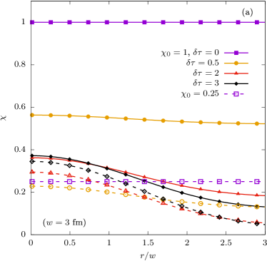
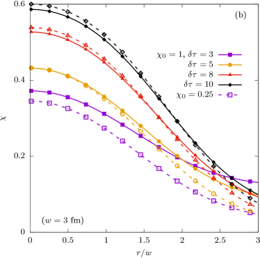
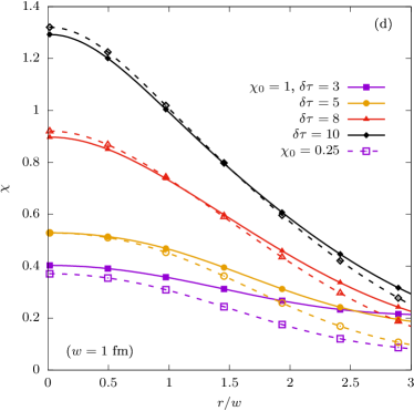
Figure 5: Radial profiles of $\chi$ at different values of $\delta\tau=(\tau-\tau_{0})/\tau_{0}$ for $w=3\ {\rm fm}$ (left column) and $1\ {\rm fm}$ (right column). The initial conditions are $\tau_{0}=0.2\ {\rm fm}$ and $T_{0}=0.5\ {\rm GeV}$, while $\chi_{0}=1$ for the solid curves with filled symbols and $\chi_{0}=0.25$ for the dotted curves with empty symbols. The ratio $\eta/s$ is $0.2$.

Note however that the hydrodynamization occurs at different times for different radii: hydrodynamization in the central region starts earlier than in the intermediate region, and the latest in the outmost region, as we will discuss in more detail below.

As an additional remark for the situation of both the small and the large systems, but more significantly for the smaller system, in the outer regions the hydrodynamization occurs at stages when the energy density has already dropped below values of $1\,{\rm GeV/fm}^{3}$. This behavior might challenge the hydrodynamical simulations of $p+p$ or $p+A$ collisions.

In order to gain more insight on the radial dependence of $\chi$, Fig. 5 shows the radial profiles of $\chi$ at various values of $\tau$, corresponding to the initial conditions $\chi_{0}=1$ (solid lines) and $\chi_{0}=0.25$ (dashed lines). The left and right columns show the $w=3\ {\rm fm}$ and $w=1\ {\rm fm}$ systems, respectively. The top line [panels (a) and (c)] represent the early time evolution of $\chi$. It can be seen that at small times, the evolution of $\chi$ is similar between the $w=3$ and $1\ {\rm fm}$ simulations. At $\delta\tau=(\tau-\tau_{0})/\tau_{0}=3$, it can be seen that the $\chi_{0}=1$ and $\chi_{0}=0.25$ curves are very close to each other around $r=0$. However, the distance between these curves increases with $r$, indicating that hydrodynamization is more rapid at the fireball center than at the system periphery. On the lower line of Fig. 5, the same hydrodynamization can be seen to be achieved at increasingly large $r$ as $\delta\tau$ is increased. This is in line with the analysis of the $0+1{\rm D}$ system from Sec. II, since the hydrodynamization time $\delta\tau_{H}$ is expected to increase due to the increase of the local value of $\tilde{w}_{0}^{-1}(r)=(4\pi\eta/s)/[\tau_{0}T_{0}(r)]$. A key difference between the larger ($w=3\ {\rm fm}$) and smaller ($w=1\ {\rm fm}$) systems is that $\chi$ increases much faster in the latter case. This is because the transverse expansion is driven by larger gradients, becoming dominant compared to the longitudinal expansion at a faster rate than in the larger system.

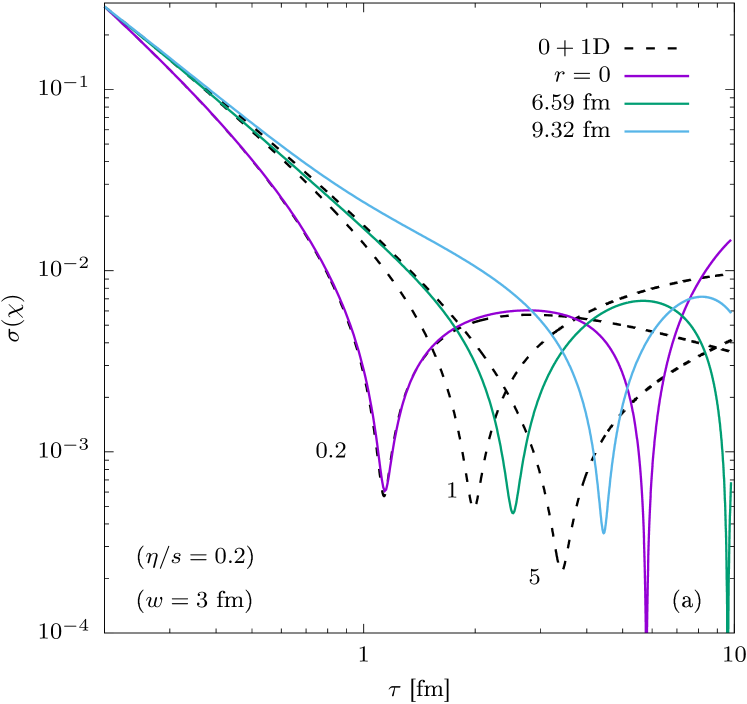
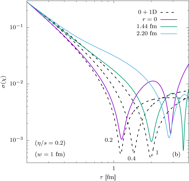
Figure 6: Evolution of $\sigma(\chi)$ measured at various values of $r$ for transversely expanding systems with $\eta/s=0.2$, having widths (a) $w=3\ {\rm fm}$ and (b) $w=1\ {\rm fm}$. The values of $r$ are chosen such that $\tilde{w}_{0}^{-1}(r)=(4\pi\eta/s)/[\tau_{0}T_{0}(r)]$ matches that of the $0+1{\rm D}$ system with $T_{0}=0.5\ {\rm GeV}$ and the values of $\eta/s$ inscribed next to the $0+1{\rm D}$ lines (shown with dotted black lines). The initial time is $\tau_{0}=0.2\ {\rm fm}$.

Focusing now on the systems with $\eta/s=0.2$, we investigate the evolution of $\sigma(\chi)$ at various distances $r$ from the fireball center in Fig. 6. In the $w=3\ {\rm fm}$ system, shown in panel (a), $r=0$ corresponds to the fireball center, while $r=6.59\ {\rm fm}$ and $9.32\ {\rm fm}$ correspond to initial values of the local temperature $T_{0}(r)=0.1$ and $0.02\ {\rm GeV}$, respectively. In the $w=1\ {\rm fm}$ system, the values $1.44\ {\rm fm}$ and $2.20\ {\rm fm}$ of $r$ correspond to $T_{0}(r)=0.25\ {\rm GeV}$ and $0.1\ {\rm GeV}$. The black dotted lines represent results obtained in the $0+1{\rm D}$ system, initialized such that the values of $\tilde{w}_{0}^{-1}=(4\pi\eta/s)/\tau_{0}T_{0}$ match those of the points considered in the transversely expanding systems. In particular, we kept $\tau_{0}=0.2\ {\rm fm}$ and $T_{0}=0.5\ {\rm GeV}$ fixed and considered $\eta/s=0.2$, $1$ and $5$ for $w=3\ {\rm fm}$, while the values $\eta/s=0.2$, $0.4$ and $1$ were employed for the $w=1\ {\rm fm}$ system.

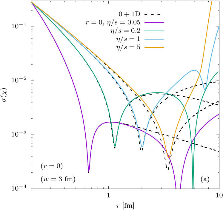
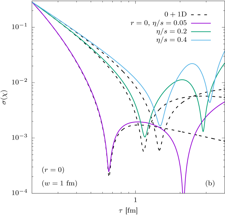
Figure 7: Evolution of $\sigma(\chi)$ measured at $r=0$ for transversely expanding systems with various values of $\eta/s$, having widths (a) $w=3\ {\rm fm}$ and (b) $w=1\ {\rm fm}$. The dotted lines represent results from the $0+1{\rm D}$ system having $T_{0}=0.5\ {\rm GeV}$ and the same value of $\eta/s$ as that in the transversely expanding system. The initial time is $\tau_{0}=0.2\ {\rm fm}$.

As in the $0+1{\rm D}$ system, $\sigma(\chi)$ exhibits a decrease toward a minimum value $\sigma_{\rm min}$ reached after a relatively short time. At $r=0$, the approach to this minimum is almost identical in the $1+1{\rm D}$ system as in the $0+1{\rm D}$ system. As $r$ is increased, the agreement deteriorates and the minimum is reached at a later time. The effect is more pronounced for the smaller system, where the transverse gradients are stronger, which indicates that the effect of the transverse expansion is to delay hydrodynamization in comparison to the prediction of the $0+1{\rm D}$ model.

A remarkable feature seen for the $r=0$ curve in panel (a) of Fig. 6 is that a second minimum emerges at later times, namely at $\tau=5.78\ {\rm fm}$ and $2.50\ {\rm fm}$ for the $w=3\ {\rm fm}$ and $1\ {\rm fm}$ systems, respectively. From Fig. 4, it can be seen that at these times, ${\bar{\chi}}$ is around $1.18$ and $1.58$ for the larger and smaller system, respectively, thus the system evolution at this stage is dominated by the transverse dynamics. Thus, the second minima seen in Fig. 6 reveals a new attractor solution which is due to the transverse expansion of the system.

We now focus on the dynamics at the center of the fireball and consider systems with various values of $\eta/s$. A comparison between the $1+1{\rm D}$ and the corresponding $0+1{\rm D}$ systems is presented in Fig. 7. For the larger system ($w=3\ {\rm fm}$), shown in panel (a), good agreement can be seen even at $\eta/s=5$. In the smaller system, a discrepancy can be seen at the level of the value of $\sigma_{\rm min}$, which increases at larger $\eta/s$. However, for $\eta/s\lesssim 0.4$, the hydrodynamization time $\delta\tau_{H}^{\sigma_{\rm th}=0}$ (when $\sigma$ reaches the local minimum $\sigma_{\rm min}$) remains similar to that of the $0+1{\rm D}$ system. We can thus conclude that the approach to the attractor solution is dominated for both large and small systems by the longitudinal dynamics of the $0+1{\rm D}$ system. For the larger system, the analogy holds up to very high values of $\eta/s$, while the smaller system exhibits more visible deviations even at small $\eta/s$. It is notable that the second minima emerges significantly faster in the smaller system than in the larger system, indicating that hydrodynamization due to transverse expansion is more effective here.

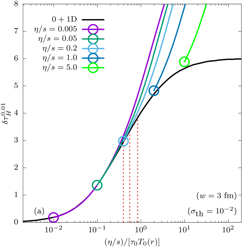
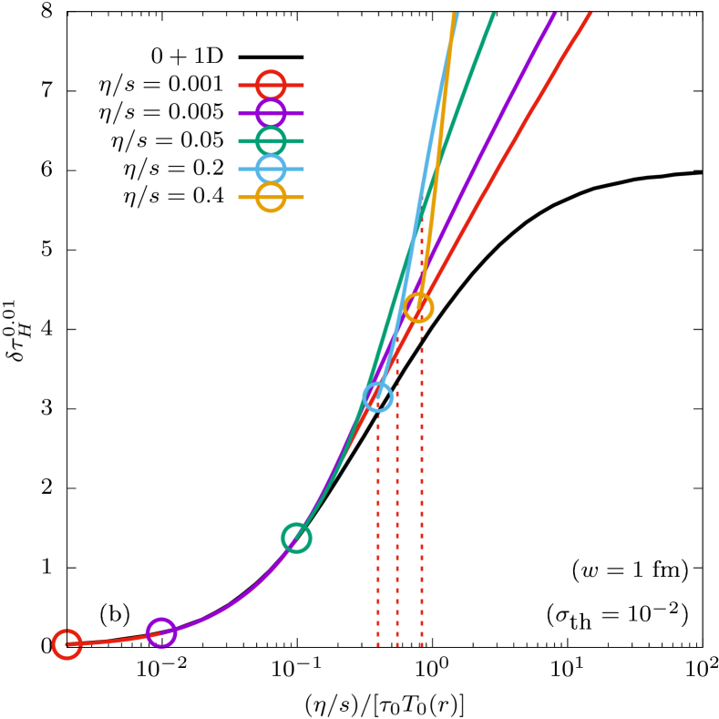
Figure 8: The hydrodynamization timescale $\delta\tau^{0.01}_{H}$ corresponding to a threshold $\sigma_{\rm th}=0.01$ for the $w=3\ {\rm fm}$ (a) and $w=1\ {\rm fm}$ (b) systems, represented with respect to $(\eta/s)/[\tau_{0}T_{0}(r)]$, where the initial temperature $T_{0}(r)$ is given by Eq. (48). The circles represent $\delta\tau^{0.01}_{H}$ corresponding to the central point ($r=0$) of the fireball and each curve corresponds to a different value of $\eta/s$. The red dashed lines mark the positions $r=0$, $w$ and $3w/2$ for the system with $\eta/s=0.2$, corresponding to the curves shown in Fig. 4.

Figure 8 shows the hydrodynamization timescale $\delta\tau^{0.01}_{H}$ (corresponding to $\sigma_{\rm th}=0.01$) in the scenario with transverse expansion achieved from the RTA approach as a function of $\tilde{w}_{0}^{-1}(r)=(4\pi\eta/s)/[\tau_{0}T_{0}(r)]$. The results for the larger ($w=3\ {\rm fm}$) and smaller ($w=1\ {\rm fm}$) systems are shown in panels (a) and (b), respectively. The initial temperature $T_{0}(r)$ decreases with increasing $r$, as indicated in Eq. (48). We considered simulations with $\eta/s$ between $0.001$ and $5$. For each value of $\eta/s$, the simulation covers the $x$-axis range from $\tilde{w}_{0}^{-1}(0)=(4\pi\eta/s)/[\tau_{0}T_{0}(0)]$ up to infinity. It can be seen that $\delta\tau_{H}^{0.01}$ for the $1+1{\rm D}$ system is very similar to that for the $0+1{\rm D}$ system at small values of $\tilde{w}_{0}^{-1}(r)$.

For fixed $\eta/s$, larger deviations between the $0+1{\rm D}$ and $1+1{\rm D}$ results appear as either $r$ is increased or $w$ is decreased. When $\delta\tau_{H}^{0.01}$ for a given point in the system exceeds a certain threshold value ($\delta\tau_{H}\gtrsim 3$ and $2$ for $w=3$ and $1\ {\rm fm}$, respectively), a deviation with respect to the $0+1{\rm D}$ results toward higher values of $\delta\tau_{H}$ can be seen. Furthermore, there are always points which are sufficiently far from the origin to exhibit deviations from the $0+1{\rm D}$ prediction in their hydrodynamization timescale.

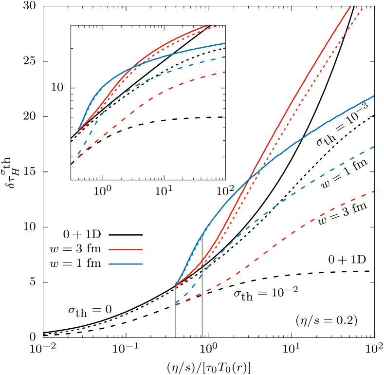
Figure 9: Hydrodynamization time $\delta\tau_{H}^{\sigma_{\rm th}}$ with respect to $(\eta/s)/[\tau_{0}T_{0}(r)]$ for the $w=3\ {\rm fm}$ (red lines) and $1\ {\rm fm}$ (blue lines) systems at $\eta/s=0.2$. The results for $\sigma_{\rm th}=0.01$, $0.001$ and $0$ (corresponding to $\sigma_{\rm min}$) are shown with dashed, dotted and continuous lines, respectively. The black lines represent the $0+1{\rm D}$ results from Fig. 3(b). The gray lines delimit the region between the fireball center and $r=3w/2$. The inset shows the same plot in log-log scale.

We now consider the dependence of $\delta\tau_{H}^{\sigma_{\rm th}}$ on the threshold value $\sigma_{\rm th}$, represented in Fig. 9. As already seen in Fig. 3(b), decreasing $\sigma_{\rm th}$ causes $\delta\tau_{H}^{\sigma_{\rm th}}$ to increase toward the $\delta\tau_{H}^{\sigma_{\rm th}=0}$ limit, achieved when $\sigma_{\rm th}<\sigma_{\rm min}$ (more details regarding this notation are given in Sec. III.1). The analysis focuses on the $\eta/s=0.2$ system, for which $95\%$ of the initial fireball energy (contained within $r\lesssim 1.5w$) is between $0.4\lesssim(\eta/s)/[\tau_{0}T_{0}(r)]\lesssim 0.84$, indicated as gray lines in the figure. In this region, it can be seen that $\delta\tau_{H}^{\sigma_{\rm th}}$ for the larger system behaves essentially as predicted by the $0+1{\rm D}$ system. For the smaller system, $\delta\tau_{H}^{\sigma_{\rm th}}$ is close to the $0+1{\rm D}$ prediction at the fireball center, increasing to a value about $50\%$ larger than the $0+1{\rm D}$ prediction at $r=3w/2$.

For both the larger and the smaller systems, $\delta\tau_{H}^{\sigma_{\rm th}}$ at $\sigma_{\rm th}=10^{-3}$ is almost equal to its limit value $\delta\tau_{H}^{0}$, being further from this limit for the larger system than for the smaller system (for the latter, the curves corresponding to $\sigma_{\rm th}=0.001$ and $0$ are almost overlapped). This indicates that $\sigma_{\rm min}$ has a larger value for the $w=1\ {\rm fm}$ system compared to that for $w=3\ {\rm fm}$, as also seen in Figs. 6 and 7. Furthermore, while for $\sigma_{\rm th}=0.01$, the $w=1\ {\rm fm}$ value for $\delta\tau_{H}^{\sigma_{\rm th}}$ is larger than the value corresponding to $w=3\ {\rm fm}$ over the whole domain considered in Fig. 9, at $\sigma_{\rm th}=0$ it can be seen that $\delta\tau_{H}^{0}$ becomes smaller for $w=1\ {\rm fm}$ when $r\simeq 2.51w$. The time coordinate corresponding to this point, where $\delta\tau_{H}^{0}\simeq 14.45$, is $\tau\simeq 3.09\ {\rm fm}$. As seen in Fig. 4, for the smaller system, the transverse expansion is already dominant, which may explain why hydrodynamization is accelerated compared to the larger system, which is still in a transition phase from longitudinally dominated to transversally dominated expansion.

V Conclusion

In this work, we considered the problem of hydrodynamization in a system of a conformal ideal gas of ultrarelativistic particles undergoing boost-invariant longitudinal expansion with and without transverse dynamics. Quantitatively, we described hydrodynamization on the basis of a (nondimensional) timescale $\delta\tau^{\sigma_{\rm th}}_{H}=(\tau_{H}^{\sigma_{\rm th}}-\tau_{0})/\tau_{0}$, defined in terms of the time $\tau^{\sigma_{\rm th}}_{H}$ in which the standard deviation $\sigma(\chi)$ of the ratio $\chi=\mathcal{P}_{L}/\mathcal{P}_{T}$ with respect to its initial value ($0\leq\chi_{0}\leq 1$ were considered) either reaches its minimum value $\sigma_{\rm min}$, corresponding to the (imperfect) merger of this family of curves, or decreases below a threshold value $\sigma_{\rm th}$.

In the conformal limit of the $0+1{\rm D}$ problem, $\delta\tau^{\sigma_{\rm th}}_{H}$ is a function only of the conformal parameter $\tilde{w}_{0}^{-1}=(4\pi\eta/s)/(\tau_{0}T_{0})$. With respect to this parameter, $\delta\tau^{0.01}_{H}$ (obtained for $\sigma_{\rm th}=0.01$) is bounded between two limits, $\delta\tau_{H}^{0.01}(0)=0$ and $\delta\tau_{H}^{0.01}(\infty)\simeq 6$ (about $1.2\ {\rm fm}$ after initial time $\tau_{0}=0.2\ {\rm fm}$), corresponding to the inviscid and free-streaming regimes, respectively. For the system with transverse dynamics, there appears a competition between the $0+1{\rm D}$ hydrodynamization timescale and the timescale associated with transverse dynamics.

In the $1+1{\rm D}$ setup, we described the initial transverse distribution of Gaussian form with widths $w=1$ and $3\ {\rm fm}$, corresponding to small ($p+p$) and large ($A+A$) collisions. A comparison between the results obtained with the three numerical schemes considered in this paper (Hydro, RTA and BAMPS) is presented in Fig. 4. While Hydro presents some deviations from RTA and BAMPS, the RTA results follow closely the BAMPS results in all tested flow regimes (see Figs. 1, 4, and 10). It is worth stressing that the excellent agreement between RTA and BAMPS recommends RTA as a simulation tool for this type of systems, since it is a significantly faster numerical method than BAMPS.

For the points with sufficiently small values of $(\eta/s)/[\tau_{0}T_{0}(r)]$ (where $T_{0}(r)$ is the local initial temperature), the hydrodynamization time is very well approximated by the $0+1{\rm D}$ prediction. With increasing values of the radius, $\delta\tau_{H}^{\sigma_{\rm th}}$ deviates from the $0+1{\rm D}$ prediction to larger values, faster for the smaller system than for the larger one. For the system with larger transverse size ($w=3\ {\rm fm}$), we found that at $\eta/s=0.2$, the hydrodynamization of the region $r<3w/2$ (containing $95\%$ of the initial energy of the fireball) follows very closely the $0+1{\rm D}$ dynamics. While the center of the smaller fireball is also well captured by the $0+1{\rm D}$ dynamics, hydrodynamization times of up to $50\%$ larger can be seen around $r=3w/2$, indicating that the transverse dynamics has the effect of slowing down hydrodynamization due to longitudinal expansion. Our analysis revealed the emergence of a second minimum of $\sigma(\chi)$, suggesting the existence of an attractor due to the transverse expansion.

In our picture of a heavy-ion collision, our results indicate that for a given $\eta/s$ one always finds a radius in the overlap region beyond which the transversal dynamics become dominant and the hydrodynamization is delayed compared to the innermost region of the fireball. For the outermost regions, this has to be confronted also with the timescales connected with the decrease of energy density and freeze out, making the situation challenging for a hydrodynamical description in the case of very small systems.

Appendix A $0+1{\rm D}$ BJORKEN FLOW FOR HARD-SPHERES

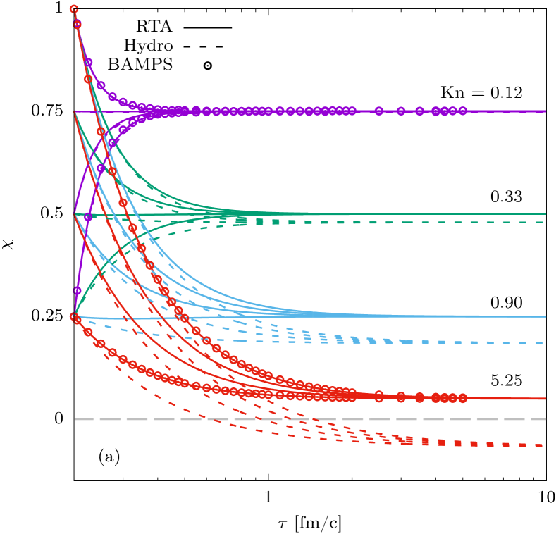
Figure 10: Evolution of the pressure anisotropy $\chi=\mathcal{P}_{L}/\mathcal{P}_{T}$ with respect to the Bjorken time $\tau$ in the context of the hard-sphere gas for various values of the Knudsen number ${\rm Kn}$ (49). The initial conditions are $\tau_{0}=0.2\ {\rm fm}$ and $T_{0}=0.5\ {\rm GeV}$. The RTA and hydro results are shown with solid and dashed lines, respectively, while the BAMPS results are shown using empty circles.

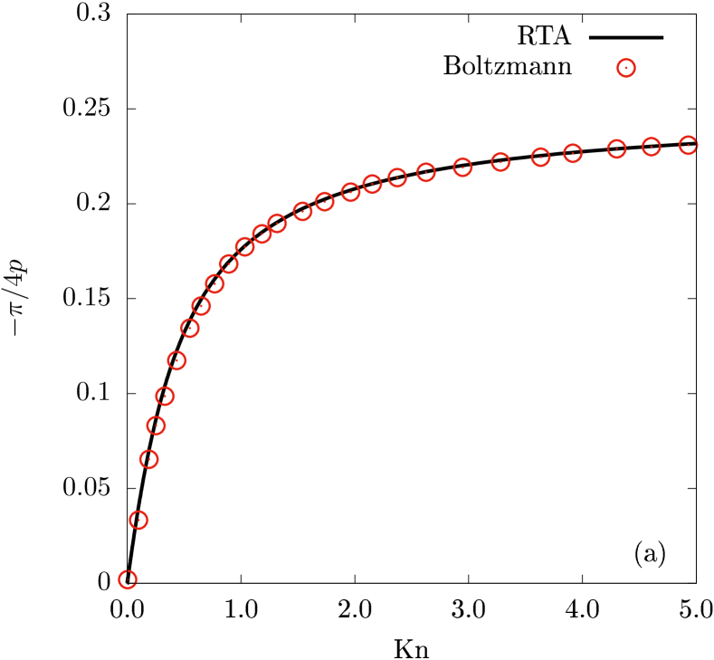
Figure 11: The asymptotic value of $-\pi/4p=(1-\chi)/[2(2+\chi)]$ as a function of the Knudsen number ${\rm Kn}$ (49). Our results obtained using RTA are shown with the black line, while the results reported by Denicol and Noronha [7] are shown with red circles.

In this section, we consider the $0+1{\rm D}$ Bjorken flow of a gas of hard spheres (HS), as described, e.g., by Denicol and Noronha in Ref. [7]. In the context of the BAMPS approach, the collision cross section is set to a constant value $\sigma$. The degree of rarefaction can be conveniently characterized by the Knudsen number ${\rm Kn}$, defined as [7]

$${\rm Kn}=\frac{1}{n\tau\sigma}=\frac{1}{n_{0}\tau_{0}\sigma}.$$ (49)

In the Hydro setup, the HS gas can be implemented by noting that the shear viscosity is related to $\sigma$ via [44]

$$\eta=\frac{1.2654T}{\sigma},$$ (50)

where $T=p/n=p\tau/n_{0}\tau_{0}$ is the local temperature. In the RTA approach, the HS gas is simulated by setting the relaxation time $\tau_{R}$ according to Eq. (6), with $\eta$ given by Eq. (50).

In Fig. 10, the Hydro, RTA, and BAMPS results for $\chi=\mathcal{P}_{L}/\mathcal{P}_{T}$ are compared for various values of ${\rm Kn}$. The initial conditions are set as in Fig. 1, namely $\tau_{0}=0.2\ {\rm fm}$ and $T_{0}=0.5\ {\rm GeV}$. The values of ${\rm Kn}$ are chosen such that the asymptotic value of $\chi$ is $0.75$, $0.5$, $0.25$ and $0.05$. As also noted for the case of the gas with constant $\eta/s$ reported in Fig. 1, all three methods agree at small ${\rm Kn}$. The hydro results exhibit a departure from the RTA and BAMPS results already at ${\rm Kn}=0.33$, achieving negative values for $\chi$ when ${\rm Kn}=5.25$. The agreement between RTA and BAMPS remains excellent for both small and large values of ${\rm Kn}$.

As remarked in Ref. [44] and confirmed in Fig. 10, $\chi$ reaches a constant value as $\tau\rightarrow\infty$, which depends on ${\rm Kn}$. In Fig. 11, we compare our RTA results for $-\Pi/4p=(1-\chi)/[2(2+\chi)]$ with the results computed on the basis of the full Boltzmann collision integral for the hard sphere gas in Ref. [44], finding excellent agreement throughout the whole Knudsen range (between $0$ and $5$).

Appendix B NUMERICAL METHOD FOR THE RTA

In this section, we present the details of the numerical method employed to solve the relativistic Boltzmann equation in the Anderson-Witting relaxation time approximation [26, 27]. The method is inspired by the finite difference Lattice Boltzmann (LB) algorithm [23, 45, 24, 46, 25, 47].

The strategy for devising the numerical method is split into three main parts described in this appendix. The derivation of the relativistic Boltzmann equation in the context of the longitudinal boost-invariant system with transverse expansion is presented in Sec. B.1. At the heart of this derivation is the vielbein formalism [48], which allows spherical coordinates to be employed in the momentum space together with curvilinear spatial coordinates [24].

The momentum space discretization is based on Gauss quadratures for the integration with respect to spherical coordinates and follows LB methodology [45, 23, 24], being described in Sec. B.2. The algorithm for computing the derivatives with respect to the momentum space degrees of freedom, appearing due to the use of a curvilinear coordinate system, is also discussed here.

The spatial and temporal discretization, as well as the numerical schemes employed for the advection and time stepping, are briefly summarized in Sec. B.3.

$w$ (${\rm fm}$)	$\eta/s$	$S$	$\delta\tau/\tau_{0}$	$Q_{\varphi}$	$Q_{\xi}$
$1$	$\leq 0.005$	$200$	$0.005$	$20$	$80$
$1$	$>0.005$	$200$	$0.0025$	$80$	$160$
$3$	(all values)	$200$	$0.01$	$40$	$160$

Table 1: Parameters used for the RTA simulations presented in Sec. IV. See Appendix B for the intepretation of the above notation.

The parameters employed for the simulations discussed in Sec. IV are summarized for convenience in Table 1. We tested that the simulation results were within $1\%$ errors compared to the values obtained by doubling the resolution in any of the numerical parameters shown in Table 1.

B.1 Separation of variables in momentum space using the vielbein formalism

The relativistic Boltzmann equation can be written with respect to the Minkowski (Cartesian) coordinates $(t,x,y,z)$ as follows:

$$k^{\mu}\partial_{\mu}f=C[f],$$ (51)

where $k^{\mu}=(k^{t},k^{x},k^{y},k^{z})$ represent the Cartesian momentum-space components and $C[f]$ is the collision integral (discussed below).

In a system with longitudinal boost invariance, it is convenient to employ the Bjorken coordinates in Eq. (1). Moreover, in this paper, we consider systems with azimuthal symmetry in the transverse plane. Thus, the macroscopic observables depend only on Bjorken time $\tau$ and on the radial distance $r$. The line element (1) becomes

$${\mathrm{d}}s^{2}={\mathrm{d}}\tau^{2}-{\mathrm{d}}r^{2}-r^{2}{\mathrm{d}}\theta^{2}-\tau^{2}{\mathrm{d}}\eta_{s}^{2}.$$ (52)

In order to take advantage of this symmetry in the full phase-space, the momentum space degrees of freedom can be chosen with respect to the following vielbein field (tetrad),

$$e_{\hat{\tau}}= \partial_{\tau}, e_{\hat{r}}= \partial_{r}, e_{\hat{\theta}}= r^{-1}\partial_{\theta}, e_{{\hat{\eta}}_{s}}= \tau^{-1}\partial_{\eta_{s}},$$

$$\omega^{\hat{\tau}}= d\tau, \omega^{\hat{r}}= dr, \omega^{\hat{\theta}}= rd\theta, \omega^{{\hat{\eta}}_{s}}= \tau d\eta_{s}.$$ (53)

The tetrad components $k^{\hat{\alpha}}=k^{\mu}\omega^{\hat{\alpha}}_{\mu}$ are then employed to perform the momentum space integration, such that the particle four-flow vector $N^{\hat{\alpha}}$ and the stress-energy tensor $T^{{\hat{\alpha}}{\hat{\beta}}}$ are computed as follows:

$$N^{\hat{\alpha}}= \int\frac{{\mathrm{d}}^{3}k}{k^{\hat{\tau}}}f\,k^{\hat{\alpha}}, T^{{\hat{\alpha}}\beta}= \int\frac{{\mathrm{d}}^{3}k}{k^{\hat{\tau}}}f\,k^{\hat{\alpha}}k^{\hat{\beta}}.$$ (54)

The hatted indices are raised and lowered with the Minkowski metric $\eta^{{\hat{\alpha}}{\hat{\beta}}}={\rm diag}(1,-1,-1,-1)$, i.e. $N^{\hat{\alpha}}=\eta^{{\hat{\alpha}}{\hat{\beta}}}N_{\hat{\beta}}$. In order to perform the integrals in Eq. (54), it is convenient to introduce spherical coordinates in the momentum space, via

$$\begin{pmatrix}k^{\hat{r}}\\ k^{\hat{\theta}}\end{pmatrix}=k\sqrt{1-\xi^{2}}\begin{pmatrix}\cos\varphi\\ \sin\varphi\end{pmatrix},\qquad k^{{\hat{\eta}}_{s}}=k\xi.$$ (55)

In the case of the ultrarelativistic gas, $k^{\hat{\tau}}=k$.

We are now ready to write down the relativistic Boltzmann equation for the distribution function $f(x^{\mu},k^{\widetilde{\imath}})$ with the phase-space dependence on the curvilinear coordinates $x^{\mu}=(\tau,r,\theta,\eta_{s})$ and the momentum space degrees of freedom $k^{\widetilde{\imath}}=(k,\xi,\varphi)$. It is based on the general theory developed by Cardall and Mezzacappa [48] and employed also in Ref. [24]:

$$\frac{1}{\sqrt{-g}}\partial_{\mu}(\sqrt{-g}e^{\mu}_{\hat{\alpha}}k^{\hat{\alpha}}f)-\frac{k^{\hat{\tau}}}{\sqrt{\lambda}}\frac{\partial}{\partial k^{\widetilde{\imath}}}\left(K^{\widetilde{\imath}}{}_{\hat{\imath}}\Gamma^{\hat{\imath}}{}_{{\hat{\alpha}}{\hat{\beta}}}\frac{k^{\hat{\alpha}}k^{\hat{\beta}}}{k^{\hat{\tau}}}f\sqrt{\lambda}\right)\\ =C[f],$$ (56)

where $\lambda^{-1/2}=|{\rm det}K^{\widetilde{\jmath}}{}_{\hat{\imath}}|$ and the matrix $K^{\widetilde{\jmath}}{}_{{\hat{\imath}}}=\partial k^{\widetilde{\jmath}}/\partial k^{\hat{\imath}}$, computed in Eq. (2.20) of Ref. [24], is reproduced below for convenience:

$$K^{\widetilde{\jmath}}{}_{{\hat{\imath}}}=\begin{pmatrix}\cos\varphi\sqrt{1-\xi^{2}}&\sin\varphi\sqrt{1-\xi^{2}}&\xi\\ -\frac{\xi}{k}\cos\varphi\sqrt{1-\xi^{2}}&-\frac{\xi}{k}\sin\varphi\sqrt{1-\xi^{2}}&\frac{1-\xi^{2}}{k}\\ -\frac{\sin\varphi}{k\sqrt{1-\xi^{2}}}&\frac{\cos\varphi}{k\sqrt{1-\xi^{2}}}&0\end{pmatrix}.$$ (57)

The connection coefficients $\Gamma^{\hat{\imath}}{}_{{\hat{\alpha}}{\hat{\beta}}}$ appearing in Eq. (56) can be computed via

$$\Gamma^{\hat{\sigma}}{}_{{\hat{\beta}}{\hat{\gamma}}}=\frac{1}{2}\eta^{{\hat{\sigma}}{\hat{\alpha}}}(c_{{\hat{\alpha}}{\hat{\beta}}{\hat{\gamma}}}+c_{{\hat{\alpha}}{\hat{\gamma}}{\hat{\beta}}}-c_{{\hat{\beta}}{\hat{\gamma}}{\hat{\alpha}}}),$$ (58)

where the Cartan coefficients are based on the commutators of the vielbein tetrad vectors, $[e_{\hat{\alpha}},e_{\hat{\beta}}]=c_{{\hat{\alpha}}{\hat{\beta}}}{}^{\hat{\gamma}}e_{\hat{\gamma}}$. Based on Eq. (53), we find $c_{\hat{\tau}\hat{\eta}_{s}\hat{\eta}_{s}}=-c_{\hat{\eta}_{s}\hat{\tau}\hat{\eta}_{s}}=\tau^{-1}$ and $c_{\hat{r}\hat{\theta}\hat{\theta}}=-c_{\hat{\theta}\hat{r}\hat{\theta}}=r^{-1}$, with all other Cartan coefficients vanishing, leading to

$$\Gamma^{\hat{\tau}}{}_{{\hat{\eta}}_{s}{\hat{\eta}}_{s}}=\Gamma^{{\hat{\eta}}_{s}}{}_{{\hat{\tau}}{\hat{\eta}}_{s}}=\tau^{-1},\qquad\Gamma^{\hat{r}}{}_{{\hat{\theta}}{\hat{\theta}}}=-\Gamma^{\hat{\theta}}{}_{{\hat{r}}{\hat{\theta}}}=-r^{-1}.$$ (59)

Plugging now Eqs. (57) and (59) into Eq. (56), we find

$$\frac{1}{\tau}\frac{\partial(f\tau)}{\partial\tau}+\frac{k^{\hat{r}}}{rk^{\hat{\tau}}}\frac{\partial(fr)}{\partial r}+\frac{k^{\hat{\theta}}}{rk^{\hat{\tau}}}\frac{\partial f}{\partial\theta}+\frac{k^{{\hat{\eta}}_{s}}}{\tau k^{\hat{\tau}}}\frac{\partial f}{\partial\eta}\\ -\frac{\xi^{2}}{\tau k^{2}}\frac{\partial(fk^{3})}{\partial k}-\frac{1}{\tau}\frac{\partial[\xi(1-\xi^{2})f]}{\partial\xi}-\frac{k\sqrt{1-\xi^{2}}}{rk^{\hat{\tau}}}\frac{\partial(f\sin\varphi)}{\partial\varphi}\\ =\frac{1}{k^{\hat{\tau}}}C[f].$$ (60)

In the case of massless particles (considered throughout this paper and in what follows), $m=0$ and $k^{\hat{\tau}}=k$.

The collision integral $C[f]$ appearing in Eq. (68) is computed in the Anderson-Witting relaxation time approximation (RTA) [26, 27],

$$C[f]\rightarrow C_{\rm A-W}[f]=-\frac{k\cdot u}{\tau_{\rm R}}[f-f^{\rm(eq)}],$$ (61)

where $\tau_{\rm R}$ is the relaxation time and $f^{\rm(eq)}$ is the local equilibrium distribution function. In this paper, we consider that the equilibrium statistics are described by the Maxwell-Jüttner model for massless particles,

$$f^{\rm(eq)}\rightarrow f^{\rm(eq)}_{\rm M-J}= \frac{g}{(2\pi)^{3}}\exp\left(\frac{\mu-k\cdot u}{T}\right)$$

$$= \frac{n}{8\pi T^{3}}\exp\left(-\frac{k\cdot u}{T}\right),$$ (62)

where $g$ is a degeneracy factor ($g=16$ for the gluonic degrees of freedom), while $\mu$ and $T$ are the local chemical potential and temperature, respectively. The macroscopic velocity $u=u^{\hat{\alpha}}e_{\hat{\alpha}}$ is obtained via the Landau matching condition,

$$T^{\hat{\alpha}}{}_{\hat{\sigma}}u^{\hat{\sigma}}=eu^{\hat{\alpha}},$$ (63)

where the energy density $e=3p$ represents the positive eigenvalue of the stress-energy tensor, $T^{\hat{\alpha}}{}_{\hat{\sigma}}$. The temperature $T=p/n$ is determined using the particle number density $n$, which is computed from the particle four-flow and is related to the chemical potential $\mu$ via

$$n=N^{\hat{\alpha}}u_{\hat{\alpha}}=\frac{gT^{3}}{\pi^{2}}e^{\mu/T}.$$ (64)

Both the stress-energy tensor and the particle four-flow are computed using Eq. (54) from the distribution function $f$.

In the case of the $0+1$D Bjorken flow, there is no dependence on the spatial coordinates $r$, $\theta$ and $\eta_{s}$, while the macroscopic velocity is given by $u^{\hat{\alpha}}=(1,0,0,0)^{T}$ at all times. Since we consider no dependence on the azimuthal coordinate $\varphi$ of the momentum space in the initial Romatschke-Strickland distribution given in Eq. (10), it is clear that $\partial_{\varphi}f=0$ at all times and Eq. (60) reduces after setting $m=0$ and $k^{\hat{\tau}}=k$ to

$$\frac{1}{\tau}\frac{\partial(f\tau)}{\partial\tau}-\frac{\xi^{2}}{\tau k^{2}}\frac{\partial(fk^{3})}{\partial k}-\frac{1}{\tau}\frac{\partial[\xi(1-\xi^{2})f]}{\partial\xi}\\ =-\frac{1}{\tau_{R}}[f-f^{\rm(eq)}].$$ (65)

In the free-streaming limit, $\tau_{R}\rightarrow\infty$ and the solution of Eq. (65) is given at time $\tau>\tau_{0}$ precisely by

$$f_{\rm FS}(\tau;k,\xi)=f_{\rm FS}(\tau_{0};\widetilde{k},\widetilde{\xi}),$$ (66)

where [49]

$$\widetilde{k}=k\sqrt{1-\left(\frac{\tau^{2}}{\tau_{0}^{2}}-1\right)\xi^{2}},\qquad\widetilde{\xi}=\frac{k\xi}{\widetilde{k}}\frac{\tau}{\tau_{0}}.$$ (67)

Assuming that the distribution at initial time $f_{\rm FS}(\tau_{0};k,\xi)$ is given by the Romatschke-Strickland $f_{\rm RS}(\tau_{0};k,\xi)$ distribution in Eq. (10), the free-streaming solution (66) reduces to Eq. (41) in the main text.

In the case with transverse expansion, the longitudinal boost invariance and the invariance under azimuthal plane rotations imply that $\partial_{\theta}f=\partial_{\eta_{s}}f=0$. Restricting the discussion to massless particles, when $k^{\hat{\tau}}=k$, Eq. (51) reduces to

$$\frac{1}{\tau}\frac{\partial(f\tau)}{\partial\tau}+\frac{k^{\hat{r}}}{rk}\frac{\partial(fr)}{\partial r}-\frac{\xi^{2}}{\tau k^{2}}\frac{\partial(fk^{3})}{\partial k}\\ -\frac{1}{\tau}\frac{\partial[\xi(1-\xi^{2})f]}{\partial\xi}-\frac{\sqrt{1-\xi^{2}}}{r}\frac{\partial(f\sin\varphi)}{\partial\varphi}\\ =-\frac{k\cdot u}{k\tau_{R}}[f-f^{\rm(eq)}].$$ (68)

The Landau frame velocity $u^{\hat{\alpha}}=(u^{\hat{\tau}},u^{\hat{r}},0,0)$ and the energy density $e$ are given by the solution of the eigenvalue equation (63) [24],

$$e= \frac{1}{2}\left[T^{{\hat{\tau}}{\hat{\tau}}}-T^{{\hat{r}}{\hat{r}}}+\sqrt{(T^{{\hat{\tau}}{\hat{\tau}}}+T^{{\hat{r}}{\hat{r}}})^{2}-4(T^{{\hat{\tau}}{\hat{r}}})^{2}}\right],$$

$$\frac{u^{\hat{r}}}{u^{\hat{\tau}}}= \frac{T^{{\hat{\tau}}{\hat{r}}}}{e+T^{{\hat{r}}{\hat{r}}}}.$$ (69)

B.2 Momentum space discretization

In this paper, we employ the discretization of the momentum space discussed in Ref. [24]. In this scheme, we employ $Q_{L}\times Q_{\xi}\times Q_{\varphi}$ discrete values for $k$, $\xi$ and $\varphi$, such that $k^{\hat{\alpha}}\rightarrow k_{lji}^{\hat{\alpha}}=k_{l}(1,\sqrt{1-\xi_{j}^{2}}\cos\varphi_{i},\sqrt{1-\xi_{j}^{2}}\sin\varphi_{i},\xi_{j})$. The discrete set of distributions $f_{lji}$ are related to the original distribution function $f(k,\xi,\varphi)$ via [24]

$$f_{lji}=\frac{2\pi}{Q_{\varphi}}T_{0}^{3}e^{{\overline{k}}_{l}}w_{l}^{L}w_{j}^{\xi}f(k_{l},\xi_{j},\varphi_{i}).$$ (70)

The weights $w_{l}^{L}$, $w_{j}^{\xi}$ and $2\pi/Q_{\varphi}$ are computed following the prescription of the Gauss-Laguerre, Gauss-Legendre and Mysovskikh (trigonometric) quadratures, respectively [50].

The values for $k$ are chosen as the roots of the generalized Laguerre polynomials $L_{Q_{L}}^{(2)}({\overline{k}})$ of order $Q_{L}$, where ${\overline{k}}=k/k_{\rm ref}$ and $k_{\rm ref}$ is an arbitrary scale which we set equal to the initial temperature, $k_{\rm ref}=T_{0}$. Two values are chosen ($Q_{L}=2$), ${\overline{k}}_{1}=2$ and ${\overline{k}}_{2}=6$, thus ensuring the exact recovery of the evolution of $N^{\hat{\alpha}}$ and $T^{{\hat{\alpha}}{\hat{\sigma}}}$ (for details, see Ref. [24]). The corresponding weights are $w_{1}^{L}=3/2$ and $w_{2}^{L}=1/2$. The derivative term $k^{-2}\partial(fk^{3})/\partial k$ is projected onto the space of generalized Laguerre polynomials and is truncated at order $Q_{L}$, giving

$$\left[\frac{1}{k^{2}}\frac{\partial(fk^{3})}{\partial k}\right]_{lji}=\sum_{\ell^{\prime}=1}^{Q_{L}}\mathcal{K}^{L}_{l,l^{\prime}}f_{l^{\prime}ji},$$ (71)

where the elements of the $Q_{L}\times Q_{L}$ matrix $\mathcal{K}^{L}_{l,l^{\prime}}$ are given in Eq. (3.51) of Ref. [24]. For $L=2$, $\mathcal{K}^{L}_{l,l^{\prime}}=\frac{1}{6}w_{l}^{L}(3-{\overline{k}}_{l}){\overline{k}}_{l^{\prime}}$, such that $\mathcal{K}^{L}_{1,1^{\prime}}=-\mathcal{K}^{L}_{2,1^{\prime}}=\frac{1}{2}$ and $\mathcal{K}^{L}_{1,2^{\prime}}=-\mathcal{K}^{L}_{2,2^{\prime}}=\frac{3}{2}$, leading to

$$\left[\frac{1}{k^{2}}\frac{\partial(fk^{3})}{\partial k}\right]_{1ji}= \frac{1}{2}f_{1ji}+\frac{3}{2}f_{2ji},$$

$$\left[\frac{1}{k^{2}}\frac{\partial(fk^{3})}{\partial k}\right]_{2ji}= -\frac{1}{2}f_{1ji}-\frac{3}{2}f_{2ji}.$$ (72)

In the case of $\xi$, we employ the Gauss-Legendre quadrature of order $Q_{\xi}$, meaning that the values $\xi_{j}$ ($1\leq j\leq Q_{\xi}$) are the roots of the Legendre polynomial of order $Q_{\xi}$, $P_{Q_{\xi}}(\xi_{j})=0$. Both the roots and the weights $w_{j}^{\xi}$ up to order $Q_{\xi}=1000$ are available as data files in the supplementary material of Ref. [24]. The term $\partial[\xi(1-\xi^{2})f]/\partial\xi$ is computed by projection onto the space of Legendre polynomials,

$$\left[\frac{\partial[\xi(1-\xi^{2})f]}{\partial\xi}\right]_{lji}=\sum_{j^{\prime}=1}^{Q_{\xi}}\mathcal{K}^{P}_{j,j^{\prime}}f_{lj^{\prime}i},$$ (73)

where the $Q_{\xi}\times Q_{\xi}$ elements of the matrix $\mathcal{K}^{P}_{j,j^{\prime}}$ are computed from Eq. (3.54) of Ref. [24], reproduced below for convenience:

$$\mathcal{K}^{P}_{j,j^{\prime}}=w_{j}\sum_{m=1}^{Q_{\xi}-3}\frac{m(m+1)(m+2)}{2(2m+3)}P_{m}(\xi_{j})P_{m+2}(\xi_{j^{\prime}})\\ -w_{j}\sum_{m=1}^{Q_{\xi}-1}\frac{m(m+1)}{2}P_{m}(\xi_{j})\Bigg{[}\frac{(2m+1)P_{m}(\xi_{j^{\prime}})}{(2m-1)(2m+3)}\\ +\frac{m-1}{2m-1}P_{m-2}(\xi_{j^{\prime}})\Bigg{]}.$$ (74)

Finally, the trigonometric angle $\varphi$ is discretized using $Q_{\varphi}$ values, $\varphi_{i}=\varphi_{0}+2\pi(i-1)/Q_{\varphi}$ ($1\leq i\leq Q_{\varphi}$), where the arbitrary offset $\varphi_{0}$ is set to $\varphi_{0}=0$ for definiteness. The derivative term $\partial(f\sin\varphi)/\partial\varphi$ can be computed via

$$\left[\frac{\partial(f\sin\varphi)}{\partial\varphi}\right]_{lji}=\sum_{i^{\prime}=1}^{Q_{\varphi}}\mathcal{K}^{M}_{i,i^{\prime}}f_{l,j,i^{\prime}},$$ (75)

where

$$\mathcal{K}^{M}_{i,i^{\prime}}=\frac{1}{Q_{\varphi}}\sum_{m=0}^{\lfloor Q_{\varphi}/2\rfloor}\{(m+1)\cos[m(\varphi_{i}-\varphi_{i^{\prime}})+\varphi_{i}]\\ -(m-1)\cos[m(\varphi_{i}-\varphi_{i^{\prime}})-\varphi_{i}]\},$$ (76)

where $\lfloor\cdot\rfloor$ is the floor function.

Before ending this subsection, we discuss the strategy employed for computing the initial conditions for $f$, as well as the equilibrium distribution $f^{\rm(eq)}$. Because the momentum magnitude $k$ is discretized using only two values, the direct evaluation of the distribution function at these values suffers from severe accuracy problems when attempting to extract the macroscopic quantities $N^{\hat{\alpha}}$ and $T^{{\hat{\alpha}}{\hat{\beta}}}$. Instead, we employ the strategy of Refs. [23, 24] and consider the projection of $f$ onto the space of Laguerre polynomials:

$$f= \frac{e^{-k/T_{0}}}{T_{0}^{3}}\sum_{\ell=0}^{Q_{L}-1}\frac{\mathcal{F}_{\ell}L_{\ell}^{(2)}(k/T_{0})}{(\ell+1)(\ell+2)},$$

$$\mathcal{F}_{\ell}= \int_{0}^{\infty}{\mathrm{d}}p\,p^{2}\,f\,L_{\ell}^{(2)}(k/T_{0}).$$ (77)

The sum over $\ell$ is truncated at $Q_{L}-1$ in order to facilitate the recovery of the integrals of $f$ following the Gauss-Laguerre quadrature prescription. The initialization of $f$ is performed at the level of the coefficients $\mathcal{F}_{\ell}$, which for the Romatschke-Strickland distribution are given by [35]:

$$\mathcal{F}^{\rm RS}_{0}= \frac{ge^{\alpha_{0}}}{(2\pi)^{3}}\frac{\Lambda_{0}^{3}}{(1+\xi_{0}\xi^{2})^{3/2}},$$

$$3\mathcal{F}^{\rm RS}_{0}-\mathcal{F}^{\rm RS}_{1}= \frac{3ge^{\alpha_{0}}}{(2\pi)^{3}}\frac{\Lambda_{0}^{4}/T_{0}}{(1+\xi_{0}\xi^{2})^{2}}.$$ (78)

After the discretization of the momentum space, the Romatschke-Strickland distribution becomes

$$f^{\rm RS}_{lji}=\frac{ge^{\alpha_{0}}\Lambda_{0}^{3}}{(1+\xi_{0}\xi_{j}^{2})^{3/2}}\frac{w_{l}^{L}w_{j}^{\xi}}{4\pi^{2}Q_{\varphi}}\\ \times\left[4-{\bar{k}}_{l}+\frac{\Lambda_{0}/T_{0}}{\sqrt{1+\xi_{0}\xi_{j}^{2}}}(3-{\bar{k}}_{l})\right].$$ (79)

The Maxwell-Jüttner distribution necessary for the computation of the collision term is obtained by replacing $e^{\alpha_{0}}\rightarrow\pi^{2}n/gT^{3}$, $\Lambda_{0}\rightarrow T$ and $\sqrt{1+\xi_{0}\xi^{2}}\rightarrow u_{\hat{\alpha}}k^{\hat{\alpha}}/k=u^{\hat{\tau}}-k^{\hat{r}}u^{\hat{r}}/k$:

$$f^{\rm{(eq)}}_{lji}=\frac{nw_{l}^{L}w_{j}^{\xi}}{4Q_{\varphi}(u^{\hat{\tau}}-u^{\hat{r}}\sqrt{1-\xi_{j}^{2}}\cos\varphi_{i})^{3}}\\ \times\left[4-{\bar{k}}_{l}+\frac{(3-{\bar{k}}_{l})T/T_{0}}{u^{\hat{\tau}}-u^{\hat{r}}\sqrt{1-\xi_{j}^{2}}\cos\varphi_{i}}\right].$$ (80)

B.3 Finite difference methods

The time stepping is performed using the third-order Runge-Kutta scheme [51, 52]. Writing Eq. (68) as $\partial f/\partial\tau=L[f]$ and considering an equal time step discretization of the time coordinate, $\tau_{n}=\tau_{0}+n\delta\tau$, the value $f_{n+1}$ of the distribution function at time step $n+1$ can be obtained from that at time step $n$ via two intermediate stages:

$$f^{(1)}_{n}= f_{n}+\delta tL[f_{n}],$$

$$f^{(2)}_{n}= \frac{3}{4}f_{n}+\frac{1}{4}f^{(1)}_{n}+\frac{1}{4}\delta tL[f^{(1)}_{n}],$$

$$f_{n+1}= \frac{1}{3}f_{n}+\frac{2}{3}f_{n}^{(2)}+\frac{2}{3}\delta tL[f^{(2)}_{n}].$$ (81)

For the advection along $r$, care must be taken because of the $r^{-1}$ factor appearing in Eq. (68). Following Refs. [53, 54, 55], this factor is absorbed in the derivative, i.e. $r^{-1}\partial(fr)/\partial r=2\partial(fr)/\partial r^{2}$. The discretization of the radial coordinate is performed using $S$ equal intervals of width $\delta r=L/S$ (where $L=6w$ and $w$ is the width of the Gaussian, as discussed in Sec. IV), centered on coordinates $r_{s}=(s-\frac{1}{2})\delta r$, with $1\leq s\leq S$. The derivative term is then computed using a flux-based finite-difference scheme,

$$\left[\frac{1}{r}\frac{\partial(fvr)}{\partial r}\right]_{s}=2\frac{r_{s+\frac{1}{2}}\mathcal{F}_{s+\frac{1}{2}}-r_{s-\frac{1}{2}}\mathcal{F}_{s-\frac{1}{2}}}{r_{s+\frac{1}{2}}^{2}-r_{s-\frac{1}{2}}^{2}},$$ (82)

where $r_{s\pm\frac{1}{2}}=r_{s}\pm\frac{1}{2}\delta r$ and $v=k^{\hat{r}}/k^{\hat{\tau}}\rightarrow\cos\varphi_{i}\sqrt{1-\xi_{j}^{2}}$ is the advection velocity. The fluxes $\mathcal{F}_{s\pm\frac{1}{2}}$ are computed using an upwind-biased approach. For increased stability, we employ the fifth-order weighted essentially nonoscillatory (WENO-5) scheme [56, 57], which is summarized also in Refs. [24, 55]. For brevity, the algorithm is not repeated here. We note that, while the WENO-5 method is of fifth order, the formulation in Eq. (82) gives rise to a second-order algorithm due to the $r_{s\pm\frac{1}{2}}$ factors appearing in the numerator [55].

References

- Bjorken [1983] J. D. Bjorken, Highly Relativistic Nucleus-Nucleus Collisions: The Central Rapidity Region, Phys. Rev. D 27, 140 (1983).
- Romatschke and Romatschke [2007] P. Romatschke and U. Romatschke, Viscosity Information from Relativistic Nuclear Collisions: How Perfect is the Fluid Observed at RHIC?, Phys. Rev. Lett. 99, 172301 (2007), arXiv:0706.1522 [nucl-th] .
- Weller and Romatschke [2017] R. D. Weller and P. Romatschke, One fluid to rule them all: viscous hydrodynamic description of event-by-event central p+p, p+Pb and Pb+Pb collisions at TeV, Phys. Lett. B 774, 351 (2017), arXiv:1701.07145 [nucl-th] .
- Heller and Spalinski [2015] M. P. Heller and M. Spalinski, Hydrodynamics Beyond the Gradient Expansion: Resurgence and Resummation, Phys. Rev. Lett. 115, 072501 (2015), arXiv:1503.07514 [hep-th] .
- Mueller [2000] A. H. Mueller, The Boltzmann equation for gluons at early times after a heavy ion collision, Phys. Lett. B 475, 220 (2000), arXiv:hep-ph/9909388 .
- El et al. [2010] A. El, Z. Xu, and C. Greiner, Third-order relativistic dissipative hydrodynamics, Phys. Rev. C 81, 041901(R) (2010), arXiv:0907.4500 [hep-ph] .
- Denicol and Noronha [2020] G. S. Denicol and J. Noronha, Exact hydrodynamic attractor of an ultrarelativistic gas of hard spheres, Phys. Rev. Lett. 124, 152301 (2020), arXiv:1908.09957 [nucl-th] .
- Heller et al. [2018] M. P. Heller, A. Kurkela, M. Spaliński, and V. Svensson, Hydrodynamization in kinetic theory: Transient modes and the gradient expansion, Phys. Rev. D 97, 091503(R) (2018), arXiv:1609.04803 [nucl-th] .
- Romatschke [2017] P. Romatschke, Relativistic Hydrodynamic Attractors with Broken Symmetries: Non-Conformal and Non-Homogeneous, JHEP 12, 079, arXiv:1710.03234 [hep-th] .
- Behtash et al. [2021] A. Behtash, S. Kamata, M. Martinez, T. Schaefer, and V. Skokov, Transasymptotics and hydrodynamization of the Fokker-Planck equation for gluons, Phys. Rev. D 103, 056010 (2021), arXiv:2011.08235 [hep-ph] .
- Kurkela et al. [2020a] A. Kurkela, W. van der Schee, U. A. Wiedemann, and B. Wu, Early- and Late-Time Behavior of Attractors in Heavy-Ion Collisions, Phys. Rev. Lett. 124, 102301 (2020a), arXiv:1907.08101 [hep-ph] .
- Romatschke [2018] P. Romatschke, Relativistic fluid dynamics far from local equilibrium, Phys. Rev. Lett. 120, 012301 (2018).
- Almaalol et al. [2020] D. Almaalol, A. Kurkela, and M. Strickland, Nonequilibrium Attractor in High-Temperature QCD Plasmas, Phys. Rev. Lett. 125, 122302 (2020), arXiv:2004.05195 [hep-ph] .
- Gubser [2010] S. S. Gubser, Symmetry constraints on generalizations of Bjorken flow, Phys. Rev. D 82, 085027 (2010), arXiv:1006.0006 [hep-th] .
- Behtash et al. [2020] A. Behtash, S. Kamata, M. Martinez, and H. Shi, Global flow structure and exact formal transseries of the Gubser flow in kinetic theory, JHEP 07, 226, arXiv:1911.06406 [hep-th] .
- Dash and Roy [2020] A. Dash and V. Roy, Hydrodynamic attractors for Gubser flow, Phys. Lett. B 806, 135481 (2020), arXiv:2001.10756 [nucl-th] .
- Heller et al. [2020] M. P. Heller, R. Jefferson, M. Spaliński, and V. Svensson, Hydrodynamic attractors in phase space, Phys. Rev. Lett. 125, 132301 (2020), arXiv:2003.07368 [hep-th] .
- Baier et al. [2008] R. Baier, P. Romatschke, D. T. Son, A. O. Starinets, and M. A. Stephanov, Relativistic viscous hydrodynamics, conformal invariance, and holography, JHEP 04, 100, arXiv:0712.2451 [hep-th] .
- Kurkela et al. [2020b] A. Kurkela, S. F. Taghavi, U. A. Wiedemann, and B. Wu, Hydrodynamization in systems with detailed transverse profiles, Phys. Lett. B 10.1016/j.physletb.2020.135901 (2020b), arXiv:2007.06851 [hep-ph] .
- Molnar et al. [2010] E. Molnar, H. Niemi, and D. H. Rischke, Numerical tests of causal relativistic dissipative fluid dynamics, Eur. Phys. J. C 65, 615 (2010), arXiv:0907.2583 [nucl-th] .
- Niemi et al. [2012] H. Niemi, G. S. Denicol, P. Huovinen, E. Molnar, and D. H. Rischke, Influence of a temperature-dependent shear viscosity on the azimuthal asymmetries of transverse momentum spectra in ultrarelativistic heavy-ion collisions, Phys. Rev. C 86, 014909 (2012), arXiv:1203.2452 [nucl-th] .
- Fotakis et al. [2020] J. A. Fotakis, M. Greif, C. Greiner, G. S. Denicol, and H. Niemi, Diffusion processes involving multiple conserved charges: A study from kinetic theory and implications to the fluid-dynamical modeling of heavy ion collisions, Phys. Rev. D 101, 076007 (2020), arXiv:1912.09103 [hep-ph] .
- Romatschke et al. [2011] P. Romatschke, M. Mendoza, and S. Succi, A fully relativistic lattice Boltzmann algorithm, Phys. Rev. C 84, 034903 (2011), arXiv:1106.1093 [nucl-th] .
- Ambru\cbs and Blaga [2018] V. E. Ambru\cbs and R. Blaga, High-order quadrature-based lattice Boltzmann models for the flow of ultrarelativistic rarefied gases, Phys. Rev. C 98, 035201 (2018), arXiv:1612.01287 [physics.flu-dyn] .
- Gabbana et al. [2020] A. Gabbana, D. Simeoni, S. Succi, and R. Tripiccione, Relativistic Lattice Boltzmann Methods: Theory and Applications, Phys. Rept. 863, 1 (2020), arXiv:1909.04502 [hep-lat] .
- Anderson and Witting [1974a] J. Anderson and H. Witting, A relativistic relaxation-time model for the boltzmann equation, Physica 74, 466 (1974a).
- Anderson and Witting [1974b] J. Anderson and H. Witting, Relativistic quantum transport coefficients, Physica 74, 489 (1974b).
- Xu and Greiner [2005] Z. Xu and C. Greiner, Thermalization of gluons in ultrarelativistic heavy ion collisions by including three-body interactions in a parton cascade, Phys. Rev. C 71, 064901 (2005), arXiv:hep-ph/0406278 .
- Xu et al. [2008] Z. Xu, C. Greiner, and H. Stocker, PQCD calculations of elliptic flow and shear viscosity at RHIC, Phys. Rev. Lett. 101, 082302 (2008), arXiv:0711.0961 [nucl-th] .
- Gallmeister et al. [2018] K. Gallmeister, H. Niemi, C. Greiner, and D. H. Rischke, Exploring the applicability of dissipative fluid dynamics to small systems by comparison to the Boltzmann equation, Phys. Rev. C 98, 024912 (2018), arXiv:1804.09512 [nucl-th] .
- Jaiswal [2013a] A. Jaiswal, Relativistic dissipative hydrodynamics from kinetic theory with relaxation time approximation, Phys. Rev. C 87, 051901(R) (2013a), arXiv:1302.6311 [nucl-th] .
- Cercignani and Kremer [2002] C. Cercignani and G. M. Kremer, The relativistic Boltzmann equation: theory and applications. (Birkhäuser Verlag, Basel, Switzerland, 2002).
- Romatschke and Strickland [2003] P. Romatschke and M. Strickland, Collective modes of an anisotropic quark gluon plasma, Phys. Rev. D 68, 036004 (2003), arXiv:hep-ph/0304092 .
- Florkowski et al. [2013] W. Florkowski, R. Ryblewski, and M. Strickland, Testing viscous and anisotropic hydrodynamics in an exactly solvable case, Phys. Rev. C 88, 024903 (2013), arXiv:1305.7234 [nucl-th] .
- Ambru\cbs and Guga-Ro\cbsian [2019] V. E. Ambru\cbs and C. Guga-Ro\cbsian, Lattice Boltzmann study of the one-dimensional boost-invariant expansion with anisotropic initial conditions, AIP Conf. Proc. 2071, 020014 (2019), arXiv:1807.10143 [nucl-th] .
- Jaiswal [2013b] A. Jaiswal, Relativistic third-order dissipative fluid dynamics from kinetic theory, Phys. Rev. C 88, 021903(R) (2013b), arXiv:1305.3480 [nucl-th] .
- Florkowski and Ryblewski [2011] W. Florkowski and R. Ryblewski, Highly-anisotropic and strongly-dissipative hydrodynamics for early stages of relativistic heavy-ion collisions, Phys. Rev. C 83, 034907 (2011), arXiv:1007.0130 [nucl-th] .
- Martinez and Strickland [2010] M. Martinez and M. Strickland, Dissipative Dynamics of Highly Anisotropic Systems, Nucl. Phys. A 848, 183 (2010), arXiv:1007.0889 [nucl-th] .
- Molnár et al. [2016] E. Molnár, H. Niemi, and D. H. Rischke, Closing the equations of motion of anisotropic fluid dynamics by a judicious choice of a moment of the Boltzmann equation, Phys. Rev. D 94, 125003 (2016), arXiv:1606.09019 [nucl-th] .
- Kamata et al. [2020] S. Kamata, M. Martinez, P. Plaschke, S. Ochsenfeld, and S. Schlichting, Hydrodynamization and nonequilibrium Green’s functions in kinetic theory, Phys. Rev. D 102, 056003 (2020), arXiv:2004.06751 [hep-ph] .
- Blaizot and Yan [2021] J.-P. Blaizot and L. Yan, On attractor and fixed points in Bjorken flows, (2021), arXiv:2106.10508 [nucl-th] .
- Schenke et al. [2011] B. Schenke, S. Jeon, and C. Gale, Elliptic and triangular flow in event-by-event (3+1)D viscous hydrodynamics, Phys. Rev. Lett. 106, 042301 (2011), arXiv:1009.3244 [hep-ph] .
- Uphoff et al. [2015] J. Uphoff, F. Senzel, O. Fochler, C. Wesp, Z. Xu, and C. Greiner, Elliptic flow and nuclear modification factor in ultrarelativistic heavy-ion collisions within a partonic transport model, Phys. Rev. Lett. 114, 112301 (2015), arXiv:1401.1364 [hep-ph] .
- Denicol et al. [2012] G. Denicol, H. Niemi, E. Molnar, and D. Rischke, Derivation of transient relativistic fluid dynamics from the Boltzmann equation, Phys. Rev. D 85, 114047 (2012), [Erratum: Phys.Rev.D 91, 039902 (2015)], arXiv:1202.4551 [nucl-th] .
- Ambru\cbs and Sofonea [2012] V. E. Ambru\cbs and V. Sofonea, High-order thermal lattice boltzmann models derived by means of gauss quadrature in the spherical coordinate system, Physical Review E 86, 016708 (2012).
- Succi [2018] S. Succi, The Lattice Boltzmann Equation: For Complex States of Flowing Matter (Oxford Univ. Press, Oxford, UK, 2018).
- Bazzanini et al. [2021] L. Bazzanini, A. Gabbana, D. Simeoni, S. Succi, and R. Tripiccione, A Lattice Boltzmann Method for Relativistic Rarefied Flows in (2 + 1) Dimensions, J. Comput. Sci. 51, 101320 (2021), arXiv:2011.06856 [physics.flu-dyn] .
- Cardall and Mezzacappa [2003] C. Y. Cardall and A. Mezzacappa, Conservative formulations of general relativistic kinetic theory, Phys. Rev. D 68, 023006 (2003), arXiv:astro-ph/0212460 .
- Kurkela et al. [2019] A. Kurkela, U. A. Wiedemann, and B. Wu, Opacity dependence of elliptic flow in kinetic theory, Eur. Phys. J. C 79, 759 (2019), arXiv:1805.04081 [hep-ph] .
- Mysovskikh [2003] I. P. Mysovskikh, Cubature formulae that are exact for trigonometric polynomials, Dokl. Akad. Nauk SSSR 296, 023006 (2003), sov. Math. Dokl. 36, 229 (1988).
- Shu and Osher [1988] C.-W. Shu and S. Osher, Efficient implementation of essentially non-oscillatory shock-capturing schemes, J. Comput. Phys. 77, 439 (1988).
- Gottlieb and Shu [1998] S. Gottlieb and C.-W. Shu, Total variation diminishing Runge-Kutta schemes, Math. Comp. 67, 73 (1998).
- Falle and Komissarov [1996] S. A. E. G. Falle and S. S. Komissarov, An upwind numerical scheme for relativistic hydrodynamics with a general equation of state, Mon. Not. R. Astron. Soc. 278, 586 (1996).
- Downes et al. [2002] T. P. Downes, P. Duffy, and S. S. Komissarov, Relativistic blast waves and synchrotron emission, Mon. Not. R. Astron. Soc. 332, 144 (2002).
- Busuioc and Ambru\cbs [2019] S. Busuioc and V. E. Ambru\cbs, Lattice Boltzmann models based on the vielbein formalism for the simulation of flows in curvilinear geometries, Phys. Rev. E 99, 033304 (2019).
- Jiang and Shu [1996] G. S. Jiang and C. W. Shu, Efficient Implementation of Weighted ENO Schemes, J. Comput. Phys. 126, 202 (1996).
- Rezzolla and Zanotti [2013] L. Rezzolla and O. Zanotti, Relativistic hydrodynamics (Oxford University Press, Oxford, UK, 2013).