Anisotropic active Brownian particle with a fluctuating propulsion force

Abstract

The active Brownian particle (ABP) model describes a swimmer, synthetic or living, whose direction of swimming is a Brownian motion. The swimming is due to a propulsion force, and the fluctuations are typically thermal in origin. We present a 2D model where the fluctuations arise from nonthermal noise in a propelling force acting at a single point, such as that due to a flagellum. We take the overdamped limit and find several modifications to the traditional ABP model. Since the fluctuating force causes a fluctuating torque, the diffusion tensor describing the process has a coupling between translational and rotational degrees of freedom. An anisotropic particle also exhibits a mass-dependent noise-induced drift, which does not disappear in the overdamped limit. We show that these effects have measurable consequences for the long-time diffusivity of active particles, in particular adding a contribution that is independent of where the force acts.

[Note: at the end of the paper is a Nomenclature of mathematical symbols, in the order introduced.]

Modeling swimming microorganisms is a challenge, since biological entities resist a simple, uniform description. Nevertheless we need models to explain physical observations and develop intuition, and the hope is that the models capture some essential aspect of an organism’s behavior. For microswimmers, most modeling efforts impose some randomness to the motion. The simplest approach is to use a fixed propulsion speed, together with a random re-orientation mechanism. The random re-orientation comes in two main flavors: a run-and-tumble process where the organism makes large excursions and changes its orientation sporadically [1, 2, 3, 4, 5, 6, 7], and a Brownian process where the direction of swimming gradually varies [8, 9, 10, 11, 12, 13, 14]. Both of these models have their place, but in this letter we focus primarily on the latter, Brownian approach.

In this letter we present a simple model of random microorganism motion where the swimmer is propelled by a fluctuating force acting at a point (Fig. 1). The randomness is built into the force as a covariance matrix, and is not due to interactions with the medium (though such interactions could be included as well). Our goal is to derive effective equations of motion for this simple configuration, which is meant to represented an organism with a single flagellum. The resulting equations have some points of commonality with the well-known Active Brownian particle model (ABP), but differ in crucial ways. In particular, there is an inherent coupling between translational and rotation diffusivities. In addition, there is a noise-induced drift that is present regardless of which stochastic interpretation (Itô or Stratonovich) is used.

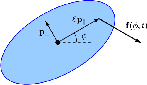
Figure 1: A 2D particle with orientation $\phi$ subject to a time-dependent force $\bm{f}$ acting at a point $\ell\bm{p}_{\parallel}(\phi)$ with respect to its center of reaction.

The stochastic equations (SDEs) for the 2D ABP model are [8, 9, 10, 11, 12, 13, 14]

$$\dot{\bm{x}} =(U+\sqrt{\smash[b]{2D_{\parallel}}}\,\dot{w}_{\parallel})\,\bm{p}_{\parallel}+\sqrt{\smash[b]{2D_{\perp}}}\,\bm{p}_{\perp}\,\dot{w}_{\perp}\,,$$ (1a)

$$\dot{\phi} =\Omega+\sqrt{\smash[b]{2D_{\mathrm{r}}}}\,\dot{w}_{\mathrm{r}}\,.$$ (1b)

The swimmer is moving at constant speed $U$ in the direction $\bm{p}_{\parallel}(\phi)$ and rotating at constant angular speed $\Omega$. The translational noises $\sqrt{\smash[b]{2D_{\parallel}}}\,\dot{w}_{\parallel}$ and $\sqrt{\smash[b]{2D_{\perp}}}\,\dot{w}_{\perp}$ are respectively along ($\bm{p}_{\parallel}$) and perpendicular ($\bm{p}_{\perp}$) to the direction of swimming, and the rotational noise $\sqrt{\smash[b]{2D_{\mathrm{r}}}}\,\dot{w}_{\mathrm{r}}$ affects the swimming direction. The $w_{i}(t)$ are independent standard Wiener processes. Equation 1 has been very successful in modeling the swimming and collective behavior of many microorganisms [15, 16, 17, 18, 19, 20, 21]. The noises are often taken to be due to thermal fluctuations, in which case they satisfy the Einstein–Smoluchowski relations $D_{i}=(\beta\sigma_{i})^{-1}$, for $i\in\{\parallel,\perp,{\mathrm{r}}\}$, where $\sigma_{i}$ are the components of the diagonal grand resistance tensor and $\beta$ is the inverse temperature $1/k_{\mathrm{B}}T$.

In this letter we derive a modified ABP model by assuming that the noise is due to a fluctuating propulsion force acting at a single point on the particle, rather than a thermal bath. We will find several new effects: a new noise-induced drift term, as well as a diffusion matrix that couples the rotational and angular degrees of freedom.

A particle subjected to a fluctuating force $\bm{f}(\phi,t)=(F_{\parallel}+\sqrt{\smash[b]{2E_{\parallel}}}\,\dot{w}_{\parallel})\,\bm{p}_{\parallel}+(F_{\perp}+\sqrt{\smash[b]{2E_{\perp}}}\,\dot{w}_{\perp})\,\bm{p}_{\perp}$ acting at the point $\ell\,\bm{p}_{\parallel}$ with respect to the center of reaction [22] obeys the Langevin equations

$$m\dot{\bm{u}}=-\mathbb{K}\cdot\bm{u}+\bm{f},\quad I\,\dot{\omega}=-\sigma_{\mathrm{r}}\,\omega+\tau,$$ (2)

where $m$ is the mass, $I$ the moment of inertia, $\bm{u}$ the velocity, $\omega$ the angular velocity, and $\mathbb{K}=\mathbb{Q}\cdot\operatorname{diag}(\sigma_{\parallel},\sigma_{\perp})\cdot\mathbb{Q}^{\top}$ the resistance matrix, with $\mathbb{Q}(\phi)$ a $2\times 2$ rotation matrix. The force exerts a torque $\tau(t)=\ell\,(F_{\perp}+\sqrt{\smash[b]{2E_{\perp}}}\,\dot{w}_{\perp})$ .

A brief note on the validity of Eq. 2 is in order. We follow many authors such as [24, 25] and use a linear damping law in Eq. 2, which as first pointed out by Lorentz [26] is strictly only valid in the limit where the fluid density is less than the particle density [27, 28, 29, 30, 31, 32]. The theory could be extended to allow for a memory kernel, the so-called Basset–Boussinesq integral term [33, 34], but then the process is non-Markovian and we cannot recover a simple Fokker–Planck equation as detailed below. Nevertheless, we expect that this memory effect is unlikely to decrease correlations, and so the effects presented here might be modified but would not disappear.

We rewrite the system (2) in the standard form

$$\frac{\mathrm{d}\widehat{\bm{x}}}{\mathrm{d}t}=\widehat{\bm{u}},\quad\frac{\mathrm{d}\widehat{\bm{u}}}{\mathrm{d}t}=\widehat{\mathbb{B}}\cdot(\widehat{\bm{U}}-\widehat{\bm{u}})+\widehat{\mathbb{\Sigma}}\cdot\dot{\bm{w}}$$ (3)

where $\widehat{\bm{x}}=(\bm{x},\phi)$, $\widehat{\bm{u}}=(\bm{u},\omega)$, $\dot{\bm{w}}=(\dot{w}_{\parallel},\dot{w}_{\perp})$, $\widehat{\mathbb{B}}=\operatorname{diag}(\mathbb{K}/m,\sigma_{\mathrm{r}}/I)$, $\widehat{\bm{U}}=(\bm{U},\Omega)=(\mathbb{K}^{-1}\cdot\bm{F},\ell F_{\perp}/\sigma_{\mathrm{r}})$, and

$$\widehat{\mathbb{\Sigma}}=\begin{pmatrix}(\sqrt{\smash[b]{2E_{\parallel}}}/m)\,\bm{p}_{\parallel}&(\sqrt{\smash[b]{2E_{\perp}}}/m)\,\bm{p}_{\perp}\\ 0&\sqrt{\smash[b]{2E_{\perp}}}\,\ell/I\end{pmatrix}.$$ (4)

The third components of hat-wearing vectors and matrices pertain to angular quantities.

Typically, in the overdamped limit (small mass, or large drag) the term $\mathrm{d}\widehat{\bm{u}}/\mathrm{d}t$ in (3) is neglected, resulting in the equation

$$\frac{\mathrm{d}\widehat{\bm{x}}}{\mathrm{d}t}=\widehat{\bm{U}}+\widehat{\mathbb{B}}^{-1}\cdot\widehat{\mathbb{\Sigma}}\cdot\dot{\bm{w}}.$$ (5)

This recovers something close to the standard ABP model (1), except that here there are only two rather than three independent noises: the rotational noise is correlated to the translational noise, since the former is caused by the torque of the latter. We will see the consequences of this correlation below.

But first note that taking the overdamped limit in this way is suspicious. The underdamped equations (3) have the same form independent of the interpretation given to the stochastic product (i.e., Itô or Stratonovich), even though the noise appears multiplicative at first glance. However, the noise coupling matrix $\widehat{\mathbb{B}}^{-1}\cdot\widehat{\mathbb{\Sigma}}$ in Eq. 5 leads to a nonvanishing drift term when the stochastic product is interpreted in the Stratonovich sense [35, p. 83]. This suggests that Eq. 5 has a uniquely-defined noise-induced drift term [36, 37, 38], but the naive way of passing from (3) to (5) does not tell us what form it should take.

A more systematic approach is required to find the missing noise-induced drift term Eq. 5. Instead working with SDEs, we take the overdamped limit of the Fokker–Planck equation for the probability density $p(\widehat{\bm{x}},\widehat{\bm{u}},t)$ corresponding to Eq. 3 (see [36, 39, 40, 41] for an SDE approach):

$$\varepsilon^{2}\,\partial_{t}p+\varepsilon\,\nabla_{\widehat{\bm{x}}}\cdot(\widehat{\bm{u}}\,p)+\varepsilon\,\nabla_{\widehat{\bm{u}}}\cdot(\widehat{\mathbb{B}}\cdot\widehat{\bm{U}}p)=\mathcal{L}p$$ (6)

where $\varepsilon$ is a formal expansion parameter, with $\varepsilon\rightarrow 0$ the overdamped limit, and

$$\mathcal{L}p\mathrel{\raisebox{0.29707pt}{:}\!\!=}\nabla_{\widehat{\bm{u}}}\cdot\bigl{(}\widehat{\mathbb{B}}\cdot\widehat{\bm{u}}\,p\bigr{)}+\nabla_{\widehat{\bm{u}}}\otimes\nabla_{\widehat{\bm{u}}}:\bigl{(}\widehat{\mathbb{{E}}}\,p\bigr{)}$$ (7)

with $\widehat{\mathbb{{E}}}\mathrel{\raisebox{0.29707pt}{:}\!\!=}\tfrac{1}{2}\widehat{\mathbb{\Sigma}}\cdot\widehat{\mathbb{\Sigma}}^{\top}$ . The parameter $\varepsilon$ expresses the long-time and large-scale rescalings of $t$ and $\widehat{\bm{x}}$ for which the $\widehat{\bm{u}}$ degrees of freedom equilibrate.

Now we proceed order-by-order with an expansion $p=p_{0}+\varepsilon\,p_{1}+\cdots$. At leading order we have $\mathcal{L}p_{0}=0$, with solution $p_{0}=P(\widehat{\bm{x}},t)\,\varphi(\widehat{\bm{x}},\widehat{\bm{u}})$, where $P$ is yet to be determined and $\varphi(\widehat{\bm{x}},\widehat{\bm{u}})$ is the invariant density for an Ornstein–Uhlenbeck process [43]:

$$\varphi=(2\pi)^{-3}(\det\widehat{\mathbb{A}})^{-1/2}\,\exp\bigl{(}-\tfrac{1}{2}\,\widehat{\bm{u}}\cdot\widehat{\mathbb{A}}^{-1}\cdot\widehat{\bm{u}}\bigr{)}.$$ (8)

Here the symmetric positive-definite matrix $\widehat{\mathbb{A}}(\widehat{\bm{x}})$ is the unique solution to the continuous-time Lyapunov equation 

$$\widehat{\mathbb{B}}\cdot\widehat{\mathbb{A}}+\widehat{\mathbb{A}}\cdot\widehat{\mathbb{B}}^{\top}=2\widehat{\mathbb{{E}}}$$ (9)

where in our case $\widehat{\mathbb{B}}=\widehat{\mathbb{B}}^{\top}$. When $\widehat{\mathbb{B}}$ commutes with $\widehat{\mathbb{{E}}}$, as occurs for thermal fluctuations, the solution to (9) is $\widehat{\mathbb{A}}=\widehat{\mathbb{{E}}}\cdot\widehat{\mathbb{B}}^{-1}$; this is not the case here, and we find instead

$$\widehat{\mathbb{A}}=\widehat{\mathbb{Q}}\cdot\begin{pmatrix}\frac{E_{\parallel}}{m\sigma_{\parallel}}&0&0\\ 0&\frac{E_{\perp}}{m\sigma_{\perp}}&\frac{2E_{\perp}\ell}{m\sigma_{\mathrm{r}}+I\sigma_{\perp}}\\ 0&\frac{2E_{\perp}\ell}{m\sigma_{\mathrm{r}}+I\sigma_{\perp}}&\frac{E_{\perp}\ell^{2}}{I\sigma_{\mathrm{r}}}\end{pmatrix}\cdot\widehat{\mathbb{Q}}^{\top}$$ (10)

where $\widehat{\mathbb{Q}}(\phi)=\operatorname{diag}(\mathbb{Q},1)$ is a $3\times 3$ rotation matrix about the third axis.

At the next order in $\varepsilon$, we have $\mathcal{L}p_{1}=\nabla_{\widehat{\bm{x}}}\cdot(\widehat{\bm{u}}\,\varphi\,P)-\widehat{\bm{u}}\cdot\widehat{\mathbb{A}}^{-1}\cdot\widehat{\mathbb{B}}\cdot\widehat{\bm{U}}\varphi P$. The solution can be written in two pieces $p_{1}=p_{1}^{(1)}+p_{1}^{(2)}$, with $p_{1}^{(1)}=(\nabla_{\widehat{\bm{x}}}P-\widehat{\bm{U}}\cdot\widehat{\mathbb{B}}^{\top}\cdot\widehat{\mathbb{A}}^{-1}\,P)\cdot\widehat{\bm{\chi}}^{(1)}$ and $p_{1}^{(2)}=-\tfrac{1}{2}P\,\nabla_{\widehat{\bm{x}}}\widehat{\mathbb{A}}^{-1}\,\raisebox{-1.99997pt}{$\vdots$}\,\widehat{\bm{\chi}}^{(2)}$, where $\widehat{\bm{\chi}}^{(1)}$ and $\widehat{\bm{\chi}}^{(2)}$ satisfy

$$\mathcal{L}\widehat{\bm{\chi}}^{(1)}=\widehat{\bm{u}}\,\varphi,\qquad\mathcal{L}\widehat{\bm{\chi}}^{(2)}=\widehat{\bm{u}}\widehat{\bm{u}}\widehat{\bm{u}}\,\varphi.$$ (11)

It is easy to solve for $\widehat{\bm{\chi}}^{(1)}=-\widehat{\mathbb{A}}\cdot\widehat{\mathbb{B}}^{-\top}\cdot\widehat{\mathbb{A}}^{-1}\cdot\widehat{\bm{u}}\,\varphi$; $\widehat{\bm{\chi}}^{(2)}$ is harder to solve for in general. However, we shall not need its precise expression in our derivation.

At the next and final order in $\varepsilon$ we get from Eq. 6 $\mathcal{L}p_{2}=\nabla_{\widehat{\bm{x}}}\cdot(\widehat{\bm{u}}\,p_{1})+\nabla_{\widehat{\bm{u}}}\cdot(\widehat{\mathbb{B}}\cdot\widehat{\bm{U}}p_{1})+\partial_{t}p_{0}$, to which we need only apply a solvability condition by integrating over $\widehat{\bm{u}}$ (denoted by angle brackets):

$$\partial_{t}P=-\nabla_{\widehat{\bm{x}}}\cdot\langle\widehat{\bm{u}}p_{1}\rangle.$$ (12)

To evaluate the average $\langle\widehat{\bm{u}}\,p_{1}\rangle$, first note that the adjoint to $\mathcal{L}$ is

$$\mathcal{L}^{*}g=-\widehat{\bm{u}}\cdot\widehat{\mathbb{B}}^{\top}\cdot\nabla_{\widehat{\bm{u}}}g+\widehat{\mathbb{{E}}}:\nabla_{\widehat{\bm{u}}}\otimes\nabla_{\widehat{\bm{u}}}g$$ (13)

which satisfies $\langle g\mathcal{L}f\rangle=\langle(\mathcal{L}^{*}g)f\rangle$ for functions $f$ and $g$ vanishing as $\lvert\widehat{\bm{u}}\rvert\rightarrow\infty$. Multiplying the $\widehat{\bm{\chi}}^{(1)}$ equation in (11) by $\widehat{\bm{u}}$, we have

$$\langle\widehat{\bm{u}}\,\mathcal{L}\widehat{\bm{\chi}}^{(1)}\rangle=\langle\widehat{\bm{u}}\widehat{\bm{u}}\,\varphi\rangle=\widehat{\mathbb{A}}\,.$$ (14)

But then using the adjoint property in (14) gives

$$\langle(\mathcal{L}^{*}\widehat{\bm{u}})\,\widehat{\bm{\chi}}^{(1)}\rangle=\langle(-\widehat{\mathbb{B}}\cdot\widehat{\bm{u}})\,\widehat{\bm{\chi}}^{(1)}\rangle=-\widehat{\mathbb{B}}\cdot\langle\widehat{\bm{u}}\,\widehat{\bm{\chi}}^{(1)}\rangle$$

from which we obtain $\langle\widehat{\bm{u}}\widehat{\bm{\chi}}^{(1)}\rangle=-\widehat{\mathbb{B}}^{-1}\cdot\widehat{\mathbb{A}}$. We can play a similar trick with the $\widehat{\bm{\chi}}^{(2)}$ equation to obtain $\langle\widehat{\bm{u}}\,\widehat{\bm{\chi}}^{(2)}\rangle=-\widehat{\mathbb{B}}^{-1}\cdot\langle\widehat{\bm{u}}\widehat{\bm{u}}\widehat{\bm{u}}\widehat{\bm{u}}\,\varphi\rangle$, where the fourth moment for the Gaussian $\varphi$ is easily obtained. We have thus evaluated the required average $\langle\widehat{\bm{u}}\,\widehat{\bm{\chi}}^{(2)}\rangle$ without needing to solve for $\widehat{\bm{\chi}}^{(2)}$.

After a lengthy but straightforward calculation we find $\langle\widehat{\bm{u}}p_{1}\rangle=\widehat{\bm{U}}P-\nabla_{\widehat{\bm{x}}}\cdot(\widehat{\mathbb{A}}\,P)\cdot\widehat{\mathbb{B}}^{-\top}$, which we insert back into (12)to finally obtain

$$\partial_{t}P+\nabla_{\widehat{\bm{x}}}\cdot(\widehat{\bm{U}}P)=\nabla_{\widehat{\bm{x}}}\cdot(\nabla_{\widehat{\bm{x}}}\cdot(\widehat{\mathbb{A}}\,P)\cdot\widehat{\mathbb{B}}^{-\top}).$$ (15)

We rewrite (15) in a more convenient form and obtain the first main result of this letter:

$$\partial_{t}P+\nabla_{\bm{x}}\cdot((\bm{U}+\bm{V})P)+\partial_{\phi}(\Omega\,P)\\ =\nabla_{\widehat{\bm{x}}}\otimes\nabla_{\widehat{\bm{x}}}:(\widehat{\mathbb{D}}\,P)$$ (16)

where the noise-induced drift [45, 37, 46, 47, 41, 48, 38] is

$$\bm{V} =\frac{2\ell E_{\perp}(\sigma_{\parallel}^{-1}-\sigma_{\perp}^{-1})}{\sigma_{\mathrm{r}}(1+I\sigma_{\perp}/m\sigma_{\mathrm{r}})}\,\bm{p}_{\parallel}$$ (17)

and the translational-rotational grand diffusion tensor is

$$\widehat{\mathbb{D}}=\widehat{\mathbb{Q}}\cdot\begin{pmatrix}D_{\parallel}&0&0\\ 0&D_{\perp}&\sqrt{D_{\perp}D_{\mathrm{r}}}\\ 0&\sqrt{D_{\perp}D_{\mathrm{r}}}&D_{\mathrm{r}}\end{pmatrix}\cdot\widehat{\mathbb{Q}}^{\top}\,$$ (18)

with $D_{\parallel}=E_{\parallel}/\sigma_{\parallel}^{2}$, $D_{\perp}=E_{\perp}/\sigma_{\perp}^{2}$, and $D_{\mathrm{r}}=E_{\perp}\ell^{2}/\sigma_{\mathrm{r}}^{2}$. The diffusion tensor couples translational and rotational noises. Our result is closely related to [47], but here the induced drift is due to angular dependence rather than spatial inhomogeneity.

To go back and compare to the overdamped result Eq. 5 obtained by simply neglecting the particle mass, the Fokker–Planck equation (16) implies the SDE

$$\frac{\mathrm{d}}{\mathrm{d}t}\begin{pmatrix}\bm{x}\\ \phi\end{pmatrix}=\begin{pmatrix}\bm{U}+\bm{V}\\ \Omega\end{pmatrix}+\sqrt{2\widehat{\mathbb{D}}}\cdot\dot{\bm{w}}$$ (19)

where $\sqrt{2\widehat{\mathbb{D}}}=\widehat{\mathbb{B}}^{-1}\cdot\widehat{\mathbb{\Sigma}}$. Note the additional drift $\bm{V}$. The drift $\bm{V}$ implies that the particle appears to swim at a constant speed as in the ABP model (1) for long times, even for $\bm{U}=0$. The drift $\bm{V}$ is only present when the fluctuating force exerts a torque; it is an inertial effect that vanishes for isotropic particles ($\sigma_{\parallel}=\sigma_{\perp}$). It does not vanish for zero mass, since it involves the ratio $I/m$.

It is natural to form Péclet numbers based on the advective time $a/\lvert\bm{V}\rvert$ and diffusive times $a^{2}/D_{\perp}$ and $1/D_{\mathrm{r}}$, with $a$ the particle size:

$$\mathrm{Pe}_{\perp} =\frac{\lvert\bm{V}\rvert a}{D_{\perp}}=\frac{2a\ell\sigma_{\perp}^{2}}{\sigma_{\mathrm{r}}}\frac{\lvert\sigma_{\parallel}^{-1}-\sigma_{\perp}^{-1}\rvert}{1+I\sigma_{\perp}/m\sigma_{\mathrm{r}}}\,\sim\frac{\ell}{a},$$

$$\mathrm{Pe}_{\mathrm{r}} =\frac{\lvert\bm{V}\rvert}{D_{\mathrm{r}}a}=\frac{2\sigma_{\mathrm{r}}}{a\ell}\,\frac{\lvert\sigma_{\parallel}^{-1}-\sigma_{\perp}^{-1}\rvert}{1+I\sigma_{\perp}/m\sigma_{\mathrm{r}}}\sim\frac{a}{\ell}.$$

$\mathrm{Pe}_{\perp}$ is not large, but also not necessarily small. $\mathrm{Pe}_{\mathrm{r}}$ is a dimensionless correlation length that diverges as $\ell\rightarrow 0$, since the rotational diffusivity then vanishes.

We can compute the long-time effective diffusivity of the active particle. Here there are two new effects: the noise-induced drift $\bm{V}$ and the coupling terms $\sqrt{D_{\perp}D_{\mathrm{r}}}$ in the grand diffusion tensor $\widehat{\mathbb{D}}$. Recall that $\widehat{\bm{x}}=(\bm{x},\phi)$, so $\hat{x}_{3}=\phi$. The overdamped Fokker–Planck equation (16) for $P(\widehat{\bm{x}},t)$ is

$$\partial_{t}P+W_{i}\,\partial_{x_{i}}P+\Omega\,\partial_{\phi}P=\partial_{x_{i}}\partial_{x_{j}}\mathopen{}\mathclose{{}\left(D_{ij}\,P}\right)\\ +2\partial_{x_{i}}\partial_{\phi}\bigl{(}\widehat{D}_{i3}\,P\bigr{)}+\partial^{2}_{\phi}\bigl{(}D_{\mathrm{r}}\,P\bigr{)}$$ (20)

where $\bm{W}=\bm{U}+\bm{V}=W\,\bm{p}_{\parallel}$ is the total drift, and indices are summed over $1,2$. To find the effective diffusivity, we rescale (20) to focus on large scales $\delta^{-1}\sim\ell^{-1}$ and long times $\delta^{-2}$, with $\delta$ a small parameter. We let $\partial_{t}\rightarrow\partial_{t}+\delta^{2}\,\partial_{T}$, and $\partial_{\bm{x}}\rightarrow\partial_{\bm{x}}+\delta\,\partial_{\bm{X}}$ and expand $P=\mathcal{P}(\bm{X},T)+\delta\,P_{1}(\phi;\bm{X},T)+\delta^{2}\,P_{2}(\phi;\bm{X},T)+\cdots$, where we anticipated the functional dependencies to abridge the derivation. (Our approach is equivalent to [49], who average over angles, or [4], who expand $P$ in harmonics.) At order $\delta^{1}$ we have $D_{\mathrm{r}}\,\partial_{\phi}^{2}P_{1}-\Omega\,\partial_{\phi}P_{1}=W_{i}\,\partial_{X_{i}}\mathcal{P}-2\partial_{X_{i}}\partial_{\phi}\bigl{(}\widehat{D}_{i3}\,\mathcal{P}\bigr{)}$, with a simple solution linear in $\cos\phi$ and $\sin\phi$. At order $\delta^{2}$ we have the solvability condition

$$\partial_{T}\mathcal{P} =\bigl{\langle}W_{i}\,(W_{j}-2\partial_{\phi}\widehat{D}_{j3})/D_{\mathrm{r}}$$

$$\phantom{=\bigl{\langle}}+D_{ij}\bigr{\rangle}\,\partial_{X_{i}}\partial_{X_{j}}\mathcal{P}\mathrel{=\!\!\raisebox{0.29707pt}{:}}D_{\mathrm{eff}}\,\nabla^{2}_{\bm{X}}\mathcal{P}$$ (21)

where angle brackets are repurposed for angular averaging, and the effective diffusivity is

$$D_{\mathrm{eff}} =\tfrac{1}{2}(D_{\parallel}+D_{\perp})+\widetilde{D}$$ (22a)

$$\widetilde{D} \mathrel{\raisebox{0.29707pt}{:}\!\!=}\frac{WD_{\mathrm{r}}}{2(D_{\mathrm{r}}^{2}+\Omega^{2})}\mathopen{}\mathclose{{}\left(W+\frac{2E_{\perp}\ell}{\sigma_{\perp}\sigma_{\mathrm{r}}}}\right).$$ (22b)

Equation 21 displays the expected long-time isotropy of the probability density. Compare $\widetilde{D}$ to $U^{2}/2D_{\mathrm{r}}$ for the ABP model (1) [50, 8, 51, 52, 53, 54].

The new diffusivity $\widetilde{D}$ combines contributions from the swimming $U$, the noise-induced drift $\bm{V}$, and from the coupling terms in $\widehat{\mathbb{D}}$. From here we set $\bm{U}=\Omega=D_{\parallel}=0$ to highlight the new effects: the particle is “shaking its hips” but would be a non-swimmer if not for the noise-induced drift; see also [55] for a deterministic version. (The swimmer is a “treadmiller” or reciprocal swimmer that doesn’t strictly swim, but only diffuses [56, 57, 58].) In that case after using (17) Eq. (22b) becomes

$$\widetilde{D}_{0}=\frac{2D_{\perp}(1+I\sigma_{\parallel}/m\sigma_{\mathrm{r}})}{(1+I\sigma_{\perp}/m\sigma_{\mathrm{r}})^{2}}\frac{\sigma_{\perp}}{\sigma_{\parallel}}\mathopen{}\mathclose{{}\left(\frac{\sigma_{\perp}}{\sigma_{\parallel}}-1}\right).$$ (23)

The form (23) for $\widetilde{D}_{0}$ has two striking features. First, it is negative for particles with $\sigma_{\perp}<\sigma_{\parallel}$, so that it hinders diffusion. In fact, the combination $\widetilde{D}_{0}+\tfrac{1}{2}D_{\perp}$ attains a minimum of zero for $\sigma_{\perp}=\sigma_{\parallel}/(2+I\sigma_{\parallel}/m\sigma_{\mathrm{r}})$. A particle satisfying this relation can only diffuse through $D_{\parallel}$ and thermal noise.

The second striking feature of (23) is that it is independent of $\ell$. This is a paradox: for $\ell=0$, we have $\bm{V}=0$ and $\widehat{D}_{i3}=0$, so none of the effects mentioned here occur. The resolution is that there is a transient of duration $D_{\mathrm{r}}^{-1}=\sigma_{\mathrm{r}}^{2}/E_{\perp}\ell^{2}\sim\delta^{-2}$ before the long-time form (21) applies, and this transient becomes infinite as $\ell\rightarrow 0$. This transient can be seen in the simulations of the full inertial equations (2) in Fig. 2,

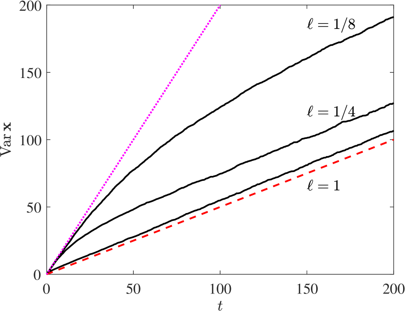
Figure 2: The mean-squared displacement (variance) $\operatorname{Var}\bm{x}$, averaged over $5\,000$ oblate non-swimming ($\bm{U}=\Omega=0$) active particles for various values of $\ell$. The upper dotted line is $4\times\tfrac{1}{2}(D_{\parallel}+D_{\perp})t$, and the bottom dashed line is $4D_{\mathrm{eff}}t$. As $\ell$ becomes smaller, there is a longer transient before the behavior begins to follow Eq. 21. This transient diverges as $\ell\rightarrow 0$. Parameter values: $m=I=.05$, $\sigma_{\parallel}=2$, $E_{\perp}=\sigma_{\perp}=\sigma_{\mathrm{r}}=1$, $E_{\parallel}=0$.

It is important to note that the ratio $\widetilde{D}_{0}/D_{\perp}$ is rarely negligible: all the dimensionless ratios appearing on the right of Eq. 23 are typically of order one. The transient time scale $D_{\mathrm{r}}^{-1}$ can be estimated by $a^{2}/D_{\perp}$, where $a$ is the particle size; if $D_{\mathrm{r}}^{-1}$ is very long, then $D_{\perp}$ was likely negligible to begin with. The modifications discussed in this paper are thus likely to be relevant in many applications.

So why haven’t these types of corrections been observed? Many authors simulate the ABP model directly, since the inertial equations (2) are expensive to solve due the small step size required, in which case the new effects are ruled out. Particle anisotropy is also seldom considered. Experimentally, diffusivities are measured directly from the distributions of displacements, and so any connection between the rotational and translational diffusivities is typically lost. One approach might be to obtain the covariance matrix $\widehat{\mathbb{A}}$ directly, by measuring the correlations between translational and rotational velocities. A nonzero correlation would indicate a coupling as predicted here.

In future work we will generalize the derivation to arbitrary three-dimensional active particles[25, 59], with the fluctuating force not necessarily applied on an axis of symmetry. There are several other possible extensions, such as the inclusion of multiple forces and torques acting on the body. The consequences to swim pressure [60, 61], run-and-tumble dynamics [1, 4], non-Newtonian swimming [62], velocity-dependent friction [63], and particle interactions [53, 64] also remain to be investigated.