EBMs Trained with Maximum Likelihood are Generator Models Trained with a Self-adverserial Loss

Abstract

Maximum likelihood estimation is widely used in training Energy-based models (EBMs). Training requires samples from an unnormalized distribution, which is usually intractable, and in practice, these are obtained by MCMC algorithms such as Langevin dynamics. However, since MCMC in high-dimensional space converges extremely slowly, the current understanding of maximum likelihood training, which assumes approximate samples from the model can be drawn, is problematic (Nijkamp et al., 2019). In this paper, we try to understand this training procedure by replacing Langevin dynamics with deterministic solutions of the associated gradient descent ODE. Doing so allows us to study the density induced by the dynamics (if the dynamics are invertible), and connect with GANs by treating the dynamics as generator models, the initial values as latent variables and the loss as optimizing a critic defined by the very same energy that determines the generator through its gradient. Hence the term - self-adversarial loss. We show that reintroducing the noise in the dynamics does not lead to a qualitative change in the behavior, and merely reduces the quality of the generator. We thus show that EBM training is effectively a self-adversarial procedure rather than maximum likelihood estimation.

1 Introduction

Energy-based models (EBMs) are likelihood-based generative models that model the unnormalized data density by assigning low energy to high-probability regions in the data space. Recently, by using neural network as the energy functions, deep EBMs (Xie et al., 2016; Du & Mordatch, 2019) are able to model complex data such as natural images (Xiao et al., 2021; Gao et al., 2021), 3D shapes (Xie et al., 2020) and texts (Deng et al., 2020). There are a variety of ways to train EBMs, including minimizing the KL-divergence (Du & Mordatch, 2019) or general F-divergence (Yu et al., 2020), score matching (Li et al., 2019) and contrastive estimation (Gutmann & Hyvärinen, 2010; Gao et al., 2020). Among them, the KL divergence minimization (equivalent to maximum likelihood estimation) is most widely used.

1.1 Maximum likelihood training of EBMs

To train an EBM of the form $p_{\theta}({\mathbf{x}})=\exp\left(-E_{\theta}({\mathbf{x}})\right)/Z_{\theta}$, where $E_{\theta}({\mathbf{x}})$ is the energy function with parameters $\theta$ and $Z_{\theta}=\int_{{\mathbf{x}}}\exp\left(-E_{\theta}({\mathbf{x}})\right)d{\mathbf{x}}$ is the normalizing constant, we can take the derivative of the negative log likelihood function $L(\theta)=\mathbb{E}_{{\mathbf{x}}\sim p_{d}({\mathbf{x}})}\left[-\log p_{\theta}({\mathbf{x}})\right]$ w.r.t to the model parameter $\theta$ (Woodford, 2006):

$$\partial_{\theta}L(\theta)=\mathbb{E}_{{\mathbf{x}}\sim p_{d}\left({\mathbf{x}}\right)}\left[\partial_{\theta}E_{\theta}\left({\mathbf{x}}\right)\right]-\mathbb{E}_{{\mathbf{x}}\sim p_{\theta}\left({\mathbf{x}}\right)}\left[\partial_{\theta}E_{\theta}\left({\mathbf{x}}\right)\right]$$ (1)

and minimize $L(\theta)$ by gradient descent. The second expectation in (1) can be empirically estimated by samples drawn from the model $p_{\theta}({\mathbf{x}})$ itself. However, sampling from $p_{\theta}({\mathbf{x}})$ is intractable and samples are usually drawn using MCMC. A commonly used MCMC algorithm is the Langevin dynamics (LD) (Neal, 1993). Given an initial sample ${\mathbf{x}}_{0}$, Langevin dynamics solves the SDE

$$d{\mathbf{x}}_{t}=-\frac{1}{2}\nabla_{{\mathbf{x}}}E_{\theta}({\mathbf{x}}_{t})dt+d\mathbf{w}_{t},$$ (2)

where $\mathbf{w}_{t}$ is Brownian motion. The discretized version, using the simplest Euler approximation yields:

$${\mathbf{x}}_{t+1}={\mathbf{x}}_{t}-\frac{\eta}{2}\nabla_{{\mathbf{x}}}E_{\theta}({\mathbf{x}}_{t})+\sqrt{\eta}\mathbf{\omega}_{t},$$ (3)

where $\mathbf{\omega}_{t}\sim\mathcal{N}(0,\mathbf{I})$ and $\eta$ is the step-size. Theoretically, we need to run the discretized LD with infinitely many steps and diminishing step sizes to obtain true samples. However, in practice, we usually run LD for finite number of steps with a fixed step size. After training, samples are obtained by running the same Langevin dynamics, typically with the same number of steps.

1.2 Alternative understanding of maximum likelihood training

Although the maximum likelihood training scheme is simple and intuitively appealing, we might still have not fully understood its mechanism. Since the convergence of MCMC is extremely difficult when the energy function is complicated, we cannot easily overlook the gap between running the LD in practice (usually called short-run LD) and truly obtaining samples from $p_{\theta}({\mathbf{x}})$. Indeed, some interesting observations are made from training the EBMs through maximum likelihood. Firstly, in practice the noise scale of LD is usually much smaller than the correct one in (3), which makes the LD similar to gradient descent (Du & Mordatch, 2019). Secondly, unless the shape of the energy function is carefully modified by introducing a base distribution as done in Nijkamp et al. (2020a); Xiao et al. (2020), LD usually does not mix, i.e., samples obtained by running longer LD get trapped in different local modes instead of traversing between modes. Probably as a consequence, the initial points ${\mathbf{x}}_{0}$ contain information about the final outcome, and therefore short-run LD is observed to be capable of reconstructing the data and interpolating different samples (Nijkamp et al., 2019). In addition, sometimes while we can obtain good samples by running short-run LD, the density of the EBMs can be drastically different from the true data densities (e.g., Figure 2 of Gao et al. (2021)). These observations suggest that running short-run LD may be fundamentally different from obtaining samples from the EBMs, and therefore the maximum likelihood explanation for the training procedure may be invalid.

Nijkamp et al. (2019) first study the intriguing properties of short-run LD. They conjecture that the short-run LD behaves more like a generator model, and try to explain the maximum likelihood training by introducing $q_{\theta}$, the marginal distribution of the sample after running $K$ steps of LD starting from a fixed initial distribution. However, they do not study $q_{\theta}$ with an explicit formulation. In this paper, we follow their work to provide an alternative understanding of the maximum likelihood training of EBMs. In particular, we replace the LD sampling with noise-free dynamics, so that the output samples are produced by a deterministic transformation of the initial points. In this case, we regard the dynamic as a generator model, and the initial points as latent variables. By ensuring that the generator is invertible, we can explicitly study the density of the distribution induced by the sampling dynamics (where the randomness is entirely determined by the initial points). In addition, by treating the sampling dynamics as a generator model, we find that we can improve the sample quality by adding the generator loss term from GANs to the original loss.

2 Noise-free sampling dynamics as flow model

In this section, we demonstrate how to explicitly obtain the density induced by the noise-free sampling dynamics by enforcing invertibility. We start by replacing the Langevin dynamics in (2) with the noise-free gradient descent ODE:

$${\mathbf{x}}^{\prime}(t)=-\nabla_{\mathbf{x}}E_{\theta}({\mathbf{x}}(t)),\quad{\mathbf{x}}(0)={\mathbf{x}}_{0},\quad t\in[0,T],$$ (4)

which is guaranteed to produce an invertible map under very mild conditions on $E$, and we can write the continuous flow (Chen et al., 2018; Grathwohl et al., 2018):

$${\mathbf{x}}_{T}=G^{T}_{\theta}({\mathbf{x}}_{0})=\operatorname{ODESolve}(-\nabla_{\mathbf{x}}E_{\theta}({\mathbf{x}}(t)),{\mathbf{x}}_{0},[0,T]).$$ (5)

Since there is no noise term, given ${\mathbf{x}}_{0}$, the process can be represented by a deterministic generator model with latent variable ${\mathbf{x}}_{0}$. We want to emphasize that $T$ is an important component of the generator model, and we should use roughly the same T when sampling. Moreover, as $G^{T}_{\theta}({\mathbf{x}}_{0})$ is invertible, the likelihood along the path can be obtained by instantaneous change of variables formula (Chen et al., 2018), and the log likelihood of data ${\mathbf{x}}$ under the flow model can be computed by

$$\log p({\mathbf{x}})=\log p({\mathbf{x}}_{0})+\int_{0}^{T}\text{tr}\left[\nabla_{{\mathbf{x}}{\mathbf{x}}}E_{\theta}({\mathbf{x}}(t))\right]dt.$$ (6)

As a special case, the forward Euler solver for this equation yields:

$${\mathbf{x}}_{t+1}={\mathbf{x}}_{t}-\frac{\eta}{2}\nabla_{{\mathbf{x}}}E_{\theta}({\mathbf{x}}_{t}),\quad t=0,1,\cdots,K-1,$$ (7)

with initialization ${\mathbf{x}}_{0}$ from some fixed simple distribution $p_{0}$ in $\mathbb{R}^{d}$ such as the standard Gaussian. In particular, $G_{\theta}({\mathbf{x}}_{0}):\mathbb{R}^{d}\rightarrow\mathbb{R}^{d}$ is a residual flow (Behrmann et al., 2019):

$${\mathbf{x}}_{K}=G_{\theta}({\mathbf{x}}_{0})=(I-\frac{\eta}{2}\nabla_{{\mathbf{x}}}E_{\theta})^{K}({\mathbf{x}}_{0}).$$ (8)

$G_{\theta}({\mathbf{x}}_{0})$ is guaranteed to be invertible if $\operatorname{lip}\left(\frac{\eta}{2}\nabla_{{\mathbf{x}}}E_{\theta})\right)<1$ (Behrmann et al., 2019). This holds as long as $\nabla_{{\mathbf{x}}}E_{\theta}$ has bounded Lipschitz constant and the step size $\eta$ is sufficiently small. However, it is still difficult to choose the step size that ensures invertibility, and therefore, we generalize $G_{\theta}({\mathbf{x}}_{0})$ to be any numerical solution to the initial value ODE problem (4).

To summarize, we train the energy network $E_{\theta}$ by doing the gradient update (1) with negative samples obtained from (5). After training, we can obtain new samples by running (5), and compute the likelihood of data point ${\mathbf{x}}$ by solving the ODE (4) in the reverse direction to find the corresponding initial point ${\mathbf{x}}_{0}$ and then apply (6).

3 Connection with W-GAN and the generator loss term

It is well known that the maximum likelihood training of EBMs is closely related to the training of Wasserstein-GANs (Arjovsky et al., 2017), where the objective for the discriminator $D$ (assuming $D$ is $1$-Lipschitz) is

$$\max_{D}\underset{{\mathbf{x}}\sim p_{D}}{\mathbb{E}}\left[D({\mathbf{x}})\right]-\underset{\tilde{{\mathbf{x}}}\sim p_{G}}{\mathbb{E}}\left[D(\tilde{{\mathbf{x}}})\right].$$ (9)

The gradient of (9) is (up to a sign) very similar to (1) except that here the negative samples are drawn from the generator, while in (1), the negative samples are drawn from the EBM itself. Note that the sign does not matter as we can model the negative energy instead. W-GANs use the discriminator $D$ to contrast true data and samples generated by the generator $G$, while EBMs use the energy function $E$ to contrast true data and samples generated by $E$ itself implicitly through MCMC. Therefore, the maximum likelihood training of EBMs can be described as a self-adversarial game.

In W-GAN, after the discriminator is updated by (9), the generator $G$ is then updated by

$$\max_{G}\underset{\tilde{{\mathbf{x}}}\sim p_{G}}{\mathbb{E}}\left[D(\tilde{{\mathbf{x}}})\right].$$ (10)

In other words, it maximizes the discriminator’s output for fake samples generated by $G$. Strictly speaking, there is no corresponding loss term in the training of EBMs, as the sampling is done by MCMC rather than deterministic mapping. However, as discussed in section 2, in practice the sampling process can be seen as a generator model with initial points as latent variables. In this case, we actually have an explicit generator $G_{\theta}$ defined in (5), and therefore we can update the parameter of $G_{\theta}$ (which is just $\theta$) by the following objective:

$$\min_{\theta}E_{\text{sg}(\theta)}(G_{\theta}({\mathbf{x}}_{0})),$$ (11)

where ${\mathbf{x}}_{0}$ is the latent variables sampled from $p_{0}$, and sg($\cdot$) is the stop gradient operation. Here we stop the gradient of $E_{\theta}$ because we only want to differentiate through the generation process.

Hence, we propose to add the extra update step for $G_{\theta}$ at each iteration, so that we are essentially training a W-GAN whose discriminator and generator share the same set of parameters, and conjecture that the adversarial training will improve the sample quality.

One modification is made for the implementation. Typically when training GANs, we alternate the update of the parameters of the discriminator and the generator and hence two batches of samples are generated. This can be slow in our case as drawing samples requires iterative updates. Therefore, we use the same batch of samples to update $E_{\theta}$ and $G_{\theta}$, and since we only have one set of parameters $\theta$, it is equivalent to optimizing the following objective:

$$\min_{\theta}E_{\theta}({\mathbf{x}})-E_{\theta}(G_{\text{sg}(\theta)}({\mathbf{x}}_{0}))+E_{\text{sg}(\theta)}(G_{\theta}({\mathbf{x}}_{0})),\quad{\mathbf{x}}\sim p_{D},{\mathbf{x}}_{0}\sim p_{0}.$$ (12)

We will empirically study the effectiveness of this training objective in section 5.2.

4 Related Work

Our work is closely related to earlier studies on the properties of ML training EBMs with short-run non-convergent MCMC (Nijkamp et al., 2019; 2020b), where they illustrate through experiments that the short-run LD behaves more like a generator model, and in particular Nijkamp et al. (2019) provide a moment matching framework for explaining the mechanism behind the maximum likelihood training. In addition, Xie et al. (2018; 2020) propose MCMC teaching, where a separate generator is trained to absorb the process of LD sampling. This suggests that their method is based on the assumption that LD used in practice can be represented as a generator model. Additionally, Han et al. (2019) provides a probabilistic way to deal with EBM without MCMC. We take a further step from them to explicitly study the properties of the generator models.

Since our noise-free sampling dynamics can yield an invertible gradient flow , our work is related to the concept of generative gradient flows (Zhang et al., 2018; Huang et al., 2021). In addition, Song et al. (2021) show that the stochastic dynamics of score based generative models (Song & Ermon, 2019; Ho et al., 2020) are equivalent to specific deterministic ODE flows Chen et al. (2018); Grathwohl et al. (2018). However, such equivalence cannot be easily established for Langevin diffusion. Pang et al. (2020) connects EBM and generator model, but what they do is learning an EBM prior for the generator. Finally, our work is related to previous work that connects GANs with EBMs (Che et al., 2020; Song et al., 2020; Ansari et al., 2021) or invertible flows (Grover et al., 2018). In particular, Grover et al. (2018) use invertible structure, such as real-NVP (Dinh et al., 2016), for the generator of GANs, but they focus on hybrid training with adversarial and maximum likelihood objectives.

5 Results

In this section, we conduct experiments to verify our proposed methods and arguments in section 2 and 3. Specifically, we train energy functions on 2d-toy data and image data by replacing the MCMC sampling with deterministic dynamics. Throughout the experiments, we initialize the dynamics with noise sampled from standard Gaussian distribution. We do not use persistent sampling, as we want to interpret the model as a generator with fixed prior. The deterministic dynamics can be simply defined by (7), or more generally the path to solve the ODE as in (5). In particular, we need to use the latter method if we want to compute the density induced by the dynamics. More experimental detail can be found in appendix A.

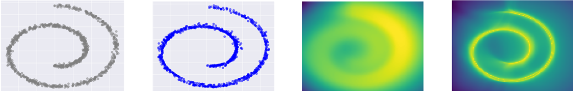
(a) Swiss roll

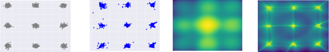
(b) Gaussian grid

Figure 1: For each toy dataset, column 1: samples from the true data distribution; column 2: samples from the ODE flow; column 3: (unnormalized) log density of the EBM by plotting the value of $-E_{\theta}({\mathbf{x}})$; column 4: log density of the ODE flow computed by (6). The spurious connections between components will visually disappear if we take exponential (see Appendix B). We plot log density because the sampling dynamics directly use it.

5.1 2D toy data

We use the Swiss roll and 9 Gaussian mixture grid as the true distributions, and our energy function $E_{\theta}:\mathbb{R}^{2}\rightarrow\mathbb{R}$ is a simple neural network with several fully connected layers. We use the neural ODE formulation and solve the ODE in (4) with the default Dormand–Prince solver as in Chen et al. (2018). In Figure 1, we plot the samples obtained from solving the ODE (5). We also plot the log density of the ODE flow and the value of the negative energy function (which is the unnormalized log density of the corresponding EBM) in the same figure. We observe that we can obtain good samples, even though the densities of the EBMs are not close to the ground truth densities. In contrast, the density functions induced by the ODE flow captures the densities the true data distributions very well. We also train EBMs with valid MCMC sampling with noise term, and plot the density functions and generated samples in appendix B. There we make a similar observation that the densities of EBMs do not match the data distribution.

These observations provide evidence that maximum likelihood training of EBMs is actually training a gradient flow model. Since the density defined by the final energy function completely fails to capture the true data density, arguments that running the sampling dynamics draws samples from the EBM is certainly incorrect; instead, we show that the dynamic itself is the generative model to sample from, as its density matches the shape of the true density.

In addition, we also train the ODE flows with the same formulation and structure using the maximum likelihood objective (where the likelihood is defined in (6)) and compare the obtained data likelihood with that of the flows trained by the EBM objective. For the ODE flows trained by maximum likelihood, the test data log likelihood (averaged over 10000 test samples) is -0.69 nats on Swiss roll and -1.47 nats on Gaussian grid. The test data likelihood of the ODE flows trained by the EBM objective is -0.86 nats and -1.95 nats on these two datasets, respectively. As expected, the flows directly trained by maximizing data likelihood have higher test likelihood, but the flows trained by the EBM objective still perform reasonably well.

5.2 Image data

Experiments on toy data reveal that the maximum likelihood training of EBMs may actually lead to training generator or flow models. If this is true, then the noise term used in Langevin dynamics may be unnecessary or even harmful. We confirm this by studying the sample quality on common image datasets including MNIST, Fashion-MNIST, CIFAR-10 and CelebA. For simplicity, our energy functions are simple convolutional nets instead of more complex residual networks used in Du & Mordatch (2019); Xiao et al. (2021), and therefore we only compare relative performances.

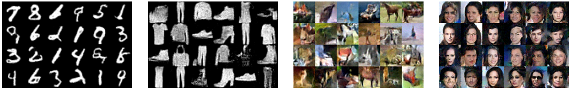
(a) EBMs w/ noisy dynamics

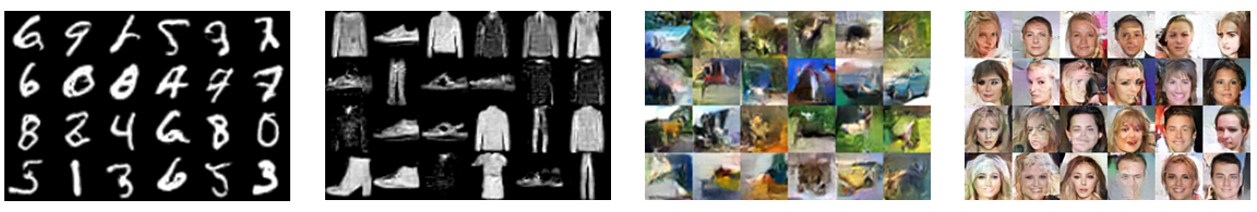
(b) EBMs w/ noise-free dynamics

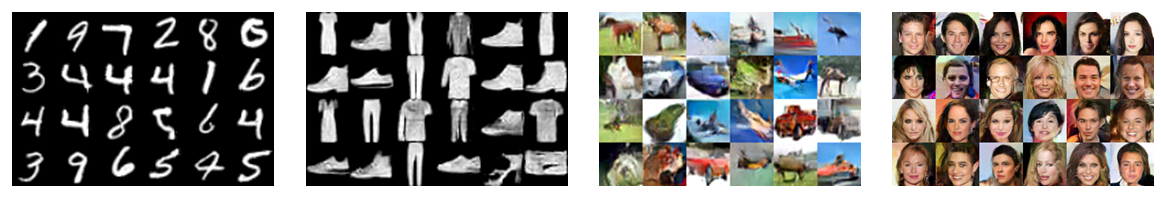
(c) EBMs w/ noise-free dynamics + generator loss

Figure 2: Qualitative samples of models with noisy or noise-free sampling dynamics, and models with extra loss to update the generator defined by the dynamics.

We train energy functions using the gradient update in (1), where the samples are generated by either noisy or noise-free sampling dynamics. For noise-free dynamics, we use the gradient descent formulation in (7) instead of the neural ODE formulation, because we only want to study the effect of noise while keeping all other factors the same. For noisy sampling dynamics, we reduce the noise scale as done in almost all other work, otherwise the training diverges quickly. We report the FID scores (Heusel et al., 2017) in Table LABEL:fid_table, and qualitative samples in Figure 2 and appendix D. We observe that EBMs trained with noise-free dynamics indeed obtain better sample quality on all datasets. Besides, we plot the loss curves in Appendix C, and we find that removing the noise significantly improves the training stability. Even with reduced noise scale, training EBMs with noisy sampling dynamics may still diverges during training. These results suggest that the noise term in sampling dynamics may have negative effects, which further supports the argument that the we should treat the model as a generator defined by the gradient of the energy instead of an EBM.

Table 1: FID scores on image datasets for different models

	MNIST	Fashion-MNIST	CIFAR-10	CelebA
EBM w/ noisy dynamic	15.4	61.7	70.4	69.6
EBM w/ noise-free dynamic	11.7	50.1	61.6	56.6
+ Generator loss	7.7	40.6	47.9	34.8

Treating the noise-free dynamics as generator models, we further apply the additional adversarial loss term for the W-GAN generator update discussed in section 3. In particular, we train the model with loss in (12). We report the FID in the last line of Table LABEL:fid_table, where we find the generator update significantly improves the sample quality. Qualitative samples are shown in Figure 2 and additional samples in appendix D. This experiment shows that the noise-free dynamics is indeed a generator, and we can use it to train GANs.

6 Conclusion and Discussion

In this paper, we provide new insights to understand the maximum likelihood training of EBMs. We believe that instead of training EBMs, the maximum likelihood objective actually trains generator models through a self-adversarial mechanism. The generator model is defined implicitly by the gradient of the energy network, and we study the property of the generator model by removing the noise in the MCMC sampling dynamics. We conduct experiments to justify our thoughts and make the following observations:

• On toy data, the density function induced by the invertible noise-free dynamics is close to the shape of the true data density, while the density of the EBM with corresponding energy function fails to capture the true density.

• On image datasets, we observe that removing the noise in the LD improves sample quality and training stability.

• The sample quality can be further improved by introducing the generator update discussed in section 3, i.e., making the self-adversarial game into an adversarial game.

These observations together suggest that the mechanism behind the ML training of EBMs is to train a generator or gradient flow model, and we can benefit from removing the noise in the sampling dynamics. As a result, given the difficulty of running MCMC in high dimensions, we should study the convergence of MCMC sampling in high dimensions more carefully, and probably focus more on training techniques without sampling, if our goal is to train valid energy-based models.

Appendix A Experimental settings

In this section, we introduce detailed settings of our experiments.

A.1 2D toy data

On 2D toy data, we use a 5-layer fully connected networks with 256 hidden units and swish activation function. We train our models with Adam optimizer, with constant learning rate $1e-3$. The models are trained for 3000 iterations with batch size 800.

We draw negative samples by solving the ODE in (5). To do so, we use the solver implemented by Chen et al. (2018). We set the initial value to random samples from 2-d standard Gaussian distribution. We use the default dopri5 solver, $T\in[0,0.2]$, and numerical error tolerance tolerance $1e-5$. After training, samples are drawn by solving the same neural ODE.

A.2 Image data

We resize MNIST and Fashion-MNIST to $32\times 32$. The network structures are presented in Table 2. We train all models with Adam optimizer with learning rate $5e-4$ and batch size $64$. As we mention in the main text, the training of EBMs with noisy dynamics is unstable and it will diverge after certain number of iterations. This is also observed in Du & Mordatch (2019) and Xiao et al. (2021). Therefore, we follow their setting to train the EBMs until divergence. For EBMs trained with noise-free dynamics, we found the training to be more stable. We set the number of training iterations similar to that of EBMs with noisy dynamics. In particular, we train 8000 iterations for MNIST and Fashion-MNIST, 40000 iterations for CIFAR-10 and 30000 iterations for CelebA. To draw negative samples, we set the step size to be $0.1$ and number of steps to be $40$ for MNIST/Fashion-MNIST and $60$ for CIFAR-10 and CelebA. For the noisy sampling dynamics, we set the noise scale to be $0.1$.

For the extra GAN loss, we need to store the gradient while running the gradient descent steps (7). This can be done by setting the create graph option when computing the gradient in PyTorch’s auto differential package (Paszke et al., 2019).

MNIST	CIFAR-10	CelebA
$3\times 3$ $\text{Conv}_{\text{nf}}$ Stride $1$	$3\times 3$ $\text{Conv}_{\text{nf}}$ Stride $1$	$3\times 3$ $\text{Conv}_{\text{nf}}$ Stride $1$
$4\times 4$ $\text{Conv}_{2\times\text{nf}}$ Stride $2$	$4\times 4$ $\text{Conv}_{2\times\text{nf}}$ Stride $2$	$4\times 4$ $\text{Conv}_{2\times\text{nf}}$ Stride $2$
$4\times 4$ $\text{Conv}_{2\times\text{nf}}$ Stride $2$	$4\times 4$ $\text{Conv}_{4\times\text{nf}}$ Stride $2$	$4\times 4$ $\text{Conv}_{4\times\text{nf}}$ Stride $2$
$4\times 4$ $\text{Conv}_{2\times\text{nf}}$ Stride $2$	$4\times 4$ $\text{Conv}_{8\times\text{nf}}$ Stride $2$	$4\times 4$ $\text{Conv}_{8\times\text{nf}}$ Stride $2$
Faltten, FC layer to scalar	Faltten, FC layer to scalar	$4\times 4$ $\text{Conv}_{16\times\text{nf}}$ Stride $2$
		Faltten, FC layer to scalar

Table 2: Network structures for different datasets. nf means number of filters. For MNIST, Fashion MNIST and CelebA, nf = 32; for CIFAR-10, nf = 64. Swish activation is applied after each convolutional layer.

Appendix B Additional results on 2D toy data

In Figure 3, we plot the samples and (unnormalized) density of EBMs trained with noisy sampling dynamics (finite steps of Langevin dynamics). The shown samples are generated by running the same Langevin dynamics. Note that we cannot plot the density induced by the dynamic itself as the noise term makes it not invertible. However, we have similar observations as in Figure 1. While the sample quality is good, the density of EBMs completely fail to match the true data distribution. We notice that Gao et al. (2021) make similar observations (see their Figure 2).

This suggest that even in the usual case where EBMs are trained and sampled with LD, samples are actually generated from a (noise injected) generator model instead of the EBM. Therefore, the mechanism behind maximum likelihood training of EBMs is actually training generator models implicitly defined by the sampling dynamics.

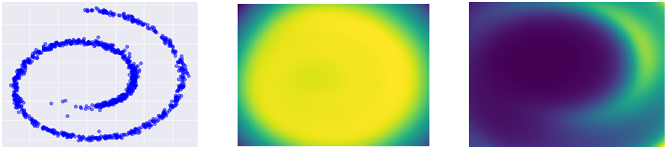
(a) Swiss roll

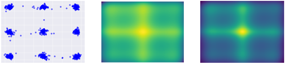
(b) Gaussian grid

Figure 3: Results of EBMs trained and sampled from using noisy dynamics on toy data. For each sub-figure, we plot the left: samples obtained from running Langevin dynamics, middle: (unnormalized) log density of the EBM , and right: normalized density of the EBM, where the normalization constant is estimated by numerical integration.

We also plot the normalized density of the EBMs and gradient flows in Figure 4, where we observe that the spurious high density region shown in the log density plot in Figure 1 disappears, and we still find that the density of the gradient flows captures the true density much better than that of the EBMs.

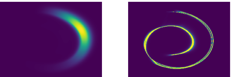
(a) Swiss roll

(b) Gaussian grid

Figure 4: For each sub-figure, left: normalized density of the EBM, and right: density of the gradient flow.

Appendix C Loss curves

(a) EBMs w/ noisy dynamics

(b) EBMs w/ noisy dynamics, first 20000 iterations

(c) EBMs w/ noise-free dynamics

(d) EBMs w/ noise-free dynamics + generator loss

Figure 5: Plots of loss curves on CIFAR-10 dataset. (a): When sampling using the noisy MCMC, the training diverges after 20000 iterations. (b): For better visualization, we plot the loss curve for the first 20000 iterations. (c): When using noise-free dynamics, the training is more stable. (d): With the additional generator loss, although we see some jumps on the loss curve, the training is overall stable.

In Figure 5, we plot the loss curve along the training of models with noisy or noise-free dynamics on CIFAR-10. We observe that for both models, the losses oscillate around zero, as observed in Nijkamp et al. (2020b). However, the model trained with noisy dynamics diverges after 20000 iterations, while the the training of model with noise-free dynamics is much more stable. In addition, we observe that adding the extra generator loss as discussed in section 3 does not affect the training stability.

Appendix D Additional results on image data

In Figure 6, 7 and 8, we present additional qualitative samples corresponding to Figure 2 in the main text.

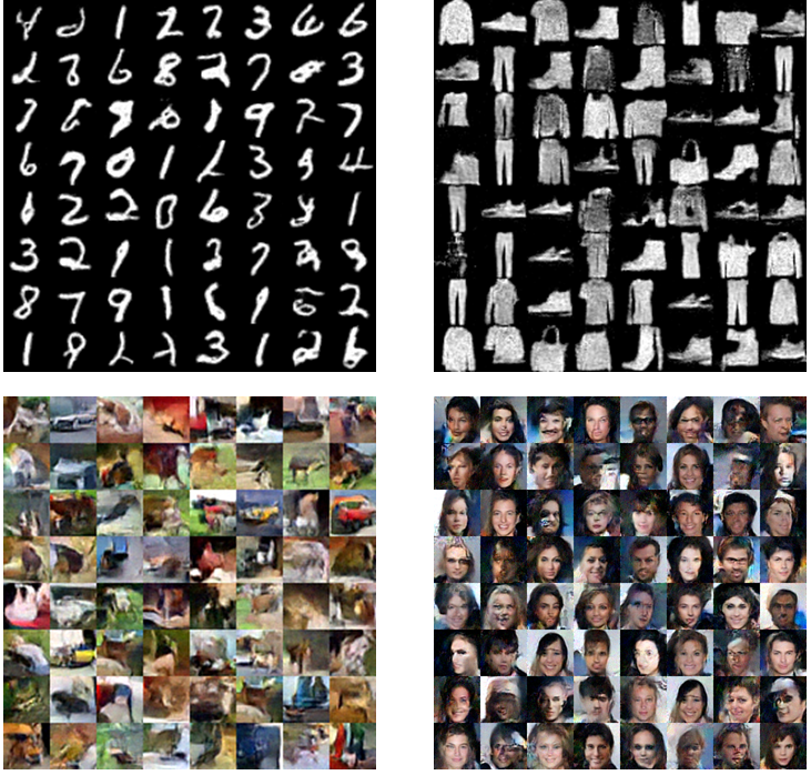
Figure 6: Additional samples from EBMs w/ noisy dynamics

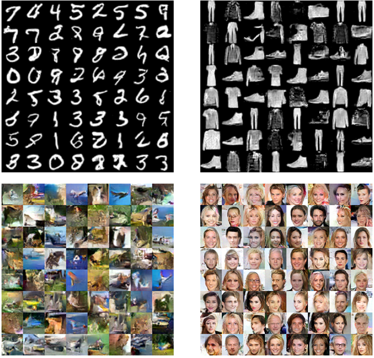
Figure 7: Additional samples from EBMs w/ noise-free dynamics

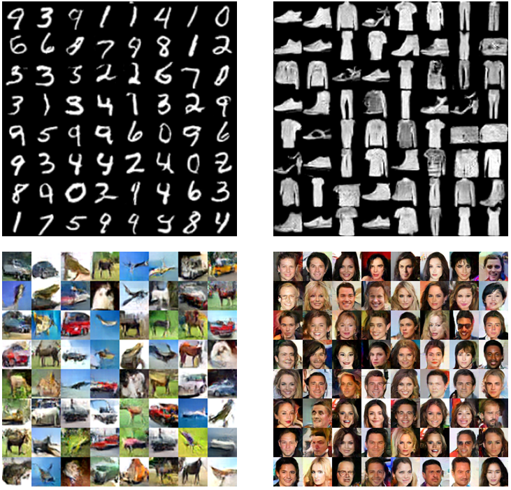
Figure 8: Additional samples from EBMs w/ noise-free dynamics plus extra generator loss

References

- Ansari et al. (2021) Abdul Fatir Ansari, Ming Liang Ang, and Harold Soh. Refining deep generative models via discriminator gradient flow. In International Conference on Learning Representations, 2021. URL https://openreview.net/forum?id=Zbc-ue9p_rE.
- Arjovsky et al. (2017) Martin Arjovsky, Soumith Chintala, and Léon Bottou. Wasserstein generative adversarial networks. In International conference on machine learning, pp. 214–223. PMLR, 2017.
- Behrmann et al. (2019) Jens Behrmann, Will Grathwohl, Ricky T. Q. Chen, David Duvenaud, and Joern-Henrik Jacobsen. Invertible residual networks. In Kamalika Chaudhuri and Ruslan Salakhutdinov (eds.), Proceedings of the 36th International Conference on Machine Learning, volume 97 of Proceedings of Machine Learning Research, pp. 573–582. PMLR, 09–15 Jun 2019. URL http://proceedings.mlr.press/v97/behrmann19a.html.
- Che et al. (2020) Tong Che, Ruixiang Zhang, Jascha Sohl-Dickstein, Hugo Larochelle, Liam Paull, Yuan Cao, and Yoshua Bengio. Your gan is secretly an energy-based model and you should use discriminator driven latent sampling. arXiv preprint arXiv:2003.06060, 2020.
- Chen et al. (2018) Ricky TQ Chen, Yulia Rubanova, Jesse Bettencourt, and David Duvenaud. Neural ordinary differential equations. arXiv preprint arXiv:1806.07366, 2018.
- Deng et al. (2020) Yuntian Deng, Anton Bakhtin, Myle Ott, Arthur Szlam, and Marc’Aurelio Ranzato. Residual energy-based models for text generation. arXiv preprint arXiv:2004.11714, 2020.
- Dinh et al. (2016) Laurent Dinh, Jascha Sohl-Dickstein, and Samy Bengio. Density estimation using real nvp. arXiv preprint arXiv:1605.08803, 2016.
- Du & Mordatch (2019) Yilun Du and Igor Mordatch. Implicit generation and modeling with energy based models. In Advances in Neural Information Processing Systems, pp. 3608–3618, 2019.
- Gao et al. (2020) Ruiqi Gao, Erik Nijkamp, Diederik P Kingma, Zhen Xu, Andrew M Dai, and Ying Nian Wu. Flow contrastive estimation of energy-based models. In Proceedings of the IEEE/CVF Conference on Computer Vision and Pattern Recognition, pp. 7518–7528, 2020.
- Gao et al. (2021) Ruiqi Gao, Yang Song, Ben Poole, Ying Nian Wu, and Diederik P Kingma. Learning energy-based models by diffusion recovery likelihood. In International Conference on Learning Representations, 2021. URL https://openreview.net/forum?id=v_1Soh8QUNc.
- Grathwohl et al. (2018) Will Grathwohl, Ricky TQ Chen, Jesse Bettencourt, Ilya Sutskever, and David Duvenaud. Ffjord: Free-form continuous dynamics for scalable reversible generative models. arXiv preprint arXiv:1810.01367, 2018.
- Grover et al. (2018) Aditya Grover, Manik Dhar, and Stefano Ermon. Flow-gan: Combining maximum likelihood and adversarial learning in generative models. In Proceedings of the AAAI Conference on Artificial Intelligence, volume 32, 2018.
- Gutmann & Hyvärinen (2010) Michael Gutmann and Aapo Hyvärinen. Noise-contrastive estimation: A new estimation principle for unnormalized statistical models. In Proceedings of the Thirteenth International Conference on Artificial Intelligence and Statistics, pp. 297–304, 2010.
- Han et al. (2019) Tian Han, Erik Nijkamp, Xiaolin Fang, Mitch Hill, Song-Chun Zhu, and Ying Nian Wu. Divergence triangle for joint training of generator model, energy-based model, and inferential model. In Proceedings of the IEEE/CVF Conference on Computer Vision and Pattern Recognition, pp. 8670–8679, 2019.
- Heusel et al. (2017) Martin Heusel, Hubert Ramsauer, Thomas Unterthiner, Bernhard Nessler, Günter Klambauer, and Sepp Hochreiter. Gans trained by a two time-scale update rule converge to a nash equilibrium. 2017.
- Ho et al. (2020) Jonathan Ho, Ajay Jain, and Pieter Abbeel. Denoising diffusion probabilistic models. arXiv preprint arXiv:2006.11239, 2020.
- Huang et al. (2021) Chin-Wei Huang, Ricky T. Q. Chen, Christos Tsirigotis, and Aaron Courville. Convex potential flows: Universal probability distributions with optimal transport and convex optimization. In International Conference on Learning Representations, 2021. URL https://openreview.net/forum?id=te7PVH1sPxJ.
- Li et al. (2019) Zengyi Li, Yubei Chen, and Friedrich T Sommer. Learning energy-based models in high-dimensional spaces with multi-scale denoising score matching. arXiv preprint arXiv:1910.07762, 2019.
- Neal (1993) Radford M Neal. Probabilistic inference using Markov chain Monte Carlo methods. 1993.
- Nijkamp et al. (2019) Erik Nijkamp, Mitch Hill, Song-Chun Zhu, and Ying Nian Wu. Learning non-convergent non-persistent short-run mcmc toward energy-based model. arXiv preprint arXiv:1904.09770, 2019.
- Nijkamp et al. (2020a) Erik Nijkamp, Ruiqi Gao, Pavel Sountsov, Srinivas Vasudevan, Bo Pang, Song-Chun Zhu, and Ying Nian Wu. Learning energy-based model with flow-based backbone by neural transport mcmc. arXiv preprint arXiv:2006.06897, 2020a.
- Nijkamp et al. (2020b) Erik Nijkamp, Mitch Hill, Tian Han, Song-Chun Zhu, and Ying Nian Wu. On the anatomy of mcmc-based maximum likelihood learning of energy-based models. In Proceedings of the AAAI Conference on Artificial Intelligence, volume 34, pp. 5272–5280, 2020b.
- Pang et al. (2020) Bo Pang, Tian Han, Erik Nijkamp, Song-Chun Zhu, and Ying Nian Wu. Learning latent space energy-based prior model. arXiv preprint arXiv:2006.08205, 2020.
- Paszke et al. (2019) Adam Paszke, Sam Gross, Francisco Massa, Adam Lerer, James Bradbury, Gregory Chanan, Trevor Killeen, Zeming Lin, Natalia Gimelshein, Luca Antiga, et al. Pytorch: An imperative style, high-performance deep learning library. arXiv preprint arXiv:1912.01703, 2019.
- Song & Ermon (2019) Yang Song and Stefano Ermon. Generative modeling by estimating gradients of the data distribution. arXiv preprint arXiv:1907.05600, 2019.
- Song et al. (2021) Yang Song, Jascha Sohl-Dickstein, Diederik P Kingma, Abhishek Kumar, Stefano Ermon, and Ben Poole. Score-based generative modeling through stochastic differential equations. In International Conference on Learning Representations, 2021. URL https://openreview.net/forum?id=PxTIG12RRHS.
- Song et al. (2020) Yuxuan Song, Qiwei Ye, Minkai Xu, and Tie-Yan Liu. Discriminator contrastive divergence: Semi-amortized generative modeling by exploring energy of the discriminator. arXiv preprint arXiv:2004.01704, 2020.
- Woodford (2006) Oliver Woodford. Notes on contrastive divergence. Department of Engineering Science, University of Oxford, Tech. Rep, 2006.
- Xiao et al. (2020) Zhisheng Xiao, Qing Yan, and Yali Amit. Exponential tilting of generative models: Improving sample quality by training and sampling from latent energy. arXiv preprint arXiv:2006.08100, 2020.
- Xiao et al. (2021) Zhisheng Xiao, Karsten Kreis, Jan Kautz, and Arash Vahdat. Vaebm: A symbiosis between variational autoencoders and energy-based models. In International Conference on Learning Representations, 2021. URL https://openreview.net/forum?id=5m3SEczOV8L.
- Xie et al. (2020) J. Xie, Z. Zheng, R. Gao, W. Wang, S. C. Zhu, and Y. N. Wu. Generative voxelnet: Learning energy-based models for 3d shape synthesis and analysis. IEEE Transactions on Pattern Analysis and Machine Intelligence, pp. 1–1, 2020. doi: 10.1109/TPAMI.2020.3045010.
- Xie et al. (2016) Jianwen Xie, Yang Lu, Song-Chun Zhu, and Yingnian Wu. A theory of generative convnet. In International Conference on Machine Learning, pp. 2635–2644, 2016.
- Xie et al. (2018) Jianwen Xie, Yang Lu, Ruiqi Gao, and Ying Nian Wu. Cooperative learning of energy-based model and latent variable model via mcmc teaching. In Proceedings of the AAAI Conference on Artificial Intelligence, volume 32, 2018.
- Xie et al. (2020) Jianwen Xie, Zilong Zheng, and Ping Li. Learning energy-based model with variational auto-encoder as amortized sampler. arXiv preprint arXiv:2012.14936, 2020.
- Yu et al. (2020) Lantao Yu, Yang Song, Jiaming Song, and Stefano Ermon. Training deep energy-based models with f-divergence minimization. In International Conference on Machine Learning, pp. 10957–10967. PMLR, 2020.
- Zhang et al. (2018) Linfeng Zhang, Lei Wang, et al. Monge-ampere flow for generative modeling. arXiv preprint arXiv:1809.10188, 2018.