New rotating AdS/dS black holes in $\mathrm{f(R)}$ gravity

Abstract

It is known that  general relativity (GR) theory is not consistent with the latest observations.  The modified gravity of GR known as $\mathrm{f(R)}$  where  $\mathrm{R}$ is the Ricci scalar, is considered  to be a  good candidate for dealing with the anomalies present in classical  GR. In this context, we study static rotating uncharged anti-de Sitter and de Sitter (AdS and dS) black holes (BHs) using  $\mathrm{f(R)}$  theory without assuming any constraints on the Ricci scalar or on  $\mathrm{f(R)}$. We derive  BH solutions depend on  the convolution function and deviate from the AdS/dS Schwarzschild  BH solution of GR. Although the field equations have no dependence on the cosmological constant, the BHs are characterized by an effective cosmological constant that  depends on the convolution function. The asymptotic form of this BH solution depends on the gravitational mass of the system and on extra terms that lead to BHs being different from GR BHs but to correspond to GR BHs under certain conditions. We also investigate how these extra terms are responsible for making the singularities of the invariants milder than those of  the GR BHs. We study some physical properties of the BHs from the point of view of thermodynamics and show that there is an outer event horizon in addition to the inner Cauchy horizons. Among other things  we show that our BH solutions satisfy the first law of thermodynamics. To check the stability of these BHs we use the geodesic deviations and  derive the stability conditions.  Finally,  using the odd-type mode it is shown that all the derived BHs are stable and have a radial speed equal to one.

I Introduction

Extended gravitational theories (EGTs) have become topic of interest Capozziello and Faraoni (2011); Capozziello and De Laurentis (2011); Nojiri and Odintsov (2011); Olmo (2011) since the discovery that the expansion of the universe is accelerating Riess et al. (1998). These EGTs are considered to be a tool that can deal with issues that GR cannot handle while at the same time preserving the success of GR at the solar system as well as the astrophysical scale Perlmutter et al. (1999); Riess et al. (1998, 2004); Hirata et al. (1987); Dodelson and Widrow (1994); Cole et al. (1994).  There are many ways to extend GR: one is to include a nonlinear function of the Ricci or torsion scalars in the Hilbert Einstein  action Schmidt (2006); Awad et al. (2018). The idea of a modified GR was proposed soon after Einstein proposed his GR. This was due to GR’s shortcoming  in terms of renormalization, which makes it incompatible with quantum mechanics Weyl (1919); Eddington (1988). Later  Utiyama and DeWitt showed that for GR theory to be compatible with  one–loop renormalization, its action must contain higher–order curvature terms Utiyama and DeWitt (1962); Utiyama (1956). Generally, any form of the function $\mathrm{f(R)}$ must be consistent with the results of GR at the solar–system scale and must also: (a) be free of ghosts (b) give the correct result at the Newtonian and post-Newtonian limit, (c) produce the correct cosmological dynamics, (d) fully resolve the Cauchy problem and (e) produce cosmological perturbations that are consistent with the cosmic microwave background radiation and large-scale cosmic structures Capozziello and Faraoni (2011).

$\mathrm{f(R)}$ theory is considered to be an important EGTs generic Einstein–Hilbert action by including the higher–order Ricci scalar as well as the Ricci and  Riemann tensors or their derivatives Buchdahl (1970); Starobinsky (1980).  $\mathrm{f(R)}$ has succeeded in explaining dark energy and dark matter. Much work has therefore been done in relation to $\mathrm{f(R)}$: this has included astrophysics and cosmological studies Shah and Samanta (2019); Nojiri et al. (2019); Odintsov and Oikonomou (2019a, b); Nascimento et al. (2019); Miranda et al. (2019); Astashenok et al. (2019); Elizalde et al. (2019a, b); Chen (2019); Sbisà et al. (2019); Bombacigno and Montani (2019); Capozziello et al. (2018); Samanta and Godani (2019) and also experiments and observations that had the aim of differentiating $\mathrm{f(R)}$ from GR Starobinsky (1980); Capozziello and De Laurentis (2011). Moreover, it is important to test $\mathrm{f(R)}$ theory in relation to black hole physics because this theory can reproduce BHs that are different from those predicted by GR. Generally, it is more difficult  to derive BH solutions in $\mathrm{f(R)}$  than GR because the relevant differential equations are of the fourth order. However, by using the field equations of $\mathrm{f(R)}$ and by employing  spherically symmetric spacetime Multamäki and Vilja (2006); Nashed (2018a, b, 2018) under certain constraints exact BH solutions can be derived De Felice and Tsujikawa (2010); Moon et al. (2011); Larranaga (2012); Cembranos et al. (2014); Sheykhi et al. (2014); Sheykhi (2012a); Sawicki and Vikman (2013); Cognola et al. (2005); Sebastiani and Zerbini (2011); de la Cruz-Dombriz et al. (2011); Hendi (2010); Hendi et al. (2012); Hendi and Momeni (2011); Mazharimousavi and Halilsoy (2011). The instabilities and related anti-evaporation of Schwarzschild and Reissner-Nordström BH solutions in $\mathrm{f(R)}$ gravity has been studied Nojiri and Odintsov (2013, 2014). Until now, no analytical  rotating  BH   or brane solutions of $\mathrm{f(R)}$ gravity in four–dimensions have  been derived. The purpose of this work was to derive new BH brane solutions and study their physical properties.

In Section II, a brief summary of  $\mathrm{f(R)}$  gravity theory is given. In Section III we derive  four-dimensional BHs with flat transverse section (Banados$\_$Teitelboim$\_$Zanelli (BTZ)-like solutions Banados et al. (1992)) that depend on a convolution function. It is this function that makes the BHs  different from those in GR: when the value of the function is zero the GR BHs are recovered. This means that the convolution function appears  as a result of the presence of the higher–order curvature terms in $\mathrm{f(R)}$.   Although the $\mathrm{f(R)}$ field equations  do not contain a cosmological constant, we show that the  asymptotes of these BHs  behave  as anti-de Sitter or de Sitter (AdS or dS) BHs due to the existence of an effective cosmological constant that depends on the convolution function.  The invariants of these BHs are calculated and we show that their singularities are softer than those of GR BHs. Also in Section III, we apply a coordinate transformation and derive a novel rotating non-trivial  BH using $\mathrm{f(R)}$ gravitational theory. In Section IV we study the physical properties of this type of BH and show that the first law of thermodynamics is satisfied. In Section V, by using the geodesic deviation we derive the conditions for stability and illustrate the domain of stability analytically and graphically. We reserve the final section for a discussion and the conclusion.

II Fundamentals of $\mathrm{f(R)}$ gravitational theory

In this section, we consider the four-dimensional action of $\mathrm{f(R)}$ gravity, where $\mathrm{f(R)}$ is an arbitrary differential function. It is important to stress that $\mathrm{f(R)}$ gravity is a modification of GR and corresponds with the Einsteinian GR at lower order of the Ricci scalar, i.e., $\mathrm{f(R)=R}$. When $\mathit{f(R)\neq R}$, we have a theory that is different from GR. The action of $\mathrm{f(R)}$ gravity can take the form (cf. Carroll et al. (2004); Buchdahl (1970); Nojiri and Odintsov (2003); Capozziello et al. (2003); Capozziello and De Laurentis (2011); Nojiri and Odintsov (2011); Nojiri et al. (2017); Capozziello (2002)  ):

$${\mathop{\mathrm{I}}}:=\frac{1}{2\kappa}\int d^{4}x\sqrt{-g}\,\mathrm{f(\leavevmode\nobreak\ R\leavevmode\nobreak\ )}\,,$$ (1)

where $\kappa$ is Newton’s gravitational constant and $g$ is the determinant of the metric.

Applying the variations principle to Eq. (1) gives the vacuum field equations Cognola et al. (2005)

$${\mathop{\mathrm{I}}}_{\mu\nu}=\mathrm{R}_{\mu\nu}\mathrm{f_{R}}-\frac{1}{2}g_{\mu\nu}\mathrm{f(\leavevmode\nobreak\ R\leavevmode\nobreak\ )}+[g_{\mu\nu}\Box-\nabla_{\mu}\nabla_{\nu}]\mathrm{f}_{{}_{\mathrm{R}}}\equiv 0,$$ (2)

where $\Box$ is the d’Alembertian operator and

$$\mathrm{f_{R}}=\frac{\mathrm{df}}{\mathrm{dR}}\,.$$

The trace of the field equations  ( Eq. 2), takes the form:

$${\mathop{\mathrm{I}}}=3\Box{\mathrm{f}_{R}}+\mathrm{R}{f_{R}}-2\mathrm{f}(\leavevmode\nobreak\ R\leavevmode\nobreak\ )\equiv 0\,.$$ (3)

From Eq. (3  ) $\mathrm{f}(R)$ can be obtained in the form:

$$\mathrm{f}(\leavevmode\nobreak\ R\leavevmode\nobreak\ )=\frac{1}{2}\big{[}3\Box{\mathrm{f}_{R}}+\mathrm{R}{f_{R}}\Big{]}\,.$$ (4)

Substituting Eq. (4) in Eq. (2) gives Kalita and Mukhopadhyay (2019)

$${\mathop{\mathrm{I}}}_{\mu\nu}=\mathrm{R}_{\mu\nu}\mathrm{f_{R}}-\frac{1}{4}g_{\mu\nu}\mathrm{R}\mathrm{f}_{{}_{\mathrm{R}}}+\frac{1}{4}g_{\mu\nu}\Box\mathrm{f}_{{}_{\mathrm{R}}}-\nabla_{\mu}\nabla_{\nu}\mathrm{f}_{{}_{\mathrm{R}}}=0\,.$$ (5)

Accordingly, it is important to examine Eqs. (3) and (5) in the case of a flat horizon spacetime and try to derive new BH solutions.

III $AdS$ and $dS$ BH solutions for flat horizons spacetime

In order to derive a general form of the arbitrary function $\mathrm{f(\leavevmode\nobreak\ R\leavevmode\nobreak\ )}$ from the equations of motion (3) and (5) without assuming any restrictions on the Ricci scalar, we use a flat horizon spacetime of the following form:

$$ds^{2}=-V(r)dt^{2}+\frac{dr^{2}}{W(r)}+r^{2}(d\phi{}^{2}+d\xi{}^{2})\,,$$ (6)

where $-\infty\leq t\leq\infty$,  $0\leq r\leq\infty$,  $0\leq\phi\leq 2\pi$,  $-\infty\leq\xi\leq\infty$,   and $V(r)$ and $W(r)$ are two unknown functions that depend on $r$. Using Eq. (6) we obtain the Ricci scalar

$${\textit{R}(r)}=\frac{r^{2}WV^{\prime 2}-r^{2}VV^{\prime}W^{\prime}-2r^{2}VWV^{\prime\prime}-4rVWV^{\prime}-4V^{2}(W+rW^{\prime})}{2r^{2}V^{2}}\,,$$ (7)

where $V\equiv V(r)$, $W\equiv W(r)$, $V^{\prime}=\frac{dV}{dr}$, $V^{\prime\prime}=\frac{d^{2}V}{dr^{2}}$ and $W^{\prime}=\frac{dW}{dr}$. Plugging Eqs. (3), (5) with Eq. (6) and by using Eq. (7) we get:

$${\mathop{\mathrm{I}}}_{t}{}^{t}=\frac{1}{8r^{2}X^{2}}\Bigg{\{}r^{2}\Big{[}2X^{2}WF^{\prime\prime}+WFX^{\prime 2}-2X^{2}FW^{\prime\prime}-2XWFX^{\prime\prime}\Big{]}-rXX^{\prime}\Big{\{}3rWF^{\prime}+F\Big{[}3rW^{\prime}+4W\Big{]}\Big{\}}$$

$$+2X^{2}\Bigl{[}2FW+rF^{\prime}\Big{\{}2W-rW^{\prime}\Big{\}}\Bigr{]}\Bigg{\}}=0\,,$$

$${\mathop{\mathrm{I}}}_{r}{}^{r}=\frac{1}{8r^{2}X^{2}}\Bigg{\{}r^{2}[FWX^{\prime 2}-2X^{2}FW^{\prime\prime}-6WX^{2}F^{\prime\prime}-2XWFX^{\prime\prime}]+rXX^{\prime}\Big{\{}rWF^{\prime}+F\Big{[}4W-3rW^{\prime}\Big{]}\Big{\}}$$

$$+2X^{2}\Bigl{[}2FW+rF^{\prime}\Big{\{}2W-rW^{\prime}\Big{\}}\Bigr{]}\Bigg{\}}=0\,,$$

$${\mathop{\mathrm{I}}}_{\phi}{}^{\phi}={\mathop{\mathrm{I}}}_{\xi}{}^{\xi}=\frac{1}{8r^{2}X^{2}}\Bigg{\{}r^{2}\Big{[}2X^{2}WF^{\prime\prime}+2FX^{2}W^{\prime\prime}+2XFWX^{\prime\prime}\Big{]}+rXF^{\prime}\Big{[}rWX^{\prime}-2X[2W-rW^{\prime}]\Big{]}$$

$$-F\Big{[}4WX^{2}-3r^{2}XX^{\prime}W^{\prime}+r^{2}WX^{\prime 2}\Big{]}\Big{]}\Bigg{\}}=0\,,$$

$${\mathop{\mathrm{I}}}=\frac{1}{2r^{2}X^{2}}\Bigg{\{}r^{2}\Big{[}6X^{2}WF^{\prime\prime}-2X^{2}FW^{\prime\prime}-2FXWX^{\prime\prime}+FWX^{\prime 2}\Big{]}+rXX^{\prime}\Big{[}3rWF^{\prime}-F\Big{\{}3rW^{\prime}-4W\Big{\}}\Big{]}$$

$$+6rX^{2}F^{\prime}\Big{[}2W+rW^{\prime}\Big{]}+2rFW^{\prime}+FW+r^{2}f(r)\Bigg{\}}=0\,,$$ (8)

where $X(r)=\frac{V(r)}{W(r)}$ and $F\equiv F(r)=\frac{\mathrm{df(R(r))}}{\mathrm{dR(r)}}$, $F^{\prime}=\frac{\mathrm{dF(r)}}{\mathrm{dr}}$, $F^{\prime\prime}=\frac{\mathrm{d^{2}F(r)}}{\mathrm{dr^{2}}}$ and $F^{\prime\prime\prime}=\frac{\mathrm{d^{3}F(r)}}{\mathrm{dr^{3}}}$. Since we are dealing with flat horizon spacetime in which the metric potentials depend on the radial coordinate, we take $\mathrm{f(R)}=\mathrm{f(r)}$.

Omitting the part that describes the trace Eq. (8) can be rewritten in the following form:

$$0= r^{2}\Big{[}2X^{2}WF^{\prime\prime}+WFX^{\prime 2}-2X^{2}FW^{\prime\prime}-2XWFX^{\prime\prime}\Big{]}-rXX^{\prime}\Big{\{}3rWF^{\prime}+F\Big{[}3rW^{\prime}+4W\Big{]}\Big{\}}$$

$$+2X^{2}\Bigl{[}2FW+rF^{\prime}\Big{\{}2W-rW^{\prime}\Big{\}}\Bigr{]}\,,$$ (9)

$$0= r^{2}[FWX^{\prime 2}-2X^{2}FW^{\prime\prime}-6WX^{2}F^{\prime\prime}-2XWFX^{\prime\prime}]+rXX^{\prime}\Big{\{}rWF^{\prime}+F\Big{[}4W-3rW^{\prime}\Big{]}\Big{\}}$$

$$+2X^{2}\Bigl{[}2FW+rF^{\prime}\Big{\{}2W-rW^{\prime}\Big{\}}\Bigr{]}\,,$$ (10)

$$0= r^{2}\Big{[}2X^{2}WF^{\prime\prime}+2FX^{2}W^{\prime\prime}+2XFWX^{\prime\prime}\Big{]}+rXF^{\prime}\Big{[}rWX^{\prime}-2X[2W-rW^{\prime}]\Big{]}$$

$$-F\Big{[}4WX^{2}-3r^{2}XX^{\prime}W^{\prime}+r^{2}WX^{\prime 2}\Big{]}\Big{]}\,.$$ (11)

Substituting Eq. (III) from (III) then gives

$$0=2rXF^{\prime\prime}-X^{\prime}(2F+rF^{\prime})\,.$$ (12)

We can also obtain the same equation (12) by adding Eq. (III) to (III). This clearly shows that only two out of these three equations Eqs. (III), (III), and (III) are independent. For example Eq. (III) is equal to minus Eq. (III) minus two multiplied by Eq. (III). This means that we can choose for example Eq. (III) and Eq. (12) as the independent equations. Because we have three unknown functions $V$, $W$ and $F$, will not be possible to determine one of these functions.

As an example, we derive the AdS/dS Schwarzschild–type solution by assuming that,

$$X=1\,,$$ (13)

which gives

$$F^{\prime\prime}=0\,,\quad\mbox{that is,}\quad F=f_{0}+f_{1}r\,.$$ (14)

substituting Eqs. (13) and (14) into Eq. (III) we obtain

$$0= 2W[f_{0}+2rf_{1}]-r^{2}\left[f_{1}W^{\prime}+W^{\prime\prime}(f_{0}+rf_{1})\right]\,.$$ (15)

The above equation has the following solution when $f_{1}=0$:

$$W(r)=w_{0}r^{2}+\frac{w_{1}}{r}\,,$$ (16)

where $w_{0}$ and $w_{1}$ are constants. Eq. (16) expresses the Schwarzschild–AdS/dS spacetime.

In the case where $f_{0}=0$ Eq. (15) gives the following solution:

$$W={\tilde{w}}_{0}r^{2}+\frac{{\tilde{w}}_{1}}{r^{2}}\,,$$ (17)

where ${\tilde{w}}_{0}$ and ${\tilde{w}}_{1}$ are constants. The solutions given by Eqs. (16) and (17) give a Ricci scalar that has a constant value.

When  either $f_{0}$ or $f_{1}$ does not vanish, and when $r$ is small, the $f_{0}$ term in Eq. (15) dominates and the solution should behave as Eq. (16), when $r$ is large, the $f_{1}$ term in Eq. (15) dominates and the solution should behave as Eq. (17). This means that Eq. (16) gives a black hole solution for the region where $r$ is small and Eq. (17) gives solution where $r$ is large.

We can also consider a more general case. By again assuming $W\neq 0$, Eq. (12) can be rewritten as

$$X=\exp\left(\int\frac{2rF^{\prime\prime}}{rF^{\prime}+2F}dr\right)\,.$$ (18)

By substituting Eq. (18) into Eq. (III), we then obtain:

$$0= -\frac{\left(4rFF^{\prime}+r^{2}F^{\prime 2}+4F^{2}\right)FW^{\prime\prime}}{4(2F+rF^{\prime})^{2}}$$

$$-\frac{\left(3r^{2}FF^{\prime}F^{\prime\prime}+6rF^{2}F^{\prime\prime}+4F^{2}F^{\prime}+4rFF^{\prime 2}+r^{2}F^{\prime 3}\right)W^{\prime}}{4(2F+rF^{\prime})^{2}}$$

$$-\frac{\left(2r^{3}FF^{\prime}F^{\prime\prime}+2r^{4}FF^{\prime}F^{\prime\prime\prime}+8r^{2}F^{2}F^{\prime\prime}+4r^{3}F^{2}F^{\prime\prime\prime}-16rF^{2}F^{\prime}-10r^{2}FF^{\prime 2}+2r^{4}F^{\prime 2}F^{\prime\prime}-2r^{3}F^{\prime 3}-8F^{3}\right)W}{4r^{2}(2F+rF^{\prime})^{2}}\,.$$ (19)

Equation (III) is a linear homogeneous differential equation for $W$. For example, if we take $F\propto r^{n}$ where $n$ is a constant then Eq. (III) reduces to

$$0=W^{\prime\prime}+\frac{n(4n-1)}{r(n+2)}W^{\prime}+\frac{4(n^{2}+n+1)(n^{2}-2n-2)}{r^{2}\left(n+2\right)^{2}}W\,.$$ (20)

The solution to Eq. (20) is given by

$$W=w_{+}r^{\alpha_{1}}+w_{-}r^{\alpha_{2}}\,,$$ (21)

where $\alpha_{1}$ and $\alpha_{2}$ are constants given by

$$\alpha_{1}=\frac{-2(n^{2}+n+1)}{(n+2)}\,\qquad\qquad{\textrm{a}nd}\qquad\qquad\alpha_{2}=\frac{-2(n^{2}-2n-2)}{(n+2)}\,.$$ (22)

The solution $n=0$ gives $\alpha_{1,2}=-1$, $2$ and corresponds to the Schwarzschild–AdS/dS spacetime given by Eq. (16) however, other cases correspond to new kinds of flat horizon spacetime solutions.

III.1 A New BH types

As discussed above, we have two independent differential equations with three unknowns. Therefore, to solve these differential equations, we assume the unknown function, $F$ , to be

$$F=1+\frac{a}{r^{2}}\,.$$ (23)

Equation (23) shows that when $a=0$ we get the GR limit since $\mathrm{f(R)}=\mathrm{cons}$. substituting Eq. (23) in Eq.  (8) we then obtain

$$W(r)=\frac{e^{\frac{3a}{2r^{2}}}}{r}\left\{a_{2}\mathbb{H}+a_{3}\mathbb{H}_{1}\right\}\,,\qquad X(r)=a_{1}e^{\frac{-3a}{r^{2}}}\,,\qquad\qquad V(r)=X(r)W(r)\,,\qquad\qquad F=1+\frac{a}{r^{2}}\,,$$

where $\mathbb{H}=\mathrm{HeunC}(\ \frac{3}{2},\frac{3}{2},0,\frac{3}{8},\frac{9}{8},-\frac{a}{r^{2}}\ )$ and $\mathbb{H}_{1}=\mathrm{HeunC}(\ \frac{3}{2},-\frac{3}{2},0,\frac{3}{8},\frac{9}{8},-\frac{a}{r^{2}}\ )$. Substituting Eq. (III.1) into the trace equation, i.e., the fourth equation of Eq. (8 ), we obtain $\mathrm{f(r)}$ in the form

$$\mathrm{f(r)}=-\frac{2e^{{}^{\frac{3a}{2r^{2}}}}}{r^{7}}\Bigg{\{}2a(r^{2}+3a)[a_{3}r^{3}\mathbb{H}_{1}+a_{2}\mathbb{H}]+3r^{2}[a_{3}r^{3}(r^{2}+a)\mathbb{H}_{1}-2aa_{2}\mathbb{H}]\Bigg{\}},$$ (26)

where $a$, $a_{1}$, $a_{2}$ and $a_{3}$ are constants. Substituting Eq. (26) into Eq. (7) we then get

$$\mathrm{R}=-\frac{2e^{{}^{\frac{3a}{2r^{2}}}}}{r^{5}(a+r^{2})}\Bigg{\{}3a_{3}r^{5}(2r^{2}+3a)\mathbb{H}_{1}+a\Big{[}(3a+2r^{2})\Big{\{}a_{2}\mathbb{H}+a_{3}r^{3}\mathbb{H}_{1}\Big{\}}-a_{2}r^{2}\mathbb{H}\Big{]}\Bigg{\}}\,.$$ (27)

Equations (III.1), (26) and (27) show that when $a=0$ we have

$$X(r)=a_{1},\qquad\qquad V(r)=W(r)\qquad\qquad\mathrm{and}\qquad\qquad F(r)=1.$$ (28)

Equation (28) shows that, when $\mathrm{F(\ r\ )}=1$, $\mathrm{f(R)}=\mathrm{R}$ also in this case, $V(r)=W(r)=a_{3}r^{2}+\frac{a_{2}}{r}$. All of the above data ensure that when $a=0$ we recover to the GR–BHs.

Finally, we note that this is the first time that the BHs described by Eq. (III.1) have been derived and reduce to the GR BHs when the constant $a$ vanishes.

III.2 Physical properties of the BHs given by equation (III.1)

In this section, the physical properties of the BHs described by Eq. (III.1) will be investigated. With this in mind, we require the asymptotic behavior of the metric potentials $V(r)$ and $W(r)$  in (III.1):

$$V(r)\approx\mp\Lambda_{\mathrm{e}ff}r^{2}-\frac{2M}{r}+\frac{3aM}{r^{3}}+\frac{87a^{2}M}{28r^{5}}+\cdots\,,$$

$$W(r)\approx\mp\Lambda_{\mathrm{e}ff}(r^{2}+3a)-\frac{2M}{r}\pm\frac{9a^{2}\Lambda_{\mathrm{e}ff}}{2r^{2}}-\frac{3aM}{r^{3}}\mp\frac{9a^{3}\Lambda_{\mathrm{e}ff}}{2r^{4}}+\cdots\,,$$ (29)

where we have assumed $a_{1}=1$, $a_{3}=\Lambda_{\mathrm{e}ff}$ and $a_{2}=-2M$. Substituting Eq. (III.2) into Eq. (6) we get

$$ds^{2}=-\Bigg{[}\mp\Lambda_{\mathrm{e}ff}r^{2}-\frac{2M}{r}+\frac{3aM}{r^{3}}+\frac{87a^{2}M}{28r^{5}}\Bigg{]}dt^{2}+\frac{dr^{2}}{\mp\Lambda_{\mathrm{e}ff}(r^{2}+3a)-\frac{2M}{r}\pm\frac{9a^{2}\Lambda_{\mathrm{e}ff}}{2r^{2}}-\frac{3aM}{r^{3}}\mp\frac{9a^{3}\Lambda_{\mathrm{e}ff}}{2r^{4}}}+r^{2}(d\phi^{2}+d\xi^{2})\,,$$

which asymptotically approaches AdS/dS spacetime and does not correspond to the Schwarzschild–AdS/dS BH of GR  because of the contribution of the extra terms that come mainly from the constant parameter $a$ whose source is the effect of the higher-order curvature terms of  $\mathrm{f(R)}$. It can easily be checked that, when these extra terms equal zero the situation smoothly returns to the Schwarzschild spacetime Misner et al. (1973).

Next we substitute Eq. (III.2) into Eq. (7) and obtain

$$R(r)\approx\pm 12\Lambda_{\mathrm{e}ff}\pm\frac{30a\Lambda_{\mathrm{e}ff}}{r^{2}}\pm\frac{24a^{2}\Lambda_{\mathrm{e}ff}}{r^{3}}+\cdots\,,$$

$$r(R)=\mp\frac{10a\Lambda_{\mathrm{e}ff}}{\mathbb{R}}-\frac{\mathbb{R}}{\mathbb{R}\mp 12\Lambda_{\mathrm{e}ff}}\approx a_{4}+a_{5}\mathrm{R}+a_{6}\mathrm{R^{2}}+a_{7}\mathrm{R^{3}}+\cdots\,,$$ (31)

where $\mathbb{R}=\mp 2a\Lambda_{\mathrm{e}ff}\Big{(}6a-\sqrt{2a(\mp 125\Lambda_{\mathrm{e}ff}+18aR\mp 216a\Lambda_{\mathrm{e}ff})}(R\mp 12\Lambda_{\mathrm{e}ff})^{3/2}\Big{)}^{1/3}$ and $a_{4}$ $\cdots$ $a_{7}$ are constants. Equation (III.2) shows that, when the constant $a\neq 0$, we have a non-trivial value of the Ricci scalar as a result the contributions from higher–order curvature, also when $a=0$ we get a trivial value of the Ricci scalar that corresponds to GR BHs. The asymptotic form of $\mathrm{f(r)}$, which is given by Eq. (26), has the form

$$f(r)\approx\pm 6\Lambda_{\mathrm{eff}}+\pm\frac{24a\Lambda_{\mathrm{eff}}}{r^{2}}\pm\frac{12a^{2}\Lambda_{\mathrm{eff}}}{r^{3}}\pm\frac{45a^{2}\Lambda_{\mathrm{eff}}}{r^{4}}+\cdots\,.$$ (32)

Substituting the second equation in Eq. (III.2) into (32) we get

$$f(R)\approx a_{8}+a_{9}R+a_{10}R^{2}+a_{11}R^{3}+\cdots\,,$$

where $a_{i},i=8\cdots 11$ are constants.

Equation (III.1) is now used to calculate the invariants and we obtain

$$\mathrm{R}_{\mu\nu\rho\sigma}\mathrm{R}^{\mu\nu\rho\sigma}=\mp 24\Lambda_{\mathrm{eff}}{}^{2}+\frac{72a\Lambda_{\mathrm{eff}}{}^{2}}{r^{2}}+\frac{108a^{2}\Lambda_{\mathrm{eff}}{}^{2}}{r^{4}}\mp\frac{96a\Lambda_{\mathrm{eff}}}{r^{5}}+\frac{12(4M^{2}+27a^{3}\Lambda_{\mathrm{eff}}{}^{2})}{r^{6}}\cdots\,,$$

$$\mathrm{R}_{\mu\nu}\mathrm{R}^{\mu\nu}=36\Lambda_{\mathrm{eff}}{}^{2}+\frac{108a\Lambda_{\mathrm{eff}}{}^{2}}{r^{2}}+\frac{108a^{2}\Lambda_{\mathrm{eff}}{}^{2}}{r^{4}}\mp\frac{144aM\Lambda_{\mathrm{eff}}}{r^{5}}+\frac{162a^{3}\Lambda_{\mathrm{eff}}{}^{2}}{r^{6}}+\cdots$$

$$\mathrm{R}=\pm 12\Lambda_{\mathrm{e}ff}\pm\frac{30a\Lambda_{\mathrm{e}ff}}{r^{2}}\pm\frac{24a^{2}\Lambda_{\mathrm{e}ff}}{r^{3}}+\cdots,$$ (34)

where $\Big{(}\mathrm{R}_{\mu\nu\rho\sigma}\mathrm{R}^{\mu\nu\rho\sigma},\mathrm{R}_{\mu\nu}\mathrm{R}^{\mu\nu},\mathrm{R}\Big{)}$ are the Kretschmann scalar, the Ricci tensor square and the Ricci scalar, respectively, and all of these have a true singularity at $r=0$. It is important to stress that the constant $a$ is the main source for the deviation of the above results from GR. The invariants of GR have the following values $\Big{(}\mathrm{R}_{\mu\nu\rho\sigma}\mathrm{R}^{\mu\nu\rho\sigma},\mathrm{R}_{\mu\nu}\mathrm{R}^{\mu\nu},\mathrm{R}\Big{)}=(48M^{2}/r^{6},36\Lambda^{2},\pm 12\Lambda)$. Equation (III.2) indicates that the leading term among the invariants $(\mathrm{R}_{\mu\nu\rho\sigma}\mathrm{R}^{\mu\nu\rho\sigma},\mathrm{R}_{\mu\nu}\mathrm{R}^{\mu\nu},\mathrm{R})$ is $(\frac{1}{r^{2}},\frac{1}{r^{2}},\frac{1}{r^{2}})$: this is different from the case of the Schwarzschild–AdS/dS BHs where the leading term of the Kretschmann scalar as $\frac{1}{r^{\mathrm{6}}}$ and the other invariants $\mathrm{R}_{\mu\nu}\mathrm{R}^{\mu\nu}=\mathrm{R}$=constant. Therefore, Eq. (III.2) indicates that the Kretschmann singularity is milder than that of the Schwarzschild–AdS/dS BHs of GR.

III.3 AdS/dS rotating BHs with flat horizons

To include the angular momentum of the BHs described by Eq. (III.1) we apply the following transformations

$$\bar{\phi}=-\Omega\leavevmode\nobreak\ {\phi}+\frac{\omega}{l^{2}}\leavevmode\nobreak\ t,\qquad\qquad\qquad\bar{t}=\Omega\leavevmode\nobreak\ t-\omega\leavevmode\nobreak\ \phi\,,$$ (35)

where $l=\frac{\mp 3}{\Lambda_{\mathrm{eff}}}$. Applying the above transformation to the spacetime described by (6) we get

$$ds^{2}=-V(r)\left[\Omega d\bar{t}-\omega d\bar{\phi}\right]^{2}+\frac{dr^{2}}{W(r)}+\frac{r^{2}}{l^{4}}\left[\omega d\bar{t}-\Omega l^{2}d\bar{\phi}\right]^{2}+r^{2}d\xi^{2},$$ (36)

where $V(r)$ and $W(r)$ are given by Eq. (III.1) and $\Omega$ is defined as

$$\Omega:=\sqrt{1\mp\frac{\omega^{2}}{l^{2}}}\,.$$

IV Thermodynamics of the BHs

The basic definitions used in thermodynamics can be used to study the physical properties of the BHs described by Eq. (III.2). The Hawking temperature is defined as Sheykhi (2012b, 2010); Hendi et al. (2010); Sheykhi et al. (2010); Wang et al. (2019); Zakria and Afzal (2018)

$$T=\frac{V^{\prime}}{4\pi}\,,$$ (37)

where $V^{\prime}$ is the derivative of the metric potential $V$ w.r.t. the radial coordinate $r$. The Hawking entropy of the horizons is given by

$$S=\frac{{\mathcal{A}}F}{4}\,,$$ (38)

where ${\mathcal{A}}$ is the area of the horizon and $F$ is the derivative of $\mathrm{f(R)}$ w.r.t. $\mathrm{R}$. The quasi–local–energy is given by Cognola et al. (2011); Sheykhi (2012b, 2010); Hendi et al. (2010); Sheykhi et al. (2010); Zheng and Yang (2018a)

$$E(r)=\frac{1}{4}\displaystyle{\int}\Bigg{[}2\mathrm{f_{R}}(r)+r^{2}\Big{\{}\mathrm{f(R(r))}-\mathrm{R(r)}\mathrm{f_{R}(r)}\Big{\}}\Bigg{]}dr\equiv\frac{1}{4}\displaystyle{\int}\Bigg{[}2F+r^{2}\Big{\{}\mathrm{f(R(r))}-\mathrm{R(r)}F\Big{\}}\Bigg{]}dr\,,$$ (39)

and the heat capacity is defined as

$$C(r)=\frac{\partial M}{\partial T}=\frac{\partial M}{\partial r}\frac{\partial r}{\partial T}\,.$$ (40)

Finally, the Gibbs free energy is defined as Zheng and Yang (2018a); Kim and Kim (2012)

$$G(r)=E(r)-T(r)S(r).$$ (41)

A BH described by Eq. (III.2) can be described using the effective cosmological constant $\Lambda_{\mathrm{eff}}$, the mass of the BH $M$, and the parameter $a$. When $a$ vanishes we obtain the Schwarzschild–AdS/dS spacetime, which corresponds to GR. To derive the horizons of the BH (III.2) we set $V(r)=0$ and neglect the term $O\Big{(}\frac{1}{r^{5}}\Big{)}$ and higher–orders to get

$$M=\frac{\Lambda_{\mathrm{eff}}\,r_{h}{}^{5}}{3a-2r_{h}{}^{2}}\,.$$ (42)

The metric potentials of the type BH described by Eq. (III.2) are illustrated in Fig. 1 0(a). From Fig. 1 0(a), the two horizons of the metric potentials $V(r)$ and $W(r)$ can easily be seen. In the frame of GR and modified gravitational theories, several explicit examples of the actions which give solutions describing the non-singular BH spacetime with multi-horizons derived when coupling with non-linear electromagnetism is presented Nojiri and Odintsov (2017). Here in this study, we considered the linear form of the Maxwell field equation and show that the resulting BH has two horizons only. However, if we consider the non-linear form of the Maxwell field equation, maybe we can get a BH solution having multiple horizons. This will be addressed elsewhere.

In addition the behavior of the horizon given by Eq. (42) is illustrated in Fig. 1 0(b).

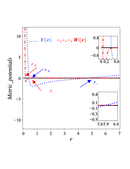
(a)  The metric potential of BH (III.2)

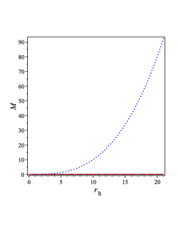
(b)  The metric potential of BH (III.2)

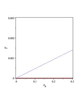
(c)  Hawking temperature of BH (III.2)

Figure 1: Schematic plots of thermodynamic quantities of the black hole solution given by Eq. (III.2): 0(a) the behavior of the metric potentials $V$ and $W$; 0(b) typical behavior of the horizons of the metric potential $V(r)$ given by Eq. (42); 0(c) typical behavior of the horizon temperature given by Eq. (43), showing how the temperature increases with increasing $r_{h}$. All of these values are for $\Lambda_{\mathrm{eff}}=0.02.$

Eq. (37), the Hawking temperature can be calculated as

$$T=\frac{\Lambda_{\mathrm{eff}}r_{h}(5a-2r_{h})}{4\pi(3a-2r_{h})}\,.$$ (43)

The behavior of the Hawking temperature given by Eq. (43) is illustrated in Fig. 1 0(c) which shows that the Hawking temperature is always positive and increasing as $r_{h}$ increases.

Using Eq. (38) we obtain the entropy of the BH (III.2) in the form

$$S=\pi(a+r_{h}{}^{2})\,.$$ (44)

According to Eq. (44), the entropy is different from the usual GR entropy due to the existence of the parameter $a$, when vanishes, we again obtain the usual GR entropy. The difference results from the BH described here having a non-trivial value of the derivative of the function $f(R)$. The behavior of the entropy is shown in Fig. 2 1(a) which indicates that $S$ increases as $r_{h}$ increases.

From Eq. (39), the quasi-local energy takes the form

$$E=\frac{\Lambda_{\mathrm{eff}}[6r_{h}{}^{6}-5r_{h}{}^{4}+35ar_{h}{}^{4}+30a^{2}r_{h}{}^{3}-60ar_{h}{}^{2}-30a^{2}r_{h}\ln(r_{h})+180a^{2}r_{h}{}^{2}+60a^{3}r_{h}\ln(r_{h})-105a^{3}]-5a+5r_{h}{}^{2}}{10r_{h}}\,.$$

The behavior of the quasi–local–energy $E$ is shown in Fig. 2 1(b) which shows that $E$ also increases as $R_{h}$ increases. Using Eq. (40) we obtain the heat capacity of the BH in the form

$$C=\frac{4\pi r_{h}{}^{4}(2r_{h}{}^{2}-5a)}{4r_{h}{}^{4}-8ar_{h}{}^{2}+15a^{2}}\,.$$ (46)

The behavior of the heat capacity is illustrated in Fig. 2 1(c) which shows that $C$ also increases as $r_{h}$ increases.

Finally, we substitute Eqs. (43), (44) and (IV) in Eq. (41) to calculate the Gibbs free energy and obtain

$$G=\frac{1}{20r_{h}(2r_{h}{}^{2}-3a)}\Big{(}\Lambda_{\mathrm{eff}}r_{h}\Big{[}24r_{h}{}^{7}+104ar_{h}{}^{5}-50r_{h}{}^{5}-165ar_{h}{}^{3}+510a^{2}r_{h}{}^{3}+120a^{2}r_{h}{}^{4}-180a^{3}r_{h}{}^{2}+435a^{2}r_{h}$$ (47)

$$-1500a^{3}r_{h}-30\ln(r_{h})\{4a^{2}r_{h}{}^{2}-6a^{3}-8a^{3}r_{h}{}^{2}+12a^{4}-21a^{4}\}\Big{]}+10[3a^{2}+2r_{h}{}^{4}-5ar_{h}{}^{2}]\Big{)}\,.$$

The behavior of this free energy is illustrated in Fig. 2 1(d); $G$ also increases as $r_{h}$ increases.

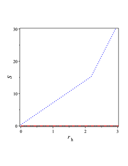
(a)  Entropy of BH (III.2)

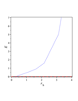
(b)  Quasi local energy of BH (III.2)

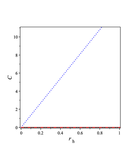
(c)  Heat capacity of BH (III.2)

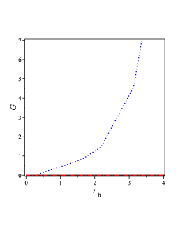
(d)  Gibbs energy of BH (III.2)

Figure 2: Schematic plots of the thermodynamical quantities of the black hole solution given by Eq. (III.2): 1(a) plot of the entropy against the radius horizon showing how the entropy consistently increases as the radius horizon increases; 1(b) typical behavior of the quasi–local energy given by (IV); 1(c) typical behavior of the horizon heat capacity, given by Eq. (40) and 1(d) typical behavior of the Gibb’s free energy given by Eq. (47). The quasi-local energy horizon heat capacity and Gibb’s free energy all increase as $r_{h}$ increase. All of these values are plotted for $\Lambda_{\mathrm{eff}}=0.02$.

It was explained that the use of the thermalon procedure played an important role in the phase transition from AdS to dS Samart and Channuie (2020). Moreover, it is shown that there are big correspondence between Schwarzschild AdS/dS and BH solutions corresponding dual CFTs living on the branes Nojiri and Odintsov (2002). Can the procedures applied in Samart and Channuie (2020); Nojiri and Odintsov (2002) be done on the BHs derived in this study? At present we have no concrete answer. This needs more study which can be done in the future.

IV.1 Application of the first law of thermodynamics to the BHs described by Eq. (III.2)

It is important to check that first law of thermodynamics is valid for the BHs given by Eq. (III.2). Thus, we apply this law to $f(R)$ using the form Zheng and Yang (2018b)

$$dE=TdS-PdV,$$ (48)

where $E$ is the quasi-local energy, $S$ is the Bekenstein–Hawking entropy, $T$ is the hawking temperature, $P$ is the radial component of the stress-energy tensor that serves as the thermodynamic pressure $P=T_{r}{}^{r}\mid_{\pm}$ and $V$ is the geometric volume. Within the framework of $\mathrm{f(R)}$ gravitational theory, the pressure is defined as Zheng and Yang (2018b)

$$P=-\frac{1}{8\pi}\left\{\frac{F}{r_{h}{}^{2}}+\frac{1}{2}(f-RF)\right\}+\frac{1}{4}\left(\frac{2F}{r_{h}}+F^{\prime}\right)T\,.$$ (49)

For the spacetime described by (III.2) if we neglect $O\Big{(}\frac{1}{r^{4}}\Big{)}$ to make the calculations more applicable we get

$$P=-\frac{a+21a^{3}\Lambda_{\mathrm{eff}}-6a^{2}r_{h}\Lambda_{\mathrm{eff}}+12r_{h}a^{3}\Lambda_{\mathrm{eff}}-12ar_{h}{}^{\Lambda}_{\mathrm{eff}}+r_{h}{}^{2}+36a^{2}r_{h}{}^{2}\Lambda_{\mathrm{eff}}+12a^{2}r_{h}{}^{3}\Lambda_{\mathrm{eff}}}{2\,r_{h}{}^{2}}\,.$$ (50)

The derivatives of Eqs. (44) and (IV) are

$$dE=\frac{r_{h}{}^{2}+a+\Lambda_{\mathrm{eff}}[21a^{3}-3r_{h}{}^{4}-12ar_{h}{}^{2}-6a^{2}r_{h}+6r_{h}{}^{6}+21ar_{h}{}^{4}+36a^{2}r_{h}{}^{2}+12a^{2}r_{h}{}^{3}+12a^{3}r_{h}]}{2\,r_{h}{}^{2}}\,,\quad dS=2\pi r_{h}\,.$$

If we substitute Eqs. (43), (50) and (IV.1) in (48) we can show that the first law of thermodynamics aapplies to the BHs.

V Derivation of the stability of the BHs using the geodesic deviation

The path of a test particle in a gravitational field is described by Nashed (2003),

$$\mathit{d^{\mathrm{2}}x^{\sigma}\over d\zeta^{\mathrm{2}}}+\left\{{}^{\sigma}_{\mu\nu}\right\}{dx^{\mu}\over d\zeta}{dx^{\nu}\over d\zeta}=0,$$ (52)

where $\zeta$ is an affine parameter along the geodesic. Equation (52) is the geodesic equation which can be derived as follows D’Inverno (1992),

$$\mathit{{d^{\mathrm{2}}\xi^{\sigma}\over d\zeta^{\mathrm{2}}}+\mathrm{2}\left\{{}^{\sigma}_{\mu\nu}\right\}{dx^{\mu}\over d\zeta}{d\xi^{\nu}\over ds}+\left\{{}^{\sigma}_{\mu\nu}\right\}_{,\ \rho}{dx^{\mu}\over d\zeta}{dx^{\nu}\over d\zeta}\xi^{\rho}=0},$$ (53)

where $\xi^{\rho}$ is the deviation 4-vector. Substituting Eqs. (52) and (53) into Eq. (6) gives

$$\mathit{{d^{\mathrm{2}}t\over d\zeta^{\mathrm{2}}}=0,\qquad{1\over\mathrm{2}}V^{\prime}(r)\left({dt\over d\zeta}\right)^{\mathrm{2}}-r\left({d\phi\over d\zeta}\right)^{\mathrm{2}}=0,\qquad{d^{\mathrm{2}}\theta\over d\zeta^{\mathrm{2}}}=0,\qquad{d^{\mathrm{2}}\phi\over d\zeta^{\mathrm{2}}}=0,}$$ (54)

and for Eq. (53) we get

$$\mathit{{d^{\mathrm{2}}\xi^{\mathrm{1}}\over d\zeta^{\mathrm{2}}}+WV^{\prime}{dt\over d\zeta}{d\xi^{\mathrm{0}}\over d\zeta}-\mathrm{2}rW{d\phi\over d\zeta}{d\xi^{\mathrm{3}}\over d\zeta}+\left[{\mathrm{1}\over\mathrm{2}}\left(V^{\prime}W^{\prime}+W(r)V^{\prime\prime}\right)\left({dt\over d\zeta}\right)^{\mathrm{2}}-\left(W+rW^{\prime}\right)\left({d\phi\over d\zeta}\right)^{\mathrm{2}}\right]\xi^{\mathrm{1}}=0},$$

$$\mathit{{d^{\mathrm{2}}\xi^{\mathrm{0}}\over d\zeta^{\mathrm{2}}}+{V^{\prime}\over V}{dt\over d\zeta}{d\xi^{\mathrm{1}}\over d\zeta}=0,\qquad{d^{\mathrm{2}}\xi^{\mathrm{2}}\over d\zeta^{\mathrm{2}}}+\left({d\phi\over d\zeta}\right)^{\mathrm{2}}\xi^{\mathrm{2}}=0,\qquad\qquad{d^{\mathrm{2}}\xi^{\mathrm{3}}\over d\zeta^{\mathrm{2}}}+{\mathrm{2}\over r}{d\phi\over d\zeta}{d\xi^{\mathrm{1}}\over d\zeta}=0,}$$ (55)

where $V$ and $W$ are defined by Eq. (III.2). Equations (54) and (V) are the geodesic and geodesic deviations of the line–element (6). Using the circular orbit

$$\mathit{\theta={\pi\over\mathrm{2}},\qquad{d\theta\over d\zeta}=0,\qquad{dr\over d\zeta}=0,}$$ (56)

we get

$$\mathit{\left({d\phi\over d\zeta}\right)^{\mathrm{2}}={V^{\prime}\over r(\mathrm{2}V-rV^{\prime})},\qquad\left({dt\over d\zeta}\right)^{\mathrm{2}}={\mathrm{2}\over\mathrm{2}V-rV^{\prime}}.}$$ (57)

Equation (V) can also be written as

$$\mathit{{d^{\mathrm{2}}\xi^{\mathrm{1}}\over d\phi^{\mathrm{2}}}+WV^{\prime}{dt\over d\phi}{d\xi^{\mathrm{0}}\over d\phi}-\mathrm{2}rW{d\xi^{\mathrm{3}}\over d\phi}+\left[{\mathrm{1}\over\mathrm{2}}\left(V^{\prime}W^{\prime}+WV^{\prime\prime}\right)\left({dt\over d\phi}\right)^{\mathrm{2}}-\left(W+rW^{\prime}\right)\right]\zeta^{\mathrm{1}}=0,}$$

$$\mathit{{d^{\mathrm{2}}\xi^{\mathrm{2}}\over d\phi^{\mathrm{2}}}+\xi^{\mathrm{2}}=\mathrm{0},\qquad{d^{\mathrm{2}}\xi^{\mathrm{0}}\over d\phi^{\mathrm{2}}}+{V^{\prime}\over V}{dt\over d\phi}{d\xi^{\mathrm{1}}\over d\phi}=\mathrm{0},\qquad{d^{\mathrm{2}}\xi^{\mathrm{3}}\over d\phi^{\mathrm{2}}}+{\mathrm{2}\over r}{d\xi^{\mathrm{1}}\over d\phi}=\mathrm{0}.}$$ (58)

The second equation in Eq. (V) describes a stable simple harmonic motion. Assuming the solutions to the rest of Eq. (V) to have the form

$$\mathit{\xi^{\mathrm{0}}=\varsigma_{\mathrm{1}}e^{i\omega\phi},\qquad\xi^{\mathrm{1}}=\varsigma_{\mathrm{2}}e^{i\omega\phi},\qquad and\qquad\varsigma^{\mathrm{3}}=\zeta_{\mathrm{3}}e^{i\omega\phi},}$$ (59)

where $\varsigma_{1}$, $\varsigma_{2}$ and $\varsigma_{3}$ are constants and $\phi$ must be determined. From Eqs. (59) and (V) we have

$$\mathit{\displaystyle\frac{\mathrm{3}VWV^{\prime}-\omega^{\mathrm{2}}VV^{\prime}-\mathrm{2}rWV^{\mathrm{{}^{\prime}2}}+rVWV^{\prime\prime}}{VV^{\prime}}>0,}$$ (60)

which is the stability condition. The solution to Eq. (60) has the form

$$\omega^{2}=\mathit{\displaystyle\frac{\mathrm{3}VWV^{\mathrm{{}^{\prime}}}-\mathrm{2}rWV^{\mathrm{{}^{\prime}2}}+rVWV^{\prime\prime}}{VV^{\prime}}>0,}$$ (61)

which is the stability condition for the Eq. (III.2) Misner et al. (1973). Substituting the metric potentials given by Eq. (III.2) in Eq. (61) we can obtain the behavior of the stability condition which is also shown in Fig. 3.

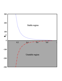
Figure 3: Schematic plot of the stability condition described by Eq. (61)showing the stable and unstable regions.

VI Summary and conclusions

Generally, the field equations of $\mathrm{f(R)}$ are complicated and it is not easy to find an analytical solution. By using the trace of the field equations we can write $\mathrm{f(R)}$ in terms of the remaining terms, i.e., in terms of the derivatives of $\mathrm{f(R)}$ and the  d’Alembertian operator. Using this form of $\mathrm{f(R)}$  we can rewrite  the field equations and apply them to flat horizons using two unknown functions of the radial coordinate. We then derived the differential equations and analyzed them for special cases and derived special cases that coincided with the GR BHs. From this analysis we then derived  general non-trivial BHs that are different from the BHs of GR. These BHs are characterized by a convolution function and depend on a constant that is responsible for making these BHs deviate from GR BHs. In spite of the fact that the field equations do not include a cosmological constant, we obtained solutions that included an effective cosmological constant, this is an advantage of $\mathrm{f(R)}$  gravitational theory. By using  coordinate transformations between the temporal and $\phi$ coordinates we succeeded in deriving new forms of rotating BHs with non-trivial values of the Ricci scalar.

To understand the physics of these BHs we derived the forms of their asymptotes form and showed that they behaved as AdS/dS depending on the sign of the effective cosmological constant. We also showed that such BH solutions coincide with GR BHs when the constant that is associated with the derivative of  $\mathrm{f(R)}$  equals zero. Also, we derived the asymptotic form of $\mathrm{f(R)}$  for these solutions  and showed that it behaves as a polynomial function. To check the singularities of these solutions, we calculated the invariants and showed that the higher–order–curvature terms make the singularities of these BHs softer than those of GR BHs. Thermodynamical quantities such as horizons, Hawking temperature, entropy, heat capacity and Gibbs free energy were also calculated and it was shown that their behavior is consistent with that described in the literature. Moreover, it was demonstrated that these solutions satisfy the first law of thermodynamics. To test the stability of the BHs we used the geodesic deviation and derived the stability condition analytically, the regions of stability were also illustrated graphically. Finally, using odd–type perturbations methods Nashed and Capozziello (2019); Elizalde et al. (2020) we showed that our BHs have no ghosts and that the radial speed has a value of one, which insures that these BHs are stable.

In conclusion we stress that our derived BHs are different from those of GR due to the constant coefficient  in the derivative of  $\mathrm{f(R)}$ which is of order two. Indeed if we change the order of $r$ such that is its coefficient is a constant we derive new BHs that may correspond to a physics completely different  from the BHs presented in this study. This is a topic future study.

References

- Capozziello and Faraoni (2011) S. Capozziello and V. Faraoni, “The landscape beyond einstein gravity,” in Beyond Einstein Gravity: A Survey of Gravitational Theories for Cosmology and Astrophysics (Springer Netherlands, Dordrecht, 2011) pp. 59–106.
- Capozziello and De Laurentis (2011) S. Capozziello and M. De Laurentis, Phys. Rept. 509, 167 (2011), arXiv:1108.6266 [gr-qc] .
- Nojiri and Odintsov (2011) S. Nojiri and S. D. Odintsov, Phys. Rept. 505, 59 (2011), arXiv:1011.0544 [gr-qc] .
- Olmo (2011) G. J. Olmo, Int. J. Mod. Phys. D 20, 413 (2011), arXiv:1101.3864 [gr-qc] .
- Riess et al. (1998) A. G. Riess et al. (Supernova Search Team), Astron. J. 116, 1009 (1998), arXiv:astro-ph/9805201 [astro-ph] .
- Perlmutter et al. (1999) S. Perlmutter et al. (Supernova Cosmology Project), Astrophys. J. 517, 565 (1999), arXiv:astro-ph/9812133 [astro-ph] .
- Riess et al. (2004) A. G. Riess et al. (Supernova Search Team), Astrophys. J. 607, 665 (2004), arXiv:astro-ph/0402512 [astro-ph] .
- Hirata et al. (1987) K. Hirata et al. (Kamiokande-II), GRAND UNIFICATION. PROCEEDINGS, 8TH WORKSHOP, SYRACUSE, USA, APRIL 16-18, 1987, Phys. Rev. Lett. 58, 1490 (1987), [,727(1987)].
- Dodelson and Widrow (1994) S. Dodelson and L. M. Widrow, Phys. Rev. Lett. 72, 17 (1994), arXiv:hep-ph/9303287 [hep-ph] .
- Cole et al. (1994) S. Cole, A. Aragon-Salamanca, C. S. Frenk, J. F. Navarro, and S. E. Zepf, Mon. Not. Roy. Astron. Soc. 271, 781 (1994), arXiv:astro-ph/9402001 [astro-ph] .
- Schmidt (2006) H.-J. Schmidt, eConf C0602061, 12 (2006), arXiv:gr-qc/0602017 .
- Awad et al. (2018) A. Awad, W. El Hanafy, G. G. L. Nashed, S. D. Odintsov, and V. K. Oikonomou, JCAP 07, 026 (2018), arXiv:1710.00682 [gr-qc] .
- Weyl (1919) H. Weyl, Annalen der Physik 364, 101 (1919), https://onlinelibrary.wiley.com/doi/pdf/10.1002/andp.19193641002 .
- Eddington (1988) A. S. Eddington, The Internal Constitution of the Stars, Cambridge Science Classics (Cambridge University Press, 1988).
- Utiyama and DeWitt (1962) R. Utiyama and B. S. DeWitt, Journal of Mathematical Physics 3, 608 (1962).
- Utiyama (1956) R. Utiyama, Phys. Rev. 101, 1597 (1956).
- Buchdahl (1970) H. A. Buchdahl, Monthly Notices of the Royal Astronomical Society 150, 1 (1970), https://academic.oup.com/mnras/article-pdf/150/1/1/8075909/mnras150-0001.pdf .
- Starobinsky (1980) A. A. Starobinsky, Phys. Lett. B91, 99 (1980), [,771(1980)].
- Shah and Samanta (2019) P. Shah and G. C. Samanta, Eur. Phys. J. C79, 414 (2019), arXiv:1905.09051 [gr-qc] .
- Nojiri et al. (2019) S. Nojiri, S. D. Odintsov, and V. K. Oikonomou, Nucl. Phys. B941, 11 (2019), arXiv:1902.03669 [gr-qc] .
- Odintsov and Oikonomou (2019a) S. D. Odintsov and V. K. Oikonomou, Class. Quant. Grav. 36, 065008 (2019a), arXiv:1902.01422 [gr-qc] .
- Odintsov and Oikonomou (2019b) S. D. Odintsov and V. K. Oikonomou, Phys. Rev. D 99, 064049 (2019b).
- Nascimento et al. (2019) J. R. Nascimento, G. J. Olmo, P. J. Porfirio, A. Yu. Petrov, and A. R. Soares, Phys. Rev. D99, 064053 (2019), arXiv:1812.00471 [gr-qc] .
- Miranda et al. (2019) T. Miranda, C. Escamilla-Rivera, O. F. Piattella, and J. C. Fabris, JCAP 1905, 028 (2019), arXiv:1812.01287 [gr-qc] .
- Astashenok et al. (2019) A. V. Astashenok, K. Mosani, S. D. Odintsov, and G. C. Samanta, Int. J. Geom. Meth. Mod. Phys. 16, 1950035 (2019), arXiv:1812.10441 [gr-qc] .
- Elizalde et al. (2019a) E. Elizalde, S. D. Odintsov, T. Paul, and D. S.-C. Gómez, Phys. Rev. D 99, 063506 (2019a).
- Elizalde et al. (2019b) E. Elizalde, S. D. Odintsov, V. K. Oikonomou, and T. Paul, JCAP 1902, 017 (2019b), arXiv:1810.07711 [gr-qc] .
- Chen (2019) L. Chen, Phys. Rev. D 99, 064025 (2019).
- Sbisà et al. (2019) F. Sbisà, O. F. Piattella, and S. E. Jorás, Phys. Rev. D 99, 104046 (2019).
- Bombacigno and Montani (2019) F. Bombacigno and G. Montani, Eur. Phys. J. C79, 405 (2019), arXiv:1809.07563 [gr-qc] .
- Capozziello et al. (2018) S. Capozziello, C. A. Mantica, and L. G. Molinari, Int. J. Geom. Meth. Mod. Phys. 16, 1950008 (2018), arXiv:1810.03204 [gr-qc] .
- Samanta and Godani (2019) G. C. Samanta and N. Godani, Eur. Phys. J. C79, 623 (2019), arXiv:1908.04406 [gr-qc] .
- Multamäki and Vilja (2006) T. Multamäki and I. Vilja, Phys. Rev. D 74, 064022 (2006).
- Nashed (2018a) G. G. L. Nashed, European Physical Journal Plus 133, 18 (2018a).
- Nashed (2018b) G. G. L. Nashed, International Journal of Modern Physics D 27, 1850074 (2018b).
- Nashed (2018) G. G. L. Nashed, Adv. High Energy Phys. 2018, 7323574 (2018).
- De Felice and Tsujikawa (2010) A. De Felice and S. Tsujikawa, Living Rev. Rel. 13, 3 (2010), arXiv:1002.4928 [gr-qc] .
- Moon et al. (2011) T. Moon, Y. S. Myung, and E. J. Son, Gen. Rel. Grav. 43, 3079 (2011), arXiv:1101.1153 [gr-qc] .
- Larranaga (2012) A. Larranaga, Pramana 78, 697 (2012), arXiv:1108.6325 [gr-qc] .
- Cembranos et al. (2014) J. Cembranos, A. de la Cruz-Dombriz, and P. Jimeno Romero, Int. J. Geom. Meth. Mod. Phys. 11, 1450001 (2014), arXiv:1109.4519 [gr-qc] .
- Sheykhi et al. (2014) A. Sheykhi, S. Hendi, and S. Salarpour, Phys. Scripta 10, 105003 (2014).
- Sheykhi (2012a) A. Sheykhi, Gen. Rel. Grav. 44, 2271 (2012a).
- Sawicki and Vikman (2013) I. Sawicki and A. Vikman, Phys. Rev. D 87, 067301 (2013), arXiv:1209.2961 [astro-ph.CO] .
- Cognola et al. (2005) G. Cognola, E. Elizalde, S. Nojiri, S. D. Odintsov, and S. Zerbini, JCAP 02, 010 (2005), arXiv:hep-th/0501096 .
- Sebastiani and Zerbini (2011) L. Sebastiani and S. Zerbini, Eur. Phys. J. C71, 1591 (2011), arXiv:1012.5230 [gr-qc] .
- de la Cruz-Dombriz et al. (2011) A. de la Cruz-Dombriz, A. Dobado, and A. L. Maroto, Phys. Rev. D 83, 029903 (2011).
- Hendi (2010) S. H. Hendi, Phys. Lett. B690, 220 (2010), arXiv:0907.2520 [gr-qc] .
- Hendi et al. (2012) S. H. Hendi, B. Eslam Panah, and S. M. Mousavi, Gen. Rel. Grav. 44, 835 (2012), arXiv:1102.0089 [hep-th] .
- Hendi and Momeni (2011) S. Hendi and D. Momeni, Eur. Phys. J. C 71, 1823 (2011), arXiv:1201.0061 [gr-qc] .
- Mazharimousavi and Halilsoy (2011) S. Mazharimousavi and M. Halilsoy, Phys. Rev. D 84, 064032 (2011), arXiv:1105.3659 [gr-qc] .
- Nojiri and Odintsov (2013) S. Nojiri and S. D. Odintsov, Class. Quant. Grav. 30, 125003 (2013), arXiv:1301.2775 [hep-th] .
- Nojiri and Odintsov (2014) S. Nojiri and S. D. Odintsov, Phys. Lett. B 735, 376 (2014), arXiv:1405.2439 [gr-qc] .
- Banados et al. (1992) M. Banados, C. Teitelboim, and J. Zanelli, Phys. Rev. Lett. 69, 1849 (1992), arXiv:hep-th/9204099 .
- Carroll et al. (2004) S. M. Carroll, V. Duvvuri, M. Trodden, and M. S. Turner, Phys. Rev. D70, 043528 (2004), arXiv:astro-ph/0306438 [astro-ph] .
- Buchdahl (1970) H. A. Buchdahl, mnras 150, 1 (1970).
- Nojiri and Odintsov (2003) S. Nojiri and S. D. Odintsov, Phys. Rev. , 123512 (2003), arXiv:hep-th/0307288 [hep-th] .
- Capozziello et al. (2003) S. Capozziello, V. F. Cardone, S. Carloni, and A. Troisi, Int. J. Mod. Phys. D12, 1969 (2003), arXiv:astro-ph/0307018 [astro-ph] .
- Nojiri et al. (2017) S. Nojiri, S. D. Odintsov, and V. K. Oikonomou, Phys. Rept. 692, 1 (2017), arXiv:1705.11098 [gr-qc] .
- Capozziello (2002) S. Capozziello, Int. J. Mod. Phys. D11, 483 (2002), arXiv:gr-qc/0201033 [gr-qc] .
- Cognola et al. (2005) G. Cognola, E. Elizalde, S. Nojiri, S. D. Odintsov, and S. Zerbini, jcap 2, 010 (2005), hep-th/0501096 .
- Kalita and Mukhopadhyay (2019) S. Kalita and B. Mukhopadhyay, Eur. Phys. J. C79, 877 (2019), arXiv:1910.06564 [gr-qc] .
- Ronveaux (2003) A. Ronveaux, Applied Mathematics and Computation 141, 177 (2003), advanced Special Functions and Related Topics in Differential Equations, Third Melfi Workshop, Proceedings of the Melfi School on Advanced Topics in Mathematics and Physics.
- Maier (2005) R. S. Maier, Journal of Differential Equations 213, 171 (2005).
- Misner et al. (1973) C. W. Misner, K. S. Thorne, and J. A. Wheeler, Gravitation (W. H. Freeman, San Francisco, 1973).
- Klemm et al. (1998) D. Klemm, V. Moretti, and L. Vanzo, Phys. Rev. D57, 6127 (1998), [Erratum: Phys. Rev.D60,109902(1999)], arXiv:gr-qc/9710123 [gr-qc] .
- Lemos (1995) J. P. S. Lemos, Phys. Lett. B353, 46 (1995), arXiv:gr-qc/9404041 [gr-qc] .
- Awad (2003) A. M. Awad, Class. Quant. Grav. 20, 2827 (2003), arXiv:hep-th/0209238 [hep-th] .
- Sheykhi (2012b) A. Sheykhi, Phys. Rev. D 86, 024013 (2012b).
- Sheykhi (2010) A. Sheykhi, Eur. Phys. J. C69, 265 (2010), arXiv:1012.0383 [hep-th] .
- Hendi et al. (2010) S. H. Hendi, A. Sheykhi, and M. H. Dehghani, Eur. Phys. J. C70, 703 (2010), arXiv:1002.0202 [hep-th] .
- Sheykhi et al. (2010) A. Sheykhi, M. H. Dehghani, and S. H. Hendi, Phys. Rev. D 81, 084040 (2010).
- Wang et al. (2019) Y.-Q. Wang, Y.-X. Liu, and S.-W. Wei, Phys. Rev. D99, 064036 (2019), arXiv:1811.08795 [gr-qc] .
- Zakria and Afzal (2018) A. Zakria and A. Afzal, (2018), arXiv:1808.04361 [hep-th] .
- Cognola et al. (2011) G. Cognola, O. Gorbunova, L. Sebastiani, and S. Zerbini, Phys. Rev. D 84, 023515 (2011).
- Zheng and Yang (2018a) Y. Zheng and R.-J. Yang, Eur. Phys. J. C78, 682 (2018a), arXiv:1806.09858 [gr-qc] .
- Kim and Kim (2012) W. Kim and Y. Kim, Phys. Lett. B718, 687 (2012), arXiv:1207.5318 [gr-qc] .
- Nojiri and Odintsov (2017) S. Nojiri and S. D. Odintsov, Phys. Rev. D 96, 104008 (2017), arXiv:1708.05226 [hep-th] .
- Samart and Channuie (2020) D. Samart and P. Channuie, Phys. Rev. D 102, 064008 (2020), arXiv:2001.06096 [gr-qc] .
- Nojiri and Odintsov (2002) S. Nojiri and S. D. Odintsov, Phys. Rev. D 66, 044012 (2002), arXiv:hep-th/0204112 .
- Zheng and Yang (2018b) Y. Zheng and R. Yang, The European Physical Journal C 78 (2018b), 10.1140/epjc/s10052-018-6167-4.
- Nashed (2003) G. G. L. Nashed, Chaos Solitons Fractals 15, 841 (2003), arXiv:gr-qc/0301008 .
- D’Inverno (1992) R. A. D’Inverno, Internationale Elektronische Rundschau (1992).
- Nashed and Capozziello (2019) G. G. L. Nashed and S. Capozziello, Phys. Rev. D99, 104018 (2019), arXiv:1902.06783 [gr-qc] .
- Elizalde et al. (2020) E. Elizalde, G. G. L. Nashed, S. Nojiri, and S. D. Odintsov, Eur. Phys. J. C80, 109 (2020), arXiv:2001.11357 [gr-qc] .