Using a deep neural network to predict the motion of under-resolved triangular rigid bodies in an incompressible flow

Abstract

We consider non-spherical rigid body particles in an incompressible fluid in the regime where the particles are too large to assume that they are simply transported with the fluid without back-coupling and where the particles are also too small to make fully resolved direct numerical simulations feasible. Unfitted finite element methods with ghost-penalty stabilisation are well suited to fluid-structure-interaction problems as posed by this setting, due to the flexible and accurate geometry handling and for allowing topology changes in the geometry. In the computationally under resolved setting posed here, accurate computations of the forces by their boundary integral formulation are not viable. Furthermore, analytical laws are not available due to the shape of the particles. However, accurate values of the forces are essential for realistic motion of the particles. To obtain these forces accurately, we train an artificial deep neural network using data from prototypical resolved simulations. This network is then able to predict the force values based on information which can be obtained accurately in an under-resolved setting. As a result, we obtain forces on very coarse and under-resolved meshes which are on average an order of magnitude more accurate compared to the direct boundary-integral computation from the Navier-Stokes solution, leading to solid motion comparable to that obtained on highly resolved meshes that would substantially increase the simulation costs.

1 Introduction

The aim of this work is to simulate multiple small triangular rigid bodies inside an incompressible fluid using a moving domain approach [1, 2, 3], within an unfitted finite element method known as CutFEM [4]. Solids in flows are the subject of various applications in engineering and medicine. The homogenised behaviour of these particles is well studied, but numerical simulations on the fine scale, considering resolved particles are rare, especially when non-spherical bodies are considered.

If the solid particles within the fluid are very small, they can be considered as point-like within the flow field and the interaction can be represented in a discrete element framework in terms of analytical laws for the fluid mechanical coefficients, as well as by modelling the effect of the bodies on the surrounding flow. Approximative laws exist for some simple shaped non-spherical particles [5, 6, 7, 8, 9] and simulations with a very large number of particles can be realised in mixed continuum mechanics / discrete element frameworks.

However, if the particles are assumed to be large, only a resolved simulation remains. When considering spherical particles, Arbitrary Lagrangian Eulerian (ALE) approaches can be used. These allow for very good accuracy on relatively coarse grids [10, 11]. The ALE method is based on fixed reference domains that allow to resolve the boundaries of the particles exactly. The motion of the particles is implicitly tracked by mapping the flow problem onto this reference domain. ALE approaches are highly efficient and accurate but whenever the motion (or rotation) of the particles gets too large, they suffer from a distortion of the underlying finite element mesh and call for remeshing. This approach is highly efficient and very well established in the area of elastic fluid structure interactions [12, 13, 14]. However, if a very large number of particles are considered, or if they are no longer radially symmetric, alternative discretisation methods must be considered as tracking the single particles with a finite element mesh may require a prohibitive computational effort. A prominent example is the immersed boundary method, going back to Peskin [15], which is able to efficiently simulate dense particle suspensions [16]. Although the particles must not be exactly resolved, these methods still require an increased mesh resolution in the vicinity of the particles.

Finally, we note that on a theoretical level, the motion of rigid bodies of arbitrary shapes has been studied by Brenner and summarised by Happel and Brenner in [17]. However, these considerations only take into account the case of creeping flows governed by the linear Stokes equations, rather than the full non-linear Navier-Stokes equations considered here.

In this work we define a hybrid finite element / (deep) neural network framework that allows us to describe the interaction with rigid bodies of triangular shape on under-resolved meshes accurately. Triangular bodies are a simple example of non-spherical shapes where no rotational symmetry can be assumed that would allow us to use efficient and accurate ALE approaches. Furthermore, since triangles involve re-entrant corners, the approximation property of the finite element solution suffers, which poses another challenge to the coupled simulation. Both problems also arise for general polygonal objects, but by choosing triangles we can restrict ourselves to geometries that are easy to parametrise in this demonstration. In order to write the transfer of forces between flow and particles with sufficient accuracy, we will use a neural network that represents the forces acting on a particle as a function of the particular flow situation instead of directly evaluating the forces from the Navier-Stokes solution. This network is trained in a presented offline phase based on prototypical resolved simulations. A similar approach with non-spherical but very small particles in the linear Stokes regime has recently been described by Minakowska et al. [18]. In principle this procedure can be transferred to all interface capturing schemes that allow for a robust under-resolved representation of structures in a background mesh. Besides different CutFEM or extended finite element approaches [19, 20, 21, 4] locally adjusted or parametric finite element methods [22, 23, 24] are also an option.

Finally, we will illustrate that our neural network approach can efficiently represent the interaction of a fluid with non-spherical particles with high accuracy on coarse grids. To date, there is no efficient alternative approach. ALE methods are too costly due the the constant need for remeshing and resolved CutFEM approaches are not competitive for their limited approximation properties that would require highly refined meshes at the particles.

Example 1 (Motivation of approach).

The approach is based in the hypothesis that while it may not be possible to evaluate transmission forces with sufficient accuracy on coarse and efficient discretisations, averaged flow features can indeed be obtained obtained accurately on such meshes and that these features are sufficient to predict the transmission forces with help of a neural network. To illustrate that we can accurately compute volumetric flow features accurately, while the boundary forces are not computed accurately in an under-resolved CutFEM simulations, we consider the well-established benchmark flow around a cylinder [25], where the laminar flow around a cylinder is considered and where the forces on the cylinder are taken as goal values for a quantitative evaluation of different discretisations, see Figure 1 for a sketch of the solution. We note that the configuration is slightly non-symmetric with the cylinder not being vertically centred such that a non-vanishing lift coefficient will result. Here we take the stationary "2D-1" test case and compute this once using a fitted approach together with the Babuška-Miller trick [26] to evaluate the drag and lift functional, and once using a CutFEM approach [27, 28] together with an isoparametric mapping approach [29, 30] to obtain the necessary geometry approximation of the discrete level set domain but with the direct evaluation of the boundary integral to realise the force values. For both the fitted and unfitted simulations we use inf-sup stable Taylor-Hood elements $\mathbb{P}^{k}/\mathbb{P}^{k-1}$, which we shall abbreviate as $\texttt{TH}_{k}$. For the present computations we take the order $k=3$. To make the comparison as fair as possible, we consider unstructured meshes with the same mesh size in each computation.

These and all following numerical finite element computations are implemented using the finite element library NGSolve/netgen [31, 32]. For CutFEM computations, we additionally use the add-on ngsxfem [33] for unfitted finite element functionality within the NGSolve framework.

In Figure 1 we can see the velocity solution to these computations together with the computational meshes. Note that it is nearly impossible to distinguish the two solutions visually. In Table 1 we see the benchmark quantities resulting from the two computations. Here we immediately see that while the values from the fitted computations are reasonably for such coarse meshes, the values resulting from the CutFEM computations even result in the wrong sign for the lift coefficient.

Since the solution in the bulk of the domains look so indistinguishable, it is natural to ask, whether there are other quantities based on the solution near the obstacle, which we can compute accurately in both settings. To this end, we compute the average velocity in a strip of width $0.05$ around the obstacle. The results from this are presented in Table 2. Here we see that while the fitted FEM solution resulted in values closer to the reference values compared to CutFEM, the difference between the accuracy of the fitted and unfitted computations are significantly smaller. Furthermore we see that we keep multiple significant figures of accuracy in the functional value, even at values of order $10^{-5}$.

We conclude from this, that while it is difficult to obtain accurate forces from the boundary integral formulation in an under-resolved CutFEM computation, other features of the solution can be obtained much more accurately even on such coarse meshes. Therefore, if we are able to construct a mapping from flow features near the obstacle to the forces acting on the obstacle, we should be able to get more accurate force values in the under resolved CutFEM setting.

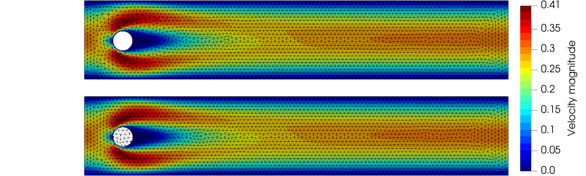
Figure 1: Velocity solution to the ST-2D1 problem with $h_{max}=0.02$. Top: Fitted FEM, bottom: CutFEM.

Method	$c_{\text{drag}}$	(err)	$c_{\text{lift}}$	(err)	$\Delta p$	(err)
Fitted $\texttt{TH}_{3}$	5.579521	0.00025%	$0.0105942$	0.232%	0.117162	0.3046%
CutFEM $\texttt{TH}_{3}$	5.571512	0.14379%	$-0.0063662$	160.0%	0.119766	1.9111%
Ref.	5.579535	–	0.0106189	–	0.117520	–

Table 1: Benchmark quantities for the ST-2D1 problem computed using fitted FEM and CutFEM on meshes with $h_{max}=0.02$. Reference values obtained from www.featflow.de (accessed on 15th Feb. 2021).

Method	Avg. $\bm{u}_{1}$	(err)	Avg. $\bm{u}_{2}$	(err)
Fitted $\texttt{TH}_{3}$	$0.004\,293\,270\,580\,011$	0.0013%	$1.492\,002\,457\,785\,17\text{\cdot}{10}^{-05}$	0.0306%
CutFEM $\texttt{TH}_{3}$	$0.004\,287\,956\,263\,878$	1.2506%	$1.493\,165\,046\,467\,2\text{\cdot}{10}^{-05}$	0.1086%
Ref.	$0.004\,293\,325\,595\,639\,2$	–	$1.491\,545\,422\,670\,73\text{\cdot}{10}^{-05}$	–

Table 2: Average velocity in a strip of width 0.05 around the obstacle. Reference values computed using a fitted approach with $\texttt{TH}_{6}$ elements on a mesh with $h_{max}=0.005$. We also indicate the relative error of both approaches compared to the reference solution.

The remainder of this text is structured as follows. In the following section 2 we describe the basic equations governing the system of a rigid body in an incompressible fluid. In subsection 2.1 we then discuss the relevant physical parameters we will consider. Section 3 covers the details of the neural network, that is the design, the generation of the training data and the results of the training. Furthermore, we validate the accuracy of the network prediction in comparison to the direct evaluation from the Navier-Stokes solution in the setting of the generated training data. In section 4 we will then apply the resulting network in different scenarios, in order to compare the results against a resolved ALE solution and to show the capabilities of the method in settings where a standard ALE discretisation is not realisable. In section 5 we give some concluding remarks.

2 Governing equations

Let us consider an open bounded domain $\Omega=\pazocal{F}\>\dot{\cup}\>\pazocal{I}\>\dot{\cup}\>\pazocal{S}\subset\mathds{R}^{d}$, $d\in\{2,3\}$, divided into a $d$-dimensional fluid region $\pazocal{F}$, a $d$-dimensional solid region $\pazocal{S}$ and a $d-1$-dimensional interface region $\pazocal{I}$ coupling the two. The fluid in $\pazocal{F}$ is governed by the incompressible Navier-Stokes equations: Find a velocity and pressure $(\bm{u},p)$ such that

$$\rho{F}\left(\partial_{t}\bm{u}+(\bm{u}\cdot\nabla)\bm{u}\right)-\operatorname{div}\bm{\sigma}(\bm{u},p) =\rho{F}\bm{f}$$ (2.1)

$$\operatorname{div}(\bm{u}) =0$$

holds in $\pazocal{F}$ with a given fluid density $\rho{F}$, an external body force $\bm{f}$ and the Cauchy stress tensor

$$\bm{\sigma}(\bm{u},p)=\mu{F}(\nabla\bm{u}+\nabla\bm{u}^{T})-\operatorname{Id}p$$

where $\operatorname{Id}$ is the identity tensor, $\mu{F}=\rho{F}\nu_{f}$ is the fluid’s dynamic viscosity and $\nu{F}$ the kinematic viscosity. The boundary conditions which complete the system (2.1) will be given later. We shall consider the homogeneous form of (2.1), i.e., we take $\bm{f}\equiv 0$.

We further divide the solid region $\pazocal{S}=\dot{\bigcup}_{i=1}^{N}\pazocal{B}_{i}$ into a finite set of distinct rigid bodies (particles) $\pazocal{B}_{i}$. For simplicity, we assume that they each have the same homogeneous density $\rho{S}$. Let

$$U_{i}^{\text{total}}=U_{i}+\bm{\omega}_{i}\times\bm{r}$$

be the motion of $\pazocal{B}_{i}$, where $U_{i}$ is the particle’s velocity, $\bm{\omega}_{i}$ it’s angular velocity and $\bm{r}=\bm{x}-c{B}$ the position vector of a point in $\overline{\pazocal{B}}_{i}$ relative to the body’s centroid $c{B}$. These two velocities are then governed by the Newton-Euler equations

$$m{B}\partial_{t}U_{i} =\bm{F}+\bm{F}_{\text{buoyant}}+\bm{F}_{\text{gravity}}$$ (2.2a)

$$\bm{I}{B}\partial_{t}\bm{\omega}+\bm{\omega}\times\bm{I}{B}\bm{\omega} =\bm{T}+\bm{T}_{\text{buoyant}}$$ (2.2b)

with the particles mass $m{B}=\rho{S}\operatorname{vol}(\pazocal{B})$, the force and torque exerted by the fluid on the particle

$$\bm{F}=\int_{\partial\pazocal{B}_{i}}\bm{\sigma}(\bm{u},p)\bm{n}\operatorname{d\!}S\qquad\text{and}\qquad\bm{T}=\int_{\partial\pazocal{B}_{i}}\bm{r}\times\bm{\sigma}(\bm{u},p)\bm{n}\operatorname{d\!}S$$

and the particles moment of inertia tensor defined by

$$\bm{I}{B}=\rho{S}\int_{\pazocal{B}_{i}}(\|\bm{r}\|^{2}\operatorname{Id}_{3}-\bm{r}\otimes\bm{r})\operatorname{d\!}\bm{x}.$$

The buoyancy force and torque are

$$\bm{F}_{\text{buoyant}}=-m{F}\bm{g}\quad\text{and}\quad\bm{T}_{\text{buoyant}}=-m{F}\bm{r}_{bo}\times\bm{g}$$

where $m{F}=\rho{F}\operatorname{vol}(\pazocal{B}_{i})$ is the mass of the displaced fluid and $\bm{r}_{bo}$ is the vector from the centre of mass to the centre of buoyancy. The centre of buoyancy is defined as the centroid of the displaced fluid volume. Since the particles are completely submersed and both the fluid and solid have a constant density, the centre of mass and centre of buoyancy coincide, such that $\bm{r}_{bo}=0$ and therefore $\bm{T}_{\text{buoyant}}=0$. Note that equivalently, the buoyancy effects can be included in the system by including the forces due to gravity on the right hand side of (2.1). However, since we do not consider pressure-robust discretisations [34] here, including buoyancy in the solid and ignoring gravity on the fluid is more accurate on the discrete level. Finally, the pull due to gravity is

$$\bm{F}_{\text{gravity}}=m{S}\bm{g}.$$

To complete the system (2.1) we need to impose boundary conditions. We shall consider $\Omega$ as a closed aquarium, and therefore take the no-slip boundary conditions

$$\bm{u}=\bm{0}\text{ on }\partial\Omega\qquad\text{and}\qquad\bm{u}=U_{i}^{\text{total}}\text{ on }\partial\pazocal{B}_{i}$$ (2.3)

which couples the fluid and solid equations. The complete system is then defined as the solution to (2.1), (2.2) and (2.3). The pressure is uniquely defined by taking $p\in\pazocal{L}^{2}_{0}(\pazocal{F})$.

Remark.

We note that in two spatial dimensions, the quadratic term $\bm{\omega}\times\bm{I}{B}\bm{\omega}$ vanishes in (2.2b) and the moment of inertia reduces to the scalar $I{B}=\rho{S}\int{B}\|\bm{r}\|^{2}\operatorname{d\!}\bm{x}.$

2.1 Choice of parameters

We choose our fluid and solid material parameters, in order to have a setting which can be given some physical meaning while remaining at small to moderate Reynolds numbers.

The fluid and solid parameters are chosen to approximate coarse sand in a glycerol/water mixture. We take a mixture of 1 part water to 4 parts glycerol at a temperature of $21\unit{}$. The resulting relevant material parameters are summarised in Table 3. The fluid parameters are obtained through an online calculator tool and the density of the solid is taken as the density of quartz. The ISO standard 14688-1:2017 defines coarse sand to have a particle size of 0.63 – 2.0 $\mathrm{mm}$. We therefore take the side length of our triangles to be $d{B}=$2\text{\cdot}{10}^{-3}\text{\,}\mathrm{m}$$.

Parameter	$\mu{F}$	$\rho{F}$	$\nu{F}$	$\rho{S}$
Value	$0.085\,679\text{\,}\mathrm{N}\text{\,}\mathrm{s}\text{\,}{\mathrm{m}}^{-2}$	$1216.7\text{\,}\mathrm{kg}\text{\,}{\mathrm{m}}^{-3}$	$0.000\,070\,419\text{\,}{\mathrm{m}}^{2}\text{\,}{\mathrm{s}}^{-1}$	$2650\text{\,}\mathrm{kg}\text{\,}{\mathrm{m}}^{-3}$

Table 3: Fluid and solid material properties of a 1:4 water-glycerine mixture and quartz

With these parameters, we have established the terminal settling velocity of a particle without rotational or horizontal motion to be $v=0.047$\mathrm{m}\text{\,}{\mathrm{s}}^{-1}$$, c.f. subsubsection 3.2.1. Taking the side-length of the triangular particle as the reference length, this leads to a Reynolds number of $Re=\frac{vL}{\nu{F}}\approx 1.33$. This is sufficiently large to justify considering the full Navier-Stokes equations, rather than the creeping flow Stokes equations, and small enough to ensure that the local flow around the triangle is not turbulent.

3 Neural Network

As we have discussed above, our aim is to train a (deep) neural network which predicts the forces acting on a small triangular rigid body, based on information retrieved from the fluid solution within the bulk of the fluid near the obstacle. In principle this should be possible, for example Raissi et. al. [35] where able to reproduce the Navier-Stokes solution from images using a physics informed neural network [36] or Minakowska et. al. [18] used a very simple deep neural network to predict the forces acting on blood platelets of different shapes in a Stokes flow.

3.1 Network design

As the work in [18] is relatively similar with respect to the aim we have here, we shall take this as our reference point for the design of our network. We note that while in [18] it was the aim to use a neural network to predict the forces based on the speed and shape of very small particle in a linear Stokes flow and without back-coupling of the particles onto the fluid, we want to predict the forces based on the fluid solution near our particle which couples back to the fluid which is governed by the non-linear Navier-Stokes equations.

3.1.1 Network Input

The first question we have to consider is the choice of flow features to feed into the network. To capture the force acting on the triangular rigid body, it makes sense that the features have to be in some sense local to the rigid body. Point evaluations of the velocity and pressure near the rigid body would be one choice. Unfortunately, while we found that this does indeed capture the necessary information needed by a neural network, the unresolved nature of the CutFEM discretisation means that we do not have a chance of obtaining sufficiently accurate values to feed to the network at run-time.

As we have seen in 1, an integral of the velocity components, can be obtained accurately in a coarse CutFEM computation. For a rigid body $\pazocal{B}$, we define $\pazocal{O}(\pazocal{B})\coloneqq\{\bm{x}\in\pazocal{F}\;|\;\|\bm{x}-c{B}\|_{2}^{2}<(d{O}/2)^{2}\}$ to be a circular fluid domain around the solid, centred at the solid’s centre of mass with radius $d{S}$. As the network input, we then take the mean fluid velocity, relative to the solids velocity in $\pazocal{O}(\pazocal{B})$, i.e,

$$\textbf{rel vel}\coloneqq\int_{\pazocal{O}(\pazocal{B})}\bm{u}-U^{\text{total}}\operatorname{d\!}\bm{x}.$$

We have found $d{O}=4d{B}$ to be an appropriate choice. For the input we then de-dimensionalise the data and take $\textbf{input}=\textbf{rel vel}/v$, where $v$ is the characteristic velocity, which we take as the terminal settling velocity $v=0.047$\mathrm{m}\text{\,}{\mathrm{s}}^{-1}$$.

Assuming that the mesh size is not coarser than the size of the triangular rigid body, we can then safely apply the isoparametric mapping technique [29, 30] to accurately integrate over this domain in the CutFEM setting, without distorting the three level sets describing the sides of the triangular body.

As the forces only depend on the angle of attack between the mean (integrated) flow relative to the triangles velocity and the orientation of the triangle, we shall consider the input in a reference configuration. For this we choose the bottom side of the triangle to be parallel to the $x$-axis. As a result, the network learns the forces resulting from any angle of attack in this reference orientation. To obtain the physical forces, we therefore rotate the input into the reference configuration and rotate the drag/lift predictions back into the physical orientation. We also refer to Figure 3 for a sketch of this configuration. Since the torque in two spatial dimensions is a scalar quantity, it is invariant with respect to rotation.

3.1.2 Network output

To keep the network general, we train the network to learn the dimensionless drag, lift and torque coefficients

$$C_{\text{drag}}=\frac{2}{v^{2}\rho{F}L}\bm{F}_{1},\qquad C_{\text{lift}}=\frac{2}{v^{2}\rho{F}L}\bm{F}_{2}\qquad\text{and}\qquad C_{\text{torque}}=\frac{4}{v^{2}\rho{F}L^{2}}\bm{T}.$$

The reference speed is taken as the terminal velocity established below as $v=0.047$\mathrm{m}\text{\,}{\mathrm{s}}^{-1}$$ and the reference length $L=d{S}=0.002$\mathrm{m}$$.

3.1.3 Network architecture

We shall consider a fully connected feed-forward network with at least three hidden layers and the ReLU activation function, i.e., $f(x)=\max\{0,x\}$. An example of such a network can be seen in Figure 2. We shall refer to networks by the number of neurones. For example, with $l_{1}/l_{2}/l_{3}$ we denote a network with three hidden layers consisting of $l_{1}$, $l_{2}$ and $l_{3}$ neurones respectively. The number of neurones per layer and the number of layers we shall need for our network will be determined experimentally, by inspecting the results achieved during training. See subsection 3.3 below.

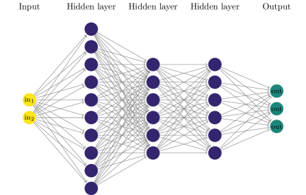
Figure 2: Illustration of a fully connected feed-forward network with two inputs, three hidden layers consisting of 10, 6, and 6 neurones respectively and a three outputs.

3.2 Training Data

In order to train a network, we need to generate the appropriate input and target data.

3.2.1 A priori computations

Neural networks are generally only accurate if they are applied in scenarios which lie in the data range with which the network was trained. We therefore need some information on how fast a triangular rigid body will fall under the acceleration due to gravity as described in section 2 with the material parameters described in subsection 2.1.

To get a better sense of the speeds with which we need to generate the training data with, we consider an ALE discretisation of a single triangular rigid body falling without rotation in a viscous fluid. To this end we consider the domain $\Omega=(0,0.1)\times(0,0.2)$ and a triangular particle of side-length $0.002$ with the centroid $(0.05,0.15)$ at $t=0$. For the fluid and solid parameters we take the parameters described in Table 3. We then solve a simplified (restricted to vertical motion) form of the system (2.1), (2.2) and (2.3) until $t=10$. To solve the coupled fluid-solid problem, we consider a partitioned approach, i.e., we solve the fluid and solid problem separately and iterate between the two until the system is solved implicitly, see section 4 below and [11].To make the ALE mapping simple, we only allow motion in the vertical direction, i.e., we ignore the effects of horizontal drag and torque. For the construction of such a mapping we refer to [11]. We consider this set up for 10 different angles of attack of the triangle and evaluate the terminal velocity.

For this computation we use a mesh with $h_{max}=$1\text{\cdot}{10}^{-3}$$ in the bulk and $h_{max}=$2.5\text{\cdot}{10}^{-4}$$ on the triangle boundary with $\mathbb{P}_{5}/\mathbb{P}_{3}^{dc}$ finite elements, resulting in a FE space with $\texttt{dof}=$211\,658$$ and $\texttt{dof}_{\texttt{cond}}=$84\,230$$. The time-derivative and mesh velocity are approximated using the BDF1 scheme and the time-step used is $\Delta t=\nicefrac{{1}}{{500}}$.

In the resulting computations, we observed that the maximal terminal velocity of the triangle was $0.047$\mathrm{m}\text{\,}{\mathrm{s}}^{-1}$$. This gives us a good indication for the maximal velocity we need to consider to generate training data with.

3.2.2 Generating training data

In order to create a network of which we can expect sufficient accuracy, we generate the training data in a setting which is as close to the application as possible. However, in contrast to the following application of the network, where as coarse as possible discretisations are used for efficient simulations, training data is obtained on highly resolved meshes.

Set-up: Translational motion

To generate learning data for translational motion, we take the domain $(0,0.5)^{2}$ with the equilateral triangular obstacle located at $(0.25,0.25)$ in the reference configuration. This rigid body is then moved from $(0.1,0.25)$ to $(0.4,0.25)$ and back again over a time interval $[0,t_{end}]$. To get a wide range of relative velocities between the triangle and the mean flow around the triangle, we accelerate the particle at different rates, i.e., consider different values for $t_{end}$. The physical location of the body is then given by

$$(0.25-0.15\cos\big{(}\frac{\pi t}{2t_{end}}\big{)},0.25).$$

for $t\in[0,t_{end}]$. To implement this motion, we use a prescribed ALE mapping, as above. In order to generate the data with different angles of attack, we rotate the rigid body by an angle $\alpha$ around it’s centre of mass and rotate the resulting relative velocities and forces back into the reference configuration. As a result, we can reuse the same ALE mapping to simulate different directions of relative motion of the solid body. A sketch of this configuration in the ALE reference configuration can be seen in Figure 3.

Set-up: Rotational motion

Since the above ALE computations only include translational motion, this is equivalent to only considering a parallel flow around a fixed obstacle. For the network to be universally usable, we therefore also need to include rotational flow data. This corresponds to rotating the triangle. To this end, we consider a triangular rigid body located at the centre of the domain $\Omega=(0,0.1)^{2}$. This is then rotated at different speeds, clockwise and anti-clockwise, such that the total rotation at time $t$ with respect to the initial configuration is given by $\sin(2\pi\cdot t/t_{end})$.

In this situation, using ALE is not suitable, as relatively small rotations will lead to mesh-entanglement. We therefore use a highly resolved moving domain CutFEM simulation, to generate data with rotational input. Further details of this method are given below in section 4.

Figure 3: Sketch of the computational domain to generate the learning data set.

Validation

In order to ensure that the generated learning data is computed sufficiently accurate, we consider the above cases over a series of meshes and time-steps. For this test case, we take $t_{end}=2.0$ for both set-ups and $\alpha=0$ for the translational set-up.

For the ALE discretisation, we take $\texttt{TH}_{4}$ elements on a mesh with diameter $h_{max}$ in the bulk and a local mesh parameter $h_{loc}$ on the boundary of the rigid body. In time we discretise using the BDF1 scheme with the time-step $\Delta t$.

For the CutFEM discretisation, we take $\texttt{TH}_{2}$ elements on a mesh with global meshing parameter $h_{max}$ and performing 3 levels of mesh bisections in the domain where we compute the average relative velocity with an additional 5 levels of mesh bisections in the bounding circle of the rotating triangle.

The results for the convergence study can be seen in Table 4. For the ALE computations, we see that the discretisation is accurate and that the second mesh already provides 2 – 3 significant figures of accuracy in the target data. Since the neural network prediction will introduce an additional approximation error, we consider this to be sufficiently accurate for the training data. For the rotational CutFEM data, we see that the forces are (in absolute value) significantly smaller than the translational data. However we also see, that the second finest discretisation should be accurate enough for the training of the network.

Case(Method)	$h_{max}$	$h_{loc}$	$\Delta t$	$C_{\text{drag},\text{max}}$	$C_{\text{lift},\text{min}}$	$C_{\text{torque},\text{max}}$
Translational (ALE)	0.02	$2\cdot 10^{-4}$	$\nicefrac{{1}}{{250}}$	$2.6094\text{\cdot}{10}^{02}$	$-5.9548\text{\cdot}{10}^{01}$	$2.9674\text{\cdot}{10}^{01}$
	0.01	$1\cdot 10^{-4}$	$\nicefrac{{1}}{{500}}$	$2.6105\text{\cdot}{10}^{02}$	$-5.9673\text{\cdot}{10}^{01}$	$2.9699\text{\cdot}{10}^{01}$
	0.005	$5\cdot 10^{-5}$	$\nicefrac{{1}}{{1000}}$	$2.6111\text{\cdot}{10}^{02}$	$-5.9751\text{\cdot}{10}^{01}$	$2.9694\text{\cdot}{10}^{01}$
Rotational: (CutFEM)	0.0084	–	$\nicefrac{{1}}{{250}}$	$1.6025\text{\cdot}{10}^{-02}$	$-1.3880\text{\cdot}{10}^{-02}$	$3.3697\text{\cdot}{10}^{-01}$
	0.0042	–	$\nicefrac{{1}}{{500}}$	$1.3443\text{\cdot}{10}^{-02}$	$-1.5876\text{\cdot}{10}^{-02}$	$3.5969\text{\cdot}{10}^{-01}$
	0.0021	–	$\nicefrac{{1}}{{1000}}$	$1.0735\text{\cdot}{10}^{-02}$	$-8.9824\text{\cdot}{10}^{-03}$	$3.5636\text{\cdot}{10}^{-01}$

Table 4: Validation results of the discretisation to generate the training data set.

Remark.

It is known, that in general, the (fully) implicit BDF1 method is not a good choice to discretise the time-derivative in the Navier-Stokes equations, since the scheme is too diffusive, thus preventing for example vortex shedding. However, the choice of BDF1 here is not problematic, since we are considering flows with small Reynolds numbers. Furthermore, we have tested computations with the less diffusive BDF2 scheme and no significant differences could be observed in the solution.

Generation

To generate the data set, we consider $t_{end}\in\{2,2.5,3,4,6,8,1\}$ and rotate the triangle with angle $\alpha\in\{\frac{2i\pi}{3\cdot 40}\;|\;i=0,\dots,39\}$. Since the triangle is equilateral, the remaining angles of attack $\alpha\in[\nicefrac{{2\pi}}{{3}},2\pi)$ can be obtained by post-processing the data appropriately. Based on the above validation computations, we consider the mesh with $h_{max}=0.01$ and take the time-step $\Delta t=\nicefrac{{1}}{{500}}$.

The resulting data set then contains $2\,130\,000$ input/output pairs.

For the rotational data we choose $t_{end}\in\{0.5,1,2,3,5,6\}$. Again, from the above computations, we take the mesh with $h_{max}=0.0042$ and the time-step is chosen as $\Delta t=\nicefrac{{1}}{{500}}$. As a result, we then obtain an additional $8792$ data sets.

3.3 Training

We implement the neural network described in subsection 3.1 using PyTorch [37]. We use the mean squared error as the loss function and take the Adam algorithm as the optimiser with a step size of $10^{-4}$. The network is trained for a total of 20000 epochs. For the network to be able to predict all three values at the same time, we scale both the input and output data to be in the interval $[-1,1]$. In practice, the predictions are then scaled back appropriately, so that the appropriate coefficients are obtained.

To ensure that the we do not over-fit the network to the training data set, we additionally generated a validation data set in the same fashion as the translational part of the training data set but with different angles of attack and values for $t_{end}$ This then consists of $431\,766$ data points. During training we then also evaluate the network on the validation data set and ensure that the the training error does not decrease while the validation error increases.

The errors of the predictions made by the networks on the training and validation data sets can be seen in Table 5 for the case where a single network was used to predict drag lift and torque, while Table 6 shows the error for separate networks for each force. To make the results on data sets of different sizes comparable, we use the norm $\|\text{err}\|_{mean}^{2}\coloneqq\frac{1}{N}\sum_{i=1}^{N}(\text{prediction}_{i}-\text{value}_{i})^{2}$ and $\|\text{err}\|_{\infty}=\max_{i=1,\dots,N}(|\text{prediction}_{i}-\text{value}_{i}|)$.

To find an appropriate network size, which is large enough to capture all the information contained in the data set, while also being small enough for fast evaluations in the final solver, we consider a number of different networks. The chosen number of layers and neurones per layer can be seen in the first column of Table 5.

			Training data		Validation data
Architecture	Parameters	Target	$\|\cdot\|_{mean}$	$\|\cdot\|_{\infty}$	$\|\cdot\|_{mean}$	$\|\cdot\|_{\infty}$
30/20/10	953	$C_{\text{drag}}$	$1.658\text{\cdot}{10}^{00}$	$1.726\text{\cdot}{10}^{01}$	$1.867\text{\cdot}{10}^{00}$	$1.191\text{\cdot}{10}^{01}$
		$C_{\text{lift}}$	$1.640\text{\cdot}{10}^{00}$	$1.883\text{\cdot}{10}^{01}$	$1.773\text{\cdot}{10}^{00}$	$1.460\text{\cdot}{10}^{01}$
		$C_{\text{torque}}$	$5.872\text{\cdot}{10}^{-01}$	$5.006\text{\cdot}{10}^{00}$	$6.573\text{\cdot}{10}^{-01}$	$4.293\text{\cdot}{10}^{00}$
50/20/20	1653	$C_{\text{drag}}$	$1.047\text{\cdot}{10}^{00}$	$8.618\text{\cdot}{10}^{00}$	$1.186\text{\cdot}{10}^{00}$	$7.876\text{\cdot}{10}^{00}$
		$C_{\text{lift}}$	$1.048\text{\cdot}{10}^{00}$	$8.918\text{\cdot}{10}^{00}$	$1.174\text{\cdot}{10}^{00}$	$8.123\text{\cdot}{10}^{00}$
		$C_{\text{torque}}$	$5.560\text{\cdot}{10}^{-01}$	$4.160\text{\cdot}{10}^{00}$	$6.253\text{\cdot}{10}^{-01}$	$3.746\text{\cdot}{10}^{00}$
50/20/20/10	1833	$C_{\text{drag}}$	$1.186\text{\cdot}{10}^{00}$	$1.063\text{\cdot}{10}^{01}$	$1.324\text{\cdot}{10}^{00}$	$7.916\text{\cdot}{10}^{00}$
		$C_{\text{lift}}$	$1.161\text{\cdot}{10}^{00}$	$8.617\text{\cdot}{10}^{00}$	$1.316\text{\cdot}{10}^{00}$	$7.875\text{\cdot}{10}^{00}$
		$C_{\text{torque}}$	$5.613\text{\cdot}{10}^{-01}$	$4.501\text{\cdot}{10}^{00}$	$6.320\text{\cdot}{10}^{-01}$	$3.758\text{\cdot}{10}^{00}$
100/50/20/20	6853	$C_{\text{drag}}$	$9.584\text{\cdot}{10}^{-01}$	$8.751\text{\cdot}{10}^{00}$	$1.080\text{\cdot}{10}^{00}$	$8.022\text{\cdot}{10}^{00}$
		$C_{\text{lift}}$	$9.681\text{\cdot}{10}^{-01}$	$8.602\text{\cdot}{10}^{00}$	$1.088\text{\cdot}{10}^{00}$	$7.879\text{\cdot}{10}^{00}$
		$C_{\text{torque}}$	$5.511\text{\cdot}{10}^{-01}$	$4.085\text{\cdot}{10}^{00}$	$6.201\text{\cdot}{10}^{-01}$	$3.757\text{\cdot}{10}^{00}$
100/50/50/20	8983	$C_{\text{drag}}$	$9.726\text{\cdot}{10}^{-01}$	$8.552\text{\cdot}{10}^{00}$	$1.098\text{\cdot}{10}^{00}$	$7.798\text{\cdot}{10}^{00}$
		$C_{\text{lift}}$	$9.582\text{\cdot}{10}^{-01}$	$8.765\text{\cdot}{10}^{00}$	$1.074\text{\cdot}{10}^{00}$	$8.006\text{\cdot}{10}^{00}$
		$C_{\text{torque}}$	$5.507\text{\cdot}{10}^{-01}$	$3.963\text{\cdot}{10}^{00}$	$6.194\text{\cdot}{10}^{-01}$	$3.577\text{\cdot}{10}^{00}$

Table 5: Prediction errors in a weighted $\ell^{2}$ norm and the maximum norm on the training and validation data sets after 20000 epochs of training for a number of different network sizes. Each network predicts all three functional values simultaneously.

	Training data		Validation data
Target	$\|\cdot\|_{mean}$	$\|\cdot\|_{\infty}$	$\|\cdot\|_{mean}$	$\|\cdot\|_{\infty}$
$C_{\text{drag}}$	$9.591\text{\cdot}{10}^{-01}$	$8.832\text{\cdot}{10}^{00}$	$1.082\text{\cdot}{10}^{00}$	$8.095\text{\cdot}{10}^{00}$
$C_{\text{lift}}$	$9.959\text{\cdot}{10}^{-01}$	$8.672\text{\cdot}{10}^{00}$	$1.124\text{\cdot}{10}^{00}$	$7.868\text{\cdot}{10}^{00}$
$C_{\text{torque}}$	$5.538\text{\cdot}{10}^{-01}$	$4.143\text{\cdot}{10}^{00}$	$6.233\text{\cdot}{10}^{-01}$	$3.631\text{\cdot}{10}^{00}$

Table 6: Prediction errors in a weighted $\ell^{2}$ norm and the maximum norm on the training and validation data sets after 20000 epochs. Separate networks of the architecture 50/20/20 with 1611 parameters are used to predict the three functional values.

Looking at the results in Table 5, we see that the these are broadly similar for all six considered network architectures. For the three layer networks, we observe that the prediction error resulting from the 30/20/10 network are almost 2 times larger than that of the 50/20/20 network. Looking at the four layer networks, we see that the errors are generally the same as for the 50/20/20 network, with some small deviations in both directions.

In order to check whether we can gain more accuracy by considering separate networks for the three functionals, we train three separate 50/20/20 networks. The results thereof can be seen in Table 6, where we observe that the prediction errors are about the same as those realised by the single network with the same architecture in Table 5.

Both in Table 5 and Table 6 we observe that the errors are generally similar and very large. To give these errors more meaning, we plot the predictions and the target values for a random selection of point from the validation data set in Figure 4. Here we see that in general the predicted values match the target values well. This indicates that the size of the errors in Table 5 and Table 6 are due to the size of the target values. The errors in Table 5 indicate that overall the force dynamics are captured with about 1 – 2 significant figures of accuracy.

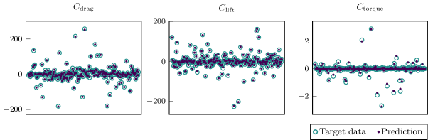
Figure 4: Target data and network prediction for 300 random points in the training data set. Network architecture: 50/20/20, 1653 parameters.

As a result of the above considerations, we choose the single 50/20/20 network for our application of predicting the drag lift and torque from the average velocity around the rigid particle. Considering this network as a function $\mathds{R}^{2}\rightarrow\mathds{R}^{3}$, we can then plot the individual function components as a function of the input in a three dimensional plot. This can be seen in Figure 5. This illustrates that while the drag and lift coefficients are represented by a relatively simple function, the torque coefficient is significantly more involved.

Due to the simple input for the network, requiring two integrals over a relatively small area and a rotation of these two values into the reference configuration, as well as the small size of the network itself, the additional computational effort introduced to the solver by predicting the forces, rather than evaluating them directly, is negligible compared to the effort required to solve the non-linear system resulting from the FEM discretisation of the Navier-Stokes equations.

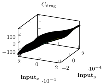
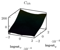
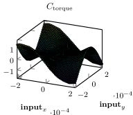
Figure 5: Network prediction components from the 50/20/20 network as functions of input variables.

Remark (Training times).

The training the above networks was performed on a Tesla V100 PCIe 16GB graphics card with PyTorch using CUDA version 10.1. Due to the small size and simple structure of the networks, the training times for 20000 epochs ranged between 277 seconds for the 30/20/10 network and 936 seconds for the 100/50/20/20 network.

3.4 Validation

In the previous section we have compared the network predictions against the “true” values in the sense of the ALE training data. However, the aim for the network is to predict the force values in a CutFEM simulation and to be more accurate than the boundary integral evaluation.

To validate that the neural network predictions are in fact more accurate than the direct evaluation of the forces from the boundary integral, we run a moving domain CutFEM simulation of the set up, with which we generated the training data for $t_{end}=3$. Here we took a background mesh with $h_{max}=10^{-3}$ in the area where we compute the average of the velocity around the triangle and $h_{max}=0.04$ in the remaining part of the domain. The mesh in the averaging area is therefore a factor of 2 smaller than the size of the rigid body. On this mesh we work with unfitted $\texttt{TH}_{2}$ and $\texttt{TH}_{3}$ elements. We then compute the errors of the force prediction and evaluation, by comparing the values against the direct evaluation of a highly resolved ALE computation of the identical set-up. The spatial discretisation is as for the training data generation above. In both cases, the time-step $\Delta t=\nicefrac{{1}}{{300}}$ was chosen.

The resulting prediction errors of the forces in the CutFEM simulation are given in Table 7. Here we find that mean and maximal prediction error are at least one order of magnitude smaller than the direct evaluation. In Figure 6 we plot the resulting forces for a single run of the above computations ($\alpha=0$). This shows, that while there is a visible difference between the prediction and the “ground truth”, the predictions mirror the real forces much better than the direct force computation via the boundary integral evaluation. Here we also note, that there was no significant improvement in the direct evaluation when using higher order elements. We conclude that while the predictions are not perfect, we have significantly improved on the direct computation of the forces on an under resolved computational mesh. However, we also note that we cannot expect any asymptotic mesh convergence here, as the prediction error will begin to dominate once the interface is sufficiently resolved in every time-step.

		$C_{\text{drag}}$		$C_{\text{lift}}$		$C_{\text{torque}}$
Force comp.	Discr.	$\|\cdot\|_{mean}$	$\|\cdot\|_{\infty}$	$\|\cdot\|_{mean}$	$\|\cdot\|_{\infty}$	$\|\cdot\|_{mean}$	$\|\cdot\|_{\infty}$
Evaluation	$\texttt{TH}_{2}$	$7.859\text{\cdot}{10}^{00}$	$8.408\text{\cdot}{10}^{01}$	$1.329\text{\cdot}{10}^{00}$	$3.321\text{\cdot}{10}^{01}$	$1.440\text{\cdot}{10}^{02}$	$2.285\text{\cdot}{10}^{03}$
Prediction	$\texttt{TH}_{2}$	$1.543\text{\cdot}{10}^{00}$	$2.320\text{\cdot}{10}^{01}$	$2.264\text{\cdot}{10}^{-01}$	$4.812\text{\cdot}{10}^{00}$	$1.478\text{\cdot}{10}^{-01}$	$2.917\text{\cdot}{10}^{00}$
Evaluation	$\texttt{TH}_{3}$	$6.589\text{\cdot}{10}^{00}$	$7.172\text{\cdot}{10}^{01}$	$1.471\text{\cdot}{10}^{00}$	$4.147\text{\cdot}{10}^{01}$	$2.411\text{\cdot}{10}^{02}$	$3.919\text{\cdot}{10}^{03}$
Prediction	$\texttt{TH}_{3}$	$1.515\text{\cdot}{10}^{00}$	$2.279\text{\cdot}{10}^{01}$	$2.366\text{\cdot}{10}^{-01}$	$5.050\text{\cdot}{10}^{00}$	$1.479\text{\cdot}{10}^{-01}$	$2.902\text{\cdot}{10}^{00}$

Table 7: Absolute errors in the forces resulting from the direct evaluation of the boundary integrals and the prediction made by the neural network in a CutFEM computation.

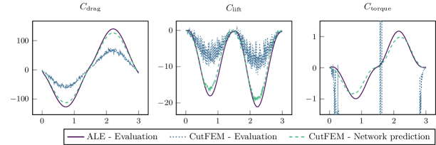
Figure 6: Prediction and evaluation in a CutFEM simulation with $\texttt{TH}_{2}$ elements compared against the values evaluated in a fitted ALE computation.

4 Numerical examples

We consider a number of numerical examples which use the neural network trained in the previous section in an under resolved, moving domain, CutFEM discretisation. The details and analysis of this method as applied to the time-dependent Stokes equations on moving domains is given in [3]. The idea of this method is to use ghost-penalty stabilisation to implement a discrete, implicit extension of the solution into the exterior of the fluid domain, in order to apply a BDF formula to the time derivative in the case of a moving interface. The only modification here is the addition of the convective term. See also [11], where this method has also been applied to a fluid-structure interaction problem with contact and in which the fluid is described by the incompressible Navier-Stokes equations.

To solve the coupled fluid-solid system, we use a partitioned approach. In the sub-step to update the solid velocity we use an update scheme with relaxation, together with Aitken’s $\Delta^{2}$ method [38] to determine the appropriate relaxation parameter and thereby accelerate the relaxation scheme. A relaxation is necessary for stability of the partitioned solver of the coupled system and different relaxation strategies, including Aitken’s $\Delta^{2}$ method are discussed in the literature [39].

Remark 2 (Geometry description in CutFEM).

In CutFEM, numerical integration on elements which are cut by the level-set function describing the geometry, is based on a piecewise linear interpolation of the (smooth) level set function. This is necessary to robustly construct quadrature rules on cut elements, see [4, Section 5.1]. To represent the three sides of the triangular rigid bodies, we therefore use three separate level set functions $\phi_{1}$, $\phi_{2}$ and $\phi_{3}$. ngsxfem [33] then provides the functionality to integrate with respect to each of these level sets, for example the domain where all level sets are negative. Since the level sets describing the sides are linear. the numerical integration on the geometry posed here is exact and we do not have to construct a single level set function $\phi=\max(\phi_{1},\phi_{2},\phi_{3})$ which would then be interpolated into the $\mathbb{P}^{1}$ space on the mesh, which in turn would remove the sharp corners of the particles.

4.1 Example 1: Free-fall restricted to vertical motion

In subsection 3.4 we validated the neural network approach in the setting of prescribed solid motion. To validate the method in our target setting of free-fall, we shall consider the settling of a single particle, restricted to vertical motion as in subsubsection 3.2.1. We consider this simplification, in order to compare the results against a resolved ALE simulation.

To this end we take the domain $\Omega=(0,0.1)^{2}$, assert no-slip boundary conditions at the left and right wall and the do-nothing condition $\mu{F}\nabla\bm{u}\bm{n}=p\bm{n}$ at the top and bottom, see also [40] for details thereon. The rigid body is an equilateral triangle with side-length $2\cdot 10^{-3}$. The fluid and solid material parameters are as in Table 3. At $t=0$ the centre of mass of the rigid body is at $(0.05,0.08)$ and we rotate the body by an angle $\alpha$ with respect to reference configuration, in which the bottom of the triangle is parallel to the $x$-axis. We shall consider $\alpha=0,\pi/12,\pi/6$. See also the left sketch in Figure 7 for an illustration of this initial configuration.

Figure 7: Domain sketches for the initial configurations of the computational examples. Left: A single particle (subsection 4.1 and subsection 4.2). Right: Five particles (subsection 4.3 3).

For the ALE computation we consider $\texttt{TH}_{5}$ elements on a mesh with $h_{max}=$0.005$$, $h=$0.001\,25$$ in a horizontal strip of height $8\text{\cdot}{10}^{-3}$ around the rigid body and $h=$0.0004$$ on the interface of the rigid body. Based on our validation experiments in subsubsection 3.2.2, this discretisation is sufficiently accurate to serve as a reference here.

To ensure that the observed motion is due to our neural network approach, rather than of the discretisation itself, we again consider two different CutFEM simulations. In the first we shall base the solid motion on the forces predicted by the neural network, while in the other the forces are computed by the direct evaluation of the FEM solution. For both CutFEM computations we consider a mesh with $h_{max}=$1\text{\cdot}{10}^{-3}$$ using $\texttt{TH}_{2}$ elements. For the unfitted discretisation used, we take the Nitsche parameter to enforce the Dirichlet boundary conditions on the level set interfaces as $\gamma_{N}=100$ while the stability and extension ghost-penalty parameters are $\gamma_{gp,stab}=0.1$ and $\gamma_{gp,ext}=0.001$ respectively. For details on these parameters we refer to [3].

We take the time-step $\Delta t=\nicefrac{{1}}{{250}}$ and compute until $t=1.0$. For the partitioned fluid-solid solver, we take the initial relaxation parameter as $\omega=0.5$, allow a maximum of 10 sub-iterations per time step and a tolerance of $1\%$ in the relative update.

The forces acting from the fluid onto the rigid body are evaluated using the single 50/20/20 network for drag, lift and torque. As discussed above we use an isoparametric approach to accurately integrate the fluid velocity relative to the solid velocity in $\pazocal{O}(\pazocal{B})$.

In Figure 8 we can see the vertical force, the vertical speed and the vertical position of the centre of mass of the rigid body over time for each of the three triangle orientations. Here we see that for all three orientations, the drag obtained by the network prediction is significantly more accurate than the direct evaluation of the boundary integral. Looking at the body’s vertical speed and position, we see that there is a visible difference between the ALE reference solution and the movement resulting from the predicted forces. The uniformly faster speed in the CutFEM prediction computations can be attributed to the fact, that at small speeds of the particle, the network underestimated the drag, as can be seen in the left column of Figure 8. However we also seen that the predictions are significantly better than the result from the direct evaluation of the forces. This clearly shows, that the neural network approach is able to realise accurate results on very coarse and under resolved meshes, where the unfitted approach with the standard evaluation of the resulting forces does not lead to realistic motion.

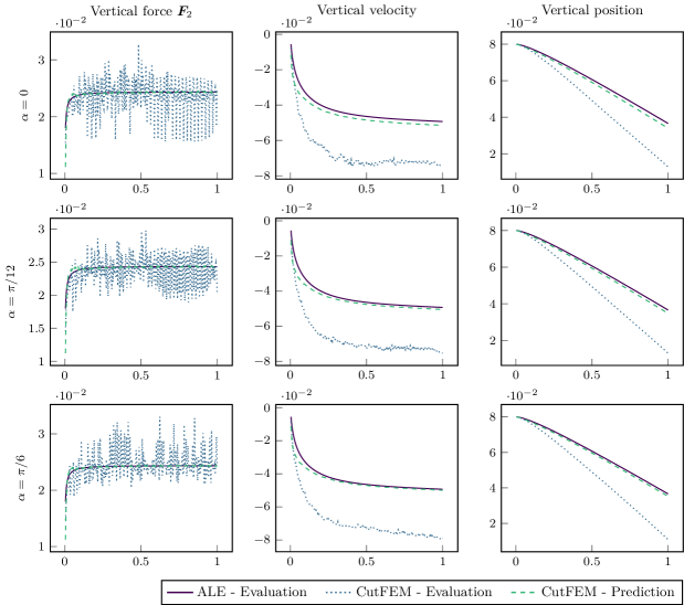
Figure 8: Vertical force, velocity and position of a single falling triangular rigid body restricted to vertical motion. Comparison between an ALE reference computation, the force computation in an under resolved CutFEM computation (Evaluation) and the network prediction (Prediction) in an under resolved CutFEM computation.

4.2 Example 2: Single triangular rigid body

We now consider the full fluid-rigid body system including translational movement in all directions as well as rotational motion. As a result, we do not have an ALE reference to compare the results with. The initial configuration is therefore chosen as in subsection 4.1, with the initial rotation $\alpha=\pi/3$.

We again take the background mesh with $h_{max}=$1\text{\cdot}{10}^{-3}$$ and second mesh with $h_{max}=7.5\cdot 10^{-4}$ to investigate the mesh dependence. On each mesh we take $\texttt{TH}_{2}$ elements. The remaining discretisation parameters are chosen as in the unfitted simulation in subsection 4.1.

In Figure 9 we see the resulting velocity components which make up the movement of the rigid body for the two meshes considered. The fluid solution at time $t=1.0$ on the coarser of the two meshes is visualised in Figure 10.

Looking at velocity components in Figure 9, we immediately see that the influence of the mesh (in the considered under resolved range) is very small. While this does not indicate accuracy of the method, this does show that the method is stable. As is to be expected, the vertical velocity component dominates the translational motion. Furthermore, we see that while a terminal velocity is not fully reached, that the the acceleration between $t=0.5$ and $t=1.5$ is small and the velocity during this time is very similar and only about 10% faster compared to the a priori computations is subsubsection 3.2.1 and in our validation example with restricted motion in subsection 4.1.

The angular velocity in Figure 9 appears very large at first sight. Factoring in that the side-length of the body is $2\cdot 10^{-3}$, we find that the resulting maximal velocity at the corners of the triangular rigid bodies is of order $10^{-2}$. So in general, the velocity of the triangle resulting from rotation is smaller than the vertical velocity component.

Overall, this example shows that our method leads to plausible results on highly under resolved meshes, on which the standard CutFEM approach cannot realise accurate forces and thereby cannot realise accurate solid motion. Finally, we emphasise that a comparison to a fitted ALE simulation is out of scope for this example, since this would have to include re-meshing procedures and projections of the solution onto the resulting new meshes, in order to avoid mesh-entanglement resulting from the rotation of the particles.

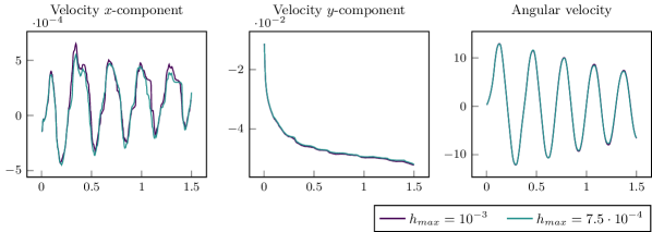
Figure 9: Translational and rotational velocity components of a single triangular rigid body in free fall on an under-resolved mesh with the forces from the predictions by a deep neural network.

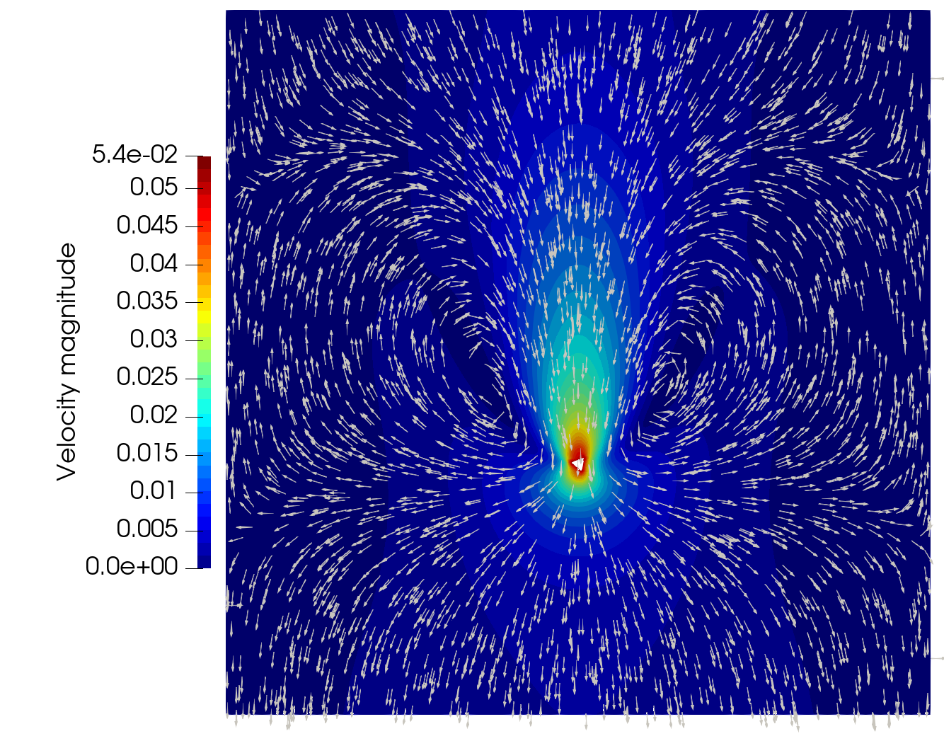
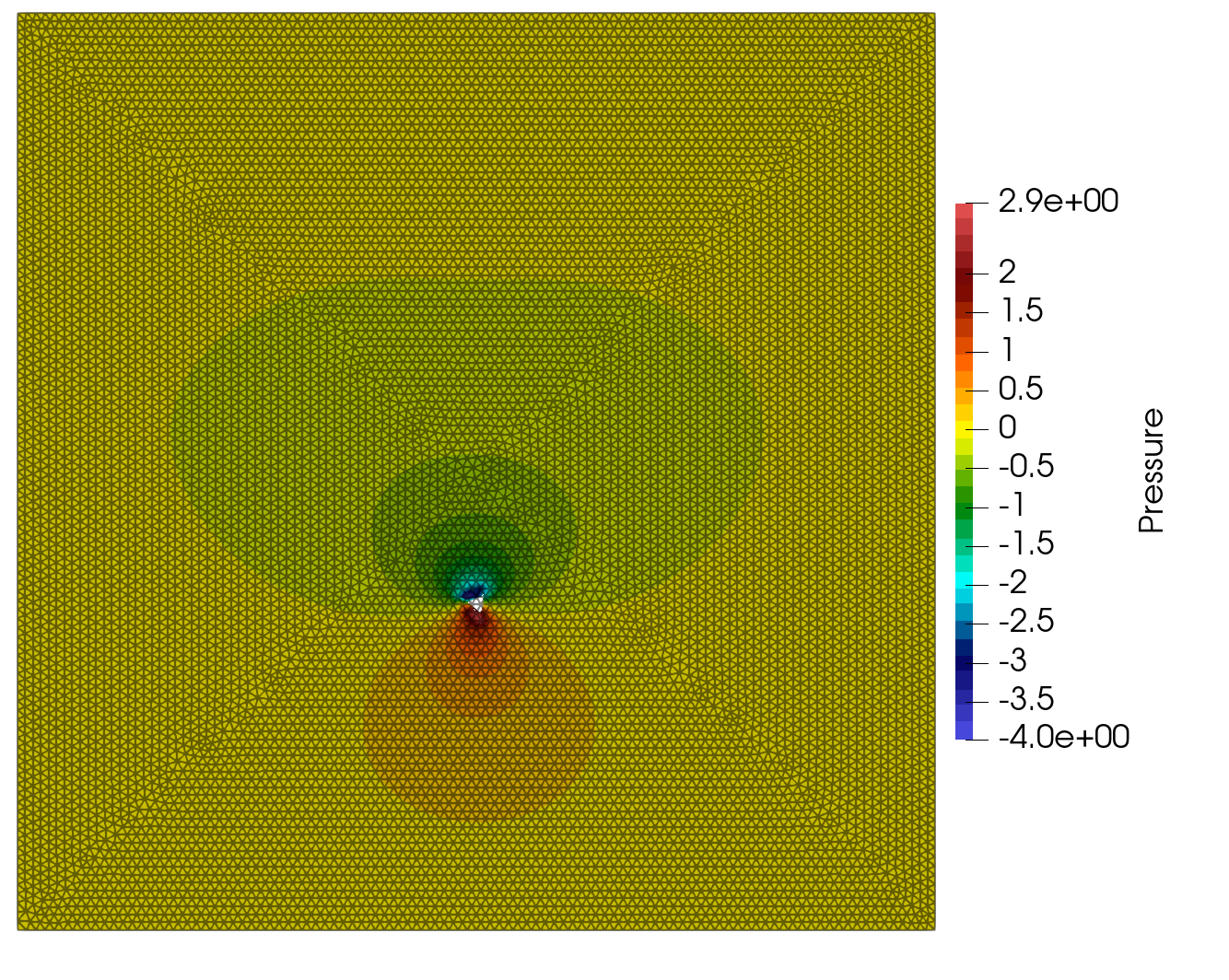
Figure 10: Velocity field (left) and pressure with mesh (right) at $t=1.0$ resulting from a single triangular rigid body in free fall on a mesh with $h_{max}=10^{-3}$ with the forces governing the solid motion obtained from a neural network.

4.3 Example 3: Multiple rigid bodies

As a final more advanced example, consider the same basic set-up as in subsection 4.2, and take 5 rigid triangular rigid bodies denoted by $\pazocal{B}_{i}$, $i=0,\dots,4$.The particles initial position and orientation are then described by their centre of mass as the angle of rotation with respect to the reference configuration, in which the bottom side of the triangle is parallel to the $x$-axis. We denote the initial centre of mass and rotation by $(c_{x},c_{y},\alpha)$. We consider the initial states $(0.035,0.09,0)$, $(0.02,0.065,\pi/6)$, $(0.05,0.06,\pi)$, $(0.075,0.07,\pi/7)$ and $(0.08,0.0925,\pi/13)$ for $\pazocal{B}_{0},\dots,\pazocal{B}_{4}$ respectively. A sketch of this configuration can be seen in the right of Figure 7. The discretisation parameters of the moving domain CutFEM method are all as in subsection 4.2.

The results from these computations are shown in Figure 11 and Figure 12. The translational and rotational velocity components are shown in Figure 11 while the fluid solution at $t=1.0$ is shown in Figure 12.

In Figure 11 we see that there is again no large dependence on the mesh and that in general the translational velocity of all particles are larger than in the single particle case above. Nevertheless, the order of magnitude is the same as before. The slightly faster translational speeds of the particles make sense, as each particle sets the fluid in motion which then helps to transport the other particles. Furthermore we see both in Figure 11 and Figure 12, that $\pazocal{B}_{4}$ has the largest (vertical) velocity. This observation is also meaningful, as $\pazocal{B}_{4}$ is directly in the wake of $\pazocal{B}_{3}$. Furthermore, we note that the angular velocity of $\pazocal{B}_{0}$ and $\pazocal{B}_{4}$, which are above the other particles, is smaller than that of the other particles. We attribute this to the fact, that these two particles are in the parallel flow wake of the other three particles, resulting in a smaller torque acting on these two particles.

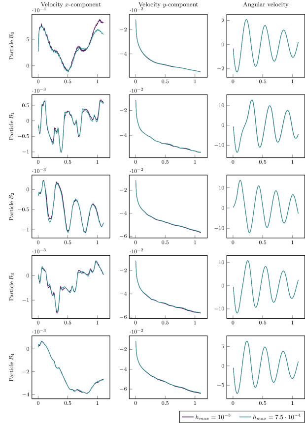
Figure 11: Translational and rotational velocity of five triangular rigid bodies in free fall in an under-resolved CutFEM simulation where the forces governing the solid motion are from the evaluation of a deep neural network.

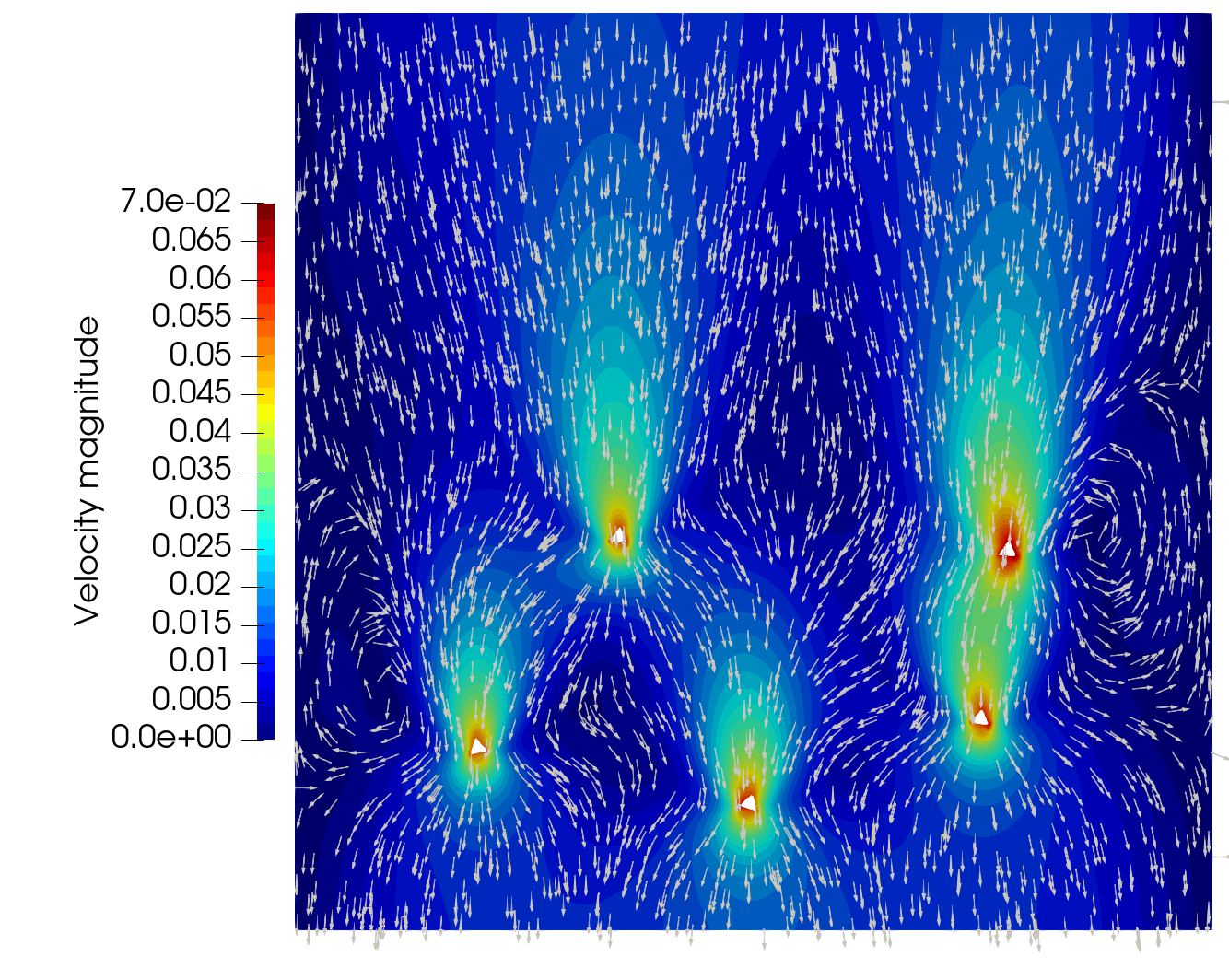
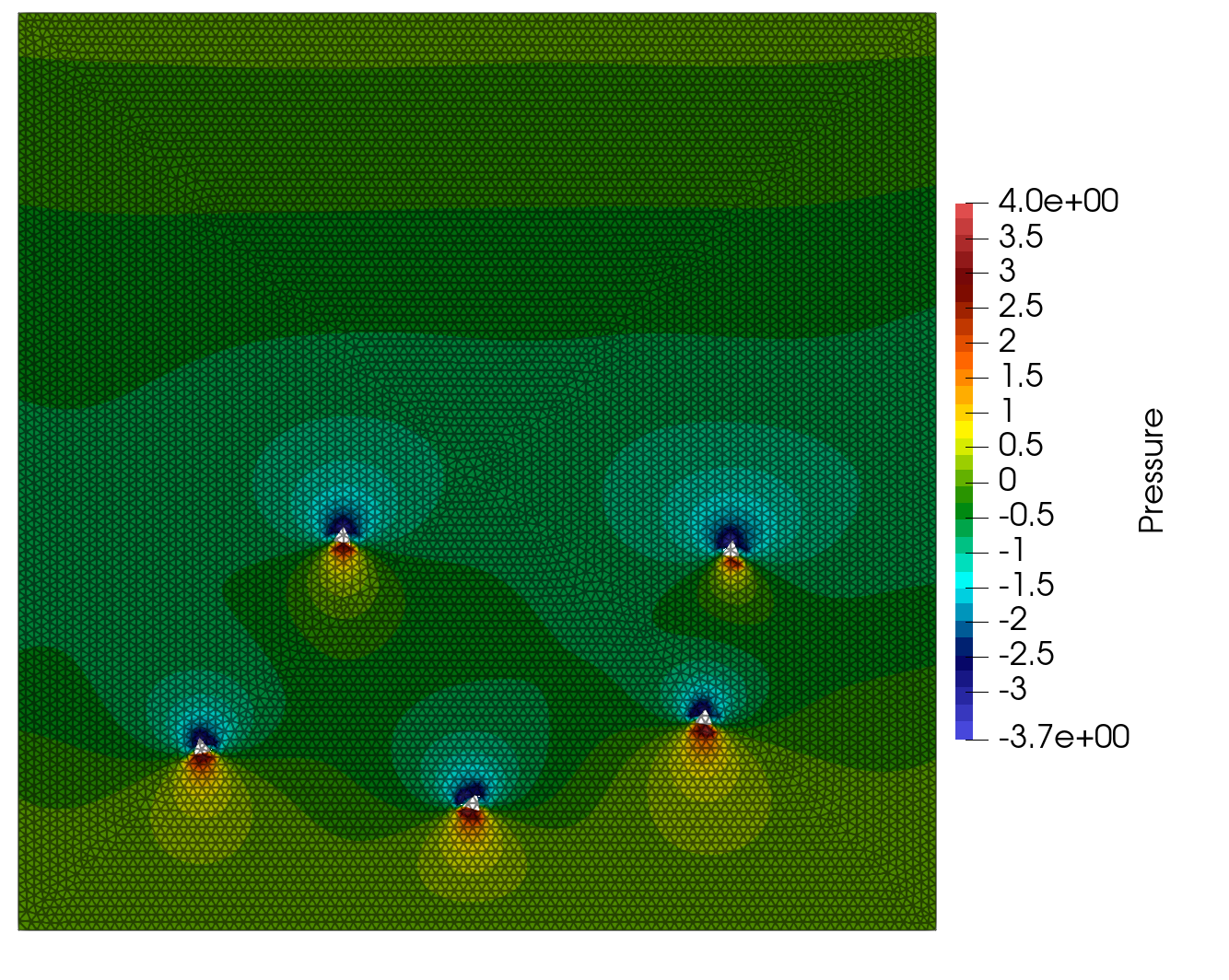
Figure 12: Velocity field (left) and pressure with mesh (right) at $t=1.0$ resulting from five triangular rigid bodies in free fall on a mesh with $h_{max}=10^{-3}$ with the forces governing the solid motion obtained from a neural network.

5 Conclusions and Outlook

Conclusions

We have presented a framework using a hybrid finite element / neural network approach to obtain improved drag lift and torque values acting on a triangular rigid body. For this, we trained a small deep neural network using training data obtained from prototypical motion configurations in resolved finite element simulations. We considered a range of networks by varying the number of layers as well as the number of neurones per layer. Here we saw that the mapping from the average velocity around the particle to the forces acing on this particle was accurately captured by relatively small networks. Applying one of these networks in an under resolved moving domain CutFEM simulation, we showed that this approach results in significantly more accurate force values compared with the direct evaluation of the forces from the finite element solution. We saw that the predicted values were on average an order of magnitude more accurate than the direct evaluation of the forces from the Navier-Stokes solution.

Outlook

A number of interesting questions remain for future research. For example, it would be very interesting to compare the particle motion realised in subsection 4.2 and subsection 4.3 to fitted ALE simulations using re-meshing techniques.

Furthermore, it remains to generalise this approach to other particle shapes and sizes. Here it would also be interesting to see, if a different choice of input data could generalise the approach to use a single neural network to predict accurate forces with different material parameters.

Finally, the method should be extended to the interaction of several closely neighbouring particles as well as to the particle-wall interaction. In particular, extended training data sets have to be created for this purpose. Also, it has to be explored whether it is sufficient to consider the mean ambient velocity as network input in this case or whether further information, e.g. the velocity gradient or acceleration rates of the particles or the fluid should be taken into account.

References

- [1] C. Lehrenfeld and M.. Olshanskii “An Eulerian finite element method for PDEs in time-dependent domains” In ESAIM Math. Model. Numer. Anal. 53.2 EDP Sciences, 2019, pp. 585–614 DOI: 10.1051/m2an/2018068
- [2] E. Burman, S. Frei and A. Massing “Eulerian time-stepping schemes for the non-stationary Stokes equations on time-dependent domains”, 2019 arXiv:1910.03054 [math.NA]
- [3] H. Wahl, T. Richter and C. Lehrenfeld “An unfitted Eulerian finite element method for the time-dependent Stokes problem on moving domains” Accepted In IMA J. Numer. Anal., 2021 DOI: 10.1093/imanum/drab044
- [4] E. Burman, S. Claus, P. Hansbo, M.. Larson and A. Massing “CutFEM: Discretizing geometry and partial differential equations” In Internat. J. Numer. Methods Engrg. 104.7 Wiley, 2014, pp. 472–501 DOI: 10.1002/nme.4823
- [5] R. Felice “The voidage function for fluid-particle interaction systems” In Int. J. Multiph. Flow 20, 1994, pp. 153–159 DOI: 10.1016/0301-9322(94)90011-6
- [6] A. Hölzer and M. Sommerfeld “New simple correlation formula for the drag coefficient of non-spherical particles” In Powder Technol. 184.3 Elsevier BV, 2008, pp. 361–365 DOI: 10.1016/j.powtec.2007.08.021
- [7] M. Mandø and L. Rosendahl “On the motion of non-spherical particles at high Reynolds number” In Powder Technol. 202.1-3 Elsevier BV, 2010, pp. 1–13 DOI: 10.1016/j.powtec.2010.05.001
- [8] M. Zastawny, G. Mallouppas, F. Zhao and B. Wachem “Derivation of drag and lift force and torque coefficients for non-spherical particles in flows” In Int. J. Multiph. Flow 39 Elsevier BV, 2012, pp. 227–239 DOI: 10.1016/j.ijmultiphaseflow.2011.09.004
- [9] W. Zhong, A. Yu, X. Liu, Z. Tong and H. Zhang “DEM/CFD-DEM Modelling of non-spherical particulate systems: Theoretical Developments and Applications” In Powder Technol. 302 Elsevier BV, 2016, pp. 108–152 DOI: 10.1016/j.powtec.2016.07.010
- [10] D. Wan and S. Turek “Fictitious boundary and moving mesh methods for the numerical simulation of rigid particulate flows” In J. Comput. Phys. 222.1 Elsevier BV, 2007, pp. 28–56 DOI: 10.1016/j.jcp.2006.06.002
- [11] H. Wahl, T. Richter, S. Frei and T. Hagemeier “Falling balls in a viscous fluid with contact: Comparing numerical simulations with experimental data” In Phys. Fluids 33.2, 2021 DOI: 10.1063/5.0037971
- [12] T… Hughes, W.. Liu and T.. Zimmermann “Lagrangian-Eulerian finite element formulations for incompressible viscous flows” In Comput. Methods Appl. Mech. Engrg. 29, 1981, pp. 329–349 DOI: 10.1016/0045-7825(81)90049-9
- [13] J. Donea “An arbitrary Lagrangian-Eulerian finite element method for transient dynamic fluid-structure interactions” In Comput. Methods Appl. Mech. Engrg. 33, 1982, pp. 689–723 DOI: 10.1016/0045-7825(82)90128-1
- [14] T. Richter and T. Wick “Finite Elements for Fluid-Structure Interaction in ALE and Fully Eulerian coordinates” In Comput. Methods Appl. Mech. Engrg. 199.41-44, 2010, pp. 2633–2642 DOI: 10.1016/j.cma.2010.04.016
- [15] C.. Peskin “The immersed boundary method” In Acta Numer. 11 Cambridge University Press (CUP), 2002, pp. 479–517 DOI: 10.1017/s0962492902000077
- [16] M. A. Azis, F. Evrard and B. Wachem “An immersed boundary method for flows with dense particle suspensions” In Acta Mech. 230.2 Springer ScienceBusiness Media LLC, 2018, pp. 485–515 DOI: 10.1007/s00707-018-2296-y
- [17] J. Happel and H. Brenner “Low Reynolds number hydrodynamics” Springer Netherlands, 1981 DOI: 10.1007/978-94-009-8352-6
- [18] M. Minakowska, T. Richter and S. Sager “A finite element / neural network framework for modeling suspensions of non-spherical particles.” In Vietnam J. Math. 49.1, 2021, pp. 207–235 DOI: 10.1007/s10013-021-00477-9
- [19] A. Hansbo and P. Hansbo “An unfitted finite element method, based on Nitsche’s method, for elliptic interface problems” In Comput. Methods Appl. Mech. Engrg. 191.47-48, 2002, pp. 5537–5552 DOI: 10.1016/s0045-7825(02)00524-8
- [20] K. Fidkowski and D. Darmofal “A triangular cut-cell adaptive method for high-order discretizations of the compressible Navier–Stokes equations” In J. Comput. Phys. 225.2 Elsevier BV, 2007, pp. 1653–1672 DOI: 10.1016/j.jcp.2007.02.007
- [21] P. Bastian and C. Engwer “An unfitted finite element method using discontinuous Galerkin” In Internat. J. Numer. Methods Engrg. 79.12, 2009, pp. 1557–1576 DOI: 10.1002/nme.2631
- [22] U. Langer and H. Yang “Numerical simulation of parabolic moving and growing interface problems using small mesh deformation”, 2015 arXiv:1507.08784 [math.NA]
- [23] X. Fang “An Isoparametric Finite Element Method for Elliptic Interface Problems with Nonhomogeneous Jump Conditions” In WSEAS Trans. Math. 12, 2013 URL: http://www.wseas.org/multimedia/journals/mathematics/2013/56-222.pdf
- [24] S. Frei and T. Richter “A locally modified parametric finite element method for interface problems” In SIAM J. Num. Anal. 52, 2014, pp. 2315–2334 DOI: 10.1137/130919489
- [25] M. Schäfer and S. Turek “Benchmark computations of laminar flow around a cylinder” In Notes on Numerical Fluid Mechanics (NNFM) Vieweg+Teubner Verlag, 1996, pp. 547–566 DOI: 10.1007/978-3-322-89849-4_39
- [26] I. Babuška and A. Miller “The post-processing approach in the finite element method-part 1: Calculation of displacements, stresses and other higher derivatives of the displacements” In Internat. J. Numer. Methods Engrg. 20.6 Wiley, 1984, pp. 1085–1109 DOI: 10.1002/nme.1620200610
- [27] E. Burman and P. Hansbo “Fictitious domain methods using cut elements: III. A stabilized Nitsche method for Stokes’ problem” In ESAIM Math. Model. Numer. Anal. 48.3 EDP Sciences, 2014, pp. 859–874 DOI: 10.1051/m2an/2013123
- [28] A. Massing, M.. Larson, A. Logg and M.. Rognes “A stabilized Nitsche fictitious domain method for the Stokes problem” In J. Sci. Comput. 61.3 Springer Nature, 2014, pp. 604–628 DOI: 10.1007/s10915-014-9838-9
- [29] C. Lehrenfeld “High order unfitted finite element methods on level set domains using isoparametric mappings” In Comput. Methods Appl. Mech. Engrg. 300 Elsevier BV, 2016, pp. 716–733 DOI: 10.1016/j.cma.2015.12.005
- [30] C. Lehrenfeld “A higher order isoparametric fictitious domain method for level set domains” In Lecture Notes in Computational Science and Engineering 121 Springer, Cham, 2017, pp. 65–92 DOI: 10.1007/978-3-319-71431-8_3
- [31] J. Schöberl “C++11 implementation of finite elements in NGSolve”, 2014 URL: http://www.asc.tuwien.ac.at/~schoeberl/wiki/publications/ngs-cpp11.pdf
- [32] J. Schöberl “NETGEN an advancing front 2D/3D-mesh generator based on abstract rules” In Comput. Vis. Sci. 1.1 Springer Nature, 1997, pp. 41–52 DOI: 10.1007/s007910050004
- [33] C. Lehrenfeld, F. Heimann, J. Preuß and H. Wahl “ngsxfem: An add-on to NGSolve for unfitted finite element discretizations” In J. Open Source Softw., 2021 DOI: 10.21105/joss.03237
- [34] V. John, A. Linke, C. Merdon, M. Neilan and L.. Rebholz “On the divergence constraint in mixed finite element methods for incompressible flows” In SIAM Rev. 59.3 Society for Industrial & Applied Mathematics (SIAM), 2017, pp. 492–544 DOI: 10.1137/15m1047696
- [35] M. Raissi, A. Yazdani and G.. Karniadakis “Hidden fluid mechanics: Learning velocity and pressure fields from flow visualizations” In Science 367.6481 American Association for the Advancement of Science (AAAS), 2020, pp. 1026–1030 DOI: 10.1126/science.aaw4741
- [36] M. Raissi, P. Perdikaris and G.. Karniadakis “Physics-informed neural networks: A deep learning framework for solving forward and inverse problems involving nonlinear partial differential equations” In J. Comput. Phys. 378 Elsevier BV, 2019, pp. 686–707 DOI: 10.1016/j.jcp.2018.10.045
- [37] A. Paszke et al. “PyTorch: An Imperative Style, High-Performance Deep Learning Library” In Advances in Neural Information Processing Systems 32 2 Curran Associates, Inc., 2019, pp. 8026–8037 URL: http://papers.nips.cc/paper/9015-pytorch-an-imperative-style-high-performance-deep-learning-library.pdf
- [38] B.. Irons and R.. Tuck “A version of the Aitken accelerator for computer iteration” In Internat. J. Numer. Methods Engrg. 1.3 Wiley, 1969, pp. 275–277 DOI: 10.1002/nme.1620010306
- [39] U. Küttler and W.. Wall “Fixed-point fluid-structure interaction solvers with dynamic relaxation” In Comput. Mech. 43.1 Springer ScienceBusiness Media LLC, 2008, pp. 61–72 DOI: 10.1007/s00466-008-0255-5
- [40] J.. Heywood, R. Rannacher and S. Turek “Artificial boundaries and flux and pressure conditions for the incompressible Navier-Stokes equations” In Internat. J. Numer. Methods Fluids 22, 1996, pp. 325–352 DOI: 10.1002/(SICI)1097-0363(19960315)22:5<325::AID-FLD307>3.0.CO;2-Y