A spectrally stratified hot accretion flow in the hard state of MAXI J1820+070

Abstract

We study the structure of the accretion flow in the hard state of the black-hole X-ray binary MAXI J1820+070 with NICER data. The power spectra show broadband variability which can be fit with four Lorentzian components peaking at different time scales. Extracting power spectra as a function of energy enables the energy spectra of these different power spectral components to be reconstructed. We found significant spectral differences among Lorentzians, with the one corresponding to the shortest variability time scales displaying the hardest spectrum. Both the variability spectra and the time-averaged spectrum are well-modelled by a disc blackbody and thermal Comptonization, but the presence of (at least) two Comptonization zones with different temperatures and optical depths is required. The disc blackbody component is highly variable, but only in the variability components peaking at the longest time scales ($\lower 2.15277pt\hbox{$\;\buildrel>\over{\sim}\;$}1$ s). The seed photons for the spectrally harder zone come predominantly from the softer Comptonization zone. Our results require the accretion flow in this source to be structured, and cannot be described by a single Comptonization region upscattering disc blackbody photons, and reflection from the disc.

1 Introduction

The majority of known black-hole (BH) X-ray binaries (XRBs) are transient (Coriat et al., 2012). They spend most of their time in a quiescent state, characterized by low/undetectable levels of the X-ray luminosity, $L_{\rm X}/L_{\rm Edd}\lesssim 10^{-5}$ (where $L_{\rm Edd}$ is the Eddington luminosity). After some years of quiescence, they go through X-ray brightening episodes, or outbursts, lasting from a few to tens of months. During an outburst the X-ray spectral and timing properties change dramatically (e.g. Belloni et al., 2005; Homan & Belloni, 2005; Dunn et al., 2010; Muñoz-Darias et al., 2011; Heil et al., 2015), and the source goes through a sequence of different accretion states. At the beginning and at the end of an outburst the source is observed in a hard state, spectrally dominated by a hard X-ray thermal Comptonization component (e.g. a review by Done et al., 2007). During the hard state the source becomes increasingly brighter at almost constant spectral hardness, typically over periods of weeks to a few months. Apart from the dominant hard X-ray Comptonization component, broad band X-ray data show spectral complexity, requiring additional components. Many hard state spectra show a soft component, which can be ascribed, at least partly, to the hardest part of the disc thermal emission (due to intrinsic dissipation and/or hard X-ray irradiation, e.g. Zdziarski & De Marco, 2020), with a typical inner temperature of $kT_{\rm in}\sim 0.1$–0.3 keV. At higher energies, signatures of disc reflection are clearly observed. Fits with relativistic models have yielded controversial results (see Bambi et al. 2021 for a review). Some of these studies support the presence of a disc reaching the immediate vicinity of the innermost stable circular orbit (ISCO) already at relatively low luminosities in the hard state (e.g Miller et al., 2006, 2008; Reis et al., 2008; Reis et al., 2010; Tomsick et al., 2008; Petrucci et al., 2014; García et al., 2015; Wang-Ji et al., 2018). Other studies are instead in agreement with a disc truncated at large radii (a few tens of $R_{\rm g}$, where $R_{\rm g}=GM/c^{2}$ is the gravitational radius and $M$ is the BH mass) from low to high hard-state luminosities (e.g. McClintock et al., 2001; Esin et al., 2001; Done & Diaz Trigo, 2010; Kolehmainen et al., 2014; Plant et al., 2015; Basak & Zdziarski, 2016; Dziełak et al., 2019). The latter results are in line with theoretical models which predict evaporation of the inner disc (Meyer et al., 2000; Petrucci et al., 2008; Begelman & Armitage, 2014; Kylafis & Belloni, 2015; Cao, 2016).

One way to understand the origin of these discrepancies is to consider more complexity in the underlying Comptonization continuum. The continuum is usually assumed to result from scattering of disc photons in an homogeneous region near the BH, which in most cases results in a flat or convex spectral shape. On the other hand, inhomogeneity of the Comptonization region is able to produce additional curvature, resulting in a concave underlying continuum, as often required by the data (Di Salvo et al., 2001; Frontera et al., 2001; Ibragimov et al., 2005; Makishima et al., 2008; Nowak et al., 2011; Yamada et al., 2013; Basak et al., 2017; Zdziarski et al., 2021a). Such conditions can account for both a part of the Fe K line red wing and a part of the reflection hump at $\gtrsim$10 keV, which allow the need for extreme relativistic reflection parameters, as well as a super-solar Fe abundance (often found in the fits, Fürst et al., 2015; García et al., 2015; Parker et al., 2015, 2016; Walton et al., 2016, 2017; Tomsick et al., 2018) to be relaxed. The presence of a radially stratified and spectrally inhomogeneous Comptonization region is independently supported by X-ray variability studies. In particular, the common detection of frequency-dependent hard X-ray lags (hard X-ray variations lagging soft X-ray variations) in energy bands dominated by the primary hard X-ray continuum can be explained by mass accretion rate fluctuations propagating inward (Lyubarskii, 1997; Arévalo & Uttley, 2006). However, in order to detect a net hard lag, the zone these perturbations propagate through must have a radially-dependent emissivity profile, with the inner regions emitting a harder spectrum (Kotov et al., 2001). Spectral-timing techniques, which allow resolving the spectral components contributing to variability on different timescales (frequency-resolved spectroscopy) have been applied to BH XRBs, showing that those spectra generally harden with decreasing time scale. This also provides evidence for the differences in the observed spectral shape to be related to their different distances from the BH, see, e.g. Revnivtsev et al. (1999); Axelsson & Done (2018). Following these findings, Mahmoud & Done (2018) and Mahmoud et al. (2019) created theoretical models reproducing those observations by multi-zone models coupled with propagation mass accretion rate fluctuations.

We study the BH XRB system MAXI J1820+070, focusing on two Neutron star Interior Composition ExploreR (NICER; Gendreau et al. 2016) observations taken during the rise of its 2018 outburst (see De Marco et al., 2021, for a systematic analysis of all the first part of the outburst). We perform frequency-resolved spectroscopy method in the formulation outlined by Axelsson & Done (2018). We fit frequency-resolved energy spectra using Comptonization models, with the goal to constrain the structure of the hot flow, and verify the possible presence of multiple Comptonization zones.

MAXI J1820+070 was first detected in the optical wavelengths by the All-Sky Automated Search for SuperNovae on 2018-03-06 (ASASSN-18ey, Tucker et al., 2018). It was detected in X-rays five days later by the Monitor of All-sky X-ray Image (MAXI; Matsuoka et al. 2009) on board of International Space Station (Kawamuro et al., 2018). The two detections were connected to the same source by Denisenko (2018). It was then identified as a BH candidate (Kawamuro et al., 2018; Shidatsu et al., 2019). Torres et al. (2019) confirmed the presence of a BH by dynamical studies of the system in the optical band, and Torres et al. (2020) measured in detail the parameters of the system. The donor is a low-mass K star and the orbital period is $0.68549\pm 0.00001$ d (Torres et al., 2019).

The BH mass is $M\approx(5.95\pm 0.22){\rm M}_{\sun}/\sin^{3}i$ (Torres et al., 2020), anticorrelated with the binary inclination, $i$. Those authors estimated the latter as $66\degr<i<81\degr$. On the other hand, Atri et al. (2020) estimated the inclination of the jet as $i\approx 63\pm 3\degr$. Based on their radio parallax, Atri et al. (2020) determined the distance to MAXI J1820+070 as $d\approx 3.0\pm 0.3$ kpc, consistent with the Gaia Data Release 2 parallax, yielding $d\approx 3.5^{+2.2}_{-1.0}$ kpc (Bailer-Jones et al., 2018; Gandhi et al., 2019; Atri et al., 2020). MAXI J1820+070 is a relatively bright source, with the peak 1–100 keV flux estimated by Shidatsu et al. (2019) as $\approx\!1.4\times 10^{-7}$ erg cm^-2 s^-1, which corresponds to the isotropic luminosity of $\approx\!1.5(d/3\,{\rm kpc})^{2}\times 10^{38}$ erg s^-1. Assuming an inclination $i=66\degr$ this corresponds to $\sim$15% $L/L_{\rm{Edd}}$. The value of Galactic hydrogen column density toward the source has been estimated in the range of (0.5–$2)\times 10^{21}$ cm^-2 (Uttley et al., 2018; Kajava et al., 2019; Fabian et al., 2020; Xu et al., 2020).

2 Data reduction

For our analysis, we choose two relatively long observations of MAXI J1820+070 carried out by NICER, see Table 1. Hereafter, we refer to the studied observations using only the last three digits of their identification number (ID), i.e. 103 and 104. They correspond to the initial phases of the 2018 outburst, when the source was in the rising hard state (see Figure 1 in De Marco et al. 2021). We estimate their energy fluxes to be $\approx$6.5 and $\approx 9.5\times 10^{-9}$ erg cm^-2 s^-1, respectively, in the 0.3–10 keV energy band.

The data were reduced using the NICERDAS tools in heasoft v.6.25, starting from the unfiltered, calibrated, all Measurement/Power Unit (MPU) merged files, ufa. We applied the standard screening criteria (e.g. Stevens et al., 2018) through the NIMAKETIME and NICERCLEAN tools. We check for periods of high particle background, i.e., with rate $>$2 count s^-1, by inspecting light curves extracted in the energy range of 13–15 keV, in which the contribution from the source is negligible because of the drop in the effective area (Ludlam et al., 2018).

Of the 56 focal plane modules (FPMs) of the NICER X-ray Timing Instrument (XTI), four (FPMs 11, 20, 22, and 60) are not operational. Additionally, we filter out the FPMs 14 and 34, since they are found to occasionally display increased detector noise. Thus, the number of FPMs used for our analysis is 50. In order to correct for the corresponding reduction of effective area, the reported source fluxes were rescaled by the number of used FPMs.

The shortest good time intervals, with the length $<10$ s, were removed from the analysis, resulting in the net, on-source, exposure times reported in Table 1. Filtered event lists were barycentre-corrected and used to extract the light curves and spectra using XSELECT v.2.4e. We used publicly distributed ancillary response and redistribution matrix files as of 2020-02-12 and 2018-04-04, respectively. Fits were performed using the X-Ray Spectral Fitting Package (Xspec v.12.10.1; Arnaud 1996). Hereafter uncertainties are reported at the 90 per cent confidence level for a single parameter.

Table 1: The log of the NICER observations used for the analysis. Exposures correspond to the effective on-source time after data cleaning.

Obs. ID	Start time	Exposure
	[yyyy-mm-dd hh:mm:ss]	[s]
1200120103	2018-03-13 23:56:12	9474
1200120104	2018-03-15 00:36:04	6231

3 Analysis

3.1 Power spectral density

We first compute and fit the power spectral density (PSD) for each of the observations in two broad energy bands, 0.3–2 keV and 2–10 keV, in order to identify components contributing to the observed variability on different timescales. We extract light curves with a time bin of 0.4 ms in these energy bands. The light curves were split into segments of 200 s length. We calculate the PSD of each segment and average them, in order to obtain more accurate estimates of the PSD of each single observations. The chosen time bin and the segment length allow us to cover the range of frequencies of 0.005–1250 Hz. This range well samples both the broad-band noise intrinsic to the source and the Poisson noise level. The latter was fit at frequencies of $\nu>300$ Hz and subtracted from the PSDs at all frequencies. We adopt a logarithmic rebinning in order to improve the statistics at high frequencies.

We normalize the PSDs using the fractional squared root-mean-square units ((rms/mean rate)²Hz^-1, Belloni & Hasinger, 1990; Miyamoto et al., 1992). The PSDs are shown in Fig. 1. Their complex structure hints at the presence of several variability components. As commonly done in the literature (Belloni et al., 1997; Nowak, 2000), we fit each PSD with a sum of Lorentzian components, for which we use Xspec. A Lorentzian is described by

$$P(\nu)=K\frac{\sigma}{2\pi}\frac{1}{(\nu-\nu_{0})^{2}+(\sigma/2)^{2}},$$ (1)

where $K$ is the normalization, $\sigma$ is the full width at half maximum, and $\nu_{0}$ is the centroid frequency. However, the maximum power (i.e. the peak of $\nu P(\nu)$) is observed at the frequency $\nu_{max}>\nu_{0}$ (Belloni et al., 1997)

$$\nu_{\rm{max}}=\sqrt{\nu_{0}^{2}+\left(\frac{\sigma}{2}\right)^{2}}.$$ (2)

We jointly fit the resulting four PSDs, we tie $\nu_{0}$ and $\sigma$ parameters, but allow for different normalization. We start with fitting a single Lorentzian, and add a new one if significant residuals remained. We find that the hard band is well described by four Lorentzian components, but an addition of the highest-frequency, fourth, Lorentzian in the soft band PSD yields a normalization consistent with zero. We also find that letting $\nu_{0}$ and $\sigma$ vary independently for each PSD does not lead to significant fit improvements. Therefore, our final joint model consists of four Lorentzians (hereafter L1, L2, L3, and L4), with the parameters given in Table 2. The Poisson noise subtracted PSDs with the best-fit models are shown in Fig. 1.

We check that the PSDs of the two observations have compatible shape and consistent fractional normalization in each of the two energy bands ( $\approx$32 and $\approx$27 per cent in the soft and hard band, respectively). This means that there is no significant deviation from stationarity between the two observations. Therefore, we decide to combine the two observations in order to obtain a higher signal-to-noise for the remainder of our analysis.

Table 2: The results of the joint fits of the PSDs of the observations 103 and 104 in the 0.3–2 keV and 2–10 keV energy bands with the model consisting of four Lorentzians, see equation (1). We also give the resulting peak frequency of $\nu P(\nu)$, equation (2), and the resulting reduced $\chi^{2}$.

	L1	L2	L3	L4
$\nu_{\rm{0}}$ [Hz]	0+0.006	0.095${}^{+0.038}_{-0.039}$	1.59${}^{+0.16}_{-0.18}$	0.65${}^{+0.27}_{-0.65}$
$\sigma$ [Hz]	0.045${}^{+0.004}_{-0.003}$	0.96${}^{+0.09}_{-0.08}$	3.07${}^{+0.11}_{-0.09}$	4.80${}^{+1.01}_{-0.35}$
$\nu_{\rm{max}}$ [Hz]	0.023${}^{+0.002}_{-0.002}$	0.489${}^{+0.045}_{-0.039}$	2.21${}^{+0.12}_{-0.13}$	2.49${}^{+0.49}_{-0.24}$
$\chi^{2}_{\nu}$	0.993

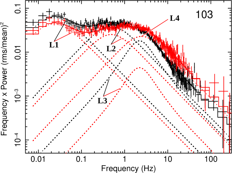
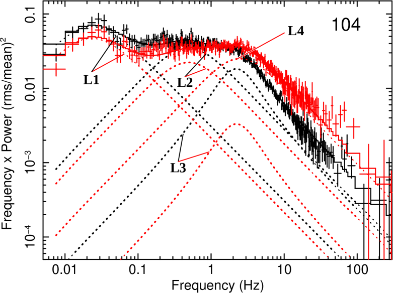
Figure 1: The Poisson noise subtracted PSDs of the two analyzed observations in the two energy bands, 0.3–2 keV (black symbols) and 2–10 keV (red symbols). The total best-fit models (solid lines) and the Lorentzian components of the model (dotted curves) are also shown.

3.2 Extraction of frequency-resolved spectra

We extract the fractional rms and absolute rms energy spectra using the Lorentzian fits presented in Section 3.1. The fractional rms spectrum shows the distribution of fractional variability power as a function of energy (e.g. Vaughan et al., 2003) and can be used to readily assess the presence of spectral variability (e.g. presence of multiple variable spectral components, spectral pivoting). On the other hand, the absolute rms spectrum shows the spectral shape of the components that contribute to variability, and can be used to directly fit spectral models. However, this comes with some caveats that will be discussed in Sect. 4. We use the technique proposed by Axelsson et al. (2013). We create a logarithmic energy grid with 47 bins in the 0.3–9.9 keV energy range. We then calculate the PSD in fractional (rms/mean rate)²Hz^-1 and absolute units ((count s^-1)²Hz^-1, Vaughan et al., 2003) for each of the bins. We then fit the PSD in each band with the same Lorentzian components as the best-fit model to the PSD of the broad energy bands (Table 2), keeping the values of $\nu_{0}$ and $\sigma$ fixed, and allowing only the normalization of each Lorentzian to vary. The best-fit PSD models for each narrow energy band are then used to extract the fractional and absolute rms variability amplitude spectrum of each Lorentzian. To this aim we analytically integrate the best-fit Lorentzians within the frequency range 0.001–1000 Hz, such that:

$$rms=\sqrt{\left(\frac{K}{\pi}\right)\arctan\left(\frac{(\nu-\nu_{0})}{\sigma/2}\right)\bigg{\rvert}_{\nu=0.001}^{\nu=1000}}.$$ (3)

We plot these values as a function of energy to obtain the fractional and absolute rms spectra. Results are reported in Fig. 2. We note that since these four components were obtained from the power spectrum, which gives rms², they were assumed to be completely uncorrelated, and, in order to obtain the total rms spectrum, the single rms spectra have to be summed in quadrature. We note that the rms spectra have the redistribution matrix obtained by rebinning the matrix for the average spectrum.

The errors on the rms spectra were calculated based on the $1\sigma$ deviation of the normalization of the best-fit Lorentzians. To this aim, for each Lorentzian and in each energy band, we draw two random numbers distributed according to a Gaussian distribution with the mean equal to the best-fit value of the normalization, $K$, and the standard deviation equal to its $1\sigma$ lower/upper error of $K$. This procedure was repeated 100 times for each Lorentzian component, resulting in two sets of 100 simulations each. We use each set to estimate the upper and lower limits on the rms in every energy channel. In order to have symmetric errors (as required in Xspec) we take the average of the obtained upper and lower errors. The unconstrained points, i.e., those resulting in upper limits on the rms (e.g. as in the case of the normalization of L4 in the softest energy bands) were omitted in the fits and are not presented in the plots.

The fractional rms spectra of each Lorentzian show significant spectral variability (Fig. 2, left). In particular, in the low frequency components (L1, L2, and L3) a local peak of variability is observed at around 1 keV (at the peak the fractional rms decreases from $\sim$36% to $\sim$18% from low to high frequencies). Then, on either side of the peak the fractional rms tends to decrease. While for L1 and L2 the decrease is steady up to the highest sampled energies, for L3 a reversal of this trend is observed above $\sim$3 keV. L4 does not show any low energy peak, and the variability at around $\sim$1 keV results suppressed. In L1, L2, and L4 the fractional variability appears to flatten out at energies $\gtrsim$3 keV (to a level of $\sim$26% for L1, and $\sim$20% for L2 and L4). This suggests that high energy spectral components predominantly vary in normalization only. We note that these results are in agreement with those reported by Axelsson & Veledina (2021).

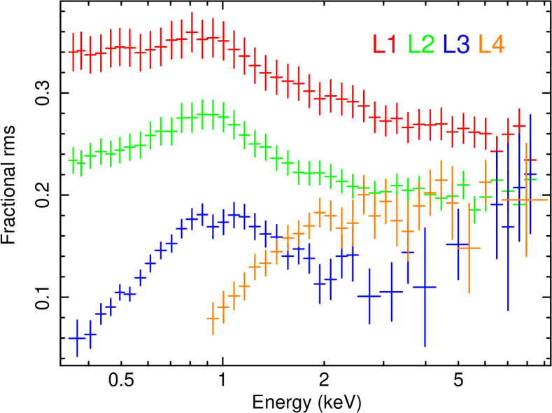
Figure 2: The fractional rms spectra (left panel) and absolute rms spectra (right panel) of each of the four Lorentzian components, unfolded to a constant model.

3.3 Spectral fits of absolute rms and time-averaged spectra

We then proceed to fit absolute rms and time-averaged spectra, using standard Xspec models. In our models, absorption due to the interstellar medium (ISM) is modeled using tbabs (Wilms et al., 2000), with the elemental abundances from the same paper. We model thermal Comptonization using the model ThComp (Zdziarski et al., 2020). Since this is a convolution model, the covered energy range has to be extended beyond that of the NICER spectra in order to get a full range of energies for the seed photons; we use the range of 0.01 keV–2000 keV. Since at high energies the sensitivity of the instrument is limited to $E\lower 2.15277pt\hbox{$\;\buildrel<\over{\sim}\;$}10$ keV, we are not able to fit the electron temperature, and we fix it at $kT_{\rm{e}}=50$ keV, which closely resembles the values found from simultaneous fits of NuSTAR data (Zdziarski et al., 2021b). In our modelization, we assume that all the parameters governing the shape of the spectral components are constant and that the variability associated within each Lorentzian is predominantly due to variations in normalization of the spectral components. In particular, our modelization discards spectral pivoting, as suggested by fractional rms spectra (Fig. 2, left; see also Discussion in Sect. 4).

We first consider single Comptonization models, with the disc thermal emission (Mitsuda et al., 1984) being the source of seed photons. The ISM hydrogen column density is fixed at $N_{\rm H}=1.4\times 10^{21}{\rm cm^{-2}}$ (which is the best-fit value obtained from our fit to the time-averaged spectrum, see Table 4 below). ThComp has the fraction of the seed photons incident on the Comptonization region, $f$, as a free parameter. However, we hereafter set $f=1$ and include a separate disc blackbody component with the same parameters in order to separate the two components in the plots and tables. The Xspec notation of the model is TBabs(diskbb₁+ThComp(diskbb₂)). We note that such additive form of the variability model spectrum assumes that the two spectral components are fully correlated. In our first case, Model A, we fit rms spectra of each Lorentzian (L1, L2, L3, L4) with the same parameters except for the normalizations. The normalization of thComp is given by the normalization of the convolved diskbb model. The other free parameters are the inner disc temperature, $kT_{\rm in}$, and the low-energy spectral index of the Comptonization spectrum, $\Gamma$ (defined by the energy flux, $F(E)\propto E^{1-\Gamma}$). The obtained best-fit parameters are given in Table 3 and the ratios of the data to the model are shown in Fig. 3 (top panel). We find that this model provides a rather poor description of the data, $\chi_{\nu}^{2}\approx 318.8/160$.

We thus check if a more complex spectral structure can improve the fits. In Model B, we allow for the photon index, $\Gamma$, to vary among different Lorentzians. This means that we assume the presence of four different Comptonization zones with different Thomson optical depths, $\tau_{\rm T}$, since the spectral index is a function of both $kT_{\rm e}$ and $\tau_{\rm T}$ (see eq. 14 in Zdziarski et al. 2020; and Sunyaev & Titarchuk 1980 for a general discussion).

In Model C, we also allow for changes among $kT_{\rm{in}}$ of the seeds for Comptonization, and allow them to be different from the directly observed disc blackbody. However, we find the seed photons temperature of the rms spectrum of L1 to be unconstrained, so we keep it equal to $kT_{\rm{in}}$ of the directly observed disc. Model C assumes the presence of four different disc blackbodies. While it is unrealistic, we include it as a phenomenological description in order to highlight that the data do require the seed photons to have different characteristic energies for different components. The best-fit parameters of Models B and C are given in Table 3, while the ratios of the data to the corresponding best-fit models are shown in Fig. 3 (middle and bottom panel).

Comparing results from the spectral fits of Model A with those of B and C, we see significant evidence for changes of the spectral properties between the rms spectra of the different Lorentzians. In particular, the fit improves when letting an increasing number of parameters free to vary among the different variability components (from model A to model C, $\Delta\chi^{2}\approx-133$). The data show that the two lowest frequency Lorentzians L1 and L2 have very similar spectra, L3 has the softest spectrum (we note that in this case, the poor signal-to-noise at high energies may be the reason for such softening), and L4 has the hardest spectrum. We also observe that the rms spectrum of the highest frequency Lorentzian (L4) is best fit by a much higher seed photons temperature ($kT_{\rm{in2}}$ in Table 3) than the lower frequency components. This hints at a different source of seed photons for L4, thus suggesting that the innermost parts of the accretion flow are fueled by photons with higher temperature than those fueling the outer parts.

Given the clear indications of changes in spectral properties among different Lorentzian components, we model now the rms spectra and the time-averaged spectrum simultaneously, with the aim of obtaining more robust and self-consistent constraints on the structure of the Comptonization region. For consistency with the rms spectra, the time-averaged spectra of observations 103 and 104 were averaged (using MATHPHA in ftools). The resulting spectrum was rebinned so as to have a minimum of 3 original energy channels and signal-to-noise $\geq$50 in each new energy channel. To account for uncertainties in the current calibration, a systematic error of 1 per cent was added. (Note that this step is not required for the rms spectra, owing to their lower resolution.) Given the limited bandpass of NICER, we did not include complex reflection models in the fits, which would result in overfitting the rms spectra. Therefore, we model the fluorescent Fe K line with a simple Gaussian component.

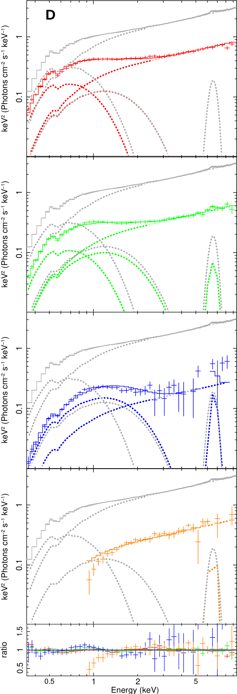
Figure 5: The best-fit models and data of the Lorentzian spectral components (from top to bottom: L1, L2, L3, L4), and the data-to-model ratios (bottom panel) of model D. The colour code is the same as in Fig. 2, and the time-averaged spectrum and its residuals are shown in grey.

Results obtained from our fits with model C show that the overall spectrum cannot be fit by a single Comptonization component. We therefore test for a more complex model, assuming that the hot flow can be described by two Comptonization zones. The model, denoted as D, comprises a directly visible disc (zone I), which photons are upscattered in the outer Comptonization zone II, and those upscattered photons are partly directly observed and partly are upscattered in the inner Comptonization zone III, as illustrated in the drawing in Fig. 4 (top panel). The Xspec notation is given in the caption to Table 4. Again, the underlying assumption is that the three components are fully correlated. The unabsorbed best-fit model to the time-averaged spectrum with these components is presented in Fig. 4 (bottom panel). Since the Fe line is unconstrained in the rms spectra, we require their normalizations to be $\leq$ than that in the time-averaged spectrum. The best-fit parameters are given in Table 4, and the best-fit model and the data-to-model ratios are shown in Fig. 5. We find that model D can simultaneously describe the time-averaged and rms spectra well, with $\chi_{\nu}^{2}\approx 370.4/415$. These results can be summarized as follows.

Low frequency Lorentzians (L1 and L2): In model D, the rms spectra of L1 and L2 show significant contributions from all of their spectral components (see normalizations in Table 4). Still, most of the photons related to the variability component piking at frequencies $\lesssim$1 Hz are associated with the direct disc emission, which variable components comprise $\approx$63 per cent of the total (time-average) disc blackbody flux at the best fit. In zone II, the variable components actually exceed the corresponding time-average, which implies an inaccuracy resulting from the assumed spectral model (see Section 4). Still, it indicates that most of the photons in this zone are variable.

High frequency Lorentzians (L3 and L4): These variability components show no direct emission from the disc at the best fit. This means that the disc gives low contribution to the variability components peaking at the time scales $\gtrsim$1 Hz. Almost all blackbody photons are instead used as seeds for the Comptonization regions. For L3, $\approx$3/4 of those seed photons are Compton upscattered in the outer Comptonization region (zone II), and $\approx$1/4 of them, in the inner Comptonization region (zone III). On the other hand, for L4, most of the disc photons upscattered in the outer Comptonization region (zone II) are used as seed photons for the inner Comptonization region (zone III).

In the model, emission from the inner Comptonization region dominates the bolometric X-ray flux. The outer Comptonization region is significantly softer than the inner one, i.e., $\Gamma_{1}>\Gamma_{2}$. Overall, these results show that the structure for the accretion flow in the hard state is quite complex, with stratified Comptonization regions.

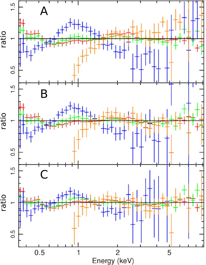
Figure 3: The data-to-model ratios of models A, B, C (from top to bottom; see Table 3). The same colour coding as in Fig. 2 is used: L1 – red, L2 – green, L3 – blue and L4 – orange.

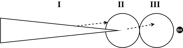
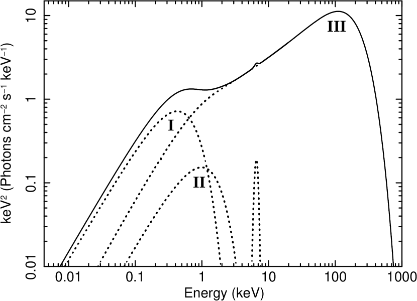
Figure 4: (Top panel): a drawing of the geometry assumed in model D. (Bottom panel) the unabsorbed best-fit to the time-averaged spectrum (solid curve) and its components (dotted curves) marked by the zones shown in the top panel and Table 4.

Table 3: The joint fit results for models with a single Comptonization zone for each of the Lorentzians (L1, L2, L3, L4). The Xspec notation is TBabs(diskbb₁+ThComp(diskbb₂)). The normalization of thComp is given by the normalization of the convolved diskbb model. In model A, the Comptonization plasmas have the same parameters for all of the Lorentzians, and in model B, they can differ in the optical depth, resulting in different spectral indices, $\Gamma$. Model C is a phenomenological one, in which the inner disc temperatures, $kT_{\rm in2}$, of the seed photons for Comptonization can also differ between the Lorentzians. Hereafter, the parameters assumed to be fixed are denoted by (F).

A

B

C

Component

Parameter

L1

L2

L3

L4

L1

L2

L3

L4

L1

L2

L3

L4

TBabs

$N_{\rm{H}}$ [1021 cm-2]

1.4 (F)

1.4 (F)

1.4 (F)

diskbb1

$kT_{\rm{in1}}$ [keV]

0.24${}^{+0.01}_{-0.01}$

0.23${}^{+0.01}_{-0.01}$

0.21${}^{+0.01}_{-0.01}$

$N_{1}$ [103]

15.8${}^{+2.4}_{-1.9}$

8.1${}^{+0.5}_{-0.5}$

3.2${}^{+0.5}_{-0.5}$

0+0.1

19.0${}^{+3.3}_{-2.6}$

13.7${}^{+2.1}_{-1.8}$

0+0.4

0+0.4

23.7${}^{+4.7}_{-3.7}$

19.6${}^{+4.0}_{-3.6}$

0+0.8

0+0.8

ThComp

$\Gamma$

1.56${}^{+0.03}_{-0.03}$

1.64${}^{+0.04}_{-0.04}$

1.63${}^{+0.05}_{-0.05}$

1.91${}^{+0.06}_{-0.05}$

1.32${}^{+0.06}_{-0.06}$

1.67${}^{+0.04}_{-0.04}$

1.64${}^{+0.05}_{-0.05}$

2.20${}^{+0.18}_{-0.13}$

1.48${}^{+0.27}_{-0.13}$

$kT_{\rm{e}}$ [keV]

50 (F)

50 (F)

50 (F)

diskbb2

$kT_{\rm{in2}}$ [keV]

= $kT_{\rm{in1}}$

= $kT_{\rm{in1}}$

= $kT_{\rm{in1}}$

0.34${}^{+0.11}_{-0.09}$

0.32${}^{+0.03}_{-0.03}$

0.83${}^{+0.39}_{-0.29}$

$N_{2}$ [103]

8.1 ${}^{+1.7}_{-1.3}$

6.1${}^{+1.2}_{-0.9}$

4.9${}^{+1.0}_{-0.8}$

5.2${}^{+0.9}_{-0.7}$

12.5${}^{+2.8}_{-2.2}$

8.9${}^{+2.1}_{-1.6}$

9.7${}^{+1.6}_{-1.3}$

5.7${}^{+0.9}_{-0.7}$

16.8${}^{+3.0}_{-3.3}$

2.1${}^{+3.4}_{-1.4}$

2.8${}^{+1.1}_{-0.8}$

0.07${}^{+0.30}_{-0.05}$

$\chi_{\nu}^{2}$

318.8/160

232.7/157

185.9/154

Table 4: The joint fit results for model D with disc blackbody and two Comptonization zones for each of the rms components and the time-averaged spectrum, S_av. The Xspec notation is TBabs(diskbb₁+ThComp₁(diskbb₂)+ThComp₂(ThComp₁(diskbb₃))+Gaussian). The single diskbb emission is split between three parts with the same $kT_{\rm in}$ and different normalizations, $N_{1}$, $N_{2}$ and $N_{3}$. The Roman numbers correspond to the zones shown in Fig. 4. The component fluxes, $F$, are unabsorbed and bolometric (measured in the energy range 0.001-2000keV).

			D
	Component	Parameter	L1	L2	L3	L4	Sav
	TBabs	$N_{\rm{H}}$ [1021 cm-2]	1.4${}^{+0.1}_{-0.1}$
I	diskbb1	$kT_{\rm{in}}$ [keV]	0.18${}^{+0.01}_{-0.01}$
		$N_{1}$ [103]	52.7${}^{+10.2}_{-9.8}$	34.8${}^{+9.8}_{-6.4}$	0+3.2	0+1.4	100.6${}^{+30.1}_{-18.8}$
	$F\,[10^{-9}\,{\rm erg\,cm}^{-2}\,{\rm s}^{-1}$]		1.21${}^{+0.23}_{-0.22}$	0.79${}^{+0.23}_{-0.15}$	0+0.07	0+0.03	2.31${}^{+0.69}_{-0.43}$
II	ThComp1	$\Gamma_{1}$	1.65${}^{+0.14}_{-0.13}$
		$kT_{\rm{e1}}$ [keV]	0.34${}^{+0.04}_{-0.03}$
	diskbb2	$N_{2}$ [103]	8.9${}^{+3.8}_{-2.2}$	7.1${}^{+2.9}_{-1.7}$	10.6${}^{+1.8}_{-1.5}$	0+0.5	8.9${}^{+4.2}_{-2.4}$
	$F\,[10^{-9}\,{\rm erg\,cm}^{-2}\,{\rm s}^{-1}$]		0.47${}^{+0.21}_{-0.11}$	0.38${}^{+0.19}_{-0.11}$	0.57${}^{+0.12}_{-0.09}$	0+0.03	0.48${}^{+0.27}_{-0.16}$
III	ThComp2	$\Gamma_{2}$	1.49${}^{+0.01}_{-0.01}$
		$kT_{\rm{e2}}$ [keV]	50 (F)
	diskbb3	$N_{3}$ [103]	13.5${}^{+2.9}_{-1.8}$	9.9${}^{+2.1}_{-1.3}$	4.7${}^{+1.3}_{-0.8}$	9.3${}^{+1.3}_{-1.1}$	48.6${}^{+9.8}_{-6.1}$
	$F\,[10^{-9}\,{\rm erg\,cm}^{-2}\,{\rm s}^{-1}$]		14.61${}^{+3.16}_{-1.93}$	10.75${}^{+8.48}_{-2.06}$	5.08${}^{+1.28}_{-0.77}$	10.06${}^{+1.23}_{-1.05}$	52.64${}^{+9.56}_{-5.91}$
	Gaussian	$E$ [keV]	6.5${}^{+0.1}_{-0.1}$
		$\sigma$ [keV]	0.39${}^{+0.04}_{-0.08}$
		$N\,[10^{-3}\,{\rm cm}^{-2}\,{\rm s}^{-1}$]	0+1.06	0+4.3	0+4.3	0+4.3	4.3${}^{+0.8}_{-0.8}$
	$\chi_{\nu}^{2}$		157.793/150				213.571/255
			370.4/415

4 Discussion

In our approach, spectral components derived from variability on different time scales are thought to originate from regions of the accretion flow related to these time scales. Generally, we expect the characteristic variability time scale to decrease with the decreasing radial distance from the BH. However, connecting variability time scales to radii is far from simple. Detailed spectro-timing models for Cyg X-1 and GX 339–4, in which such radii were identified, were performed by Mahmoud & Done (2018) and Mahmoud et al. (2019). In particular, the former work found evidence for the existence of discrete regions of enhanced turbulence corresponding to humps in the power spectra.

Here, we simply compare the characteristic Keplerian frequency, $\nu_{\rm K}\equiv(GM)^{1/2}/(2\pi R^{3/2})$ to the characteristic frequencies of our power spectrum, to identify the corresponding characteristic radii. Since this frequency corresponds to the fastest possible variability, it sets an upper limit on the actual emitting radii. This can be written as

$$\frac{R}{R_{\rm g}}\lesssim\frac{c^{2}}{\left(2\pi GM\nu\right)^{2/3}}\approx 250\left(\frac{M}{8{\rm M}_{\sun}}\right)^{-2/3}\left(\frac{\nu}{1\,{\rm Hz}}\right)^{-2/3}.$$ (4)

For the highest peak frequency in the power spectrum, $\approx$2.5 Hz (L4 in Table 2), we have $R/R_{\rm g}\lesssim 140$. We can compare it with the radius based on the disc blackbody normalization, using its definition in Xspec (stress free inner boundary condition is not included as defined in diskbb).We used the total normalization in the time-averaged spectrum in model D, ($N_{1}+N_{2}+N_{3}$). However, this might overestimate the real amount of seed photons from the disc if other sources of seed photons are present (e.g. with little overlap between the disc and the hot flow synchrotron emission might represent this additional source, e.g. Poutanen et al., 2018; Veledina et al., 2011). Therefore, our fits allow us to put an upper limit on $R_{\rm in}$, that corresponds to the real value if the thermal photons from the disc are the only source of seed photons. We find,

$$R_{\rm in} \lesssim 5.3^{+0.5}_{-0.3}\left(\frac{\kappa}{1.7}\right)^{2}\frac{d}{3\,{\rm kpc}}\left(\frac{\cos i}{\cos 65\degr}\right)^{-1/2}10^{7}\,{\rm cm}\approx$$ (5)

$$\approx 45^{+4}_{-3}\left(\frac{M}{8{\rm M}_{\sun}}\right)^{-1}\left(\frac{\kappa}{1.7}\right)^{2}\frac{d}{3\,{\rm kpc}}\left(\frac{\cos i}{\cos 65\degr}\right)^{-1/2}R_{\rm g},$$ (6)

where $\kappa\approx 1.5$–1.9 is the disc blackbody colour correction (e.g. Davis et al. 2005). This satisfies the constraint (4), and shows the disc may be significantly truncated. Then, the hot accretion flow zones II and III can fit downstream of $R_{\rm in}$, showing the self-consistency of this aspect of model D.

Our findings are valid under the assumption that that variability is only due to changes in the normalization of each spectral component. In reality the situation might be much more complex, e.g. as a consequence of spectral pivoting associated with each Comptonization zone. A more rigorous approach implies building appropriate models of the time-variable spectrum, e.g. by perturbing the parameters of the time-averaged spectrum (Gierliński & Zdziarski, 2005) or by solving the Kompaneets equation (Karpouzas et al., 2020; García et al., 2021). Nonetheless, we checked whether spectral pivoting may have a strong influence on our results, by calculating the fractional rms spectra of of each Lorentzian (Fig. 2 - left panel). We observe that the fractional rms generally flattens out at energies $\gtrsim$3 keV. This suggests that high energy spectral components predominantly vary in normalization only, thus supporting our initial assumption. These caveats apply also when modeling disk blackbody emission. Indeed, the changes of the blackbody flux are connected to the changes of its temperature, so assuming only variations of normalization results in overestimating the real temperature in fits of rms spectra (van Paradijs & Lewin, 1986).

The question our research directly addressed was the structure of the accretion flow. Detailed modelling of Comptonization in the accretion flow appears not unique. Clearly, this flow does not consist of a single uniform plasma cloud, as shown by the failure of our model A to describe the rms spectra. Our model B (Table 3) shows that a significant improvement is achieved when allowing the slopes of the rms spectra to differ between the components, in agreement with what is seen in Fig. 2. This can be due to the parameters of the Comptonizing cloud, namely the optical depth and electron temperature, evolving along the accretion flow, and forming distinct zones.

Our model C points to the average energy of the seed photons for Comptonization to vary between the rms spectra of each Lorentzian component. The inner temperature for L1 is weakly constrained, but consistent with being the same as that of the directly observed disc blackbody; those for L2 and L3 are somewhat larger, and the seed photons for L4 have significantly higher temperature, $kT_{\rm in}\approx 0.5$–1.2 keV. This may suggest that photons upscattered in one zone serve as the seed photons for the subsequent zones (as in the models of Axelsson & Done 2018 and Mahmoud & Done 2018). Alternatively, there could be cold clumps formed by some instabilities in the inner parts of the hot flow (e.g. Wu et al. 2016; see Poutanen et al. 2018 for consequences for radiative cooling). Still, even this model leaves significant residuals after the fit, with the actual spectrum of L4 having a sharper low-energy cutoff than that in the fitted model, see Fig. 3. Disc blackbody emission is significant in the rms spectra of the two lower frequency Lorentzians (L1 and L2), meaning that the disc strongly varies on long time scales ($\nu_{max}\lesssim$1 Hz, Table 3 model B and C). On the other hand, the direct disc blackbody emission is not observed in the rms spectra of L3 and L4, meaning that the disc does not contribute significantly to the high frequency variability components ($\nu_{max}>$1Hz). At the same time, Comptonization emission varies on all time scales, but its fastest-varying component, L4, is also the hardest, with no detectable variability at energies $\lesssim$1 keV (Fig. 2, Table 3). However, the spectral evolution over Lorentzians with increasing peak frequency is relatively complex, with L1 and L2 having very similar shapes and L3 being the softest in the $\approx$1–2 keV range and then hardening. This appears to be a more complex behaviour than that found for Cyg X-1 (Axelsson & Done, 2018; Mahmoud & Done, 2018). However, those papers based their analysis on the data at photon energies at $\geq$3 keV, where indeed our rms spectra show more uniformity (Fig. 2).

In model D, we explored an alternative scenario in which each of the rms spectra is fitted by two Comptonization zones. Following results from fits of model B and C, we ascribe the disc blackbody emission to the outer disc zone I (Fig. 4). The electrons in the outer Comptonization zone (zone II in Fig. 4) upscatter the disc blackbody photons, while those in the inner Comptonization zone (zone III in Fig. 4) upscatter the photons created in the outer Comptonization zone. This follows the hints for such complexity from the results of the fitting of the previous models B and C.

Model D can simultaneously describe the time-averaged and rms spectra quite well. The fractional variability of the directly observed disc blackbody emission is as high as $\gtrsim$60 per cent (model D; Table 2). This value is consistent with estimates for GX 339-4 in the hard state (De Marco et al., 2015). The variability of the disc blackbody photons is almost entirely in the low-frequency components L1 and L2. Still, the components L1 and L2 also show variability in the Comptonization zones. The spectrum L3 has significant contributions from both the outer and inner Comptonization zones but none from the disc, while L4 is formed almost exclusively in the inner zone.

The behaviour described above strongly supports the picture of propagating fluctuations, with the dominant variability moving from the outer disc through the outer hot flow to the inner one while the dominant characteristic variability frequency increases. Our results agree with the detection of hard X-ray lags in this source (Kara et al., 2019; De Marco et al., 2021). Indeed, such lags are commonly ascribed to propagation of mass accretion rate fluctuations in the accretion flow (Lyubarskii, 1997). In order to produce lags, the perturbations have to propagate through a spectrally inhomogeneous region, with the hardest spectrum produced at the smallest radii (Kotov et al., 2001), as we find from our fits.

Still, this model has a number of caveats. It shows significant residuals at the low-energy cutoff of the spectrum L4, similarly as in the previous models. Such residuals suggest that the emission from zone III may be underestimated in the spectrum of L1, L2, and L3. This would ultimately lead to overestimate emission from zone II, resulting in this component exceeding the corresponding time average contribution. A solution for this would be to include further stratification of the hot flow, but our data are statistically not sufficient for such complex models. Moreover, since we assumed that there are only two Comptonization zones, the rms spectrum of each Lorentzian is modelled assuming the same slope for each Comptonization zone, and only the relative normalizations vary. While this provides a good fit to the data at $\leq$10 keV, it fails to describe the hardening observed at $\gtrsim$10 keV in this source (Zdziarski et al., 2021b). Such hardenings are also observed in other BH XRBs, e.g. Cyg X-1 (Nowak et al., 2011) or XTE J1752–223 (Zdziarski et al., 2021a). We note that, if the variations of spectral shape are only in normalization then the outer Comptonization zone has a very low electron temperature, $kT_{\rm e}\approx 0.34^{+0.04}_{-0.03}$ keV. This means that this is likely to be a warm corona above the disc rather than a hot flow. The implied Thomson optical depth is $\tau_{\rm T}\approx 48$ (as follows for the used spectral model from eq. 14 of Zdziarski et al. 2020), which is quite unrealistic. Looking at the spectral components in Fig. 4, we see that this component resembles quite well another blackbody component rather than a genuine Comptonization zone. While this points to a deficiency of our model, more model complexity could not be reasonably constrained by our data. Similar spectral decomposition was found for another X-ray binary Cyg X-1 (Di Salvo et al., 2001; Basak et al., 2017; Frontera et al., 2001; Makishima et al., 2008; Nowak et al., 2011; Yamada et al., 2013).

5 Conclusions

We studied the spectral structure of the Comptonization region in the hard state of MAXI J1820+070 using NICER data. To this aim we extracted the energy spectra of each Lorentzian describing the humped shape of the PSD of the source. The distribution over timescales of these variability components is thought to resemble the spatial distribution of energy dissipation zones in the hot flow, with the highest frequency Lorentzians corresponding to variability produced in the innermost regions.

The main result of our analysis is the evidence of a spectral stratification of the hot flow, which can be clearly appreciated in a model-independent way by simply looking at the significant changes in the rms spectra of the different Lorentzians (Fig. 2). Going from the lowest to the highest frequency Lorentzian (L1 and L4 respectively) a net hardening of the hard X-ray spectrum is observed.

We modeled the rms spectra of each Lorentzian in order to characterize the spectral structure of the source. Our simple models B and C (Sect. 3.3 and Table 3) show that the slope of the Comptonization component significantly changes among Lorentzians. This means that the physical properties of the Comptonization region change as a function of radius. In particular, we found that the highest frequency Lorentzian L4 has a significantly harder spectrum than L3 (Table 3). The two lowest frequency Lorentzians L1 and L2 do not show significant changes of spectral index and have a softer/harder spectrum than L4/L3 (Table 3). Also, our model C provides evidence for hotter seed photons ($kT_{\rm in}=0.85^{+0.41}_{-0.29}$ keV) in the fastest variability component L4 compared to the other components ($kT_{\rm in}\sim 0.3$ keV).

Consistent with the above findings, we then describe the hot flow in a self consistent way by two Comptonization zones and applied this model simultaneously to the rms spectra of each Lorentzian and the time-averaged spectrum of the source. The model (D, Table 4) comprises an outer Comptonization region fueled by thermal photons from the cool disc, and an inner Comptonization region fueled by a fraction of the upscattered photons from the outer Comptonization region. We find that this model can describe data spectra well.

Data availability

The data underlying this article are available in HEASARC, at https://heasarc.gsfc.nasa.gov/docs/archive.html.

References

- Arévalo & Uttley (2006) Arévalo P., Uttley P., 2006, MNRAS, 367, 801
- Arnaud (1996) Arnaud K. A., 1996, XSPEC: The First Ten Years. p. 17
- Atri et al. (2020) Atri P., et al., 2020, MNRAS, 493, L81
- Axelsson & Done (2018) Axelsson M., Done C., 2018, MNRAS, 480, 751
- Axelsson & Veledina (2021) Axelsson M., Veledina A., 2021, arXiv e-prints, p. arXiv:2103.08795
- Axelsson et al. (2013) Axelsson M., Hjalmarsdotter L., Done C., 2013, MNRAS, 431, 1987
- Bailer-Jones et al. (2018) Bailer-Jones C. A. L., Rybizki J., Fouesneau M., Mantelet G., Andrae R., 2018, AJ, 156, 58
- Bambi et al. (2021) Bambi C., et al., 2021, Space Sci. Rev., p. arXiv:2011.04792
- Basak & Zdziarski (2016) Basak R., Zdziarski A. A., 2016, MNRAS, 458, 2199
- Basak et al. (2017) Basak R., Zdziarski A. A., Parker M., Islam N., 2017, MNRAS, 472, 4220
- Beer & Podsiadlowski (2002) Beer M. E., Podsiadlowski P., 2002, MNRAS, 331, 351
- Begelman & Armitage (2014) Begelman M. C., Armitage P. J., 2014, ApJ, 782, L18
- Belloni & Hasinger (1990) Belloni T., Hasinger G., 1990, A&A, 227, L33
- Belloni et al. (1997) Belloni T., van der Klis M., Lewin W. H. G., van Paradijs J., Dotani T., Mitsuda K., Miyamoto S., 1997, A&A, 322, 857
- Belloni et al. (2005) Belloni T., Homan J., Casella P., van der Klis M., Nespoli E., Lewin W. H. G., Miller J. M., Méndez M., 2005, A&A, 440, 207
- Cao (2016) Cao X., 2016, ApJ, 817, 71
- Coriat et al. (2012) Coriat M., Fender R. P., Dubus G., 2012, MNRAS, 424, 1991
- Davis et al. (2005) Davis S. W., Blaes O. M., Hubeny I., Turner N. J., 2005, ApJ, 621, 372
- De Marco et al. (2015) De Marco B., Ponti G., Muñoz-Darias T., Nandra K., 2015, MNRAS, 454, 2360–2371
- De Marco et al. (2021) De Marco B., Zdziarski A. A., Ponti G., Migliori G., Belloni T. M., Segovia Otero A., Dziełak M., Lai E. V., 2021, arXiv e-prints, p. arXiv:2102.07811
- Denisenko (2018) Denisenko D., 2018, The Astronomer’s Telegram, 11400, 1
- Di Salvo et al. (2001) Di Salvo T., Done C., Życki P. T., Burderi L., Robba N. R., 2001, ApJ, 547, 1024
- Done & Diaz Trigo (2010) Done C., Diaz Trigo M., 2010, MNRAS, 407, 2287
- Done et al. (2007) Done C., Gierliński M., Kubota A., 2007, A&ARv, 15, 1
- Dunn et al. (2010) Dunn R. J. H., Fender R. P., Körding E. G., Belloni T., Cabanac C., 2010, MNRAS, 403, 61
- Dziełak et al. (2019) Dziełak M. A., Zdziarski A. A., Szanecki M., De Marco B., Niedźwiecki A., Markowitz A., 2019, MNRAS, 485, 3845
- Esin et al. (2001) Esin A. A., McClintock J. E., Drake J. J., Garcia M. R., Haswell C. A., Hynes R. I., Muno M. P., 2001, ApJ, 555, 483
- Fabian et al. (2020) Fabian A. C., et al., 2020, MNRAS, 493, 5389
- Frontera et al. (2001) Frontera F., et al., 2001, ApJ, 546, 1027
- Fürst et al. (2015) Fürst F., et al., 2015, ApJ, 808, 122
- Gandhi et al. (2019) Gandhi P., Rao A., Johnson M. A. C., Paice J. A., Maccarone T. J., 2019, MNRAS, 485, 2642
- García et al. (2015) García J. A., Steiner J. F., McClintock J. E., Remillard R. A., Grinberg V., Dauser T., 2015, ApJ, 813, 84
- García et al. (2021) García F., Méndez M., Karpouzas K., Belloni T., Zhang L., Altamirano D., 2021, MNRAS, 501, 3173
- Gendreau et al. (2016) Gendreau K. C., et al., 2016, SPIE, 9905, 1H
- Gierliński & Zdziarski (2005) Gierliński M., Zdziarski A. A., 2005, MNRAS, 363, 1349
- Heil et al. (2015) Heil L. M., Uttley P., Klein-Wolt M., 2015, MNRAS, 448, 3339
- Hjellming & Rupen (1995) Hjellming R. M., Rupen M. P., 1995, Nature, 375, 464
- Homan & Belloni (2005) Homan J., Belloni T., 2005, Ap&SS, 300, 107
- Ibragimov et al. (2005) Ibragimov A., Poutanen J., Gilfanov M., Zdziarski A. A., Shrader C. R., 2005, MNRAS, 362, 1435
- Kajava et al. (2019) Kajava J. J. E., Motta S. E., Sanna A., Veledina A., Del Santo M., Segreto A., 2019, MNRAS, 488, L18
- Kara et al. (2019) Kara E., et al., 2019, Nature, 565, 198
- Karpouzas et al. (2020) Karpouzas K., Méndez M., Ribeiro E. M., Altamirano D., Blaes O., García F., 2020, MNRAS, 492, 1399
- Kawamuro et al. (2018) Kawamuro T., et al., 2018, The Astronomer’s Telegram, 11399, 1
- Kolehmainen et al. (2014) Kolehmainen M., Done C., Díaz Trigo M., 2014, MNRAS, 437, 316
- Kotov et al. (2001) Kotov O., Churazov E., Gilfanov M., 2001, MNRAS, 327, 799
- Kylafis & Belloni (2015) Kylafis N. D., Belloni T. M., 2015, A&A, 574, A133
- Ludlam et al. (2018) Ludlam R. M., et al., 2018, ApJ, 858, L5
- Lyubarskii (1997) Lyubarskii Y. E., 1997, MNRAS, 292, 679
- Mahmoud & Done (2018) Mahmoud R. D., Done C., 2018, MNRAS, 480, 4040
- Mahmoud et al. (2019) Mahmoud R. D., Done C., De Marco B., 2019, MNRAS, 486, 2137
- Makishima et al. (2008) Makishima K., et al., 2008, PASJ, 60, 585
- Matsuoka et al. (2009) Matsuoka M., et al., 2009, PASJ, 61, 999
- McClintock et al. (2001) McClintock J. E., et al., 2001, ApJ, 555, 477
- Meyer et al. (2000) Meyer F., Liu B. F., Meyer-Hofmeister E., 2000, A&A, 361, 175
- Miller et al. (2006) Miller J. M., Homan J., Steeghs D., Rupen M., Hunstead R. W., Wijnands R., Charles P. A., Fabian A. C., 2006, ApJ, 653, 525
- Miller et al. (2008) Miller J. M., et al., 2008, ApJ, 679, L113
- Mitsuda et al. (1984) Mitsuda K., et al., 1984, PASJ, 36, 741
- Miyamoto et al. (1992) Miyamoto S., Kitamoto S., Iga S., Negoro H., Terada K., 1992, ApJ, 391, L21
- Muñoz-Darias et al. (2011) Muñoz-Darias T., Motta S., Belloni T. M., 2011, MNRAS, 410, 679
- Nowak (2000) Nowak M. A., 2000, MNRAS, 318, 361
- Nowak et al. (2011) Nowak M. A., et al., 2011, ApJ, 728, 13
- Parker et al. (2015) Parker M. L., et al., 2015, ApJ, 808, 9
- Parker et al. (2016) Parker M. L., et al., 2016, ApJ, 821, L6
- Petrucci et al. (2008) Petrucci P.-O., Ferreira J., Henri G., Pelletier G., 2008, MNRAS, 385, L88
- Petrucci et al. (2014) Petrucci P. O., Cabanac C., Corbel S., Koerding E., Fender R., 2014, A&A, 564, A37
- Plant et al. (2015) Plant D. S., Fender R. P., Ponti G., Muñoz-Darias T., Coriat M., 2015, A&A, 573, A120
- Poutanen et al. (2018) Poutanen J., Veledina A., Zdziarski A. A., 2018, A&A, 614, A79
- Reis et al. (2008) Reis R. C., Fabian A. C., Ross R. R., Miniutti G., Miller J. M., Reynolds C., 2008, MNRAS, 387, 1489
- Reis et al. (2010) Reis R. C., Fabian A. C., Miller J. M., 2010, MNRAS, 402, 836
- Revnivtsev et al. (1999) Revnivtsev M., Gilfanov M., Churazov E., 1999, A&A, 347, L23
- Shidatsu et al. (2019) Shidatsu M., Nakahira S., Murata K. L., Adachi R., Kawai N., Ueda Y., Negoro H., 2019, ApJ, 874, 183
- Stevens et al. (2018) Stevens A. L., et al., 2018, ApJ, 865, L15
- Sunyaev & Titarchuk (1980) Sunyaev R. A., Titarchuk L. G., 1980, A&A, 86, 121
- Tomsick et al. (2008) Tomsick J. A., et al., 2008, ApJ, 680, 593
- Tomsick et al. (2018) Tomsick J. A., et al., 2018, ApJ, 855, 3
- Torres et al. (2019) Torres M. A. P., Casares J., Jiménez-Ibarra F., Muñoz-Darias T., Armas Padilla M., Jonker P. G., Heida M., 2019, ApJ, 882, L21
- Torres et al. (2020) Torres M. A. P., Casares J., Jiménez-Ibarra F., Álvarez-Hernández A., Muñoz-Darias T., Padilla M. A., Jonker P. G., Heida M., 2020, ApJ, 893, L37
- Tucker et al. (2018) Tucker M. A., et al., 2018, ApJ, 867, L9
- Uttley et al. (2018) Uttley P., et al., 2018, The Astronomer’s Telegram, 11423, 1
- Vaughan et al. (2003) Vaughan S., Edelson R., Warwick R. S., Uttley P., 2003, MNRAS, 345, 1271
- Veledina et al. (2011) Veledina A., Poutanen J., Vurm I., 2011, ApJ, 737, L17
- Walton et al. (2016) Walton D. J., et al., 2016, ApJ, 826, 87
- Walton et al. (2017) Walton D. J., et al., 2017, ApJ, 839, 110
- Wang-Ji et al. (2018) Wang-Ji J., et al., 2018, ApJ, 855, 61
- Wilms et al. (2000) Wilms J., Allen A., McCray R., 2000, ApJ, 542, 914
- Wu et al. (2016) Wu M.-C., Xie F.-G., Yuan Y.-F., Gan Z., 2016, MNRAS, 459, 1543
- Xu et al. (2020) Xu Y., Harrison F. A., Tomsick J. A., Hare J., Fabian A. C., Walton D. J., 2020, ApJ, 893, 42
- Yamada et al. (2013) Yamada S., Makishima K., Done C., Torii S., Noda H., Sakurai S., 2013, PASJ, 65, 80
- Zdziarski & De Marco (2020) Zdziarski A. A., De Marco B., 2020, ApJ, 896, L36
- Zdziarski et al. (2020) Zdziarski A. A., Szanecki M., Poutanen J., Gierliński M., Biernacki P., 2020, MNRAS, 492, 5234
- Zdziarski et al. (2021a) Zdziarski A. A., De Marco B., Szanecki M., Niedźwiecki A., Markowitz A., 2021a, ApJ, 906, 69
- Zdziarski et al. (2021b) Zdziarski A. A., Dziełak M. A., De Marco B., Szanecki M., Niedźwiecki A., 2021b, ApJ, 909, L9
- van Paradijs & Lewin (1986) van Paradijs J., Lewin H. G., 1986, A&A, 157, L10