A Multiscale Analysis of Multi-Agent
Coverage Control Algorithms

Abstract

This paper presents a theoretical framework for the design and analysis of gradient descent-based algorithms for coverage control tasks involving robot swarms. We adopt a multiscale approach to analysis and design to ensure consistency of the algorithms in the large-scale limit. First, we represent the macroscopic configuration of the swarm as a probability measure and formulate the macroscopic coverage task as the minimization of a convex objective function over probability measures. We then construct a macroscopic dynamics for swarm coverage, which takes the form of a proximal descent scheme in the $L^{2}$-Wasserstein space. Our analysis exploits the generalized geodesic convexity of the coverage objective function, proving convergence in the $L^{2}$-Wasserstein sense to the target probability measure. We then obtain a consistent gradient descent algorithm in the Euclidean space that is implementable by a finite collection of agents, via a “variational” discretization of the macroscopic coverage objective function. We establish the convergence properties of the gradient descent and its behavior in the continuous-time and large-scale limits. Furthermore, we establish a connection with well-known Lloyd-based algorithms, seen as a particular class of algorithms within our framework, and demonstrate our results via numerical experiments.

, ,

1 Introduction

Multi-agent systems are groups of autonomous agents with sensing, communication, and computational capabilities. It is often necessary to achieve a desired coverage of a spatial region before these systems can be deployed for specific purposes. This has spurred intense research activity on the design of multi-agent coverage control algorithms [20, 18]. In spatial coverage control problems involving large-scale multi-agent systems, it is often more appropriate and convenient to specify the task objective at the macroscopic scale for the distribution of agents over the spatial region. However, actuation still rests at the microscopic scale at the level of the individual agents, and faces a multitude of constraints imposed by the multi-agent setting. These include information constraints from limitations on sensing, communication and localization, and physical constraints such as collision and obstacle avoidance. This separation of scales poses a problem for the analysis and design of algorithms with performance guarantees. While mechanistic models relying on theoretical tools from infinite-dimensional analysis are often more appropriate for macro scales, an algorithmic approach that relies on tools from finite dimensional analysis is more effective in addressing the above microscopic constraints. This underscores the need for a formal theory bridging the two scales. Such a bridge theory is crucial for integrating the mechanistic and algorithmic paradigms and in understanding how macroscopic coverage objectives translate to the microscopic level of individual agents and conversely, how the microscopic algorithms shape macroscopic behavior.

Related work. Multi-agent coverage control algorithms have been widely studied over the past two decades and have a rich literature. For an (inexhaustive) overview of the literature, we adopt the classification into mechanistic vs algorithmic models, as introduced earlier. The algorithmic perspective is predominantly based on tools from distributed optimization. Initial works combined distributed optimization with ideas from computational geometry and dynamic systems, applying the well-known Lloyd algorithm [37] for quantization of signals to the multi-agent setting [20, 53, 9]. In this sense, coverage algorithms can be understood as obtaining a quantization of the underlying spatial domain. Furthermore, the problem setting in coverage control has been extended to include sensing, energy, obstacle and collision avoidance constraints encountered in the multi-agent scenarios [19, 43, 6]. Interest in the mechanistic perspective, fueled by efforts to scale up the size of these systems, emphasized the need for tools of macroscopic analysis. Specifying the configuration of the multi-agent system as a probability measure or probability density naturally led to the application of mathematical tools from probability, stochastic processes and partial differential equations (PDE). One approach involves the use of PDE-based models, applying ideas of diffusion/heat flow to coverage control [34, 52]. Tools from parameter tuning and boundary control of PDEs [31, 51] have been used in this context. Statistical physics-based approaches, including the application of mean-field theory, have also been recently explored [27, 28]. Another approach involves the design of coverage by synthesis of Markov transition matrices [2, 25, 4, 11]. Some works at the intersection of the microscopic and macroscopic perspectives include [51], where the authors obtain performance bounds for spatial coverage by multi-agent swarms, characterizing coverage performance as a function of the number of robots and robot sensing radius.

Energy considerations in multi-agent transport have more recently resulted in the adoption of tools from optimal transport theory [5, 41, 16, 13, 14, 15]. More fundamentally, the need for ideas from optimal transport theory [50] arises from the utility of optimal transport metrics for analysis in the space of probability measures, mostly importantly the Wasserstein distance. This allows for establishing a connection between the gradient descent-based algorithmic approaches to multi-agent coverage and gradient flows in the space of probability measures. For a detailed treatment of the theory of gradient flows in the space of probability measures, we refer the reader to [1]. Some well-known transport PDEs can be formulated as gradient flows on functionals in the space of probability measures [1]. Furthermore, from a computational perspective, gradient flows in the space of probability measures are often discretized into particle gradient flows. The gradient flow structure underlying these PDEs allows for their discretization by formulating proximal gradient descent schemes in the space of probability measures. For instance, in [33] the authors discretize the well-known Fokker-Planck equation by a proximal recursion. In [45] the authors present a non-asymptotic analysis of proximal recursions in the $L^{2}$-Wasserstein space. In [17], the authors investigate the convergence of such particle gradient flows to global minima in the limit $N\rightarrow\infty$. In [10], the authors apply proximal descent schemes to study uncertainty propagation in stochastic systems.

Optimal transport theory also has underlying connections to the problem of quantization [26, 8], which as described earlier has well-known connections to the coverage control problem. This application of ideas from optimal transport to multi-agent coverage control remains an active area of research [35, 30, 29, 3, 24]. The various applications of optimal transport have motivated a search for efficient computational methods for the optimal transport problem, and we refer the reader to [42] for a comprehensive account. Entropic regularization of the Kantorovich formulation has been an efficient tool for approximate computation of the optimal transport cost using the Sinkhorn algorithms [21], [23]. Data-driven approaches to the computation of the optimal transport cost between two distributions from their samples have been investigated in [48, 36], and with an eye towards large-scale problems in [32], [47], [40]. A related problem of computation of Wasserstein barycenters was addressed in [22]. While computational approaches to optimal transport often work with the static, Monge or Kantorovich formulations of the problem, investigations involving dynamical formulations was initiated by [5], where the authors recast the $L^{2}$ Monge-Kantorovich mass transfer problem in a fluid mechanics framework. The problem of optimal transport was also explored from a stochastic control perspective in [39] and [12], where the latter further explored connections to Schrodinger bridges.

Contributions. This paper contributes a multi-scale analysis of gradient descent-based coverage algorithms for multi-agent systems, with three main goals in mind: (i) the formalization of coverage objectives for large-scale multi-agent systems via meaningful macroscopic metrics, (ii) the systematic design of provable correct algorithms that are consistent across the macroscopic and microscopic scales, and (iii) to gain a fundamental understanding of widely studied coverage algorithms for large-scale multi-agent systems and shed new light on their behavior as the number of agents $N\rightarrow\infty$. A suitable theoretical framework for the above is largely missing in the literature and this work addresses the gap.

We formulate the coverage task as a minimization in the space of probability measures and define a proximal gradient descent on the aggregate objective function. The multi-agent configuration is specified by discretizing the underlying probability measure and we obtain implementable coverage algorithms as a proximal gradient descent on the discretized aggregate objective function w.r.t. agent positions. This leads to a new class of “variational” gradient algorithms, and we show that this class of algorithms subsumes previously defined coverage algorithms based on distortion metrics. This allows us to establish a connection between the macroscopic and microscopic perspectives and present a unified theory of multi-agent coverage algorithms.

Paper outline. The rest of the paper is organized as follows. Section 2 contains a description of the coverage optimization problem setting. In Section 3, we present the mathematical preliminaries that underlie the main results in the paper. In Section 4, we present an iterative descent scheme in the space of probability measures and establish convergence results for such a scheme. Building on these results, we propose multi-agent coverage algorithms in Section 5 as the discretization of the iterative descent scheme from Section 4, establish convergence results and study their behavior in the continuous-time and $N\rightarrow\infty$ limits. Section 6 contains a case study of the well-known Lloyd’s algorithm within the theoretical framework developed in the prior sections and results from numerical experiments.

Notation. We let $\|\cdot\|:^{d}\rightarrow{\mathbb{R}}_{\geq 0}$ denote the Euclidean norm on ^d and $|\cdot|:\rightarrow{\mathbb{R}}_{\geq 0}$ the absolute value function. The gradient operator in ^d is represented as $\nabla=\left(\partial/\partial x_{1},\ldots\partial/\partial x_{n}\right)$, where, as a shorthand, we let $\partial/\partial z\equiv\partial_{z}$ be the partial derivative w.r.t. a variable $z$ and $\frac{\partial}{\partial x_{i}}\equiv\partial_{i}$. Consider a set $\Omega\subseteq^{d}$. In what follows, $\partial\Omega\subseteq^{d}$ denotes its boundary, $\bar{\Omega}=\Omega\cup\partial\Omega$ its closure, and $\mathring{\Omega}=\Omega\setminus\partial\Omega$ its interior with respect to the standard Euclidean topology. For $M\subseteq\Omega$, we define the distance $d(x,M)$ of a point $x\in\Omega$ to $M$ as $d(x,M)=\inf_{y\in M}\|x-y\|$. Given any $x\in\Omega\subset^{d}$, the set $B_{r}(x)$ is the closed $d$-ball of radius $r>0$, centered at $x$. The identity map is denoted by $\operatorname{id}$ and the identity matrix of dimension $d$ by $I_{d}$. The indicator function on $\Omega$ for the subset $M$ is denoted as $\mathsf{1}_{M}:\Omega\rightarrow\{0,1\}$. We use $\left\langle f,g\right\rangle$ to represent the inner product of functions $f,g:\Omega\rightarrow$ w.r.t. the Lebesgue measure $\operatorname{vol}$, given by $\left\langle f,g\right\rangle=\int_{\Omega}fg\operatorname{dvol}$. The set $\operatorname{Lip}(\Omega)$ is the space of Lipschitz continuous functions on $\Omega$. A function $p:\Omega\rightarrow$ is called $l$-smooth (or Lipschitz differentiable) if for any $x,y\in\Omega$, we have $\|\nabla p(y)-\nabla p(x)\|\leq l\|y-x\|$. It can be shown that for an $l$-smooth function $p:\Omega\rightarrow$ and any $x,y\in\Omega$, we have $|p(y)-p(x)-\langle\nabla p(x),y-x\rangle|\leq\frac{l}{2}\|y-x\|^{2}$. We denote by $\mathcal{P}(\Omega)$ the space of probability measures over $\Omega$ and by $\mathcal{P}^{\rm a}(\Omega)$ the space of atomless probability measures over $\Omega$. For a measurable mapping $\mathcal{T}:\Omega\rightarrow\Theta$, where $\Omega$ and $\Theta$ are measurable, we denote by $\mathcal{T}_{\#}\mu\in\mathcal{P}(\Theta)$ the pushforward measure of $\mu\in\mathcal{P}(\Omega)$ and we have $\mathcal{T}_{\#}\mu(B)=\mu(\mathcal{T}^{-1}(B))$, for all measurable $B\subseteq\Theta$.

2 Coverage optimization problem

In this section, we formulate the multi-agent coverage problem as an optimization of a macroscopic coverage objective, which forms the focus of our analysis and algorithm design in the subsequent sections. We begin by specifying the problem setting. Let $\Omega\subset^{d}$ be compact and convex, and $\mathbf{x}=\left(x_{1},\ldots,x_{N}\right)$ (with $x_{i}\in\Omega$ for $i\in\mathcal{I}=\{1,\ldots,N\}$ being the agent positions) denote the microscopic state of the multi-agent system. In specifying the macroscopic configuration, we look for a representation that satisfies two key properties, (i) Permutation-invariance: Assuming that the agents are identical, i.e., the multi-agent system is homogeneous, we note that every microscopic configuration $\mathbf{x}\in\Omega^{N}$ is equivalent to $\left(P\otimes I_{d}\right)\mathbf{x}$ for any permutation $P\in^{N\times N}$. The representation must be invariant under such permutations, and (ii) Consistency in the $N\rightarrow\infty$ limit: The space of representations must contain the “representation limit” as $N\rightarrow\infty$, to enable the study of large-scale properties of coverage algorithms. This leads us to specifying the macroscopic configuration of the multi-agent system by probability measures over the underlying space $\Omega$. For the microscopic configuration $\mathbf{x}=\left(x_{1},\ldots,x_{N}\right)$, we specify the corresponding macroscopic configuration by the probability measure $\widehat{\mu}^{N}_{\mathbf{x}}=\frac{1}{N}\sum_{i=1}^{N}\delta_{x_{i}}$. We note that $\widehat{\mu}^{N}_{\mathbf{x}}$ is invariant under permutations of agent positions. Furthermore, if the positions $x_{i}$ are independently and identically distributed according to an (absolutely continuous) probability measure $\mu\in\mathcal{P}(\Omega)$, it follows from the Glivenko-Cantelli theorem [7] that as $N\rightarrow\infty$, the discrete probability measure $\widehat{\mu}^{N}_{\mathbf{x}}$ converges uniformly, and almost surely, to $\mu$. In this way, probability measures over $\Omega$ are a suitable space of macroscopic representations that combine the desired properties of permutation-invariance and consistency in the $N\rightarrow\infty$ limit.

With the microscopic and macroscopic representations of the multi-agent system in place, as illustrated in Figure 1, we now move to the specification of the coverage task as the minimization of a macroscopic coverage objective function $F:\mathcal{P}(\Omega)\rightarrow$. We let $F$ be $l$-smooth and strictly geodesically convex (the notion is introduced in Section 3), with a unique minimizer $\mu^{*}\in\mathcal{P}(\Omega)$. The coverage problem can then be described as follows: Given an initial macroscopic configuration $\mu_{0}\in\mathcal{P}(\Omega)$ of the multi-agent system (with $\mu_{0}$ being an absolutely continuous probability measure), specify a descent scheme in $\mathcal{P}(\Omega)$ that minimizes the coverage objective function $F$, generating a sequence $\{\mu_{k}\}_{k\in\mathbb{N}}$ that converges weakly to $\mu^{*}$ as $k\rightarrow\infty$. In Section 4, we propose a proximal descent scheme that exploits the (generalized) convexity of $F$ to solve the coverage task. Furthermore, in Section 5 we obtain an implementable multi-agent coverage algorithm that updates agent positions in $\Omega$ and performs consistently (in the $N\rightarrow\infty$ limit) with the macroscopic descent scheme. That is, we design a provably-correct, discrete-time, agent-based algorithm that generates microscopic sequences $\{\mathbf{x}_{k}\}_{k\in\mathbb{N}}\subseteq\Omega^{N}$ such that $\lim_{k,N\rightarrow\infty}\widehat{\mu}_{\mathbf{x}_{k}}^{N}=\mu^{\star}$. We address this question in Section 5 by tying the macroscopic descent scheme with the microscopic coverage algorithm by means of a variational approach.

Example coverage objective functions. We introduce a class of coverage objective functions, whose convexity properties will be analyzed in Section 6. Furthermore, in Section 6 we also establish a relationship between the macroscopic descent scheme corresponding to these objective functions and the well-known Lloyd’s algorithm [20]. Let $f:\rightarrow$ be a strictly convex, non-decreasing and $l$-smooth function with $f(0)=0$, and let:

$$C_{f}(\mu,\nu)=\inf_{\begin{subarray}{c}T:\Omega\rightarrow\Omega\\ T_{\#}\mu=\nu\end{subarray}}\int_{\Omega}f(|x-T(x)|)~{}d\mu(x),$$ (1)

be defined for two probability measures $\mu$ and $\nu$. In the quadratic case $f(x)=x^{2}$, we get $C_{f}\equiv W_{2}^{2}$, the so-called $L^{2}$-Wasserstein distance, which is a metric over $\mathcal{P}(\Omega)$. Conversely, this suggests the design of a coverage objective function given a target macroscopic configuration $\mu^{\star}$, as $F(\mu)=W_{2}^{2}(\mu,\mu^{\star})$, which quantifies how far $\mu$ is from the target $\mu^{\star}$.

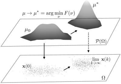
Figure 1: The figure illustrates scale separation in coverage control, with the agent positions in the domain $\Omega$ and the corresponding probability distributions over $\Omega$ constituting the microscopic and macroscopic representations, respectively.

3 Mathematical preliminaries

Here, we summarize mathematical notions that are needed as a background to the main results of the paper. For more details, we refer the reader to [7, 46] for more information as well as to the Appendix.

3.1 The Wasserstein space of probability measures

Let $\Omega$ be a compact subset of ^d, let $\mathcal{P}(\Omega)$ denote the space of probability measures over $\Omega$ and $\mathcal{P}^{\textup{a}}(\Omega)$ the set of atomless probability measures over $\Omega$. The $L^{2}$-Wasserstein distance between $\mu,\nu\in\mathcal{P}(\Omega)$ is given by:

$$W_{2}^{2}(\mu,\nu)=\min_{\pi\in\Pi(\mu,\nu)}\int_{\Omega\times\Omega}|x-y|^{2}~{}d\pi(x,y),$$ (2)

where $\Pi(\mu,\nu)$ is the space of joint probability measures over $\Omega\times\Omega$ with marginals $\mu$ and $\nu$. The definition of $L^{2}$-Wasserstein distance in (22) follows from the so-called Kantorovich formulation of optimal transport. An alternative formulation of this problem, called the Monge formulation of optimal transport, is given below:

$$W_{2}^{2}(\mu,\nu)=\min_{\begin{subarray}{c}T:\Omega\rightarrow\Omega\\ T_{\#}\mu=\nu\end{subarray}}\int_{\Omega}|x-T(x)|^{2}~{}d\mu(x).$$ (3)

In the Monge formulation (23), the minimization is carried out over the space of maps $T:\Omega\rightarrow\Omega$ for which the probability measure $\nu$ is obtained as the pushforward of $\mu$; i.e. $\mathcal{T}_{\#}\mu=\nu$. This can be viewed as a deterministic formulation of optimal transport, where the transport is carried out by a map, whereas the Kantorovich formulation (22) can be seen as a problem relaxation, where the transport plan is described by a joint probability measure $\pi$ over $\Omega\times\Omega$, with $\mu$ and $\nu$ as its marginals. It is to be noted that the Monge formulation does not always admit a solution, while the Kantorovich problem does. Roughly speaking, the Kantorovich formulation is the “minimal” extension of the Monge formulation, as both problems attain the same infimum. The result [46, Theorem 1.17] guarantees the existence and uniqueness of minimizers for both problems, when $\mu$ is atomless.

It holds that [7] that $(\mathcal{P}({\Omega}),W_{2})$ is a complete metric space. In addition, $W_{2}$ metrizes the convergence wrt the so-called weak topology (cf. [50, Theorem 6.9]). Due to this, we will indistinctively refer to convergence of measures in the weak topology as convergence wrt $W_{2}$. Finally, it can be shown that $\mathcal{P}({\Omega})$ is compact wrt the weak topology; see Appendix.

3.2 Regularity of functionals on the Wasserstein space

Results in convex analysis can be appropriately generalized to functionals on the $L^{2}$-Wasserstein space $(\mathcal{P}(\Omega),W_{2})$, see [1] for a detailed treatment. Before we can define any notion of convexity on $(\mathcal{P}(\Omega),W_{2})$, we need to introduce an appropriate notion of interpolation, which plays a similar role to the notion of segments in Euclidean space.

Definition 1 (Generalized displacement interpolation).

Let $\Omega$ be a compact subset of ^d, $\mu,\nu\in\mathcal{P}(\Omega)$, and $\theta\in\mathcal{P}^{\textup{a}}(\Omega)$ be an atomless probability measure. Let $T_{\theta\rightarrow\mu}:\Omega\rightarrow\Omega$ and $T_{\theta\rightarrow\nu}:\Omega\rightarrow\Omega$ be the optimal transport maps from $\theta$ to $\mu$, and $\theta$ to $\nu$ resp. in the $L^{2}$-Wasserstein space over $\Omega$. A (generalized) displacement interpolant of $\mu$ and $\nu$ w.r.t. $\theta$ is given by $\gamma_{t}=\left((1-t)T_{\theta\rightarrow\mu}+tT_{\theta\rightarrow\nu}\right)_{\#}\theta$, for $t\in[0,1]$.

We refer the reader to [1, Chapter 9.2] for a detailed discussion of the above notion and its motivation. It can be shown that, for a compact and convex $\Omega\subset^{d}$, the space $\mathcal{P}(\Omega)$ is geodesically convex w.r.t. the notion of generalized displacement interpolation for any absolutely continuous reference measure $\theta\in\mathcal{P}^{\textup{a}}(\Omega)$. Now, we introduce the following standard definition on the (generalized) geodesic convexity of functionals on the $L^{2}$-Wasserstein space $(\mathcal{P}(\Omega),W_{2})$. We note that this is a particular case of a more general definition of convexity in [1, Chapter 9] (Definition 9.2.4 for $\lambda=0$.)

Definition 2 ((Generalized) Geodesic convexity).

Let $\Omega\subseteq^{d}$ be a compact and convex set, and let $\mu,\nu,\theta\in\mathcal{P}^{\textup{a}}(\Omega)$ be atomless probability measures, for which there exist unique $T_{\theta\rightarrow\mu}:\Omega\rightarrow\Omega$ and $T_{\theta\rightarrow\nu}:\Omega\rightarrow\Omega$ optimal transport maps from $\theta$ to $\mu$ and from $\theta$ to $\nu$ respectively, in $(\mathcal{P}(\Omega),W_{2})$. A functional $F:\mathcal{P}(\Omega)\rightarrow$ is (generalized) geodesically convex w.r.t. $\theta\in\mathcal{P}(\Omega)$ (resp. (generalized) strictly geodesically convex w.r.t. $\theta$) if the following holds for every $t\in[0,1]$:

$$F(\left((1-t)T_{\theta\rightarrow\mu}+tT_{\theta\rightarrow\nu}\right)_{\#}\theta)\leq(1-t)F(\mu)+tF(\nu).$$

(resp. the previous inequality holds with strict inequality). Furthermore, a functional $F$ is geodesically convex (resp. strictly geodesically convex) if it is generalized geodesically convex (resp.strictly generalized geodesically convex) with respect to any atomless probability measure $\theta\in\mathcal{P}^{\textup{a}}(\Omega)$.

As in the finite-dimensional case, it can be shown that a geodesically convex functional is also continuous, thus, it admits a maximizer/minimizer over the compact $(\mathcal{P}(\Omega),W_{2})$. It is possible to obtain a first-order characterization of convexity for Fréchet differentiable functionals on atomless measures. The notion of Fréchet differential in Wasserstein space [1] is an extension of the standard notion for functions defined on ^d. For the sake of completeness, we provide a statement of the first-order convexity characterization:

Lemma 1 (First-order convexity condition).

Let $\Omega\subseteq^{d}$ be compact and convex, $\mu,\nu,\theta\in\mathcal{P}^{\textup{a}}(\Omega)$ be atomless measures. Let $F:\mathcal{P}(\Omega)\rightarrow$ be a Fréchet differentiable and (generalized) geodesically convex functional. Then, we have:

$$F(\nu)\geq F(\mu)+\int_{\Omega}\left\langle\xi_{\mu}(T_{\theta\rightarrow\mu}),T_{\theta\rightarrow\nu}-T_{\theta\rightarrow\mu}\right\rangle d\theta,$$ (4)

where $\xi_{\mu}$ is the Fréchet derivative of $F$ at $\mu$, and $T_{\theta\rightarrow\mu}:\Omega\rightarrow\Omega$ and $T_{\theta\rightarrow\nu}:\Omega\rightarrow\Omega$ are optimal transport maps from $\theta$ to $\mu$ and from $\theta$ to $\nu$ respectively.

Finally, we define the notion of strong geodesic convexity of Fréchet-differentiable functionals on $(\mathcal{P}(\Omega),W_{2})$:

Definition 3 (Strong geodesic convexity of a functional on $(\mathcal{P}(\Omega),W_{2})$).

Let $\Omega\subseteq^{d}$ be compact and convex and $\mu,\nu,\theta\in\mathcal{P}^{\textup{a}}(\Omega)$ be atomless probability measures. Let $F:\mathcal{P}(\Omega)\rightarrow$ be Frechét-differentiable. Let $\xi_{\mu}$ and $\xi_{\nu}$ be the Fréchet derivatives of $F$ evaluated at measures $\mu$ and $\nu$, respectively. Then, $F$ is strongly (geodesically) convex w.r.t. $\theta$ as reference measure if there exists an $m>0$ such that:

$$F(\nu) \geq F(\mu)+\int_{\Omega}\left\langle\xi_{\mu}(T_{\theta\rightarrow\mu}),T_{\theta\rightarrow\nu}-T_{\theta\rightarrow\mu}\right\rangle d\theta$$

$$\qquad+\frac{m}{2}\int_{\Omega}\left|T_{\theta\rightarrow\nu}-T_{\theta\rightarrow\mu}\right|^{2}d\theta,$$

where $T_{\theta\rightarrow\mu}$, $T_{\theta\rightarrow\nu}$ are the optimal transport maps from $\theta$ to $\mu$, $\nu$ respectively.

It can be shown that strong geodesic convexity of functionals implies strict geodesic convexity and, thus, geodesic convexity of functionals over $\mathcal{P}^{\textup{a}}(\Omega)$. It can also be proven that a Fréchet differentiable, strongly geodesically convex function admits a unique minimizer over $\mathcal{P}(\Omega)$.

Furthermore, we introduce the notion of $l$-smoothness that will be useful for the development of gradient descent-based transport schemes in the paper.

Definition 4 ($l$-smoothness of functionals on $(\mathcal{P}(\Omega),W_{2})$).

A functional $F:\mathcal{P}(\Omega)\rightarrow$ is called $l$-smooth w.r.t. a base measure $\theta\in\mathcal{P}^{\rm a}(\Omega)$ if for any $\mu,\nu\in\mathcal{P}^{\rm a}(\Omega)$, we have:

$$\left|F(\nu)-F(\mu)-\int_{\Omega}\left\langle\xi_{\mu}(T_{\theta\rightarrow\mu}),T_{\theta\rightarrow\nu}-T_{\theta\rightarrow\mu}\right\rangle d\theta\right|$$

$$\leq\frac{l}{2}\int_{\Omega}\left|T_{\theta\rightarrow\nu}-T_{\theta\rightarrow\mu}\right|^{2}d\theta,$$

where $\xi_{\mu}$ is the Fréchet derivative of $F$ evaluated at $\mu$, and $T_{\theta\rightarrow\mu}$, $T_{\theta\rightarrow\nu}$ are the optimal transport maps from $\theta$ to $\mu$, $\nu$ respectively.

4 Macroscopic and particle descent schemes

In this section, we present a (macroscopic) iterative descent scheme in the space of probability measures $\mathcal{P}(\Omega)$ and establish weak convergence to the minimizer under certain conditions. Furthermore, we derive an equivalent (microscopic) characterization of the descent scheme in $\Omega$. More specifically, Theorem 1 first establishes convergence of the proximal descent scheme (5) in $\mathcal{P}(\Omega)$ under appropriate conditions. In Theorem 2 we establish the microscopic scheme in $\Omega$ corresponding to (5). We then note the hurdle to implementation of the above scheme and circumvent it by an appropriate modification of the scheme and establish its convergence in Theorem 3. We refer to the Appendix for additional definitions and supporting results.

We consider the following proximal recursion in $\mathcal{P}(\Omega)$ starting from any absolutely continuous $\mu_{0}\in\mathcal{P}(\Omega)$:

$$\mu_{k+1}\in\arg\min_{\nu\in\mathcal{P}(\Omega)}\frac{1}{2\tau}W_{2}^{2}(\mu_{k},\nu)+F(\nu).$$ (5)

In the remainder of this section, we will assume that $F$ is sufficiently regular, which ensures that the previous scheme is well defined and results in an atomless sequence of measures with negligible mass on $\partial\Omega$.

Assumption 1 (Regularity conditions on $F$).

The functional $F:\mathcal{P}(\Omega)\rightarrow$ is $l$-smooth (in the sense of Definition 4 w.r.t. any base measure $\theta\in\mathcal{P}^{\rm a}(\Omega)$) and strictly geodesically convex on $(\mathcal{P}(\Omega),W_{2})$ (in the sense of Definition 2 w.r.t. any base measure $\theta\in\mathcal{P}^{\rm a}(\Omega)$). The Fréchet derivative $\xi_{\mu}$ of $F$ is Lipschitz continuous on $\Omega$ (with Lipschitz constant $\lambda$) at any $\mu\in\mathcal{P}^{\rm a}(\Omega)$. Furthermore, it satisfies the boundary condition $\xi_{\mu}\cdot\mathbf{n}\geq 0$ on $\partial\Omega$ (where $\mathbf{n}$ is the outward normal to $\partial\Omega$) for any $\mu\in\mathcal{P}^{\rm a}(\Omega)$.

Assumption 2 (Atomless proximal descent sequence).

We assume that the sequence $\{\mu_{k}\}_{k\in\mathbb{N}}$ generated by (5) is such that $\mu_{k}\in\mathcal{P}^{\textup{a}}(\Omega)$ for all $k\in\mathbb{N}$.

We remark here that sufficient regularity of the functional $F$ and the atomlessness of $\mu_{0}$ should guarantee validity of Assumption 2. Since we do not offer a characterization of the regularity of $F$ to this end, we retain Assumption 2 in establishing the following theorem:

Theorem 1 (Convergence of proximal recursion (5)).

Let $\Omega\subseteq^{d}$ be a compact, convex set, and let $F:\mathcal{P}(\Omega)\rightarrow$ satisfy the regularity conditions of Assumption 1. Let $\mu_{0}$ be an absolutely continuous measure. Under Assumption 2 on the generation of a proximal descent atomless sequence, and for $0<\tau<1/l$, the sequence $\{\mu_{k}\}_{k\in\mathbb{N}}$, generated by the proximal recursion (5), converges weakly to $\mu^{\star}=\arg\min_{\nu\in\mathcal{P}(\Omega)}F(\nu)$ as $k\rightarrow\infty$.

Proof.

It follows that:

$$\frac{1}{2\tau}W_{2}^{2}(\mu_{k},\mu_{k+1})+F(\mu_{k+1})\leq F(\mu_{k})$$

$$\Longleftrightarrow F(\mu_{k+1})\leq F(\mu_{k})-\frac{1}{2\tau}W_{2}^{2}(\mu_{k},\mu_{k+1}).$$

This implies that for $\mu_{k}\neq\mu_{k+1}$, we have $F(\mu_{k+1})<F(\mu_{k})$ and the sequence $\{F(\mu_{k})\}_{k\in\mathbb{N}}$ is monotonically strictly decreasing. In addition, $\{\mu_{k}\}_{k\in\mathbb{N}}$ is contained in the sublevel set $\mathcal{S}(\mu_{0})$ of $F(\mu_{0})$.

From Lemma 16 in the Appendix, $\mathcal{S}(\mu_{0})$ is geodesically convex and compact in the $L^{2}$-Wasserstein space $(\mathcal{P}(\Omega),W_{2})$. Thus, there is a weakly convergent subsequence $\{\mu_{k_{\ell}}\}\rightarrow_{\ell}\overline{\mu}\in\mathcal{S}(\mu_{0})$. Consider the functional $G_{\mu}$ from (5), for $\mu\in\mathcal{P}(\Omega)$, such that $G_{\mu}(\nu)=\frac{1}{2\tau}W_{2}^{2}(\mu,\nu)+F(\nu)$. First, note that

$$|G_{\mu_{k_{\ell}}}(\nu)-G_{\overline{\mu}}(\nu)|=\frac{1}{2\tau}|W_{2}^{2}(\overline{\mu},\nu)-W_{2}^{2}(\mu_{k_{\ell}},\nu)|$$

$$=\frac{1}{2\tau}(W_{2}(\overline{\mu},\nu)+W_{2}(\mu_{k_{\ell}},\nu))|W_{2}(\overline{\mu},\nu)-W_{2}(\mu_{k_{\ell}},\nu)|,$$

for all $\ell$. Due to the triangular inequality, for all $\nu$, $|W_{2}(\overline{\mu},\nu)-W_{2}(\mu_{k_{\ell}},\nu)|\leq W_{2}(\mu_{k_{\ell}},\overline{\mu})$. Therefore,

$$|G_{\mu_{k_{\ell}}}(\nu)-G_{\overline{\mu}}(\nu)|\leq\frac{1}{2\tau}(W_{2}(\overline{\mu},\nu)+W_{2}(\mu_{k_{\ell}},\nu))W_{2}(\overline{\mu},\mu_{k_{\ell}}).$$

In addition, $\mathcal{S}(\mu_{0})$ is a compact set and $W_{2}$ is a continuous functional, then there is a constant $M$ such that $W_{2}(\overline{\mu},\nu)+W_{2}(\mu_{k_{\ell}},\nu)\leq M$ and we have:

$$|G_{\mu_{k_{\ell}}}(\nu)-G_{\overline{\mu}}(\nu)|\leq\frac{M}{2\tau}W_{2}(\overline{\mu},\mu_{k_{\ell}}),$$

for all $\nu$. Since $\mu_{k_{\ell}}\rightarrow_{\ell}\overline{\mu}$, this implies the uniform convergence of the functionals $G_{\mu_{k_{\ell}}}(\nu)$ to $G_{\overline{\mu}}(\nu)$. In particular, this implies that for all $\epsilon>0$, there is an $\ell_{0}$ such that for all $\ell\geq\ell_{0}$, we have

$$|G_{\mu_{k_{\ell}}}(\nu)-G_{\overline{\mu}}(\nu)|<\epsilon,$$

for all $\nu$. Let $\overline{\mu}^{+}=\arg\min_{\nu}G_{\overline{\mu}}(\nu)$, and recall that $\mu_{k_{\ell}+1}=\arg\min_{\nu}G_{\mu_{k_{\ell}}}(\nu)$. Then, by the $\min$ properties:

$$G_{\mu_{k_{\ell}}}(\mu_{k_{\ell}+1})\leq G_{\mu_{k_{\ell}}}(\nu)<G_{\overline{\mu}}(\nu)+\epsilon$$

$$\quad\qquad\Longrightarrow\,G_{\mu_{k_{\ell}}}(\mu_{k_{\ell}+1})\leq G_{\overline{\mu}}(\overline{\mu}^{+})+\epsilon,$$

$$G_{\overline{\mu}}(\overline{\mu}^{+})-\epsilon<G_{\overline{\mu}}(\nu)-\epsilon\leq G_{\mu_{k_{\ell}}}(\nu)$$

$$\quad\qquad\Longrightarrow\,G_{\overline{\mu}}(\overline{\mu}^{+})-\epsilon\leq G_{\mu_{k_{\ell}}}(\mu_{k_{\ell}+1}).$$

That is, we have $|G_{\mu_{k_{\ell}}}(\mu_{k_{\ell}+1})-G_{\overline{\mu}}(\overline{\mu}^{+})|\leq\epsilon$ for all $\ell\geq\ell_{0}$. The fact that $\overline{\mu}$ is a fixed point for $G_{\overline{\mu}}(\nu)$ now follows from the set of inequalities:

$$G_{\overline{\mu}}(\overline{\mu}^{+})\leq G_{\overline{\mu}}(\overline{\mu})=F(\overline{\mu})\leq G_{\mu_{k_{\ell}}}(\mu_{k_{\ell}+1})<F(\mu_{k_{\ell}})$$

The gap $G_{\mu_{k_{\ell}}}(\mu_{k_{\ell}+1})-G_{\overline{\mu}}(\overline{\mu}^{+})$ can be made arbitrarily small by increasing $\ell$, so it must be that $G_{\overline{\mu}}(\overline{\mu})=F(\overline{\mu})=G_{\overline{\mu}}(\overline{\mu}^{+})$, which implies $\overline{\mu}^{+}=\overline{\mu}$ is the solution to the minimization problem of $G_{\overline{\mu}}$ and satisfies $\nabla\left(\frac{\delta G}{\delta\nu}\right)_{\overline{\mu}}=0$. The equation $\nabla\left(\frac{\delta G}{\delta\nu}\right)_{\overline{\mu}}=0$ is equivalent to $\frac{1}{\tau}\nabla\phi_{\overline{\mu}\rightarrow\overline{\mu}}+\nabla\left(\frac{\delta F}{\delta\nu}\right)_{\overline{\mu}}=0$. Since $\nabla\phi_{\overline{\mu}\rightarrow\overline{\mu}}=0$, then $\overline{\mu}$ is a minimizer of $F$, and from the strict geodesic convexity of $F$ we get that the minimizer is unique and $\overline{\mu}=\mu^{\star}$. Note that we can apply this reasoning to all the accumulation points $\tilde{\mu}$ of the sequence $\{\mu_{k}\}$. Since all the convergent subsequences of $\{\mu_{k}\}$ have the same limit $\mu^{\star}$ and $\{\mu_{k}\}$ is contained in $\mathcal{S}(\mu_{0})$ which is compact, we conclude that the whole sequence $\{\mu_{k}\}$ converges to $\mu^{\star}$ in $W_{2}$, i.e., weakly as $k\rightarrow\infty$. $\square$∎

Remark 1 (Squared-Wasserstein distance as objective functional).

We now consider the case where the $L^{2}$-Wasserstein distance from the target measure $\mu^{*}$ is chosen as the objective functional, i.e., $F(\nu)=\frac{1}{2}W_{2}^{2}(\nu,\mu^{*})$. We note that $F$ is strictly (generalized) geodesically convex only w.r.t. $\mu^{*}$ as the reference measure. This violates the regularity assumption 1 (where we let $F$ to be strictly (generalized) geodesically convex w.r.t. any (atomless) reference measure) and presentes a hurdle to the application of Theorem 1. However, this hurdle can be mitigated as follows. Let $G_{\mu_{k}}(\nu)=\frac{1}{2\tau}W_{2}^{2}(\mu_{k},\nu)+F(\nu)$. The Fréchet derivative of $G_{\mu_{k}}$ is given by $\nabla\left(\left.\frac{\delta G_{\mu_{k}}(\nu)}{\delta\nu}\right|_{\nu}\right)=\frac{1}{\tau}\nabla\phi_{\nu\rightarrow\mu_{k}}+\nabla\phi_{\nu\rightarrow\mu^{*}}$. Moreover, at the critical point $\mu_{k+1}$ of $G_{\mu_{k}}$ we have $\frac{1}{\tau}\nabla\phi_{\mu_{k+1}\rightarrow\mu_{k}}+\nabla\phi_{\mu_{k+1}\rightarrow\mu^{*}}=\frac{1}{\tau}\left(\operatorname{id}-T_{\mu_{k+1}\rightarrow\mu_{k}}\right)+\left(\operatorname{id}-T_{\mu_{k+1}\rightarrow\mu^{*}}\right)=0$, which implies that $\left(T_{\mu_{k+1}\rightarrow\mu_{k}}-\operatorname{id}\right)=\tau\left(\operatorname{id}-T_{\mu_{k+1}\rightarrow\mu^{*}}\right)$. We then have $W_{2}(\mu_{k},\mu_{k+1})=\tau W_{2}(\mu_{k+1},\mu^{*})$. For any (and only) $\nu$ on the geodesic between $\mu_{k}$ and $\mu^{*}$, we have $W_{2}(\mu_{k},\mu^{*})=W_{2}(\mu_{k},\nu)+W_{2}(\nu,\mu^{*})$ (wherein the triangle inequality is an equality), and this is the case if and only if $\int_{\Omega}\left\langle\operatorname{id}-T_{\nu\rightarrow\mu_{k}},T_{\nu\rightarrow\mu^{*}}-\operatorname{id}\right\rangle d\nu=W_{2}(\mu_{k},\nu)W_{2}(\nu,\mu^{*})$. We see that this is indeed the case for $\nu=\mu_{k+1}$, from which we infer that $\mu_{k+1}$ lies on the geodesic between $\mu_{k}$ and $\mu^{*}$. We therefore get that $\{\mu_{k}\}_{k\in\mathbb{N}}$ lies on the geodesic connecting $\mu_{0}$ and $\mu^{*}$. Consequently, need only be concerned with the geodesic convexity of $F$ along the geodesic connecting $\mu_{0}$ and $\mu^{*}$. Now, from Proposition 2 in Appendix F it follows that $W_{2}^{2}(\cdot,\mu_{k})$ is generalized geodesically convex with reference measure $\mu_{k}$, and similarly $W_{2}^{2}(\cdot,\mu^{*})$ is generalized geodesically convex with reference measure $\mu^{*}$, and the two measures $\mu_{k}$ and $\mu^{*}$ are interchangeable as reference measures along the geodesic between them. It then follows that $\mu_{k}$ can be chosen as the reference measure and the arguments in the proof of Theorem 1 apply.

The implementation of (5) can be challenging because involves the solution of an infinite-dimensional optimization problem. To address this, we determine the stochastic process in $\Omega$ that equivalently describes the recursion (5). More precisely, consider a proximal recursion in $\Omega$ from an initial condition $x_{0}\in\Omega$:

$$x_{k+1}\in\arg\min_{z\in\Omega}\frac{1}{2\tau}|x_{k}-z|^{2}+f_{k}(z),$$ (6)

where $\{f_{k}\}_{k\in\mathbb{N}}$ is a sequence of functions on $\Omega$. Suppose that the initial condition $x_{0}$ is in fact a random variable distributed according to $\mu_{0}$ (denoted $x_{0}\sim\mu_{0}$). We are interested in defining the process in $\Omega$, through an appropriate choice of $\{f_{k}\}_{k\in\mathbb{N}}$, which results in a consistent transport of the initial measure $\mu_{0}$ according to the recursion (5).

Theorem 2 (Target dynamics in $\Omega$).

Let $\Omega\subseteq^{d}$ be a compact, convex set, and let $F:\Omega\longrightarrow$ satisfy the regularity conditions of Assumption 1. Under Assumption 2, the proximal recursion (5), for $0<\tau<1/l$, starting from $\mu_{0}\in\mathcal{P}^{a}(\Omega)$ is obtained as the transport of $\mu_{0}$ by (6) with $x_{0}\sim\mu_{0}$ and $f_{k}=\left.\frac{\delta F}{\delta\nu}\right|_{\mu_{k+1}}$, for all $k\in\mathbb{N}$.

Proof.

We rewrite the single-step update in (5) from an absolutely continuous probability measure $\mu\in\mathcal{P}(\Omega)$ as follows:

$$\mu^{+}=\arg\min_{\nu\in\mathcal{P}(\Omega)}\frac{1}{2\tau}W_{2}^{2}(\mu,\nu)+F(\nu).$$ (7)

From Lemma 17 the minimizer $\mu^{+}$ in (7) is unique. Let $\{\mathbf{v}_{\epsilon}\}$ be a smooth one-parameter family of Lipschitz continuous vector fields such that $\mathbf{v}_{0}=\mathbf{v}$, where $\mathbf{v}$ is any Lipschitz vector field on $\Omega$. Now, define a one-parameter family of absolutely continuous probability measures $\{\nu_{\epsilon}\}_{\epsilon\in}$ by means of $\partial_{\epsilon}\nu_{\epsilon}+\nabla\cdot(\nu_{\epsilon}\mathbf{v}_{\epsilon})=0$, subject to $\mathbf{v}_{\epsilon}\cdot\mathbf{n}=0$, and such that $\nu_{0}=\mu^{+}$. Since $\mu^{+}$ is a critical point of the objective function in (7), from [46, Theorem 5.24] we have:

$$0 =\left.\frac{d}{d\epsilon}\left(\frac{1}{2\tau}W_{2}^{2}(\mu,\nu_{\epsilon})+F(\nu_{\epsilon})\right)\right|_{\epsilon=0}$$

$$=\frac{1}{\tau}\int_{\Omega}\left\langle\nabla\phi_{\mu^{+}\rightarrow\mu},\mathbf{v}\right\rangle d\mu^{+}+\int_{\Omega}\left\langle\xi,\mathbf{v}\right\rangle d\mu^{+}$$

$$=\int_{\Omega}\left\langle\frac{1}{\tau}\nabla\phi_{\mu^{+}\rightarrow\mu}+\xi,\mathbf{v}\right\rangle d\mu^{+},$$

where $\xi=\left.\nabla\left(\frac{\delta F}{\delta\nu}\right)\right|_{\nu=\mu^{+}}$ and $\nabla\phi_{\mu^{+}\rightarrow\mu}=\operatorname{id}-T_{\mu^{+}\rightarrow\mu}$, with $T_{\mu^{+}\rightarrow\mu}:\Omega\rightarrow\Omega$ being the optimal transport map from $\mu^{+}$ to $\mu$. Since $\int_{\Omega}\left\langle\frac{1}{\tau}\nabla\phi_{\mu^{+}\rightarrow\mu}+\xi,\mathbf{v}\right\rangle d\mu^{+}=0$ for all $\mathbf{v}$, it implies that $\frac{1}{\tau}\nabla\phi_{\mu^{+}\rightarrow\mu}+\xi=0$ ($\mu^{+}$ a.e. in $\Omega$), and we obtain:

$$\frac{1}{\tau}\nabla\phi_{\mu^{+}\rightarrow\mu}+\xi=\frac{1}{\tau}\left(\operatorname{id}-T_{\mu^{+}\rightarrow\mu}\right)+\xi=0,$$

which implies that:

$$T_{\mu^{+}\rightarrow\mu}=\operatorname{id}+\tau\xi.$$ (8)

Let $\varphi=\left.\left(\frac{\delta F}{\delta\nu}\right)\right|_{\nu=\mu^{+}}$. For any $y\in\Omega$ and $\tau<1/l$, consider:

$$y^{+}=\arg\min_{z\in\Omega}\underbrace{\frac{1}{2\tau}|y-z|^{2}+\varphi(z)}_{\triangleq g_{y}(z)}.$$ (9)

The uniqueness of the minimizer above follows from the strong convexity of $g_{y}$ for $\tau<1/l$ (this can be verified by following a similar procedure as in the proof of Lemma 17, but now in the Euclidean space). If $y^{+}\in\mathring{\Omega}$ is a critical point of $g_{y}$ in (9), then it satisfies $y^{+}=y-\tau\nabla\varphi(y^{+})$. Since $\xi=\nabla\varphi$, we can equivalently write $y^{+}=\left(\operatorname{id}+\tau\xi\right)^{-1}(y)$. That is, when the image of $y\in\Omega$ under the $\arg\min$ map in (9) is a critical point in the interior of $\Omega$, then it is also the inverse image of $y$ under the optimal transport map $T_{\mu^{+}\rightarrow\mu}$.

Now, for a $y\in\mathring{\Omega}$, the inner product of the gradient of $g_{y}$ at any point $z\in\partial\Omega$ on the boundary of $\Omega$ with the outward normal $\mathbf{n}$ to $\partial\Omega$ at $z$ is given by $\nabla g_{y}\cdot\mathbf{n}=\left(\frac{1}{\tau}(z-y)+\nabla\varphi(z)\right)\cdot\mathbf{n}=\frac{1}{\tau}(z-y)\cdot\mathbf{n}>0$, since $\nabla\varphi\cdot\mathbf{n}=0$ and $z-y$ points outward to $\Omega$ (as $z\in\partial\Omega$ and $y\in\mathring{\Omega}$ and $\Omega$ is convex). This implies that there exists a point $\tilde{z}$ in the interior of $\Omega$ in a neighborhood of $z$ such that $g_{y}(\tilde{z})<g_{y}(z)$, which implies that $z$ cannot be the minimizer. Thus, for any $y\in\mathring{\Omega}$, the minimizer of $g_{y}(z)=\frac{1}{2\tau}|y-z|^{2}+\varphi(z)$ cannot lie on the boundary $\partial\Omega$, and must therefore lie in the interior of $\Omega$ and be a critical point of the objective function $g_{y}$. Now, when $y\in\partial\Omega$, if $y^{+}\notin\mathring{\Omega}$, it must be that $y^{+}=y$ (otherwise we obtain a contradiction for the same reason as above, the inner product of $\nabla g_{y}$ with the outward normal would be strictly positive) and the $\mathrm{argmin}$ map (and the optimal transport map) coincides with the identity map in this case.

It then follows that for any $y\in\Omega$, its image $y^{+}$ under the $\mathrm{argmin}$ map is exactly its inverse image under the optimal transport map $T_{\mu^{+}\rightarrow\mu}$. That is, the map in (9) is the inverse of the optimal transport map $T_{\mu^{+}\rightarrow\mu}$. Thus, we have that the map $T_{\mu^{+}\rightarrow\mu}=\operatorname{id}+\tau\xi$ is well-defined and so is its inverse, it holds that $\left(T_{\mu^{+}\rightarrow\mu}\right)^{-1}_{\#}\mu=\left(\operatorname{id}+\tau\xi\right)^{-1}_{\#}\mu=\mu^{+}$, and (7) is the lift to the space of probability measures of (9).

We therefore conclude that the proximal recursion (5) starting from $\mu_{0}$ is the transport of $\mu_{0}$ by (6) with $x_{0}\sim\mu_{0}$. $\square$∎

From a computational perspective, Theorem 2 still requires the evaluation of the first variation $\frac{\delta F}{\delta\nu}$ at $\mu_{k+1}$, the transported measure at the future time instant $k+1$. To circumvent this problem, we can alternatively consider the dynamics (6) with the choice of $\tilde{f}_{k}=\left.\frac{\delta F}{\delta\nu}\right|_{\mu_{k}}$, which only requires the evaluation, at time instant $k$, of the first variation $\frac{\delta F}{\delta\nu}$ at $\mu_{k}$. Consider the $l$-smooth, geodesically-convex (linear) $\widetilde{F}(\nu)=\mathbb{E}_{\nu}\left[\left.\frac{\delta F}{\delta\mu}\right|_{\mu_{k}}\right]$, for $\nu\in\Omega$, which satisfies $\frac{\delta\widetilde{F}}{\delta\nu}=\left.\frac{\delta F}{\delta\mu}\right|_{\mu_{k}}$. It follows from Theorem 2 that the descent in $\mathcal{P}(\Omega)$ corresponding to (6) with $\tilde{f}_{k}=\left.\frac{\delta\widetilde{F}}{\delta\nu}\right|_{\mu_{k}}$ is given by:

$$\mu_{k+1}\in\arg\min_{\nu\in\mathcal{P}(\Omega)}\frac{1}{2\tau}W_{2}^{2}(\mu_{k},\nu)+\mathbb{E}_{\nu}\left[\left.\frac{\delta F}{\delta\mu}\right|_{\mu_{k}}\right].$$ (10)

The convergence of (10) can also be established as follows:

Theorem 3 (Convergence of recursion (10)).

Let $F:\Omega\rightarrow$ satisfy the regularity conditions of Assumption 1 and let $\alpha=l+\lambda$. The sequence $\{\mu_{k}\}_{k\in\mathbb{N}}$ obtained as the transport of measure $\mu_{0}\in\mathcal{P}^{a}(\Omega)$ by (10) with $\tau<1/\alpha$, $x_{0}\sim\mu_{0}$ and the choice $\tilde{f}_{k}=\left.\frac{\delta\widetilde{F}}{\delta\nu}\right|_{\mu_{k}}$, converges weakly to $\mu^{\star}=\arg\min_{\nu\in\mathcal{P}(\Omega)}F(\nu)$ as $k\rightarrow\infty$.

Proof.

From the $l$-smoothness of $F$ and Lemma 15 (with $\mu_{k+1}$ as the reference measure), we get:

$$\int_{\Omega}\left\langle\xi_{k}(T_{\mu_{k+1}\rightarrow\mu_{k}})-\xi_{k+1},T_{\mu_{k+1}\rightarrow\mu_{k}}-\operatorname{id}\right\rangle d\mu_{k+1}$$

$$\leq lW_{2}^{2}(\mu_{k},\mu_{k+1}).$$

Since $\mathbb{E}_{\nu}\left[\left.\frac{\delta F}{\delta\mu}\right|_{\mu_{k}}\right]$ is linear in $\nu$ for a given $\mu_{k}$, and the Fréchet derivative of $F$ is Lipschitz continuous at any atomless probability measure (with Lipschitz constant $\lambda$), it follows from Lemma 17 that the objective functional in (10) is strongly convex w.r.t. reference measure $\mu_{k}$ (note that $\tau<1/\alpha=1/(l+\lambda)<1/\lambda$), and therefore has a unique minimizer. Following similar steps as in the proof of Theorem 1 to characterize the critical point of (10), we get that $T_{\mu_{k+1}\rightarrow\mu_{k}}=\operatorname{id}+\tau\xi_{k}$, and by substitution in the above, we obtain:

$$\int_{\Omega}\left\langle\xi_{k+1},T_{\mu_{k+1}\rightarrow\mu_{k}}-\operatorname{id}\right\rangle d\mu_{k+1}$$

$$\geq\int_{\Omega}\left\langle\xi_{k}(T_{\mu_{k+1}\rightarrow\mu_{k}}),T_{\mu_{k+1}\rightarrow\mu_{k}}-\operatorname{id}\right\rangle d\mu_{k+1}$$

$$\qquad\qquad-lW_{2}^{2}(\mu_{k},\mu_{k+1})$$

$$=\int_{\Omega}\left\langle\xi_{k}(T_{\mu_{k+1}\rightarrow\mu_{k}})-\xi_{k},T_{\mu_{k+1}\rightarrow\mu_{k}}-\operatorname{id}\right\rangle d\mu_{k+1}$$

$$\qquad+\int_{\Omega}\left\langle\xi_{k},T_{\mu_{k+1}\rightarrow\mu_{k}}-\operatorname{id}\right\rangle d\mu_{k+1}$$

$$\qquad\qquad-lW_{2}^{2}(\mu_{k},\mu_{k+1})$$

$$\geq-\lambda W_{2}^{2}(\mu_{k},\mu_{k+1})+\frac{1}{\tau}W_{2}^{2}(\mu_{k},\mu_{k+1})$$

$$\qquad\qquad-lW_{2}^{2}(\mu_{k},\mu_{k+1})$$

$$=\left(\frac{1}{\tau}-\alpha\right)W_{2}^{2}(\mu_{k},\mu_{k+1}).$$

Moreover, from the convexity of $F$ and Lemma 1 (with $\mu_{k+1}$ as the reference measure) we have:

$$F(\mu_{k})\geq F(\mu_{k+1})+\int_{\Omega}\left\langle\xi_{k+1},T_{\mu_{k+1}\rightarrow\mu_{k}}-\operatorname{id}\right\rangle d\mu_{k+1}.$$

Substituting in the latest inequality, we obtain:

$$F(\mu_{k})\geq F(\mu_{k+1})+\left(\frac{1}{\tau}-\alpha\right)W_{2}^{2}(\mu_{k},\mu_{k+1}).$$

From this inequality, we deduce that $\mu_{k+1}$ belongs to the $F$-sublevel set of $\mu_{k}$, and consequently that the sequence $\{\mu_{k}\}_{k\in\mathbb{N}}$ is contained in $\mathcal{S}(\mu_{0})$, the $F$-sublevel set of $\mu_{0}$. From here, following similar steps as in the proof of Theorem 1, we conclude that the sequence $\{\mu_{k}\}_{k\in\mathbb{N}}$ is convergent and $\lim_{K\rightarrow\infty}W_{2}^{2}(\mu_{K},\bar{\mu})=0$ for some $\bar{\mu}\in\mathcal{S}(\mu_{0})$. As the sequence $\{\mu_{k}\}_{k\in\mathbb{N}}$ is generated by (10), the limit $\bar{\mu}$ must be one of its fixed points, again following similar reasoning as in Theorem 1. Since $F$ is strictly convex, we get that the only fixed point of (10) is $\mu^{\star}$. We therefore have $\bar{\mu}=\mu^{\star}$. $\square$∎

Now Theorem 2 allows us to consider the transport in $\mathcal{P}(\Omega)$ given by the following proximal scheme in $\Omega$:

$$x^{+}=\arg\min_{z\in\Omega}\frac{1}{2\tau}|x-z|^{2}+f(z),$$ (11)

where $x\sim\mu$ and $f=\left.\frac{\delta F}{\delta\nu}\right|_{\mu}$. This scheme is convergent according to Theorem 3.

5 Multi-agent proximal descent algorithms

In this section, we bring the sample-based, proximal descent schemes of the previous section to a form that is closer to the more familiar multi-agent cooperative control algorithms. We achieve this by a direct discretization of the functional. By doing so, we are able to retain some convergence properties of the algorithms, as shown in this section. We then show that, in the limit of space and time discretizations, the corresponding algorithm recovers the lost properties.

We start by describing the multi-agent system by an appropriate probability distribution. Recall that the configuration of the collective is given by $\mathbf{x}=(x_{1},\ldots,x_{N})$, with $x_{i}\in\Omega$ for $i\in\{1,\ldots,N\}$. Let $\widehat{\mu}^{N}_{\mathbf{x}}=\frac{1}{N}\sum_{i=1}^{N}\delta_{x_{i}}$ be the discrete measure in $\mathcal{P}(\Omega)$ corresponding to the configuration $\mathbf{x}$, where $\delta_{x_{i}}$ is the Dirac measure supported at $x_{i}$. For a macroscopic description of the transport, we first let the macroscopic configuration be specified by an absolutely continuous probability measure, and since $\widehat{\mu}^{N}_{\mathbf{x}}$ is is not absolutely continuous, we consider an alternative absolutely continuous probability measure $\widehat{\mu}^{h,N}_{\mathbf{x}}$ through its density function using a smooth kernel, as follows:

$$\widehat{\mu}^{h,N}_{\mathbf{x}}(x)=\frac{1}{N}\sum_{i=1}^{N}K_{h}(x-x_{i}),$$ (12)

where $h>0$ is the bandwidth of the kernel. With a slight abuse of notation, we allow $\widehat{\mu}^{h,N}_{\mathbf{x}}$ to denote both the absolutely continuous measure and its corresponding density function. We also denote, for $x\in\Omega$, $\widehat{\mu}^{h,1}_{x}$ simply by $\widehat{\mu}^{h}_{x}$. Thus, we have $\widehat{\mu}^{h,N}_{\mathbf{x}}=\frac{1}{N}\sum_{i=1}^{N}\widehat{\mu}^{h}_{x_{i}}$, for $\mathbf{x}\in\Omega^{N}$.

Assumption 3 (Properties of kernel and kernel-based measures).

For $h>0$ and $z\in\Omega$ and a kernel-based probability measure $\widehat{\mu}^{h}_{z}$ defined as in (12) for $N=1$, the following hold:
(i) Smoothness: The kernel $K_{h}$ is smooth, $K_{h}\in C^{\infty}(\Omega)$, for every $h>0$.
(ii) Monotonicity of support: For any $z\in\Omega$ and $h_{1}<h_{2}$, we let $\operatorname{supp}\left(\widehat{\mu}^{h_{1}}_{z}\right)\subset\operatorname{supp}\left(\widehat{\mu}^{h_{2}}_{z}\right)$.
(iii) Containment: For every $h>0$, there exists a set $\tilde{\Omega}_{h}\subset\Omega$ (relatively) open, such that for $z\in\tilde{\Omega}_{h}$, the support of the measure $\widehat{\mu}^{h}_{z}$ satisfies $\operatorname{supp}(\widehat{\mu}^{h}_{z})\subset\Omega$. Moreover, $\lim_{h\rightarrow 0}\tilde{\Omega}_{h}=\Omega$ in Hausdorff distance.
(iv) Total variation convergence: Let $\mathcal{M}$ be the space of all measureable functions over $\Omega$. It holds that $\lim_{h\rightarrow 0}\sup_{f\in\mathcal{M}}\left\{\int_{\Omega}f(z)K_{h}(x-z)\operatorname{dvol}(z)-f(x)\right\}=0$, that is, the kernel-based measure converges uniformly to the Dirac measure as $h\rightarrow 0$.

An example kernel for (12) that satisfies Assumption 3 is the truncated Gaussian kernel restricted to an open ball $B_{h}(x_{i})$ of radius $h$ centered at $x_{i}$, given by $K_{h}(x-x_{i})=\frac{1}{C}\text{exp}\left(\frac{-\left|x-x_{i}\right|^{2}}{2h^{2}}\right)\mathbf{1}_{B_{h}(x_{i})}(x)$, where $C=\int_{B_{h}(x_{i})}\text{exp}\left(\frac{-\left|x-x_{i}\right|^{2}}{2h^{2}}\right)\operatorname{dvol}(x)$ is the normalizing constant.

5.1 Discretization of functional $F$ and its properties

We define an aggregate objective function $F^{h,N}$ for the multi-agent system as the discretization of the functional $F$, for $h>0$, as follows:

$$F^{h,N}(\mathbf{x})=F(\widehat{\mu}^{h,N}_{\mathbf{x}}),$$ (13)

and, subsequently, analyze its properties. First note that $F^{h,N}$ is invariant under permutations, that is, for $\mathbf{x}\in\tilde{\Omega}^{N}_{h}$ and $P\in^{N\times N}$ a permutation, we have $F^{h,N}(\mathbf{x})=F^{h,N}((P\otimes I_{d})~{}\mathbf{x})$. The following lemma establishes the almost sure convergence of the $F^{h,N}$ to $F$ as $h\rightarrow 0,N\rightarrow\infty$:

Lemma 2 (Convergence as $h\rightarrow 0,~{}N\rightarrow\infty$).

Let Assumption 3 and the Fréchet differentiability of the functional $F$ hold, and let $x_{i}\sim\mu$ for $i\in\{1,\dots,N\}$, independent and identically distributed. Then, we have $\lim_{h\rightarrow 0}\lim_{N\rightarrow\infty}F^{h,N}(x_{1},\ldots,x_{N})=F(\mu)$, $\mu$-almost surely.

The following lemma relates the derivative of the function $F^{h,N}$ to the Fréchet derivative of the functional $F$:

Lemma 3 (Derivative of $F^{h,N}$).

Let Assumption 3 and the Fréchet differentiability of the functional $F$ hold, and let $h>0$ with set $\tilde{\Omega}_{h}$ as in Assumption 3-(iii). For $\mathbf{x}=(z,\eta)\in\tilde{\Omega}_{h}\times\tilde{\Omega}_{h}^{N-1}$, we have that the derivative of the function $F^{h,N}$ satisfies:

$$\partial_{1}F^{h,N}(z,\eta)=\frac{1}{N}\int_{\operatorname{supp}\left(\widehat{\mu}^{h}_{z}\right)}\nabla\varphi^{h,N}_{\mathbf{x}}~{}d\widehat{\mu}^{h}_{z},$$

where $d\widehat{\mu}^{h}_{z}=\rho^{h}_{z}~{}\operatorname{dvol}$ with $\rho^{h}_{z}(x)=K(x-z,h)$, $\varphi^{h,N}_{\mathbf{x}}=\frac{\delta F}{\delta\nu}\left.\right|_{\widehat{\mu}^{h,N}_{\mathbf{x}}}$ and $\partial_{1}$ denotes the derivative w.r.t the first argument.

From the invariance of $F^{h,N}$ under permutations, the expression in Lemma 3 holds for the partial derivative of $F^{h,N}$ w.r.t every component of $\mathbf{x}$. In what follows, we will make the following assumption characterize the behavior of the discretization $F^{h,N}$ along the boundary through the following assumption:

Assumption 4 (Boundary conditions).

The function $F^{h,N}$ is Fréchet differentiable and its derivative satisfies the boundary condition $\partial_{1}F^{h,N}(z,\xi)\cdot\mathbf{n}(z)=0$ for $z\in\partial\tilde{\Omega}_{h}$ and all $\xi\in\tilde{\Omega}^{N-1}_{h}$.

In general, note that $F^{h,N}:\Omega^{N}\rightarrow$ is nonconvex in spite of being the discretization of a strictly geodesically convex functional $F:\mathcal{P}(\Omega)\rightarrow$. This is because the notion of convexity of functions over $\Omega^{N}$, which is the domain of the function $F^{h,N}$, is not implied by the notion of geodesic convexity over the space of probability measures over $\Omega$. In this way, for $\mathbf{x},\mathbf{y}\in\Omega^{N}$ with $\sum_{i=1}^{N}\frac{1}{N}\delta_{x_{i}},\sum_{i=1}^{N}\frac{1}{N}\delta_{y_{i}}\in\mathcal{P}(\Omega)$ being the corresponding discrete measures, the supports of the geodesics (when they exist) between $\sum_{i=1}^{N}\frac{1}{N}\delta_{x_{i}}$ and $\sum_{i=1}^{N}\frac{1}{N}\delta_{y_{i}}$ in $\mathcal{P}(\Omega)$ do not necessarily correspond to the straight line segment between $\mathbf{x}$ and $\mathbf{y}$ in $\Omega^{N}$. In what follows, we identify a condition that can guarantee convexity of the discretized functional. We note that this condition is employed later to prove the convergence of the discrete algorithms to local minimizers.

Definition 5 (Cyclical monotonicity).

A set $\Gamma\subset\Omega\times\Omega$ is cyclically monotone if any sequence $\{(x_{i},y_{i})\}_{i=1}^{N}$, with $(x_{i},y_{i})\in\Gamma$, satisfies:

$$\sum_{i=1}^{N}|x_{i}-y_{i}|^{2}\leq\sum_{i=1}^{N}|x_{i}-y_{\sigma(i)}|^{2},$$

where $\sigma$ is any permutation.

We note that the notion of cyclical monotonicity is a geometric property (Chapter 5, [50]) that indicates that the assignment $\{(x_{i},y_{i})\}_{i=1}^{N}$ (as specified by the pairings) of points $\{x_{i}\}_{i=1}^{N}$ to $\{y_{i}\}_{i=1}^{N}$ is optimal w.r.t. the transport cost. Now for $\delta>0$, we define a subset $\Delta_{\delta}\subset\Omega^{N}$ as follows:

$$\Delta_{\delta}=\left\{\left.\mathbf{z}=(z_{1},\ldots,z_{N})\in\mathring{\Omega}^{N}\right||z_{i}-z_{j}|>\delta,~{}\forall~{}i\neq j\right\}.$$

For every $\mathbf{x}\in\Delta_{\delta}$, we now define a set $\Gamma_{\mathbf{x}}\subset\Omega^{N}$ such that for all $\mathbf{y}\in\Gamma_{\mathbf{x}}$, we have:

$$\sum_{i=1}^{N}|x_{i}-y_{i}|^{2}\leq\sum_{i=1}^{N}|x_{i}-y_{\sigma(i)}|^{2},$$

for any permutation $\sigma$. In other words, $\Gamma_{\mathbf{x}}$ is the subset of $\Omega^{N}$ such that for any $\mathbf{y}\in\Gamma_{\mathbf{x}}$, $\{(x_{i},y_{i})\}_{i=1}^{N}$ is cyclically monotone. We now establish through the following lemma that the set $\Gamma_{\mathbf{x}}$ contains an open neighborhood of $\mathbf{x}$:

Lemma 4 ($\Gamma_{\mathbf{x}}$ contains an open neighborhood of $\mathbf{x}$).

For any $\delta>0$ and $\mathbf{x}\in\Delta_{\delta}$, there exists an open neighborhood $\mathcal{N}(\mathbf{x})\subset\Omega^{N}$ of $\mathbf{x}$ such that $\mathcal{N}(\mathbf{x})\subset\Gamma_{\mathbf{x}}$.

From Lemma 4, we get that for $\mathbf{x}\in\Delta_{\delta}$ with a given $\delta>0$, there is a $\bar{h}_{\delta}$ such that for all $0<h<\bar{h}_{\delta}$, the supports of the components $\widehat{\mu}^{h}_{x_{i}}$ of the measure $\widehat{\mu}^{h,N}_{\mathbf{x}}$ can be made disjoint.

Lemma 5 (Relaxation to atomless measures).

For any $\delta>0$ and $\mathbf{x}\in\Delta_{\delta}$ and $\mathbf{y}\in\Gamma_{\mathbf{x}}$, there is $\bar{h}_{\delta}>0$ such that for $0\leq h\leq\bar{h}_{\delta}$ and the measures $\widehat{\mu}^{h,N}_{\mathbf{x}},\widehat{\mu}^{h,N}_{\mathbf{y}}$ defined in (12), the optimal transport map $T_{\widehat{\mu}^{h,N}_{\mathbf{x}}\rightarrow\widehat{\mu}^{h,N}_{\mathbf{y}}}$ from $\widehat{\mu}^{h,N}_{\mathbf{x}}$ to $\widehat{\mu}^{h,N}_{\mathbf{y}}$ satisfies:

$$\left(T_{\widehat{\mu}^{h,N}_{\mathbf{x}}\rightarrow\widehat{\mu}^{h,N}_{\mathbf{y}}}-\operatorname{id}\right)(z)=y_{i}-x_{i},~{}~{}~{}\forall\;z\in\operatorname{supp}\left(\widehat{\mu}^{h}_{x_{i}}\right).$$

We note that Lemma 5 is an extension of existing results for Dirac measures (Chapter 5, [50]) to kernel-based measures. In this way, Lemma 5 essentially establishes that for $\mathbf{x}\in\Delta_{\delta}$ and any $\mathbf{y}\in\Gamma_{\mathbf{x}}$, the optimal transport from $\widehat{\mu}^{h,N}_{\mathbf{x}}$ to $\widehat{\mu}^{h,N}_{\mathbf{y}}$ is simply achieved by the translation of components $\widehat{\mu}^{h}_{x_{i}}$ along the rays $y_{i}-x_{i}$ to $\widehat{\mu}^{h}_{y_{i}}$ for each $i\in\{1,\ldots,N\}$.

Corollary 1 ($L^{2}$-Wasserstein distance).

For any $\delta>0$ and $\mathbf{x}\in\Delta_{\delta}$ and $\mathbf{y}\in\Gamma_{\mathbf{x}}$, there is a $\bar{h}_{\delta}>0$ such that for any $0<h\leq\bar{h}_{\delta}$:

$$W_{2}^{2}\left(\widehat{\mu}^{h,N}_{\mathbf{x}},\widehat{\mu}^{h,N}_{\mathbf{y}}\right)=\frac{1}{N}\sum_{i=1}^{N}|x_{i}-y_{i}|^{2}.$$

With the above results we now establish the following:

Lemma 6 ($l/N$-smoothness of $F^{h,N}$).

Let $F$ satisfy the regularity conditions of Assumption 1 and let Assumption 3 hold. For any $\delta>0$, $\mathbf{x}\in\Delta_{\delta}$, $h\in(0,\bar{h}_{\delta}]$ and $\mathbf{y}\in\Gamma_{\mathbf{x}}$:

$$\left|\left\langle\nabla F^{h,N}(\mathbf{y})-\nabla F^{h,N}(\mathbf{x}),\mathbf{y}-\mathbf{x}\right\rangle\right|\leq\frac{l}{N}\|\mathbf{y}-\mathbf{x}\|^{2}.$$

Lemma 7 (Comparison lemma for $F^{h,N}$ on cyclically monotone sets).

Let $F$ be a Fréchet differentiable and geodesically convex functional (in the sense of Definition 2). For any $\delta>0$, $\mathbf{x}\in\Delta_{\delta}$, $h\in(0,\bar{h}_{\delta}]$ and $\mathbf{y}\in\Gamma_{\mathbf{x}}$:

$$F^{h,N}(\mathbf{y})\geq F^{h,N}(\mathbf{x})+\left\langle\nabla F^{h,N}(\mathbf{x}),\mathbf{y}-\mathbf{x}\right\rangle.$$

We remark here that $F^{h,N}$ is convex in the limited sense established by the comparison result in Lemma 7, and this does not necessarily generalize to the entire domain $\Omega^{N}$, due to which the function $F^{h,N}$ can be non-convex in general.

5.2 Multi-agent proximal descent algorithms

We formulate the proximal descent algorithm on the function $F^{h,N}$ as follows:

$$\mathbf{x}^{+}\in\arg\min_{\mathbf{z}\in\tilde{\Omega}^{N}_{h}}\frac{1}{2\tau}\|\mathbf{x}-\mathbf{z}\|^{2}+F^{h,N}(\mathbf{z}).$$ (14)

Even though $F^{h,N}$ is in general nonconvex, we can establish strong convexity of the proximal descent objective function in (14) under some conditions through the following lemma:

Lemma 8 (Strong convexity of objective function).

For $\alpha=l/N$, the function $G^{h,N}_{\mathbf{x}}(\mathbf{z})=\frac{1}{2\tau}\|\mathbf{x}-\mathbf{z}\|^{2}+F^{h,N}(\mathbf{z})$ is $\left(\frac{1}{\tau}-\alpha\right)$-strongly convex for $0<\tau<\frac{1}{\alpha}$.

It follows from Lemma 8 that the minimizer in (14) is unique for $\alpha$-smooth $F^{h,N}$ and sufficiently small $\tau$. Now, with $\mathbf{x}_{-i}=(x_{1},\ldots,x_{i-1},x_{i+1},\ldots,x_{N})\in\tilde{\Omega}_{h}^{N-1}$, we can write $F^{h,N}(x_{1},\ldots,x_{N})=\frac{1}{N}\sum_{i=1}^{N}F^{h,N}(x_{1},\ldots,x_{N})=\frac{1}{N}\sum_{i=1}^{N}F^{h,N}(x_{i},\mathbf{x}_{-i})$. By means of this decomposition, the proximal gradient descent (14) can be decomposed into the following agent-wise update, for $i\in\{1,\dots,N\}$:

$$x_{i}^{+}=\arg\min_{z\in\overline{\Omega}_{h}}\frac{1}{2\tau}|x_{i}-z|^{2}+F^{h,N}(z,\mathbf{x}_{-i}^{+}).$$

where $\overline{\Omega}_{h}$ is the closure of $\tilde{\Omega}_{h}$. Note that the above scheme requires $\mathbf{x}_{-i}^{+}$. In other words, to implement the above algorithm, every agent $i$, at time $k$, requires the positions of the other agents at a future time $k+1$, posing a hurdle for implementation. To avoid this problem, we consider the following proximal descent scheme:

$$x_{i}^{+}=\arg\min_{z\in\overline{\Omega}_{h}}\frac{1}{2\tau}|x_{i}-z|^{2}+F^{h,N}(z,\mathbf{x}_{-i}),$$ (15)

for every $i\in\{1,\dots,N\}$. It follows from Lemma 8 that the objective function in (15) is also strongly convex, and thereby has a unique minimizer. We now present the following result on the convergence of (15) to the local minimizers of $F^{h,N}$:

Theorem 4 (Convergence of (15) to critical points of $F^{h,N}$).

Let $F^{h,N}$ be $\alpha$-smooth and satisfy Assumption 4. For $\tau<\frac{2}{3\alpha}$, the sequence $\{\mathbf{x}(k)\}_{k\in\mathbb{N}}$ generated by the update scheme (15) converges to a critical point $\mathbf{x}^{*}$ of $F^{h,N}$ that is not a local maximizer, for all initial conditions $\mathbf{x}(0)\in\overline{\Omega}^{N}_{h}$. Moreover, if the critical point $\mathbf{x}^{*}\in\Delta_{\delta}$ for some $\delta>0$ and $h\in(0,\bar{h}_{\delta}]$, then $\mathbf{x}^{*}$ is a local minimizer.

Proof.

We first consider the objective function in (15), $J_{i}(z)=\frac{1}{2\tau}|x_{i}-z|^{2}+F^{h,N}(z,\mathbf{x}_{-i})$, with $z\in\overline{\Omega}_{h}$. The inner product of the gradient of $J_{i}$ on $z\in\partial\overline{\Omega}_{h}$ with the outward normal $\tilde{\mathbf{n}}$ to $\partial\overline{\Omega}_{h}$, is given by:

$$\nabla J_{i}(z)\cdot\tilde{\mathbf{n}}(z) =\frac{1}{\tau}(z-x_{i})\cdot\tilde{\mathbf{n}}(z)+\partial_{1}F^{h,N}(z,\mathbf{x}_{-i})\cdot\tilde{\mathbf{n}}(z)$$

$$=\frac{1}{\tau}(z-x_{i})\cdot\tilde{\mathbf{n}}(z)\geq 0,$$

with the inequality being strict when $x_{i}\notin\partial\overline{\Omega}_{h}$. This implies that the $x_{i}^{+}\in\partial\overline{\Omega}_{h}$ cannot be a minimizer if $x_{i}\notin\partial\overline{\Omega}_{h}$, and if $x_{i}\in\partial\overline{\Omega}_{h}$, we will have $x_{i}^{+}=x_{i}$. In both cases, the minimizer $x_{i}^{+}$ is also a critical point of the function $J_{i}$. This allows us to express (15) equivalently by:

$$x^{+}_{i}=x_{i}-\tau\partial_{1}F^{h,N}(x_{i}^{+},\mathbf{x}_{-i}).$$ (16)

We note that in the limit $\tau\rightarrow 0$, we get a gradient flow that can be shown to converge to a critical point of $F^{h,N}$. We therefore hope that this property is preserved over a neighborhood of $\tau=0$. In what follows, we establish that this is indeed the case and provide a sufficient strict upper bound on $\tau$ for which the property is preserved. From $\alpha$-smoothness of $F^{h,N}$, we get:

$$\left|F^{h,N}(\mathbf{x}^{+})-F^{h,N}(\mathbf{x})-\sum_{i=1}^{N}\left\langle\partial_{1}F^{h,N}(x_{i},\mathbf{x}_{-i}),x_{i}^{+}-x_{i}\right\rangle\right|$$

$$\leq\frac{\alpha}{2}\|\mathbf{x}^{+}-\mathbf{x}\|^{2}.$$

We can rewrite the above as:

$$\left|F^{h,N}(\mathbf{x}^{+})-F^{h,N}(\mathbf{x})-\sum_{i=1}^{N}\left\langle\partial_{1}F^{h,N}(x_{i}^{+},\mathbf{x}_{-i}),x_{i}^{+}-x_{i}\right\rangle\right.$$

$$\left.-\sum_{i=1}^{N}\left\langle\partial_{1}F^{h,N}(x_{i},\mathbf{x}_{-i})-\partial_{1}F^{h,N}(x_{i}^{+},\mathbf{x}_{-i}),x_{i}^{+}-x_{i}\right\rangle\right|$$

$$\leq\frac{\alpha}{2}\|\mathbf{x}^{+}-\mathbf{x}\|^{2}.$$

By (16), we now have $-\sum_{i=1}^{N}\left\langle\partial_{1}F^{h,N}(x_{i}^{+},\mathbf{x}_{-i}),x_{i}^{+}-x_{i}\right\rangle=\frac{1}{\tau}\|\mathbf{x}^{+}-\mathbf{x}\|^{2}$ and by the $\alpha$-smoothness of $F^{h,N}$:

$$\left|\sum_{i=1}^{N}\left\langle\partial_{1}F^{h,N}(x_{i},\mathbf{x}_{-i})-\partial_{1}F^{h,N}(x_{i}^{+},\mathbf{x}_{-i}),x_{i}^{+}-x_{i}\right\rangle\right|$$

$$\leq\alpha\|\mathbf{x}^{+}-\mathbf{x}\|^{2}.$$

From the above inequalities, we therefore obtain:

$$F^{h,N}(\mathbf{x}^{+})\leq F^{h,N}(\mathbf{x})-\left(\frac{1}{\tau}-\frac{3\alpha}{2}\right)\|\mathbf{x}^{+}-\mathbf{x}\|^{2}.$$

Thus, for $\tau<\frac{2}{3\alpha}$, when every agent follows the update (15), we get a descent in $F^{h,N}$, and $\mathbf{x}^{+}$ belongs to the $F^{h,N}$-sublevel set of $\mathbf{x}$. We can express the above inequality for any time instant $k\in\mathbb{N}$ as:

$$\begin{aligned} F^{h,N}(\mathbf{x}(k+1))\leq&F^{h,N}(\mathbf{x}(k))\\ &\quad-\left(\frac{1}{\tau}-\frac{3\alpha}{2}\right)\|\mathbf{x}(k+1)-\mathbf{x}(k)\|^{2}.\end{aligned}$$

Summing over $k=0,\ldots,K-1$, we obtain:

$$F^{h,N}(\mathbf{x}(K))\leq F^{h,N}(\mathbf{x}(0))$$

$$\quad-\left(\frac{1}{\tau}-\frac{3\alpha}{2}\right)\sum_{k=1}^{K}\|\mathbf{x}(k)-\mathbf{x}(k-1)\|^{2},$$

and it follows that:

$$\sum_{k=1}^{K}\|\mathbf{x}(k)-\mathbf{x}(k-1)\|^{2}$$

$$\leq\left(\frac{1}{\frac{1}{\tau}-\frac{3\alpha}{2}}\right)\left(F^{h,N}(\mathbf{x}(0))-F^{h,N}(\mathbf{x}(K))\right).$$

Since the sequence $\{\mathbf{x}(k)\}_{k\in\mathbb{N}}$ belongs to the $F^{h,N}$-sublevel set of $\mathbf{x}(0)$ (for all $\mathbf{x}(0)\in\overline{\Omega}_{h}^{N}$), which is a subset of $\overline{\Omega}_{h}^{N}$ (compact), it is precompact. By the boundedness above, in the limit $K\rightarrow\infty$, we get $\lim_{K\rightarrow\infty}\|\mathbf{x}(K)-\mathbf{x}(K-1)\|^{2}=0$.

Since $\overline{\Omega}_{h}$ is compact, there is a convergent subsequence $\{\mathbf{x}(k_{\ell})\}$ to a point $\overline{\mathbf{x}}\in\overline{\Omega}_{h}^{N}$. Given $\mathbf{x}$, define the mapping

$$G_{\mathbf{x}}^{h,N}(\mathbf{z})=\left(\frac{1}{\tau}-\frac{3\alpha}{2}\right)\|\mathbf{x}-\mathbf{z}\|^{2}+F^{h,N}(\mathbf{z}),\quad\mathbf{z}\in\overline{\Omega}_{h}^{N}.$$

Let $\overline{\mathbf{x}}^{+}$ be the next iteration of (16) from $\overline{\mathbf{x}}$. Then, from the above, $G_{\overline{\mathbf{x}}}^{h,N}(\overline{\mathbf{x}}^{+})\leq F^{h,N}(\overline{\mathbf{x}})=G_{\overline{\mathbf{x}}}^{h,N}(\overline{\mathbf{x}})$. Due to the fact that $\mathbf{x}(k_{\ell})$ converges to $\overline{\mathbf{x}}$, we also have that $G_{\overline{\mathbf{x}}}^{h,N}(\overline{\mathbf{x}})=F^{h,N}(\overline{\mathbf{x}})\leq G_{\mathbf{x}(k_{\ell})}^{h,N}(\mathbf{x}(k_{\ell}+1))$, for all $\ell$. Following similar steps as in the proof of Theorem 1, one can find a constant $M$ such that $|G_{\overline{\mathbf{x}}}^{h,N}(\mathbf{z})-G_{\mathbf{x}(k_{\ell})}^{h,N}(\mathbf{z})|\leq M\|\overline{\mathbf{x}}-\mathbf{x}(k_{\ell})\|$ for all $\mathbf{z}\in\overline{\Omega}_{h}^{N}$. This implies that $|G_{\overline{\mathbf{x}}}^{h,N}(\overline{\mathbf{x}}^{+})-G_{\mathbf{x}(k_{\ell})}^{h,N}(\mathbf{x}(k_{\ell}+1))|\leq\epsilon$, for all $\ell\geq\ell_{0}$. It is easy to see that $G_{\overline{\mathbf{x}}}^{h,N}(\overline{\mathbf{x}}^{+})\leq G_{\overline{\mathbf{x}}}^{h,N}(\overline{\mathbf{x}})\leq G_{\mathbf{x}(k_{\ell})}^{h,N}(\mathbf{x}(k_{\ell}+1))$ holds, and thus $G_{\overline{\mathbf{x}}}^{h,N}(\overline{\mathbf{x}}^{+})=F^{h,N}(\overline{\mathbf{x}})$, which can only happen when $\overline{\mathbf{x}}^{+}=\overline{\mathbf{x}}$. In other words, $\overline{\mathbf{x}}$ is a fixed point of (16), and we thereby get:

$$\partial_{1}F^{h,N}(\overline{x}_{i},\overline{\mathbf{x}}_{-i})=0,~{}~{}~{}\forall~{}i\in\{1,\ldots,N\},$$

and $\nabla F^{h,N}(\overline{\mathbf{x}})=0$. From here, the point $\overline{\mathbf{x}}$ cannot be a local maximizer since $\{F^{h,N}(\mathbf{x}(k_{\ell}))\}_{k\in\mathbb{N}}$ is decreasing and lower-bounded by $F^{h,N}(\overline{\mathbf{x}})$ and, consequently, every neighborhood of $\overline{\mathbf{x}}$ contains at least one point with a higher value of $F^{h,N}$. Note that this conclusion applies for every accumulation point of the entire sequence $\{\mathbf{x}(k)\}_{k\in\mathbb{N}}$.

Finally, suppose that an accumulation point $\overline{\mathbf{x}}$ satisfies $\overline{\mathbf{x}}\in\Delta_{\delta}$, for some $\delta>0$ and $h\in(0,\bar{h}_{\delta}]$. From Lemmas 7 and 4, we conclude that there exists an open ball $B(\overline{\mathbf{x}})\subset\Omega^{N}$ such that for all $\mathbf{x}\in B(\overline{\mathbf{x}})$, we have $F^{h,N}(\mathbf{x})\geq F^{h,N}(\overline{\mathbf{x}})$, which implies that $\overline{\mathbf{x}}$ must be a local minimizer. $\square$∎

Theorem 4 establishes the convergence of (15) to critical points of the function $F^{h,N}$, which are not necessarily local maximizers. This is a weaker result than Theorem 2, which established convergence of the transport scheme (11) to the global minimizer $\mu^{\star}$ of $F$. The guarantee is weakened after the discretization of $F$, which is involved in defining the multi-agent transport scheme (the convergence results for $F$ employ the convexity properties of $F$, which are lost by $F^{h,N}$.) However, we can still hope to achieve the convergence to the global minimizer in the limit of particle and time discretizations, thereby guaranteeing best performance asymptotically. In the section that follows, we evaluate this possibility.

Remark 2 (Distributed implementation).

Furthermore, we note that the choice of the coverage objective function determines whether the resulting algorithm can be implemented in a distributed manner. In particular, this depends on whether the local objective function for the agents (alternatively, the derivative of the coverage objective function) can be computed with purely local information by the agents as defined by a proximity graph. In the specific case of the Lloyd algorithm, we recall that the coverage objective function does possess this “localizability” property naturally. However, in general this may not be the case and we note here that in the absence of such a localizability property (according to a desired graph), the transport algorithm would either i) have to be augmented with an algorithm for local objective function computation for distributed implementation, ii) be constrained with local computations at the expense of some performance cost.

5.3 Continuous-time and many-particle limits

We now present a discussion of the continuous-time and many-particle limits for the multi-agent transport scheme (15), retrieving (11) from (15) as $N\rightarrow\infty$ and $h\rightarrow 0$ limit. We know from Theorem 2 that transport of a probability measure $\mu_{0}$ by (11), which is identical to the following:

$$\begin{aligned} x^{+}=\arg\min_{z\in\Omega}~{}&\frac{1}{2\tau}|x-z|^{2}+\varphi(z),\\ &x\sim\mu.\end{aligned}$$ (17)

with $\varphi\equiv\frac{\delta F}{\delta\nu}_{\big{|}\mu}$, is guaranteed to converge to the global minimizer $\mu^{*}$ of $F$. The following lemma establishes the convergence of (15) to (17) in the limit $N\rightarrow\infty$:

Lemma 9 (Convergence of update scheme).

Let $\Omega$ and $F$ satisfy the regularity conditions of Assumption 1. The scheme (15) converges in distribution to (17) in the limit $N\rightarrow\infty$.

We refer the reader to the Appendix for a proof of the above lemma. Informally, we see that as $\tau\rightarrow 0$ in (17), we have that $x^{+}\rightarrow x$ and we let $\mathbf{v}(x)=\lim_{\tau\rightarrow 0}\frac{x^{+}-x}{\tau}=-\nabla\varphi(x)$. We can thus expect the solutions to (17) converge to the solution of the gradient flow under the vector field $\mathbf{v}=-\nabla\varphi$. We now show, in a weak sense, that the above reasoning holds. We observe that the vector field $\mathbf{v}=-\nabla\varphi$ satisfies a zero-flux boundary condition $\mathbf{v}\cdot\mathbf{n}=\nabla\varphi\cdot\mathbf{n}=0$ on $\partial\Omega$ owing to the definition of the functional $F$.

We refer the reader to the Appendix for a detailed treatment of: (a) the convergence of the scheme (15) to (17) as $N\rightarrow\infty$, (b) the convergence of (17) to the gradient flow under the vector field $\mathbf{v}=-\nabla\varphi$, and (c) the asymptotic stability of the gradient flow and its convergence to the global minimizer $\mu^{*}$.

Furthermore, we can naturally identify four modeling regimes distinguished by (i) length scale (macroscopic vs microscopic), and (ii) time scale (discrete-time vs continuous-time). The macroscopic model serves to capture the $N\rightarrow\infty$ limit of the microscopic model, while the continuous-time model captures the $h\rightarrow 0$ limit of the discrete-time model. Table 1 summarizes the models of transport in the various modeling regimes.

Modeling regimes	Microscopic	Macroscopic
Discrete-time	$\begin{aligned} \\ x^{+}&=\arg\min_{z\in\Omega}~{}\frac{1}{2\tau}\left|x-z\right|^{2}+\varphi(z)\\ &\qquad x\sim\mu\qquad\varphi=\left.\frac{\delta F}{\delta\nu}\right|_{\nu=\mu}\\[4.30554pt] \end{aligned}$	$\begin{aligned} \mu^{+}=\arg&\min_{\nu\in\mathcal{P}(\Omega)}~{}\frac{1}{2\tau}W_{2}^{2}(\mu,\nu)+\mathbb{E}_{\nu}\left[\varphi\right]\\ \end{aligned}$
Continuous-time	$\begin{aligned} \\ &\qquad\qquad\dot{x}(t)=-\nabla\varphi_{t}(x(t))\\ &\qquad x(0)\sim\mu_{0}\qquad\varphi_{t}=\left.\frac{\delta F}{\delta\nu}\right|_{\nu=\mu_{t}}\\[4.30554pt] \end{aligned}$	$\begin{aligned} \frac{d\mu_{t}}{dt}=\nabla\cdot\left(\mu_{t}\nabla\varphi_{t}\right)\end{aligned}$

Table 1: Models of transport

6 Multi-agent coverage control algorithms

In this section, we aim to place well-known multi-agent coverage control algorithms in the literature [20, 18] within the multiscale theoretical framework established in the previous sections, in an effort to understand the macroscopic behavior of the coverage algorithms. To do this, we first relate the corresponding coverage objective functions used in both formulations and then apply our results to analyze their behavior in the limit $N\rightarrow\infty$. We begin with a widely-used aggregate objective function for coverage control of multi-agent systems, the multi-center distortion function, and then obtain its functional counterpart in the space of probability measures. The multi-center distortion function $\mathcal{H}_{f}:\Omega^{N}\rightarrow{\mathbb{R}}_{\geq 0}$ [20] is given by:

$$\mathcal{H}_{f}(\mathbf{x})=\int_{\Omega}\min_{i\in\{1,\ldots,N\}}f(|x-x_{i}|)d\mu^{*}(x).$$ (18)

where $f:{\mathbb{R}}_{\geq 0}\rightarrow{\mathbb{R}}_{\geq 0}$ is a strictly convex and non-decreasing function and $\mu^{\star}(x)=\rho^{\star}(x)\operatorname{dvol}$, with $\rho^{\star}$ a target density in $\Omega$. The Voronoi partition of $\Omega$, $\{\mathcal{V}_{i}\}_{i=1}^{N}$, generated by $\mathbf{x}\in\Omega^{N}$ facilitates the analysis of $\mathcal{H}_{f}$ and is defined is as follows:

$$\mathcal{V}_{i}=\left\{x\in\Omega\;\left|\;|x-x_{i}|\leq|x-x_{j}|~{}\forall j\in\{1,\dots,N\}\right.\right\},\,\forall\,i.$$

The following proposition establishes the relationship between $\mathcal{H}_{f}$ and the optimal transport cost $C_{f}$ in (1):

Proposition 1 (Optimal transport formulation of coverage objective).

The aggregate objective function $\mathcal{H}_{f}$ as defined in (18), satisfies:

$$\mathcal{H}_{f}(\mathbf{x}) =\min_{\begin{subarray}{c}\mathbf{w}\in\Delta^{N-1}\end{subarray}}C_{f}\left(\sum_{i=1}^{N}w_{i}\delta_{x_{i}}~{},~{}\mu^{\star}\right).$$

where $\Delta^{N-1}=\{\mathbf{w}\in{\mathbb{R}}_{\geq 0}^{N}\;\left|\;\sum_{i=1}^{N}w_{i}=1\right.\}$ is the $(N-1)$-simplex. Furthermore, the minimizing weights $\mathbf{w}^{\star}=(w_{1}^{\star},\ldots,w_{N}^{\star})$ are given by $w_{i}^{\star}=\mu^{\star}(\mathcal{V}_{i})$, where $\{\mathcal{V}_{i}\}_{i=1}^{N}$ is the Voronoi partition of $\Omega$.

The following corollary applies Proposition 1 to the special case of $f(x)=x^{2}$:

Corollary 2 ($L^{2}$-Wasserstein distance as aggregate objective function).

Applying Proposition 1 with a quadratic cost $f(x)=x^{2}$ (and the corresponding aggregate objective function $\mathcal{H}_{2}$), we have:

$$\mathcal{H}_{2}(\mathbf{x})=W_{2}^{2}\left(\sum_{i=1}^{N}\mu^{\star}(\mathcal{V}_{i})\delta_{x_{i}},\mu^{\star}\right).$$

We now investigate the properties of the aggregate objective function $\mathcal{H}_{f}$ in the limit $N\rightarrow\infty$.

Lemma 10.

Let $\mu^{\star}\in\mathcal{P}(\Omega)$ be an absolutely continuous measure defining $\mathcal{H}_{f}$. Let $x_{i}\sim_{i.i.d}\mu$, for $i\in\{1,\dots,N\}$, where $\mu\in\mathcal{P}(\Omega)$ is any absolutely continuous probability measure such that $\operatorname{supp}(\mu)\supseteq\operatorname{supp}(\mu^{\star})$. It holds almost surely that $\lim_{N\rightarrow\infty}\mathcal{H}_{f}(\mathbf{x})=0$.

The previous result holds for any configuration of the points $\{x_{i}\}_{i=1}^{N}$ as long as they are sampled from a distribution whose support contains that of $\mu^{\star}$. Note that this is consistent with what happens in the discrete particle case, in the coverage control problem. In this case, critical point configurations are given by the so-called centroidal Voronoi configurations [20]. However, as the number of agents goes to infinity, any configuration of points asymptotically become centroids of their Voronoi regions. Thus, those positions correspond to local optimizers of the discrete coverage control problem. In this way, while the empirical measure $\frac{1}{N}\sum_{i=1}^{N}\delta_{x_{i}}$ corresponding to the points $\{x_{i}\}_{i=1}^{N}$ samples from $\mu$ converges uniformly almost surely to $\mu$ (Glivenko-Cantelli theorem), the quantization energy $\mathcal{H}_{f}$, converges to zero, which does not really reflect the discrepancy between the measures $\mu$ and $\mu^{\star}$. Thus, the functional $\mathcal{H}_{f}$ suffers from this deficiency as a candidate aggregate function for coverage control in the large scale limit.

Consider instead the following aggregate objective function:

$$\bar{\mathcal{H}}_{f}(\mathbf{x})=C_{f}\left(\frac{1}{N}\sum_{i=1}^{N}\delta_{x_{i}}~{},~{}\mu^{\star}\right).$$ (19)

This performance metric has been used before in the so-called area (weight)-constrained coverage control problem [18] (the weights $w_{i}=1/N$ are balanced in the case of (19)).

Lemma 11.

Let $\mu^{\star}\in\mathcal{P}(\Omega)$ be an absolutely continuous measure and let $\bar{\mathcal{H}}_{f}$ be defined as in (19). Let $x_{i}\sim_{i.i.d}\mu$, for $i\in\{1,\dots,N\}$, where $\mu\in\mathcal{P}(\Omega)$ is any absolutely continuous probability measure. It holds almost surely that $\lim_{N\rightarrow\infty}\bar{\mathcal{H}}_{f}(\mathbf{x})=C_{f}(\mu,\mu^{\star})$.

Similarly to (14), we can formulate a multi-agent proximal descent algorithm on the aggregate objective function $\bar{\mathcal{H}}_{f}$, with $f(x)=x^{2}$, as follows, for every $i\in\{1,\dots,N\}$:

$$x_{i}^{+}=\arg\min_{z\in\Omega}\frac{1}{2\tau}|x_{i}-z|^{2}+\bar{\mathcal{H}}_{f}(z,\mathbf{x}_{-i}).$$ (20)

Note that this is a proximal formulation of the load-balancing variant of the Lloyd’s algorithm in [18].

Theorem 5 (Convergence to generalized centroidal Voronoi configuration and $\mu^{\star}$).

The Lloyd proximal descent (20), with $f(x)=x^{2}$, converges to a local minimizer of $\bar{\mathcal{H}}_{f}$. Furthermore, as $N\rightarrow\infty$, the proximal descent scheme (20) converges to:

$$x^{+}=\arg\min_{z\in\Omega}\frac{1}{2\tau}|x-z|^{2}+\phi_{\mu\rightarrow\mu^{*}}(z),$$ (21)

with $x\sim\mu$ and $\phi_{\mu\rightarrow\mu^{*}}=\left.\frac{\delta W_{2}^{2}(\nu,\mu^{\star})}{\delta\nu}\right|_{\mu}$, the Kantorovich potential for optimal transport from $\mu$ to $\mu^{\star}$. The sequence $\{\mu_{k}\}_{k\in\mathbb{N}}$ obtained as the transport of an absolutely continuous probability measure $\mu_{0}\in\mathcal{P}(\Omega)$ by (21) with $\tau\in(0,\bar{\tau})$ (for some $\bar{\tau}>0$), with $x_{0}\sim\mu_{0}$, converges weakly to $\mu^{\star}$ as $k\rightarrow\infty$.

Proof.

Let $\widehat{\mu}^{h,N}_{\mathbf{x}}$ be defined as in (12) with a kernel satisfying Assumption 3. We see that $C_{f}(\widehat{\mu}^{h,N}_{\mathbf{x}},\mu^{\star})$ as a function of $\mathbf{x}$ is $\alpha$-smooth for some $\alpha>0$ (from Proposition 3 in Appendix F and an application of Lemma 6). Further, we note that $\bar{\mathcal{H}}_{f}(\mathbf{x})=\lim_{h\rightarrow 0}C_{f}(\widehat{\mu}^{h,N}_{\mathbf{x}},\mu^{\star})$ and the $\alpha$-smoothness property carries over to the limit, as well as the comparison Lemma 7 for $\bar{\mathcal{H}}_{f}(\mathbf{x})$. The convergence of (20) with $f(x)=x^{2}$ to a local minimizer of $\bar{\mathcal{H}}_{f}$ then follows from a similar version of Theorem 4 applied to $\bar{\mathcal{H}}_{f}(\mathbf{x})$. It is easy to see that these local minima correspond to generalized centroidal Voronoi configurations as in [18].

Following a similar reasoning as in Lemma 9 for $F=C_{f}$ and $F^{h,N}=C_{f}^{h,N}$, we have that, as $N\rightarrow\infty$, the proximal descent scheme (20) converges to (21).

From Theorem 2, it follows that (21) corresponds to the following transport in $\mathcal{P}(\Omega)$:

$$\mu_{k+1}=\arg\min_{\nu\in\mathcal{P}(\Omega)}~{}\frac{1}{2\tau}W_{2}^{2}(\mu_{k},\nu)+\mathbb{E}_{\nu}\left[\phi_{\mu_{k}\rightarrow\mu^{*}}\right].$$

We have that $W_{2}^{2}(\cdot,\mu^{\star})$ is strictly (generalized) geodesically convex, $l$-smooth w.r.t. the reference measure $\mu^{*}$ and its Fréchet derivative $\nabla\phi_{\mu\rightarrow\mu^{*}}$ is Lipschitz continuous with Lipschitz constant $\lambda$ (by an application of Propositions 2, 3 and 4 in Appendix F). Furthermore, for the critical point of the objective function above, we have:

$$\frac{1}{\tau}\nabla\phi_{\mu_{k+1}\rightarrow\mu_{k}}+\nabla\phi_{\mu_{k}\rightarrow\mu^{*}}=0,$$

from which it follows that $\mu_{k+1}$ lies on the geodesic from $\mu_{k}$ to $\mu^{*}$. From the above and Theorem 3, we get that there exists a $\bar{\tau}>0$ such that for any $\tau\in(0,\bar{\tau})$, the sequence $\{\mu_{k}\}_{k\in\mathbb{N}}$ obtained as the transport of an absolutely continuous probability measure $\mu_{0}\in\mathcal{P}(\Omega)$ by (21) converges weakly to $\mu^{\star}$. $\square$∎

It is known that the generalized Lloyd’s algorithm results in convergence to generalized centroidal Voronoi configurations [18], where the generators $\{x_{1},\ldots,x_{N}\}$ of the generalized Voronoi partition are also the centroids of their respective generalized Voronoi cells. The generalized centroidal Voronoi configuration is, however, not unique, and this relates to the fact that the convergence is to the local minimizers of $\bar{\mathcal{H}}_{f}$, which is typically nonconvex.

6.1 Numerical experiments

We now present results from numerical experiments for the coverage control algorithm (20) for the objective function $\bar{\mathcal{H}}_{f}$, with $f(x)=x^{2}$. We first sample i.i.d. from a multimodal Gaussian distribution and normalize the histogram of the samples over a discretization of the spatial domain to obtain a (quantized) target distribution over the domain. We then implement the coverage control algorithm (20) for various sizes $N$ of the multi-agent system, from random initializations of the agent positions. We present the following: (i) The steady state distribution of agents (in Figure 2). We observe that the distribution of the agents more closely approximates the target distribution as the size $N$ of the system increases. (ii) The value of the coverage objective function as a function of time (in Figure 3), for various sizes $N$ of the multi-agent system. We observe that the steady state value decreases with the size $N$ of the system, in accordance with our theoretical results.

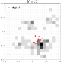
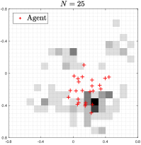
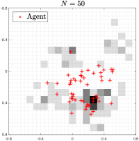
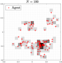
Figure 2: The figure shows the steady state distribution of the agents implementing the coverage algorithm (20) with the target distribution depicted in grayscale, for $N=10,25,50,100$. We observe that the distribution of the agents more closely approximates the target distribution as the size $N$ of the system increases.

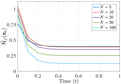
Figure 3: The figure is a representative plot of the value of the aggregate objective function $\bar{\mathcal{H}}_{f}(\mathbf{x}_{t})$ (with $f(x)=x^{2}$) vs. time $t$ for various sizes $N$ of the multi-agent system and random initializations of agent positions. We observe that the steady state value decreases with the size $N$ of the system, in accordance with our theoretical results.

7 Conclusion

In this paper, we have introduced a multiscale framework for the analysis and design of multi-agent coverage algorithms that begins with a macroscopic specification of the target coverage behavior to derive provably-correct microscopic, agent-level algorithms that achieve the target macroscopic specification. Our class of macroscopic proximal descent schemes exploit convexity properties of coverage objective functionals to steer the macroscopic configuration, which are then translated into agent-level algorithms via a variational discretization. We uncover the relationship with previously studied coverage algorithms, and obtain insights into the large-scale behavior of these algorithms. Future work will consider the extension to a constrained optimization framework to include such constraints as sensing limitations, dynamic and collision-avoidance constraints. We have assumed in this paper that the underlying spatial domain $\Omega$ is convex. This assumption results in the convexity of the space of probability measures. The convexity of the space of probability measures (which is the search space in our proximal descent schemes) is necessary for the minimization problems we obtain to be convex. The presence of obstacles in the mission space is likely to violate this assumption and lead to non-convexity of the corresponding minimization problems. Overcoming this difficulty is a consideration for future work.

Appendix A Additional preliminaries

We present here the mathematical preliminaries on convergence of measures, the $L^{2}$-Wasserstein space and smoothness and convexity notions for functions defined on the $L^{2}$-Wasserstein space.

A.1 Convexity of functions

Recall that a set $\Omega\subseteq^{d}$ is convex if for $x,y\in\Omega$, we have $(1-t)x+ty\in\Omega$ for all $t\in[0,1]$. A function $f:\Omega\rightarrow$ is convex if $\Omega$ is convex and $f((1-t)x+ty)\leq(1-t)f(x)+tf(y)$ for all $t\in[0,1]$. A function $f:\Omega\rightarrow$ is $m$-strongly convex if $\Omega$ is convex and $f((1-t)x+ty)\leq(1-t)f(x)+tf(y)-\frac{1}{2}mt(1-t)\|x-y\|^{2}$ for all $t\in[0,1]$ and some $m>0$.

A.2 The space of probability measures and its topology

Let $\Omega=\bar{D}$, with $D\subset^{d}$ an open, bounded set in the $d$-dimensional Euclidean space ^d. Let $\mathcal{B}(\Omega)$ be the Borel $\sigma$-algebra in $\Omega$, which is the collection of measurable sets w.r.t. Borel measures. The space of probability measures, $\mathcal{P}(\Omega)$, is the collection of functions $\mu:\mathcal{B}(\Omega)\rightarrow[0,1]$ satisfying the following properties: (a) $\mu\left(\emptyset\right)=0$, (b) $\mu\left(\Omega\right)=1$, and (c) (sub-additivity) $\mu\left(\cup_{i\in\mathbb{N}}A_{i}\right)=\sum_{i}\mu(A_{i})$, for a countable family of pairwise disjoint sets $\{A_{i}\,|\,A_{i}\in\mathcal{B}(\Omega)\}$. We denote by $\mathcal{P}^{r}(\Omega)\subset\mathcal{P}(\Omega)$ the space of atomless probability measures, where a measure $\mu\in\mathcal{P}(\Omega)$ is said to be atomless if for any $A\in\mathcal{B}(\Omega)$ with $\mu(A)>0$, there exists $B\in\mathcal{B}(\Omega)$, $B\subset A$, such that $\mu(A)>\mu(B)>0$. It follows that for an atomless measure $\mu$, we will have $\mu(\{x\})=0$ for all $x\in\Omega$. We consider this a notion of regularity of probability measures, and hence the use of the superscript $r$ in $\mathcal{P}^{r}(\Omega)$. We refer to [7] for other basic definitions in measure theory. Finally, we recall the following:

Definition 6 (Pushforward measure).

Let $\Omega,\Theta$ be (Borel) measurable spaces, a measurable mapping $\mathcal{T}:\Omega\rightarrow\Theta$ and consider a measure $\mu\in\mathcal{P}(\Omega)$. The pushforward measure $\nu=\mathcal{T}_{\#}\mu\in\mathcal{P}(\Theta)$ of $\mu$ is defined as $\nu(B)=\mathcal{T}_{\#}\mu(B)=\mu(\mathcal{T}^{-1}(B))$, for all Borel measurable $B\subseteq\Theta$.

A.3 Weak convergence of measures

The results of this manuscript rely on the notions of weak convergence in $\mathcal{P}(\Omega)$, the topology of weak convergence, its metrizability, and the compactness of sets of $\mathcal{P}(\Omega)$. We recall them here and refer the reader to [7] for more information.

Definition 7 (Weak convergence).

Let $\Omega\subseteq^{d}$, and $\mathcal{P}(\Omega)$ be its set of probability measures. A sequence $\{\mu_{k}\}_{k\in\mathbb{N}}\subseteq\mathcal{P}(\Omega)$ converges weakly to $\mu\in\mathcal{P}(\Omega)$ if for any bounded and continuous function $f$ on $\Omega$, $\lim_{k\rightarrow\infty}\int_{\Omega}fd\mu_{k}=\int_{\Omega}fd\mu$.

Equivalently, in the definition above, the sequence $\{\mu_{k}\}_{k\in\mathbb{N}}$ in $\mathcal{P}(\Omega)$ is said to converge to $\mu$ in $\mathcal{P}(\Omega)$ equipped with the topology of weak convergence. The space of probability measures $\mathcal{P}(\Omega)$ equipped with the topology of weak convergence is metrizable [7]. In other words, there exists a metric on $\mathcal{P}(\Omega)$ such that the topology of weak convergence is obtained as the topology induced by the metric. One such metric is the Wasserstein distance, see Section A.4. We now state Prokhorov’s theorem [7] on the equivalence between tightness and precompactness of a collection of probability measures over a separable and complete metric (Polish) space.

Lemma 12 (Prokhorov’s theorem).

Let $\Omega$ be a complete metric space, and let $\mathcal{K}\subseteq\mathcal{P}(\Omega)$. The closure of $\mathcal{K}$ w.r.t. the topology of weak convergence in $\mathcal{P}(\Omega)$ is compact if and only if $\mathcal{K}$ is tight. That is, $\mathcal{K}$ is tight if for any $\epsilon>0$ there exists a compact $K_{\epsilon}\subseteq\Omega$ such that $\mu(K_{\epsilon})>1-\epsilon$, for all $\mu\in\mathcal{K}$.

Corollary 3 (Compactness of $\mathcal{P}(\Omega)$).

Let $\Omega\subseteq^{d}$ a compact set. Then, the closure of $\mathcal{P}(\Omega)$ w.r.t. the topology of weak convergence in $\mathcal{P}(\Omega)$ is compact. This follows from Prokhorov’s theorem in Lemma 12, since $\mathcal{P}(\Omega)$ is tight: for any $\epsilon>0$, we choose $\Omega$ itself as the compact set and have $\mu(\Omega)=1>1-\epsilon$ for any $\mu\in\mathcal{P}(\Omega)$. Moreover, since $\mathcal{P}(\Omega)$ is also closed w.r.t. the topology of weak convergence, it is therefore compact.

A.4 The $L^{2}$-Wasserstein distance

The $L^{2}$-Wasserstein distance between two probability measures $\mu,\nu\in\mathcal{P}(\Omega)$ is given by:

$$W_{2}^{2}(\mu,\nu)=\min_{\pi\in\Pi(\mu,\nu)}\int_{\Omega\times\Omega}|x-y|^{2}~{}d\pi(x,y),$$ (22)

where $\Pi(\mu,\nu)$ is the space of joint probability measures over $\Omega\times\Omega$ with marginals $\mu$ and $\nu$. The definition of $L^{2}$-Wasserstein distance in (22) follows from the so-called Kantorovich formulation of optimal transport. An alternative formulation of this problem, called the Monge formulation of optimal transport, is given below:

$$W_{2}^{2}(\mu,\nu)=\min_{\begin{subarray}{c}T:\Omega\rightarrow\Omega\\ T_{\#}\mu=\nu\end{subarray}}\int_{\Omega}|x-T(x)|^{2}~{}d\mu(x).$$ (23)

In the Monge formulation (23), the minimization is carried out over the space of maps $T:\Omega\rightarrow\Omega$ for which the probability measure $\nu$ is obtained as the pushforward of $\mu$. This can be viewed as a deterministic formulation of optimal transport, where the transport is carried out by a map, whereas the Kantorovich formulation (22) can be seen as a problem relaxation, where the transport plan is described by a joint probability measure $\pi$ over $\Omega\times\Omega$, with $\mu$ and $\nu$ as its marginals. It is to be noted that the Monge formulation does not always admit a solution, while the Kantorovich problem does. Roughly speaking, the Kantorovich formulation is the “minimal” extension of the Monge formulation, as both problems attain the same infimum [46]. Further, the two formulations (22) and (23) are equivalent under certain conditions [46]. The space of probability measures $\mathcal{P}(\Omega)$ endowed with the $L^{2}$-Wasserstein distance $W_{2}$ will equivalently be referred to as the $L^{2}$-Wasserstein space $(\mathcal{P}(\Omega),W_{2})$ over $\Omega$. The following lemma, which follows from Theorem 6.9 in [50], establishes the equivalence between convergence in the sense of the topology of weak convergence and in the $L^{2}$-Wasserstein metric.

Lemma 13 (Convergence in $(\mathcal{P}(\Omega),W_{2})$).

For compact $\Omega\subset^{d}$, the $L^{2}$-Wasserstein distance $W_{2}$ metrizes the weak convergence in $\mathcal{P}(\Omega)$. That is, a sequence of measures $\{\mu_{k}\}_{k\in\mathbb{N}}$ in $\mathcal{P}(\Omega)$ converges weakly to $\mu\in\mathcal{P}(\Omega)$ if and only if $\lim_{k\rightarrow\infty}W_{2}(\mu_{k},\mu)=0$.

Appendix B Fréchet differentials of functionals on atomless measures

Let $\mu_{0},\mu_{1}\in\mathcal{P}^{\rm a}(\Omega)$ be atomless probability measures, and let $T_{\mu_{0}\rightarrow\mu_{1}}$ be the optimal transport map from $\mu_{0}$ to $\mu_{1}$. Furthermore, for $\epsilon\in[0,1]$, let:

$$\mu_{\epsilon}=((1-\epsilon)\operatorname{id}+\epsilon T_{\mu_{0}\rightarrow\mu_{1}})_{\#}\mu_{0}.$$ (24)

We now begin by introducing the notion of first variation of a functional on $\mathcal{P}(\Omega)$ as follows:

Definition 8 (First variation of a functional on $\mathcal{P}(\Omega)$).

Let $F:\mathcal{P}(\Omega)\rightarrow$ and $\mu_{0}\in\mathcal{P}^{\rm a}(\Omega)$. Suppose that there exists a unique $\varphi$ such that for any $\mu_{1}\in\mathcal{P}^{\rm a}(\Omega)$ and $\{\mu_{\epsilon}\}_{\epsilon\in[0,1]}$ as defined in (24), the following holds:

$$\left.\frac{d}{d\epsilon}F(\mu_{\epsilon})\right|_{\epsilon=0}=\lim_{\epsilon\rightarrow 0^{+}}\frac{1}{\epsilon}\int_{\Omega}\varphi\left(d\mu_{\epsilon}-d\mu_{0}\right).$$

Then $\varphi$ is the first variation of $F$ evaluated at $\mu_{0}$, denoted as $\varphi=\frac{\delta F}{\delta\mu}(\mu_{0})$.

For functionals for which the first variation exists as in the above definition, we can introduce the notion of Fréchet derivative on the $L^{2}$-Wasserstein space $(\mathcal{P}(\Omega),W_{2})$:

Definition 9 (Derivative of a functional on $(\mathcal{P}(\Omega),W_{2})$).

A functional $F:\mathcal{P}(\Omega)\rightarrow$ is Fréchet differentiable with derivative $\xi\in L^{2}((\Omega,\mu);^{d})$ at an atomless measure $\mu_{0}\in\mathcal{P}^{\rm a}(\Omega)$ if for any $\mu_{1}\in\mathcal{P}^{\rm a}(\Omega)$ and $\{\mu_{\epsilon}\}_{\epsilon\in[0,1]}$ as defined in (24), the following holds:

$$\lim_{\epsilon\rightarrow 0^{+}}\frac{F(\mu_{\epsilon})-F(\mu_{0})-\int_{\Omega}\left\langle\xi,T_{\mu_{0}\rightarrow\mu_{\epsilon}}-\operatorname{id}\right\rangle d\mu_{0}}{W_{2}(\mu_{0},\mu_{1})}=0,$$

where $\xi=\nabla\varphi$ and $\varphi=\frac{\delta F}{\delta\tilde{\mu}}(\mu_{0})$.

Furthermore, we define the directional derivative of $F$ at $\mu_{0}$ along a tangent vector field $\mathbf{v}\in L^{2}((\Omega,\mu);^{d})$ as:

$$D_{\mathbf{v}}F(\mu_{0})=\int_{\Omega}\left\langle\xi,\mathbf{v}\right\rangle d\mu,$$

where $\xi$ is the Fréchet derivative of $F$ evaluated at $\mu_{0}$.

Appendix C Results on regularity of functionals

The following lemma can be verfied for strongly geodesically convex functionals as in Definition 3:

Lemma 14 (Strongly geodesically convex functionals).

Let $F:\mathcal{P}(\Omega)\rightarrow$ be an $m$-strongly (generalized) geodesically convex functional on $(\mathcal{P}(\Omega),W_{2})$ w.r.t base measure $\theta\in\mathcal{P}^{\rm a}(\Omega)$. Let $\mu,\nu\in\mathcal{P}^{\rm a}(\Omega)$ be atomless probability measures and let $\xi_{\mu}$, $\xi_{\nu}$ and $\xi_{\theta}$ be the Fréchet derivatives of $F$ evaluated at $\mu$, $\nu$ and $\theta$ respectively. The following holds:

$$\int_{\Omega}\left\langle\xi_{\nu}(T_{\theta\rightarrow\nu})-\xi_{\mu}(T_{\theta\rightarrow\mu}),T_{\theta\rightarrow\nu}-T_{\theta\rightarrow\mu}\right\rangle d\theta$$

$$\geq m\int_{\Omega}\left|T_{\theta\rightarrow\nu}-T_{\theta\rightarrow\mu}\right|^{2}d\theta,$$

where $T_{\theta\rightarrow\mu}:\Omega\rightarrow\Omega$ and $T_{\theta\rightarrow\nu}:\Omega\rightarrow\Omega$ are optimal transport maps from $\theta$ to $\mu$ and from $\theta$ to $\nu$ respectively.

Similarly, the following lemma can be verfied for $l$-smooth functionals as defined in 4:

Lemma 15 ($l$-smooth functionals).

Let $F:\mathcal{P}(\Omega)\rightarrow$ be an $l$-smooth functional on $(\mathcal{P}(\Omega),W_{2})$ w.r.t. a base measure $\theta\in\mathcal{P}^{\rm a}(\Omega)$. Let $\mu,\nu\in\mathcal{P}^{\rm a}(\Omega)$ be atomless probability measures and let $\xi_{\mu}$, $\xi_{\nu}$ and $\xi_{\theta}$ be the Fréchet derivatives of $F$ evaluated at $\mu$, $\nu$ and $\theta$ respectively. The following holds:

$$\left|\int_{\Omega}\left\langle\xi_{\nu}(T_{\theta\rightarrow\nu})-\xi_{\mu}(T_{\theta\rightarrow\mu}),T_{\theta\rightarrow\nu}-T_{\theta\rightarrow\mu}\right\rangle d\theta\right|$$

$$\leq l\int_{\Omega}\left|T_{\theta\rightarrow\nu}-T_{\theta\rightarrow\mu}\right|^{2}d\theta.$$

Appendix D Supporting results for Theorem 1

Lemma 16 (Compactness and convexity of sublevel sets).

Let $F$ satisfy the regularity conditions of Assumption 1. Then, the $F$-sublevel set of any absolutely continuous probability measure $\mu\in\mathcal{P}(\Omega)$ is compact and geodesically convex in the $L^{2}$-Wasserstein space $(\mathcal{P}(\Omega),W_{2})$.

Proof.

For any $\mu\in\mathcal{P}(\Omega)$, the sublevel set $\mathcal{S}({\mu})=\{\nu\in\mathcal{P}(\Omega)|F(\nu)\leq F(\mu)\}$ is closed in $(\mathcal{P}(\Omega),W_{2})$, since $F$ is continuous and $\mathcal{P}(\Omega)$ is closed and compact. This implies that $\mathcal{S}({\mu})$ is also compact since it is a closed subset of a compact set.

It holds that $(\mathcal{P}(\Omega),W_{2})$ is geodesically convex, and consider, for any $\nu_{0},\nu_{1}\in\mathcal{S}({\mu})$, and $\nu_{t}\in\mathcal{P}(\Omega)$, for $t\in[0,1]$, the generalized geodesic between $\nu_{0}$ to $\nu_{1}$ with $\mu$ as the reference measure. From the (generalized) geodesic convexity of $F$ we have that $F(\nu_{t})\leq(1-t)F(\nu_{0})+tF(\nu_{1})\leq F(\mu)$ (since $F(\nu_{0})\leq F(\mu)$ and $F(\nu_{1})\leq F(\mu)$ by definition of $\mathcal{S}({\mu})$). This implies that $\nu_{t}\in\mathcal{S}({\mu})$ for any $t\in[0,1]$, from which we infer the geodesic convexity of $\mathcal{S}({\mu})$.

∎

Lemma 17 (Strong convexity of objective functional).

Let $F$ satisfy the regularity conditions of Assumption 1. For any absolutely continuous probability measure $\mu\in\mathcal{P}(\Omega)$, the functional $G(\nu)=\frac{1}{2\tau}W_{2}^{2}(\mu,\nu)+F(\nu)$ is $\left(\frac{1}{\tau}-l\right)$-strongly (generalized) geodesically convex (in the sense of Definition 3 w.r.t. reference measure $\mu$) over $\mathcal{P}^{\textup{a}}(\Omega)$ for $0<\tau<1/l$.

Proof.

Since $F$ is $l$-smooth w.r.t. any (atomless) base measure, applying Lemma 15 for two atomless measures $\nu_{1}$ and $\nu_{2}$, we get:

$$\begin{aligned} &\left|\int_{\Omega}\left\langle\xi_{2}(T_{\mu\rightarrow\nu_{2}})-\xi_{1}(T_{\mu\rightarrow\nu_{1}}),T_{\mu\rightarrow\nu_{2}}-T_{\mu\rightarrow\nu_{1}}\right\rangle d\mu\right|\\ &\leq l\int_{\Omega}\left|T_{\mu\rightarrow\nu_{2}}-T_{\mu\rightarrow\nu_{1}}\right|^{2}d\mu,\end{aligned}$$ (25)

where $\xi_{1}$ and $\xi_{2}$ are the Fréchet derivatives of $F$ evaluated at $\nu_{1}$ and $\nu_{2}$, respectively, and $T_{\mu\rightarrow\nu_{1}}$ and $T_{\mu\rightarrow\nu_{2}}$ are the optimal transport maps from $\mu$ to $\nu_{1}$ and $\nu_{2}$, respectively. Let $\eta_{i}=\left.\nabla\left(\frac{\delta G}{\delta\nu}\right)\right|_{\nu_{i}}$, for $i=1,2$, and let $\phi_{i}=\frac{1}{2}\left.\frac{\delta W_{2}^{2}(\mu,\nu)}{\delta\nu}\right|_{\nu_{i}}$ be the so-called Kantorovich potential for the transport from $\nu_{1}$ to $\mu$, for $i=1,2$. We now have:

$$\int_{\Omega}\left\langle\eta_{2}(T_{\mu\rightarrow\nu_{2}})-\eta_{1}(T_{\mu\rightarrow\nu_{1}}),T_{\mu\rightarrow\nu_{2}}-T_{\mu\rightarrow\nu_{1}}\right\rangle d\mu$$

$$=\int_{\Omega}\left\langle\frac{1}{\tau}\nabla\phi_{2}(T_{\mu\rightarrow\nu_{2}})-\frac{1}{\tau}\nabla\phi_{1}(T_{\mu\rightarrow\nu_{1}})\right.$$

$$\qquad\left.-\xi_{1}(T_{\mu\rightarrow\nu_{1}})+\xi_{2}(T_{\mu\rightarrow\nu_{2}}),T_{\mu\rightarrow\nu_{2}}-T_{\mu\rightarrow\nu_{1}}\right\rangle d\mu$$

$$=\frac{1}{\tau}\int_{\Omega}\left\langle\nabla\phi_{2}(T_{\mu\rightarrow\nu_{2}})-\nabla\phi_{1}(T_{\mu\rightarrow\nu_{1}}),T_{\mu\rightarrow\nu_{2}}-T_{\mu\rightarrow\nu_{1}}\right\rangle d\mu$$

$$\qquad+\int_{\Omega}\left\langle\xi_{2}(T_{\mu\rightarrow\nu_{2}})-\xi_{1}(T_{\mu\rightarrow\nu_{1}}),T_{\mu\rightarrow\nu_{2}}-T_{\mu\rightarrow\nu_{1}}\right\rangle d\mu$$

$$\geq\left(\frac{1}{\tau}-l\right)\int_{\Omega}\left|T_{\mu\rightarrow\nu_{2}}-T_{\mu\rightarrow\nu_{1}}\right|^{2}d\mu,$$

where the penultimate inequality above follows from (25).

We have also used the fact that $\int_{\Omega}\left\langle\nabla\phi_{2}(T_{\mu\rightarrow\nu_{2}})-\nabla\phi_{1}(T_{\mu\rightarrow\nu_{1}}),T_{\mu\rightarrow\nu_{2}}-T_{\mu\rightarrow\nu_{1}}\right\rangle d\mu=\int_{\Omega}\left|T_{\mu\rightarrow\nu_{2}}-T_{\mu\rightarrow\nu_{1}}\right|^{2}d\mu$ (this follows from an application of [46, Theorem 1.17]). Since $\tau<\frac{1}{l}$, we get that the functional $G$ is strongly convex with parameter $\frac{1}{\tau}-l$.

∎

Appendix E Proof of Proposition 1

Let $\widehat{\mu}^{N}_{\mathbf{x},\mathbf{w}}=\sum_{i=1}^{N}w_{i}\delta_{x_{i}}$ be a weighted discrete probability measure corresponding to $\left\{x_{i}\right\}_{i=1}^{N}$ with weights $\{w_{i}\}_{i=1}^{N}$, such that $w_{i}\in[0,1]$ and $\sum_{i=1}^{N}w_{i}=1$. The optimal transport cost between $\widehat{\mu}^{N}_{\mathbf{x},\mathbf{w}}$ and $\mu^{\star}$ is given by:

$$C_{f}(\widehat{\mu}^{N}_{\mathbf{x},\mathbf{w}},\mu^{\star})=\inf_{\begin{subarray}{c}T:\Omega\rightarrow\Omega\\ T_{\#}\mu^{\star}=\widehat{\mu}^{N}_{\mathbf{x}}\end{subarray}}~{}\int_{\Omega}f(|x-T(x)|)~{}d\mu^{\star}(x),$$

where the infimum is over the set of maps $T$ that pushforward $\mu^{\star}$ to $\widehat{\mu}^{N}_{\mathbf{x},\mathbf{w}}$ (since $\widehat{\mu}^{N}_{\mathbf{x},\mathbf{w}}$ has finite support, pushforward maps exist only from $\mu^{\star}$ to $\widehat{\mu}^{N}_{\mathbf{x},\mathbf{w}}$ and not the other way around). Transport maps $T:\Omega\rightarrow\{x_{i}\}_{i=1}^{N}$ partition $\Omega$ into $N$ regions $\left\{\mathcal{W}_{i}\right\}_{i=1}^{N}$, where $\mathcal{W}_{i}=\{x\in\Omega\,|\,T(x)=x_{i}\}$, of mass $\mu^{\star}(\mathcal{W}_{i})=w_{i}$. Let $T^{\star}:\Omega\rightarrow\{x_{i}\}_{i=1}^{N}$ be the optimal transport map from $\mu^{\star}$ to $\widehat{\mu}^{N}_{\mathbf{x},\mathbf{w}}$, which allows us to write:

$$C_{f}(\widehat{\mu}^{N}_{\mathbf{x},\mathbf{w}},\mu^{\star})=\inf_{\begin{subarray}{c}T:\Omega\rightarrow\Omega\\ T_{\#}\mu^{\star}=\widehat{\mu}^{N}_{\mathbf{x},\mathbf{w}}\end{subarray}}~{}\int_{\Omega}f(|x-T(x)|)~{}d\mu^{\star}(x)$$

$$=\int_{\Omega}f(|x-T^{\star}(x)|)~{}d\mu^{\star}(x)=\sum_{i=1}^{N}\int_{\mathcal{W}_{i}^{\star}}f(|x-x_{i}|)~{}d\mu^{\star}(x)$$

$$\qquad\geq\sum_{i=1}^{N}\int_{\mathcal{V}_{i}}f(|x-x_{i}|)~{}d\mu^{\star}(x).$$ (26)

The above inequality, which holds for any choice of $\mathbf{w}$, follows from the fact that $f$ is non-decreasing, and the definition of the Voronoi partition $\{\mathcal{V}_{i}\}_{i=1}^{N}$. As $f$ is non-decreasing:

$$\int_{\Omega}\min_{i\in\{1,\ldots,N\}}f(|x-x_{i}|)d\mu^{\star}(x)=\sum_{i=1}^{N}\int_{\mathcal{V}_{i}}f(|x-x_{i}|)d\mu^{\star}(x),$$

where $\{\mathcal{V}_{i}\}_{i=1}^{N}$ is the Voronoi partition of $\Omega$. We now define a map $T_{\mathcal{V}}:\Omega\rightarrow\Omega$ such that $T_{\mathcal{V}}(x)=x_{i}$ for $x\in\mathcal{V}_{i}$, with $T_{\mathcal{V}}(\Omega)=\{x_{1},\ldots,x_{N}\}$, for which the following holds:

$$\int_{\Omega} f(|x-T_{\mathcal{V}}(x)|)~{}d\mu^{\star}(x)=\sum_{i=1}^{N}\int_{\mathcal{V}_{i}}f(|x-x_{i}|)~{}d\mu^{\star}(x)$$

$$=\int_{\Omega}\min_{i\in\{1,\ldots,N\}}f(|x-x_{i}|)~{}d\mu^{\star}(x).$$

From (26) and the above, we therefore get:

$$\int_{\Omega}f(|x-T_{\mathcal{V}}(x)|)~{}d\mu^{\star}(x)\leq C_{f}(\widehat{\mu}^{N}_{\mathbf{x},\mathbf{w}},\mu^{\star}).$$

For the particular choice of the weights $w_{i}^{\star}=\mu^{\star}(\mathcal{V}_{i})$, such that $\widehat{\mu}^{N}_{\mathbf{x},\mu^{\star}(\mathcal{V})}=\sum_{i=1}^{N}\mu^{\star}(\mathcal{V}_{i})\delta_{x_{i}}$, we also get the inequality:

$$C_{f}\left(\sum_{i=1}^{N}\mu^{\star}(\mathcal{V}_{i})\delta_{x_{i}},\mu^{\star}\right)$$

$$=\inf_{\begin{subarray}{c}T:\Omega\rightarrow\Omega\\ T_{\#}\mu^{\star}=\sum_{i=1}^{N}\mu^{\star}(\mathcal{V}_{i})\delta_{x_{i}}\end{subarray}}~{}\int_{\Omega}f(|x-T(x)|)~{}d\mu^{\star}(x)$$

$$\leq\int_{\Omega}f(|x-T_{\mathcal{V}}(x)|)~{}d\mu^{\star}(x),$$

and we therefore get:

$$C_{f}\left(\sum_{i=1}^{N}\mu^{\star}(\mathcal{V}_{i})\delta_{x_{i}},\mu^{\star}\right)=\int_{\Omega}\min_{i\in\{1,\ldots,N\}}f(|x-x_{i}|)~{}d\mu^{\star}(x),$$

which establishes that:

$$\min_{\begin{subarray}{c}\mathbf{w}\in{\mathbb{R}}_{\geq 0}^{N}\end{subarray}}C_{f}\left(\sum_{i=1}^{N}w_{i}\delta_{x_{i}},\mu^{\star}\right) =\int_{\Omega}\min_{i\in\{1,\ldots,N\}}f(|x-x_{i}|)~{}d\mu^{\star}(x)$$

$$=\mathcal{H}_{f}(\mathbf{x}),$$

with the minimizing weights $w_{i}^{\star}=\mu^{\star}(\mathcal{V}_{i})$.

Appendix F Aggregate objective functions

Proposition 2 (Strict geodesic convexity of $C_{f}(\cdot,\mu^{*})$).

Fix $\mu^{*}\in\mathcal{P}(\Omega)$ (absolutely continuous) as the reference measure and let $\mu_{0},\mu_{1}\in\mathcal{P}(\Omega)$. Let $T_{\mu^{*}\rightarrow\mu_{0}}$ and $T_{\mu^{*}\rightarrow\mu_{1}}$ be optimal transport maps from $\mu^{*}$ to $\mu_{0}$ and $\mu^{*}$ to $\mu_{1}$ respectively, corresponding to the optimal transport cost $C_{f}$, and let $T_{t}=(1-t)T_{\mu^{*}\rightarrow\mu_{0}}+tT_{\mu^{*}\rightarrow\mu_{1}}$ for $t\in[0,1]$. For $\mu_{t}={T_{t}}_{\#}\mu^{*}$, we have:

$$C_{f}(\mu_{t},\mu^{*})<(1-t)C_{f}(\mu_{0},\mu^{*})+tC_{f}(\mu_{1},\mu^{*}).$$

Proof.

We have:

$$C_{f}(\mu_{t},\mu^{*})\leq\int_{\Omega}f(|T_{t}(x)-x|)d\mu^{*}(x)$$

$$=\int_{\Omega}f\left(\left|(1-t)T_{\mu^{*}\rightarrow\mu_{0}}(x)+tT_{\mu^{*}\rightarrow\mu_{1}}(x)-x\right|\right)d\mu^{*}(x)$$

$$=\int_{\Omega}f\left(\left|(1-t)\left[T_{\mu^{*}\rightarrow\mu_{0}}(x)-x\right]\right.\right.$$

$$\left.\left.\qquad\qquad+t\left[T_{\mu^{*}\rightarrow\mu_{1}}(x)-x\right]\right|\right)d\mu^{*}(x)$$

$$\leq\int_{\Omega}f\left((1-t)\left|T_{\mu^{*}\rightarrow\mu_{0}}(x)-x\right|\right.$$

$$\left.\qquad\qquad+t\left|T_{\mu^{*}\rightarrow\mu_{1}}(x)-x\right|\right)d\mu^{*}(x),$$

where the last inequality is a consequence of the fact that $f$ is non-decreasing. Further, if $f$ is strictly convex in $\Omega$, we have:

$$C_{f}(\mu_{t},\mu^{*})$$

$$<\int_{\Omega}\left[(1-t)f\left(\left|T_{\mu^{*}\rightarrow\mu_{0}}(x)-x\right|\right)\right.$$

$$\left.\qquad\qquad+tf\left(\left|T_{\mu^{*}\rightarrow\mu_{1}}(x)-x\right|\right)\right]d\mu^{*}(x)$$

$$=(1-t)\int_{\Omega}f\left(\left|T_{\mu^{*}\rightarrow\mu_{0}}(x)-x\right|\right)d\mu^{*}(x)$$

$$\qquad\qquad+t\int_{\Omega}f\left(\left|T_{\mu^{*}\rightarrow\mu_{1}}(x)-x\right|\right)d\mu^{*}(x)$$

$$=(1-t)C_{f}(\mu_{0},\mu^{*})+tC_{f}(\mu_{1},\mu^{*}).$$

$\square$∎

We now establish the following result:

Proposition 3 ($l$-smoothness of $C_{f}(\cdot,\mu^{*})$).

Let the Fréchet derivative of the functional $F(\mu)=C_{f}(\mu,\mu^{*})$ at $\mu\in\mathcal{P}^{r}(\Omega)$ be denoted as $\xi_{\mu}$. The derivative $\xi_{\mu}$ satisfies:

$$\left|\int_{\Omega}\left\langle\xi_{\mu_{2}}(T_{\mu^{*}\rightarrow\mu_{2}})-\xi_{\mu_{1}}(T_{\mu^{*}\rightarrow\mu_{1}}),T_{\mu^{*}\rightarrow\mu_{2}}-T_{\mu^{*}\rightarrow\mu_{1}}\right\rangle d\mu^{*}\right|$$

$$\leq l\int_{\Omega}\left|T_{\mu^{*}\rightarrow\mu_{2}}-T_{\mu^{*}\rightarrow\mu_{1}}\right|^{2}d\mu^{*},$$

where $T_{\mu^{*}\rightarrow\mu_{1}}$ and $T_{\mu^{*}\rightarrow\mu_{2}}$ are the optimal transport maps (w.r.t. $f$) from $\mu^{*}$ to $\mu_{1}$ and $\mu_{2}$, respectively.

Proof.

Let $\phi_{\mu}=\frac{\delta C_{f}(\mu,\mu^{*})}{\delta\mu}$ be the Kantorovich potential for the optimal transport from $\mu$ to $\mu^{*}$. We now have the following relation [46, Theorem 1.17]:

$$T_{\mu\rightarrow\mu^{*}}=\operatorname{id}-\left(\nabla h\right)^{-1}(\nabla\phi_{\mu}),$$

where the function $h:^{d}\rightarrow$ is such that $h(\mathbf{v})=f(|\mathbf{v}|)$. It follows from the $l$-smoothness of $f$ that the function $h$ is also $l$-smooth. From the above and $l$-smoothness of $h$, (with $\xi_{\mu}=\nabla\phi_{\mu}$) we get:

$$\left|\int_{\Omega}\left\langle\xi_{\mu_{2}}(T_{\mu^{*}\rightarrow\mu_{2}})-\xi_{\mu_{1}}(T_{\mu^{*}\rightarrow\mu_{1}}),T_{\mu^{*}\rightarrow\mu_{2}}-T_{\mu^{*}\rightarrow\mu_{1}}\right\rangle d\mu^{*}\right|$$

$$=\left|\int_{\Omega}\left\langle\nabla h\left(T_{\mu^{*}\rightarrow\mu_{2}}-\operatorname{id}\right)\right.\right.$$

$$\qquad\qquad\left.\left.-\nabla h\left(T_{\mu^{*}\rightarrow\mu_{1}}-\operatorname{id}\right),T_{\mu^{*}\rightarrow\mu_{2}}-T_{\mu^{*}\rightarrow\mu_{1}}\right\rangle d\mu^{*}\right|$$

$$\leq\int_{\Omega}\left|\left\langle\nabla h\left(T_{\mu^{*}\rightarrow\mu_{2}}-\operatorname{id}\right)\right.\right.$$

$$\qquad\qquad\left.\left.-\nabla h\left(T_{\mu^{*}\rightarrow\mu_{1}}-\operatorname{id}\right),T_{\mu^{*}\rightarrow\mu_{2}}-T_{\mu^{*}\rightarrow\mu_{1}}\right\rangle\right|d\mu^{*}$$

$$\leq l\int_{\Omega}\left|T_{\mu^{*}\rightarrow\mu_{2}}-T_{\mu^{*}\rightarrow\mu_{1}}\right|^{2}d\mu^{*}.$$

$\square$∎

Proposition 4 (Lipschitz continuous Fréchet derivative of $C_{f}(\cdot,\mu^{*})$).

Let the Fréchet derivative of the functional $F(\mu)=C_{f}(\mu,\mu^{*})$ at $\mu\in\mathcal{P}^{r}(\Omega)$ be denoted as $\xi_{\mu}$. For any $x,x^{\prime}\in\Omega$, the derivative $\xi_{\mu}$ satisfies:

$$\left\|\xi_{\mu}(x)-\xi_{\mu}(x^{\prime})\right\|\leq\lambda\left\|x-x^{\prime}\right\|.$$

Proof.

From Proposition 3, we note that $\xi_{\mu}=\nabla h\left(\operatorname{id}-T_{\mu\rightarrow\mu^{*}}\right)$ on $\Omega$, where $\nabla h$ is Lipschitz continuous (with constant $l$). Therefore, for any $x,x^{\prime}\in\Omega$ we have:

$$\left\|\xi_{\mu}(x)-\xi_{\mu}(x^{\prime})\right\|$$

$$=\left\|\nabla h\left(x-T_{\mu\rightarrow\mu^{*}}(x)\right)-\nabla h\left(x^{\prime}-T_{\mu\rightarrow\mu^{*}}(x^{\prime})\right)\right\|$$

$$\leq l\left\|x-x^{\prime}\right\|+l\left\|T_{\mu\rightarrow\mu^{*}}(x)-T_{\mu\rightarrow\mu^{*}}(x^{\prime})\right\|$$

$$\leq\underbrace{l\left(1+\operatorname{lip}(T_{\mu\rightarrow\mu^{*}})\right)}_{\lambda}\left\|x-x^{\prime}\right\|,$$

where the final inequality follows from the fact that $T_{\mu\rightarrow\mu^{*}}$ is a Lipschitz continuous map on $\Omega$ (with Lipschitz constant $\operatorname{lip}(T_{\mu\rightarrow\mu^{*}})$) [46, Chapter 1.3]. ∎

Appendix G Proofs of Lemmas

G.1 Proof of Lemma 2

We first recall that $F^{h,N}(\mathbf{x})=F(\widehat{\mu}^{h,N}_{\mathbf{x}})$. By the Glivenko-Cantelli Theorem [49] and Assumption 3-(iv), we have:

$$\lim_{\begin{subarray}{c}h\rightarrow 0,\\ N\rightarrow\infty\end{subarray}}\sup_{f\in\mathcal{M}}\left\{\mathbb{E}_{\widehat{\mu}^{h,N}_{\mathbf{x}}}[f]-\mathbb{E}_{\mu}[f]\right\}=0,~{}~{}a.s.$$

We denote the above as $\widehat{\mu}^{h,N}_{\mathbf{x}}\rightarrow_{\mathrm{u.a.s}}~{}\mu$, i.e., $\widehat{\mu}^{h,N}_{\mathbf{x}}$ converges uniformly almost surely to $\mu$ as $h\rightarrow 0$ and $N\rightarrow\infty$. Note that this implies the (almost sure) weak convergence of $\{\widehat{\mu}^{h,N}_{\mathbf{x}}\}$ to $\mu$. Therefore, by continuity of $F$ in the topology of weak convergence (which follows from the fact that $F$ is Frećhet differentiable in the $L^{2}$-Wasserstein space), we have $\lim_{\begin{subarray}{c}h\rightarrow 0,N\rightarrow\infty\end{subarray}}F^{h,N}(\mathbf{x})=\lim_{\begin{subarray}{c}h\rightarrow 0,N\rightarrow\infty\end{subarray}}F(\widehat{\mu}^{h,N}_{\mathbf{x}})=F(\lim_{\begin{subarray}{c}h\rightarrow 0,N\rightarrow\infty\end{subarray}}\widehat{\mu}^{h,N}_{\mathbf{x}})=F(\mu)$, almost surely.

G.2 Proof of Lemma 3

Let $\mathbf{x}(t)=(x_{1}(t),\ldots,x_{N}(t))$ be a curve in $\tilde{\Omega}_{h}^{N}$ parametrized by $t\in$, with $\dot{\mathbf{x}}(0)=\mathbf{v}=(\mathbf{v}_{1},\ldots,\mathbf{v}_{N})$, where $\mathbf{v}_{i}\in^{d}$ for all $i\in\{1,\ldots,N\}$. As $F^{h,N}$ is differentiable, partial derivatives exist and we can write:

$$\frac{d}{dt}F^{h,N}(\mathbf{x}(0))=\sum_{i=1}^{N}\left\langle\partial_{i}F^{h,N}(\mathbf{x}(0)),\mathbf{v}_{i}\right\rangle.$$

Since $F^{h,N}(\mathbf{x})=F(\widehat{\mu}^{h,N}_{\mathbf{x}})$, using the Fréchet derivative of $F$, we can write:

$$\frac{d}{dt}F^{h,N}(\mathbf{x}(0)) =\frac{1}{N}\sum_{i=1}^{N}\int_{\Omega}\left\langle\nabla\varphi^{h,N}_{\mathbf{x}(0)},\mathbf{v}_{i}\right\rangle~{}d\widehat{\mu}^{h}_{x_{i}(0)}$$

$$=\frac{1}{N}\sum_{i=1}^{N}\left\langle\int_{\Omega}\nabla\varphi^{h,N}_{\mathbf{x}(0)}~{}d\widehat{\mu}^{h}_{x_{i}(0)},\mathbf{v}_{i}\right\rangle.$$

This holds for all $\mathbf{v}=(\mathbf{v}_{1},\ldots,\mathbf{v}_{N})$ and $\mathbf{x}(0)\in\tilde{\Omega}_{h}^{N}$, thus, by uniqueness of the partial derivatives, it holds that:

$$\partial_{i}F^{h,N}(\mathbf{x})=\frac{1}{N}\int_{\Omega}\nabla\varphi^{h,N}_{\mathbf{x}}~{}d\widehat{\mu}^{h}_{x_{i}(0)},$$

where $\partial_{i}$ denotes the derivative w.r.t. the $i^{\textup{th}}$ argument, and we consider any $\mathbf{x}(0)\in\tilde{\Omega}^{N}_{h}$. From the previous expression:

$$\partial_{1}F^{h,N}(z,\eta) =\frac{1}{N}\int_{\Omega}\nabla\varphi^{h,N}_{\mathbf{x}}~{}d\widehat{\mu}^{h}_{z}$$

$$=\frac{1}{N}\int_{\operatorname{supp}\left(\widehat{\mu}^{h}_{z}\right)}\nabla\varphi^{h,N}_{\mathbf{x}}~{}d\widehat{\mu}^{h}_{z},$$

where $z\in\tilde{\Omega}_{h}$, $\eta\in\tilde{\Omega}_{h}^{N-1}$, $d\widehat{\mu}^{h}_{z}=\rho^{h}_{z}~{}\operatorname{dvol}$ with $\rho^{h}_{z}(x)=K(x-z,h)$, and $\varphi^{h,N}_{\mathbf{x}}=\frac{\delta F}{\delta\nu}\left.\right|_{\widehat{\mu}^{h,N}_{\mathbf{x}}}$, and the result follows.

G.3 Proof of Lemma 4

For $\mathbf{x}\in\Delta_{\delta}\subset\Omega^{N}$, let $\mathbf{y}\in\mathring{\Omega}^{N}$ such that for all $i\in\{1,\ldots,N\}$, we have $y_{i}\in B_{\delta/2}(x_{i})$, where $B_{\delta/2}(x_{i})$ is the open $\delta/2$-ball centered at $x_{i}\in\Omega$. Now for any $j\in\{1,\ldots,N\}$ with $j\neq i$, we have $|y_{i}-x_{j}|=|y_{i}-x_{i}+x_{i}-x_{j}|\geq|x_{i}-x_{j}|-|y_{i}-x_{i}|>\delta-\delta/2>\delta/2$, since $|x_{i}-x_{j}|>\delta$ as $\mathbf{x}\in\Delta_{\delta}$ and $|y_{i}-x_{i}|<\delta/2$. Thus, among all (non-identity) permutations $\sigma$, we have:

$$\frac{1}{N}\sum_{i=1}^{N}|x_{i}-y_{\sigma(i)}|^{2}>\frac{\delta^{2}}{4}>\frac{1}{N}\sum_{i=1}^{N}|x_{i}-y_{i}|^{2}.$$

Thus, we infer that $\mathbf{y}\in\Gamma_{\mathbf{x}}$ for an arbitrary $\mathbf{y}\in\Omega^{N}\cap\Pi_{i=1}^{N}B_{\delta/2}(x_{i})$, and the result follows.

G.4 Proof of Lemma 5

The proof applies a generalization of Brenier’s Theorem in [38]. We consider convex functions $\chi_{i}:\Omega\rightarrow$, for $i\in\{1,\ldots,N\}$ defined by:

$$\chi_{i}(z)=\frac{1}{2}\left|z+y_{i}-x_{i}\right|^{2}.$$

We note that the gradient of $\chi_{i}$, $\nabla\chi_{i}(z)=z+y_{i}-x_{i}$ defines a map that transports the measure $\widehat{\mu}^{h}_{x_{i}}$ to $\widehat{\mu}^{h}_{y_{i}}$ simply by translation. In addition, this mapping defines a measure with cyclically monotone support and marginals $\widehat{\mu}^{h,N}_{\mathbf{x}}$ and $\widehat{\mu}^{h,N}_{\mathbf{y}}$. By the generalization of Brenier’s Theorem [38] (c.f. Theorem 12 and extensions on uniqueness) a measure that has cyclic monotone support is both unique and optimal in the Monge-Kantorovich sense. Thus it coincides with the measure defined by the $\chi_{i}$ and the statement of the lemma follows.

G.5 Proof of Lemma 6

From $l$-smoothness of $F$, we have that the function $\varphi=\left.\frac{\delta F}{\delta\nu}\right|_{\mu}$ is continuously differentiable on $\Omega$ for all $\mu$. We note that for $x,y\in\tilde{\Omega}_{h}$, $\widehat{\mu}^{h}_{y}(z)=\widehat{\mu}^{h}_{x}(z+(x-y))$ for all $z\in\operatorname{supp}\left(\widehat{\mu}^{h}_{y}\right)$. For any $\mathbf{x}\in\tilde{\Omega}^{N}_{h}$, we use $(x_{i},\mathbf{x}_{-i})\in\tilde{\Omega}_{h}\times\tilde{\Omega}^{N-1}_{h}$ to denote the vector with its first entry equal to the $i^{\textup{th}}$ component of $\mathbf{x}$ and all others equal to the remaining $N-1$ components of $\mathbf{x}$. We now have:

$$\left|\left\langle\nabla F^{h,N}(\mathbf{y})-\nabla F^{h,N}(\mathbf{x}),\mathbf{y}-\mathbf{x}\right\rangle\right|$$

$$=\left|\sum_{i=1}^{N}\left\langle\partial_{1}F^{h,N}(y_{i},\mathbf{y}_{-i})-\partial_{1}F^{h,N}(x_{i},\mathbf{x}_{-i}),y_{i}-x_{i}\right\rangle\right|$$

$$=\left|\frac{1}{N}\sum_{i=1}^{N}\left\langle\int_{\Omega}\nabla\varphi^{h,N}_{\mathbf{y}}(z)d\widehat{\mu}^{h}_{y_{i}}(z)-\int_{\Omega}\nabla\varphi^{h,N}_{\mathbf{x}}(z)d\widehat{\mu}^{h}_{x_{i}}(z),\right.\right.$$

$$\qquad\qquad\qquad\left.\left.y_{i}-x_{i}\right\rangle\right|$$

$$=\left|\frac{1}{N}\sum_{i=1}^{N}\left\langle\int_{\Omega}\left[\nabla\varphi^{h,N}_{\mathbf{y}}(z+(y_{i}-x_{i}))-\nabla\varphi^{h,N}_{\mathbf{x}}(z)\right]d\widehat{\mu}^{h}_{x_{i}}(z),\right.\right.$$

$$\qquad\qquad\qquad\left.\left.y_{i}-x_{i}\right\rangle\right|$$

$$=\left|\frac{1}{N}\sum_{i=1}^{N}\int_{\Omega}\left\langle\nabla\varphi^{h,N}_{\mathbf{y}}(z+(y_{i}-x_{i}))-\nabla\varphi^{h,N}_{\mathbf{x}}(z),\right.\right.$$

$$\qquad\qquad\qquad\left.\left.y_{i}-x_{i}\right\rangle d\widehat{\mu}^{h}_{x_{i}}(z)\right|$$

$$\leq lW_{2}^{2}(\widehat{\mu}^{h,N}_{\mathbf{x}},\widehat{\mu}^{h,N}_{\mathbf{y}})$$

$$=\frac{l}{N}\|\mathbf{y}-\mathbf{x}\|^{2},$$

where the penultimate inequality results from the $l$-smoothness of $F$. Moreover, the final inequality results from the fact that $W_{2}(\widehat{\mu}^{h,N}_{\mathbf{x}},\widehat{\mu}^{h,N}_{\mathbf{y}})\leq\|\mathbf{y}-\mathbf{x}\|$.

G.6 Proof of Lemma 7

For $\mathbf{x}\in\Delta_{\delta}$ and $\mathbf{y}\in\Gamma_{\mathbf{x}}$, using the geodesic convexity of the functional $F$ and Lemma 1 with $\widehat{\mu}^{h,N}_{\mathbf{x}}$ as the reference measure, it follows that:

$$F^{h,N}(\mathbf{y})=F(\widehat{\mu}^{h,N}_{\mathbf{y}})$$

$$\geq F(\widehat{\mu}^{h,N}_{\mathbf{x}})+\int_{\Omega}\left\langle\nabla\varphi^{h,N}_{\mathbf{x}},T_{\widehat{\mu}^{h,N}_{\mathbf{x}}\rightarrow\widehat{\mu}^{h,N}_{\mathbf{y}}}-\operatorname{id}\right\rangle d\widehat{\mu}^{h,N}_{\mathbf{x}}$$

$$=F(\widehat{\mu}^{h,N}_{\mathbf{x}})+{\frac{1}{N}\sum_{i=1}^{N}\int_{\Omega}\left\langle\nabla\varphi^{h,N}_{\mathbf{x}},T_{\widehat{\mu}^{h,N}_{\mathbf{x}}\rightarrow\widehat{\mu}^{h,N}_{\mathbf{y}}}-\operatorname{id}\right\rangle d\widehat{\mu}^{h}_{x_{i}}}$$

$$=F(\widehat{\mu}^{h,N}_{\mathbf{x}})+\frac{1}{N}\sum_{i=1}^{N}\int_{\operatorname{supp}(\widehat{\mu}^{h}_{x_{i}})}\left\langle\nabla\varphi^{h,N}_{\mathbf{x}},y_{i}-x_{i}\right\rangle d\widehat{\mu}^{h}_{x_{i}}$$

$$=F(\widehat{\mu}^{h,N}_{\mathbf{x}})+\frac{1}{N}\sum_{i=1}^{N}\left\langle\int_{\operatorname{supp}(\widehat{\mu}^{h}_{x_{i}})}\nabla\varphi^{h,N}_{\mathbf{x}}d\widehat{\mu}^{h}_{x_{i}}~{},~{}y_{i}-x_{i}\right\rangle$$

$$=F^{h,N}(\mathbf{x})+\sum_{i=1}^{N}\left\langle\partial_{1}F^{h,N}(x_{i},\mathbf{x}_{-i}),y_{i}-x_{i}\right\rangle,$$

thereby establishing the claim.

G.7 Proof of Lemma 8

From Lemma 6 on $\alpha$-smoothness of $F^{h,N}$, we have:

$$\left|\left\langle\nabla F^{h,N}(\mathbf{y})-\nabla F^{h,N}(\mathbf{x}),\mathbf{y}-\mathbf{x}\right\rangle\right|\leq\alpha\|\mathbf{y}-\mathbf{x}\|^{2}.$$

With $G^{h,N}_{\mathbf{x}}(\mathbf{z})=\frac{1}{2\tau}\|\mathbf{x}-\mathbf{z}\|^{2}+F^{h,N}(\mathbf{z})$, we have:

$$\left\langle\nabla G^{h,N}_{\mathbf{x}}(\mathbf{z}_{1})-\nabla G^{h,N}_{\mathbf{x}}(\mathbf{z}_{2}),\mathbf{z}_{1}-\mathbf{z}_{2}\right\rangle$$

$$=\left\langle\frac{1}{\tau}(\mathbf{z}_{1}-\mathbf{z}_{2})+\nabla F^{h,N}(\mathbf{z}_{1})-\nabla F^{h,N}(\mathbf{z}_{2})~{},~{}\mathbf{z}_{1}-\mathbf{z}_{2}\right\rangle$$

$$=\frac{1}{\tau}\|\mathbf{z}_{1}-\mathbf{z}_{2}\|^{2}+\left\langle\nabla F^{h,N}(\mathbf{z}_{1})-\nabla F^{h,N}(\mathbf{z}_{2})~{},~{}\mathbf{z}_{1}-\mathbf{z}_{2}\right\rangle$$

$$\geq\frac{1}{\tau}\|\mathbf{z}_{1}-\mathbf{z}_{2}\|^{2}-\alpha\|\mathbf{z}_{1}-\mathbf{z}_{2}\|^{2}$$

$$=\left(\frac{1}{\tau}-\alpha\right)\|\mathbf{z}_{1}-\mathbf{z}_{2}\|^{2},$$

thereby establishing the claim.

G.8 Proof of Lemma 9

Let $\mathbf{x}=(x_{1},\dots,x_{N})\in\overline{\Omega}_{h}^{N}$ be a vector, and define the measures $\otimes_{\begin{subarray}{c}j=1,\\ j\neq i\end{subarray}}^{N}~{}\delta_{x_{j}}\in\mathcal{P}(\Omega^{N-1})$, for $i\in\{1,\dots,N\}$, where $\otimes_{\begin{subarray}{c}j=1,\\ j\neq i\end{subarray}}^{N}~{}\delta_{x_{j}}$ is the product measure describing the independent coupling between the discrete measures $\delta_{x_{i}}$. Observe that, given $\mathbf{x}$, we can obtain $x_{i}$ as a sample of $\frac{1}{N}\sum_{i=1}^{N}\delta_{x_{i}}$ and $\mathbf{x}_{-i}$ as a sample of $\otimes_{\begin{subarray}{c}j=1,\\ j\neq i\end{subarray}}^{N}~{}\delta_{x_{j}}$. Thus, we rewrite (15) as:

$$x^{+}=\arg\min_{z\in\overline{\Omega}_{h}}\frac{1}{2\tau}|x-z|^{2}+F^{h,N}(z,\xi),$$

$$x\sim\frac{1}{N}\sum_{i=1}^{N}\delta_{x_{i}},~{}~{}~{}~{}\xi\sim\otimes_{\begin{subarray}{c}j=1,\\ j\neq i\end{subarray}}^{N}~{}\delta_{x_{j}},\quad\forall\,i\in\{1,\dots,n\}.$$

From the arguments in the proof of Theorem 4, the above update scheme can be expressed equivalently as:

$$x^{+}=x-\tau\partial_{1}F^{h,N}(x^{+},\xi),$$

$$x\sim\frac{1}{N}\sum_{i=1}^{N}\delta_{x_{i}},~{}~{}~{}~{}\xi\sim\otimes_{\begin{subarray}{c}j=1,\\ j\neq i\end{subarray}}^{N}~{}\delta_{x_{j}},\quad\forall\,i\in\{1,\dots,n\}.$$

For $x_{i}\sim_{i.i.d}\mu$, we know that $\lim_{N\rightarrow\infty}\frac{1}{N}\sum_{i=1}^{N}\delta_{x_{i}}=\mu$ uniformly, almost surely. In addition, since $F$ is Fréchet differentiable over the compact $\mathcal{P}(\Omega)$ and this differential is Lipschitz continuous it follows that $\nabla\left(\frac{\delta F}{\delta\nu}\right)$ is bounded in $\mathcal{P}(\Omega)$. Since $\nabla\varphi^{h,N}=\nabla\left(\frac{\delta F}{\delta\nu}\right)(\widehat{\mu}^{h,N})\leq K$, and $\int_{\Omega}Kd\mu_{z}^{h}=\int_{\Omega}K\rho_{z}^{h}\operatorname{dvol}<C$ by Assumption 3, we can exchange integral and limits to derive

$$\lim_{h\rightarrow 0}\lim_{N\rightarrow\infty}\partial_{1}F^{h,N}(z,\xi) =\lim_{h\rightarrow 0}\lim_{N\rightarrow\infty}\int_{\Omega}\nabla\varphi^{h,N}d\mu^{h}_{z}=\nabla\varphi(z),$$

with $\xi\sim\otimes_{\begin{subarray}{c}j=1,\\ j\neq i\end{subarray}}^{N}~{}\delta_{x_{j}}$ and $\varphi=\frac{\delta F}{\delta\nu}\left.\right|_{\mu}$. This follows from $\lim_{\begin{subarray}{c}h\rightarrow 0\\ N\rightarrow\infty\end{subarray}}\frac{\delta F}{\delta\nu}(\widehat{\mu}^{h,N})=\frac{\delta F}{\delta\nu}(\mu)$ and $\lim_{h\rightarrow 0}\mu^{h}_{z}=\delta_{z}$. Thus:

$$x^{+} =x-\tau\nabla\varphi(x^{+}),\qquad x\sim\mu.$$

or equivalently:

$$x^{+}=\arg\min_{z\in\Omega}~{} \frac{1}{2\tau}|x-z|^{2}+\varphi(z),\qquad x\sim\mu.$$

G.9 Proof of Lemma 10

From the Glivenko-Cantelli theorem, it follows that, as $N\rightarrow\infty$, the limit $\sum_{i=1}^{N}\mu^{\star}(\mathcal{V}_{i})\delta_{x_{i}}\rightarrow\mu^{\star}$ holds almost surely, in the weak sense (from the expectation w.r.t. $\sum_{i=1}^{N}\mu^{\star}(\mathcal{V}_{i})\delta_{x_{i}}$ of any simple function). Thus, by the continuity of $C_{f}$:

$$\lim_{N\rightarrow\infty}\mathcal{H}_{f}(\mathbf{x})=\lim_{N\rightarrow\infty}C_{f}\left(\sum_{i=1}^{N}\mu^{\star}(\mathcal{V}_{i})\delta_{x_{i}},\mu^{\star}\right)=0.$$

G.10 Proof of Lemma 11

This can be seen from the following:

$$\bar{\mathcal{H}}_{f}(\mathbf{x})=C_{f}\left(\frac{1}{N}\sum_{i=1}^{N}\delta_{x_{i}}~{},~{}\mu^{\star}\right)$$

$$=\min_{\begin{subarray}{c}T:\Omega\rightarrow\{x_{i}\}_{i=1}^{N}\\ T_{\#}\mu^{\star}=\frac{1}{N}\sum_{i=1}^{N}\delta_{x_{i}}\end{subarray}}\int_{\Omega}f(|x-T(x)|)d\mu^{\star}(x)$$

$$=\min_{\begin{subarray}{c}T:\Omega\rightarrow\{x_{i}\}_{i=1}^{N}\\ \mu^{\star}(T^{-1}(\{x_{i}\}))=\frac{1}{N}\end{subarray}}\int_{\Omega}f(|x-T(x)|)d\mu^{\star}(x).$$

Similar to $\mathcal{H}_{f}(\mathbf{x})$, the functional $\bar{\mathcal{H}}_{f}$ can be expressed as the sum of integrals over certain space partition. However, this case involves a generalized Voronoi partition $\left\{\mathcal{W}_{i}\right\}_{i=1}^{N}$:

$$\mathcal{W}_{i}=\left\{x\in\Omega\left|f(|x-x_{i}|)-\omega_{i}\leq f(|x-x_{j}|)-\omega_{j}\right.\right\},$$

where $\{\omega_{1},\ldots,\omega_{N}\}$ are chosen such that $\mu^{\star}(\mathcal{W}_{i})=1/N$ for all $i\in\{1,\ldots,N\}$. We refer the reader to [18] for a detailed treatment. We can now write:

$$\bar{\mathcal{H}}_{f}(\mathbf{x})=\sum_{i=1}^{N}\int_{\mathcal{W}_{i}}f(|x-x_{i}|)~{}d\mu^{\star}(x).$$

Now, by letting $x_{i}\sim_{i.i.d}\mu$, where $\mu\in\mathcal{P}(\Omega)$ is any absolutely continuous probability measure, in the limit $N\rightarrow\infty$, we have $\frac{1}{N}\sum_{i=1}^{N}\delta_{x_{i}}$ converging uniformly almost surely to $\mu$. In this way, by the continuity of $C_{f}$, we have:

$$\lim_{N\rightarrow\infty}\bar{\mathcal{H}}_{f}(\mathbf{x})=C_{f}\left(\mu,\mu^{\star}\right),~{}~{}a.s.$$

Appendix H On the continuous-time and many-particle limits

We establish the model of transport in the continuous-time and many-particle limits via the following proposition:

Proposition 5 (Model of transport in the continuous time and many-particle limits).

Let $\Omega$ and $F$ satisfy the assumptions of Theorem 1. The following hold:
(i) Convergence of update scheme: The scheme (15) converges in distribution to (17) in the limit $N\rightarrow\infty$.
(ii) Gradient flow: For every decreasing sequence $\{\tau_{n}\}_{n\in\mathbb{N}}$ satisfying $\tau_{0}<\frac{1}{l}$ and $\lim_{n\rightarrow\infty}\tau_{n}=0$, the sequence of solutions $\{x^{n}\}_{n\in\mathbb{N}}$ to (17) with corresponding $\{\tau_{n}\}_{n\in\mathbb{N}}$ contains a convergent subsequence, and the limit is a weak solution to the gradient flow:

$$\partial_{t}X^{t}(x)=-\nabla\varphi_{t}(X^{t}(x)),$$ (27)

with $X^{0}(x)=x$, $\mu(t)=X^{t}_{\#}\mu_{0}$ and $\varphi_{t}=\left.\frac{\delta F}{\delta\nu}\right|_{\mu(t)}$.
(iii) Continuity equation: Let $T>0$ and $\mathbf{v}\in L^{\infty}([0,T]\times\operatorname{Lip}(\Omega)^{d})$, and $\dot{x}_{i}(t)=\mathbf{v}(t,x_{i}(t))$ for any $t\in[0,T]$ and $i\in\mathbb{N}$, with $x_{i}(0)\sim_{i.i.d}\mu_{0}$. Then, for $\mathbf{x}^{N}=(x_{1},\ldots,x_{N})$ for any $N\in\mathbb{N}$, the sequence $\{\mathbf{x}^{N}\}_{N\in\mathbb{N}}$ converges in a distributional sense to a solution $\mu$ of the continuity equation:

$$\frac{\partial\mu}{\partial t}+\nabla\cdot\left(\mu\mathbf{v}\right)=0,\qquad\mu(0)=\mu_{0}.$$ (28)

Proof.

(i) Let $\mathbf{x}=(x_{1},\dots,x_{N})\in\overline{\Omega}_{h}^{N}$ be a vector, and define the measures $\xi_{-i}=\otimes_{\begin{subarray}{c}i=1,\\ x_{i}\neq x\end{subarray}}^{N}~{}\delta_{x_{i}}\in\mathcal{P}(\Omega^{N-1})$, for $i\in\{1,\dots,N\}$, where $\otimes_{\begin{subarray}{c}i=1,\\ x_{i}\neq x\end{subarray}}^{N}~{}\delta_{x_{i}}$ is the product measure describing the independent coupling between the discrete measures $\delta_{x_{i}}$. Observe that, given $\mathbf{x}$, we can obtain $x_{i}$ as a sample of $\frac{1}{N}\sum_{i=1}^{N}\delta_{x_{i}}$ and $\mathbf{x}_{-i}$ as a sample of $\otimes_{\begin{subarray}{c}i=1,\\ x_{i}\neq x\end{subarray}}^{N}~{}\delta_{x_{i}}$. Thus, we rewrite (15) as:

$$x^{+}=\arg\min_{z\in\overline{\Omega}_{h}}\frac{1}{2\tau}|x-z|^{2}+F^{h,N}(z,\xi_{-i}),$$

$$x\sim\frac{1}{N}\sum_{i=1}^{N}\delta_{x_{i}},~{}~{}~{}~{}\xi\sim\otimes_{\begin{subarray}{c}i=1,\\ x_{i}\neq x\end{subarray}}^{N}~{}\delta_{x_{i}},\quad\forall\,i\in\{1,\dots,n\}.$$

From the arguments in the proof of Theorem 4, the above update scheme can be expressed equivalently as:

$$x^{+}=x-\tau\partial_{1}F^{h,N}(x^{+},\xi_{-i}),$$

$$x\sim\frac{1}{N}\sum_{i=1}^{N}\delta_{x_{i}},~{}~{}~{}~{}\xi\sim\otimes_{\begin{subarray}{c}i=1,\\ x_{i}\neq x\end{subarray}}^{N}~{}\delta_{x_{i}},\quad\forall\,i\in\{1,\dots,n\}.$$

For $x_{i}\sim_{i.i.d}\mu$, we know that $\lim_{N\rightarrow\infty}\frac{1}{N}\sum_{i=1}^{N}\delta_{x_{i}}=\mu$ uniformly, almost surely. In addition, if $F$ is Fréchet differentiable over the compact $\mathcal{P}(\Omega)$ and this differential is continuous then, $\frac{\delta F}{\delta\nu}$ is bounded in $\mathcal{P}(\Omega)$. Since $\nabla\varphi^{h,N}_{(x_{i},\xi_{-i})}=\frac{\delta F}{\delta\nu}(\widehat{\mu}^{h,N}_{(x_{i},\xi_{-i})})\leq K$, and $\int_{\Omega}Kd\mu_{z}^{h}=\int_{\Omega}K\rho_{z}^{h}\operatorname{dvol}<C$ by Assumption 3, we can exchange integral and limits to derive

$$\lim_{h\rightarrow 0}\lim_{N\rightarrow\infty}\partial_{1}F^{h,N}(z,\xi_{-i}) =\lim_{h\rightarrow 0}\lim_{N\rightarrow\infty}\int_{\Omega}\nabla\varphi^{h,N}_{(z,\xi_{-i})}d\mu^{h}_{z}=\nabla\varphi(z),$$

with $\xi\sim\otimes_{\begin{subarray}{c}i=1,\\ x_{i}\neq x\end{subarray}}^{N}~{}\delta_{x_{i}}$ and $\varphi=\frac{\delta F}{\delta\nu}\left.\right|_{\mu}$. This follows from $\lim_{\begin{subarray}{c}h\rightarrow 0\\ N\rightarrow\infty\end{subarray}}\frac{\delta F}{\delta\nu}(\widehat{\mu}^{h,N}_{(z,\xi_{-i})})=\frac{\delta F}{\delta\nu}(\mu)$ and $\lim_{h\rightarrow 0}\mu^{h}_{z}=\delta_{z}$. Thus:

$$x^{+} =x-\tau\nabla\varphi(x^{+}),\qquad x\sim\mu.$$

or equivalently:

$$x^{+}=\arg\min_{z\in\Omega}~{} \frac{1}{2\tau}|x-z|^{2}+\varphi(z),\qquad x\sim\mu.$$ (29)

(ii) Let $X:[0,T]\times\Omega\rightarrow\Omega$ be the flow corresponding to $\mathbf{v}\in L^{\infty}([0,T]\times\operatorname{Lip}(\Omega)^{d})$, such that:

$$\partial_{t}X^{t}(x)=\mathbf{v}(t,X^{t}(x)),$$

with $X^{0}(x)=x$, and let $\mu(t)=X^{t}_{\#}\mu_{0}$ be the pushforward of $\mu_{0}$ by the flow at time $t\in[0,T]$. Dropping the superscript $N$ from $\mathbf{x}^{N}$ for conciseness, and recalling from (12), $\widehat{\mu}^{h,N}_{\mathbf{x}}(x)=\frac{1}{N}\sum_{i=1}^{N}K(x-x_{i},h)$. Let $\rho^{h,N}_{\mathbf{x}}$ be the corresponding density function. Now, with $\widehat{\mu}^{N}_{\mathbf{x}(t)}=\frac{1}{N}\sum_{i=1}^{N}\delta_{x_{i}(t)}$, we can write:

$$\frac{\partial\rho^{h,N}_{\mathbf{x}}}{\partial t}(t,x) =-\frac{1}{N}\sum_{i=1}^{N}\nabla_{x}K(x-x_{i}(t),h)\cdot\mathbf{v}(t,x_{i})$$

$$=-\int_{\Omega}\mathbf{v}(t,z)\cdot\nabla_{x}K(x-z,h)~{}d\widehat{\mu}^{N}_{\mathbf{x}(t)}(z).$$

We note that, by the Glivenko-Cantelli Theorem, the measure $\widehat{\mu}^{N}_{\mathbf{x(0)}}$ converges uniformly almost surely to $\mu_{0}$ as $N\rightarrow\infty$. This implies that for every $t$, $\widehat{\mu}^{N}_{\mathbf{x}(t)}$ converges uniformly almost surely to the pushforward $\mu(t)=X^{t}_{\#}\mu_{0}$ as $N\rightarrow\infty$. Therefore, by the dominated convergence theorem and Assumption 3-(4), we have:

$$\begin{aligned} &\lim_{h\rightarrow 0}\lim_{N\rightarrow\infty}\rho^{h,N}_{\mathbf{x}}(t,x)=\lim_{h\rightarrow 0}\lim_{N\rightarrow\infty}\int_{\Omega}K(x-z,h)~{}d\widehat{\mu}^{N}_{\mathbf{x}(t)}(z)\\ &=_{a.s.}\lim_{h\rightarrow 0}\int_{\Omega}K(x-z,h)~{}d\mu(t,z)\\ &=\lim_{h\rightarrow 0}\int_{\Omega}\rho(t,z)K(x-z,h)~{}\operatorname{dvol}(z)=\rho(t,x).\end{aligned}$$ (30)

From the above, we get that for a smooth test function $\zeta\in C^{\infty}([0,T]\times\Omega)$ such that $\zeta(0)=0=\zeta(T)$, and again by the dominated convergence theorem and Assumption 3-(4):

$$\int_{0}^{T}\int_{\Omega}\frac{\partial\zeta}{\partial t}(t,x)\rho(t,x)\operatorname{dvol}(x)\operatorname{d}t$$

$$=_{a.s.}\lim_{h\rightarrow 0}\lim_{N\rightarrow\infty}\int_{0}^{T}\int_{\Omega}\frac{\partial\zeta}{\partial t}(t,x)\rho_{\mathbf{x}}^{h,N}(t,x)\operatorname{dvol}(x)\operatorname{d}t$$

$$=\lim_{h\rightarrow 0}\lim_{N\rightarrow\infty}-\int_{0}^{T}\int_{\Omega}\zeta(t,x)\frac{\partial\rho_{\mathbf{x}}^{h,N}}{\partial t}(t,x)\operatorname{dvol}(x)\operatorname{d}t$$

$$=\lim_{\begin{subarray}{c}h\rightarrow 0\\ N\rightarrow\infty\end{subarray}}\int_{0}^{T}\int_{\Omega}\zeta(t,x)\int_{\Omega}\mathbf{v}(t,z)\cdot\nabla_{x}K(x-z,h)d\widehat{\mu}^{N}_{\mathbf{x}(t)}(z)\operatorname{dvol}(x)\operatorname{d}t$$

$$=-\lim_{\begin{subarray}{c}h\rightarrow 0\\ N\rightarrow\infty\end{subarray}}\int_{0}^{T}\int_{\Omega^{2}}\rho^{h,N}_{\mathbf{x}}(t,z)\nabla\zeta(t,x)\cdot\mathbf{v}(t,z)K(x-z,h)\operatorname{dvol}(z,x)\operatorname{d}t$$

$$=-\int_{0}^{T}\int_{\Omega}\nabla\zeta(t,x)\cdot\mathbf{v}(t,z)\rho(t,x)\operatorname{dvol}(x)\operatorname{d}t.$$ (31)

The above is the distributional equivalent of the continuity equation (28). We now note from (17) that $\frac{1}{2\tau}|x^{+}-x|^{2}\leq\varphi(x)-\varphi(x^{+})$ (where $\tau<\frac{1}{l}$, $x\sim\mu$ and $\varphi=\left.\frac{\delta F}{\delta\nu}\right|_{\mu}$). Let $\{\tau_{n}\}_{n\in\mathbb{N}}$ be a decreasing sequence such that $\tau_{0}<\frac{1}{l}$ and $\lim_{n\rightarrow\infty}\tau_{n}=0$. Let $\{x^{n}(k)\}_{k,n\in\mathbb{N}}$ be the sequence of solutions to (17), for each $\tau_{n}$, starting from the same initial condition $x_{0}$. We note that $x^{n}(k)\in\Omega$ for all $n,k\in\mathbb{N}$. We now define continuous curves $\bar{x}^{n}:{\mathbb{R}}_{\geq 0}\rightarrow\Omega$ such that $\bar{x}^{n}(t)=\left(1+\lfloor\frac{t}{\tau_{n}}\rfloor-t\right)x^{n}(\lfloor\frac{t}{\tau_{n}}\rfloor)+\left(t-\lfloor\frac{t}{\tau_{n}}\rfloor\right)x^{n}(\lfloor\frac{t}{\tau_{n}}\rfloor+1)$. From the compactness of $\Omega$, we get that the sequence $\{\bar{x}^{n}\}$ is uniformly bounded. Moreover, we have that for $0\leq k^{\prime}\leq k$, and a fixed $n\in\mathbb{N}$, that:

$$\left|x^{n}\left(k\right)-x^{n}\left(k^{\prime}\right)\right|\leq\sum_{m=k^{\prime}+1}^{k}\left|x^{n}(m)-x^{n}(m-1)\right|$$

$$\leq\left(\sum_{m=k^{\prime}+1}^{k}\left|x^{n}(m)-x^{n}(m-1)\right|^{2}\right)^{1/2}\left(k-k^{\prime}\right)^{1/2}$$

$$=\sqrt{2\tau_{n}}\left(\sum_{m=k^{\prime}+1}^{k}\frac{1}{2\tau_{n}}\left|x^{n}(m)-x^{n}(m-1)\right|^{2}\right)^{1/2}\left(k-k^{\prime}\right)^{1/2}$$

$$\leq\sqrt{2\tau_{0}}\left(\sum_{m\in\mathbb{N}}\frac{1}{2\tau_{n}}\left|x^{n}(m)-x^{n}(m-1)\right|^{2}\right)^{1/2}\left(k-k^{\prime}\right)^{1/2}$$

$$\leq\sqrt{2\tau_{0}}\left(\varphi_{0}(x_{0})-\lim_{m\rightarrow\infty}\varphi_{m}(x^{n}(m))\right)^{1/2}\left(k-k^{\prime}\right)^{1/2},$$

where $\varphi_{m}=\left.\frac{\delta F}{\delta\nu}\right|_{\mu(m)}$, $\mu(m)={T_{m-1}}_{\#}\ldots{T_{0}}_{\#}\mu_{0}$, for all $m\geq 0$, and $T_{k}=\left(\operatorname{id}+\tau_{n}\nabla\varphi_{k-1}\right)^{-1}$ for $k\geq 1$. From Theorem 2, it follows that $\lim_{m\rightarrow\infty}\varphi_{m}=\left.\frac{\delta F}{\delta\mu}\right|_{\mu^{*}}=C$, a constant function. We therefore have:

$$\left|x^{n}\left(k\right)-x^{n}\left(k^{\prime}\right)\right|\leq\sqrt{2\tau_{0}}\left(\varphi_{0}(x_{0})-C\right)^{1/2}\left(k-k^{\prime}\right)^{1/2}.$$ (32)

It now follows for $0\leq t^{\prime}\leq t$ that:

$$\left|\bar{x}^{n}(t)-\bar{x}^{n}(t^{\prime})\right|$$

$$=\left|\bar{x}^{n}(t)-x^{n}\left(\left\lfloor\frac{t}{\tau_{n}}\right\rfloor\right)+x^{n}\left(\left\lfloor\frac{t}{\tau_{n}}\right\rfloor\right)-x^{n}\left(\left\lfloor\frac{t^{\prime}}{\tau_{n}}\right\rfloor+1\right)\right.$$

$$\qquad\left.\qquad\qquad+~{}~{}x^{n}\left(\left\lfloor\frac{t^{\prime}}{\tau_{n}}\right\rfloor+1\right)-\bar{x}^{n}(t^{\prime})\right|$$

$$\leq\left|\bar{x}^{n}(t)-x^{n}\left(\left\lfloor\frac{t}{\tau_{n}}\right\rfloor\right)\right|+\left|x^{n}\left(\left\lfloor\frac{t}{\tau_{n}}\right\rfloor\right)-x^{n}\left(\left\lfloor\frac{t^{\prime}}{\tau_{n}}\right\rfloor+1\right)\right|$$

$$\qquad\qquad\qquad+~{}~{}\left|x^{n}\left(\left\lfloor\frac{t^{\prime}}{\tau_{n}}\right\rfloor+1\right)-\bar{x}^{n}(t^{\prime})\right|$$

$$\leq\left|\bar{x}^{n}(t)-x^{n}\left(\left\lfloor\frac{t}{\tau_{n}}\right\rfloor\right)\right|+\sum_{m=\left\lfloor\frac{t^{\prime}}{\tau_{n}}\right\rfloor+1}^{\left\lfloor\frac{t^{\prime}}{\tau_{n}}\right\rfloor-1}\left|x^{n}(m+1)-x^{n}(m)\right|$$

$$\qquad\qquad\qquad+~{}~{}\left|x^{n}\left(\left\lfloor\frac{t^{\prime}}{\tau_{n}}\right\rfloor+1\right)-\bar{x}^{n}(t^{\prime})\right|$$

$$\leq\sqrt{2\tau_{0}}\left(\varphi_{0}(x_{0})-C\right)^{1/2}\left(t-t^{\prime}\right),$$

where the final inequality follows from the definition of $\bar{x}^{n}(t)$ and (32). The above inequality holds for any $n\in\mathbb{N}$, and it thereby follows that the family $\{\bar{x}^{n}(t)\}$ is uniformly equicontinuous. Therefore, from the Arzelá-Ascoli theorem [44], we have that $\{\bar{x}^{n}(t)\}$ contains a uniformly convergent subsequence, and let the limit be the curve $\{x(t)\}_{t\in{\mathbb{R}}_{\geq 0}}$. Moreover, by isolating the uniformly convergent subsequence and using a smooth test function $\zeta\in C^{\infty}([0,T])$, we have:

$$\int_{[0,T]} \frac{d\zeta}{dt}x(t)\operatorname{d}t=\lim_{n\rightarrow\infty}\int_{[0,T]}\frac{d\zeta}{dt}\bar{x}^{n}(t)\operatorname{d}t$$

$$=\lim_{n\rightarrow\infty}\int_{[0,T]}\left(\frac{\zeta(t+\tau_{n})-\zeta(t)}{\tau_{n}}\right)\bar{x}^{n}(t)\operatorname{d}t$$

$$=\lim_{n\rightarrow\infty}\int_{[\tau_{n},T]}\zeta(t)\left(\frac{\bar{x}^{n}(t-\tau_{n})-\bar{x}^{n}(t)}{\tau_{n}}\right)\operatorname{d}t$$

$$=\int_{[0,T]}\zeta(t)\nabla\varphi_{t}(x(t))\operatorname{d}t,$$

where the final equality follows from (17). This is the weak form of the gradient flow (27). ∎

References

• [1] L. Ambrosio, N. Gigli, and G. Savaré. Gradient flows: in metric spaces and in the space of probability measures. Springer, 2008.
• [2] S. Bandyopadhyay, S. J. Chung, and F. Y. Hadaegh. Inhomogeneous Markov chain approach to probabilistic swarm guidance algorithms. In Int. Conf. on Spacecraft Formation Flying Missions and Technologies, page 1–13, 2013.
• [3] S. Bandyopadhyay, S. J. Chung, and F. Y. Hadaegh. Probabilistic swarm guidance using optimal transport. In IEEE Conf. on Control Applications, page 498–505, 2014.
• [4] S. Bandyopadhyay, S. J. Chung, and F. Y. Hadaegh. Probabilistic and distributed control of a large-scale swarm of autonomous agents. IEEE Transactions on Robotics, 33(5):1103–1123, 2017.
• [5] J. D. Benamou and Y. Brenier. A computational fluid mechanics solution to the Monge-Kantorovich mass transfer problem. Numerische Mathematik, 84(3):375–393, 2000.
• [6] S. Bhattacharya, N. Michael, and V. Kumar. Distributed coverage and exploration in unknown non-convex environments. In Int. Symposium on Distributed Autonomous Robotic Systems, page 61–75. Springer, 2013.
• [7] P. Billingsley. Convergence of probability measures. John Wiley & Sons, 2013.
• [8] D. Bourne and S. Roper. Centroidal power diagrams, lloyd’s algorithm, and applications to optimal location problems. SIAM Journal on Numerical Analysis, 53(6):2545–2569, 2015.
• [9] A. Breitenmoser, M. Schwager, J.-C. Metzger, R. Siegwart, and D. Rus. Voronoi coverage of non-convex environments with a group of networked robots. In IEEE Int. Conf. on Robotics and Automation, page 4982–4989, 2010.
• [10] K. Caluya and A. Halder. Proximal recursion for solving the fokker-planck equation. In American Control Conference, pages 4098–4103, 2019.
• [11] M. E. Chamie, Y. Yu, B. Açıkmeşe, and M. Ono. Controlled markov processes with safety state constraints. IEEE Transactions on Automatic Control, 64(3):1003–1018, 2018.
• [12] Y. Chen, T. Georgiou, and M. Pavon. On the relation between optimal transport and Schrödinger bridges: A stochastic control viewpoint. Journal of Optimization Theory & Applications, 169(2):671–691, 2016.
• [13] Y. Chen, T. T. Georgiou, and M. Pavon. Optimal steering of a linear stochastic system to a final probability distribution, part i. IEEE Transactions on Automatic Control, 61(5):1158–1169, 2015.
• [14] Y. Chen, T. T. Georgiou, and M. Pavon. Optimal steering of a linear stochastic system to a final probability distribution, part ii. IEEE Transactions on Automatic Control, 61(5):1170–1180, 2015.
• [15] Y. Chen, T. T. Georgiou, and M. Pavon. Optimal steering of a linear stochastic system to a final probability distribution, part iii. IEEE Transactions on Automatic Control, 63(9):3112–3118, 2018.
• [16] Y. Chen, T. T. Georgiou, and M. Pavon. Optimal transport in systems and control. Annual Review of Control, Robotics, and Autonomous Systems, 4:89–113, 2021.
• [17] L. Chizat and F. Bach. On the global convergence of gradient descent for over-parameterized models using optimal transport. In Advances in Neural Information Processing Systems, pages 3036–3046, 2018.
• [18] J. Cortés. Coverage optimization and spatial load balancing by robotic sensor networks. IEEE Transactions on Automatic Control, 55(3):749–754, 2010.
• [19] J. Cortés, S. Martínez, and F. Bullo. Spatially-distributed coverage optimization and control with limited-range interactions. ESAIM. Control, Optimisation & Calculus of Variations, 11(4):691–719, 2005.
• [20] J. Cortés, S. Martínez, T. Karatas, and F. Bullo. Coverage control for mobile sensing networks. IEEE Transactions on Robotics and Automation, 20(2):243–255, 2004.
• [21] M. Cuturi. Sinkhorn distances: Lightspeed computation of optimal transport. In Advances in Neural Information Processing Systems, page 2292–2300, 2013.
• [22] M. Cuturi and A. Doucet. Fast computation of Wasserstein barycenters. In Int. Conf. on Machine Learning, page 685–693, Beijing, China, 2014.
• [23] M. Cuturi and G. Peyré. Semidual regularized optimal transport. SIAM Review, 60(4):941–965, 2018.
• [24] M. H. de Badyn, U. Eren, B. Açikmeşe, and M. Mesbahi. Optimal mass transport and kernel density estimation for state-dependent networked dynamic systems. In IEEE Int. Conf. on Decision and Control, pages 1225–1230, 2018.
• [25] N. Demir, U. Eren, and B. Acikmese. Decentralized probabilistic density control of autonomous swarms with safety constraints. Autonomous Robots, 39(4):537–554, 2015.
• [26] Q. Du, V. Faber, and M. Gunzburger. Centroidal voronoi tessellations: applications and algorithms. SIAM Review, 41(4):637–676, 1999.
• [27] K. Elamvazhuthi and S. Berman. Mean-field models in swarm robotics: A survey. Bioinspiration & Biomimetics, 15(1):015001, 2019.
• [28] K. Elamvazhuthi, Z. Kakish, A. Shirsat, and S. Berman. Controllability and stabilization for herding a robotic swarm using a leader: A mean-field approach. IEEE Transactions on Robotics, 2020.
• [29] S. Ferrari, G. Foderaro, P. Zhu, and T. A. Wettergren. Distributed optimal control of multiscale dynamical systems: a tutorial. IEEE Control Systems, 36(2):102–116, 2016.
• [30] G. Foderaro, S. Ferrari, and T. A. Wettergren. Distributed optimal control for multi-agent trajectory optimization. Automatica, 50:149–154, 2014.
• [31] P. Frihauf and M. Krstic. Leader-enabled deployment onto planar curves: A PDE-based approach. IEEE Transactions on Automatic Control, 56(8):1791–1806, 2011.
• [32] A. Genevay, M. Cuturi, G. Peyré, and F. Bach. Stochastic optimization for large-scale optimal transport. In Advances in Neural Information Processing Systems, page 3440–3448, 2016.
• [33] R. Jordan, D. Kinderlehrer, and F. Otto. The variational formulation of the fokker–planck equation. SIAM Journal on Mathematical Analysis, 29(1):1–17, 1998.
• [34] V. Krishnan and S. Martínez. Distributed control for spatial self-organization of multi-agent swarms. SIAM Journal on Control and Optimization, 56(5):3642–3667, 2018.
• [35] V. Krishnan and S. Martínez. Distributed optimal transport for the deployment of swarms. In IEEE Int. Conf. on Decision and Control, pages 4583–4588, Miami Beach, FL, USA, 2018.
• [36] M. Kuang and E. Tabak. Sample-based optimal transport and barycenter problems. Communications on Pure and Applied Mathematics, 2017. Submitted.
• [37] S. Lloyd. Least squares quantization in PCM. IEEE Transactions on Information Theory, 28(2):129–137, 1982.
• [38] R. McCann. Existence and uniqueness of monotone measure-preserving maps. Duke Mathematical Journal, 80(2):309–324, 1995.
• [39] T. Mikami and M. Thieullen. Optimal transportation problem by stochastic optimal control. SIAM Journal on Control and Optimization, 47(3):1127–1139, 2008.
• [40] Q. Mérigot. A multiscale approach to optimal transport. In Computer Graphics Forum, volume 30, page 1583–1592, 2011.
• [41] N. Papadakis, G. Peyré, and E. Oudet. Optimal transport with proximal splitting. SIAM Journal on Imaging Sciences, 7(1):212–238, 2014.
• [42] G. Peyré and M. Cuturi. Computational optimal transport. Technical report, 2017.
• [43] Y. Ru and S. Martínez. Coverage control in constant flow environments based on a mixed energy-time metric. Automatica, 49(9):2632–2640, 2013.
• [44] W. Rudin. Principles of Mathematical Analysis. McGraw-Hill, Inc., 3 edition, 1964.
• [45] A. Salim, A. Korba, and G. Luise. The wasserstein proximal gradient algorithm. In Advances in Neural Information Processing Systems, volume 33, pages 12356–12366, 2020.
• [46] F. Santambrogio. Optimal transport for applied mathematicians. Springer, 2015.
• [47] V. Seguy, B. Damodaran, R. Flamary, N. Courty, A. Rolet, and M. Blondel. Large-scale optimal transport and mapping estimation. arXiv preprint arXiv:1711.02283, 2017.
• [48] E. Tabak and G. Trigila. Data-driven optimal transport. Communications on Pure and Applied Mathematics, 69(4):613–648, 2016.
• [49] V. S. Varadarajan. On the convergence of sample probability distributions. Sankhyā: The Indian Journal of Statistics (1933-1960), 19(1/2):23–26, 1958.
• [50] C. Villani. Optimal transport: old and new, volume 338. Springer, 2008.
• [51] F. Zhang, A. Bertozzi, K. Elamvazhuthi, and S. Berman. Performance bounds on spatial coverage tasks by stochastic robotic swarms. IEEE Transactions on Automatic Control, 63(6):1563–1578, 2018.
• [52] T. Zheng, Q. Han, and H. Lin. PDE-based dynamic density estimation for large-scale agent systems. IEEE Control Systems Letters, 5(2):541–546, 2020.
• [53] M. Zhong and C. G. Cassandras. Distributed coverage control and data collection with mobile sensor networks. IEEE Transactions on Automatic Control, 56(10):2445–2455, 2011.