Compact Starburst Galaxies with Fast Outflows: Central Escape Velocities
and Stellar Mass Surface Densities from Multi-band Hubble Space Telescope Imaging

Abstract

We present multi-band Hubble Space Telescope imaging that spans rest-frame near-ultraviolet through near-infrared wavelengths ($\lambda_{\textnormal{\scriptsize{rest}}}=0.3$–1.1 $\mu$m) for 12 compact starburst galaxies at $z=0.4$–0.8. These massive galaxies ($\mathcal{M}_{*}\sim 10^{11}~{}\mathcal{M}_{\odot}$) are driving very fast outflows ($v_{max}=1000$–3000 km s^-1), and their light profiles are dominated by an extremely compact starburst component ($\textnormal{half-light radius}\sim 100$ pc). Our goal is to constrain the physical mechanisms responsible for launching these fast outflows by measuring the physical conditions within the central kiloparsec. Based on our stellar population analysis, the central component typically contributes $\approx$25% of the total stellar mass and the central escape velocities $v_{esc,central}\approx 900$ km s^-1 are a factor of two smaller than the observed outflow velocities. This requires physical mechanisms that can accelerate gas to speeds significantly beyond the central escape velocities, and it makes clear that these fast outflows are capable of traveling into the circumgalactic medium, and potentially beyond. We find central stellar densities $\Sigma_{e,central}\approx 3\times 10^{11}$ M_⊙ kpc^-2 comparable to theoretical estimates of the Eddington limit, and we estimate $\Sigma_{1}$ surface densities within the central kpc comparable to those of compact massive galaxies at $0.5<z<3.0$. Relative to “red nuggets” and “blue nuggets” at $z\sim 2$, we find significantly smaller $r_{e}$ values at a given stellar mass, which we attribute to the dominance of a young stellar component in our sample and the better physical resolution for rest-frame optical observations at $z\sim 0.6$ versus $z\sim 2$. We compare to theoretical scenarios involving major mergers and violent disc instability, and we speculate that our galaxies are progenitors of power-law ellipticals in the local universe with prominent stellar cusps.

1 Introduction

The cosmic inefficiency of star formation across a wide range of mass scales for galaxies and dark matter halos is implied by measurements of the baryon density (e.g., Hinshaw et al., 2013; Planck Collaboration et al., 2016; Cooke et al., 2018) and the galaxy stellar mass function (e.g., Bell et al., 2003; Moster et al., 2010; Moustakas et al., 2013). The fact that only $\sim 5\%$ of baryonic matter has formed stars by the present is often explained by feedback process that inject energy and momentum into interstellar and circumgalactic gas that would otherwise cool and collapse to form stars (e.g., Somerville & Davé, 2015). Consistent with this hypothesis, observations of large-scale outflows from star-forming galaxies and active galactic nuclei (AGNs) provide empirical evidence for ejective feedback as a mechanism for accelerating, heating, and potentially removing the interstellar gas supply (e.g., Veilleux et al., 2005; Fabian, 2012; Veilleux et al., 2020).

Regarding the physical mechanisms responsible for driving large-scale outflows, the observed scaling relationships between outflow properties and galaxy properties provide some insight. For example, it is well known that outflow velocity scales with both stellar mass and star-formation rate (SFR) when considering samples of galaxies that span several orders of magnitude in terms of dynamic range (e.g., Martin, 2005; Rupke et al., 2005; Chisholm et al., 2015; Heckman et al., 2015). This has provided justification for feedback models in which the outflow velocity is tied to the galaxy rotation speed, velocity dispersion, escape velocity, or dark matter virial velocity (e.g., Murray et al., 2005; Oppenheimer & Davé, 2006; Murray et al., 2011; Thompson et al., 2015). It is worth noting that trends between outflow velocity and galaxy properties have not been readily apparent when galaxies from an individual survey are considered on their own (e.g., Kornei et al., 2012; Rubin et al., 2014), which illustrates the significant scatter in these correlations. That said, when including galaxies from the literature that span more extreme limits for galaxy physical parameters, there is also evidence that outflow velocity scales with the surface density of star formation (e.g., Law et al., 2012; Kornei et al., 2012; Heckman & Borthakur, 2016; Petter et al., 2020) in the sense that faster outflows tend to be associated with the galaxies that have more intense and compact star formation.

Regarding the formation and assembly of massive galaxies, it has been known for more than a decade based on observations with the Hubble Space Telescope (HST) that compact morphologies are quite common among massive quiescent galaxies at $z\sim 2$ (e.g., Daddi et al., 2005; Trujillo et al., 2006; Zirm et al., 2007; van Dokkum et al., 2008; Buitrago et al., 2008). Furthermore, studies of compact, star-forming galaxies at $z\sim 3$ (e.g., Barro et al., 2013; Patel et al., 2013; Stefanon et al., 2013; Williams et al., 2014), which are likely progenitors of compact quiescent galaxies at $z\sim 2$, have found evidence for outflows and ongoing AGN activity (e.g., Rangel et al., 2014; Williams et al., 2015; Kocevski et al., 2017). This suggests an evolutionary connection between events that dissipate the angular momentum of the cold gas supply in massive galaxies, triggering intense and compact star formation (e.g., Mihos & Hernquist, 1996; Dekel & Burkert, 2014), and the subsequent quenching of star formation, perhaps driven by large-scale outflows. This motivates further study of the assembly of such galaxies and the physical processes responsible for depleting and ejecting their cold gas supply.

We have been studying a sample of compact massive galaxies with clear evidence for recent gas depletion and ejection that may provide insight more broadly into the formation of compact quiescent galaxies and the physical mechanisms responsible for driving powerful outflows that are capable of quenching star formation (Tremonti et al., 2007; Diamond-Stanic et al., 2012; Geach et al., 2013, 2014; Sell et al., 2014; Geach et al., 2018; Rupke et al., 2019; Petter et al., 2020). Following the spectroscopic discovery of high-velocity outflows in this sample of galaxies at $z=0.4$–0.8, which also exhibit spectral characteristics akin to post-starburst galaxies (Tremonti et al., 2007), we discovered that these galaxies have remarkably compact optical morphologies with signatures of major mergers (Diamond-Stanic et al., 2012; Sell et al., 2014) and infrared (IR) and ultraviolet (UV) luminosities that indicate incredibly high SFR surface densities (Diamond-Stanic et al., 2012). Furthermore, our observations of CO transitions at millimeter wavelengths have provided evidence for short gas depletion timescales and fast, large-scale outflows of molecular gas (Geach et al., 2013, 2014, 2018; Rupke et al., 2019). Most galaxies in the sample show no evidence for AGN activity based on X-ray observations, optical emission lines, and infrared colors, and for the galaxies with evidence for ongoing black hole accretion, the AGN emission contributes a small fraction of the bolometric luminosity (Diamond-Stanic et al., 2012; Sell et al., 2014). Taken as a whole, these multi-wavelength observations paint a picture of massive galaxies that formed via highly dissipative, gas-rich mergers and are exhausting their gas supply through a violent process of compact star formation and extreme feedback.

In this context, an important and outstanding question about the galaxies in this sample has been the nature of their extreme compactness. In particular, the question of how compact the stellar mass, as opposed to the light, is for these galaxies has important implications for testing feedback models, some of which predict that the outflow velocity should be comparable to the escape velocity (e.g., Murray et al., 2005; Oppenheimer & Davé, 2006; Murray et al., 2011) and some of which are capable of producing outflow velocities that exceed the central escape velocity by a significant factor (e.g., Springel & Hernquist, 2003; Heckman et al., 2011; Thompson et al., 2015; Bustard et al., 2016). Is the compactness of their light profiles a result of their optical light being dominated by a recent starburst (which might contribute $10\%$–30% to the total stellar mass, Hopkins et al., 2009) or are their stellar mass profiles similarly compact? The answer to this question requires an empirical measurement of spatially resolved colors on sub-kpc scales and robust stellar population modeling for our compact galaxy sample. In this paper, we focus on measurements of the spatial profile in multiple bands taken with HST imaging and the interpretation of those results.

We describe this sample of galaxies in more detail in Section 2 and we describe our HST imaging data in Section 3. In Section 4, we present an analysis of the morphology and multi-band photometry of the compact starburst components of these galaxies, and in Section 5 we present stellar population modeling of the central, extended, and total spectral energy distributions (SEDs). We discuss the implications of these results for central escape velocity, stellar mass surface density, and theoretical models in Section 6, and we conclude in Section 7. For calculations of luminosity, stellar mass, and angular size, we adopt a cosmology with $\Omega_{\Lambda}=0.7$, $\Omega_{M}=0.3$, and $h=H_{0}/(\textnormal{100~{}km~{}s}^{-1}~{}\textnormal{Mpc}^{-1})=0.7$. For stellar mass calculations, we use a Salpeter (1955) initial mass function.

Table 1: Sample properties

Galaxy	RA	Dec	$z$	$v_{max}$	$v_{avg}$	$\log(\mathcal{M}_{*})$
(SDSS)	[degrees]	[degrees]		[km s-1]	[km s-1]	$[\mathcal{M}_{\odot}]$
J0826+4305	126.66006	43.09150	0.603	$-1660$	$-1250$	10.90
J0901+0314	135.38926	3.23680	0.459	$-1780$	$-1310$	10.81
J0905+5759	136.34832	57.98679	0.712	$-3020$	$-2510$	10.98
J0944+0930	146.07437	9.50539	0.514	$-1990$	$-1290$	10.80
J1107+0417	166.76197	4.28410	0.467	$-2050$	$-1420$	10.89
J1219+0336	184.98241	3.60442	0.451	$-2030$	$-1680$	11.11
J1341$-$0321	205.40333	$-3.35702$	0.658	$-2000$	$-760$	10.86
J1506+5402	226.65124	54.03909	0.608	$-2450$	$-1290$	10.84
J1558+3957	239.54683	39.95579	0.402	$-1260$	$-870$	10.77
J1613+2834	243.38552	28.57077	0.449	$-2500$	$-810$	11.13
J2116$-$0634	319.10479	$-6.57911$	0.728	$-2240$	$-1120$	11.11
J2140+1209	325.00206	12.15405	0.752	$-1040$	$-510$	11.16

Note. — Column 1: Abbreviated SDSS IAU designation. Column 2: Right ascension in degrees. Column 3: Declination in degrees. Column 4: redshift. Column 5: Maximum outflow velocity, defined by the point at which the equivalent width distribution for $\textrm{Mg}~{}\textsc{ii}~{}\lambda 2796$ reaches 95% of the total. Column 6: Average outflow velocity, defined by the median of the cumulative equivalent width distribution for $\textrm{Mg}~{}\textsc{ii}~{}\lambda\lambda 2796,2803$. Column 7: Total stellar mass, measured as described in Section 5.2.

Figure 1: Left: The rest-frame near-UV through optical spectrum ($\lambda_{\textnormal{\scriptsize{rest}}}=2500$–6200 Å) for the galaxy J1107+0417 with a continuum fit overlaid. The throughput curves for 2/3 of the HST filters used in this paper are shown beneath the spectrum; the F475W filter traces near-UV emission below the Balmer break and the F814W filter traces optical emission. The prominent absorption line near $\lambda_{\textnormal{\scriptsize{rest}}}=2800$ Å is interstellar Mg ii. Right: The $\textrm{Mg}~{}\textsc{ii}~{}\lambda\lambda 2796,2803$ absorption-line profile in velocity space. The zero of the velocity axis corresponds to the expected location of the $\textrm{Mg}~{}\textsc{ii}~{}\lambda 2796$ line based on the systemic redshift of the galaxy determined from the stellar absorption lines in the continuum fit. The two lines of the Mg ii doublet overlap for this galaxy, and a model fit including three velocity components is shown to represent the intrinsic gas velocity profile (Davis et al., in prep). The $v_{avg}=-1420$ km s^-1 value (marked by the yellow dashed line) corresponds to the median of the equivalent width distribution for $\textrm{Mg}~{}\textsc{ii}~{}\lambda 2796$, and the $v_{max}=-2050$ km s^-1 value (marked by the blue dotted line) is defined by the point at which the equivalent width distribution reaches 95% of the total.

2 Sample Selection

The parent sample of galaxies for this study was selected based on spectroscopy from the Sloan Digital Sky Survey (SDSS, York et al., 2000) as described previously by Tremonti et al. (2007), Diamond-Stanic et al. (2012), and Sell et al. (2014). In particular, this parent sample includes $1089$ galaxies at $0.35<z<1$ from the Seventh Data Release (SDSS DR7, Abazajian et al., 2009) that have young stellar populations dominated by B- and A-stars and moderately weak nebular emission ([O ii] rest-frame equivalent width $<20$ Å). From this parent sample, we identified a sub-sample of 131/1089 galaxies (the “follow-up sample”) using additional cuts based on redshift ($z>0.4$ so the Mg ii $\lambda\lambda 2796,2803$ doublet would be easily accessible with optical spectrographs), emission-line strength ([O ii] rest-frame equivalent width $<15$ Å), and optical magnitude ($g<20$ and $i<20$). These galaxies have been the focus of subsequent follow-up observations, including ground-based spectroscopy with the MMT, Magellan, and Keck ($N=50$ galaxies observed to date; Tremonti et al., 2007; Diamond-Stanic et al., 2012; Sell et al., 2014; Geach et al., 2014; Diamond-Stanic et al., 2016; Geach et al., 2018; Rupke et al., 2019), X-ray imaging with Chandra ($N=12$ galaxies; Sell et al., 2014), and optical imaging with the Hubble Space Telescope ($N=29$ galaxies; Diamond-Stanic et al., 2012; Sell et al., 2014; Geach et al., 2014; Diamond-Stanic et al., 2016; Geach et al., 2018; Rupke et al., 2019).

The 29/131 galaxies from the follow-up sample that also have HST observations (the “HST sample”) were targeted in Cycle 17 ($N=12$ galaxies, Program ID 12019, PI: Tremonti) or Cycle 18 ($N=17$ galaxies, Program ID 12272, PI: Tremonti) with the Wide Field Camera 3 (WFC3, Kimble et al., 2008) using the UVIS channel and the F814W filter. The Cycle 17 program included joint X-ray observations with Chandra, and it focused on the 12 galaxies with the strongest evidence for ongoing AGN activity based on emission-line properties. These HST and Chandra observations were published by Sell et al. (2014). The Cycle 18 program focused on the galaxies that had the youngest derived ages for the recent burst of star formation ($t_{\textnormal{\scriptsize{burst}}}<300$ Myr) based on follow-up spectroscopy. This selection yielded a sample of galaxies with bluer colors and stronger emission lines than typically found in post-starburst galaxy samples, and our subsequent analysis has revealed evidence for significant ongoing star formation ($>50$ M_⊙ yr^-1) in 14/29 of these galaxies based on WISE mid-infrared luminosities (Diamond-Stanic et al., 2012).

The 12/29 galaxies from the HST sample that we focus on for this paper (see Table 1) include the galaxies with the largest SFR surface densities measured by Diamond-Stanic et al. (2012), spanning the range $30$ M_⊙ yr^-1 kpc^-2$<\Sigma_{\textnormal{\scriptsize{SFR}}}<3000$ M_⊙ yr^-1 kpc^-2. This range in SFR surface density reflects some variation across the sample, with the top half (6/12) all having $\textnormal{SFR}>100$ M_⊙ yr^-1, $r_{e}<200$ pc, and $\Sigma_{\textnormal{\scriptsize{SFR}}}>300$ M_⊙ yr^-1 kpc^-2, while the bottom half includes galaxies that are somewhat less extreme (e.g., J1558$+$3957, an ongoing merger for which the total light is not quite so dominated by a single source, and J1613$+$2834, for which the central component is significantly less compact with $r_{e}\approx 0.7$ kpc). Half of these galaxies (6/12) were included in the sample published by Sell et al. (2014), one quarter (3/12) have published molecular gas observations (Geach et al., 2013, 2014, 2018), and three quarters (9/12) have published radio measurements at 1.5 GHz (Petter et al., 2020).

None of the galaxies in this paper would be classified as an AGN on the basis of WISE mid-infrared colors; they do not meet the $\textrm{W1}-\textrm{W2}>0.8$ (Vega) threshold from Stern et al. (2012) or the reliable AGN criteria from Assef et al. (2013). There are two galaxies with weak X-ray detections (J1506+5402 and J1613+2834, 4 X-ray counts each) from Sell et al. (2014) that indicate $L_{X}\approx 10^{42}$ erg s^-1 and four galaxies with X-ray upper limits (J0826+4305, J0944+0930, J1558+3957, J2140+1209) that imply $L_{X}<10^{43}$ erg s^-1. All of these galaxies are consistent with the relationship between X-ray luminosity and mid-infrared luminosity for starburst galaxies (Asmus et al., 2011; Mineo et al., 2014; Sell et al., 2014). One of the galaxies with a weak X-ray detection (J1506+5402) also has a clear detection of [Ne v] $\lambda 3426$ and an emission-line ratio $[\textrm{O}~{}\textsc{iii}]/\textrm{H}\beta\approx 1$, which is the highest ratio in the sample and consistent with a composite BPT classification (Baldwin et al., 1981; Kewley et al., 2001; Kauffmann et al., 2003; Sell et al., 2014). These [Ne v] and [O iii] emission lines could be produced either by an extreme ($t\sim 3$ Myr) starburst or an AGN that contributes $\approx 10$% of the mid-infrared continuum (Diamond-Stanic et al., 2012; Geach et al., 2013; Sell et al., 2014). The galaxy with the slowest outflow velocity in the sample (J2140+1209) has a weak broad Mg ii line, which is a clear indication of a type 1 AGN component, and spectral modeling suggests a $\approx 20$% AGN continuum contribution at $\lambda_{\textnormal{\scriptsize{rest}}}=2800$ Å (Sell et al., 2014); the other 11/12 galaxies show no evidence for any AGN continuum contributions at near-ultraviolet or optical wavelengths on the basis of high signal-to-noise spectroscopy (as described above and shown in Figure 1, which we describe below). In summary, there is some evidence for AGN activity in several of these 12 galaxies, but in all cases the upper limits on the AGN emission indicate that it contributes a small fraction of the galaxy’s bolometric luminosity.

All 12 galaxies were targeted in Cycle 22 (Program ID 13689, PI: Diamond-Stanic) with WFC3 in two additional bands, using the UVIS channel with the F475W filter and the IR channel with the F160W filter. When combined with the existing WFC3 UVIS/F814W images, which probe the rest-frame optical, these 12 galaxies have high-resolution imaging at rest-frame near-ultraviolet through rest-frame near-infrared wavelengths. While spectroscopy is not the focus of this paper, all 12 galaxies also have very fast outflows with $|v_{max}|=1000$–3000 km s^-1 as measured from absorption-line spectroscopy of the Mg ii $\lambda\lambda 2796,2803$ doublet (Davis et al., in prep). In Figure 1, we show an example spectrum for the galaxy J1107+0417 over the wavelength range $\lambda_{\textnormal{\scriptsize{rest}}}=2500$–6200 Å based on data from the Magellan/MagE spectrograph (Marshall et al., 2008). We highlight the spectral regions on opposite sides of the Balmer break that correspond to the F475W and F814W filters, and we show the gas velocity profile based on the Mg ii $\lambda 2796$ absorption line. The outflow velocities in Table 1 are measured from this line, with $v_{avg}$ based on the median of the equivalent width distribution and $v_{max}$ based on the point at which the equivalent width distribution reaches 95% of the total. Similar spectra for the galaxies in this paper have been published by Tremonti et al. (2007) (see their Figure 1, which includes two galaxies from this paper), Diamond-Stanic et al. (2012) (see their Figure 3, which includes three galaxies from this paper), and Sell et al. (2014) (see their Figure 2, which includes six galaxies from this paper).

3 Data

As described in Section 2, the 12 galaxies in this paper have WFC3 UVIS/F814W observations from Cycle 17 or Cycle 18 and more recent Cycle 22 observations with WFC3 UVIS/F475W and WFC3 IR/F160W. For each filter, the data were obtained using four exposures in a single orbit, with exposure times ranging from 10-12 minutes per exposure (i.e., at least 40 minutes of exposure time per filter per galaxy). We used sub-pixel dither patterns to reject hot pixels and cosmic rays and to improve spatial resolution. At the mean redshift of our sample ($z=0.57$), the central wavelengths of these filters correspond to $\lambda_{\textnormal{\scriptsize{rest}}}\textnormal{(F475W)}\approx 3000$ Å, $\lambda_{\textnormal{\scriptsize{rest}}}\textnormal{(F814W)}\approx 5200$ Å, and $\lambda_{\textnormal{\scriptsize{rest}}}\textnormal{(F160W)}\approx 1.02~{}\mu$m. Our immediate observational goal with these multi-band observations is to measure rest-frame ultraviolet, optical, and near-infrared colors in a spatially resolved manner on the smallest possible angular scales.

In order to achieve this goal, we re-processed the F814W data that were originally published by Diamond-Stanic et al. (2012) and Sell et al. (2014) along with our new analysis of the F475W and F160W images. By doing so, we are able to produce images that are matched on a pixel-by-pixel level in the final science frames used for photometric measurements. Specifically, we begin with the four calibrated exposures for each filter and use the DrizzlePac software to align and combine images for each filter. For the UVIS data, we use the calibrated exposures that have been processed by the CALWF3 pipeline, which includes a pixel-based correction for Charge Transfer Efficiency (CTE). As a first step, we use the astrodrizzle function to produce an initial stacked image for each filter. As a second step, we use the tweakreg function to align the F475W and F160W images to the F814W image. After using the tweakback function to update the header astrometry for the F475W and F160W calibrated individual exposures, we then run astrodrizzle a final time to produce final images in F475W and F160W that are aligned on a pixel-by-pixel level with the F814W images.

An important point is that the pixel scale and PSF FWHM are significantly different for the UVIS and IR channels. The UVIS images have a native pixel size of 0.04$\arcsec$/pixel and the IR images have a native pixel size of 0.13$\arcsec$/pixel. Furthermore, the PSF FWHM values range from 0.07$\arcsec$ for UVIS (F475W, F814W) to 0.15$\arcsec$ for IR (F160W). The UVIS/F475W PSF (0.067$\arcsec$) is also slightly narrower than the UVIS/F814W PSF (0.074$\arcsec$). We use a plate scale of 0.05$\arcsec$/pixel when creating pixel-aligned images in all three filters, which is a compromise between sampling the UVIS PSF with a pixel scale that is smaller than the UVIS PSF FWHM while not oversampling the IR PSF. When considering the UVIS data on their own, we run the same DrizzlePac functions to create separate stacked images with a plate scale of 0.025$\arcsec$/pixel.

To facilitate photometric analysis and model fitting, we also generate uncertainty images for each science image. We begin with the stacked images produced by DrizzlePac, and we estimate the noise in each pixel by accounting for shot noise in the background-subtracted flux, shot noise in the background, read noise, and dark current noise. We estimate shot noise in the background-subtracted flux for each pixel by taking the square root of the counts in units of electrons. We estimate shot noise in the background by fitting a Gaussian to a histogram of pixel values across the entire image, excluding those pixels at the upper end of the histogram that are dominated by source flux. We use values for read noise and dark current noise from the image headers and the WFC3 Instrument Handbook. This method for estimating the uncertainty in each pixel does not account for additional noise co-variance between pixels introduced by the drizzling process, but it does provide a useful baseline for evaluating two-dimensional model fits in our subsequent analysis.

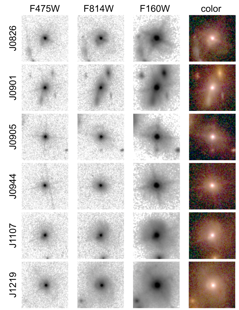
Figure 2: Left to right: HST/WFC3 images in the UVIS/F475W, UVIS/F814W, and IR/F160W bands for 6/12 galaxies. The three images for each galaxy are combined in the rightmost column to produce a blue-green-red color composite. Each image is 6$\arcsec$ across, which corresponds to $\approx 40$ kpc at the median redshift of the sample, and is oriented such that north is up and east is to the left. Top to bottom: images for J0826, J0901, J0905, J0944, J1107, and J1219.

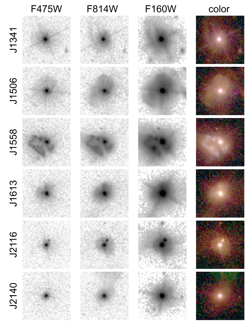
Figure 3: Left to right: HST/WFC3 images in the UVIS/F475W, UVIS/F814W, and IR/F160W bands for 6/12 galaxies. The three images for each galaxy are combined in the rightmost column to produce a blue-green-red color composite. Each image is 6$\arcsec$ across, which corresponds to $\approx 40$ kpc at the median redshift of the sample, and is oriented such that north is up and east is to the left. Top to bottom: images for J1341, J1506, J1558, J1613, J2116, and J2140.

4 Morphological and Photometric Analysis

As described by Diamond-Stanic et al. (2012) and Sell et al. (2014), a key challenge in quantifying the photometric and morphological characteristics of these galaxies based on HST imaging is that the half-light radii inferred from single-component models with GALFIT (Peng et al., 2002, 2010) are often comparable to, or even smaller than, the width of a single pixel. In other words, the two-dimensional light profiles of these galaxies on scales smaller than a kiloparsec are dominated by the width and shape of the point-spread function. This can be seen in Figure 2 and Figure 3 in which the central source dominates the central pixels in each image. These images are $6\arcsec$ on a side, whereas the median half-light radius measured from the UVIS images is $0.02\arcsec$ (see Section 4.1 and Table 2). For comparison, the pixel values in the central $0.2\arcsec\times 0.2\arcsec$ region of each F475W and F814W image ($\textnormal{FWHM}\approx 0.07\arcsec$) and the central $0.4\arcsec\times 0.4\arcsec$ of each F160W image ($\textnormal{FWHM}\approx 0.15\arcsec$) exceed the maximum scale parameter used to produce the figures (i.e., these pixels are completely black in Figure 2 and Figure 3). Therefore, our desire to understand the intrinsic light profile down to $\sim 0.1$ kpc scales requires the use of an empirically-generated PSF and modeling of the observed light profile to infer information about regions that are smaller than the PSF FWHM.

Regarding photometric measurements, our goal is to perform photometry on the same morphological component in each image: the compact central starbursts that were found by Diamond-Stanic et al. (2012) and Sell et al. (2014) to dominate the light profile in rest-frame optical images and inferred to have sizes as small as $r_{e}\sim 100$ pc. From that perspective, our morphological and photometric analyses of the central source in each galaxy are driven by the goals of (1) finding an accurate size estimate for the central source, and (2) measuring the flux of this source on the same physical scale in all three images.

Regarding the estimate of the half-light radius, we focus on the UVIS bands (F475W, F875W), which have the best spatial resolution and which are the most clearly dominated by the central source (see Section 4.1). The increased prominence of non-nuclear, extended emission at longer wavelengths is clear from Figure 2 and Figure 3. This is a signature of an extended stellar population that is older and redder than the central starburst (see Section 5.2). To facilitate measurements on the same physical scale in each image, we perform a simultaneous fit to all three photometric bands, using the half-light radius for the central component measured from the UVIS bands (see Section 4.1) as a fixed constraint for all images (see Section 4.2).

4.1 Measuring the half-light radius of the central component with GALFIT

For our measurements of half-light radius, we perform fits to both the F475W and F814W images using the GALFITM software developed by the MegaMorph collaboration (Häußler et al., 2013; Vika et al., 2013). This software creates model images in multiple bands and then convolves each model image with a PSF before comparing with the data, minimizing residuals using the Levenberg-Marquardt method (Peng et al., 2002). To generate the empirical PSF for each image, we use stars from the same image and the method described by Sell et al. (2014). For this analysis, we use the $0.025\arcsec$/pixel images, which have the best spatial sampling of the central source. Following Diamond-Stanic et al. (2012) and Sell et al. (2014), we use single-component Sérsic profiles with $n=4$ (de Vaucouleurs, 1948; Sérsic, 1963). To quantify the values and uncertainties for half-light radii ($r_{e}$) and magnitudes ($m_{\textnormal{\scriptsize{F475W}}}$, $m_{\textnormal{\scriptsize{F814W}}}$), we generate a suite of models with GALFITM over a grid of $r_{e}$, $m_{\textnormal{\scriptsize{F475W}}}$, and $m_{\textnormal{\scriptsize{F814W}}}$ for each galaxy. To provide initial estimates for these values, we perform simultaneous fits to the F475W and F814W images using a square image region that is $200\times 200$ pixels or $5\arcsec$ on a side; this corresponds to $\sim 30$ kpc at the median redshift of our sample, so this initial region encompasses the vast majority of the emission for each galaxy. For this multi-band analysis, we use the same $r_{e}$, position angle, and axis ratio values for both the F475W and F814W images.

For our subsequent analysis, we focus on the central region ($0.5\arcsec\times 0.5\arcsec$ or $\approx 3~{}\textnormal{kpc}\times 3$ kpc) of each galaxy for which the diffraction pattern from the central source dominates the light profile. This allows the data vs model comparison to be based on pixels that do not have significant contributions from tidal and other extended features. For our model comparisons, we use a set of 9 magnitude values ranging from 0.2 mag fainter to 0.2 mag brighter than the initial estimate from GALFITM. We also use a set of 9 $r_{e}$ values ranging from $3\times$ smaller to $3\times$ larger than the initial estimate. Holding $m_{\textnormal{\scriptsize{F475W}}}$, position angle, and axis ratio fixed, we calculate $\chi^{2}/\nu$ across this $9\times 9$ grid of $m_{\textnormal{\scriptsize{F814W}}}$ and $r_{e}$ values. We then repeat with $m_{\textnormal{\scriptsize{F814W}}}$ fixed, using a grid of $m_{\textnormal{\scriptsize{F475W}}}$ and $r_{e}$. We construct contours of $\Delta\chi^{2}$ in each magnitude–size parameter space, and we identify the 68% range for $r_{e}$ based on $\Delta\chi^{2}=2.3$ (Avni, 1976; Wall & Jenkins, 2003). The best-fit values and 68% limits for $r_{e}$ are very similar for the $m_{\textnormal{\scriptsize{F814W}}}$–$r_{e}$ and $m_{\textnormal{\scriptsize{F475W}}}$–$r_{e}$ grids, and we report the average of the best-fit values and the uncertainty based on the minimum and maximum limits in Table 2. To provide additional information about the uncertainty on the $r_{e}$ estimates and the differences between the F475W and F814W images, we also calculate $\chi^{2}/\nu$ for each image individually and report the best-fit values in Table 2.

We find half-light radii that are remarkably small ($r_{e}=0.01\arcsec$–$0.03\arcsec$ for most galaxies), with typical statistical uncertainties of $20\%$–$30\%$. In addition, we find that the half-light radii estimated from the F475W images are systematically smaller than those estimated from the F814W images, by about 40% on average. This difference between F475W and F814W $r_{e}$ values is comparable to the width of the 68% confidence interval on $r_{e}$ from the multi-band analysis, and it provides an additional diagnostic of the uncertainty for these $r_{e}$ estimates. As described above (and shown in Figure 2 and Figure 3), the images at shorter wavelengths have less extended emission, such that the two-dimensional light profiles are more dominated by the central source for the F475W images compared to the F814W images. In other words, our model assumption that the observed light profile can be described by a single component is most appropriate for the F475W images, and the additional extended emission at F814W appears to be driving the model towards larger $r_{e}$ values. While this suggests that the smaller $r_{e}$ values estimated from the F475W images might be closest to the “true” values, we adopt the more conservative estimate of $r_{e}$ from the joint fit to both UVIS bands, which gives values that are larger than the F475W-only estimate and smaller than the F814W-only estimate (i.e., smaller than F814W-only values from previous work: Diamond-Stanic et al., 2012; Sell et al., 2014). In Table 2, we quantify these differences for each galaxy relative to the fiducial $r_{e}$ value from a joint fit.

Table 2: Half-light radius measurements for the central component from GALFITM

	$r_{e,central}$ [$\arcsec$]
Galaxy	UVIS	F475W	F814W
J0826	$0.0151\pm 0.0031$	0.0122 ($-19\%$)	0.0201 ($+33\%$)
J0901	$0.0149\pm 0.0033$	0.0103 ($-31\%$)	0.0235 ($+58\%$)
J0905	$0.0105\pm 0.0027$	0.0095 ($-9\%$)	0.0117 ($+12\%$)
J0944	$0.0099\pm 0.0030$	0.0072 ($-28\%$)	0.0137 ($+37\%$)
J1107	$0.0156\pm 0.0041$	0.0112 ($-28\%$)	0.0238 ($+53\%$)
J1219	$0.0257\pm 0.0038$	0.0216 ($-16\%$)	0.0299 ($+16\%$)
J1341	$0.0127\pm 0.0023$	0.0119 ($-6\%$)	0.0138 ($+9\%$)
J1506	$0.0118\pm 0.0025$	0.0089 ($-24\%$)	0.0160 ($+36\%$)
J1558	$0.0387\pm 0.0064$	0.0286 ($-26\%$)	0.0573 ($+48\%$)
J1613	$0.1289\pm 0.0157$	0.1072 ($-17\%$)	0.1604 ($+24\%$)
J2116	$0.0216\pm 0.0046$	0.0171 ($-21\%$)	0.0253 ($+17\%$)
J2140	$0.0145\pm 0.0045$	0.0077 ($-47\%$)	0.0262 ($+81\%$)

Note. — Column 1: Short SDSS name (see Table 1). Column 2: Half-light radius for the central component in arcseconds estimated from a joint fit to the F475W and F814W images. The uncertainty represents a 68% confidence interval (see Section 4.1). The median uncertainty is 21%. Column 3: Best-fit half-light radius based on the F475W images. The quantity in parentheses indicates the percent difference relative to the half-light radius from Column 2. The median difference is $-23$%. Column 4: Best-fit half-light radius based on the F814W images. The quantity in parentheses indicates the percent difference relative to the half-light radius from Column 2. The median difference is $+35$%.

4.2 Three-band photometry of the central source

For our three-band photometry of the central source, we use the $r_{e}$ values measured from the UVIS images as a fixed constraint for simultaneous model fits to the F475W, F814W, and F160W images. For this analysis, we use the $0.05"$/pixel images because this allows us to incorporate the F160W images and it provides the same pixel sampling in all three images. To measure this photometry and uncertainty, which is based on the total flux from model Sersic profiles, we use a method similar to that described above in Section 4.1. For each magnitude ($m_{\textnormal{\scriptsize{F475W}}}$, $m_{\textnormal{\scriptsize{F814W}}}$, $m_{\textnormal{\scriptsize{F160W}}}$) for each galaxy, we generate GALFITM models over a set of 9 magnitude values ranging from 0.2 mag fainter to 0.2 mag brighter than our initial estimate. We then calculate $\chi^{2}/\nu$ across a $9\times 9$ grid of $m_{\textnormal{\scriptsize{F475W}}}$ and $m_{\textnormal{\scriptsize{F814W}}}$ and across a $9\times 9$ grid of $m_{\textnormal{\scriptsize{F814W}}}$ and $m_{\textnormal{\scriptsize{F160W}}}$, and we determine the best-fit magnitude and 68% range based on contours of $\Delta\chi^{2}$. We apply corrections for Galactic extinction based on $E(B-V)$ color excess values from the Schlegel et al. (1998) infrared dust maps, using the Schlafly & Finkbeiner (2011) calibration for $R_{V}=3.1$ and the Fitzpatrick (1999) reddening law. We report the calibrated photometry of the central component in Table 3. As we discuss further in Section 5, the [F475W]$-$[F814W] and [F814W]$-$[F160W] colors are quite blue, implying young ages for the underlying stellar population.

Table 3: Photometric measurements of the central source from GALFITM

Galaxy	F475W	F814W	F160W
J0826	$19.402\pm 0.069$	$19.050\pm 0.061$	$18.801\pm 0.034$
J0901	$19.330\pm 0.057$	$18.944\pm 0.065$	$18.639\pm 0.038$
J0905	$19.428\pm 0.059$	$19.065\pm 0.061$	$18.937\pm 0.044$
J0944	$19.731\pm 0.068$	$19.165\pm 0.070$	$18.674\pm 0.033$
J1107	$19.380\pm 0.061$	$19.095\pm 0.071$	$18.949\pm 0.040$
J1219	$19.646\pm 0.064$	$18.823\pm 0.061$	$18.379\pm 0.038$
J1341	$18.910\pm 0.046$	$18.756\pm 0.056$	$18.960\pm 0.044$
J1506	$19.074\pm 0.050$	$18.907\pm 0.056$	$18.807\pm 0.036$
J1558	$19.611\pm 0.064$	$19.263\pm 0.070$	$18.791\pm 0.040$
J1613	$19.451\pm 0.073$	$18.574\pm 0.059$	$17.900\pm 0.033$
J2116	$19.591\pm 0.089$	$19.099\pm 0.066$	$19.135\pm 0.045$
J2140	$19.923\pm 0.092$	$19.165\pm 0.084$	$18.992\pm 0.044$

Note. — Column 1: Short SDSS name (see Table 1). Columns 2–4: Calibrated photometry in AB magnitudes for the central component of each galaxy in the F475W, F814W, and F160W images. This is based on a joint-fit to the same morphological component in all three bands, as described in Section 4.2. These values have been corrected for Galactic extinction. The uncertainty represents a 68% confidence interval.

Table 4: Central and total half-light radius

Galaxy	$r_{e,central}$ [kpc]	$r_{e,total}$ [kpc]
J0826	$0.101\pm 0.021$	$0.173^{+0.075}_{-0.053}$
J0901	$0.087\pm 0.019$	$0.237^{+0.144}_{-0.088}$
J0905	$0.076\pm 0.019$	$0.097^{+0.044}_{-0.033}$
J0944	$0.061\pm 0.019$	$0.114^{+0.067}_{-0.047}$
J1107	$0.092\pm 0.024$	$0.273^{+0.192}_{-0.112}$
J1219	$0.148\pm 0.022$	$0.412^{+0.194}_{-0.124}$
J1341	$0.088\pm 0.016$	$0.117^{+0.040}_{-0.032}$
J1506	$0.079\pm 0.017$	$0.168^{+0.076}_{-0.054}$
J1558	$0.209\pm 0.034$	$0.778^{+0.383}_{-0.244}$
J1613	$0.741\pm 0.090$	$0.949^{+0.274}_{-0.207}$
J2116	$0.157\pm 0.033$	$0.284^{+0.131}_{-0.092}$
J2140	$0.107\pm 0.033$	$0.153^{+0.092}_{-0.064}$

Note. — Column 1: Short SDSS name (see Table 1). Column 2: Half-light radius for the central component in kpc estimated from a joint fit to the F475W and F814W images (see Section 4.1 and Table 2). The uncertainty represents a 68% confidence interval, and the median fractional uncertainty is 21%. Column 3: Estimate of half-light radius for the entire galaxy based on the F814W images. This involves extrapolating the $n=4$ Sersic model until it reaches 50% of the total light from the galaxy. The upper and lower limits account for the uncertainty on this extrapolation, including uncertainty on the central $r_{e}$ value, the central flux, and the total flux. The median difference for the lower limit is $-32\%$ and the median difference for the upper limit is $+47\%$.

4.3 Estimating half-light radius for the entire galaxy

The analysis described above provides measurements of the half-light radius and three-band photometry for the central component of each galaxy, which typically contributes $\approx 75\%$ of the total light at F814W and $\approx 90\%$ of the total light at F475W. Because there is significant residual emission, the half-light radius for the central component contains less than half of the light for the entire galaxy. To provide an estimate of $r_{e}$ that is more appropriate for the total light from each galaxy, we extrapolate the $n=4$ Sersic model until it reaches half of the total flux measured using the F814W images in circular apertures with 25 kpc diameters. We account for uncertainties on this extrapolation based on the flux uncertainty for the central and total components, which impacts how far one needs to extrapolate the central light profile. In practice, this estimate of total half-light radius is larger than the central half-light radius by a factor of two on average, which is similar to the ratio $r_{70}/r_{50}=2.08$ for an $n=4$ Sersic model. We report these values in Table 4. For the remainder of the paper, we use $r_{e,central}$ to refer to the half-light radius of the central component and $r_{e,total}$ to refer to this larger estimate of total half-light radius.

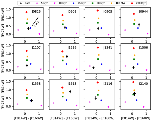
Figure 4: Plots of observed-frame [F475W]$-$[F814W] and [F814W]$-$[F160W] colors for each of the 12 galaxies in the sample. Each panel shows the observed colors for one galaxy and for SSP models at the galaxy’s redshift with ages between $t=5$ Myr and $t=200$ Myr. The arrow in the top-left panel shows the impact of dust attenuation with optical depth $\hat{\tau}=1$ at $\lambda_{\textnormal{\scriptsize{rest}}}=5500$ Å, which corresponds to $A_{V}=1.086$ mag. While many galaxies are consistent with ages between $t=25$ Myr and $t=50$ Myr, the bluest galaxies (e.g., J1341, J1506) clearly require $t<10$ Myr.

5 Stellar population modeling

The multi-band photometry of the compact stellar population in each galaxy allows us to estimate the stellar mass associated with these recently formed stars. For comparison, the spatially integrated (i.e., unresolved) photometry of these galaxies, as described in Section 5.2 and used in previous studies (e.g., Diamond-Stanic et al., 2012; Rupke et al., 2019), includes two ultraviolet bands from the Galaxy Evolution Explorer (GALEX, Martin et al., 2005; Morrissey et al., 2007, far-ultraviolet FUV and near-ultraviolet NUV), five optical bands from the SDSS (ugriz), and four infrared bands from the Wide-field Infrared Survey Explorer (WISE, Wright et al., 2010, W1, W2, W3, W4). In contrast, the spatially resolved photometry from HST is limited to three bands. This presents a challenge for performing detailed stellar population synthesis modeling with a large range of free parameters that describe the star-formation history and dust properties (e.g., Conroy, 2013).

In this context, we begin by considering simple stellar population (SSP) models from FSPS (Flexible Stellar Population Synthesis: Conroy et al., 2009; Conroy & Gunn, 2010) to gain insight on parameters such as stellar mass and stellar age. Given that we are primarily interested in determining the properties of the stars that formed within the central several hundred parsecs during a recent starburst event, this idealized assumption of a single-age central stellar population provides useful constraints. To visualize the range of SSP ages that are consistent with our nuclear photometry, we use FSPS to compute the expected [F475W]$-$[F814W] and [F814W]$-$[F160W] observed-frame colors for a grid of models with ages between $t=5$ Myr and $t=200$ Myr at the redshift of each of our 12 galaxies. This comparison avoids the need to make $K$-corrections (e.g., Hogg et al., 2002; Blanton & Roweis, 2007) to compute magnitudes and colors in a common set of rest-frame filters.

As shown in Figure 4, we find that all 12 galaxies are consistent with light-weighted stellar ages for their central starburst components in the range $t=5$–50 Myr. At least two galaxies (J1341, J1506) clearly require a central stellar age $t<10$ Myr, and a few other galaxies (J0905, J1107, J2116) have blue colors that also suggest very young stellar ages (i.e., implying a starburst event within the last 10 Myr). A number of galaxies (J0826, J0901, J0944, J1558) have colors that are consistent with a $t\approx 25$ Myr stellar population with small dust attenuation, and the remaining galaxies with the reddest [F475W]$-$[F814W] colors (J1219, J1613, J2140) are consistent with more dust attenuation and/or older ages $t\approx 50$ Myr. As a preliminary estimate, we compute the stellar mass associated with a $t=25$ Myr SSP at solar metallicity, scaled to match the F814W observed-frame luminosity for each galaxy. This yields a median value of $\log(\mathcal{M}_{*}{}_{,central})=10.3$, which matches the median value we find from our more detailed analysis below (see Section 5.1). For reference, forming this amount of stellar mass over a timescale of 25 Myr implies an average star-formation rate of $\approx 800~{}\mathcal{M}_{\odot}/\textnormal{yr}^{-1}$. This value is large, but it is within the range of previously published star-formation rates for this sample based on infrared luminosity and SED modeling (e.g., Diamond-Stanic et al., 2012; Geach et al., 2013; Sell et al., 2014; Geach et al., 2014, 2018).

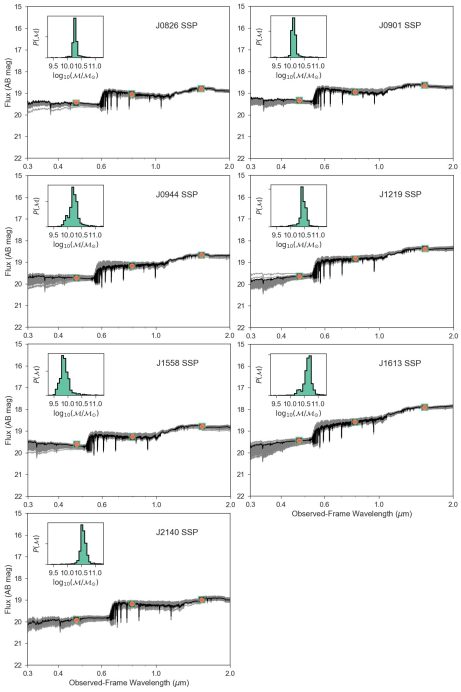
Figure 5: Results from SSP model fits to the nuclear SEDs for the 7/12 galaxies that are consistent with ages $t\geq 25$ Myr for their central component. The main panels show the observed nuclear SEDs (orange circles), a random sampling ($n=100$) of the SSP models considered by Prospector (gray shading), the maximum-likelihood SSP model (black line), and model photometry for the maximum-likelihood model (green boxes). The inset panels show the stellar mass posteriors from Prospector. In all seven cases, the SSP models provide reasonable fits to the photometry and the stellar mass is well constrained.

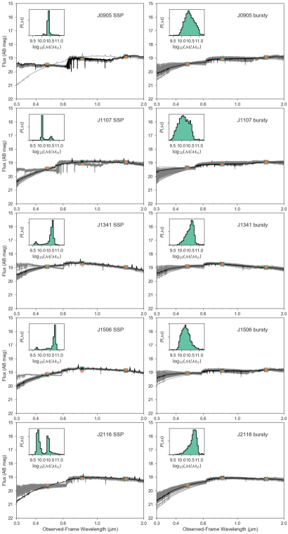
Figure 6: Results from stellar population modeling for the 5/12 galaxies with the bluest colors, which suggest significant contributions from stars with $t\leq 10$ Myr. Each panel shows an observed nuclear SED (orange circles), a random sampling ($n=100$) of the models considered by Prospector (gray shading), the maximum-likelihood model (black line), and model photometry for the maximum-likelihood model (green boxes), while the inset panel show the stellar mass posterior. Left: Results from SSP models, for which the model fits and the posterior distributions show degeneracies. The models with stronger Balmer breaks are older, less dusty, and less massive, while the models with weaker Balmer breaks are younger, more dusty, and more massive. Right: The same SEDs with model fits for a more flexible star-formation history: a delayed-$\tau$ model with a late-time burst. These models more robustly characterize the range of potential SEDs and the uncertainty on the stellar mass.

5.1 Probability distributions for central stellar mass

With the goal of quantifying posterior probability distributions for stellar mass, we use Prospector (Leja et al., 2017; Johnson et al., 2019) with model assumptions and prior probabilities informed by the SSP comparisons above. Within Prospector, we use the dynesty package (Speagle, 2020), which estimates Bayesian posteriors using dynamic nested sampling. We begin with SSP models ($\textnormal{sfh}=0$ in FSPS) fixed at solar metallicity, and we adopt a prior probability on age that is flat in logarithmic spacing between 3 Myr and 100 Myr, informed by the blue colors and young ages found above. We also implement dust attenuation as a power law ($\textnormal{dust\_type}=0$ in FSPS) with the optical depth $\hat{\tau}\propto\lambda^{-0.7}$ (Charlot & Fall, 2000).

We find that the galaxies with less extreme colors (i.e., those that are consistent with $t\geq 25$ Myr) have nuclear SEDs that can be well described by single-age SSP models. In Figure 5, we show the observed photometry, model photometry, model SEDs, and stellar mass posterior distributions for the galaxies J0826, J0901, J0944, J1219, J1558, J1613, and J2140. The width of the stellar mass posterior between the 16th and 84th percentiles (i.e., corresponding to a 68% confidence interval) ranges from 0.09 dex to 0.25 dex for these seven galaxies. The posterior distributions are also single-peaked and reasonably symmetrical, indicating that the stellar mass value is well constrained.

In contrast, the nuclear SEDs of galaxies with the bluest colors (consistent with $t<10$ Myr) are not fit robustly by single-age SSP models. In particular, there is degeneracy between SSP model ages that is evident in the range of SSP model fits. We show SSP model fits on the left-hand side of Figure 6, and we find comparable fits to the photometry for models that are different in age by almost an order of magnitude (e.g., $t\approx 4$ Myr vs $t\approx 30$ Myr for J2116). For all five galaxies, this degeneracy is between models with stronger Balmer breaks (which are older, less dusty, and less massive) compared to models with weaker Balmer breaks (which are younger, more dusty, and more massive). This degeneracy is also evident in the asymmetries and multiple peaks in the stellar mass posteriors (e.g., the width of the stellar mass posterior between the 16th and 84th percentiles is larger than 0.5 dex for galaxies J1107 and J2116).

To provide more robust constraints on the central stellar mass for these younger and bluer galaxies, we explore models with more flexible star-formation histories. In particular, we use delayed-$\tau$ models ($\textnormal{sfh}=4$ in FSPS) for the star formation history ($\textnormal{SFR}\propto te^{-t/\tau}$) with additional parameters to characterize a recent burst of star formation, including the time at which the burst happens and the fraction of the total stellar mass formed in the burst. This approach is very similar to the stellar population modeling described by Rupke et al. (2019). In the right panel of Figure 6, we show that these models are clearly capable of fitting the photometry. The stellar mass posterior distributions are often broader than those for SSP models, reflecting how the more flexible models have a broader range of parameters that are consistent with the photometry. Compared to results from SSP modeling, this provides constraints on stellar mass that are less sensitive to uncertainties in the star-formation history. The difference between the median of the stellar mass posterior and the 16th and 84th percentile values is $\pm 0.2$ dex or $\pm 0.3$ dex for all five galaxies. In comparing the posterior median values between the SSP models and the delayed-$\tau$ models with bursts, the values agree within 0.1 dex for J0905, J1107, and J1341. In contrast, there are large differences for J1506 (0.6 dex) and J2116 (0.8 dex), both of which have more robust constraints from the more flexible models.

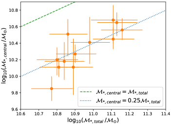
Figure 7: The relationship between central stellar mass and total stellar mass. The central stellar mass is estimated from spatially resolved nuclear SEDs, and the total stellar masses is estimated from spatially unresolved total SEDs. The vast majority of the sample is consistent with $\mathcal{M}_{*}{}_{,central}/\mathcal{M}_{*}{}_{,total}\approx 0.25$.

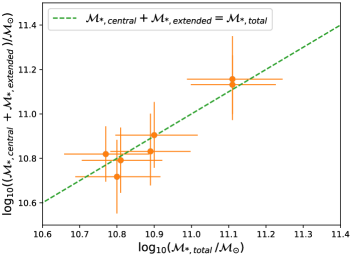
Figure 8: A comparison between measurements of central stellar mass $+$ extended stellar mass from spatially resolved SEDs (using HST data) and independent measurements of total stellar mass from spatially unresolved SEDs (not using HST data). This focuses on the seven galaxies in Table 8 with the smallest uncertainties on F475W extended flux. These two methods for estimating the total stellar mass agree well within the uncertainties.

5.2 Comparing to the Total Stellar Population

Our analysis of the central stellar population can be combined with analysis of the total stellar population to determine the fraction of the total stellar mass associated with the compact starburst component. To estimate the total stellar mass, we make use of publicly available photometric measurements at ultraviolet (GALEX Release 7), optical (SDSS Data Release 15, Aguado et al., 2019), and infrared (unWISE, Lang, 2014; Lang et al., 2016) wavelengths. We use the modelMag photometry from SDSS, calibrated magnitudes from GALEX, and the unWISE forced photometry based on SDSS positions. For galaxies without GALEX fuv_mag values (J0944, J1219, J2116), we use GALEX FUV fluxes measured at the NUV positions. We focus on the WISE W1 and W2 bands (central wavelengths 3.4 and 4.6 $\mu$m) because these wavelengths are dominated by stellar emission, and we do not include the W3 and W4 bands (central wavelengths 12 and 22 $\mu$m) in our stellar population analysis because these wavelengths are dominated by dust emission. The total SEDs span an observed wavelength range 0.15–4.6 $\mu$m (corresponding to $\lambda_{\textnormal{\scriptsize{rest}}}=0.10$–2.9 $\mu$m at the median redshift of our sample). We apply corrections for Galactic extinction in each band based on extinction coefficients from Yuan et al. (2013) for the Fitzpatrick (1999) reddening law with 14% corrections to $E(B-V)$ values from Schlegel et al. (1998).

For the stellar population modeling with Prospector, we use a delayed-$\tau$ model with a late-time burst for the star-formation history. We impose a lower limit on stellar age (i.e., how long ago the galaxy began forming stars) of 1 Gyr and an upper limit of 7 Gyr, which is approximately the age of the universe at $z=0.75$, the highest redshift in the sample. We also allow up to 50% of the stars to have formed in the recent burst of star formation. We report the constraints on stellar mass ($\mathcal{M}_{*}$), stellar age ($t_{age}$), the e-folding parameter ($\tau$), the burst fraction ($f_{burst}$), and the time of the burst expressed as a fraction of the stellar age ($f_{age,burst}$) in Table 7. For the total stellar mass posteriors, we find a median for the 50th percentile values across the sample of $\log(\mathcal{M}_{*}/\mathcal{M}_{\odot})=10.9$. In comparison, the median for the central stellar mass posteriors was $\log(\mathcal{M}_{*}/\mathcal{M}_{\odot})=10.3$. We show the relationship between central stellar mass and total stellar mass in Figure 7. The vast majority of the galaxies (11/12) are consistent with $\mathcal{M}_{*}{}_{,central}/\mathcal{M}_{*}{}_{,total}\approx 0.25$. The only exception is J1558 ($\mathcal{M}_{*}{}_{,central}/\mathcal{M}_{*}{}_{,total}\approx 0.12$), which is an ongoing merger (see Section 2 and Figure 3) that is the least dominated by a single source (e.g., it has a lot of extended emission, including a second, fainter nucleus).

As a consistency check, we also use the HST images to measure the fluxes and colors of the extended, non-nuclear emission in each galaxy with the goal of measuring the extended stellar mass. We do this by subtracting the central Sersic photometry from the total galaxy photometry measured in apertures with 25 kpc diameters. In practice, the uncertainties on these extended fluxes can be large, especially in the UVIS bands, because the median ratio of central flux to total flux is 93% at F475W, 75% at F814W, and 66% at F160W. The typical $\approx 6\%$ uncertainty on the central fluxes in the UVIS bands then propagates into a much larger fractional uncertainty for the fainter extended flux. Focusing on the seven galaxies with the smallest uncertainties on their extended F475W flux, we carry out a stellar population analysis based on extended emission in the F475W, F814W, and F160W images. We use delayed-$\tau$ star-formation histories with parameters to characterize a more recent burst, and we show the constraints on stellar population parameters in Table 8. We compare $\mathcal{M}_{*}{}_{,central}+\mathcal{M}_{*}{}_{,extended}$ estimated from the spatially resolved HST photometry to $\mathcal{M}_{*}{}_{,total}$ estimated from spatially integrated photometry in Figure 8, and these two methods of estimating the total stellar mass show very good agreement.

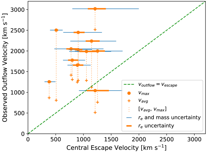
Figure 9: A comparison between observed outflow velocity and central escape velocity. The average outflow velocity is based on the median of the cumulative equivalent width distribution for the $\textrm{Mg}~{}\textsc{ii}~{}\lambda\lambda 2796,2803$ doublet (see Table 1); the maximum outflow velocity is based on the point where the equivalent width distribution for Mg ii $\lambda 2796$ reaches 95% of the total (see Table 1); and the central escape velocity is based on central stellar mass and effective radius (see Equation 1). The maximum outflow velocity exceeds the central escape velocity for 11/12 galaxies, and the median ratio is $v_{max}/v_{esc,central}=2.2$. The average outflow velocity exceeds the central escape velocity for 9/12 galaxies, and the median ratio is $v_{avg}/v_{esc,central}=1.5$. This significant excess of outflow velocity relative to escape velocity has important implications for the physical mechanisms responsible for driving the fast outflows and for the fate of the outflowing gas (see Section 6).

6 Discussion

The primary motivation for obtaining these multi-band imaging data was to test physical mechanisms that could launch outflows (1) at speeds significantly faster than the central escape velocity or (2) at speeds comparable to the central escape velocity. In Diamond-Stanic et al. (2012), we found evidence for star-formation rate surface densities that approach the Eddington limit ($\Sigma_{\textnormal{\scriptsize{SFR}}}\sim 3000$ M_⊙ yr^-1 kpc^-2; Murray et al., 2005; Thompson et al., 2005; Hopkins et al., 2010) and we pointed out that if the stellar mass profile matched the observed light profile, then it would be possible to have escape velocities that were comparable to the observed outflow velocities. This would have been consistent with scenario (2) and models of radiation-driven winds that predict outflow velocities near the escape velocities of the densest stellar systems within a galaxy (e.g., Murray et al., 2011). In contrast, our new results (see below and Figure 9) are consistent with scenario (1) and models that can produce $>1000$ km s^-1 outflows that exceed the central escape velocity by a significant factor (e.g., Heckman et al., 2011; Thompson et al., 2015; Bustard et al., 2016). In other words, the fact that the compact starburst component contributes 25% to the total stellar mass implies that 10%–15% of the total stellar mass is within the half-light radius (i.e., half the mass of the compact starburst is within the half-light radius). This yields values for central escape velocity (Section 6.1) and central stellar surface density (Section 6.2) that require scenario (1) to explain the fast outflows. We explore this comparison with outflow models in more detail in Section 6.5.

6.1 Constraints on Central Escape Velocity

We can combine the measurements of half-light radius (Table 2, Section 4.1) with the measurements of central stellar mass (Table 5, Table 6, Section 5.1) to estimate a central escape velocity for each galaxy.

$$v_{esc,central}=\sqrt{G\mathcal{M}_{*}{}_{,central}/r_{e,central}}$$ (1)

This form of Equation 1 uses the entire stellar mass of the central stellar population, and it assumes that half of that mass is within the half-light radius. Based on this calculation, we find a median value of $v_{esc,central}=900$ km s^-1, which is very similar to the estimated central escape velocity of the Milky Way on $r=0.1$ kpc scales (e.g., Kenyon et al., 2008; Brown, 2015).

We compare these estimates of central escape velocity with observed outflow velocity in Figure 9. We use the lower limits on $r_{e,central}$ and upper limits on $\mathcal{M}_{*}{}_{,central}$ to calculate upper limits on $v_{esc,central}$, and we use the opposite limits on size and mass to calculate lower limits on $v_{esc,central}$. We also show the portion of the uncertainty on $v_{esc,central}$ and that comes from the upper and lower limits on $r_{e,central}$. When characterizing the outflow velocity by $v_{max}$ (defined by the point at which the equivalent width distribution for $\textrm{Mg}~{}\textsc{ii}~{}\lambda 2796$ reaches 95% of the total, see Table 1) we find that 11/12 galaxies have observed outflow velocities that clearly exceed their central escape velocities, with a median $v_{max}/v_{esc,central}=2.2$ for the full sample. The only galaxy consistent with $v_{max}=v_{esc,central}$ is J2140, which has the slowest outflow speed in the sample and is also the only galaxy with evidence for a non-zero AGN continuum contribution at near-ultraviolet wavelengths (see Section 2). This contribution could bias the $r_{e,central}$ estimate to be low for J2140 (especially when considering the F475W band, see Table 2) and the $v_{esc,central}$ estimate to be high. If we used the $r_{e,central}$ value based solely on F814W, this galaxy would have a best-fit ratio $v_{max}/v_{esc,central}=1.15$, but it would still be consistent with $v_{max}=v_{esc,central}$ given the uncertainties. Regardless, this does not impact our estimate of the median $v_{max}/v_{esc,central}$ ratio for the sample.

We also find that the average outflow velocity $v_{avg}$ (defined by the median of the cumulative equivalent width distribution for $\textrm{Mg}~{}\textsc{ii}~{}\lambda\lambda 2796,2803$, see Table 1) exceeds the best-fit central escape velocity for 9/12 galaxies, with $v_{avg}/v_{esc,central}=1.5$ as the median ratio for the full sample. This implies that the bulk of the outflowing gas in the vast majority of these galaxies has sufficient momentum to easily escape from the central regions of the galaxy. Given the typical outflow velocities $\overline{v_{max}}=2000$ km s^-1and $\overline{v_{avg}}=1200$ km s^-1 for this sample, and the fact that several of these galaxies are known to have extended molecular outflows on several kpc scales (Geach et al., 2018) to 10 kpc scales (Geach et al., 2014), these ionized outflows are also clearly capable of escaping the galaxy into the circumgalactic medium (e.g., the $r=10$–50 kpc ionized outflows found by Rupke et al., 2019). Unless forces besides gravity are able to slow them down, they would also escape their $10^{12-13}~{}\mathcal{M}_{\odot}$ dark matter halos (e.g., Moster et al., 2013; Muratov et al., 2015).

Figure 10: A comparison between observed outflow velocity and central stellar surface density. This is based on $v_{max}$ outflow velocities (Table 1), $\Sigma_{e,central}$ surface densities within the half-light radius (Equation 2), and $\Sigma_{1}$ surface densities within the central kpc (calculated as lower limits using Equation 4). There is no apparent relationship between outflow velocity and stellar surface density in our sample. The median value $\Sigma_{e,central}=3\times 10^{11}$ M_⊙ kpc^-2 on $r=0.1$–0.2 kpc scales matches theoretical estimates of the Eddington limit (e.g., Hopkins et al., 2010), while the median value $\Sigma_{1}=7\times 10^{9}$ M_⊙ kpc^-2 on $r=1$ kpc scales is consistent with values for compact galaxies at $0.5<z<3.0$ (e.g., Barro et al., 2017).

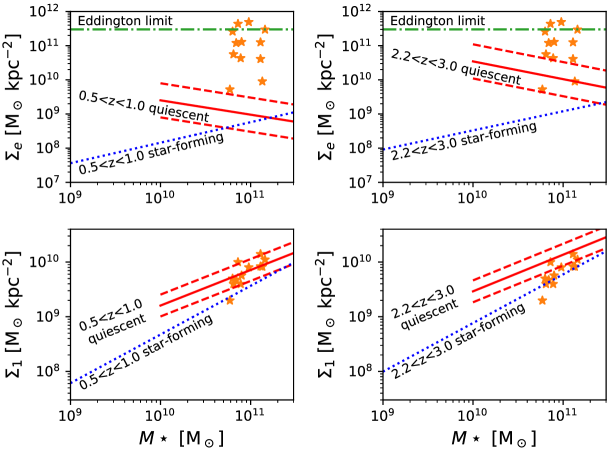
Figure 11: The relationship between stellar mass surface density and stellar mass. The points for our sample are based $\Sigma_{e,total}$ values on $r=0.2$–0.3 kpc scales (Equation 3), $\Sigma_{1}$ values on $r=1$ kpc scales (calculated as lower limits using Equation 4), and total stellar mass values (see Table 1 and Table 7). The solid red and dotted blue lines illustrate the relations for quiescent and star-forming galaxies at $0.5<z<3.0$ from Barro et al. (2017). The top panels show $\Sigma_{e}$, the bottom panels show $\Sigma_{1}$, the left panels show relations at $0.5<z<1.0$ (overlapping with our sample), and the right panels show relations at $2.2<z<3.0$ (the highest redshift available). In the top panels, the green dash-dot line corresponds to the theoretical estimate of the Eddington limit from Hopkins et al. (2010). The data for the galaxies in our sample are the same for both the left and right panels. In terms of $\Sigma_{e}$, 10/12 galaxies in our sample (see Section 6.3 for details) lie significantly above the relations found by Barro et al. (2017) at all redshifts. In terms of $\Sigma_{1}$, there is good agreement between our lower-limit values and the relation for $0.5<z<1.0$ quiescent galaxies, although several of our galaxies extend slightly above the scatter at $0.5<z<1.0$ and are closer to the relation for $2.2<z<3.0$ quiescent galaxies. This shows that our galaxies are extreme in terms of $\Sigma_{e}$, but their more modest $\Sigma_{1}$ values are consistent with those of compact massive galaxies from the literature.

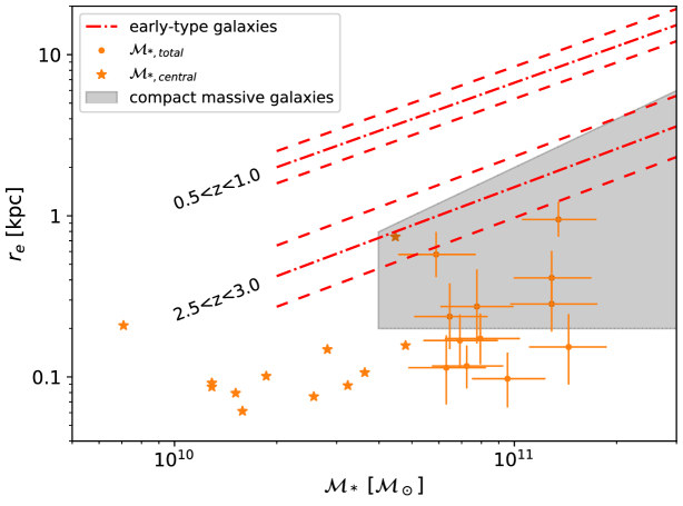
Figure 12: The relationship between half-light radius and stellar mass. For our sample, the values for $r_{e,total}$ and total stellar mass are shown as the circles with error bars, and the values for $r_{e,central}$ and central stellar mass are shown as stars. The size–mass relations for early-type galaxies at $0.5<z<1.0$ (overlapping with our sample) and $2.5<z<3.0$ (the highest redshift available) from van der Wel et al. (2014) are indicated by the red dot-dashed lines. The definition of compact massive galaxies at $2.0<z<2.5$ from van Dokkum et al. (2015) is represented by the gray shaded region. Based on the values for total stellar mass, 10/12 galaxies in our sample fall significantly below the size–mass relations at all redshifts, and all 12 galaxies meet the definition of compact massive galaxies from van Dokkum et al. (2015) (with 6/12 falling below their plot range of $r_{e}>0.2$ kpc). In terms of central stellar mass, the $r_{e,central}$ values are clearly extreme for the same 10/12 galaxies. As discussed in Section 6.3, the physical resolution for rest-frame optical observations with HST is almost a factor of three better at $z\sim 0.6$ compared to $z\sim 2$. This observational effect and the small mass-to-light ratios for the central regions of our galaxies help explain their extreme compactness in terms of half-light radius.

6.2 Stellar Mass Surface Densities

Here we consider the implications of the size measurements from Section 4 and central stellar mass estimates from Section 5 for the stellar surface densities of these galaxies on $r\sim 0.1$–1 kpc scales. The stellar surface density measured on these scales has been shown to be a clear way to differentiate star-forming galaxies from quiescent galaxies, suggesting that the quenching of star formation happens when a galaxy reaches a threshold in stellar surface density (e.g., van Dokkum et al., 2015). In addition, measurements of stellar surface density on $r=1$ kpc scales have been used to select compact star-forming galaxies that are likely in the process of becoming compact quiescent galaxies (e.g., Barro et al., 2017; Kocevski et al., 2017).

We compute the following three measures of stellar surface density for each galaxy:

• $\Sigma_{e,central}$: This is central stellar surface density within the half-light radius of the compact starburst component for each galaxy. Most galaxies in our sample have $r_{e,central}=0.1$–0.2 kpc, so this value is relevant for those size scales. Similar to Equation 1, this assumes that half of $\mathcal{M}_{*}{}_{,central}$ is within the half-light radius.

  $$\Sigma_{e,central}=\frac{\mathcal{M}_{*}{}_{,central}}{2\pi r_{e,central}^{2}}$$ (2)

• $\Sigma_{e,total}$: This is calculated using $r_{e,total}$, which is the estimate of half-light radius for the entire galaxy from Section 4.3. This accounts for the extended emission in each galaxy (i.e., not just the compact starburst component), and the typical values are $r_{e,total}=0.2$–0.3 kpc (see Table 4).

  $$\Sigma_{e,total}=\frac{\mathcal{M}_{*}{}_{,total}}{2\pi r_{e,total}^{2}}$$ (3)

• $\Sigma_{1}$: This is the stellar surface density within a fixed aperture of $r=1$ kpc. Because the images on $r=1$ kpc (or $r=0.15$″) scales are still dominated by the light profile from the compact starburst component, it difficult to accurately measure the stellar mass of an additional component on these angular scales. We therefore determine a lower limit to the stellar mass within the central kpc by extrapolating the central light profiles out to $r=1$ kpc for each galaxy. Given that $r_{90}/r_{50}=5.55$ for an $n=4$ de Vaucouleurs profile and $r_{95}/r_{50}=8.64$ (de Vaucouleurs, 1948; Graham et al., 2005), this means that we are extrapolating from 50% of the light on $r=0.1$–0.2 kpc scales to $90$–95% of the light on $r=1$ kpc scales. In the equation below, $f$ represents the fraction of the central component’s stellar mass that is contained within $r=1$ kpc (e.g., $f=95$%).

  $$\Sigma_{1}=\frac{\mathcal{M}_{*}{}_{,central}\times f}{\pi(1~{}\textnormal{kpc})^{2}}$$ (4)

We show the $\Sigma_{e,central}$ and $\Sigma_{1}$ values along with observed outflow velocities in Figure 10. We find a median value of $\Sigma_{e,central}=3\times 10^{11}$ M_⊙ kpc^-2, which matches the theoretical estimate of the Eddington limit found by Hopkins et al. (2010). As discussed by Hopkins et al. (2010), this is also comparable to the maximum stellar surface density for samples of $z\sim 0$ elliptical galaxies (Lauer et al., 2007; Kormendy et al., 2009) and $z=2$–3 compact quiescent galaxies (van Dokkum et al., 2008; Bezanson et al., 2009), as well as lower-mass stellar systems such as M82 super star clusters (McCrady & Graham, 2007) and the Milky Way nuclear disk (Lu et al., 2009). Accounting for uncertainties on both $r_{e}$ and central stellar mass, there are 10/12 galaxies in our sample (the only exceptions being J1558 and J1613, which we describe in Section 2) that are consistent with $\Sigma_{e,central}=3\times 10^{11}$ M_⊙ kpc^-2.

The values for $\Sigma_{1}$, estimated as lower limits as described above, are less extreme with a median value $\Sigma_{1}=7\times 10^{9}$ M_⊙ kpc^-2. Considering Equation 2 and Equation 4, this is because the $r=1$ kpc area is larger than $r=r_{e}$ area by a factor of $\sim 100$ in many cases, while the stellar mass of the central component within the $r=1$ kpc aperture is only larger by a factor of $\approx 2$. The mean ratio is $\Sigma_{e,central}/\Sigma_{1}=50$ across the whole sample. We find no correlation between outflow velocity and either measure of central stellar surface density.

6.3 Comparison to compact massive galaxies at $z\sim 2$

The population of galaxies that we are studying may represent a brief, but common phase of galaxy evolution that many massive galaxies go through. Given the evidence that the number density of compact massive galaxies peaks at $z\approx 2$ (e.g., van der Wel et al., 2014) and that many $\mathcal{M}_{*}\sim 10^{11}$ M_⊙ quiescent galaxies have formed by this epoch (e.g., Marchesini et al., 2009; Ilbert et al., 2013; Muzzin et al., 2013; Tomczak et al., 2014), it is worthwhile to compare to compact galaxies at $z=2$–3 that may be going through a similar phase. Regarding this comparison, an important point is that the population of compact starburst galaxies at $z\sim 0.6$ from this paper is unlikely to be well characterized by existing surveys with HST. The follow-up sample of 131 galaxies described in Section 2 was selected over the 10,000 deg² of the SDSS-I survey, corresponding to an average density on the sky of $\sim 0.01$ sources per square degree. For reference, the area of extragalactic fields like COSMOS (Scoville et al., 2007) and CANDELS (Grogin et al., 2011) are 1.8 deg² and 0.2 deg², respectively, such that there is a 2.3% chance of one of these galaxies being in COSMOS and a 0.29% chance of one of these galaxies being in CANDELS.

To compare with the properties of compact star-forming galaxies and compact quiescent galaxies that are found in existing surveys, we show the relationship between stellar surface density (both $\Sigma_{e,total}$ and $\Sigma_{1}$) and stellar mass in Figure 11. We include trends for quiescent and star-forming galaxies from Barro et al. (2017) at $0.5<z<1.0$, the redshift interval that overlaps with our sample, and $2.2<z<3.0$, the highest redshift interval available. There is cosmic evolution in these $\Sigma-\mathcal{M}_{*}$ relations, such that galaxies at higher redshift exhibit larger surface densities at a given stellar mass. In terms of $\Sigma_{e,total}$ all of the galaxies in our sample lie above the relation for quiescent galaxies at $0.5<z<1.0$. At $2.2<z<3.0$, there are quiescent galaxies from Barro et al. (2017) with $\Sigma_{e}$ values that approach $10^{11}$ M_⊙ kpc^-2. The two galaxies from our sample with the smallest $\Sigma_{e,total}$ values (J1558, J1613, see Section 2 and Section 6.2) lie within the scatter of the $\Sigma_{e}-\mathcal{M}_{*}$ relation at $2.2<z<3.0$, and the remaining 10/12 all lie above the relation. In terms of $\Sigma_{1}$, there is good agreement between the lower-limit $\Sigma_{1}$ values that we calculated above (Section 6.2, Equation 4) and the relation for $0.5<z<1.0$ quiescent galaxies. Two galaxies within our sample (J1341, J2116) extend slightly above the scatter at $0.5<z<1.0$, and are closer to the relation for $2.2<z<3.0$ quiescent galaxies. In total, 11/12 of our galaxies (all but J1558, the ongoing merger) would meet the $\Sigma_{1}$ compactness definition from Barro et al. (2017).

We show the relationship between half-light radius and stellar mass in Figure 12, and we compare to early-type galaxies studied by van der Wel et al. (2014). In particular, we show the trends from van der Wel et al. (2014) for galaxies at $0.5<z<1.0$ (the lowest redshift range in their sample, which also overlaps with our sample) and at $2.5<z<3.0$ (the highest redshift range in their sample, for which early-type galaxies are the most compact at a given stellar mass). When considering $r_{e,total}$ and total stellar mass, which is the most direct comparison to measurements made in other studies, 10/12 of the galaxies in our sample (all except J1558 and J1613) fall significantly below the size–mass relation for early-type galaxies at all redshifts. In particular, our galaxies have $r_{e,total}$ values that are below the size–mass relation at $2.5<z<3.0$ by a factor of 7 on average. In addition, all 12 galaxies meet the definition of compact massive galaxies from van Dokkum et al. (2015), which is shown as the shaded gray region in Figure 12. It is worth noting that three galaxies (J0905, J0944, J1341) have upper limits $r_{e,total}<0.2$ kpc such that they fall completely below the plot range used by van Dokkum et al. (2015).

Based on our analysis of the mass-to-light ratios of the central and extended stellar components (Section 5), we know that the half-mass radii are significantly larger than the half-light radii for galaxies in our sample. Given how the light profiles are so dominated by the central component (Section 4), we have not attempted to measure detailed stellar mass profiles or to estimate half-mass radius (i.e., such an analysis would be challenging with the existing data and is beyond the scope of this paper). To isolate the properties of the compact starburst component in Figure 12, we also show the values for $\mathcal{M}_{*}{}_{,central}$, for which $r_{e,central}$ is an accurate measure of the half-mass radius. The central stellar mass values for 6/12 galaxies in our sample are below $\mathcal{M}_{*}=2\times 10^{10}~{}\mathcal{M}_{\odot}$, which is as far as van der Wel et al. (2014) extend their analysis. Among the remaining galaxies, 5/6 (all but J1613) still fall significantly below the size–mass relation at all redshifts. In addition, 2/12 galaxies also have a central stellar mass $\mathcal{M}_{*}>6\times 10^{10}~{}\mathcal{M}_{\odot}$, which exceeds the minimum stellar mass threshold adopted by van Dokkum et al. (2015) for their definition of compact massive galaxies.

In this comparison to compact massive galaxies at z$=2$–3, one important point is that the angular resolution with HST at rest-frame $V$-band for galaxies at $z\sim 0.6$ (e.g., $\textnormal{FWHM}\approx 0.07\arcsec$ at F814W with WFC3/UVIS) is a factor of two better than it is for galaxies at $z\sim 2$ (e.g., $\textnormal{FWHM}\approx 0.15\arcsec$ at F160W for WFC3/IR). There is also a $25\%$ difference in terms of angular diameter distance (for our adopted $\Lambda$CDM cosmology), such that $r=0.2$ kpc is $0.030\arcsec$ at $z=0.6$ ($2.3\times$ smaller than the F814W FWHM) and $0.024\arcsec$ at $z=2$ ($6.3\times$ smaller than the F160W FWHM). Given the systematic issues with accurate characterization of the point-spread function, there is reason to be skeptical of any $r_{e}$ measurements on scales that are significantly smaller than the FWHM. If one adopted a floor of 20% of the PSF size (i.e., stating that it is not possible to recover accurate $r_{e}$ measurements on scales smaller than this, and one should only quote upper limits), this corresponds to a limits of $r=90$ pc at $z=0.6$ and $r=250$ pc at $z=2$. In other words, it makes sense why van Dokkum et al. (2015) only extend down to $r=0.2$ kpc on their version of Figure 12. This clear observational limit at $z\sim 2$ thus precludes measurements of $r_{e}$ and $\Sigma_{e}$ that are as extreme as the values we find with better physical resolution at $z\sim 0.6$. The way in which the galaxies in our sample are unique (e.g., in terms of $\Sigma_{e}$ in Figure 10 and Figure 11, and in terms of $r_{e}$ in Figure 12) is related to both their physical compactness and our observational ability to recover information on $r<0.2$ kpc scales. While our estimates of $\Sigma_{1}$ using Equation 4 are lower limits, this comparison (e.g., in the bottom panels of Figure 11) suggests that the galaxies in our sample, when measured on the same physical scales, have physical properties that are comparable to those of compact massive galaxies from the literature.

6.4 Comparison with theoretical scenarios for the formation of compact starbursts

Previous work by Sell et al. (2014) used HST/F814W morphological information to show clear evidence that the galaxies in this sample formed via major mergers. That result is also apparent in the disturbed morphologies and tidal tails in Figure 2 and Figure 3, particularly in the new F160W images. Furthermore, the compact morphology of the recent starburst component indicates there was significant dissipation of angular momentum for the cold gas component of these galaxies, most of which has subsequently been consumed or ejected (Geach et al., 2013, 2014, 2018; Rupke et al., 2019). In that context, it is worth exploring how the properties of these galaxies compare to predictions from merger-driven evolutionary scenarios (e.g., Barnes & Hernquist, 1996; Mihos & Hernquist, 1996; Hopkins et al., 2006, 2008; Hayward et al., 2014) and models that funnel gas to the center of a galaxy to fuel nuclear star formation (e.g., Dekel et al., 2009; Dekel & Burkert, 2014; Zolotov et al., 2015; Tacchella et al., 2016).

Under the hypothesis that these are elliptical galaxies in formation (e.g., Toomre, 1977; Barnes & Hernquist, 1992; Kormendy & Sanders, 1992), the dominance of the light profiles by a compact starburst component suggests that we are witnessing the formation of “power-law” ellipticals with central stellar cusps or “extra light” at their centers (e.g., Faber et al., 1997; Lauer et al., 2007; Kormendy et al., 2009; Hopkins et al., 2009). For example, Hopkins et al. (2009), building on earlier work of Mihos & Hernquist (1994), used merger simulations to analyze how the properties of the extra light in cusp ellipticals depend on stellar mass and gas fraction. In particular, by fitting the surface brightness profiles of local elliptical galaxies, Hopkins et al. (2009) estimated the fraction of the stellar mass formed in a central starburst $f_{sb}$. They found that $f_{sb}$ increases with gas fraction and decreases with stellar mass. For galaxies with $\mathcal{M}_{*}=10^{11}~{}\mathcal{M}_{\odot}$, they found typical values of $f_{sb}\approx 0.15$, and at $\mathcal{M}_{*}=10^{10}~{}\mathcal{M}_{\odot}$ they found typical values of $f_{sb}\approx 0.30$. In comparison, our result of $f_{sb}\approx 0.25$ is somewhat above this trend, but it is consistent with the scatter found by Hopkins et al. (2009) for galaxies with $\mathcal{M}_{*}=10^{11}~{}\mathcal{M}_{\odot}$.

Similar to the gas dissipation in major mergers that form compact starbursts, Dekel & Burkert (2014) describe a model in which “blue nuggets” are formed by violent disc instability that drives gas to the center of the galaxy. Subsequent studies using numerical simulations have explored both the onset of “wet compaction” in this model and the subsequent quenching of star formation (e.g., Zolotov et al., 2015; Tacchella et al., 2016). In particular, Dekel & Burkert (2014) argue that this instability happens when the timescale for inflow is shorter than the timescale for star formation, and they find that this happens when a threshold of $\approx 28$% of the mass in the disk is in a “cold” component, which includes both gas and young stars. Given that we find $\approx 25\%$ of the total stellar mass is in young stars for the galaxies in our sample, and given that the mass of molecular gas contributes an additional 3%–15% for these same galaxies (Geach et al., 2013, 2014, 2018), this clearly exceeds the threshold for violent disc instability. The large stellar surface densities that we measure are also all beyond the stellar surface density threshold of $\Sigma=10^{9}$ M_⊙ kpc^-2, above which galaxies formed by violent disc instability are expected to dominate in this model. That said, based on the tidal features and evidence for recent merger activity in our sample, the compactness of the star formation that we observe is likely due to merger interactions.

6.5 Comparison with models for driving fast outflows

As shown in Figure 9 and discussed at the beginning of Section 6 and in Section 6.1, our results are consistent with physical mechanisms that can drive outflows at speeds significantly faster than the central escape velocity. Here we discuss several models of star-formation feedback from the literature that can and cannot produce such fast outflows.

Based on a simple idealized model of a cloud that is accelerated outward by a source of momentum input $\dot{p}$ from launch radius $r_{0}$, Heckman et al. (2011) describe how a physical configuration that includes a large number of massive stars within a small radius would produce a very large outward pressure and a fast outflow velocity. In this idealized model, the terminal velocity of the cloud is proportional to $\dot{p}^{1/2}$ (i.e., for momentum that comes from massive stars, this means that the outflow velocity depends on the square root of the star-formation rate) and proportional to $r_{0}^{-1/2}$ (i.e., a launch radius that is smaller by $\sim 10\times$ would produce a cloud velocity that is larger by $\sim 3\times$). For a fiducal value of $r_{0}\sim 0.1$ kpc (and fiducial values for $\dot{p}$, cloud column density, and outflow opening angle) they show how this model can produce cloud velocities $v\sim 2000$ km s^-1. This model applies for the limit in which the gravitational force is negligible in reducing a cloud’s acceleration (e.g., Chevalier & Clegg, 1985), so it does not depend on the stellar mass, stellar surface density, or escape velocity; it only requires a large star-formation rate on $r\sim 100$ pc scales.

Expanding on this idea of a momentum-driven population of clouds, Heckman et al. (2015) introduce the parameter $R_{crit}$ to describe how $\dot{p}$ compares to the critical momentum flux required for the wind to overcome gravity acting on the clouds: $R_{crit}=\dot{p}/\dot{p}_{crit}$. They define strong outflows as having $R_{crit}>10$, and they find that galaxies in this regime typically have outflow velocities that exceed their $\sqrt{GM/r}$ circular velocities by a factor of $\sim 3$. They also perform an analytic calculation for how the ratio of the maximum outflow velocity to the circular velocity would depend on $R_{crit}$ for this model, finding a relation that is roughly consistent with values estimated for a sample of 37 galaxies at $z<0.2$. Heckman & Borthakur (2016) extend this analysis to include 9 of the compact starburst galaxies from our HST sample (Diamond-Stanic et al., 2012; Sell et al., 2014; Geach et al., 2014), including $6/12$ of the galaxies from this paper. They argue that our $z\sim 0.6$ galaxies lie on the same trends found for their sample of $z<0.2$ galaxies, extrapolated to larger values of outflow velocity, SFR, and $\Sigma_{\textnormal{\scriptsize{SFR}}}$. It is worth noting that Petter et al. (2020) also find a correlation between outflow velocity and $\Sigma_{\textnormal{\scriptsize{SFR}}}$ among 18 galaxies from our HST sample that have infrared- and radio-based estimates of SFR, including 9/12 galaxies from this paper.

In addition, there are analytic arguments (e.g., Thompson et al., 2015; Bustard et al., 2016) and high-resolution simulations (e.g., Muratov et al., 2015; Schneider et al., 2020) that provide potential explanations for the fast outflows that we observe. Thompson et al. (2015) describe a model for shells and clouds driven by radiation pressure, and they find that the asymptotic velocity can significantly exceed $v_{esc}$, reaching speeds of 1000–2000 km s^-1. In this model, there is a phase as the shell propagates from sub-kpc scales to $\sim 10$ kpc scales during which it is optically thick to UV photons that accelerate the gas to high velocities. Bustard et al. (2016) rework the Chevalier & Clegg (1985) model for supernova-driven winds to include non-uniform sources of mass and energy, extended gravitational potentials, and radiative losses. They find transonic wind solutions that can reproduce cool, fast outflows with speeds $\sim 1000$ km s^-1. Muratov et al. (2015) analyze galaxy-scale outflows in the Feedback in Realistic Environments (FIRE, Hopkins et al., 2014) simulations, which include radiation pressure, stellar winds, and ionizing feedback from young stars, along with energy and momentum input from supernovae that are resolved on the scale of giant molecular clouds. They find typical wind velocities that are 1–3$\times$ the circular velocty of the halo, but that the 95th percentile velocities approach 1000 km s^-1 for the most massive halos in their sample ($\mathcal{M}_{h}\sim 10^{12}~{}\mathcal{M}_{\odot}$). More recently, Schneider et al. (2020) present results from the Cholla Galactic OutfLow Simulations (CGOLS, Schneider & Robertson, 2018; Schneider et al., 2018) project, which include clustered supernova feedback and mixing of the hot and cool phases of the wind. Their simulations are set up to mimic the local starburst galaxy M82, which is an order of magnitude less massive than the galaxies in our sample (e.g., Greco et al., 2012), but they find cool outflows with speeds that approach 1000 km s^-1.

In contrast, models that predict that outflow velocity should be approximately equal to the escape velocity, circular velocity, or velocity dispersion of a galaxy are not consistent with our results. For example, Oppenheimer & Davé (2006) implement a prescription for momentum-driven winds in their hydrodynamic simulations for which wind velocity is proportional to galaxy velocity dispersion, motivated by observational correlations (e.g., Martin, 2005; Rupke et al., 2005) and theoretical arguments (Murray et al., 2005). This momentum-driven wind model was used subsequently in simulations to reproduce the enrichment history of the intergalactic medium, the mass-metallicity relation, and galaxy stellar masses and star formation rates (e.g., Oppenheimer & Davé, 2008; Finlator & Davé, 2008; Davé et al., 2011). A similar scaling in which wind velocity is equal to the local escape velocity has been implemented in semi-analytic models of galaxy formation (e.g., Dutton et al., 2010). Furthermore, Murray et al. (2011) use analytic arguments to predict that wind velocity from radiation pressure should be similar to the escape velocity of the most massive star clusters in a galaxy. Such model predictions significantly underestimate the outflow velocities for galaxies in our sample. More recently, Nelson et al. (2019) analyze the properties of galactic outflows from the IllustrisTNG project (e.g., Pillepich et al., 2018, 2019), including supernova-driven winds for which the outflow velocity is proportional to the local dark matter velocity dispersion. This model of stellar feedback is not consistent with the outflows we observe, and Nelson et al. (2019) describe how black hole feedback associated with low-luminosity AGN activity is required to produce $>1000$ km s^-1 wind velocities in their simulations.

In summary, both analytic and numerical models of pure starburst-driven winds are able to achieve the fast outflow velocities seen in our sample of galaxies, provided that those models include appropriate physical conditions associated with intense and compact star formation. However, hydrodynamic simulations that use sub-grid prescriptions based on correlations between outflow velocity and escape velocity or velocity dispersion will not reproduce these high velocities and may be missing some of the feedback energy injected by starbursts. There is clear motivation for further, more detailed comparisons between high-resolution simulations and the properties of the galaxies in our sample as part of future work.

7 Summary and Conclusions

We have focused in this paper on a sample of compact starburst galaxies that show clear evidence for recent merger activity and very fast outflows, and little evidence for ongoing AGN activity. We have confirmed that these $\mathcal{M}_{*}\sim 10^{11}~{}\mathcal{M}_{\odot}$ galaxies at $0.4<z<0.8$ have very compact sizes $r_{e,central}\sim 100$ pc (Section 4.1), and we have measured for the first time the ultraviolet, optical, and infrared colors of the compact starburst component for each galaxy (Section 4.2). Using this nuclear photometry as the basis for stellar population modeling (Section 5.1), we find that the compact starburst component typically contributes 25% of the total stellar mass (Section 5.2). Based on the results for size and stellar mass, we find typical central escape velocities $v_{esc,central}\sim 900$ km s^-1, which is a factor of two lower than the observed outflow velocities (Section 6.1, Figure 9). This requires physical mechanisms that can launch outflows at speeds significantly faster than the central escape velocity (e.g., Heckman et al., 2015; Thompson et al., 2015, see Section 6.5), and it indicates that these ionized outflows have sufficient momentum to escape the galaxy into the circumgalactic medium and potentially beyond (e.g., Geach et al., 2014; Rupke et al., 2019). We also find central stellar densities $\Sigma_{e,central}\approx 3\times 10^{11}$ M_⊙ kpc^-2 that are comparable to theoretical estimates of the Eddington limit (Section 6.2, Figure 10). It is clear that the central stellar component in these galaxies formed recently (see Table 5 and Table 6 for age estimates) in an extremely dense episode of star formation that provided a large amount of momentum and energy input for driving the observed $|v|=1000$–3000 km s^-1 outflows.

We also estimate lower limits on $\Sigma_{1}$ stellar densities within the central kpc, and we compare $\Sigma_{1}$, $\Sigma_{e}$, and $r_{e}$ values to those of compact massive galaxies from the literature at $0.5<z<3.0$ (Section 6.3). In terms of $\Sigma_{e}$ and $r_{e}$ at a given stellar mass, most galaxies in our sample have significantly higher surface densities and smaller half-light radii than even the most compact galaxies at $z=2$–3 (see Figure 11 and Figure 12). This difference reflects both the dominance of a young central stellar component (i.e., the half-light radius is significantly smaller than the half-mass radius for galaxies in our sample), and the fact that rest-frame optical observations at $z\sim 0.6$ have better physical resolution than rest-frame optical observations at $z\sim 2$ (by a factor of $\approx 2.7$, see Section 6.3). When making comparisons on the same physical scales with $\Sigma_{1}$ estimates, we find values that are comparable to those of compact massive galaxies at $0.5<z<3.0$ (“blue nuggets” and “red nuggets”).

Taken as a whole, our results provide new information about the physical conditions at the centers of these galaxies and about the young stellar component that makes them so extreme. These findings are consistent with a scenario in which this central component formed by a process that funneled a large supply of gas to the center of the galaxy (e.g., a gas-rich major merger) and triggered compact star formation at high surface density near the Eddington limit, expelling most of the remaining gas supply in a fast outflow. Consistent with this picture, the high stellar surface densities and weak optical emission lines for these galaxies (e.g., relative to their infrared luminosity, Diamond-Stanic et al., 2012; Sell et al., 2014; Petter et al., 2020) suggest that they have begun the process of quenching and could be the progenitors of power-law or cusp ellipticals in the local universe that have prominent “extra light” components (see Section 6.4). There is clear motivation for future work to address open questions about the recent history of star formation and AGN activity, the multi-phase structure and physical extent of the observed outflows, the physical processes responsible for ejecting the gas supply, and the space density and cosmic relevance of these galaxies, which may represent a short-lived pathway of “compaction” and quenching for massive galaxies that is more common at $z=2$–3, but more observationally accessible in these rare examples at $z<1$.

Table 5: Results from central SSP modeling

name	$\log(\mathcal{M}_{*}[\mathcal{M}_{\odot}])$	16th percentile	84th percentile	$t_{age}$ [Myr]	adopt
J0826	10.27	10.23 ($-0.04$)	10.32 ($+0.05$)	29–35	Y
J0901	10.11	10.05 ($-0.06$)	10.16 ($+0.05$)	28–36	Y
J0905	10.39	10.35 ($-0.04$)	10.42 (+0.03)	29–34	N
J0944	10.20	10.04 ($-0.16$)	10.31 ($+0.11$)	19–32	Y
J1107	10.04*	10.01 ($-0.03$)	10.52 ($+0.48$)	3.3–35	N
J1219	10.45	10.38 ($-0.07$)	10.55 ($+0.10$)	33–67	Y
J1341	10.59*	10.46 ($-0.13$)	10.66 ($+0.07$)	3.1–3.5	N
J1506	10.75*	10.68 ($-0.07$)	10.80 ($+0.05$)	3.1–3.4	N
J1558	9.85	9.74 ($-0.11$)	9.96 ($+0.11$)	19–29	Y
J1613	10.65	10.52 ($-0.13$)	10.72 ($+0.07$)	26–39	Y
J2116	9.84*	9.76 ($-0.08$)	10.36 ($+0.52$)	4.3–33	N
J2140	10.56	10.49 ($-0.07$)	10.66 (+0.10)	33–63	Y

Note. — Column 1: Short SDSS name (see Table 1). Columns 2: Median (50th percentile) of the posterior probability distribution for stellar mass under the assumption of a single-age, simple stellar population. Column 3: Lower limit of the 68% confidence interval for central stellar mass based on the 16th percentile of the posterior probability distribution. The quantity in parentheses shows the difference from the median value in dex. Column 3: Upper limit of the 68% confidence interval for central stellar mass based on the 84th percentile of the posterior probability distribution. The quantity in parentheses shows the difference from the median value in dex. Column 4: The 68% confidence interval on stellar age (16th percentile to 84th percentile of the posterior) under this assumption of a simple stellar population. Column 5: A flag of “yes” or “no” regarding whether we adopt the central stellar mass in this table for our subsequent analysis. For galaxies flagged as N, we use the central stellar mass reported in Table 6.

Table 6: Results from central delayed-$\tau$ modeling with late-time bursts

name	$\log(\mathcal{M}_{*}[\mathcal{M}_{\odot}])$	16th percentile	84th percentile	$t_{age}$ [Myr]	$f_{burst}$	$f_{age,burst}$
J0905	10.41	10.17 ($-0.24$)	10.70 (+0.29)	6.6–25	0.24–0.78	0.79–0.97
J1107	10.11	9.79 ($-0.32$)	10.44 ($+0.33$)	4.4–20	0.26–0.81	0.78–0.96
J1341	10.51	10.26 ($-0.25$)	10.66 ($+0.15$)	3.8–10	0.22–0.80	0.65–0.92
J1506	10.18	9.98 ($-0.20$)	10.39 ($+0.21$)	11–26	0.28–0.77	0.84–0.97
J2116	10.68	10.42 ($-0.26$)	10.83 ($+0.15$)	3.8–8.8	0.21–0.82	0.62–0.90

Note. — Column 1: Short SDSS name (see Table 1). Columns 2: Median (50th percentile) of the posterior probability distribution for central stellar mass for the model assumption of a delayed-$\tau$ star-formation history with a late-time burst of star formation (see Section 5.1). Column 3: Lower limit of the 68% confidence interval for central stellar mass based on the 16th percentile of the posterior probability distribution. The quantity in parentheses shows the difference from the median value in dex. Column 4: Upper limit of the 68% confidence interval for central stellar mass based on the 84th percentile of the posterior. The quantity in parentheses shows the difference from the median value in dex. Column 5: The 68% confidence interval on stellar age (16th percentile to 84th percentile of the posterior), which for this model refers to the age of the oldest stars that contribute to the central stellar population. Column 6: The 68% confidence interval on the fraction of the stellar mass that comes from the late-time burst. Column 7: The 68% confidence interval for the time of the late-time burst of star formation. This is expressed as a fraction of $t_{age}$ in the sense that 0.5 refers to halfway through the star-formation history (i.e., a burst that occurred $t_{age}/2$ years ago) and 1 refers to the end of the star-formation history (i.e., a burst that is occurring at the most recent epoch).

Table 7: Total emission: results from delayed-$\tau$ modeling with late-time bursts

name	$\log(\mathcal{M}_{*}[\mathcal{M}_{\odot}])$	16th percentile	84th percentile	$t_{age}$ [Gyr]	$\tau$ [Gyr]	$f_{burst}$	$f_{age,burst}$
J0826	10.90	10.87 ($-0.03$)	10.96 ($+0.06$)	3.0–5.8	0.14–0.74	0.39–0.48	0.9915–0.9956
J0901	10.81	10.78 ($-0.03$)	10.86 ($+0.05$)	3.4–5.8	0.14–0.50	0.40–0.49	0.9925–0.9956
J0905	10.98	10.95 ($-0.03$)	11.03 ($+0.05$)	3.7–6.1	0.14–0.62	0.40–0.48	0.9911–0.9946
J0944	10.80	10.75 ($-0.05$)	10.86 ($+0.06$)	1.3–2.7	0.17–7.9	0.38–0.48	0.9804–0.9902
J1107	10.89	10.85 ($-0.04$)	10.93 ($+0.04$)	2.6–5.0	0.14–0.54	0.42–0.49	0.9869–0.9933
J1219	11.11	11.06 ($-0.05$)	11.17 ($+0.06$)	1.2–2.4	0.27–9.0	0.33–0.47	0.9720–0.9848
J1341	10.86	10.84 ($-0.02$)	10.90 ($+0.04$)	4.5–6.5	0.13–0.46	0.43–0.49	0.9941–0.9960
J1506	10.84	10.80 ($-0.04$)	10.89 ($+0.05$)	1.2–2.0	0.32–11	0.35–0.48	0.9805–0.9884
J1558	10.77	10.72 ($-0.05$)	10.83 ($+0.06$)	1.1–1.9	0.47–13	0.24–0.41	0.9794–0.9871
J1613	11.13	11.09 ($-0.04$)	11.18 ($+0.05$)	1.1–1.6	1.0–14	0.14–0.24	0.9800–0.9858
J2116	11.11	11.04 ($-0.07$)	11.20 ($+0.09$)	1.2–3.2	0.28–12	0.33–0.47	0.9671–0.9870
J2140	11.16	11.10 ($-0.06$)	11.21 ($+0.05$)	1.3–2.4	0.16–5.5	0.41–0.49	0.9738–0.9855

Note. — Column 1: Short SDSS name (see Table 1). Columns 2: Median (50th percentile) of the posterior probability distribution for total stellar mass for the model assumption of a delayed-$\tau$ star-formation history with a late-time burst of star formation (see Section 5.1). Column 3: Lower limit of the 68% confidence interval for total stellar mass based on the 16th percentile of the posterior probability distribution. The quantity in parentheses shows the difference from the median value in dex. Column 4: Upper limit of the 68% confidence interval for total stellar mass based on the 84th percentile of the posterior. The quantity in parentheses shows the difference from the median value in dex. Column 5: The 68% confidence interval on stellar age (16th percentile to 84th percentile of the posterior), which for this model refers to the age of the oldest stars that contribute to the total stellar population. Column 6: The 68% confidence interval on the $\tau$ e-folding parameter for the star-formation history in Gyr. Column 7: The 68% confidence interval on the fraction of the total stellar mass that comes from the late-time burst in this model. Column 8: The 68% confidence interval for the time of the late-time burst of star formation. This is expressed as a fraction of $t_{age}$ in the sense that 0.5 refers to halfway through the star-formation history (i.e., a burst that occurred $t_{age}/2$ years ago) and 1 refers to the end of the star-formation history (i.e., a burst that is occurring at the most recent epoch).

Table 8: Extended emission: results from delayed-$\tau$ modeling with late-time bursts

name	$\log(\mathcal{M}_{*}[\mathcal{M}_{\odot}])$	16th percentile	84th percentile	$t_{age}$ [Gyr]	$f_{burst}$	$f_{age,burst}$
J0826	10.79	10.66 ($-0.13$)	10.94 ($+0.15$)	1.3–4.0	0.10–0.42	0.61–0.91
J0901	10.69	10.57 ($-0.12$)	10.81 ($+0.12$)	1.2–3.3	0.10–0.41	0.61–0.92
J0944	10.56	10.44 ($-0.12$)	10.69 ($+0.13$)	1.3–3.7	0.14–0.44	0.63–0.90
J1107	10.74	10.66 ($-0.08$)	10.84 ($+0.10$)	1.3–3.9	0.10–0.41	0.61–0.90
J1219	11.03	10.94 ($-0.09$)	11.12 ($+0.09$)	1.4–4.3	0.12–0.42	0.60–0.89
J1558	10.77	10.70 ($-0.07$)	10.84 ($+0.07$)	1.2–2.8	0.08–0.37	0.61–0.92
J2116	11.11	11.00 ($-0.11$)	11.25 ($+0.14$)	1.4–4.1	0.11–0.41	0.61–0.91

Note. — Column 1: Short SDSS name (see Table 1). Columns 2: Median (50th percentile) of the posterior probability distribution for extended stellar mass for the model assumption of a delayed-$\tau$ star-formation history with a late-time burst of star formation (see Section 5.1). Column 3: Lower limit of the 68% confidence interval for extended stellar mass based on the 16th percentile of the posterior probability distribution. The quantity in parentheses shows the difference from the median value in dex. Column 4: Upper limit of the 68% confidence interval for extended stellar mass based on the 84th percentile of the posterior. The quantity in parentheses shows the difference from the median value in dex. Column 5: The 68% confidence interval on stellar age (16th percentile to 84th percentile of the posterior), which for this model refers to the age of the oldest stars that contribute to the extended stellar population. Column 6: The 68% confidence interval on the fraction of the extended stellar mass that comes from the late-time burst in this model. Column 7: The 68% confidence interval for the time of the late-time burst of star formation. This is expressed as a fraction of $t_{age}$ in the sense that 0.5 refers to halfway through the star-formation history (i.e., a burst that occurred $t_{age}/2$ years ago) and 1 refers to the end of the star-formation history (i.e., a burst that is occurring at the most recent epoch).

References

- Abazajian et al. (2009) Abazajian, K. N., Adelman-McCarthy, J. K., Agüeros, M. A., et al. 2009, The Astrophysical Journal Supplement Series, 182, 543
- Aguado et al. (2019) Aguado, D. S., Ahumada, R., Almeida, A., et al. 2019, ApJS, 240, 23
- Asmus et al. (2011) Asmus, D., Gandhi, P., Smette, A., Hönig, S. F., & Duschl, W. J. 2011, A&A, 536, A36
- Assef et al. (2013) Assef, R. J., Stern, D., Kochanek, C. S., et al. 2013, ApJ, 772, 26
- Astropy Collaboration et al. (2013) Astropy Collaboration, Robitaille, T. P., Tollerud, E. J., et al. 2013, A&A, 558, A33
- Astropy Collaboration et al. (2018) Astropy Collaboration, Price-Whelan, A. M., Sipőcz, B. M., et al. 2018, AJ, 156, 123
- Avni (1976) Avni, Y. 1976, ApJ, 210, 642
- Baldwin et al. (1981) Baldwin, J. A., Phillips, M. M., & Terlevich, R. 1981, PASP, 93, 5
- Barnes & Hernquist (1992) Barnes, J. E., & Hernquist, L. 1992, ARA&A, 30, 705
- Barnes & Hernquist (1996) —. 1996, ApJ, 471, 115
- Barro et al. (2013) Barro, G., Faber, S. M., Pérez-González, P. G., et al. 2013, ApJ, 765, 104
- Barro et al. (2017) Barro, G., Faber, S. M., Koo, D. C., et al. 2017, ApJ, 840, 47
- Bell et al. (2003) Bell, E. F., McIntosh, D. H., Katz, N., & Weinberg, M. D. 2003, The Astrophysical Journal Supplement Series, 149, 289
- Bezanson et al. (2009) Bezanson, R., van Dokkum, P. G., Tal, T., et al. 2009, ApJ, 697, 1290
- Blanton & Roweis (2007) Blanton, M. R., & Roweis, S. 2007, AJ, 133, 734
- Brown (2015) Brown, W. R. 2015, ARA&A, 53, 15
- Buitrago et al. (2008) Buitrago, F., Trujillo, I., Conselice, C. J., et al. 2008, ApJ, 687, L61
- Bustard et al. (2016) Bustard, C., Zweibel, E. G., & D’Onghia, E. 2016, ApJ, 819, 29
- Charlot & Fall (2000) Charlot, S., & Fall, S. M. 2000, The Astrophysical Journal, 539, 718
- Chevalier & Clegg (1985) Chevalier, R. A., & Clegg, A. W. 1985, Nature, 317, 44
- Chisholm et al. (2015) Chisholm, J., Tremonti, C. A., Leitherer, C., et al. 2015, ApJ, 811, 149
- Conroy (2013) Conroy, C. 2013, Annual Review of Astronomy and Astrophysics, 51, 393
- Conroy & Gunn (2010) Conroy, C., & Gunn, J. E. 2010, ApJ, 712, 833
- Conroy et al. (2009) Conroy, C., Gunn, J. E., & White, M. 2009, ApJ, 699, 486
- Cooke et al. (2018) Cooke, R. J., Pettini, M., & Steidel, C. C. 2018, ApJ, 855, 102
- Daddi et al. (2005) Daddi, E., Renzini, A., Pirzkal, N., et al. 2005, ApJ, 626, 680
- Davé et al. (2011) Davé, R., Oppenheimer, B. D., & Finlator, K. 2011, MNRAS, 415, 11
- de Vaucouleurs (1948) de Vaucouleurs, G. 1948, Annales d’Astrophysique, 11, 247
- Dekel & Burkert (2014) Dekel, A., & Burkert, A. 2014, MNRAS, 438, 1870
- Dekel et al. (2009) Dekel, A., Sari, R., & Ceverino, D. 2009, ApJ, 703, 785
- Diamond-Stanic et al. (2016) Diamond-Stanic, A. M., Coil, A. L., Moustakas, J., et al. 2016, ApJ, 824, 24
- Diamond-Stanic et al. (2012) Diamond-Stanic, A. M., Moustakas, J., Tremonti, C. A., et al. 2012, ApJ, 755, L26
- Dutton et al. (2010) Dutton, A. A., van den Bosch, F. C., & Dekel, A. 2010, MNRAS, 405, 1690
- Faber et al. (1997) Faber, S. M., Tremaine, S., Ajhar, E. A., et al. 1997, AJ, 114, 1771
- Fabian (2012) Fabian, A. C. 2012, Annual Review of Astronomy and Astrophysics, 50, 455
- Finlator & Davé (2008) Finlator, K., & Davé, R. 2008, MNRAS, 385, 2181
- Fitzpatrick (1999) Fitzpatrick, E. L. 1999, PASP, 111, 63
- Geach et al. (2013) Geach, J. E., Hickox, R. C., Diamond-Stanic, A. M., et al. 2013, ApJ, 767, L17
- Geach et al. (2014) —. 2014, Nature, 516, 68
- Geach et al. (2018) Geach, J. E., Tremonti, C., Diamond-Stanic, A. M., et al. 2018, ArXiv e-prints, arXiv:1807.09789
- Graham et al. (2005) Graham, A. W., Driver, S. P., Petrosian, V., et al. 2005, AJ, 130, 1535
- Greco et al. (2012) Greco, J. P., Martini, P., & Thompson, T. A. 2012, ApJ, 757, 24
- Grogin et al. (2011) Grogin, N. A., Kocevski, D. D., Faber, S. M., et al. 2011, ApJS, 197, 35
- Häußler et al. (2013) Häußler, B., Bamford, S. P., Vika, M., et al. 2013, MNRAS, 430, 330
- Hayward et al. (2014) Hayward, C. C., Torrey, P., Springel, V., Hernquist, L., & Vogelsberger, M. 2014, MNRAS, 442, 1992
- Heckman et al. (2015) Heckman, T. M., Alexandroff, R. M., Borthakur, S., Overzier, R., & Leitherer, C. 2015, ApJ, 809, 147
- Heckman & Borthakur (2016) Heckman, T. M., & Borthakur, S. 2016, ApJ, 822, 9
- Heckman et al. (2011) Heckman, T. M., Borthakur, S., Overzier, R., et al. 2011, ApJ, 730, 5
- Hinshaw et al. (2013) Hinshaw, G., Larson, D., Komatsu, E., et al. 2013, The Astrophysical Journal Supplement Series, 208, 19
- Hogg et al. (2002) Hogg, D. W., Baldry, I. K., Blanton, M. R., & Eisenstein, D. J. 2002, arXiv e-prints, astro
- Hopkins et al. (2009) Hopkins, P. F., Cox, T. J., Dutta, S. N., et al. 2009, ApJS, 181, 135
- Hopkins et al. (2006) Hopkins, P. F., Hernquist, L., Cox, T. J., et al. 2006, ApJS, 163, 1
- Hopkins et al. (2008) Hopkins, P. F., Hernquist, L., Cox, T. J., & Kereš, D. 2008, ApJS, 175, 356
- Hopkins et al. (2014) Hopkins, P. F., Kereš, D., Oñorbe, J., et al. 2014, MNRAS, 445, 581
- Hopkins et al. (2010) Hopkins, P. F., Murray, N., Quataert, E., & Thompson, T. A. 2010, MNRAS, 401, L19
- Ilbert et al. (2013) Ilbert, O., McCracken, H. J., Le Fèvre, O., et al. 2013, A&A, 556, A55
- Johnson et al. (2019) Johnson, B. D., Leja, J. L., Conroy, C., & Speagle, J. S. 2019, Prospector: Stellar population inference from spectra and SEDs, , , ascl:1905.025
- Kauffmann et al. (2003) Kauffmann, G., Heckman, T. M., Tremonti, C., et al. 2003, MNRAS, 346, 1055
- Kenyon et al. (2008) Kenyon, S. J., Bromley, B. C., Geller, M. J., & Brown, W. R. 2008, ApJ, 680, 312
- Kewley et al. (2001) Kewley, L. J., Dopita, M. A., Sutherland, R. S., Heisler, C. A., & Trevena, J. 2001, ApJ, 556, 121
- Kimble et al. (2008) Kimble, R. A., MacKenty, J. W., O’Connell, R. W., & Townsend, J. A. 2008, in Space Telescopes and Instrumentation 2008: Optical, Infrared, and Millimeter, Vol. 7010, 70101E
- Kocevski et al. (2017) Kocevski, D. D., Barro, G., Faber, S. M., et al. 2017, ApJ, 846, 112
- Kormendy et al. (2009) Kormendy, J., Fisher, D. B., Cornell, M. E., & Bender, R. 2009, ApJS, 182, 216
- Kormendy & Sanders (1992) Kormendy, J., & Sanders, D. B. 1992, ApJ, 390, L53
- Kornei et al. (2012) Kornei, K. A., Shapley, A. E., Martin, C. L., et al. 2012, ApJ, 758, 135
- Lang (2014) Lang, D. 2014, AJ, 147, 108
- Lang et al. (2016) Lang, D., Hogg, D. W., & Schlegel, D. J. 2016, AJ, 151, 36
- Lauer et al. (2007) Lauer, T. R., Gebhardt, K., Faber, S. M., et al. 2007, ApJ, 664, 226
- Law et al. (2012) Law, D. R., Steidel, C. C., Shapley, A. E., et al. 2012, ApJ, 759, 29
- Leja et al. (2017) Leja, J., Johnson, B. D., Conroy, C., van Dokkum, P. G., & Byler, N. 2017, ApJ, 837, 170
- Lu et al. (2009) Lu, J. R., Ghez, A. M., Hornstein, S. D., et al. 2009, ApJ, 690, 1463
- Marchesini et al. (2009) Marchesini, D., van Dokkum, P. G., Förster Schreiber, N. M., et al. 2009, ApJ, 701, 1765
- Marshall et al. (2008) Marshall, J. L., Burles, S., Thompson, I. B., et al. 2008, in Society of Photo-Optical Instrumentation Engineers (SPIE) Conference Series, Vol. 7014, Ground-based and Airborne Instrumentation for Astronomy II, ed. I. S. McLean & M. M. Casali, 701454
- Martin (2005) Martin, C. L. 2005, ApJ, 621, 227
- Martin et al. (2005) Martin, D. C., Fanson, J., Schiminovich, D., et al. 2005, ApJ, 619, L1
- McCrady & Graham (2007) McCrady, N., & Graham, J. R. 2007, ApJ, 663, 844
- Mihos & Hernquist (1994) Mihos, J. C., & Hernquist, L. 1994, ApJ, 437, L47
- Mihos & Hernquist (1996) —. 1996, ApJ, 464, 641
- Mineo et al. (2014) Mineo, S., Gilfanov, M., Lehmer, B. D., Morrison, G. E., & Sunyaev, R. 2014, MNRAS, 437, 1698
- Morrissey et al. (2007) Morrissey, P., Conrow, T., Barlow, T. A., et al. 2007, ApJS, 173, 682
- Moster et al. (2013) Moster, B. P., Naab, T., & White, S. D. M. 2013, MNRAS, 428, 3121
- Moster et al. (2010) Moster, B. P., Somerville, R. S., Maulbetsch, C., et al. 2010, ApJ, 710, 903
- Moustakas et al. (2013) Moustakas, J., Coil, A. L., Aird, J., et al. 2013, ApJ, 767, 50
- Muratov et al. (2015) Muratov, A. L., Kereš, D., Faucher-Giguère, C.-A., et al. 2015, MNRAS, 454, 2691
- Murray et al. (2011) Murray, N., Ménard, B., & Thompson, T. A. 2011, ApJ, 735, 66
- Murray et al. (2005) Murray, N., Quataert, E., & Thompson, T. A. 2005, ApJ, 618, 569
- Muzzin et al. (2013) Muzzin, A., Marchesini, D., Stefanon, M., et al. 2013, ApJ, 777, 18
- Nelson et al. (2019) Nelson, D., Pillepich, A., Springel, V., et al. 2019, MNRAS, 490, 3234
- Oppenheimer & Davé (2006) Oppenheimer, B. D., & Davé, R. 2006, MNRAS, 373, 1265
- Oppenheimer & Davé (2008) —. 2008, MNRAS, 387, 577
- Patel et al. (2013) Patel, S. G., van Dokkum, P. G., Franx, M., et al. 2013, ApJ, 766, 15
- Peng et al. (2002) Peng, C. Y., Ho, L. C., Impey, C. D., & Rix, H.-W. 2002, AJ, 124, 266
- Peng et al. (2010) —. 2010, AJ, 139, 2097
- Petter et al. (2020) Petter, G. C., Kepley, A. A., Hickox, R. C., et al. 2020, ApJ, 901, 138
- Pillepich et al. (2018) Pillepich, A., Springel, V., Nelson, D., et al. 2018, MNRAS, 473, 4077
- Pillepich et al. (2019) Pillepich, A., Nelson, D., Springel, V., et al. 2019, MNRAS, 490, 3196
- Planck Collaboration et al. (2016) Planck Collaboration, Ade, P. A. R., Aghanim, N., et al. 2016, A&A, 594, A13
- Rangel et al. (2014) Rangel, C., Nandra, K., Barro, G., et al. 2014, MNRAS, 440, 3630
- Rubin et al. (2014) Rubin, K. H. R., Prochaska, J. X., Koo, D. C., et al. 2014, ApJ, 794, 156
- Rupke et al. (2005) Rupke, D. S., Veilleux, S., & Sanders, D. B. 2005, The Astrophysical Journal Supplement Series, 160, 115
- Rupke et al. (2019) Rupke, D. S. N., Coil, A., Geach, J. E., et al. 2019, Nature, 574, 643
- Salpeter (1955) Salpeter, E. E. 1955, ApJ, 121, 161
- Schlafly & Finkbeiner (2011) Schlafly, E. F., & Finkbeiner, D. P. 2011, ApJ, 737, 103
- Schlegel et al. (1998) Schlegel, D. J., Finkbeiner, D. P., & Davis, M. 1998, ApJ, 500, 525
- Schneider et al. (2020) Schneider, E. E., Ostriker, E. C., Robertson, B. E., & Thompson, T. A. 2020, ApJ, 895, 43
- Schneider & Robertson (2018) Schneider, E. E., & Robertson, B. E. 2018, ApJ, 860, 135
- Schneider et al. (2018) Schneider, E. E., Robertson, B. E., & Thompson, T. A. 2018, ApJ, 862, 56
- Scoville et al. (2007) Scoville, N., Abraham, R. G., Aussel, H., et al. 2007, ApJS, 172, 38
- Sell et al. (2014) Sell, P. H., Tremonti, C. A., Hickox, R. C., et al. 2014, MNRAS, 441, 3417
- Sérsic (1963) Sérsic, J. L. 1963, Boletin de la Asociacion Argentina de Astronomia La Plata Argentina, 6, 41
- Somerville & Davé (2015) Somerville, R. S., & Davé, R. 2015, Annual Review of Astronomy and Astrophysics, 53, 51
- Speagle (2020) Speagle, J. S. 2020, MNRAS, 493, 3132
- Springel & Hernquist (2003) Springel, V., & Hernquist, L. 2003, MNRAS, 339, 289
- Stefanon et al. (2013) Stefanon, M., Marchesini, D., Rudnick, G. H., Brammer, G. B., & Whitaker, K. E. 2013, ApJ, 768, 92
- Stern et al. (2012) Stern, D., Assef, R. J., Benford, D. J., et al. 2012, ApJ, 753, 30
- Tacchella et al. (2016) Tacchella, S., Dekel, A., Carollo, C. M., et al. 2016, MNRAS, 458, 242
- Thompson et al. (2015) Thompson, T. A., Fabian, A. C., Quataert, E., & Murray, N. 2015, MNRAS, 449, 147
- Thompson et al. (2005) Thompson, T. A., Quataert, E., & Murray, N. 2005, ApJ, 630, 167
- Tomczak et al. (2014) Tomczak, A. R., Quadri, R. F., Tran, K.-V. H., et al. 2014, ApJ, 783, 85
- Toomre (1977) Toomre, A. 1977, in Evolution of Galaxies and Stellar Populations, ed. B. M. Tinsley & D. C. Larson, Richard B. Gehret, 401
- Tremonti et al. (2007) Tremonti, C. A., Moustakas, J., & Diamond-Stanic, A. M. 2007, ApJ, 663, L77
- Trujillo et al. (2006) Trujillo, I., Feulner, G., Goranova, Y., et al. 2006, MNRAS, 373, L36
- van der Wel et al. (2014) van der Wel, A., Franx, M., van Dokkum, P. G., et al. 2014, ApJ, 788, 28
- van Dokkum et al. (2008) van Dokkum, P. G., Franx, M., Kriek, M., et al. 2008, ApJ, 677, L5
- van Dokkum et al. (2015) van Dokkum, P. G., Nelson, E. J., Franx, M., et al. 2015, ApJ, 813, 23
- Veilleux et al. (2005) Veilleux, S., Cecil, G., & Bland-Hawthorn, J. 2005, Annual Review of Astronomy and Astrophysics, 43, 769
- Veilleux et al. (2020) Veilleux, S., Maiolino, R., Bolatto, A. D., & Aalto, S. 2020, A&A Rev., 28, 2
- Vika et al. (2013) Vika, M., Bamford, S. P., Häußler, B., et al. 2013, MNRAS, 435, 623
- Wall & Jenkins (2003) Wall, J. V., & Jenkins, C. R. 2003, Practical Statistics for Astronomers, Vol. 3
- Williams et al. (2014) Williams, C. C., Giavalisco, M., Cassata, P., et al. 2014, ApJ, 780, 1
- Williams et al. (2015) Williams, C. C., Giavalisco, M., Lee, B., et al. 2015, ApJ, 800, 21
- Wright et al. (2010) Wright, E. L., Eisenhardt, P. R. M., Mainzer, A. K., et al. 2010, AJ, 140, 1868
- York et al. (2000) York, D. G., Adelman, J., Anderson, John E., J., et al. 2000, AJ, 120, 1579
- Yuan et al. (2013) Yuan, H. B., Liu, X. W., & Xiang, M. S. 2013, MNRAS, 430, 2188
- Zirm et al. (2007) Zirm, A. W., van der Wel, A., Franx, M., et al. 2007, ApJ, 656, 66
- Zolotov et al. (2015) Zolotov, A., Dekel, A., Mandelker, N., et al. 2015, MNRAS, 450, 2327