UCI–TR–2021–08

Metaplectic Flavor Symmetries from Magnetized Tori

Yahya Almumin^a,, Mu–Chun Chen^a,, Víctor Knapp–Pérez^b,c,,
Saúl Ramos–Sánchez^b,, Michael Ratz^a, and Shreya Shukla^a,

^a Department of Physics and Astronomy, University of California, Irvine, CA 92697-4575 USA

^bInstituto de Física, Universidad Nacional Autónoma de México, POB 20-364, Cd.Mx. 01000, México

^cAddress from September 2021: Department of Physics and Astronomy, University of California, Irvine, CA 92697-4575 USA

We revisit the flavor symmetries arising from compactifications on tori with magnetic background fluxes. Using Euler’s Theorem, we derive closed form analytic expressions for the Yukawa couplings that are valid for arbitrary flux parameters. We discuss the modular transformations for even and odd units of magnetic flux, $M$, and show that they give rise to finite metaplectic groups the order of which is determined by the least common multiple of the number of zero–mode flavors involved. Unlike in models in which modular flavor symmetries are postulated, in this approach they derive from an underlying torus. This allows us to retain control over parameters, such as those governing the kinetic terms, that are free in the bottom–up approach, thus leading to an increased predictivity. In addition, the geometric picture allows us to understand the relative suppression of Yukawa couplings from their localization properties in the compact space. We also comment on the role supersymmetry plays in these constructions, and outline a path towards non–supersymmetric models with modular flavor symmetries.

1 Introduction

The Standard Model (SM) of particle physics is believed to be an effective theory. One reason why this is so is that it has many parameters that have to be adjusted by hand to fit data. The bulk of these parameters resides in the flavor sector, i.e. concerns the fermion masses, mixing angles and $\mathcal{CP}$ phases. An ultraviolet (UV) completion of the SM will have to explain these parameters. Turning this around, one may hope to get more insights on the UV completion by constructing a working theory of flavor.

Recently, a new approach to address the flavor problem has been put forward [1]: Yukawa couplings could be modular forms. There are two main ways in which this proposal has been utilized:

1. symmetry based (SB), i.e. impose the modular flavor symmetry to construct the Lagrange density [2, 3, 4, 5, 6, 7, 8, 9, 10, 11, 12, 13, 14, 15, 16, 17], and

2. torus based (TB), in which one derives the symmetries from an underlying torus or related setup [18, 19, 20, 21, 22, 23, 24, 25, 26, 27, 28, 29, 30].

Both strategies have strong points and challenges. In the SB approach, very good fits to data have been achieved. However, this is, in part, possible because one can postulate the symmetry and other data like modular weights and representations at will. Apart from the arbitrariness of the flavor group and modular weights, the kinetic terms of the fields are not very constrained by the modular transformations [31]. The TB approach is much more restrictive, in particular when embedded into string theory [22, 23, 24, 25]. However, while these models have great promise and certainly fix the above–mentioned problems of arbitrariness, it is probably fair to say that they do not yet provide us with unequivocal predictions on flavor parameters that can be tested in the foreseeable future.

The purpose of this paper is to explore the details of the relation between these approaches. More specifically, we derive metaplectic symmetries from magnetized tori. Earlier works on this subject include [18, 19, 20, 21, 26, 27, 28, 30]. To accomplish this, we work out closed–form expressions for the Yukawa couplings that are valid for arbitrary flux parameters, and thus generalize the results of the pioneering work by Cremades, Ibáñez and Marchesano [32]. We also present consistent modular transformation laws for both even and odd numbers of generations. Models derived from magnetized tori also allow us to understand to which extent supersymmetry is crucial for modular flavor symmetries, which we will argue to be less important than usually assumed. Additional motivation for looking at magnetized tori, with and without supersymmetry, comes from the fact that even without supersymmetry interacting scalar masses seem to be protected from quantum corrections [33, 34, 35, 36].

This paper is organized as follows. In section 2 we review the zero modes on magetized tori. Section 3 concerns the computation of the Yukawa couplings of these settings. We derive closed form expressions that are valid for arbitrary flux parameters. In section 4 we show how modular transformations amount to flavor rotations. We will show that the torus compactifications give rise to finite metaplectic groups, which have been studied using the SB approach in [15, 17]. In section 5 we comment on the role that supersymmetry plays in the scheme of modular flavor symmetries. Section 6 contains our conclusions. Various appendices contain some details of our derivations.

2 Zero modes on tori with magnetic flux

Let us consider a gauge theory with two extra dimensions. The two extra dimensions are compactified on a 2–torus $\mathds{T}^{2}$, which is endowed with a magnetic flux. By the index theorem, the flux will give rise to chiral zero–modes. Throughout our discussion we will ignore questions on the vacuum energy, the stability and even anomaly cancellation. We think of this torus as a little local playground that is embedded in a more complete setup. However, we will address some of the questions in section 5.

The main goal of this section is to review some of the properties of the zero–modes. The wave functions of the zero modes of the Dirac operator on tori with magnetic flux have been worked out in [32]. They are given by

$$\psi^{j,M}(z,\tau,\zeta) =\mathcal{N}\,\mathrm{e}^{\pi\,\hskip 0.3014pt\mathrm{i}\hskip 0.3014pt\,M\,(z+\zeta)\,\frac{\operatorname{Im}(z+\zeta)}{\operatorname{Im}\tau}}\,\vartheta\begin{bmatrix}\!\frac{j}{M}\!\\[1.29167pt] \!0\!\end{bmatrix}\bigl{(}M\,(z+\zeta),M\,\tau\bigr{)}\;.$$ (2.1)

Here, $M\in\mathds{N}$ indicates the units of flux, $0\leq j\leq M-1$ is an integer, $z$ the coordinate in the extra dimensions, $\zeta$ a so–called Wilson line parameter, and $\tau$ the torus parameter or half-period ratio. The wave functions from equation 2.1 correspond to left–handed particles in 4D whereas there are no right–handed particles for positive $M$. On the other hand, for negative values of the integer $M$ there are no solutions for left–handed particles, but there are $|M|$ right–handed particles described by $\psi^{j,M}(\bar{z},\bar{\tau},\bar{\zeta})$, with $0\leq j\leq|M|-1$. Furthermore, notice that despite what the notation may suggest, the $\psi^{j,M}$ are neither holomorphic functions of $z$, nor of $\tau$. $\vartheta$ denotes the so–called Jacobi $\vartheta$–function, cf. appendix A. The normalization is given by

$$\mathcal{N} =\left(\frac{2M\,\operatorname{Im}\tau}{\mathcal{A}^{2}}\right)^{1/4}\;,$$ (2.2)

where $\mathcal{A}=(2\pi R)^{2}\text{Im}\tau$ is the area of the torus (cf. appendix B). In figure 2.1, we show the profiles of some zero–modes.

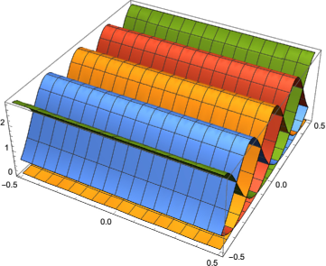
Figure 2.1: Squares of the absolute values of the wave functions on a quadratic torus for $M=4$.

We find it instructive to derive the quantization condition on $M$. Let us follow the discussion by [32]. Consider a $\mathrm{U}(1)$ gauge group in the torus with a magnetic flux given by the gauge potential

$$A(z+\zeta)=\frac{B}{2\operatorname{Im}\tau}\operatorname{Im}\bigl{(}(\bar{z}+\bar{\zeta})\mathop{}\!\mathrm{d}z\bigr{)}\;.$$ (2.3)

Then, if the wave function $\psi^{j,M}(z,\tau,\zeta)$ has charge $q$ under this $\mathrm{U}(1)$, its transformation under torus translations are

$$\psi^{j,M}(z+1,\tau,\zeta) =\exp\bigg{(}\frac{\hskip 0.43057pt\mathrm{i}\hskip 0.43057pt\,qB}{2\operatorname{Im}\tau}\operatorname{Im}(z+\zeta)\bigg{)}\,\psi^{j,M}(z,\tau,\zeta)\;,$$ (2.4a)

$$\psi^{j,M}(z+\tau,\tau,\zeta) =\exp\bigg{(}\frac{\hskip 0.43057pt\mathrm{i}\hskip 0.43057pt\,qB}{2\operatorname{Im}\tau}\operatorname{Im}(z+\zeta)\bar{\tau}\bigg{)}\,\psi^{j,M}(z,\tau,\zeta)\;.$$ (2.4b)

In order to have consistency through a contractible loop in the torus, we must get the same wave function shifting $z\rightarrow z+\tau+1$ as in the case where we shift by $z\rightarrow z+1+\tau$. Then,

$$\psi^{j,M}(z+\tau+1,\tau,\zeta)=\exp\bigg{(}\frac{\hskip 0.43057pt\mathrm{i}\hskip 0.43057pt\,qB}{2\operatorname{Im}\tau}\operatorname{Im}\bigl{(}(z+\zeta+1\bigr{)}\bar{\tau})\bigg{)}\psi^{j,M}(z+1,\tau,\zeta)$$

$$=\exp\bigg{(}\frac{\hskip 0.43057pt\mathrm{i}\hskip 0.43057pt\,qB}{2\operatorname{Im}\tau}\operatorname{Im}\bigl{(}(z+\zeta+1\bigr{)}\bar{\tau})\bigg{)}\exp\bigg{(}\frac{\hskip 0.43057pt\mathrm{i}\hskip 0.43057pt\,qB}{2\operatorname{Im}\tau}\operatorname{Im}(z+\zeta)\bigg{)}\psi^{j,M}(z,\tau,\zeta)$$

$$=\exp\bigg{(}\hskip 0.43057pt\mathrm{i}\hskip 0.43057pt\,\frac{qB\operatorname{Im}\bar{\tau}}{2\operatorname{Im}\tau}\bigg{)}\exp\bigg{(}\frac{\hskip 0.43057pt\mathrm{i}\hskip 0.43057pt\,qB}{2\operatorname{Im}\tau}\operatorname{Im}\bigl{(}\bar{\tau}(z+\zeta)\bigr{)}\bigg{)}\exp\bigg{(}\frac{\hskip 0.43057pt\mathrm{i}\hskip 0.43057pt\,qB}{2\operatorname{Im}\tau}\operatorname{Im}(z+\zeta)\bigg{)}\psi^{j,M}(z,\tau,\zeta)\mathrlap{\;,}$$ (2.5)

where we used first equation 2.4b and then equation 2.4a. On the other hand,

$$\psi^{j,M}(z+\tau+1,\tau,\zeta)=\exp\bigg{(}\frac{\hskip 0.43057pt\mathrm{i}\hskip 0.43057pt\,qB\operatorname{Im}(z+\zeta+\tau)}{2\operatorname{Im}\tau}\bigg{)}\psi^{j,M}(z+\tau,\tau,\zeta)$$

$$=\exp\bigg{(}\hskip 0.43057pt\mathrm{i}\hskip 0.43057pt\frac{qB\operatorname{Im}(z+\zeta+\tau)}{2\operatorname{Im}\tau}\bigg{)}\exp\bigg{(}\frac{\hskip 0.43057pt\mathrm{i}\hskip 0.43057pt\,qB}{2\operatorname{Im}\tau}\operatorname{Im}\bar{\tau}(z+\zeta)\bigg{)}\psi^{j,M}(z,\tau,\zeta)$$

$$=\exp\bigg{(}\hskip 0.43057pt\mathrm{i}\hskip 0.43057pt\frac{qB\operatorname{Im}\tau}{2\operatorname{Im}\tau}\bigg{)}\exp\bigg{(}\frac{\hskip 0.43057pt\mathrm{i}\hskip 0.43057pt\,qB}{2\operatorname{Im}\tau}\operatorname{Im}(\bar{\tau}(z+\zeta))\bigg{)}\exp\bigg{(}\frac{\hskip 0.43057pt\mathrm{i}\hskip 0.43057pt\,qB}{2\operatorname{Im}\tau}\operatorname{Im}(z+\zeta)\bigg{)}\psi^{j,M}(z,\tau,\zeta)\;,$$ (2.6)

where we used first equation 2.4a and then equation 2.4b. Imposing that equation 2.5 and equation 2.6 yield the same wave function leads to the flux quantization condition

$$qB=2\pi M\;,$$ (2.7)

with $M$ an arbitrary integer. Therefore, in what follows, we will not consider $q$ and $B$ individually, but only the integer $M$ instead. Then, we have

$$\psi^{j,M}(z+1,\tau,\zeta) =\exp\bigg{(}\frac{\hskip 0.43057pt\mathrm{i}\hskip 0.43057pt\,\pi M}{\operatorname{Im}\tau}\operatorname{Im}(z+\zeta)\bigg{)}\,\psi^{j,M}(z,\tau,\zeta)\;,$$ (2.8a)

$$\psi^{j,M}(z+\tau,\tau,\zeta) =\exp\bigg{(}\frac{\hskip 0.43057pt\mathrm{i}\hskip 0.43057pt\,\pi M}{\operatorname{Im}\tau}\operatorname{Im}(z+\zeta)\bar{\tau}\bigg{)}\,\psi^{j,M}(z,\tau,\zeta)\;.$$ (2.8b)

3 Yukawa couplings

3.1 Couplings from overlap integrals

One of the main rationales of working out the wave functions in section 2 is that the overlaps of wave functions yield the (Yukawa) couplings of the model. Let us consider a $4+2$ dimensional theory which is compactified on a torus $\mathbb{T}^{2}$. There is a gauge group breaking $\mathrm{U}(N)\rightarrow\mathrm{U}(N_{a})\times\mathrm{U}(N_{b})\times\mathrm{U}(N_{c})$ with $N=N_{a}+N_{b}+N_{c}$ due to the introduction of a magnetic flux in the compact dimensions given by

$$F_{z\bar{z}}=\frac{\pi\hskip 0.43057pt\mathrm{i}\hskip 0.43057pt}{\text{Im}\tau}\begin{pmatrix}\frac{m_{a}}{N_{a}}\mathds{1}_{N_{a}\times N_{a}}&0&0\\ 0&\frac{m_{b}}{N_{b}}\mathds{1}_{N_{b}\times N_{b}}&0\\ 0&0&\frac{m_{c}}{N_{c}}\mathds{1}_{N_{c}\times N_{c}}\end{pmatrix}\;,$$ (3.1)

where we will assume that $s_{\alpha}=\frac{m_{\alpha}}{N_{\alpha}}$ is an integer for $\alpha\in\{a,b,c\}$. Then, in [32, equation (5.7)] one finds that Yukawa couplings of the 4D effective theory are given by

$$Y_{ijk}(\widetilde{\zeta},\tau)=g\,\sigma_{abc}\,\int\limits_{\mathds{T}^{2}}\!\mathop{}\!\mathrm{d}^{2}z\,\psi^{i,\mathcal{I}_{ab}}(z,\tau,\zeta_{ab})\,\psi^{j,\mathcal{I}_{ca}}(z,\tau,\zeta_{ca})\,\left(\psi^{k,\mathcal{I}_{cb}}(z,\tau,\zeta_{cb})\right)^{*}\;.$$ (3.2)

Here, $\psi^{i,\mathcal{I}_{ab}}(z,\tau,\zeta_{ab})$ are the wave functions of equation 2.1 that represent chiral fermions bifundamentals transforming as $(\boldsymbol{N}_{a},\overline{\boldsymbol{N}}_{b})$ under $\mathrm{U}(N_{a})\times\mathrm{U}(N_{b})$, and similarly for $\psi^{j,\mathcal{I}_{ca}}$ and $\psi^{k,\mathcal{I}_{cb}}$. The multiplicities of $\mathcal{I}_{\alpha\beta}$ of these bifundamentals are given by

$$\mathcal{I}_{\alpha\beta}=s_{\alpha}-s_{\beta}\;,$$ (3.3)

which implies that

$$\mathcal{I}_{ab}+\mathcal{I}_{bc}+\mathcal{I}_{ca}=0\;.$$ (3.4)

Furthermore, $g$ is the $(4+2)$–dimensional gauge coupling, and $\sigma_{abc}=\operatorname{sign}(\mathcal{I}_{ab}\mathcal{I}_{bc}\mathcal{I}_{ca})$  [32] is a sign which is equal to $-1$ throughout our discussion. The $\zeta_{\alpha\beta}$ are given by

$$\zeta_{\alpha\beta}=\frac{s_{\alpha}\zeta_{\alpha}-s_{\beta}\zeta_{\beta}}{s_{\alpha}-s_{\beta}}$$ (3.5)

for $\alpha,\beta\in\{a,b,c\}$. Finally, $\zeta_{\alpha}$ are the Abelian Wilson lines associated to the group $\mathrm{U}(N_{\alpha})$ for $\alpha\in\{a,b,c\}$. $\zeta_{cb}$ and $\zeta_{ca}$ are defined similarly. As one can see from equation 2.1, the $\zeta_{\alpha}$ represent translation of the torus origin. However, as shown in [32] if all three wave functions are shifted by the same Wilson line, then the values of the Yukawa couplings are unaffected.

3.2 Yukawa couplings for generic flux parameters

Let us now discuss how one can reduce the overlap integrals (3.2) to a linear combination of $\vartheta$–functions. We follow the strategy of [32], but generalize the result to the cases $\mathcal{I}_{ab}>1$ and/or $\gcd(\mathcal{I}_{ab},\mathcal{I}_{ca},\mathcal{I}_{bc})>1$, with $\mathcal{I}_{ab},\mathcal{I}_{ca}>0$ and $\mathcal{I}_{bc}<0$. Note that the analogous discussion applies to the case in which $\mathcal{I}_{ab}$ and $\mathcal{I}_{ca}$ are negative [32, cf. the discussion around equation (5.6)].

In order to find closed–form expressions for the Yukawa couplings, one uses two important facts [32]:

1. products of $\vartheta$–functions can be expanded in terms of $\vartheta$–functions, see [32, equation (5.8)], and that

2. the $\vartheta$–functions fulfill certain orthogonality and completeness relations.

These facts allow one to find analytic expressions for the Yukawa couplings (3.2) that do no longer involve integrals [32]. In more detail, starting from (3.2), one obtains (cf. [32, equation (5.15)])

$$Y_{ijk}(\widetilde{\zeta},\tau) =\mathcal{N}_{abc}\,\mathrm{e}^{\frac{H(\widetilde{\zeta},\tau)}{2}}\,\sum\limits_{m\in\mathds{Z}_{\mathcal{I}_{bc}}}\delta_{k,i+j+\mathcal{I}_{ab}\,m}\,\vartheta\begin{bmatrix}\frac{\mathcal{I}_{ca}i-\mathcal{I}_{ab}j+\mathcal{I}_{ab}\mathcal{I}_{ca}m}{-\mathcal{I}_{ab}\mathcal{I}_{bc}\mathcal{I}_{ca}}\\ 0\end{bmatrix}\bigl{(}\widetilde{\zeta},\tau\,|\mathcal{I}_{ab}\mathcal{I}_{bc}\mathcal{I}_{ca}|\bigr{)}\;,$$ (3.6)

where

$$\mathcal{N}_{abc}=g\,\sigma_{abc}\,\left(\frac{2\operatorname{Im}\tau}{\mathcal{A}^{2}}\right)^{1/4}\,\left|\frac{\mathcal{I}_{ab}\mathcal{I}_{ca}}{\mathcal{I}_{bc}}\right|^{1/4}$$ (3.7)

is a normalization constant and the Wilson line dependence is encoded in the quantities

$$\widetilde{\zeta} :=-\mathcal{I}_{ab}\,\mathcal{I}_{ca}\,(\zeta_{ca}-\zeta_{ab})=d^{\alpha\beta\gamma}\,s_{\alpha}\,\zeta_{\alpha}\,\mathcal{I}_{\beta\gamma}$$ (3.8)

and

$$\frac{H(\widetilde{\zeta},\tau)}{2} :=\frac{\pi\hskip 0.43057pt\mathrm{i}\hskip 0.43057pt}{\operatorname{Im}\tau}\left(\mathcal{I}_{ab}\,\zeta_{ab}\,\operatorname{Im}\zeta_{ab}+\mathcal{I}_{bc}\,\zeta_{bc}\,\operatorname{Im}\zeta_{bc}+\mathcal{I}_{ca}\,\zeta_{ca}\,\operatorname{Im}\zeta_{ca}\right)$$

$$=\frac{\pi\hskip 0.43057pt\mathrm{i}\hskip 0.43057pt}{\operatorname{Im}\tau}\left|\mathcal{I}_{ab}\,\mathcal{I}_{bc}\,\mathcal{I}_{ab}\right|^{-1}\frac{\widetilde{\zeta}\,\operatorname{Im}\widetilde{\zeta}}{\operatorname{Im}\tau}\;.$$ (3.9)

with

$$d^{\alpha\beta\gamma}=\begin{cases}1\;,&\text{if $\{\alpha,\beta,\gamma\}$ is an even permutation of $\{1,2,3\}$}\;,\\ 0\;,&\text{otherwise}\;,\end{cases}$$ (3.10)

where we have used [32, equation (5.28)]. Cremades et al. obtain then [32, equation (5.15)]

$$Y_{ijk}(\widetilde{\zeta},\tau) =\mathcal{N}_{abc}\mathrm{e}^{\frac{H(\widetilde{\zeta},\tau)}{2}}\,\vartheta\begin{bmatrix}-\left(\frac{j}{\mathcal{I}_{ca}}+\frac{k}{\mathcal{I}_{bc}}\right)/\mathcal{I}_{ab}\\ 0\end{bmatrix}\bigl{(}\widetilde{\zeta},\tau\,|\mathcal{I}_{ab}\mathcal{I}_{bc}\mathcal{I}_{ca}|\bigr{)}\qquad\text{for }i=k-j\mod\mathcal{I}_{ab}\;.$$ (3.11)

This expression yields the correct couplings only if $\mathcal{I}_{ab}=1$, which implies that $d=1$, where

$$d:=\gcd\bigl{(}|\mathcal{I}_{ab}|,|\mathcal{I}_{ca}|,|\mathcal{I}_{bc}|\bigr{)}\;.$$ (3.12)

To see that we need to demand that $d=1$ for (3.11) to hold, notice that in (3.6) the integers $i$, $j$ and $k$ are only defined modulo $\mathcal{I}_{ab}$, $\mathcal{I}_{bc}$ and $\mathcal{I}_{ca}$, respectively. This is evident from the overlap integral (3.2), where e.g. $\psi^{i,\mathcal{I}_{ab}}(z,\tau,\zeta_{ab})=\psi^{i+\mathcal{I}_{ab},\mathcal{I}_{ab}}(z,\tau,\zeta_{ab})$. However, if $\gcd(|\mathcal{I}_{ab}|,|\mathcal{I}_{ca}|)>1$ or $|\mathcal{I}_{ab}|>1$, shifting $i$ (or $j$) by $|\mathcal{I}_{ab}|$ (or $(|\mathcal{I}_{ca}|$), which leaves the wave functions invariant and hence has to produce the same overlap integral, leads to different results for the Yukawa couplings when using (3.11).

To obtain the general expression, let us look at [37, Proposition II.6.4. on p. 221]

$$\vartheta\begin{bmatrix}\!\frac{j}{\mathcal{I}_{ab}}\!\\[1.29167pt] \!0\!\end{bmatrix}(z_{1},\mathcal{I}_{ab}\tau)\cdot\vartheta\begin{bmatrix}\!\frac{j}{\mathcal{I}_{ca}}\!\\[1.29167pt] \!0\!\end{bmatrix}(z_{2},\mathcal{I}_{ca}\tau)=\sum\limits_{\mathclap{m\in\mathds{Z}_{\mathcal{I}_{ab}+\mathcal{I}_{ca}}}}\vartheta\begin{bmatrix}\frac{i+j+\mathcal{I}_{ab}m}{\mathcal{I}_{ab}+\mathcal{I}_{ca}}\\ 0\end{bmatrix}\bigl{(}z_{1}+z_{2},(\mathcal{I}_{ab}+\mathcal{I}_{ca})\tau\bigr{)}\\ \vartheta\begin{bmatrix}\frac{\mathcal{I}_{ca}i-\mathcal{I}_{ab}j+\mathcal{I}_{ab}\mathcal{I}_{ca}\,m}{\mathcal{I}_{ab}\mathcal{I}_{ca}(\mathcal{I}_{ab}+\mathcal{I}_{ca})}\\ 0\end{bmatrix}\left(\mathcal{I}_{ca}\,z_{1}-\mathcal{I}_{ab}\,z_{2},\mathcal{I}_{ab}\mathcal{I}_{ca}(\mathcal{I}_{ab}+\mathcal{I}_{ca})\tau\right)\;,$$ (3.13)

which was used in [32]. In our wave functions, $z_{1}=\mathcal{I}_{ab}\,(z+\zeta_{ab})$ and $z_{2}=\mathcal{I}_{ca}\,(z+\zeta_{ca})$, so that in the overlap integral $z_{1}+z_{2}=\mathcal{I}_{cb}\,(z+\zeta_{cb})$ and $\mathcal{I}_{ca}\,z_{1}-\mathcal{I}_{ab}\,z_{2}=\widetilde{\zeta}$. One thus obtains (cf. [32, equation (5.12)])

$$\psi^{i,\mathcal{I}_{ab}}(z,\tau,\zeta_{ab})\cdot\psi^{j,\mathcal{I}_{ca}}(z,\tau,\zeta_{ca})=\mathcal{A}^{-1/2}\,(2\operatorname{Im}\tau)^{1/4}\,\left|\frac{\mathcal{I}_{ab}\,\mathcal{I}_{ca}}{\mathcal{I}_{bc}}\right|^{1/4}\mathrm{e}^{\frac{H(\widetilde{\zeta},\tau)}{2}}\\ \sum\limits_{\mathclap{m\in\mathds{Z}_{|\mathcal{I}_{bc}|}}}\psi^{i+j+\mathcal{I}_{ab}\,m,\mathcal{I}_{cb}}(z,\tau,\mathcal{I}_{cb})\,\vartheta\begin{bmatrix}\frac{\mathcal{I}_{ca}i-\mathcal{I}_{ab}j+\mathcal{I}_{ab}\mathcal{I}_{ca}\,m}{\mathcal{I}_{ab}\mathcal{I}_{ca}(\mathcal{I}_{ab}+\mathcal{I}_{ca})}\\ 0\end{bmatrix}\left(\widetilde{\zeta},\mathcal{I}_{ab}\mathcal{I}_{ca}(\mathcal{I}_{ab}+\mathcal{I}_{ca})\tau\right)\;.$$ (3.14)

The product (3.14) gets projected on a third wave function $\psi^{k,\mathcal{I}_{ab}+\mathcal{I}_{ca}}$ via the overlap integral (3.2). This means that $k$ has to “match”, i.e. $m$ has to be a solution of the congruence equation

$$\mathcal{I}_{ab}\,m+i+j=k\mod\mathcal{I}_{bc}\;.$$ (3.15)

Now observe that, since $\mathcal{I}_{ab}+\mathcal{I}_{bc}+\mathcal{I}_{ca}=0$, $\gcd\bigl{(}|\mathcal{I}_{ab}|,|\mathcal{I}_{cb}|\bigr{)}=d$ with $d$ from equation 3.12. Equation 3.15 is a linear congruence equation for the variable $m$. It is known that (cf. e.g. [38, Lemma 3 on p. 37]) if

$$k-i-j=0\mod d\,,$$ (3.16)

the linear congruence of equation 3.15 has $d$ solutions. Otherwise there is no solution. Note that the condition (3.16) provides us with a selection rule for the Yukawa couplings, which can be interpreted as a $\mathds{Z}_{d}$ flavor symmetry (cf. [39]). We thus know that the Yukawa couplings will be proportional to

$$\Delta_{i+j,k}^{(d)}:=\begin{dcases}1\;,&\text{if }i+j=k\mod d\;,\\ 0\;,&\text{otherwise}\;.\end{dcases}$$ (3.17)

Consider now combinations of $i$, $j$ and $k$ satisfying the selection rule (3.16). This means that

$$k-i-j=m^{\prime}\,d$$ (3.18)

with some integer $m^{\prime}=(k-i-j)/d$. Define now $\mathcal{I}_{ab}^{\prime}=\mathcal{I}_{ab}/d$, $\mathcal{I}_{ca}^{\prime}=\mathcal{I}_{ca}/d$ and $\mathcal{I}_{bc}^{\prime}=\mathcal{I}_{bc}/d$, which are integers because of equation 3.12. We can thus divide equation 3.15 by $d$ to get

$$|\mathcal{I}_{ab}^{\prime}|\,m=m^{\prime}\mod|\mathcal{I}_{bc}^{\prime}|\;,$$ (3.19)

where $\gcd\bigl{(}|\mathcal{I}_{ab}^{\prime}|,|\mathcal{I}_{bc}^{\prime}|\bigr{)}=1$. Equation 3.19 can be solved with e.g. the Mathematica command FindInstance. However, as we shall discuss now, one can find a closed–form expression for the solution. The linear congruence (3.19) has one (inequivalent) solution $m=m_{0}$, which is given by $\bigl{[}|\mathcal{I}_{ab}^{\prime}|\bigr{]}_{(|\mathcal{I}_{bc}^{\prime}|)}m^{\prime}$ where $\bigl{[}|\mathcal{I}_{ab}^{\prime}|\bigr{]}_{(|\mathcal{I}_{bc}^{\prime}|)}$ is the multiplicative inverse of $|\mathcal{I}_{ab}^{\prime}|$ modulo $|\mathcal{I}_{bc}^{\prime}|$. According to Euler’s theorem (cf. e.g. [38, Theorem 1 on p. 64]), the multiplicative inverse can be expressed via the Euler $\phi$–function, $\bigl{[}|\mathcal{I}_{ab}^{\prime}|\bigr{]}_{(|\mathcal{I}_{bc}^{\prime}|)}=(\mathcal{I}_{ab}^{\prime})^{\phi\bigl{(}|\mathcal{I}_{bc}^{\prime}|\bigr{)}-1}$. This means that

$$m_{0}=(\mathcal{I}_{ab}^{\prime})^{\phi\bigl{(}|\mathcal{I}_{bc}^{\prime}|\bigr{)}-1}\,\frac{k-i-j}{d}\mod|\mathcal{I}_{bc}^{\prime}|\;.$$ (3.20)

Note that the Euler $\phi$–function is implemented in Mathematica as EulerPhi. Relation (3.20) implies that one particular solution $m_{0}$ of equation 3.15 satisfies

$$\mathcal{I}_{ab}\,m_{0}=(\mathcal{I}_{ab}^{\prime})^{\phi\bigl{(}|\mathcal{I}_{bc}^{\prime}|\bigr{)}}\,(k-i-j)\mod|\mathcal{I}_{bc}|\;.$$ (3.21)

Given the solution $m_{0}$ in equation 3.20, the $d$ solutions of equation 3.15 are given by

$$m=m_{0}-|\mathcal{I}_{bc}^{\prime}|\,t\quad\text{for }t=0,\dots,(d-1)\;.$$ (3.22)

Thus, using equation 3.22 in (3.6), we see that the Yukawa couplings are given by

$$Y_{ijk}(\widetilde{\zeta},\tau) =\mathcal{N}_{abc}\mathrm{e}^{\frac{H(\widetilde{\zeta},\tau)}{2}}\,\Delta_{i+j,k}^{(d)}\,\sum_{t=0}^{d-1}\vartheta\begin{bmatrix}\frac{\mathcal{I}_{ca}i-\mathcal{I}_{ab}j+\mathcal{I}_{ab}\mathcal{I}_{ca}m_{0}}{|\mathcal{I}_{ab}\mathcal{I}_{bc}\mathcal{I}_{ca}|}+\frac{t}{d}\\ 0\end{bmatrix}\left(\widetilde{\zeta},|\mathcal{I}_{ab}\mathcal{I}_{ca}\mathcal{I}_{bc}|\tau\right)\;,$$ (3.23)

Equation 3.23 can be simplified further. Let us define

$$P :=|\mathcal{I}_{ab}\mathcal{I}_{ca}\mathcal{I}_{bc}|\;,$$ (3.24a)

$$\lambda :=\operatorname{lcm}\bigl{(}|\mathcal{I}_{ab}|,|\mathcal{I}_{ca}|,|\mathcal{I}_{bc}|\bigr{)}\;.$$ (3.24b)

Next we note that

$$P=\lambda\,d^{2}\;.$$ (3.25)

Then equation 3.23 can be recast as

$$Y_{ijk}(\widetilde{\zeta},\tau)=\mathcal{N}_{abc}\mathrm{e}^{\frac{H(\widetilde{\zeta},\tau)}{2}}\,\sum_{t=0}^{d-1}\vartheta\begin{bmatrix}\frac{1}{d}\left(\frac{\widehat{\alpha}_{ijk}}{\lambda}+t\right)\\ 0\end{bmatrix}\left(\widetilde{\zeta},P\tau\right)\;,$$ (3.26)

where

$$\widehat{\alpha}_{ijk}=\mathcal{I}_{ca}^{\prime}\,i-\mathcal{I}_{ab}^{\prime}\,j+\mathcal{I}_{ca}^{\prime}\,\mathcal{I}_{ab}\,m_{0}$$ (3.27)

is an integer. Using equation 3.20, $\widehat{\alpha}_{ijk}$ becomes

$$\widehat{\alpha}_{ijk}=\mathcal{I}_{ca}^{\prime}\,i-\mathcal{I}_{ab}^{\prime}\,j+\mathcal{I}_{ca}^{\prime}\,(\mathcal{I}_{ab}^{\prime})^{\phi\bigl{(}|\mathcal{I}_{bc}^{\prime}|\bigr{)}}\,(k-i-j)\mod\lambda\,d\;.$$ (3.28)

Now we can use equation A.4 to express the sum (3.26) as

$$Y_{ijk}(\widetilde{\zeta},\tau) =\mathcal{N}_{abc}\mathrm{e}^{\frac{H(\widetilde{\zeta},\tau)}{2}}\,\sum_{t=0}^{d-1}\sum_{\ell=-\infty}^{\infty}\exp\left[\hskip 0.43057pt\mathrm{i}\hskip 0.43057pt\pi\left(\frac{1}{d}\frac{\widehat{\alpha}_{ijk}}{\lambda}+\frac{1}{d}t+\ell\right)^{2}P\,\tau\right]\,\exp\left[2\pi\hskip 0.43057pt\mathrm{i}\hskip 0.43057pt\,\left(\frac{\widehat{\alpha}_{ijk}}{\lambda\,d}+\frac{t}{d}+\ell\right)\,\widetilde{\zeta}\right]$$

$$=\mathcal{N}_{abc}\mathrm{e}^{\frac{H(\widetilde{\zeta},\tau)}{2}}\,\sum_{\ell=-\infty}^{\infty}\sum_{t=0}^{d-1}\exp\left[\hskip 0.43057pt\mathrm{i}\hskip 0.43057pt\pi\left(\frac{\widehat{\alpha}_{ijk}}{\lambda}+t+d\,\ell\right)^{2}\lambda\,\tau\right]\,\exp\left[2\pi\hskip 0.43057pt\mathrm{i}\hskip 0.43057pt\,\left(\frac{\widehat{\alpha}_{ijk}}{\lambda}+t+\ell d\right)\,\frac{\widetilde{\zeta}}{d}\right]$$

$$=\mathcal{N}_{abc}\mathrm{e}^{\frac{H(\widetilde{\zeta},\tau)}{2}}\,\sum_{\ell^{\prime}=-\infty}^{\infty}\exp\left[\hskip 0.43057pt\mathrm{i}\hskip 0.43057pt\pi\left(\frac{\widehat{\alpha}_{ijk}}{\lambda}+\ell^{\prime}\right)^{2}\lambda\,\tau\right]\,\exp\left[2\pi\hskip 0.43057pt\mathrm{i}\hskip 0.43057pt\,\left(\frac{\widehat{\alpha}_{ijk}}{\lambda\,d}+\ell^{\prime}\right)\,\frac{\widetilde{\zeta}}{d}\right]$$

$$=\mathcal{N}_{abc}\mathrm{e}^{\frac{H(\widetilde{\zeta},\tau)}{2}}\,\vartheta\begin{bmatrix}\frac{\widehat{\alpha}_{ijk}}{\lambda}\\ 0\end{bmatrix}\left(\frac{\widetilde{\zeta}}{d},\lambda\,\tau\right)\;.$$ (3.29)

Here, $\ell^{\prime}=d\,\ell+t$. When $\ell$ runs over all integers, and $t$ runs from $0$ to $d-1$, $\ell^{\prime}$ runs over all integers. The $\widehat{\alpha}_{ijk}$ are integers. Therefore, the physical Yukawa couplings are given by

$$Y_{ijk}(\widetilde{\zeta},\tau) =\mathcal{N}_{abc}\,\mathrm{e}^{\frac{H(\widetilde{\zeta},\tau)}{2}}\,\Delta_{i+j,k}^{(d)}\,\vartheta\begin{bmatrix}\frac{\mathcal{I}_{ca}^{\prime}\,i-\mathcal{I}_{ab}^{\prime}\,j+\mathcal{I}_{ca}^{\prime}\,\left(\mathcal{I}_{ab}^{\prime}\right)^{\phi\left(|\mathcal{I}_{bc}^{\prime}|\right)}\,(k-i-j)}{\lambda}\\ 0\end{bmatrix}\left(\frac{\widetilde{\zeta}}{d},\lambda\,\tau\right)$$ (3.30)

with $d$ from equation 3.12, $\Delta_{i+j,k}^{(d)}$ from equation 3.17, $\lambda$ from equation 3.24b and assuming $\mathcal{I}_{ab},\,\mathcal{I}_{ca}>0$ and $\mathcal{I}_{bc}<0$. Note that if $d=1$ and $\mathcal{I}_{ab}=1$, this formula reproduces equation 3.11. Further, a priori this expression does not rely on supersymmetry, it is simply derived from the overlap of wave functions. However, one may expect the scalar wave function to be subject to substantial corrections in non–supersymmetric theories. In section 5 we will argue that magnetized tori may not comply with these expectations, and that this formula may even be a good leading–order result in a non–supersymmetric theory. The normalization factors in equation 3.30 are

$$\mathcal{N}_{abc}=g\,\sigma_{abc}\,\bigg{(}\frac{2\operatorname{Im}\tau}{\mathcal{A}^{2}}\bigg{)}^{\nicefrac{{1}}{{4}}}\,\lambda^{\nicefrac{{1}}{{4}}}\,\left|\frac{1}{\mathcal{I}_{bc}^{\prime}}\right|^{\nicefrac{{1}}{{2}}}$$ (3.31)

with $g$ being the gauge coupling. In equation 4.39 we will express the normalization in terms of Kähler potential terms. Notice that if there are nontrivial relative Wilson lines, the normalization of the fields changes compared to the case without Wilson lines [32, equation (7.37)]. This has to be taken into account when computing physical Yukawa couplings. In what follows, we will set the Wilson lines to zero, leaving the detailed study of their impact on the modular flavor symmetries for future work. As mentioned above, the selection rule (3.16) entails a $\mathds{Z}_{d}$ symmetry. As we discuss in more detail in appendix D, out of a priori $P=\lambda\,d^{2}$ entries, at most $\nicefrac{{\lambda}}{{2}}+1$ are distinct.

4 Modular transformations

4.1 Modular groups and modular forms

The modular group $\Gamma=\mathrm{SL}(2,\mathds{Z})$ can be defined by the presentation relations

$$S^{4}=(S\,T)^{3}=\mathds{1}\quad\text{and}\quad S^{2}\,T=T\,S^{2}\;,$$ (4.1)

where the generators $S$ and $T$ are usually chosen as

$$S=\begin{pmatrix}0&1\\ -1&0\end{pmatrix}\quad\text{and}\quad T=\begin{pmatrix}1&1\\ 0&1\end{pmatrix}\;.$$ (4.2)

These generators act on the modulus $\tau$ according to

$$\tau\xmapsto{~{}S~{}}-\frac{1}{\tau}\quad\text{and}\quad\tau\xmapsto{~{}T~{}}\tau+1\;.$$ (4.3)

Hence, a general modular transformation acts on the modulus $\tau$ as

$$\tau~{}\xmapsto{~{}\gamma~{}}~{}\frac{a\,\tau+b}{c\,\tau+d}~{}=:~{}\gamma\,\tau\;,\quad\text{where}\quad\gamma~{}=\begin{pmatrix}a&b\\ c&d\end{pmatrix}\in\Gamma\;,$$ (4.4)

such that $ad-bc=1$ and $a,b,c,d\in\mathds{Z}$. Consequently, functions of $\tau$ also transform under $\gamma$. This is particularly true for modular forms, which are holomorphic functions of $\tau$ (also at $\tau\to\hskip 0.43057pt\mathrm{i}\hskip 0.43057pt\infty$) with $\operatorname{Im}\tau>0$ [40]. Modular forms $f_{\widehat{\alpha}}(\tau)$ of modular weight $k\in\mathds{N}$ and level $N=2,3,4,\ldots$ build finite vector spaces and transform under a modular transformation $\gamma\in\Gamma$ as [9]

$$f_{\widehat{\alpha}}(\tau)~{}\xmapsto{~{}\gamma~{}}~{}f_{\widehat{\alpha}}(\gamma\,\tau)~{}:=~{}(c\,\tau+d)^{k}\,\rho_{\boldsymbol{r}}(\gamma)_{\widehat{\alpha}\widehat{\beta}}\,f_{\widehat{\beta}}(\tau)\,,$$ (4.5)

where $\widehat{\alpha},\widehat{\beta}$ are considered here just as (integer) counters, $(c\,\tau+d)^{k}$ often gets referred to as automorphy factor, and $\rho_{\boldsymbol{r}}(\gamma)$ denotes an $r$-dimensional (irreducible) representation matrix of $\gamma$ under the finite modular group $\Gamma^{\prime}_{N}\cong\mathrm{SL}(2,\mathds{Z}_{N})$. These finite groups are defined by the relations

$$S^{4}=(S\,T)^{3}=\mathds{1}\,,\quad S^{2}\,T=T\,S^{2}\,,\quad T^{N}=\mathds{1}$$ (4.6)

and an additional relation that ensures finiteness for $N>5$.

It has been proposed in [1] that Yukawa couplings in quantum field theories can be modular forms, whereas, despite not being modular forms, “matter” superfields $\phi^{i}$ transform under a general modular transformation $\gamma\in\Gamma$ as

$$\phi^{i}~{}\xmapsto{~{}\gamma~{}}~{}(c\,\tau+d)^{k_{\phi}}\,\rho_{\boldsymbol{s}}(\gamma)_{ij}\,\phi^{j}\;.$$ (4.7)

Here $\rho_{\boldsymbol{s}}(\gamma)$ is the $s$-dimensional (reducible or irreducible) $\Gamma^{\prime}_{N}$ representation matrix. As for modular forms, the powers $k_{\phi}$ are also known as modular weights and are identical for the fields in the transformation. Thus, matter fields build a representation of the finite modular group $\Gamma^{\prime}_{N}$, which can be adopted as a symmetry of the underlying (quantum) field theory. In this scenario, $\Gamma^{\prime}_{N}$ can be considered a “modular flavor symmetry”.

In string–derived models, it is known that matter fields are subject to modular transformations similar to equation 4.7. Moreover, Yukawa couplings also transform as in equation 4.5. However, as we shall see in this section, the modular weights can be fractional and, hence, the emerging modular flavor symmetry is not necessarily one of the $\Gamma^{\prime}_{N}$. Yet, to obtain fractional modular weights it is not necessary to go all the way to strings, they already emerge from simpler settings such as magnetized tori (see e.g. [18, 19, 20, 21, 26, 27, 28, 30]). As we discuss in detail in detail in section 4.2, this follows already from the $\tau$–dependence of the normalization of the wave functions [32].

As a first step, let us review the modular symmetries associated with modular forms with half–integral modular weights [15]. In this case, one must consider instead of $\mathrm{SL}(2,\mathds{Z})$ its double cover, the so–called metaplectic group $\widetilde{\Gamma}=\mathrm{Mp}(2,\mathds{Z})$. The generators $\widetilde{S}$ and $\widetilde{T}$ of $\widetilde{\Gamma}$ satisfy the presentation

$$\widetilde{S}^{8}=(\widetilde{S}\,\widetilde{T})^{3}=\mathds{1}\quad\text{and}\quad\widetilde{S}^{2}\widetilde{T}=\widetilde{T}\,\widetilde{S}^{2}\;,$$ (4.8)

which are represented by the choice

$$\widetilde{S}=(S,-\sqrt{-\tau})\quad\text{and}\quad\widetilde{T}=(T,+1)\;,\qquad S,T\in\Gamma\;.$$ (4.9)

In terms of these, the elements of the metaplectic group are given by

$$\widetilde{\Gamma}=\left\{\widetilde{\gamma}=(\gamma,\varphi(\gamma,\tau))~{}|~{}\gamma\in\Gamma,\ \varphi(\gamma,\tau)=\pm(c\,\tau+d)^{\nicefrac{{1}}{{2}}}\right\}\;,$$ (4.10)

subject to the multiplication rule

$$\left(\gamma_{1},\,\varphi(\gamma_{1},\tau)\right)\left(\gamma_{2},\,\varphi(\gamma_{2},\tau)\right)=\left(\gamma_{1}\gamma_{2},\,\varphi(\gamma_{1},\gamma_{2}\,\tau)\varphi(\gamma_{2},\tau)\right)\;.$$ (4.11)

To determine the sign of $\varphi(\gamma,\tau)$ for an arbitrary element $\widetilde{\gamma}\in\widetilde{\Gamma}$, one has to express $\widetilde{\gamma}$ as a product of the metaplectic generators (4.9) and then use the multiplication rule (4.11).

The modular transformations $\widetilde{\gamma}$ act on the modulus still just as $\gamma$, according to equation 4.4. In contrast, modular forms of modular weight $\nicefrac{{k}}{{2}}$ and level $4N$, where $k,N\in\mathds{N}$, transform as

$$f_{\widehat{\alpha}}(\tau)~{}\xmapsto{~{}\widetilde{\gamma}~{}}~{}f_{\widehat{\alpha}}(\widetilde{\gamma}\,\tau)~{}:=~{}\varphi(\gamma,\tau)^{k}\,\rho_{\boldsymbol{r}}(\widetilde{\gamma})_{\widehat{\alpha}\widehat{\beta}}\,f_{\widehat{\beta}}(\tau)\;.$$ (4.12)

Here $\varphi(\gamma,\tau)^{k}$ is now the automorphy factor, and $\rho_{\boldsymbol{r}}(\widetilde{\gamma})$ is an (irreducible) representation matrix of $\widetilde{\gamma}$ in the finite metaplectic modular group $\widetilde{\Gamma}_{4N}$. The generators $\widetilde{S}$ and $\widetilde{T}$ of this discrete group satisfy

$$\widetilde{S}^{8}=(\widetilde{S}\,\widetilde{T})^{3}=\mathds{1}\;,\quad\widetilde{S}^{2}\widetilde{T}=\widetilde{T}\,\widetilde{S}^{2}\;,\quad\widetilde{T}^{4N}=\mathds{1}$$ (4.13)

and, for $N>1$, a relation to ensure the finiteness of the group. This amounts to finding appropriate combinations of $\widetilde{S}$ and $\widetilde{T}$ that yield $\mathds{1}_{2}\mod 4N$, where the modulo condition is to be understood componentwise, and then demand that this combination yields identity in the finite group. For $N=2$ we adopt the choice by [15, equation (21)]

$$\widetilde{S}^{5}\widetilde{T}^{6}\widetilde{S}\widetilde{T}^{4}\widetilde{S}\widetilde{T}^{2}\widetilde{S}\widetilde{T}^{4}=\mathds{1}\;,$$ (4.14)

and for $N=3$ we choose

$$\widetilde{S}\widetilde{T}^{3}\widetilde{S}\widetilde{T}^{-2}\widetilde{S}^{-1}\widetilde{T}\widetilde{S}\widetilde{T}^{-3}\widetilde{S}^{-1}\widetilde{T}^{2}\widetilde{S}^{-1}\widetilde{T}^{-1}=\mathds{1}\;.$$ (4.15)

Note that $\widetilde{\Gamma}_{4N}$ is the double cover of $\Gamma^{\prime}_{4N}$. It is known that $\widetilde{\Gamma}_{4}\cong[96,67]$, $\widetilde{\Gamma}_{8}\cong[768,1085324]$ and $\widetilde{\Gamma}_{12}$ is a group of order 2304. We use here the unique identifiers assigned by the computer program GAP [41]. For example, $[96,67]$ denotes a finite discrete group of order 96, where 67 labels the group.

Finally, in field theories endowed with $\widetilde{\Gamma}_{4N}$ symmetries, the modular transformations of matter fields are given by

$$\phi^{i}~{}\xmapsto{~{}\widetilde{\gamma}~{}}~{}\varphi(\gamma,\tau)^{k_{\phi}}\,\rho_{\boldsymbol{s}}(\widetilde{\gamma})_{ij}\,\phi^{j}\;,$$ (4.16)

where $\rho_{\boldsymbol{s}}(\widetilde{\gamma})$ is now a (reducible or irreducible) $\widetilde{\Gamma}_{4N}$ representation. As we shall see, this behavior is natural in toroidal compactifications with magnetic fluxes.

4.2 Normalization of the wave functions and modular weights

The wave functions in equation 2.1 satisfy

$$\int\limits_{\mathds{T}^{2}}\!\mathop{}\!\mathrm{d}^{2}z\,|\psi^{j,M}(z,\tau,\zeta)|^{2}=\mathcal{A}\,\int\limits_{0}^{1}\!\mathop{}\!\mathrm{d}x\,\int\limits_{0}^{1}\!\mathop{}\!\mathrm{d}y\,|\psi^{j,M}(x+\tau\,y,\tau,\zeta)|^{2}\overset{!}{=}1\;,$$ (4.17)

where $\mathds{T}^{2}$ denotes the fundamental domain of the torus, cf. appendix B. The normalization constant $\mathcal{N}\propto(\operatorname{Im}\tau)^{-\nicefrac{{1}}{{4}}}$ in equation 2.2 is chosen in such a way that the normalization condition (4.17) holds. This implies, in particular, that the Kähler metric is proportional to $(\operatorname{Im}\tau)^{-\nicefrac{{1}}{{2}}}$, i.e.

$$K_{i\bar{\imath}}\propto\frac{1}{\left(\operatorname{Im}\tau\right)^{\nicefrac{{1}}{{2}}}}\;,$$ (4.18)

i.e. the modular weight of the 4D fields $\phi^{j,M}$ describing the zero modes is $k_{\phi}=-\nicefrac{{1}}{{2}}$. We survey the modular weights of the fields, coupling and superpotential in table 4.1.

object	$\psi^{j,M}$	$\phi^{j,M}$	$\Omega^{j,M}$	$Y_{ijk}$	$\mathscr{W}$
modular weight $k$	$\nicefrac{{1}}{{2}}$	$-\nicefrac{{1}}{{2}}$	$0$	$\nicefrac{{1}}{{2}}$	$-1$

Table 4.1: Modular weights of the $\mathds{T}^{2}$ wave functions $\psi^{j,M}$, 4D fields $\phi^{j,M}$, 6D fields $\Omega^{j,M}$, Yukawa couplings $Y_{ijk}$, and superpotential $\mathscr{W}$.

The modular weights $k_{\psi}$ of the wave functions can be inferred from their normalization factor $\mathcal{N}$ in equation 2.2 to be $k_{\psi}=+\nicefrac{{1}}{{2}}$, as we shall also confirm through their explicit modular transformations, equation 4.37. Therefore, the 6D fields,

$$\Omega^{j,M}=\phi^{j,M}(x^{\mu})\otimes\psi^{j,M}(z,\tau)\;,$$ (4.19)

have trivial modular weights, as they should. The modular weights of the Yukawa couplings, $k_{Y}=\nicefrac{{1}}{{2}}$, can be explicitly determined from their modular transformations, equations E.8 and E.10. Since the superpotential terms describing the Yukawa couplings involve three 4D fields and one coupling “constant”, the superpotential $\mathscr{W}$ has modular weight $k_{\mathscr{W}}=3k_{\phi}+k_{Y}=-1$. This means that under a modular transformation the superpotential picks up an automorphy factor

$$\mathscr{W}\xmapsto{~{}\gamma~{}}(c\,\tau+d)^{-1}\mathscr{W}\;.$$ (4.20)

The automorphy factor $(c\,\tau+d)^{-1}$ can in general be “undone” by so–called Kähler transformations [42], under which

$$\mathscr{W} \mapsto\mathrm{e}^{-\mathscr{F}(\Phi)}\,\mathscr{W}(\Phi)\;,$$ (4.21a)

$$K(\Phi,\overline{\Phi}) \mapsto K(\Phi,\overline{\Phi})+\mathscr{F}(\Phi)+\overline{\mathscr{F}(\Phi)}\;,$$ (4.21b)

where $\Phi$ denotes the collection of 4D superfields, and $\mathscr{F}$ a holomorphic function. In our case, the Kähler potential is, after setting the “matter” fields to zero and at the classical level, given by (cf. e.g. [32, equation (5.50)])

$$\widehat{K}=-\ln(\mathcal{S}+\overline{\mathcal{S}})-\ln(\mathcal{T}+\overline{\mathcal{T}})-\ln(\mathcal{U}+\overline{\mathcal{U}})\subset K\;,$$ (4.22)

in terms of the axio–dilaton $\mathcal{S}$, the Kähler modulus $\mathcal{T}$ and the complex structure modulus $\mathcal{U}$. These chiral fields are related to the gauge coupling $g$, the torus volume $\mathcal{A}$ and $\tau$ according to $\operatorname{Re}{\mathcal{S}}\propto 1/g^{2}$, $\operatorname{Re}{\mathcal{T}}\propto\mathcal{A}$ and $\operatorname{Re}\mathcal{U}=\operatorname{Im}\tau$. Consequently, $\tau$ appears in the Kähler potential as

$$-\ln(\mathcal{U}+\overline{\mathcal{U}})=-\ln(-\hskip 0.43057pt\mathrm{i}\hskip 0.43057pt\,\tau+\hskip 0.43057pt\mathrm{i}\hskip 0.43057pt\,\bar{\tau})\;.$$ (4.23)

Given that

$$\tau-\bar{\tau}\xmapsto{~{}\gamma~{}}|c\,\tau+d|^{-2}\,(\tau-\bar{\tau})\;,$$ (4.24)

it is easy to see that $K$ under a modular transformation of $\tau$ becomes

$$K\xmapsto{~{}\gamma~{}}K+\ln(c\,\tau+d)+\ln(c\,\bar{\tau}+d)\;.$$ (4.25)

A Kähler transformation (4.21) with $\mathscr{F}=-\ln(c\,\tau+d)$ then absorbs simultaneously the modular transformation of $K$ and $\mathscr{W}$, see equation 4.20, yielding a modular invariant supersymmetric theory. That is, the supergravity Kähler function

$$G(\Phi,\overline{\Phi})=K(\Phi,\overline{\Phi})+\ln\left|\mathscr{W}(\Phi)\right|^{2}$$ (4.26)

is automatically invariant under the simultaneous transformation (4.20) and (4.25). In other words, we cannot dial the modular weight of the superpotential at will, it is already determined by the (classical) Kähler potential of the torus (4.22). In particular, setting the modular weight of the superpotential to zero is not an option in this approach, in which we derive modular flavor symmetries from an explicit torus.

4.3 Boundary conditions for transformed wave functions

It has been stated in the literature [26, 27] that the wave functions given by equation 2.1 do not satisfy the boundary conditions given by the lattice periodicity when transformed under equation 4.3 for odd units of flux, $M$. If true, this would mean that a physical wave function gets mapped to an unphysical one just by looking at an equivalent torus, which would indicate that either the expressions for the wave functions were incorrect, or there is something fundamentally wrong with odd $M$. In this case, simple explanations of three generations would be at stake.

However, as we shall see, the transformed wave functions do obey the correct boundary conditions, both for even and odd $M$. The important point is that, if our original wave function $\psi^{j,M}(z,\tau,0)$ satisfied conditions for $\tau$, after a modular transformation $\tau\mapsto\tau^{\prime}$ the transformed wave function $\psi^{j,M}(z,\tau^{\prime},0)$ needs to fulfill the conditions for $\tau^{\prime}$, and not for $\tau$.

For the modular $S$ transformations, the boundary conditions, given by equations 2.8a and 2.8b, are now

$$\psi^{j,M}\left(-\frac{z}{\tau}+1,-\frac{1}{\tau},0\right) =\exp\bigg{(}\hskip 0.43057pt\mathrm{i}\hskip 0.43057pt\pi M\frac{\operatorname{Im}(-\nicefrac{{z}}{{\tau}})}{\operatorname{Im}(-\nicefrac{{1}}{{\tau}})}\bigg{)}\,\psi^{j,M}\bigg{(}-\frac{z}{\tau},-\frac{1}{\tau},0\bigg{)}$$

$$=\exp\bigg{(}-\hskip 0.43057pt\mathrm{i}\hskip 0.43057pt\pi M\frac{\operatorname{Im}z\bar{\tau}}{\operatorname{Im}\tau}\bigg{)}\,\psi^{j,M}\bigg{(}-\frac{z}{\tau},-\frac{1}{\tau},0\bigg{)}\;,$$ (4.27a)

$$\psi^{j,M}\bigg{(}-\frac{z}{\tau}-\frac{1}{\tau},-\frac{1}{\tau},0\bigg{)} =\exp\bigg{(}\hskip 0.43057pt\mathrm{i}\hskip 0.43057pt\pi M\frac{\operatorname{Im}(-\nicefrac{{z}}{{\tau}})(-\nicefrac{{1}}{{\bar{\tau}}})}{\operatorname{Im}(-\nicefrac{{1}}{{\tau}})}\bigg{)}\,\psi^{j,M}\bigg{(}-\frac{z}{\tau},-\frac{1}{\tau},0\bigg{)}$$

$$=\exp\bigg{(}\frac{\hskip 0.43057pt\mathrm{i}\hskip 0.43057pt\pi M\operatorname{Im}z}{\operatorname{Im}\tau}\bigg{)}\,\psi^{j,M}\bigg{(}-\frac{z}{\tau},-\frac{1}{\tau},0\bigg{)}\;.$$ (4.27b)

The fact that the transformed wave functions follow the boundary condition is a consequence of the fact that the wave functions are functions of $z$ and $\tau$, which we can just replace by their image under $S$. Nonetheless we verify this explicitly in section C.1.

Next, under the modular $T$ transformation given by equation 4.3 the transformed boundary conditions, equations 2.8a and 2.8b, are

$$\psi^{j,M}(z+1,\tau+1,0) =\exp\bigg{(}\hskip 0.43057pt\mathrm{i}\hskip 0.43057pt\,\frac{\pi M}{\operatorname{Im}\tau}{\operatorname{Im}z}\bigg{)}\,\psi^{j,M}(z,\tau+1,0)\;,$$ (4.28a)

$$\psi^{j,M}(z+\tau+1,\tau+1,0) =\exp\bigg{(}\hskip 0.43057pt\mathrm{i}\hskip 0.43057pt\,\frac{\pi M}{\operatorname{Im}\tau}\operatorname{Im}\bigl{(}(\bar{\tau}+1)z\bigr{)}\bigg{)}\,\psi^{j,M}(z,\tau+1,0)\;.$$ (4.28b)

We can make the same argument as above but also verify the statement explicitly in section C.2.

However, the transformed wave function equation C.6, i.e. the wave functions “living” on a torus with torus parameter $\tau^{\prime}=\tau+1$ do not follow the original boundary conditions of equations 2.8a and 2.8b with $\tau$. Indeed, from equation C.6 we get

$$\psi^{j,M}(z+\tau,\tau+1,0) =\widetilde{\mathcal{N}}\mathrm{e}^{\frac{\hskip 0.21529pt\mathrm{i}\hskip 0.21529pt\,\pi M}{\operatorname{Im}\tau}[z\operatorname{Im}z+z\operatorname{Im}\tau+\tau\operatorname{Im}z+\tau\operatorname{Im}\tau]}\vartheta\begin{bmatrix}\!\frac{j}{M}\!\\[1.29167pt] \!\frac{M}{2}\!\end{bmatrix}(Mz+M\tau,M\tau)$$

$$=\widetilde{\mathcal{N}}\mathrm{e}^{\frac{\hskip 0.21529pt\mathrm{i}\hskip 0.21529pt\,\pi M}{\operatorname{Im}\tau}[z\operatorname{Im}z+z\operatorname{Im}\tau+\tau\operatorname{Im}z+\tau\operatorname{Im}\tau]}\mathrm{e}^{-\hskip 0.3014pt\mathrm{i}\hskip 0.3014pt\,\pi M\tau-2\pi\hskip 0.3014pt\mathrm{i}\hskip 0.3014pt\,(Mz+\frac{M}{2})}\vartheta\begin{bmatrix}\!\frac{j}{M}\!\\[1.29167pt] \!\frac{M}{2}\!\end{bmatrix}(Mz,M\tau)$$

$$=\mathrm{e}^{-\pi\hskip 0.3014pt\mathrm{i}\hskip 0.3014pt\,M}\mathrm{e}^{\frac{\hskip 0.21529pt\mathrm{i}\hskip 0.21529pt\,\pi M}{\operatorname{Im}\tau}(z\operatorname{Im}\tau+\tau\operatorname{Im}z+\tau\operatorname{Im}\tau-\tau\operatorname{Im}\tau-2z\operatorname{Im}\tau)}\widetilde{\mathcal{N}}\mathrm{e}^{i\pi Mz\frac{\operatorname{Im}z}{\operatorname{Im}\tau}}\vartheta\begin{bmatrix}\!\frac{j}{M}\!\\[1.29167pt] \!\frac{M}{2}\!\end{bmatrix}(Mz,M\tau)$$

$$=\mathrm{e}^{-\pi\hskip 0.3014pt\mathrm{i}\hskip 0.3014pt\,M}\,\exp\bigg{(}\hskip 0.43057pt\mathrm{i}\hskip 0.43057pt\,\frac{M\pi}{\operatorname{Im}\tau}\operatorname{Im}\bar{\tau}z\bigg{)}\,\psi^{j,M}(z,\tau+1,0)\;,$$ (4.29)

where $\widetilde{\mathcal{N}}:=\mathrm{e}^{-\hskip 0.3014pt\mathrm{i}\hskip 0.3014pt\pi\,j\bigl{(}1-\frac{j}{M}\bigr{)}}\mathcal{N}$ and we have used equation A.5b in the second line. Thus, we find that

$$\psi^{j,M}(z+\tau,\tau+1,0)=\mathrm{e}^{-\pi\hskip 0.3014pt\mathrm{i}\hskip 0.3014pt\,M}\exp\bigg{(}\hskip 0.43057pt\mathrm{i}\hskip 0.43057pt\,\frac{M\pi}{\operatorname{Im}\tau}\operatorname{Im}\bar{\tau}z\bigg{)}\,\psi^{j,M}(z,\tau+1,0)\;.$$ (4.30)

Therefore, for odd $M$ equation 4.30 differs from equation 2.8b by a phase. However, there is also no reason why the transformed wave functions should obey boundary conditions for $\tau$ instead of $\tau^{\prime}=\tau+1$. Nevertheless, this fact will have important implications for the explicit form of the $T$–transformation, as we shall see in section 4.4.1.

4.4 Modular flavor symmetries

4.4.1 Modular transformations of the wave functions $\psi^{j,M}$

Crucially, physics should not depend on how we choose to parametrize the underlying torus. That is, if we subject the half–period ratio $\tau$ of the torus to a modular transformation, the physical predictions of the theory have to stay the same. This means that there should be a dictionary between theories with seemingly different but equivalent values of $\tau$, which are related by modular transformations.

Let us now study the action of $T$, under which $z\mapsto z$ and $\tau\mapsto\tau+1$. We wish to establish a dictionary between the wave functions on a torus with parameter $\tau$ and an equivalent torus with parameter $\tau+1$. Let us now consider [27, equation (37)],

$$\psi^{j,M}(z,\tau,0)\xmapsto{~{}T~{}}\psi^{j,M}(z,\tau+1,0)=\mathrm{e}^{\hskip 0.3014pt\mathrm{i}\hskip 0.3014pt\pi\frac{j^{2}}{|M|}}\,\psi^{j,M}(z,\tau,0)\;.$$ (4.31)

As shown in [27], this relation holds for even units of magnetic flux $M$. However, for odd $M$ a relation of the form

$$\psi^{j,M}(z,\tau+1,0)=\sum\limits_{j^{\prime}=0}^{M-1}[\rho(T)]_{jj^{\prime}}\,\psi^{j^{\prime}}(z,\tau,0)$$ (4.32)

cannot be true because according to equation 4.30 both sides have different periodicities. That is, on the left–hand side of the equality (4.31) we see a function that is supposed to be “periodic” under $z\mapsto z+\tau^{\prime}$ whereas on the right–hand side the function is supposed to be “periodic” under $z\mapsto z+\tau$. According to equation 4.30, for odd $M$ only one of these “periodicities” can hold.

At first sight, this statement may appear odd. One might think that the zero modes $\psi^{j,M}$ form a basis of eigenmodes of the Dirac operator with eigenvalue $0$. So one may expect that the transformed wave functions can be expanded in terms of the original ones as in equation 4.32. However, this argument is incorrect. When we write down our wave functions we make a choice for the origin of the torus. A priori there are arbitrarily many choices possible, which may be parametrized by $\Delta z$ in $\psi^{j,M}(z+\Delta z,\tau,0)$. So, on general grounds we only know that

$$\psi^{j,M}(z,\tau+1,0)=\sum\limits_{j^{\prime}=0}^{M-1}[\rho(T)]_{jj^{\prime}}\,\psi^{j^{\prime}}(z+\Delta z,\tau,0)$$ (4.33)

for some appropriate real constant $\Delta z$. As we shall see, an appropriate choice of $\Delta z$ will allow us to express the transformed wave functions in terms of the original one also for odd $M$. More concretely, we will impose that $z\mapsto z+\Delta z$, with some real constant $\Delta z$ that we are going to find. Inserting this ansatz leads to (cf. section C.2)

$$\psi^{j,M}(z+\Delta z,\tau+1,0)=\widetilde{\mathcal{N}}\mathrm{e}^{\hskip 0.3014pt\mathrm{i}\hskip 0.3014pt\,\pi M\Delta z\frac{\operatorname{Im}z}{\operatorname{Im}\tau}}\mathrm{e}^{\hskip 0.3014pt\mathrm{i}\hskip 0.3014pt\,\pi Mz\frac{\operatorname{Im}z}{\operatorname{Im}\tau}}\vartheta\begin{bmatrix}\!\frac{j}{M}\!\\[1.29167pt] \!0\!\end{bmatrix}(M(z+\Delta z+\nicefrac{{1}}{{2}}),M\tau)$$ (4.34)

Thus, if $N:=M\left(\Delta z+\nicefrac{{1}}{{2}}\right)$ is an integer, we might use equation A.5a, which we recast here in a slightly different form

$$\vartheta\begin{bmatrix}\!\frac{j}{M}\!\\[1.29167pt] \!0\!\end{bmatrix}(Mz+N,\tau) =\mathrm{e}^{2\pi\hskip 0.3014pt\mathrm{i}\hskip 0.3014pt\,N\,\alpha}\,\vartheta\begin{bmatrix}\!\frac{j}{M}\!\\[1.29167pt] \!0\!\end{bmatrix}(Mz,M\tau)\;,$$ (4.35)

to get rid of the extra factor in the $z$ coordinate of the $\vartheta$ function. Finally, after the redefinition $z\mapsto z-\Delta z$, we obtain

$$\psi^{j,M}(z,\tau,0)\xmapsto{~{}T~{}}\mathrm{e}^{\hskip 0.3014pt\mathrm{i}\hskip 0.3014pt\pi M\Delta z\frac{\operatorname{Im}(z)}{\operatorname{Im}\tau}}\,\mathrm{e}^{\hskip 0.3014pt\mathrm{i}\hskip 0.3014pt\pi\frac{j^{2}}{|M|}+2\hskip 0.3014pt\mathrm{i}\hskip 0.3014pt\pi j\Delta z}\,\psi^{j,M}(z-\Delta z,\tau,0)\;.$$ (4.36)

Note that in order to get an integer $N$, it is sufficient to demand an integer or half–integer $\Delta z$ for even $M$. For $\Delta z=0$ equation 4.36 reproduces equation 4.31. However, for odd $M$ we need a half–integer $\Delta z$. Specifically, for $\Delta z=\nicefrac{{1}}{{2}}$ we find that (see appendix C for details)

$$\psi^{j,M}\left(z,\tau,0\right)\xmapsto{~{}S~{}}{} \frac{\mathrm{e}^{\hskip 0.3014pt\mathrm{i}\hskip 0.3014pt\frac{\pi}{4}}}{\sqrt{M}}\bigg{(}-\frac{\tau}{|\tau|}\bigg{)}^{\nicefrac{{1}}{{2}}}\sum_{k=0}^{M-1}\mathrm{e}^{2\pi\hskip 0.3014pt\mathrm{i}\hskip 0.3014ptjk/M}\,\psi^{k,M}\left(z,\tau,0\right)$$

$$={} -\bigg{(}-\frac{\tau}{|\tau|}\bigg{)}^{\nicefrac{{1}}{{2}}}\left[\rho({S})_{M}^{\psi}\right]_{jk}\psi^{k,M}(z,\tau,0)\;,$$ (4.37a)

$$\psi^{j,M}\left(z,\tau,0\right)\xmapsto{~{}T~{}}{} \mathrm{e}^{\hskip 0.3014pt\mathrm{i}\hskip 0.3014pt\pi M\frac{\operatorname{Im}z}{2\operatorname{Im}\tau}}\,\mathrm{e}^{\hskip 0.3014pt\mathrm{i}\hskip 0.3014pt\pi j(j/M+1)}\,\psi^{j,M}(z-\nicefrac{{1}}{{2}},\tau,0)$$

$$={} \mathrm{e}^{\hskip 0.3014pt\mathrm{i}\hskip 0.3014pt\pi M\frac{\operatorname{Im}z}{2\operatorname{Im}\tau}}\left[\rho({T})_{M}^{\psi}\right]_{jk}\psi^{k,M}(z-\nicefrac{{1}}{{2}},\tau,0)\;,$$ (4.37b)

where

$$\left[\rho(S)_{M}^{\psi}\right]_{jk} :=-\frac{\mathrm{e}^{\hskip 0.3014pt\mathrm{i}\hskip 0.3014pt\pi/4}}{\sqrt{M}}\exp\left(\frac{2\pi\hskip 0.43057pt\mathrm{i}\hskip 0.43057pt\,j\,k}{M}\right)\;,$$ (4.38a)

$$\left[\rho(T)_{M}^{\psi}\right]_{jk} :=\exp\left[\hskip 0.43057pt\mathrm{i}\hskip 0.43057pt\pi\,j\left(\frac{j}{M}+1\right)\right]\delta_{jk}\;.$$ (4.38b)

As we shall confirm shortly in equation 4.48, the matrices (4.38) equal, up to a phase in equation 4.38a, representation matrices of the generators of finite metaplectic modular groups. They are compatible with [27, 28, 30, 29], but (4.38a) differs from [26] by the $\mathrm{e}^{\hskip 0.3014pt\mathrm{i}\hskip 0.3014pt\pi/4}$ phase. For even $M$, the $T$ transformation can rather be represented as in equations 4.37 and 4.38 or equation 4.31 due to the freedom of choosing half–integer or integer $\Delta z$. However, since the Yukawa integral involves wave functions with both odd and even fluxes $M$, we need to be consistent in our choice of $\Delta z$ to cancel the $z$–dependent phase appearing in equation 4.37b (cf. section E.1). Specifically, we need $\Delta z=\nicefrac{{1}}{{2}}$ for the $T$ transformation also for even $M$, in which case our results differ from [26, 27, 28, 29] by phase factors which are absent in equation 4.31. Nevertheless, the modular $T$ transformation of the 2D compact wave functions for odd $M$ was excluded in [26, 27, 28, 29]. In [30] they were introduced through the so–called Scherk–Schwarz phases. In particular, our equations 4.37 and 4.38 are consistent with their discussion in [30, equation (126)]. However, as discussed in section 4.3, we disagree with the statement made in [26, 27, 28, 30, 29] that the modular transformed wave functions do not follow the appropriate boundary conditions. As we have shown, the $T$ transformation can generally not be represented by a matrix multiplication of the set of wave functions, but necessarily goes beyond this. However, as we discuss in appendix E, the extra exponential factors in equation 4.37b get canceled in the overlap integral (3.2), thus allowing us to define a matrix representation for the transformation of the 4D fields, which derive from equation 4.38.

4.4.2 Modular flavor symmetries in the effective 4D theory

Let us now define proper “modular flavor transformation” for the 4D fields. The first thing to notice is that these transformations cannot be unique, at least not in models of this type. The reason is that there are additional symmetries at play, such as the remnant gauge factors, and we can always add an extra transformation to our transformation law. That is to say that the details of the representation matrices of a modular flavor symmetries acting on the fields are somewhat ambiguous. Let us start with something unambiguous: the transformation of the Yukawa couplings. As we have seen in equation 3.30, there are a priori $\lambda$ Yukawa couplings, out of which at most $\lambda/2+1$ are independent, as shown in appendix D.

Let us make an important distinction between “physical Yukawa coupling” $Y_{ijk}$ and “holomorphic Yukawa couplings” $\mathcal{Y}_{ijk}$ [43], which are related by (cf. [32, equation (5.41)])

$$Y_{ijk}(\tau)=\mathrm{e}^{\widehat{K}/2}\,\frac{\mathcal{Y}_{ijk}(\tau)}{(K_{i\bar{\imath}}\,K_{j\bar{\jmath}}\,K_{k\bar{k}})^{\nicefrac{{1}}{{2}}}}\;.$$ (4.39)

Here, $\widehat{K}$ stands for the Kähler potential of the moduli, which is, in our truncated setup, at tree level given by equation 4.22. The formula for the Yukawa couplings (3.30), which we obtained from the overlap integral (3.2), contains the normalization factor (3.31), which is not holomorphic. In our case, the matter field Kähler metric is proportional to $(\operatorname{Im}\tau)^{-\nicefrac{{1}}{{2}}}$ (cf. equation 4.18), so (cf. [32, section 5.3])

$$\frac{\mathrm{e}^{\widehat{K}/2}}{(K_{i\bar{\imath}}\,K_{j\bar{\jmath}}\,K_{k\bar{k}})^{\nicefrac{{1}}{{2}}}}=\mathcal{N}_{abc}\propto g\,\left(\frac{\operatorname{Im}\tau}{\mathcal{A}^{2}}\right)^{\nicefrac{{1}}{{4}}}\;.$$ (4.40)

While $Y_{ijk}(\tau)$ is normalized and thus “physical”, it is not holomorphic. On the other hand, the superpotential coupling

$$\mathcal{Y}_{ijk}(\tau)=\vartheta\begin{bmatrix}\widehat{\alpha}_{ijk}/\lambda\\ 0\end{bmatrix}(0,\lambda\,\tau)$$ (4.41)

is a proper modular form. Here, we have made use of the fact that the upper characteristic is of the form $\widehat{\alpha}_{ijk}/\lambda$ with some integer $\widehat{\alpha}_{ijk}$, cf. the discussion below equation 3.30, and we set, as done throughout this section, the Wilson lines to zero. Further, all additional non–zero factors appearing in equation 3.30 must be included in the Kähler potential, so that they are canceled in the holomorphic couplings through the redefinition (4.39). The holomorphic coupling $\mathcal{Y}_{ijk}(\tau)$ differs from the physical coupling between canonically normalized fields by a non–holomorphic factor. The modular transformations are seemingly non–unitary because of the automorphy factor has generally not modulus $1$. However, the automorphy factors get canceled, cf. our discussion below equation 4.46.

As shown in appendix E, the $\lambda$–plet of Yukawa couplings transforms with the simple transformation law

$$\mathcal{Y}_{\widehat{\alpha}}(\tau)\xmapsto{~{}\widetilde{\gamma}~{}}\mathcal{Y}_{\widehat{\alpha}}(\widetilde{\gamma}\,\tau)=\pm(c\,\tau+d)^{\nicefrac{{1}}{{2}}}\,\rho_{\boldsymbol{\lambda}}(\widetilde{\gamma})_{\widehat{\alpha}\widehat{\beta}}\,\mathcal{Y}_{\widehat{\beta}}(\tau)\;,$$ (4.42)

where $\widehat{\alpha}$ and $\widehat{\beta}$ are integers that label the distinct Yukawa couplings, and we use the metaplectic element $\widetilde{\gamma}\in\widetilde{\Gamma}$ instead of $\gamma\in\Gamma$ because the Yukawa couplings have weight $k_{Y}=\nicefrac{{1}}{{2}}$. The transformation matrices of the modular generators are given by

$$\rho_{\boldsymbol{\lambda}}(\widetilde{S})_{\widehat{\alpha}\widehat{\beta}} =-\frac{\mathrm{e}^{\hskip 0.3014pt\mathrm{i}\hskip 0.3014pt\pi/4}}{\sqrt{\lambda}}\,\exp\left(\frac{2\pi\hskip 0.43057pt\mathrm{i}\hskip 0.43057pt\,\widehat{\alpha}\,\widehat{\beta}}{\lambda}\right)\;,$$ (4.43a)

$$\rho_{\boldsymbol{\lambda}}(\widetilde{T})_{\widehat{\alpha}\widehat{\beta}} =\exp\left(\frac{\hskip 0.43057pt\mathrm{i}\hskip 0.43057pt\pi\,\widehat{\alpha}^{2}}{\lambda}\right)\,\delta_{\widehat{\alpha}\widehat{\beta}}\;.$$ (4.43b)

These matrices are symmetric and unitary, so that

$$[\rho_{\boldsymbol{\lambda}}(\widetilde{S})_{\widehat{\alpha}\widehat{\beta}}]^{-1}=[\rho_{\boldsymbol{\lambda}}(\widetilde{S})_{\widehat{\alpha}\widehat{\beta}}]^{*}\quad\text{and}\quad[\rho_{\boldsymbol{\lambda}}(\widetilde{T})_{\widehat{\alpha}\widehat{\beta}}]^{-1}=[\rho_{\boldsymbol{\lambda}}(\widetilde{T})_{\widehat{\alpha}\widehat{\beta}}]^{*}\;.$$ (4.44)

Since there can be relations between the Yukawa couplings, this may not be an irreducible representation. The relations between the Yukawa couplings depend on the choice of fluxes. We will specify the irreducible representations of the Yukawa couplings in our survey of models in section 4.5. The modular transformations of the Yukawa couplings given by equation 3.2 were also studied in [26]. Although an explicit general formula for any combination of $\mathcal{I}_{\alpha\beta}$ was not given in their work, our results from equation 4.43 match their result up to the phase $\mathrm{e}^{\hskip 0.3014pt\mathrm{i}\hskip 0.3014pt\frac{\pi}{4}}$ in the models described in sections 4.5.2, 4.5.3 and 4.5.4. This phase is crucial to have the transformation matrices (4.43) satisfy the presentation (4.13) and, thus, give rise to representations of a finite metaplectic modular group, as was noted in [29]. Note also that there is an extra minus in our equation 4.43 compared to [26, equations (64) and (108)] and [29]. However, this sign comes only from our convention that the automorphy factor is $\varphi(S,\tau)=-\sqrt{-\tau}$ in equation 4.12.

Next, we discuss modular flavor symmetries. They are, by definition, symmetry transformations of the 4D Lagrange density. In our present discussion, we are thus seeking transformations of the 4D fields, $\phi^{j,M}$, which are such that superpotential couplings

$$\mathscr{W}\supset\mathcal{Y}_{ijk}(\tau)\,\phi^{i,\mathcal{I}_{ab}}\,\phi^{j,\mathcal{I}_{ca}}\,\phi^{k,\mathcal{I}_{cb}}$$ (4.45)

are invariant up to Kähler transformations, cf. the discussion around (4.20). Here, $\mathcal{I}_{cb}=-\mathcal{I}_{bc}=\mathcal{I}_{ab}+\mathcal{I}_{ca}>0$. That is, our modular flavor transformations are given by

$$\phi^{j,M}\xmapsto{\widetilde{\gamma}~{}}\pm(c\,\tau+d)^{-\nicefrac{{1}}{{2}}}\,\left[\rho_{M}^{\phi}(\widetilde{\gamma})\right]_{jk}^{-1}\,\phi^{k,M}\;.$$ (4.46)

Notice that, due to equations 4.42 and 4.46, the superpotential acquires modular weight $k_{\mathscr{W}}=-1$, see equation 4.20. The corresponding automorphy factor gets canceled by the transformation of $\tau$ in the Kähler potential followed by a Kähler transformation, see our discussion around equation 4.24. Therefore, the requirement that the modular transformations be a symmetry amounts to demanding that

$$\mathcal{Y}_{ijk}(\widetilde{\gamma}\,\tau)\,\left[\rho_{\boldsymbol{\mathcal{I}_{ab}}}^{\phi}(\widetilde{\gamma})\right]_{ii^{\prime}}^{-1}\phi^{i^{\prime},\mathcal{I}_{ab}}\,\left[\rho_{\boldsymbol{\mathcal{I}_{ca}}}^{\phi}(\widetilde{\gamma})\right]_{jj^{\prime}}^{-1}\phi^{j^{\prime},\mathcal{I}_{ca}}\,\left[\rho_{\overline{\boldsymbol{\mathcal{I}_{cb}}}}^{\phi}(\widetilde{\gamma})\right]_{kk^{\prime}}^{-1}\phi^{k^{\prime},\mathcal{I}_{cb}}\\ \stackrel{{\scriptstyle!}}{{=}}\mathcal{Y}_{ijk}(\tau)\,\phi^{i,\mathcal{I}_{ab}}\,\phi^{j,\mathcal{I}_{ca}}\,\phi^{k,\mathcal{I}_{cb}}\;.$$ (4.47)

As already mentioned, this condition does not fix the transformation laws of the 4D fields uniquely. However, we can use the transformation properties of the $\mathds{T}^{2}$ wave functions, (cf. sections E.1 and E.1), to infer the matrix structure of the transformations. One way in which we may infer the transformations of the 4D fields is by using the quasi–inverse transformations of the compact wave functions, that is, the inverse transformations of equation 4.38. However, a more convenient choice is

$$\rho_{\boldsymbol{M}}^{\phi}(\widetilde{S})_{jk} =-\frac{\mathrm{e}^{\hskip 0.3014pt\mathrm{i}\hskip 0.3014pt\pi(3M+1)/4}}{\sqrt{M}}\,\exp\left(\frac{2\pi\hskip 0.43057pt\mathrm{i}\hskip 0.43057pt\,j\,k}{M}\right)\;,$$ (4.48a)

$$\rho_{\boldsymbol{M}}^{\phi}(\widetilde{T})_{jk} =\exp\left[\hskip 0.43057pt\mathrm{i}\hskip 0.43057pt\pi\,j\left(\frac{j}{M}+1\right)\right]\,\delta_{jk}\;,$$ (4.48b)

where we have chosen the transformation (4.38a) multiplied by a phase $\mathrm{e}^{3\hskip 0.3014pt\mathrm{i}\hskip 0.3014pt\pi\frac{M}{4}}$ in the $S$ matrix representation. These matrices fulfill equation 4.44, too. This choice has the virtue that $\rho_{\overline{\boldsymbol{M}}}(\widetilde{\gamma})=[\rho_{\boldsymbol{M}}(\widetilde{\gamma})]^{*}$ and that, as we will demonstrate in section 4.5, it yields the correct representation matrices for the group $\widetilde{\Gamma}_{2\lambda}$.

We also note that, as far as the Yukawa couplings are concerned, there is a $\mathrm{U}(1)$ symmetry due to the condition of equation 3.4, which acts as

$$\phi^{j,\mathcal{I}_{\alpha\beta}}\xmapsto{~{}\mathrm{U}(1)~{}}\mathrm{e}^{\hskip 0.3014pt\mathrm{i}\hskip 0.3014ptq\alpha\,\mathcal{I}_{\alpha\beta}}\phi^{j,\mathcal{I}_{\alpha\beta}}\;,$$ (4.49)

where $\alpha,\beta\in\{a,b,c\}$ as in equation 3.3. Here, $\phi^{\mathcal{I}_{ab}},\phi^{\mathcal{I}_{ca}}$ have a charge $+1$ and $\phi^{\mathcal{I}_{cb}}$ a charge $-1$. This $\mathrm{U}(1)$ factor allows one to install “extra” phases of the above type. Note that while the $T$–transformed wave functions, for odd $M$, cannot be expanded in terms of untransformed wave functions, the additional factor in our dictionary (4.37b) cancels in the overlap integrals (3.2) so that there is a meaningful, well–defined modular flavor transformation of the 4D fields also for odd $M$. Our proposal in equation 4.48 for the transformations of 4D fields $\phi^{j,M}$ for even values of $M$ differs from the results in [26]. While [26] assumes that the modular transformations of the 4D fields coincide with those of the 2D wave functions, we assume the 4D fields transform quasi–inversely to the 2D wave functions. Furthermore, we have an extra phase $\mathrm{e}^{3\hskip 0.3014pt\mathrm{i}\hskip 0.3014pt\pi\frac{M}{4}}$, which is useful to achieve metaplectic group representations. Note that we specify the $T$ transformation, rather than just the $T^{2}$ representation as in [26].

4.5 Models

In this subsection, we survey a couple of toy models. These models are far from realistic but highlight how modular flavor symmetries derive from some simple magnetized tori with even and odd numbers of repetitions of matter fields. In all of the next models we will use the representation matrices stated in equation 4.48 for the $\mathcal{I}_{cb}$–plet of $\phi^{k}$ 4D fields, while the $\mathcal{I}_{ab}$–plet of $\phi^{i}$ and $\mathcal{I}_{ca}$–plet of $\phi^{j}$ 4D fields will transform in the conjugate representation. On the other hand, the $\lambda$–plet of Yukawa couplings will follow the representation matrices found in equation 4.43. We will show that the modular flavor symmetries in these models are given by $\widetilde{\Gamma}_{2\lambda}$ with $\lambda$ being the least common multiple of matter repetition numbers (3.24b). Furthermore, using equation 3.25 one can see that for a fixed total number of Yukawa couplings $P$, the largest number of independent Yukawa couplings, that is the largest $\lambda$, is obtained by having the least possible $d$. Although we have proposed the representation matrices for the 4D fields in equation 4.48, the ones for the Yukawa couplings equation 4.43 are unambiguous. In fact, in all models we discuss here we will find that the representations $\rho_{\boldsymbol{\lambda}}$ satisfy equation 4.13 together with the finiteness conditions (4.14)–(4.15) for $N=2,3$, with $\lambda=2N$. Thus, the modular transformations of the Yukawa couplings build representations of the finite metaplectic group $\widetilde{\Gamma}_{2\lambda}$. In [29] it was also noted that, for even numbers of flavors, the Yukawa couplings transform as a $\lambda$–plet under the metaplectic group. However, in [29] it does not get mentioned that for $\lambda>2$ this representation is reducible, which is rather easy to see from our general compact expression (3.30), but less obvious when one represents the Yukawa coupling as the sum (3.14). Moreover, we will demonstrate in each model that, independently of whether the number of flavors is even or odd, the transformations of the 4D fields encoded in $\rho_{\boldsymbol{\mathcal{I}_{\alpha\beta}}}^{\phi}$ build representations of the same group, so that $\widetilde{\Gamma}_{2\lambda}$ can be regarded as the modular flavor symmetry of the models. We are hence led to conjecture that, with $\lambda$ from equation 3.24b,

$$\text{magnetized tori with $\lambda=\operatorname{lcm}(\text{\# of flavors})$ exhibit a $\widetilde{\Gamma}_{2\lambda}$ modular flavor symmetry}\;.$$ (4.50)

4.5.1 Model with $\mathcal{I}_{ab}=\mathcal{I}_{ca}=1$ and $\mathcal{I}_{bc}=-2$

Let us consider a model based on a $\mathrm{U}(3)$ gauge symmetry and fluxes

$$F =\frac{\pi\hskip 0.43057pt\mathrm{i}\hskip 0.43057pt}{\operatorname{Im}\tau}\begin{pmatrix}0&\hphantom{-}0&0\\ 0&-1&0\\ 0&\hphantom{-}0&1\\ \end{pmatrix}\;.$$ (4.51)

The fluxes break $\mathrm{U}(3)\rightarrow\mathrm{U}(1)_{a}\times\mathrm{U}(1)_{b}\times\mathrm{U}(1)_{c}$. Since the $N_{\alpha}=1$ for $\alpha\in\{a,b,c\}$, we thus have

$$\mathcal{I}_{ab}=\mathcal{I}_{ca}=1\quad\text{and}\quad\mathcal{I}_{bc}=-2\;.$$ (4.52)

According to (3.3) this means that we have one repetition of $\psi^{i,\mathcal{I}_{ab}=1}$ and $\psi^{j,\mathcal{I}_{ca}=1}$ each, and two copies of $\psi^{k,\mathcal{I}_{bc}=-2}$. We can now compute the holomorphic Yukawa couplings of this model using (3.30),

$$\mathcal{Y}_{ijk}(0,\tau) =\vartheta\begin{bmatrix}\!\frac{k}{2}\!\\[1.29167pt] \!0\!\end{bmatrix}\left(0,2\,\tau\right)\;,$$ (4.53)

which gives a doublet

$$\mathcal{Y}_{\boldsymbol{\widehat{2}}}=\begin{pmatrix}\mathcal{Y}_{0}\\ \mathcal{Y}_{1}\\ \end{pmatrix}:=\begin{pmatrix}\mathcal{Y}_{000}\\ \mathcal{Y}_{001}\\ \end{pmatrix}\;,$$ (4.54)

which transforms under the representation matrices given by

$$\rho_{\boldsymbol{\widehat{2}}}(\widetilde{S})=\frac{-\mathrm{e}^{\frac{\hskip 0.21529pt\mathrm{i}\hskip 0.21529pt\pi}{4}}}{\sqrt{2}}\begin{pmatrix}1&\hphantom{-}1\\ 1&-1\\ \end{pmatrix}\quad\text{and}\quad\rho_{\boldsymbol{\widehat{2}}}(\widetilde{T})=\begin{pmatrix}1&\hphantom{-}0\\ 0&\hphantom{-}\hskip 0.43057pt\mathrm{i}\hskip 0.43057pt\\ \end{pmatrix}\;.$$ (4.55)

Note that in this case we could have used [32, equation (5.17)] since $\mathcal{I}_{ab}=d=1$. This Yukawa coupling coincides (up to an irrelevant similarity transformation with $\operatorname{diag}(1,-1)$) with the $\boldsymbol{\widehat{2}}$ representation of $\widetilde{\Gamma}_{2\lambda=4}=\widetilde{S}_{4}\cong[96,67]$ [15, cf. equation (41)]. This representation can be thought of as the fundamental representation of $\widetilde{S}_{4}$ in that all other nontrivial representations can be obtained by reducing tensor products of a suitable number of $\boldsymbol{\widehat{2}}$ representations. The fields with multiplicity 2 transform with the inverses (or conjugates, see equation 4.44) of the representation matrices (4.55). That is, these fields transform under $\boldsymbol{\overline{\widehat{2}}}$. Altogether, we have a $\widetilde{S}_{4}$ theory with (holomorphic) Yukawa couplings given by

$$\mathscr{W}\supset\phi_{ab}\,\phi_{ca}\,\left(\vartheta\begin{bmatrix}\!0\!\\[1.29167pt] \!0\!\end{bmatrix}\left(0,2\,\tau\right)\,\phi_{cb}^{0}+\vartheta\begin{bmatrix}\!\nicefrac{{1}}{{2}}\!\\[1.29167pt] \!0\!\end{bmatrix}\left(0,2\,\tau\right)\,\phi_{cb}^{1}\right)\;,$$ (4.56)

where we suppress the trivial generation indices of the fields coming with repetition $1$. Notice that the physical Yukawa coupling comes with extra normalization factors, see equation 4.39.

4.5.2 Model with $\mathcal{I}_{ab}=\mathcal{I}_{ca}=3$ and $\mathcal{I}_{bc}=-6$

Let us consider a three generation toy model, based on a super–Yang–Mills theory in six dimensions with gauge group $\mathrm{U}(4)$ [26]. The two extra dimensions are compactified on $\mathds{T}^{2}$, and the $\mathrm{U}(4)$ gauge symmetry gets broken to $\mathrm{SU}(2)\times\mathrm{U}(1)_{a}\times\mathrm{U}(1)_{b}\times\mathrm{U}(1)_{c}$ by the fluxes

$$F =\frac{\pi\hskip 0.43057pt\mathrm{i}\hskip 0.43057pt}{\operatorname{Im}\tau}\begin{pmatrix}\mathds{1}_{2\times 2}&0&0\\ 0&-3&0\\ 0&0&3\\ \end{pmatrix}\;,$$ (4.57)

where we used equation 3.1. The chiral matter content of the supersymmetric model is given in table 4.2. They decompose into three generations of $L$ particles, six generations of $R$ particles and three generations of $H$ particles.

field	$\mathrm{SU}(2)\times\mathrm{U}(1)_{a}\times\mathrm{U}(1)_{b}\times\mathrm{U}(1)_{c}$ quantum numbers	# of copies
$L$	$\boldsymbol{2}_{(1,-1,0)}$	$\mathcal{I}_{ab}=2-(-1)=3$
$R$	$\boldsymbol{1}_{(0,+1,-1)}$	$\mathcal{I}_{bc}=-1-(5)=-6$
$H$	$\boldsymbol{2}_{(-1,0,1)}$	$\mathcal{I}_{ca}=5-(2)=3$

Table 4.2: Matter content of the 336 model.

The superpotential of this model is given by

$$\mathscr{W}\supset\mathcal{Y}_{ijk}L^{i}H^{j}R^{k}\;,$$ (4.58)

where the (holomorphic) Yukawa couplings are given by equation 3.30,

$$\mathcal{Y}_{ijk}(\tau) =\vartheta\begin{bmatrix}\!\frac{k-2j}{6}\!\\[1.29167pt] \!0\!\end{bmatrix}(0,6\tau)\;.$$ (4.59)

Here we used the values from table 4.2 and assumed zero Wilson lines. The explicit transformation matrices for the $L^{i}$ and $H^{j}$ are given by (4.48) for $M=3$, and are the conjugates of

$$\rho_{\boldsymbol{3}}^{\phi}(\widetilde{S})=-\frac{1}{\sqrt{3}}\begin{pmatrix}\hskip 0.43057pt\mathrm{i}\hskip 0.43057pt&\hskip 0.43057pt\mathrm{i}\hskip 0.43057pt&\hskip 0.43057pt\mathrm{i}\hskip 0.43057pt\\ \hskip 0.43057pt\mathrm{i}\hskip 0.43057pt&\mathrm{e}^{-\frac{5\hskip 0.21529pt\mathrm{i}\hskip 0.21529pt\pi}{6}}&\mathrm{e}^{-\frac{\hskip 0.21529pt\mathrm{i}\hskip 0.21529pt\pi}{6}}\\ \hskip 0.43057pt\mathrm{i}\hskip 0.43057pt&\mathrm{e}^{-\frac{\hskip 0.21529pt\mathrm{i}\hskip 0.21529pt\pi}{6}}&\mathrm{e}^{-\frac{5\hskip 0.21529pt\mathrm{i}\hskip 0.21529pt\pi}{6}}\\ \end{pmatrix}\quad\text{and}\quad\rho_{\boldsymbol{3}}^{\phi}(\widetilde{T})=\begin{pmatrix}1&0&0\\ 0&\mathrm{e}^{-\frac{2\hskip 0.21529pt\mathrm{i}\hskip 0.21529pt\pi}{3}}&0\\ 0&0&\mathrm{e}^{-\frac{2\hskip 0.21529pt\mathrm{i}\hskip 0.21529pt\pi}{3}}\\ \end{pmatrix}\;.$$ (4.60)

The explicit transformation matrices for the $R^{k}$ fields are given by equation 4.48 for $M=6$

$$\rho_{\boldsymbol{6}}^{\phi}(\widetilde{S}) =-\hskip 0.43057pt\mathrm{i}\hskip 0.43057pt\,\frac{\mathrm{e}^{\hskip 0.3014pt\mathrm{i}\hskip 0.3014pt\frac{\pi}{4}}}{\sqrt{6}}\begin{pmatrix}1&1&1&1&1&1\\ 1&\mathrm{e}^{\frac{\pi\hskip 0.21529pt\mathrm{i}\hskip 0.21529pt}{3}}&\mathrm{e}^{\frac{2\pi\hskip 0.21529pt\mathrm{i}\hskip 0.21529pt}{3}}&-1&\mathrm{e}^{-\frac{2\pi\hskip 0.21529pt\mathrm{i}\hskip 0.21529pt}{3}}&\mathrm{e}^{-\frac{\pi\hskip 0.21529pt\mathrm{i}\hskip 0.21529pt}{3}}\\ 1&\mathrm{e}^{\frac{2\pi\hskip 0.21529pt\mathrm{i}\hskip 0.21529pt}{3}}&\mathrm{e}^{-\frac{2\pi\hskip 0.21529pt\mathrm{i}\hskip 0.21529pt}{3}}&1&\mathrm{e}^{\frac{2\pi\hskip 0.21529pt\mathrm{i}\hskip 0.21529pt}{3}}&\mathrm{e}^{-\frac{2\pi\hskip 0.21529pt\mathrm{i}\hskip 0.21529pt}{3}}\\ 1&-1&1&-1&1&-1\\ 1&\mathrm{e}^{-\frac{2\pi\hskip 0.21529pt\mathrm{i}\hskip 0.21529pt}{3}}&\mathrm{e}^{\frac{2\pi\hskip 0.21529pt\mathrm{i}\hskip 0.21529pt}{3}}&1&\mathrm{e}^{-\frac{2\pi\hskip 0.21529pt\mathrm{i}\hskip 0.21529pt}{3}}&\mathrm{e}^{\frac{2\pi\hskip 0.21529pt\mathrm{i}\hskip 0.21529pt}{3}}\\ 1&\mathrm{e}^{-\frac{\pi\hskip 0.21529pt\mathrm{i}\hskip 0.21529pt}{3}}&\mathrm{e}^{-\frac{2\pi\hskip 0.21529pt\mathrm{i}\hskip 0.21529pt}{3}}&-1&\mathrm{e}^{\frac{2\pi\hskip 0.21529pt\mathrm{i}\hskip 0.21529pt}{3}}&\mathrm{e}^{\frac{\pi\hskip 0.21529pt\mathrm{i}\hskip 0.21529pt}{3}}\\ \end{pmatrix}\;,$$ (4.61a)

$$\rho_{\boldsymbol{6}}^{\phi}(\widetilde{T}) =\operatorname{diag}\bigl{(}1,\mathrm{e}^{-\frac{5\pi\hskip 0.21529pt\mathrm{i}\hskip 0.21529pt}{6}},\mathrm{e}^{\frac{2\pi\hskip 0.21529pt\mathrm{i}\hskip 0.21529pt}{3}},\hskip 0.43057pt\mathrm{i}\hskip 0.43057pt,\mathrm{e}^{\frac{2\pi\hskip 0.21529pt\mathrm{i}\hskip 0.21529pt}{3}},\mathrm{e}^{-\frac{5\pi\hskip 0.21529pt\mathrm{i}\hskip 0.21529pt}{6}}\bigr{)}\;.$$ (4.61b)

As discussed at the end of section 3, there are only $\nicefrac{{\lambda}}{{2}}+1=4$ independent Yukawa couplings,

$$Y_{0} :=Y_{i=j,j,k=2j}\;, Y_{1} :=Y_{i=j+1,j,k=2j+1}=Y_{5}:=Y_{i=j+2,j,k=2j+5}\;,$$ (4.62a)

$$Y_{3} :=Y_{i=j,j,k=2j+3}\;, Y_{2} :=Y_{i=j+2,j,k=2j+2}=Y_{4}:=Y_{i=j+1,j,k=2j+4}\;,$$ (4.62b)

where $i$ and $j$ are understood to be modulo $3$, and $k$ modulo $6$. The six–plet of holomorphic Yukawa coupling coefficients $\mathcal{Y}_{\boldsymbol{6}}=(\mathcal{Y}_{0},\mathcal{Y}_{1},\mathcal{Y}_{2},\mathcal{Y}_{3},\mathcal{Y}_{4},\mathcal{Y}_{5})^{T}$ obeys the transformation law equation 4.42 under modular transformations, with the matrix representations

$$\rho_{\boldsymbol{6}}(\widetilde{S})=-\hskip 0.43057pt\mathrm{i}\hskip 0.43057pt\,\rho_{\boldsymbol{6}}^{\phi}(\widetilde{S})\quad\text{and}\quad\rho_{\boldsymbol{6}}(\widetilde{T})=\operatorname{diag}\bigl{(}1,\mathrm{e}^{\frac{\pi\hskip 0.21529pt\mathrm{i}\hskip 0.21529pt}{6}},\mathrm{e}^{\frac{2\pi\hskip 0.21529pt\mathrm{i}\hskip 0.21529pt}{3}},-\hskip 0.43057pt\mathrm{i}\hskip 0.43057pt,\mathrm{e}^{\frac{2\pi\hskip 0.21529pt\mathrm{i}\hskip 0.21529pt}{3}},\mathrm{e}^{\frac{\pi\hskip 0.21529pt\mathrm{i}\hskip 0.21529pt}{6}}\bigr{)}\;.$$ (4.63)

However, the $6\times 6$ matrices can be reduced to a 4–dimensional representation due to the relation between the Yukawa couplings in equation 4.62. Using the projection matrix

$$P_{6\to 4} =\begin{pmatrix}1&0&0&0\\ 0&\frac{1}{\sqrt{2}}&0&0\\ 0&0&\frac{1}{\sqrt{2}}&0\\ 0&0&0&1\\ 0&0&\frac{1}{\sqrt{2}}&0\\ 0&\frac{1}{\sqrt{2}}&0&0\\ \end{pmatrix}\;,$$ (4.64)

we can define the $\boldsymbol{4}$–plet of independent Yukawa couplings through $\mathcal{Y}_{\boldsymbol{4}}=P_{6\to 4}^{T}\mathcal{Y}_{\boldsymbol{6}}$, which transform as modular forms with the representation matrices given by

$$\rho_{\boldsymbol{4}}(\widetilde{S}) =P_{6\to 4}^{T}\rho_{\boldsymbol{6}}(\widetilde{S})P_{6\to 4}=-\,\frac{\mathrm{e}^{\hskip 0.3014pt\mathrm{i}\hskip 0.3014pt\frac{\pi}{4}}}{\sqrt{6}}\begin{pmatrix}1&\sqrt{2}&\sqrt{2}&1\\ \sqrt{2}&1&-1&-\sqrt{2}\\ \sqrt{2}&-1&-1&\sqrt{2}\\ 1&-\sqrt{2}&\sqrt{2}&-1\\ \end{pmatrix}\;,\quad\text{and}\quad$$ (4.65a)

$$\rho_{\boldsymbol{4}}(\widetilde{T}) =P_{6\to 4}^{T}\,\rho_{\boldsymbol{6}}(\widetilde{T})\,P_{6\to 4}=\begin{pmatrix}1&0&0&0\\ 0&\mathrm{e}^{\frac{\pi\hskip 0.21529pt\mathrm{i}\hskip 0.21529pt}{6}}&0&0\\ 0&0&\mathrm{e}^{\frac{2\pi\hskip 0.21529pt\mathrm{i}\hskip 0.21529pt}{3}}&0\\ 0&0&0&-\hskip 0.43057pt\mathrm{i}\hskip 0.43057pt\\ \end{pmatrix}\;.$$ (4.65b)

The representation matrices in equations 4.60, 4.61, 4.63 and 4.65 fulfill the conditions (4.13) for $N=3$ and (4.15), which implies that this model exhibits a $\widetilde{\Gamma}_{2\lambda=12}$ finite modular symmetry of order 2304. The fact that there are only four distinct Yukawa entries implies that the 6–dimensional representation of the Yukawa couplings decomposes into $\widetilde{\Gamma}_{12}$ irreducible representations according to $\boldsymbol{6}=\boldsymbol{4}\oplus\boldsymbol{2}$, as we have confirmed, where the doublet vanishes. As we shall discuss below, this can be also attributed to the existence of an outer automorphism. Using the character tables (cf. [44, section 3.4]), we find that the matter triplets and six–plets are reducible as well, $\boldsymbol{3}=\boldsymbol{2}^{\prime\prime}\oplus\boldsymbol{1}^{\prime}$ and $\boldsymbol{6}^{\prime}=\boldsymbol{4}^{\prime}\oplus\boldsymbol{2}^{\prime}$, where we added primes to indicate that these are different representation matrices, and that the singlet is nontrivial. We have verified that the reducible representation $\boldsymbol{6}^{\prime}$ provides us with a faithful representation content of $\widetilde{\Gamma}_{12}$ and its tensor products yield all other representations of the group. The six $\mathcal{Y}_{\widehat{\alpha}}$ have been identified in [26], where they have been represented as sums of three different $\vartheta$–functions each, and the relations $Y_{1}=Y_{5}$ and $Y_{2}=Y_{4}$ have been missed. The latter relations are actually quite interesting as they can be thought of as $i\leftrightarrow j$ exchange symmetries,

$$Y_{ijk}(\tau)=Y_{jik}(\tau)\;.$$ (4.66)

However, the wave functions labeled $i$ and $j$, i.e. the $L^{i}$ and $H^{j}$, have different quantum numbers in 4D (and in the upstairs theory). This means that this symmetry is not an “ordinary” flavor symmetry but an outer automorphism of the low–energy gauge symmetry. Note that the existence of this very outer automorphism depends on the specifics of the model, i.e. while both the current model and the one presented in section 4.5.4 have a $\widetilde{\Gamma}_{2\lambda}=\widetilde{\Gamma}_{12}$ metaplectic flavor symmetry, the form of the outer automorphism is specific to the current model. Examples for such outer automorphisms include the so–called left–right parity [45]. It is known that such symmetries can originate as discrete remnants of gauge symmetries either by dialing appropriate VEVs [46, 47] or by orbifolding [48]. As the exchange of the $\mathrm{U}(1)$ factors is part of the original $\mathrm{U}(4)$ gauge symmetry of the model, we have identified yet another way in which these outer automorphism can emerge from an explicit gauge symmetry.

A geometric interpretation of Yukawa couplings.

It is instructive to discuss the geometrical interpretation of these results. We have derived the couplings by computing the overlaps of wave functions, see (3.2). The result is that, up to a normalization factor, the Yukawa couplings are given by

$$Y_{\widehat{\alpha}}\propto(\operatorname{Im}\tau)^{-1/4}\,\vartheta\begin{bmatrix}\nicefrac{{\widehat{\alpha}}}{{\lambda}}\\ 0\end{bmatrix}(0,\lambda\,\tau)=(\operatorname{Im}\tau)^{-1/4}\sum\limits_{\ell=-\infty}^{\infty}\mathrm{e}^{-\pi\,\lambda\left(\operatorname{Im}\tau-\hskip 0.3014pt\mathrm{i}\hskip 0.3014pt\,\operatorname{Re}\tau\right)(\nicefrac{{\widehat{\alpha}}}{{\lambda}}+\ell)^{2}}\;,$$ (4.67)

where we have used equation A.4. Here we choose to highlight the fact that the terms are exponentially suppressed by $\mathrm{e}^{-\pi\,\lambda\,\operatorname{Im}\tau\,\xi}$ with some $\xi>0$ in order to compare our result for the Yukawa couplings with a simple overlap of Gaussians. For simplicity, we just consider two Gaussians, and consider

$$y(a,b_{1},b_{2})=\int\limits_{-\infty}^{\infty}\!\mathop{}\!\mathrm{d}x\,\mathcal{N}_{b_{1}}\,\mathrm{e}^{-x^{2}/b_{1}}\,\mathcal{N}_{b_{2}}\,\mathrm{e}^{-(x-a)^{2}/b_{2}}=\frac{\mathrm{e}^{-a^{2}/(b_{1}+b_{2})}}{\sqrt{\pi}\sqrt{b_{1}+b_{2}}}$$ (4.68)

with Gaussian normalization factors $\mathcal{N}_{b}=1/\sqrt{b\pi}$. In order to compute the overlap on the torus, one does not only have to compute the overlap of a given Gaussian of width $b_{1}$, say, with one Gaussian of width $b_{2}$, but with all images of the second Gaussian under torus translations. This leads to an expression which is qualitatively similar to the sum on the right–hand side of equation 4.67.

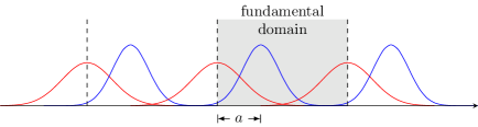
Figure 4.1: Overlap of two Gaussians on a torus. The overlap of a given, say red, curve is not just the overlap with one blue curve but with infinitely many of them, thus leading to an expression of the form (4.67).

Turning this around, the upper characteristics $\widehat{\alpha}$ in equations 3.30 and 4.67, or, more precisely, $\min\bigl{(}|\widehat{\alpha}/\lambda|,|1-\widehat{\alpha}/\lambda|\bigr{)}$ with $0\leq|\widehat{\alpha}/\lambda|<1$, has the interpretation of a “distance between the loci of the states”, i.e. $a$ in figure 4.1. We illustrate this by plotting some sample Yukawa couplings in figure 4.2. This geometric intuition may conceivably provide us with an understanding of the observed hierarchies of fermion masses. Apart from the fact that the kinetic terms are under control, the geometric interpretation may be one of the strongest motivations for deriving the modular flavor symmetries from explicit tori.

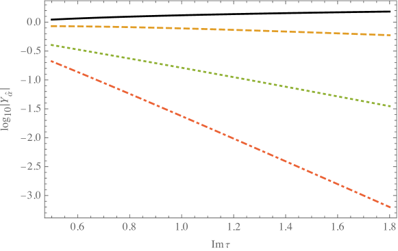
Figure 4.2: Dependence of the magnitude of the Yukawa couplings $Y_{\widehat{\alpha}}$ for $\operatorname{Re}\tau=0.1$. The black solid, orange dashed, green dotted and red dash–dotted curves represent $\widehat{\alpha}=0$, $1$, $2$ and $3$, respectively. There is an exponential suppression with $\operatorname{Im}\tau$ that depends on the “distance” between the wave functions $\widehat{\alpha}$, i.e. the $\operatorname{Im}\tau$ dependence is more pronounced for larger $\widehat{\alpha}$.

4.5.3 Model with $\mathcal{I}_{ab}=\mathcal{I}_{ca}=2$ and $\mathcal{I}_{bc}=-4$

Although we have stressed that our results are valid for odd repetitions of matter $\mathcal{I}_{\alpha\beta}$, they of course also apply to settings in which all $\mathcal{I}_{\alpha\beta}$ are even. Let us consider a toy model with the same superpotential and gauge group breaking as in section 4.5.2 by the fluxes

$$F =\frac{\pi\hskip 0.43057pt\mathrm{i}\hskip 0.43057pt}{\operatorname{Im}\tau}\begin{pmatrix}\mathds{1}_{2\times 2}&0&0\\ 0&\mathllap{-}2&0\\ 0&0&2\\ \end{pmatrix}\;,$$ (4.69)

where we used equation 3.1. This means that we have two repetitions of $L^{i}$ and $H^{j}$ each, and four copies of $R^{k}$. Similarly to what we have found in section 4.5.2, there are $\lambda/2+1=3$ independent Yukawa couplings,

$$Y_{0} :=Y_{i=j,j,k=2j}\;, Y_{1} :=Y_{i=j+1,j,k=2j+1}=Y_{3}:=Y_{i=j+1,j,k=2j+3}\;,$$ (4.70a)

$$Y_{2} :=Y_{i=j,j,k=2j+2}\;,$$ (4.70b)

where $i$ and $j$ are understood to be modulo $2$, and $k$ modulo $4$. The equality $Y_{1}=Y_{3}$ is also a consequence of the exchange symmetry given in equation 4.66. The four–plet of holomorphic Yukawa couplings $\mathcal{Y}_{\widehat{\alpha}}$ follow the modular transformations (4.43), with the matrices

$$\rho_{\boldsymbol{4}}(\widetilde{S})=-\,\frac{\mathrm{e}^{\hskip 0.3014pt\mathrm{i}\hskip 0.3014pt\frac{\pi}{4}}}{\sqrt{4}}\begin{pmatrix}1&1&1&1\\ 1&\hskip 0.43057pt\mathrm{i}\hskip 0.43057pt&-1&-\hskip 0.43057pt\mathrm{i}\hskip 0.43057pt\\ 1&-1&1&-1\\ 1&-\hskip 0.43057pt\mathrm{i}\hskip 0.43057pt&-1&\hskip 0.43057pt\mathrm{i}\hskip 0.43057pt\\ \end{pmatrix}\quad\text{and}\quad\rho_{\boldsymbol{4}}(\widetilde{T})=\begin{pmatrix}1&0&0&0\\ 0&\mathrm{e}^{\frac{\pi\hskip 0.21529pt\mathrm{i}\hskip 0.21529pt}{4}}&0&0\\ 0&0&-1&0\\ 0&0&0&\mathrm{e}^{\frac{\pi\hskip 0.21529pt\mathrm{i}\hskip 0.21529pt}{4}}\\ \end{pmatrix}\;.$$ (4.71)

Analogously to what we have done in section 4.5.2, due to the relations of the Yukawa couplings in equation 4.70, we can reduce the representation matrices through the projection matrix

$$P_{4\to 3} =\begin{pmatrix}1&0&0\\ 0&\frac{1}{\sqrt{2}}&0\\ 0&0&1\\ 0&\frac{1}{\sqrt{2}}&0\\ \end{pmatrix}\;.$$ (4.72a)

We can define the triplet of independent Yukawa couplings through $Y_{\boldsymbol{3}}=P_{4\to 3}^{T}Y_{\boldsymbol{4}}$, which transforms under the representation matrices given by

$$\rho_{\boldsymbol{3}}(\widetilde{S}) =P_{4\to 3}^{T}\rho_{\boldsymbol{4}}(\widetilde{S})P_{4\to 3}=-\,\frac{\mathrm{e}^{\hskip 0.3014pt\mathrm{i}\hskip 0.3014pt\frac{\pi}{4}}}{\sqrt{4}}\begin{pmatrix}1&\sqrt{2}&1\\ \sqrt{2}&0&-\sqrt{2}\\ 1&-\sqrt{2}&1\\ \end{pmatrix}\;,$$ (4.73a)

$$\rho_{\boldsymbol{3}}(\widetilde{T}) =P_{6\to 4}^{T}\rho_{\boldsymbol{6}}(\widetilde{T})P_{6\to 4}=\begin{pmatrix}1&0&0\\ 0&\mathrm{e}^{\frac{\pi\hskip 0.21529pt\mathrm{i}\hskip 0.21529pt}{4}}&0\\ 0&0&-1\\ \end{pmatrix}\;.$$ (4.73b)

The transformation matrices of the doublets $L^{i}$ and $H^{j}$ are obtained by setting $M=2$ in equation 4.48 and taking its conjugate. The resulting matrices are given by equation 4.55. The four–plets $R^{k}$ transform through equation 4.48 for $M=4$, that is

$$\rho_{\boldsymbol{4}^{\prime}}^{\phi}(\widetilde{S})=\frac{\mathrm{e}^{\hskip 0.3014pt\mathrm{i}\hskip 0.3014pt\frac{\pi}{4}}}{\sqrt{4}}\,\begin{pmatrix}1&1&1&1\\ 1&\hskip 0.43057pt\mathrm{i}\hskip 0.43057pt&-1&-\hskip 0.43057pt\mathrm{i}\hskip 0.43057pt\\ 1&-1&1&-1\\ 1&-\hskip 0.43057pt\mathrm{i}\hskip 0.43057pt&-1&\hskip 0.43057pt\mathrm{i}\hskip 0.43057pt\\ \end{pmatrix}\quad\text{and}\quad\rho_{\boldsymbol{4}^{\prime}}^{\phi}(\widetilde{T})=\begin{pmatrix}1&0&0&0\\ 0&\mathrm{e}^{-\frac{3\pi\hskip 0.21529pt\mathrm{i}\hskip 0.21529pt}{4}}&0&0\\ 0&0&-1&0\\ 0&0&0&\mathrm{e}^{-\frac{3\pi\hskip 0.21529pt\mathrm{i}\hskip 0.21529pt}{4}}\\ \end{pmatrix}\;.$$ (4.74)

The representation matrices in equations 4.55, 4.71, 4.73 and 4.74 fulfill the conditions (4.13) for $N=2$ and (4.14) which implies that we have a theory endowed with a $\widetilde{\Gamma}_{2\lambda=8}\cong[768,1085324]$ metaplectic flavor symmetry. In this model, the four–plet of the Yukawa couplings decomposes as $\boldsymbol{4}=\boldsymbol{3}\oplus\boldsymbol{1}^{\prime}$, where the singlet vanishes. On the other hand, the matter four–plets decompose as $\boldsymbol{4}^{\prime}=\boldsymbol{3}^{\prime}\oplus\boldsymbol{1}^{\prime\prime}$ whereas the matter doublets $\boldsymbol{2}$ are irreducible. While all these representations are unfaithful, the combination $\boldsymbol{4}^{\prime}\oplus\boldsymbol{2}$ provides us with a faithful representation content of $\widetilde{\Gamma}_{8}$. The tensor products of $\boldsymbol{4}^{\prime}$ and $\boldsymbol{2}$ produce all $\widetilde{\Gamma}_{8}$ representations.

4.5.4 Model with $\mathcal{I}_{ab}=1$, $\mathcal{I}_{ca}=2$ and $\mathcal{I}_{bc}=-3$

It is important to show that our conjecture (4.50) that we have a $\widetilde{\Gamma}_{2\lambda}$ invariant superpotential is not only valid for repeated values of $\mathcal{I}_{\alpha\beta}$. To this end we consider a toy model with the Yukawa couplings as in equation 4.58 and with gauge group breaking $\mathrm{U}(3)\rightarrow\mathrm{U}(1)_{a}\times\mathrm{U}(1)_{b}\times\mathrm{U}(1)_{c}$ by the fluxes

$$F =\frac{\pi\hskip 0.43057pt\mathrm{i}\hskip 0.43057pt}{\operatorname{Im}\tau}\begin{pmatrix}-1&0&0\\ 0&-2&0\\ 0&0&1\\ \end{pmatrix}\;.$$ (4.75)

Out of $3\cdot 2\cdot 1$ a priori possible Yukawa couplings, $\lambda/2+1=4$ are distinct

$$Y_{0} :=Y_{000}\;, Y_{1} :=Y_{011}=Y_{5}:=Y_{012}\;,$$ (4.76a)

$$Y_{3} :=Y_{010}\;, Y_{2} :=Y_{001}=Y_{4}:=Y_{002}\;,$$ (4.76b)

where $i$ can only be $0$, and $j$ and $k$ are understood to be modulo $2$ and $3$ respectively. As $d=1$, this setting has a comparatively large number of distinct couplings, i.e. $4$ out of $6$ entries are distinct whereas e.g. in the model of section 4.5.2 only $4$ out of $54$ a priori contractions have nontrivial distinct coefficients. In this case, $\mathcal{I}_{ab}\neq\mathcal{I}_{ca}$, so there is no exchange symmetry of the type (4.66), yet the number of independent Yukawa couplings gets reduced due to the symmetry $Y_{0jk}=Y_{0j,3-k}$. Unlike the transformation that ensured the equality of Yukawa entries in the model discussed in section 4.5.2, this symmetry is not a nontrivial outer automorphism of the 4D continuous gauge symmetries. The six–plet of holomorphic Yukawa couplings $\mathcal{Y}_{\widehat{\alpha}}$ transform with the matrices from equation 4.63 that can be reduced by using equation 4.64 to a four–plet, which then transforms according to equation 4.65. Furthermore, using equation 4.48, we see that the singlet $\phi^{0,\mathcal{I}_{ab}=1}$ is invariant under modular transformations, the doublet $\phi^{j,\mathcal{I}_{ca}=2}$ transforms with the representation matrices from equation 4.55, and the triplet $\phi^{k,\mathcal{I}_{cb}=3}$ transforms using equation 4.60. It can be shown that all these matrices satisfy the conditions (4.13) for $N=3$ and equation 4.15. Therefore, the superpotential is invariant under the finite metaplectic flavor symmetry $\widetilde{\Gamma}_{2\lambda=12}$ of order 2304.

4.6 Comments on the relation to bottom–up constructions

As we have seen, the models derived from explicit tori give rise to the finite metaplectic groups, which have been discussed e.g. in [15] in the context of bottom–up model building. The models presented here do not attempt to make an immediate connection to particle phenomenology. At first sight, it seems to be hard to derive the models of [15] from tori for at least two reasons:

1. our fields all have modular weight $-\nicefrac{{1}}{{2}}$ while in [15] they come with a variety of weights, and

2. we have additional symmetries like the outer automorphism symmetry (4.66) and residual gauge factors.

On the other hand, deriving the modular transformations from an explicit higher–dimensional model has the virtue that normalization of the fields is known at tree level, and that otherwise free parameters get fixed. Of course, the Kähler potential is not exact, apart from the usual 4D corrections there are additional terms contributing (cf. [49]), yet the point that there is a zeroth order classical form plus corrections, which are under control. On the other hand, in the SB approach every invariant Kähler potential is as good as others [31], and there are thus large uncertainties. An additional benefit of deriving the modular flavor symmetries from explicit tori is the geometrical intuition one can develop for the Yukawa couplings, cf. our discussion at the end of section 4.5.2.

One may now wonder if the price that one has to pay for all these benefits is the inability to construct semi–realistic models. In what follows, we will argue that this is not the case. First of all, the $\mathds{T}^{2}$ model is just a building block of a more complete story. As explained in [32], these models are dual to some intersecting $D$–brane constructions. Moreover, the couplings of the latter are closely related to heterotic string compactifications [50], which provide us with a large number of potentially realistic models [51]. These more complete settings come with a variety of modular weights [52]. Second, even if one is not adding more dimensions to the construction, fields with higher modular weights can emerge as composites of fields with modular weight $-\nicefrac{{1}}{{2}}$. That is, if “quarks” of a model with an $\mathrm{SU}(N_{c})$ have modular weights $-\nicefrac{{1}}{{2}}$, then the “baryons” will have weights $-\nicefrac{{N_{c}}}{{2}}$.

5 Comments on the role of supersymmetry

Let us comment on the role supersymmetry (SUSY) plays in the discussion. While Cremades et al. work in a supersymmetric theory, they mention [32, see the beginning of section 5.3] that their derivation “in principle is valid for toroidal compactifications where supersymmetry might be broken explicitly”. Of course, if one wants to claim that the couplings that one has computed are Yukawa couplings, one needs to make sure that one computes the overlap between two fermionic and one bosonic zero–modes. In supersymmetric models there is no problem because the superpartners are described by the same wave functions.

In a model without low–energy SUSY one may be worried that quantum corrections lead to uncontrollable corrections to the wave function of the scalar. This is generally a very valid concern, yet is as recently been observed that in the magnetized tori there is an interesting cancellation of corrections to the scalar mass [33, 34, 35, 36]. While this has not yet led to a complete solution of the hierarchy problem in the SM, it does suggest that in the context of the very models that we were led to consider for the sake of deriving modular flavor symmetries the situation is “better” than in other nonsupersymmetric completions of the SM with a high UV scale. In fact, similar cancellations have been reported in [53], where they were attributed to modular symmetries.

In a bit more detail, one could imagine a torus compactification in which the Yukawa couplings emerge as outlined in [32], namely as the overlap of three wave functions. These wave functions describe two fermions and one scalar, such as the SM Higgs. If the scalars remain light, they will still be approximate zero–modes, and thus the profile is approximately given by equation 2.1. So the Yukawa couplings will, to some good approximation, be the ones of equation 3.2. So supersymmetry is not instrumental for having models with modular flavor symmetries.

6 Summary

We discussed how modular flavor symmetries derive from explicit tori which are endowed with magnetic fluxes. Using Euler’s Theorem, we have derived a closed–form expression for the Yukawa couplings between zero modes. This expression generalizes the results of the literature to arbitrary flux parameters $\mathcal{I}_{ab}$ and $\mathcal{I}_{ca}$, which fix $\mathcal{I}_{bc}$, and is not restricted to the special case in which one flux parameter equals $1$. Each entry of the Yukawa tensor is a single $\vartheta$–function, i.e. the holomorphic Yukawa couplings take the form

$$\mathcal{Y}_{ijk}(\tau)=\vartheta\begin{bmatrix}\widehat{\alpha}_{ijk}/\lambda\\ 0\end{bmatrix}(0,\lambda\,\tau)\;,$$ (6.1)

where

$$\widehat{\alpha}_{ijk}=\mathcal{I}_{ca}^{\prime}\,i-\mathcal{I}_{ab}^{\prime}\,j+\mathcal{I}_{ca}^{\prime}\,\left(\mathcal{I}_{ab}^{\prime}\right)^{\phi(|\mathcal{I}_{bc}^{\prime}|)}\,(k-i-j)\mod\lambda\;.$$ (6.2)

Here, $\phi$ denotes the Euler $\phi$–function, $\mathcal{I}_{\alpha\beta}^{\prime}=\mathcal{I}_{\alpha\beta}/d$ for $\alpha,\beta\in\{a,b,c\}$, $d=\gcd\bigl{(}|\mathcal{I}_{ab}|,|\mathcal{I}_{ca}|,|\mathcal{I}_{bc}|\bigr{)}$, $\lambda=\operatorname{lcm}\bigl{(}|\mathcal{I}_{ab}|,|\mathcal{I}_{ca}|,|\mathcal{I}_{bc}|\bigr{)}$, and $\tau$ denotes the half–period ratio of the torus. The condensed form for holomorphic Yukawa couplings as single $\vartheta$–functions is instrumental for deriving the symmetries between Yukawa couplings. As we have seen, these symmetries include outer automorphisms of the low–energy gauge symmetry. These couplings are modular forms of weight $\nicefrac{{1}}{{2}}$ of level $2\lambda$ that build representations under the metaplectic modular flavor symmetry $\widetilde{\Gamma}_{2\lambda}$. There are at most $1+\lambda/2$ distinct Yukawa couplings, which transform as a (generically reducible) representation $\boldsymbol{\lambda}$ of $\widetilde{\Gamma}_{2\lambda}$. This means that e.g. a model with flux parameters $(\mathcal{I}_{ab},\mathcal{I}_{ca},\mathcal{I}_{bc})=(1,2,-3)$ has as many independent Yukawa couplings as a model with fluxes $(3,3,-6)$. We have commented on the geometric interpretation of the Yukawa couplings, and that the $\widehat{\alpha}_{ijk}$ in equation 6.1 corresponds to a separation of the states, and lead to an exponential suppression with an exponent $\min(\widehat{\alpha}_{ijk},1-\widehat{\alpha}_{ijk})\,\operatorname{Im}\tau$ for unsuppressed $\operatorname{Im}\tau$. The 4D fields have a well–defined transformation behavior under $\widetilde{\Gamma}_{2\lambda}$, regardless of whether the flux is even or odd, and have weight $k_{\phi}=-\nicefrac{{1}}{{2}}$. Our analysis is restricted to a magnetized torus $\mathds{T}^{2}$ and its half–period ratio $\tau$, which is contained in the so–called complex structure modulus. We also set the Wilson lines to zero, and largely disregarded the Kähler modulus. While this is sufficient to derive meaningful modular flavor symmetries, this analysis may be thought of as a building block of more complete, perhaps stringy models. It will be interesting to derive a generalization of equation 6.1 for such constructions.

We have also commented on the role that supersymmetry plays in these constructions. As already pointed out in [32], supersymmetry is not instrumental as long as the profiles of the zero–modes do not get distorted too much. More recent analyses [33, 34, 35, 36] indicate that magnetized tori have certain unusual properties in that scalar masses seem to be immune to quantum corrections even without supersymmetry. This means that one can plausibly disentangle modular flavor symmetries from the question of low–energy supersymmetry.

Acknowledgments

The work of Y.A. was supported by Kuwait University. The work of M.-C.C., M.R. and S.S. was supported by the National Science Foundation, under Grant No. PHY-1915005. The work of S.R.-S. was partly supported by CONACyT grant F-252167. This work is also supported by UC-MEXUS-CONACyT grant No. CN-20-38.

Appendix A $\vartheta$–functions

In this appendix, we collect some relevant facts on the $\vartheta$–functions. Our conventions are based on [37] and [54]. One defines

$$\vartheta\begin{bmatrix}\!\alpha\!\\[1.29167pt] \!\beta\!\end{bmatrix}(z,\tau):=S_{\beta}\,T_{\alpha}\,\vartheta(z,\tau)=\mathrm{e}^{2\pi\hskip 0.3014pt\mathrm{i}\hskip 0.3014pt\,\alpha\,\beta}\,T_{\alpha}\,S_{\beta}\,\vartheta(z,\tau)\;,$$ (A.1)

where [37, p. 4]

$$\vartheta(z,\tau):=\sum\limits_{\ell\in\mathds{Z}}\exp(\hskip 0.43057pt\mathrm{i}\hskip 0.43057pt\,\pi\,\ell^{2}\,\tau)\,\exp(2\pi\hskip 0.43057pt\mathrm{i}\hskip 0.43057pt\,\ell\,z)$$ (A.2)

with $\operatorname{Im}\tau>0$, and [37, p. 6]

$$(S_{\beta}f)(z) := f(z+\beta)\;,$$ (A.3a)

$$(T_{\alpha}f)(z) := \mathrm{e}^{\hskip 0.3014pt\mathrm{i}\hskip 0.3014pt\,\pi\,\alpha^{2}\,\tau+2\pi\hskip 0.3014pt\mathrm{i}\hskip 0.3014pt\,\alpha\,z}\,f(z+\alpha\,\tau)\;.$$ (A.3b)

This immediately gives us (cf. [54, p. 214 f.])

$$\vartheta\begin{bmatrix}\!\alpha\!\\[1.29167pt] \!\beta\!\end{bmatrix}(z,\tau)=\sum\limits_{\ell=-\infty}^{\infty}\mathrm{e}^{\hskip 0.3014pt\mathrm{i}\hskip 0.3014pt\pi\,(\alpha+\ell)^{2}\,\tau}\,\mathrm{e}^{2\pi\hskip 0.3014pt\mathrm{i}\hskip 0.3014pt\,(\alpha+\ell)\,(z+\beta)}\;.$$ (A.4)

For an integer $n\in\mathds{Z}$ one has torus periodicities

$$\vartheta\begin{bmatrix}\!\alpha\!\\[1.29167pt] \!\beta\!\end{bmatrix}(z+n,\tau) =\mathrm{e}^{2\pi\hskip 0.3014pt\mathrm{i}\hskip 0.3014pt\,n\,\alpha}\,\vartheta\begin{bmatrix}\!\alpha\!\\[1.29167pt] \!\beta\!\end{bmatrix}(z,\tau)\;,$$ (A.5a)

$$\vartheta\begin{bmatrix}\!\alpha\!\\[1.29167pt] \!\beta\!\end{bmatrix}(z+n\,\tau,\tau) =\mathrm{e}^{-\hskip 0.3014pt\mathrm{i}\hskip 0.3014pt\pi\,n^{2}\,\tau-2\pi\hskip 0.3014pt\mathrm{i}\hskip 0.3014pt\,n\,(z+\beta)}\,\vartheta\begin{bmatrix}\!\alpha\!\\[1.29167pt] \!\beta\!\end{bmatrix}(z,\tau)\;.$$ (A.5b)

Further, the $\vartheta$–function have several periodicities in the characteristics $\alpha$ and $\beta$,

$$\vartheta\begin{bmatrix}\!\alpha+1\!\\[1.29167pt] \!\beta\!\end{bmatrix}(z,\tau) =\vartheta\begin{bmatrix}\!\alpha\!\\[1.29167pt] \!\beta\!\end{bmatrix}(z,\tau)\;,$$ (A.6a)

$$\vartheta\begin{bmatrix}\!\alpha\!\\[1.29167pt] \!\beta+1\!\end{bmatrix}(z,\tau) =\mathrm{e}^{2\pi\hskip 0.3014pt\mathrm{i}\hskip 0.3014pt\,\alpha}\,\vartheta\begin{bmatrix}\!\alpha\!\\[1.29167pt] \!\beta\!\end{bmatrix}(z,\tau)\;.$$ (A.6b)

The behavior under modular transformation is

$$\vartheta\begin{bmatrix}\!\alpha\!\\[1.29167pt] \!\beta\!\end{bmatrix}(z,\tau+1) =\mathrm{e}^{-\hskip 0.3014pt\mathrm{i}\hskip 0.3014pt\,\pi\,\alpha\,(\alpha+1)}\,\vartheta\begin{bmatrix}\!\alpha\!\\[1.29167pt] \!\beta+\alpha+\frac{1}{2}\!\end{bmatrix}(z,\tau)\;,$$ (A.7a)

$$\vartheta\begin{bmatrix}\!\alpha\!\\[1.29167pt] \!\beta\!\end{bmatrix}\left(-\frac{z}{\tau},-\frac{1}{\tau}\right) =\sqrt{-\hskip 0.43057pt\mathrm{i}\hskip 0.43057pt\,\tau}\,\mathrm{e}^{2\pi\hskip 0.3014pt\mathrm{i}\hskip 0.3014pt\,\left(\frac{z^{2}}{2\tau}+\alpha\,\beta\right)}\,\vartheta\begin{bmatrix}\!-\beta\!\\[1.29167pt] \!\alpha\!\end{bmatrix}(z,\tau)\;.$$ (A.7b)

Another useful formula is

$$\vartheta\begin{bmatrix}\!0\!\\[1.29167pt] \!\nicefrac{{j}}{{M}}\!\end{bmatrix}\left(z,\frac{\tau}{M}\right) =\sum_{k=0}^{M-1}e^{2\pi\text{i}jk/M}\vartheta\begin{bmatrix}\frac{k}{M}\\ 0\end{bmatrix}(Mz,M\tau)\;.$$ (A.8)

Appendix B Torus integration

The torus is defined by two lattice vectors, which can be chosen as $e_{1}=2\pi R$ and $e_{2}=2\pi R\,\tau$, where the real, dimensionful quantity $R$ sets the length of one lattice vector, and $\tau$ with $\operatorname{Im}\tau>0$ is the half–period ratio. In this basis, the torus metric reads

$$G=(2\pi R)^{2}\begin{pmatrix}1&\operatorname{Re}\tau\\ \operatorname{Re}\tau&|\tau|^{2}\end{pmatrix}\;.$$ (B.1)

We can define the fundamental domain of the torus as

$$\mathds{T}^{2}=\{{z}\in\mathds{C}\;;~{}~{}z=x\,e_{1}+y\,e_{2}\ \text{ with }\ 0\leq x,y\leq 1\}\;.$$ (B.2)

It is straightforward to verify that the Jacobian of the transformation $(\operatorname{Re}z,\operatorname{Im}z)\mapsto(x,y)$ is given by $(2\pi R)^{2}\operatorname{Im}\tau$. Therefore, the integrals of an arbitrary function $f(z)$ over the fundamental domain are given by

$$\int\limits_{\mathbb{T}^{2}}\!\mathop{}\!\mathrm{d}^{2}z\,f(z)=(2\pi R)^{2}\operatorname{Im}\tau\,\int\limits_{0}^{1}\!\mathop{}\!\mathrm{d}x\,\int\limits_{0}^{1}\!\mathop{}\!\mathrm{d}y\,f(xe_{1}+ye_{2})\;.$$ (B.3)

Let us now look at constant modes on the torus, or, equivalently integrate over the torus $\mathds{T}^{2}$ to determine its volume. We then have

$$\operatorname{vol}(\text{torus})=\int\limits_{\mathds{T}^{2}}\!\mathop{}\!\mathrm{d}^{2}z\,1=(2\pi R)^{2}\operatorname{Im}\tau=:\mathcal{A}\;.$$ (B.4)

Appendix C Explicit verification of the boundary conditions for transformed wave functions

C.1 $S$ transformation

We now compute the $S$ transformation, $\tau\mapsto-1/\tau$ (cf. equation 4.3), of equation 2.1. We have

$$\psi^{j,M}\left(-\frac{z}{\tau},-\frac{1}{\tau},0\right)=\bigg{(}\frac{2M\operatorname{Im}\frac{-1}{\tau}}{{\mathcal{A}}^{2}}\bigg{)}^{1/4}\exp\bigg{(}\hskip 0.43057pt\mathrm{i}\hskip 0.43057pt\pi M\frac{z}{\tau}\frac{\operatorname{Im}\frac{z}{\tau}}{\operatorname{Im}\frac{-1}{\tau}}\bigg{)}\,\vartheta\begin{bmatrix}\!\frac{j}{M}\!\\[1.29167pt] \!0\!\end{bmatrix}\bigg{(}-\frac{Mz}{\tau},-\frac{M}{\tau}\bigg{)}$$

$$=\frac{\mathcal{N}}{\sqrt{|\tau|}}\exp\bigg{(}\hskip 0.43057pt\mathrm{i}\hskip 0.43057pt\pi M\frac{z}{\tau}\frac{\operatorname{Im}{z\bar{\tau}}}{\operatorname{Im}{\tau}}\bigg{)}\sqrt{-\hskip 0.43057pt\mathrm{i}\hskip 0.43057pt\frac{\tau}{M}}\mathrm{e}^{2\pi M\hskip 0.3014pt\mathrm{i}\hskip 0.3014pt\frac{z^{2}}{2\tau}}\,\vartheta\begin{bmatrix}\!0\!\\[1.29167pt] \!\frac{j}{M}\!\end{bmatrix}\bigg{(}z,\frac{\tau}{M}\bigg{)}$$

$$=\frac{\mathcal{N}}{\sqrt{|\tau|}}\exp\bigg{(}\hskip 0.43057pt\mathrm{i}\hskip 0.43057pt\pi M\frac{z}{\tau}\frac{\operatorname{Im}{z\bar{\tau}}}{\operatorname{Im}{\tau}}\bigg{)}\sqrt{-\hskip 0.43057pt\mathrm{i}\hskip 0.43057pt\frac{\tau}{M}}\mathrm{e}^{\hskip 0.3014pt\mathrm{i}\hskip 0.3014pt\pi M\frac{z^{2}}{\tau}}\sum_{k=0}^{M-1}\mathrm{e}^{2\pi\hskip 0.3014pt\mathrm{i}\hskip 0.3014pt\,jk/M}\,\vartheta\begin{bmatrix}\!\frac{k}{M}\!\\[1.29167pt] \!0\!\end{bmatrix}(Mz,M\tau)$$

$$=\frac{\mathrm{e}^{{\frac{\hskip 0.21529pt\mathrm{i}\hskip 0.21529pt\pi}{4}}}}{\sqrt{M}}\bigg{(}{-}\frac{\tau}{|\tau|}\bigg{)}^{1/2}\sum_{k=0}^{M-1}\mathrm{e}^{\frac{2\pi\hskip 0.21529pt\mathrm{i}\hskip 0.21529ptjk}{M}}\bigg{[}\mathcal{N}\exp\bigg{(}\frac{\hskip 0.43057pt\mathrm{i}\hskip 0.43057pt\pi Mz}{\tau}{\frac{\operatorname{Im}z\bar{\tau}}{\operatorname{Im}\tau}}+\hskip 0.43057pt\mathrm{i}\hskip 0.43057ptM\pi\frac{z^{2}}{\tau}\bigg{)}\,\vartheta\begin{bmatrix}\!\frac{k}{M}\!\\[1.29167pt] \!0\!\end{bmatrix}(Mz,M\tau)\bigg{]}$$

$$=\frac{\mathrm{e}^{{\hskip 0.3014pt\mathrm{i}\hskip 0.3014pt}\frac{\pi}{4}}}{\sqrt{M}}\bigg{(}{-}\frac{\tau}{|\tau|}\bigg{)}^{1/2}\sum_{k=0}^{M-1}\mathrm{e}^{\frac{2\pi\hskip 0.21529pt\mathrm{i}\hskip 0.21529ptjk}{M}}\mathcal{N}\mathrm{e}^{i\pi Mz\frac{\operatorname{Im}z}{\operatorname{Im}\tau}}\,\vartheta\begin{bmatrix}\!\frac{j}{M}\!\\[1.29167pt] \!0\!\end{bmatrix}(Mz,M\tau)\;,$$ (C.1)

where we used (2.2), (A.7b) and (A.8) in the first, second and third lines respectively. We thus arrive at (C.2). Therefore, the $S$ modular transformation of the zero modes is

$$\psi^{j,M}\left(-\frac{z}{\tau},-\frac{1}{\tau},0\right) =\frac{\mathrm{e}^{{\hskip 0.3014pt\mathrm{i}\hskip 0.3014pt}\frac{\pi}{4}}}{\sqrt{M}}\bigg{(}{-}\frac{\tau}{|\tau|}\bigg{)}^{1/2}\sum_{k=0}^{M-1}\mathrm{e}^{2\pi\hskip 0.3014pt\mathrm{i}\hskip 0.3014ptjk/M}\,\psi^{k,M}(z,\tau,0)\;.$$ (C.2)

It is straightforward to see that the wave function of equation C.2 satisfies the boundary conditions of equations 4.27a and 4.27b. Note that

$$\psi^{j,M}\bigg{(}-\frac{z}{\tau}+1,-\frac{1}{\tau},0\bigg{)}=\psi^{j,M}\bigg{(}-\frac{(z-\tau)}{\tau},-\frac{1}{\tau},0\bigg{)}\\ =\frac{\mathrm{e}^{{\hskip 0.3014pt\mathrm{i}\hskip 0.3014pt}\frac{\pi}{4}}}{\sqrt{M}}\bigg{(}{-}\frac{\tau}{|\tau|}\bigg{)}^{1/2}\sum_{k=0}^{M-1}\mathrm{e}^{\frac{2\pi\hskip 0.21529pt\mathrm{i}\hskip 0.21529ptjk}{M}}\,\psi^{k,M}(z-\tau,\tau,0)=\exp\bigg{(}-\hskip 0.43057pt\mathrm{i}\hskip 0.43057pt\pi M\frac{\operatorname{Im}z\bar{\tau}}{\operatorname{Im}\tau}\bigg{)}\,\psi^{j,M}\bigg{(}-\frac{z}{\tau},-\frac{1}{\tau},0\bigg{)}$$ (C.3)

and

$$\psi^{j,M}\bigg{(}-\frac{z}{\tau}-\frac{1}{\tau},-\frac{1}{\tau},0\bigg{)}=\psi^{j,M}\bigg{(}-\frac{(z+1)}{\tau},-\frac{1}{\tau},0\bigg{)}\\ =\frac{\mathrm{e}^{{\hskip 0.3014pt\mathrm{i}\hskip 0.3014pt}\frac{\pi}{4}}}{\sqrt{M}}\bigg{(}{-}\frac{\tau}{|\tau|}\bigg{)}^{1/2}\sum_{k=0}^{M-1}\mathrm{e}^{\frac{2\pi\hskip 0.21529pt\mathrm{i}\hskip 0.21529ptjk}{M}}\psi^{k,M}(z+1,\tau,0)=\exp\bigg{(}\frac{\hskip 0.43057pt\mathrm{i}\hskip 0.43057pt\pi M\operatorname{Im}z}{\operatorname{Im}\tau}\bigg{)}\psi^{j,M}\bigg{(}-\frac{z}{\tau},-\frac{1}{\tau},0\bigg{)}\;.$$ (C.4)

Thus, from equations C.3 and C.4 we can see that the $S$ transformed zero mode follows the boundary conditions of equations 4.27a and 4.27b for both odd and even $M$.

C.2 $T$ transformation

Now, we compute the transformed wave function $\psi^{j,M}(z,\tau+1,0)$ and check that it satisfies both equation 4.28a and equation 4.28b. Applying the $T$ modular transformation in equation 2.1 gives

$$\psi^{j,M}(z,\tau+1,0) =\mathcal{N}\mathrm{e}^{\hskip 0.3014pt\mathrm{i}\hskip 0.3014pt\pi\,Mz\frac{\operatorname{Im}z}{\operatorname{Im}\tau}}\vartheta\begin{bmatrix}\!\frac{j}{M}\!\\[1.29167pt] \!0\!\end{bmatrix}\bigl{(}Mz,M(\tau+1),0\bigr{)}$$

$$=\mathrm{e}^{-\hskip 0.3014pt\mathrm{i}\hskip 0.3014pt\,\pi j\bigl{(}\frac{j}{M}+1\bigr{)}}\,\mathcal{N}\mathrm{e}^{\hskip 0.3014pt\mathrm{i}\hskip 0.3014pt\,\pi Mz\frac{\operatorname{Im}z}{\operatorname{Im}\tau}}\,\vartheta\begin{bmatrix}\!\frac{j}{M}\!\\[1.29167pt] \!j+\frac{M}{2}\!\end{bmatrix}(Mz,M\tau)$$

$$=\mathrm{e}^{-\hskip 0.3014pt\mathrm{i}\hskip 0.3014pt\,\pi j\bigl{(}\frac{j}{M}+1\bigr{)}}\,\mathcal{N}\mathrm{e}^{\hskip 0.3014pt\mathrm{i}\hskip 0.3014pt\,\pi Mz\frac{\operatorname{Im}z}{\operatorname{Im}\tau}}\,\mathrm{e}^{2\pi\hskip 0.3014pt\mathrm{i}\hskip 0.3014pt\,\frac{j}{M}j}\vartheta\begin{bmatrix}\!\frac{j}{M}\!\\[1.29167pt] \!\frac{M}{2}\!\end{bmatrix}(Mz,M\tau)$$

$$=\mathrm{e}^{-\hskip 0.3014pt\mathrm{i}\hskip 0.3014pt\,\pi j\bigl{(}1-\frac{j}{M}\bigr{)}}\,\mathcal{N}\mathrm{e}^{\hskip 0.3014pt\mathrm{i}\hskip 0.3014pt\,\pi Mz\frac{\operatorname{Im}z}{\operatorname{Im}\tau}}\,\vartheta\begin{bmatrix}\!\frac{j}{M}\!\\[1.29167pt] \!\frac{M}{2}\!\end{bmatrix}(Mz,M\tau)\;,$$ (C.5)

where we used (A.7a) and (A.6b) in the second and third line, respectively. Defining $\widetilde{\mathcal{N}}:=\mathrm{e}^{-\hskip 0.3014pt\mathrm{i}\hskip 0.3014pt\,\pi j\bigl{(}1-\frac{j}{M}\bigr{)}}\mathcal{N}$ we can thus write

$$\psi^{j,M}(z,\tau+1,0)=\widetilde{\mathcal{N}}\mathrm{e}^{\hskip 0.3014pt\mathrm{i}\hskip 0.3014pt\,\pi Mz\frac{\operatorname{Im}z}{\operatorname{Im}\tau}}\vartheta\begin{bmatrix}\!\frac{j}{M}\!\\[1.29167pt] \!\frac{M}{2}\!\end{bmatrix}(Mz,M\tau)\;.$$ (C.6)

Now we check that equation C.6 satisfies boundary conditions given by equations 4.28a and 4.28b. The first boundary condition is satisfied as shifting $z\rightarrow z+1$ in equation C.6 gives

$$\psi^{j,M}(z+1,\tau+1,0)~{} =~{}\widetilde{\mathcal{N}}\mathrm{e}^{\hskip 0.3014pt\mathrm{i}\hskip 0.3014pt\,\pi M(z+1)\frac{\operatorname{Im}z}{\operatorname{Im}\tau}}\vartheta\begin{bmatrix}\!\frac{j}{M}\!\\[1.29167pt] \!\frac{M}{2}\!\end{bmatrix}(M(z+1),M\tau)$$

$$=~{}\exp\bigg{(}\hskip 0.43057pt\mathrm{i}\hskip 0.43057pt\,\frac{\pi M\operatorname{Im}z}{\operatorname{Im}\tau}\bigg{)}\,\widetilde{\mathcal{N}}\mathrm{e}^{\hskip 0.3014pt\mathrm{i}\hskip 0.3014pt\,\pi M(z+1)\frac{\operatorname{Im}z}{\operatorname{Im}\tau}}\mathrm{e}^{2\pi\hskip 0.3014pt\mathrm{i}\hskip 0.3014pt\,M\frac{j}{M}}\vartheta\begin{bmatrix}\!\frac{j}{M}\!\\[1.29167pt] \!\frac{M}{2}\!\end{bmatrix}(Mz,M\tau)$$

$$=~{}\exp\bigg{(}\hskip 0.43057pt\mathrm{i}\hskip 0.43057pt\,\frac{\pi M\operatorname{Im}z}{\operatorname{Im}\tau}\bigg{)}\psi^{j,M}(z,\tau+1,0)\;,$$ (C.7)

where we used equation A.5a in the second line. For equation 4.28b we have

$$\psi^{j,M}(z+\tau+1,\tau+1,0)=\widetilde{\mathcal{N}}\mathrm{e}^{\frac{\hskip 0.21529pt\mathrm{i}\hskip 0.21529pt\,\pi M(z+\tau+1)}{\operatorname{Im}\tau}\operatorname{Im}(z+\tau+1)}\vartheta\begin{bmatrix}\!\frac{j}{M}\!\\[1.29167pt] \!\frac{M}{2}\!\end{bmatrix}(M(z+\tau+1),M\tau)$$

$$=\widetilde{\mathcal{N}}\mathrm{e}^{\frac{\hskip 0.21529pt\mathrm{i}\hskip 0.21529pt\,\pi M}{\operatorname{Im}\tau}[z\operatorname{Im}z+(\tau+1)\operatorname{Im}z+z\operatorname{Im}(\tau+1)+(\tau+1)\operatorname{Im}(\tau+1)}\,\mathrm{e}^{2\pi\hskip 0.3014pt\mathrm{i}\hskip 0.3014pt\,\frac{j}{M}M}\vartheta\begin{bmatrix}\!\frac{j}{M}\!\\[1.29167pt] \!\frac{M}{2}\!\end{bmatrix}(M(z+\tau),M\tau)$$

$$=\widetilde{\mathcal{N}}\mathrm{e}^{\frac{\hskip 0.21529pt\mathrm{i}\hskip 0.21529pt\,\pi M}{\operatorname{Im}\tau}[z\operatorname{Im}z+(\tau+1)\operatorname{Im}z+z\operatorname{Im}(\tau+1)+(\tau+1)\operatorname{Im}(\tau+1)}\,\mathrm{e}^{-\pi\hskip 0.3014pt\mathrm{i}\hskip 0.3014pt\,\tau M-2\pi\hskip 0.3014pt\mathrm{i}\hskip 0.3014pt\,(Mz+{\frac{M}{2})}}\vartheta\begin{bmatrix}\!\frac{j}{M}\!\\[1.29167pt] \!\frac{M}{2}\!\end{bmatrix}(Mz,M\tau)$$

$$=\mathrm{e}^{\frac{\hskip 0.21529pt\mathrm{i}\hskip 0.21529pt\,\pi M}{\operatorname{Im}\tau}[(\tau+1)\operatorname{Im}z+z\operatorname{Im}(\tau+1)+(\tau+1)\operatorname{Im}(\tau+1)-\tau\operatorname{Im}\tau-2z\operatorname{Im}\tau-\operatorname{Im}\tau]}\,\widetilde{\mathcal{N}}\mathrm{e}^{\frac{\hskip 0.21529pt\mathrm{i}\hskip 0.21529pt\,\pi M}{\operatorname{Im}\tau}z\operatorname{Im}z}\vartheta\begin{bmatrix}\!\frac{j}{M}\!\\[1.29167pt] \!\frac{M}{2}\!\end{bmatrix}(Mz,M\tau)$$

$$=\exp\bigg{(}\frac{\hskip 0.43057pt\mathrm{i}\hskip 0.43057pt\,\pi M}{\operatorname{Im}\tau}\operatorname{Im}(\bar{\tau}+1)z\bigg{)}\,\psi^{j,M}(z,\tau+1,0)\;,$$ (C.8)

where we have used equations A.5a and A.5b in the second and third line respectively. Therefore, the transformed modular wave function given by equation C.6 follows the transformed boundary conditions of equations 4.28a and 4.28b for even and odd $M$.

Let us now tackle the problem of expressing the $T$ transformed wave functions in terms of the original ones. As noted in section (4.4.1), for odd values of $M$ it is not possible to express the $T$ transformed wave functions in terms of the original ones because of (4.30). At the level of the wave functions, one can refer to equation C.6 and see that if $M$ is even, then using (A.6b) confirms (4.31). However, if $M$ is odd, in order to make use of (A.6b) we need to shift the $z$ coordinate as $z\mapsto z+\Delta z$ with real $\Delta z$. Using equation C.6 we have

$$\psi^{j,M}(z+\Delta z,\tau+1,0)=\widetilde{\mathcal{N}}\mathrm{e}^{\hskip 0.3014pt\mathrm{i}\hskip 0.3014pt\,\pi M(z+\Delta z)\frac{\operatorname{Im}z}{\operatorname{Im}\tau}}\vartheta\begin{bmatrix}\!\frac{j}{M}\!\\[1.29167pt] \!\frac{M}{2}\!\end{bmatrix}(M(z+\Delta z),M\tau)$$

$$=\widetilde{\mathcal{N}}\mathrm{e}^{\hskip 0.3014pt\mathrm{i}\hskip 0.3014pt\,\pi M\Delta z\frac{\operatorname{Im}z}{\operatorname{Im}\tau}}\mathrm{e}^{\hskip 0.3014pt\mathrm{i}\hskip 0.3014pt\,\pi Mz\frac{\operatorname{Im}z}{\operatorname{Im}\tau}}\vartheta\begin{bmatrix}\!\frac{j}{M}\!\\[1.29167pt] \!0\!\end{bmatrix}(M(z+\Delta z+\tfrac{1}{2}),M\tau),$$ (C.9)

where we have used (A.4) to rewrite the lower characteristic of the $\vartheta$–function as a shift in the $z$ coordinate. Therefore, if we assume that $\Delta z$ is a half–integer number, we can use (A.5a) which gives

$$\psi^{j,M}(z+\Delta z,\tau+1,0)=\widetilde{\mathcal{N}}\mathrm{e}^{\hskip 0.3014pt\mathrm{i}\hskip 0.3014pt\,\pi M\Delta z\frac{\operatorname{Im}z}{\operatorname{Im}\tau}}\mathrm{e}^{\hskip 0.3014pt\mathrm{i}\hskip 0.3014pt\,\pi Mz\frac{\operatorname{Im}z}{\operatorname{Im}\tau}}\mathrm{e}^{2\pi\hskip 0.3014pt\mathrm{i}\hskip 0.3014ptj(\frac{1}{2}+\Delta z)}\vartheta\begin{bmatrix}\!\frac{j}{M}\!\\[1.29167pt] \!0\!\end{bmatrix}(Mz,M\tau)$$

$$=\mathrm{e}^{\hskip 0.3014pt\mathrm{i}\hskip 0.3014pt\,\pi M\Delta z\frac{\operatorname{Im}z}{\operatorname{Im}\tau}}\mathrm{e}^{\pi\hskip 0.3014pt\mathrm{i}\hskip 0.3014ptj\left(\frac{j}{M}+2\Delta z\right)}\psi^{j,M}(z,\tau,0).$$ (C.10)

Note that in order to use (A.5a), $M\left(\frac{1}{2}+\Delta z\right)$ needs to be an integer. Therefore, for odd $M$, $\Delta z$ needs to be half–integer, whereas for even $M$ both integer and half–integer $\Delta z$ are valid choices. After a redefinition of $z\rightarrow z-\Delta z$ with some half–integer $\Delta z$,

$$\psi^{j,M}(z,\tau,0)\xmapsto{~{}T~{}}\mathrm{e}^{\hskip 0.3014pt\mathrm{i}\hskip 0.3014pt\pi M\Delta z\frac{\operatorname{Im}z}{\operatorname{Im}\tau}}\mathrm{e}^{\hskip 0.3014pt\mathrm{i}\hskip 0.3014pt\pi\frac{j^{2}}{|M|}+2\hskip 0.3014pt\mathrm{i}\hskip 0.3014pt\pi j\Delta z}\,\psi^{j,M}(z-\Delta z,\tau,0)\;,$$ (C.11)

and this is valid for both even and odd values of $M$.

Appendix D Symmetries between the Yukawa couplings

In this appendix we identify additional relations between the Yukawa couplings given in equation 3.30. Yukawa entries with different $i$, $j$ and/or $k$ are equal if the upper characteristic,

$$\frac{\mathcal{I}_{ca}^{\prime}\,i-\mathcal{I}_{ab}^{\prime}\,j+\mathcal{I}_{ca}^{\prime}\,\left(\mathcal{I}_{ab}^{\prime}\right)^{\phi\left(|\mathcal{I}_{bc}^{\prime}|\right)}\,(k-i-j)}{\lambda}=:u_{ijk}\;,$$ (D.1)

with $\mathcal{I}_{\alpha\beta}^{\prime}=\mathcal{I}_{\alpha\beta}/d$, is the same. For instance, suppose $i^{\prime}=i+r$, $j^{\prime}=j+s$ and $k^{\prime}=k+r+s$, so that $i^{\prime},\,j^{\prime}$ and $k^{\prime}$ also satisfy the selection rule (cf. equation 3.16). Then, for values of $r$ and $s$ satisfying

$$\mathcal{I}_{ca}\,r-\mathcal{I}_{ab}\,s=0\;,$$ (D.2)

we find that $u_{ijk}=u_{i^{\prime}\,j^{\prime}\,k^{\prime}}$, thus implying that $Y_{ijk}=Y_{i^{\prime}\,j^{\prime}\,k^{\prime}}$. We know that $\mathcal{I}_{ca}$ and $\mathcal{I}_{ab}$ are divisible by $d=\gcd\bigl{(}|\mathcal{I}_{ab}|,|\mathcal{I}_{ca}|,|\mathcal{I}_{bc}|\bigr{)}$ (cf. equation 3.12), $u_{ijk}$ has the form

$$u_{ijk}=\frac{\widehat{\alpha}_{ijk}}{\lambda}$$ (D.3)

with some integer $\widehat{\alpha}_{ijk}$ given by equation 6.2. Further, as a shift of $u_{ijk}$ by $1$ leaves the $\vartheta$–function in the Yukawa entry invariant (cf. equation A.6a), there are at most ${\lambda}$ distinct entries, i.e.

$$u_{ijk}\in\{0,1/{\lambda},\dots({\lambda}-1)/{\lambda}\}\;.$$ (D.4)

Additionally, for vanishing Wilson lines, the $\vartheta$–function takes the simple form (cf. equation A.4)

$$\vartheta\begin{bmatrix}\frac{\widehat{\alpha}_{ijk}}{{\lambda}}\\ 0\end{bmatrix}(0,{\lambda}\,\tau)=\sum\limits_{\ell=-\infty}^{\infty}\mathrm{e}^{\hskip 0.3014pt\mathrm{i}\hskip 0.3014pt\pi\,(\widehat{\alpha}_{ijk}/\lambda+\ell)^{2}\,{\lambda}\tau}\;,$$ (D.5)

which shows that

$$\vartheta\begin{bmatrix}-\frac{\widehat{\alpha}_{ijk}}{{\lambda}}\\ 0\end{bmatrix}(0,{\lambda}\,\tau)=\vartheta\begin{bmatrix}\frac{\widehat{\alpha}_{ijk}}{{\lambda}}\\ 0\end{bmatrix}(0,{\lambda}\,\tau)\;.$$ (D.6)

Therefore, there are ${\lambda}/2-1$ additional relations between the Yukawa couplings, and we have at most ${\lambda}/2+1$ distinct entries. These additional relations can manifest themselves in different ways. For instance, if $\mathcal{I}_{ab}=\mathcal{I}_{ca}$, the overlap integral (3.2) becomes

$$Y_{ijk}=g\,\sigma_{abc}\,\int\limits_{\mathds{T}^{2}}\!\mathop{}\!\mathrm{d}^{2}z\,\psi^{i,\mathcal{I}_{ab}}(z,\tau,\zeta)\,\psi^{j,\mathcal{I}_{ab}}(z,\tau,\zeta)\,\left(\psi^{k,\mathcal{I}_{cb}}(z,\tau,\zeta)\right)^{*}\;.$$ (D.7)

This equation is symmetric under $i\leftrightarrow j$, which implies that

$$Y_{ijk}=Y_{jik}\;.$$ (D.8)

As we discuss around equation 4.66 in the main text, the $i\leftrightarrow j$ flip can entail an outer automorphism of the low–energy gauge symmetry.

Appendix E Modular transformations of Yukawa couplings

In this appendix we will show the different ways in which the Yukawa couplings obtained from the overlap integrals (3.2) transform under modular transformations and how that they indeed are modular forms according to equation 4.12.

E.1 Transformation of the overlap integrals

Let us start by discussing how our dictionary (4.37b) between the wave functions with torus parameter $\tau$ and an equivalent torus with parameter $\tau+1$ allows us to infer how the three index Yukawa couplings $Y_{ijk}$ transform. We start with the $T$ transformation where we use (4.37b) for the 2D wave functions. As we have discussed around (4.34), our dictionary involves a shift of the $z$–coordinate, $\Delta z$. For definiteness we use $\Delta z=\frac{1}{2}$. Thus, from equation 3.2 we have

$$Y_{ijk}(\tau+1) =\int\limits_{\mathds{T}^{2}}\!\mathop{}\!\mathrm{d}^{2}z\,\left(\rho(T)_{i,i^{\prime}}^{\psi}\mathrm{e}^{\hskip 0.3014pt\mathrm{i}\hskip 0.3014pt\pi\mathcal{I}_{ab}\frac{\operatorname{Im}z}{\operatorname{Im}\tau}}\psi^{i^{\prime},\mathcal{I}_{ab}}\left(z-\tfrac{1}{2},\tau,0\right)\right)\left(\rho(T)_{j,j^{\prime}}^{\psi}\mathrm{e}^{\hskip 0.3014pt\mathrm{i}\hskip 0.3014pt\pi\mathcal{I}_{ca}\frac{\operatorname{Im}z}{\operatorname{Im}\tau}}\psi^{j^{\prime},\mathcal{I}_{ca}}\left(z-\tfrac{1}{2},\tau,0\right)\right)$$

$$\quad\cdot\left(\rho(T)_{k,k^{\prime}}^{\psi}\mathrm{e}^{\hskip 0.3014pt\mathrm{i}\hskip 0.3014pt\pi\mathcal{I}_{cb}\frac{\operatorname{Im}z}{\operatorname{Im}\tau}}\psi^{k^{\prime},\mathcal{I}_{cb}}\left(z-\tfrac{1}{2},\tau,0\right)\right)^{*}$$

$$=\int\limits_{\mathds{T}^{2}}\!\mathop{}\!\mathrm{d}^{2}z\,\mathrm{e}^{\hskip 0.3014pt\mathrm{i}\hskip 0.3014pt\pi({\mathcal{I}}_{ab}+{\mathcal{I}}_{ca}+{\mathcal{I}}_{bc})\frac{\operatorname{Im}z}{2\operatorname{Im}\tau}}\,\rho(T)_{i,i^{\prime}}^{\psi}\rho(T)_{j,j^{\prime}}^{\psi}\left(\rho(T)_{k,k^{\prime}}^{\psi}\right)^{*}$$

$$\quad\cdot\psi^{i^{\prime},\mathcal{I}_{ab}}(z-\tfrac{1}{2},\tau,0)\,\psi^{j^{\prime},\mathcal{I}_{ca}}(z-\tfrac{1}{2},\tau,0)\,\left(\psi^{k^{\prime},\mathcal{I}_{cb}}(z-\tfrac{1}{2},\tau,0)\right)^{*}\;.$$ (E.1)

Using equation 3.4, we find that,

$$Y_{ijk}(\tau+1)=\rho(T)_{i,i^{\prime}}^{\psi}\rho(T)_{j,j^{\prime}}^{\psi}\left(\rho(T)_{k,k^{\prime}}^{\psi}\right)^{*}\,$$

$$\quad\cdot\int\limits_{\mathds{T}^{2}}\!\mathop{}\!\mathrm{d}^{2}z\,\psi^{i^{\prime},\mathcal{I}_{ab}}(z-\tfrac{1}{2},\tau,0)\,\psi^{j^{\prime},\mathcal{I}_{ca}}(z-\tfrac{1}{2},\tau,0)\,\left(\psi^{k^{\prime},\mathcal{I}_{cb}}(z-\tfrac{1}{2},\tau,0)\right)^{*}\;.$$ (E.2)

We can now define $w:=z-\tfrac{1}{2}$. Then $\mathop{}\!\mathrm{d}^{2}z=\mathop{}\!\mathrm{d}^{2}w$, i.e. the integration measure for torus coordinates and the domain of integration remains invariant. Thus we find that

$$Y_{ijk}(\tau+1) =\rho(T)_{i,i^{\prime}}^{\psi}\rho(T)_{j,j^{\prime}}^{\psi}\left(\rho(T)_{k,k^{\prime}}^{\psi}\right)^{*}\int_{\mathbb{T}^{2}}\mathop{}\!\mathrm{d}^{2}w\,\psi^{i^{\prime},\mathcal{I}_{ab}}(w,\tau,0)\,\psi^{j^{\prime},\mathcal{I}_{ca}}(w,\tau,0)\,\left(\psi^{k^{\prime},\mathcal{I}_{cb}}(w,\tau,0)\right)^{*}$$

$$=\rho(T)_{i,i^{\prime}}^{\psi}\rho(T)_{j,j^{\prime}}^{\psi}\left(\rho(T)_{k,k^{\prime}}^{\psi}\right)^{*}\,Y_{ijk}(\tau)$$

$$=\mathrm{e}^{\hskip 0.3014pt\mathrm{i}\hskip 0.3014pt\pi(i^{2}/\mathcal{I}_{ab}+j^{2}/\mathcal{I}_{ca}-k^{2}/\mathcal{I}_{cb}+i+j-k)}\,Y_{ijk}(\tau)\;.$$ (E.3)

Thus the $z$–dependent phase appearing in our dictionary for $T$ transformation (4.36) cancels out due to the condition (3.4).

For the $S$ transformation of $Y_{ijk}$, we use equation 4.37a, which gives

$$Y_{ijk}(-1/\tau) =\int\limits_{\mathds{T}^{2}}\!\mathop{}\!\mathrm{d}^{2}z\left(-\left(\frac{-\tau}{|\tau|}\right)^{\nicefrac{{1}}{{2}}}\rho(S)_{i,i^{\prime}}^{\psi}\psi^{i^{\prime},\mathcal{I}_{ab}}\left(z,\tau,0\right)\right)\left(-\left(\frac{-\tau}{|\tau|}\right)^{\nicefrac{{1}}{{2}}}\rho(S)_{j,j^{\prime}}^{\psi}\psi^{j^{\prime},\mathcal{I}_{ca}}\left(z,\tau,0\right)\right)$$

$$\quad\cdot\left(-\left(\frac{-\tau}{|\tau|}\right)^{\nicefrac{{1}}{{2}}}\rho(S)_{k,k^{\prime}}^{\psi}\psi^{k^{\prime},\mathcal{I}_{cb}}\left(z,\tau,0\right)\right)^{*}$$

$$=-\left(\frac{-\tau}{|\tau|}\right)^{\nicefrac{{1}}{{2}}}\rho(S)_{i,i^{\prime}}^{\psi}\rho(S)_{j,j^{\prime}}^{\psi}\left[\rho(S)_{k,k^{\prime}}^{\psi}\right]^{*}Y_{i^{\prime}j^{\prime}k^{\prime}}$$

$$=-\left(\frac{-\tau}{|\tau|}\right)^{\nicefrac{{1}}{{2}}}\frac{-\mathrm{e}^{\hskip 0.3014pt\mathrm{i}\hskip 0.3014pt\frac{\pi}{4}}}{\sqrt{|\mathcal{I}_{ab}\mathcal{I}_{bc}\mathcal{I}_{bc}|}}\sum_{i^{\prime}=0}^{\mathcal{I}_{ab}-1}\sum_{j^{\prime}=0}^{\mathcal{I}_{ca}-1}\sum_{k^{\prime}=0}^{{\mathcal{I}_{cb}}-1}\mathrm{e}^{2\pi\hskip 0.3014pt\mathrm{i}\hskip 0.3014pt\left(\frac{ii^{\prime}}{\mathcal{I}_{ab}}+\frac{jj^{\prime}}{\mathcal{I}_{ca}}+\frac{kk^{\prime}}{\mathcal{I}_{bc}}\right)}Y_{i^{\prime}j^{\prime}k^{\prime}}\;,$$ (E.4)

where have used the fact that the automorphy factor and the $\rho(S)^{\psi}$ matrix do not depend in the $z$ coordinate, and then, can be taken out of the integral.

Sections E.1 and E.1 give the modular transformations of $Y_{ijk}$. They can be used to infer the possible modular transformations of the 4D fields.

E.2 Modular transformation of the $\boldsymbol{\lambda}$–plet of Yukawa couplings

The $\lambda$–plet of holomorphic Yukawa couplings (4.41), $\mathcal{Y}_{ijk}(\tau)=\vartheta\begin{bmatrix}\!\widehat{\alpha}_{ijk}/\lambda\!\\[1.29167pt] \!0\!\end{bmatrix}(0,\lambda\,\tau)$, transforms as a modular form of weight $\nicefrac{{1}}{{2}}$. To see this, let us first investigate how $\mathcal{Y}_{\widehat{\alpha}}(\tau)$, where $\widehat{\alpha}:=\widehat{\alpha}_{ijk}\in\mathds{Z}_{\lambda}$, behaves under $T$. Obviously,

$$\mathcal{Y}_{\widehat{\alpha}}(\tau)\xmapsto{~{}T~{}}\mathcal{Y}_{\widehat{\alpha}}(\tau)=\sum\limits_{\ell=-\infty}^{\infty}\exp\left[\hskip 0.43057pt\mathrm{i}\hskip 0.43057pt\pi\left(\frac{\widehat{\alpha}}{\lambda}+\ell\right)^{2}\lambda\,(\tau+1)\right]\;.$$ (E.5)

The phase can be manipulated to give

$$\hskip 0.43057pt\mathrm{i}\hskip 0.43057pt\pi\left(\frac{\widehat{\alpha}}{\lambda}+\ell\right)^{2}\lambda\,(\tau+1)=\hskip 0.43057pt\mathrm{i}\hskip 0.43057pt\pi\left(\frac{\widehat{\alpha}}{\lambda}+\ell\right)^{2}\lambda\,\tau+\hskip 0.43057pt\mathrm{i}\hskip 0.43057pt\pi\frac{(\widehat{\alpha}+\lambda\,\ell)^{2}}{\lambda}\;.$$ (E.6)

The second term can be rewritten as

$$\hskip 0.43057pt\mathrm{i}\hskip 0.43057pt\pi\frac{(\widehat{\alpha}+\lambda\,\ell)^{2}}{\lambda}=\hskip 0.43057pt\mathrm{i}\hskip 0.43057pt\pi\frac{\widehat{\alpha}^{2}}{\lambda}+2\pi\hskip 0.43057pt\mathrm{i}\hskip 0.43057pt\,\ell+\hskip 0.43057pt\mathrm{i}\hskip 0.43057pt\pi\,\lambda\,\ell^{2}\;.$$ (E.7)

Only the first term on the right–hand side yields a nontrivial phase. The two others are integer multiples of $2\pi\hskip 0.43057pt\mathrm{i}\hskip 0.43057pt$ because $\lambda$ is even. Therefore,

$$\mathcal{Y}_{\widehat{\alpha}}(\tau+1)=\mathrm{e}^{\hskip 0.3014pt\mathrm{i}\hskip 0.3014pt\pi\frac{\widehat{\alpha}^{2}}{\lambda}}\,\mathcal{Y}_{\widehat{\alpha}}(\tau)\;.$$ (E.8)

Likewise, under $S$

$$\mathcal{Y}_{\widehat{\alpha}}(\tau)\xmapsto{~{}S~{}}\mathcal{Y}_{\widehat{\alpha}}(-1/\tau)=\vartheta\begin{bmatrix}\!\widehat{\alpha}/\lambda\!\\[1.29167pt] \!0\!\end{bmatrix}\bigl{(}0,-\lambda/\tau\bigr{)}=:\vartheta\begin{bmatrix}\!\widehat{\alpha}/\lambda\!\\[1.29167pt] \!0\!\end{bmatrix}\bigl{(}0,-1/t\bigr{)}$$ (E.9)

where $t:=\tau/\lambda$. Then

$$\mathcal{Y}_{\widehat{\alpha}}(-1/\tau)=\sqrt{-\hskip 0.43057pt\mathrm{i}\hskip 0.43057pt\,t}\,\vartheta\begin{bmatrix}\!0\!\\[1.29167pt] \!\widehat{\alpha}/\lambda\!\end{bmatrix}\bigl{(}0,t\bigr{)}=\frac{\sqrt{-\hskip 0.43057pt\mathrm{i}\hskip 0.43057pt\,\tau}}{\sqrt{\lambda}}\,\sum\limits_{\widehat{\beta}=0}^{\lambda-1}\mathrm{e}^{\frac{2\pi\hskip 0.21529pt\mathrm{i}\hskip 0.21529pt\,\widehat{\alpha}\,\widehat{\beta}}{\lambda}}\,\vartheta\begin{bmatrix}\!\widehat{\beta}/\lambda\!\\[1.29167pt] \!0\!\end{bmatrix}\bigl{(}0,\lambda\,\tau\bigr{)}$$

$$=\left(-\tau\right)^{\nicefrac{{1}}{{2}}}\,\sum\limits_{\widehat{\beta}=0}^{\lambda-1}\frac{\mathrm{e}^{\frac{\pi\hskip 0.21529pt\mathrm{i}\hskip 0.21529pt}{4}}}{\sqrt{\lambda}}\mathrm{e}^{\frac{2\pi\hskip 0.21529pt\mathrm{i}\hskip 0.21529pt\,\widehat{\alpha}\,\widehat{\beta}}{\lambda}}\ \vartheta\begin{bmatrix}\!\widehat{\beta}/\lambda\!\\[1.29167pt] \!0\!\end{bmatrix}\bigl{(}0,\lambda\,\tau\bigr{)}=-\left(-\tau\right)^{\nicefrac{{1}}{{2}}}\,\sum\limits_{\widehat{\beta}=0}^{\lambda-1}\left(-\frac{\mathrm{e}^{\frac{\pi\hskip 0.21529pt\mathrm{i}\hskip 0.21529pt}{4}}}{\sqrt{\lambda}}\right)\,\mathrm{e}^{\frac{2\pi\hskip 0.21529pt\mathrm{i}\hskip 0.21529pt\,\widehat{\alpha}\,\widehat{\beta}}{\lambda}}\mathcal{Y}_{\widehat{\beta}}(\tau)\;.$$ (E.10)

Here we used equations A.8 and A.7b. This shows that the $\lambda$–plet of $\mathcal{Y}_{\widehat{\alpha}}(\tau)$ picks up the correct automorphy factors to be a modular form of weight $\nicefrac{{1}}{{2}}$. Note that we choose the minus sign in equation E.10, anticipating that these transformations comply with equation 4.12, for $\varphi(S,\tau)=-\sqrt{-\tau}$, and thus with equation 4.13. Therefore, from equations E.8 and E.10 we get the representations of the $\lambda$–plet of Yukawa couplings (4.43b), which we recast here

$$\rho_{\boldsymbol{\lambda}}(\widetilde{S})_{\widehat{\alpha}\widehat{\beta}} =-\frac{\mathrm{e}^{\hskip 0.3014pt\mathrm{i}\hskip 0.3014pt\pi/4}}{\sqrt{\lambda}}\,\exp\left(\frac{2\pi\hskip 0.43057pt\mathrm{i}\hskip 0.43057pt\,\widehat{\alpha}\,\widehat{\beta}}{\lambda}\right)\;,$$ (E.11a)

$$\rho_{\boldsymbol{\lambda}}(\widetilde{T})_{\widehat{\alpha}\widehat{\beta}} =\exp\left(\frac{\hskip 0.43057pt\mathrm{i}\hskip 0.43057pt\pi\,\widehat{\alpha}^{2}}{\lambda}\right)\,\delta_{\widehat{\alpha}\widehat{\beta}}\;.$$ (E.11b)

Finally, although these matrices may be not be irreducible for some choice of $\mathcal{I}_{\alpha\beta}$, in section 4.5 we get the irreducible representation matrix in each case (cf. e.g. equations 4.63 and 4.65). Therefore, equation 4.12 is satisfied and the Yukawa couplings given by equation 3.2 are modular forms of weight $k_{Y}=\nicefrac{{1}}{{2}}$. Furthermore, as discussed in section 4.5, the representation matrix will correspond to a representation of the metaplectic group $\widetilde{\Gamma}_{2\lambda}$, which implies that the Yukawa couplings have level $2\lambda$.

QFT

quantum field theory

SB

symmetry based

SM

Standard Model

SUSY

supersymmetry

TB

torus based

UV

ultraviolet

References

• [1] F. Feruglio, Are neutrino masses modular forms?, From My Vast Repertoire …: Guido Altarelli’s Legacy (A. Levy, S. Forte, and G. Ridolfi, eds.), 2019, pp. 227–266.
• [2] T. Kobayashi, K. Tanaka, and T. H. Tatsuishi, Phys. Rev. D 98 (2018), no. 1, 016004, arXiv:1803.10391 [hep-ph].
• [3] J. Penedo and S. Petcov, Nucl. Phys. B 939 (2019), 292, arXiv:1806.11040 [hep-ph].
• [4] J. C. Criado and F. Feruglio, SciPost Phys. 5 (2018), no. 5, 042, arXiv:1807.01125 [hep-ph].
• [5] F. J. de Anda, S. F. King, and E. Perdomo, Phys. Rev. D 101 (2020), no. 1, 015028, arXiv:1812.05620 [hep-ph].
• [6] H. Okada and M. Tanimoto, Phys. Lett. B 791 (2019), 54, arXiv:1812.09677 [hep-ph].
• [7] G.-J. Ding, S. F. King, and X.-G. Liu, Phys. Rev. D 100 (2019), no. 11, 115005, arXiv:1903.12588 [hep-ph].
• [8] P. Novichkov, J. Penedo, S. Petcov, and A. Titov, JHEP 07 (2019), 165, arXiv:1905.11970 [hep-ph].
• [9] X.-G. Liu and G.-J. Ding, JHEP 08 (2019), 134, arXiv:1907.01488 [hep-ph].
• [10] T. Kobayashi, Y. Shimizu, K. Takagi, M. Tanimoto, and T. H. Tatsuishi, Phys. Rev. D 100 (2019), no. 11, 115045, arXiv:1909.05139 [hep-ph], [Erratum: Phys.Rev.D 101, 039904 (2020)].
• [11] T. Asaka, Y. Heo, T. H. Tatsuishi, and T. Yoshida, JHEP 01 (2020), 144, arXiv:1909.06520 [hep-ph].
• [12] G.-J. Ding, S. F. King, X.-G. Liu, and J.-N. Lu, JHEP 12 (2019), 030, arXiv:1910.03460 [hep-ph].
• [13] T. Kobayashi, Y. Shimizu, K. Takagi, M. Tanimoto, T. H. Tatsuishi, and H. Uchida, Phys. Rev. D 101 (2020), no. 5, 055046, arXiv:1910.11553 [hep-ph].
• [14] G.-J. Ding and F. Feruglio, JHEP 06 (2020), 134, arXiv:2003.13448 [hep-ph].
• [15] X.-G. Liu, C.-Y. Yao, B.-Y. Qu, and G.-J. Ding, Phys. Rev. D 102 (2020), no. 11, 115035, arXiv:2007.13706 [hep-ph].
• [16] G.-J. Ding, F. Feruglio, and X.-G. Liu, JHEP 01 (2021), 037, arXiv:2010.07952 [hep-th].
• [17] C.-Y. Yao, X.-G. Liu, and G.-J. Ding, arXiv:2011.03501 [hep-ph].
• [18] T. Kobayashi, S. Nagamoto, and S. Uemura, PTEP 2017 (2017), no. 2, 023B02, arXiv:1608.06129 [hep-th].
• [19] T. Kobayashi, S. Nagamoto, S. Takada, S. Tamba, and T. H. Tatsuishi, Phys. Rev. D 97 (2018), no. 11, 116002, arXiv:1804.06644 [hep-th].
• [20] T. Kobayashi and S. Tamba, Phys. Rev. D 99 (2019), no. 4, 046001, arXiv:1811.11384 [hep-th].
• [21] Y. Kariyazono, T. Kobayashi, S. Takada, S. Tamba, and H. Uchida, Phys. Rev. D 100 (2019), no. 4, 045014, arXiv:1904.07546 [hep-th].
• [22] A. Baur, H. P. Nilles, A. Trautner, and P. K. Vaudrevange, Phys. Lett. B 795 (2019), 7, arXiv:1901.03251 [hep-th].
• [23] H. P. Nilles, S. Ramos-Sánchez, and P. K. S. Vaudrevange, Phys. Lett. B 808 (2020), 135615, arXiv:2006.03059 [hep-th].
• [24] A. Baur, M. Kade, H. P. Nilles, S. Ramos-Sánchez, and P. K. S. Vaudrevange, JHEP 02 (2021), 018, arXiv:2008.07534 [hep-th].
• [25] A. Baur, M. Kade, H. P. Nilles, S. Ramos-Sánchez, and P. K. S. Vaudrevange, arXiv:2012.09586 [hep-th].
• [26] H. Ohki, S. Uemura, and R. Watanabe, Phys. Rev. D 102 (2020), no. 8, 085008, arXiv:2003.04174 [hep-th].
• [27] S. Kikuchi, T. Kobayashi, S. Takada, T. H. Tatsuishi, and H. Uchida, arXiv:2005.12642 [hep-th].
• [28] S. Kikuchi, T. Kobayashi, H. Otsuka, S. Takada, and H. Uchida, JHEP 11 (2020), 101, arXiv:2007.06188 [hep-th].
• [29] K. Hoshiya, S. Kikuchi, T. Kobayashi, Y. Ogawa, and H. Uchida, arXiv:2012.00751 [hep-th].
• [30] S. Kikuchi, T. Kobayashi, and H. Uchida, arXiv:2101.00826 [hep-th].
• [31] M.-C. Chen, S. Ramos-Sánchez, and M. Ratz, Phys. Lett. B 801 (2020), 135153, arXiv:1909.06910 [hep-ph].
• [32] D. Cremades, L. Ibáñez, and F. Marchesano, JHEP 05 (2004), 079, hep-th/0404229.
• [33] W. Buchmüller, M. Dierigl, E. Dudas, and J. Schweizer, JHEP 04 (2017), 052, arXiv:1611.03798 [hep-th].
• [34] D. Ghilencea and H. M. Lee, JHEP 06 (2017), 039, arXiv:1703.10418 [hep-th].
• [35] W. Buchmüller, M. Dierigl, and E. Dudas, JHEP 08 (2018), 151, arXiv:1804.07497 [hep-th].
• [36] T. Hirose and N. Maru, JHEP 08 (2019), 054, arXiv:1904.06028 [hep-th].
• [37] D. Mumford, Tata lectures on theta I, 1. ed., Birkhäuser, 1983.
• [38] U. Dudley, Elementary number theory: Second edition, Dover Books on Mathematics, Dover Publications, 2012.
• [39] H. Abe, K.-S. Choi, T. Kobayashi, and H. Ohki, Phys. Rev. D 80 (2009), 126006, arXiv:0907.5274 [hep-th].
• [40] J. Bruinier, G. van der Geer, G. Harder, and D. Zagier, 1-2-3 of modular forms, Springer, Berlin, 2008.
• [41] The GAP Group, GAP – Groups, Algorithms, and Programming, Version 4.11.0, 2020.
• [42] J. Wess and J. Bagger, Supersymmetry and supergravity, 1992, Princeton, USA.
• [43] V. S. Kaplunovsky and J. Louis, Phys. Lett. B 306 (1993), 269, hep-th/9303040.
• [44] P. Ramond, Group theory: A physicist’s survey, 2010.
• [45] R. N. Mohapatra and G. Senjanovic, Phys. Rev. Lett. 44 (1980), 912.
• [46] T. W. B. Kibble, G. Lazarides, and Q. Shafi, Phys. Rev. D26 (1982), 435.
• [47] D. Chang, R. N. Mohapatra, and M. K. Parida, Phys. Rev. Lett. 52 (1984), 1072.
• [48] S. Biermann, A. Mütter, E. Parr, M. Ratz, and P. K. S. Vaudrevange, Phys. Rev. D 100 (2019), no. 6, 066030, arXiv:1906.10276 [hep-ph].
• [49] P. Di Vecchia, A. Liccardo, R. Marotta, and F. Pezzella, JHEP 03 (2009), 029, arXiv:0810.5509 [hep-th].
• [50] S. A. Abel and A. W. Owen, Nucl. Phys. B682 (2004), 183, hep-th/0310257.
• [51] L. E. Ibáñez and A. M. Uranga, String theory and particle physics: An introduction to string phenomenology, Cambridge University Press, 2 2012.
• [52] L. E. Ibáñez and D. Lüst, Nucl. Phys. B382 (1992), 305, arXiv:hep-th/9202046 [hep-th].
• [53] K. R. Dienes, Nucl. Phys. B 429 (1994), 533, hep-th/9402006.
• [54] J. Polchinski, Cambridge, UK: Univ. Pr. (1998) 402 p.