A Comprehensive Review of Computer-aided Whole-slide Image Analysis: from Datasets to Feature Extraction, Segmentation, Classification and Detection Approaches

Abstract

With the development of computer-aided diagnosis (CAD) and image scanning technology, Whole-slide Image (WSI) scanners are widely used in the field of pathological diagnosis. Therefore, WSI analysis has become the key to modern digital pathology. Since 2004, WSI has been used more and more in CAD. Since machine vision methods are usually based on semi-automatic or fully automatic computers, they are highly efficient and labor-saving. The combination of WSI and CAD technologies for segmentation, classification, and detection helps histopathologists obtain more stable and quantitative analysis results, save labor costs and improve diagnosis objectivity. This paper reviews the methods of WSI analysis based on machine learning. Firstly, the development status of WSI and CAD methods are introduced. Secondly, we discuss publicly available WSI datasets and evaluation metrics for segmentation, classification, and detection tasks. Then, the latest development of machine learning in WSI segmentation, classification, and detection are reviewed continuously. Finally, the existing methods are studied, the applicability of the analysis methods are analyzed, and the application prospects of the analysis methods in this field are forecasted.

1 Introduction

1.1 Brief Knowledge of Whole-slide Imaging Technique

Whole-slide Image (WSI), also generally mention as “virtual microscopy”, purposes to imitate typical light microscopy in a computer-generated model Farahani-2015-WSIP . People usually think of whole-slide imaging as an image acquisition method. It is possible to transform the whole glass slide into a digital form Janabi-2012-WSIA . Furthermore, the “digital slides” are used for humans observation or performing them to automated image analysis Pantanowitz-2011-RTCS .

The processing of whole-slide imaging is performed by the WSI system. A WSI system has a scanner, networked computer(s), and possibly a server or cloud solution for storage, display (e.g. tablet, etc.), and compatible software for image creation, management, and analysis gabry-2014-WSIW  saco-2016-CSWS  pantanowitz-2013-VWSI . The first part applies technical hardware (scanner) to digitize glass slides, generates a sizable classical digital image (so-called “digital slide”) accordingly. The second part exploits technical software (ie, virtual slide viewer) to view and/or analyze these huge digital images Weinstein-2009-OTVM . WSI devices have different looks and performance, but overall, the WSI scanner includes the following parts: an optical microscope system with a camera, an acquisition system, computer hardwares/softwares, scanning softwares, and a digital slide viewer. Supplemental components include the feeder or image processing systems Farahani-2015-WSIP .

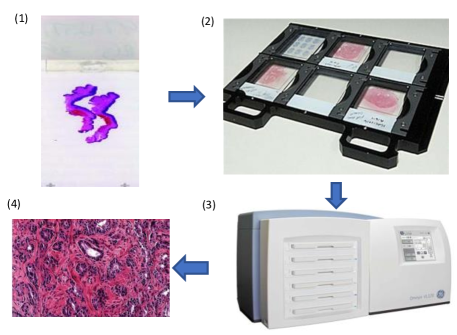
Figure 1: The workflow of the proposed whole-slide imaging. (1) is the glass slide Amin-2008-AWSI . (2) whole mount glass slides. (3) whole slide imaging scanner. (4) digital whole image Farahani-2015-WSIP .

As shown in Fig. 1, (1) is the pathologic biopsy, (2) is the whole mount glass slides, (3) is whole slide imaging scanner, (4) is the obtained WSIs. The optical microscope system is the essential part of the WSI scanner, especially the lens optics and the camera because it can determine the quality of the images. Charged coupled device (CCD) sensors on cameras that can convert analog signals into digital signals. There are two major methods of slide acquisition. One is area scanning, the other is line scanning. The area scanner moves on the sample block by block and section by section, that is, after stopping at each position to capture an image, it is repositioned to the next position. The line scanner is smooth and continuous movement and fast scanning Higgins-2015-ACDP . After choosing a range of interest on a slide, adjust focus, and scan the slide Amin-2008-AWSI . If WSI scanners have a Z-stacking facility (scan slides at different focal planes along the vertical Z-axis and stack images on top of each other to produce composite multi-planar images Farahani-2015-WSIP ), they can better center on particular areas of interest gabry-2014-WSIW . Owing to the images generated by the WSI systems are large, the visual field of a computer should be bigger than the visual field of a traditional microscope over four times Rojo-2006-CCCA .

With the accelerating development of science and technology, the WSI system has progressed rapidly. WSI offers higher quality and resolution images with annotation Pantanowitz-2011-RTCS . The scanner with fast scanning speed has improved image quality and reduced storage costs Janabi-2012-WSIA . The digital approach also can reduce the time of transporting glass slides and the risk of breakage and fading Ghaznavi-2013-DIPW  Camparo-2012UWSI  Webster-2014-WSIA . Moreover, the digital slides do not deteriorate over time saco-2016-CSWS .

WSI infuses into many fields such as E-education, virtual workshops, and pathology aspect. Now, there is a growing need for pathology to improve quality, patient safety, and diagnostic accuracy. These causes and economic pressures to consolidate and centralize diagnostic services Ghaznavi-2013-DIPW . Moreover, WSI can boost distinct pathology practices, so it is generally used in pathology Cornish-2012-WSIR . Digital pathology networks based on WSI systems can solve some difficult problems with pathology. For example, WSI can be explored by several observers from different areas at the same time. Discussions using WSI can save the time needed for transferring glass slides to distant places for attaining second minds and teleconsultation Janabi-2012-WSIA  Webster-2014-WSIA  Janabi-2012-WSIF . WSI equivalently broadens the scope of cytopathology where virtual slides are used for numerous intents like telecytology, quality activities (e.g. archiving and proficiency testing), and education (e.g. virtual atlases) gabry-2014-WSIW . It will also let pathologists become more efficient, precise, and creative at quantifying prognostic biomarkers like HER2/neu (c-erbB-2). But also, crucially, WSI develops CAD in combination with the continually developing computer artificial intelligence, big data, and cloud technology. Nowadays, WSI technology is very advance and offers the pathology community novel clinical, nonclinical, and research image-related applications Farahani-2015-WSIP .

1.2 The Development of WSI Analysis

The traditional pathological section analysis method requires specially trained pathologists to look for areas of interest under the microscope one by one, and then analyze and diagnose based on professional knowledge. Traditional manual analysis of pathological images has many drawbacks and problems. There are no quantitative indicators, so the qualitative analysis results cannot be reproduced Singh-2010-BCDC . Moreover, most doctors have tight working conditions, heavy workload, and time pressure. In this case, the human cognitive process is easily disturbed, leading to incomplete diagnosis and misdiagnosis Goggin-2007-CDSS . Although traditional slide analysis is accurate, it can be deeply personal. It is available for the same person to evaluate a slide one day and to get different conclusions the following week. Besides, the procedure is a challenging and time-consuming task Higgins-2015-ACDP . Therefore, CAD is a more efficient, accurate, and intuitive method.

The computer-aided reading slide can help pathologists improve diagnosis accuracy and detection rate and reduce the overall misdiagnosis rate. Moreover, the computer is not affected by fatigue and human error and provides better assistance to doctors Goggin-2007-CDSS  Fazal-2018-PPFR . It is also a valuable tool to reduce the workload of clinicians Lisboa-2006-UANN . While reducing pathologists’ workload and improving efficiency, it can also perform intuitive quantitative analysis of pathological conditions. These are better than manual reading slides. Computer-aided viewing of WSI is now rapidly developing. WSI provides the pathology field unique clinical, nonclinical, and analysis of image-related applications Farahani-2015-WSIP .

In recent years, the pathological WSI analysis performed by CAD doctors, it has been widely used in different cancer fields (ie, breast cancer, prostate cancer, gastric cancer, neuroblastoma). The scope of applications focuses on disease classification, early screening, tissue localization, and benign and malignant diagnosis. Common tasks with CAD include classification, segmentation, and detection.

For example, in the work of Huang-2017-AHGP , automatic detection and sequencing system based on Gleason pattern recognition is proposed for the automatic detection of high-grade prostate cancer. In the field of breast cancer, the work of Mehta-2018-LSBB makes the segmentation of WSI images of breast biopsy with biologically significant tissue markers. The study of Korbar-2017-DLCC trains a modified version of the residual network (ResNet) to classify different types of colorectal polyps on WSIs. At present, the development trend of computer-aided viewing of WSIs is shown in Fig. 2.

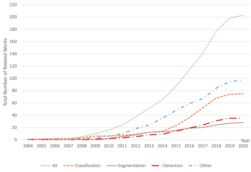
Figure 2: The development trend of computer-aided viewing of WSIs. The horizontal direction shows the time. The vertical direction shows the cumulative number of related works in each year.

As shown in Fig. 2, as the years are getting closer and closer, technology continues to advance. There are more and more cases of using computers to assist diagnosis. The number of cases in the three main applications of classification, segmentation, and detection has increased year by year. The number of cases in other applications are growing, such as retrieval Ma-2016-BHIR , localization Alomari-2009-LTHR . Beginning in 2008, CAD viewing WSI has helped pathologists begin to realize it significantly. Since 2014, there has been an increasing trend in the number of computer-aided pathologists diagnosed with WSI. Gradually by 2020, the growth rate of CAD has increased, reflecting the vigorous development of this technology.

Besides, to explain and clarify computer-aided pathologists’ work context in viewing WSI, an organization chart is shown in Fig. 3. The figure shows the general process of CAD and processing WSI. It shows seven important steps in the histopathology image analysis system, including data acquisition, image presentation, image preprocessing, feature extraction, data post-processing, classifier design, and system evaluation.

Figure 3: The organization chart of histopathology WSI analysis using computer-aided analysis approaches in this paper.

In Fig. 3, histopathological data initially obtained from the medical field, 2-D or 3-D digital microscopic images are first captured by various imaging equipment (e.g., optical microscopy), and then saved in a specific color space (e.g., Red, Green and Blue (RGB) color space). The 3rd step is the image pre-processing step, the properties of images are improved by dataset augmentation, segmentation, and so on, which is an importation preparation for the feature extraction step. In the next step, feature extraction is implemented, where the image can be represented by its attributes (shape, texture, and color features), or layout features (global and local features), or extraction style (manual or automatic). These feature extraction categories are not separate, but can be converted into other categories using appropriate methods. After that, the post-processing step takes the responsibility to enhance the extracted features, where filter, morphological processing, normalization are always used. Also, the classifier can be classified as shallow or deep according to its learning structure. Finally, various numerical and intuitive methods are used to evaluate the classification system, such as classification accuracy, classification error rate, sensitivity, and specificity. Besides, each step is not independent, but is closely connected with other steps through information feedback. Therefore, the entire CAD viewing WSI system is an organic whole C.Li-2016-CBMI .

1.3 Motivation of This Review

Now WSI technology has applications in many fields. For example, to perform preliminary diagnosis of surgical pathology, and perform intraoperative frozen section diagnosis through remote consultation huang-2018-TCFS  boyce-2017-AUVW , and seek expert advice without incurring international transportation costs or delays Boroujeni-2016-WSIH . WSI also provides advantages in tumor diagnosis, prognosis, and targeted therapy. It can also facilitate teachers and students in teaching Ghaznavi-2013-DIPW . Therefore, the research field of WSI analysis through CAD systems is significant. To the best of our knowledge, there exist some survey papers that summarize WSI analysis (e.g., the reviews in Pantanowitz-2011-RTCS ,  Gurcan-2009-HIAA ; Kothari-2013-PIIQ ; Veta-2014-BCHI ; Sharma-2015-ARGB ; Li-2018-LSRM ; Komura-2018-MLMH ; Chang-2019-AIIP ; Nichols-2019-MLAA ; Wang-2019-PIAU ; Dimitriou-2019-DLWS ; Kumar-2020-WSIP ). In the following part, the summary of survey papers related to the WSI analysis is presented.

The survey of Pantanowitz-2011-RTCS reviews the current status of WSI pathology, including supervision and verification, remote and routine pathological diagnosis, educational use, implementation issues, and cost-benefit analysis of WSI in routine clinical practice. However, this article only focuses on the application of CAD systems in WSI analysis. This review rarely mentions this, and only 12 references are about WSI.

The survey of Gurcan-2009-HIAA reviews the latest CAD techniques for digital histopathology. This article also briefly introduces new image analysis technologies developed and applied in the United States and Europe for some specific histopathology-related problems. More than 130 papers on CAD have been summarized and only three articles are about WSI.

The survey of Kothari-2013-PIIQ reviews the WSI informatics method of histopathology, related challenges and future research opportunities. However, this article reviews image quality control, feature extraction of image attributes captured at pixels, object, and semantic levels, image features for predictive modeling, and data and information visualization for diagnostic or predictive applications. It does not discuss the entire process of CAD and the viewing of WSI. More than 130 papers have been summarized. However, only three articles are about WSI.

The survey of Veta-2014-BCHI reviews the analysis methods of histopathological images of breast cancer, introduces the process of tissue preparation, staining, and slide digitization, and then discusses different image processing techniques and applications, from tissue staining analysis to CAD, and the prognosis of breast cancer patients. Although the histopathological images discussed in the article are WSIs, they are only about breast cancer and not comprehensive. More than 110 papers have been summarized. However, only four articles are about WSI.

The survey of Sharma-2015-ARGB provides a comprehensive overview of the graph-based methods explored so far in digital histopathology. More than 170 papers have been summarized. However, only four articles are about WSI.

The survey of Li-2018-LSRM reviews the latest methods of large-scale medical image analysis, which are mainly based on computer vision, machine learning, and information retrieval. Then, they comprehensively reviewed the algorithms and technologies related to the main processes in the pipeline, including feature representation, feature indexing, and search. However, WSI appears only in the sample dataset, and no actual analysis is performed. Of the more than 250 papers summarized in this paper, only three mention WSI.

The survey of Komura-2018-MLMH introduces the application of digital pathological image analysis using machine learning algorithms, solve some specific analysis problems, and propose possible solutions. However, there are only 11 articles related to WSI on the topics we are interested in. More than 120 papers have been summarized. But only 11 articles are about WSI.

The survey of Chang-2019-AIIP introduces the general situation of artificial intelligence, a brief history in the medical field and the latest developments in pathology, and the future prospects of pathology driven by it. This review only briefly mentions WSI in the part of the pathology application imaging and example datasets. Of the more than 70 papers summarized in this paper, only four mention WSI.

The survey of Kumar-2020-WSIP introduces the technical aspects of WSI, its application in diagnostic pathology, training and research, and its prospects. It highlights the benefits, limitations, and challenges of delaying the use of this technology in daily practice. But this article only focuses on computer-aided pathologists to view WSI and its application in diagnosis, which are not discussed in this review. Of the 50 references, 20 are about WSI.

From the existing review papers mentioned above, we can find that many researchers are concerned about the current status and development trend of WSI technology itself, and hundreds of related works have been systematically summarized and discussed in those review papers. However, all these survey papers use WSI format datasets as examples only, and do not aim to introduce the detailed introduction of computer-aided pathologists to review WSI technology. Therefore, we present this review paper to analyze all related works using CAD combined with WSI in the past few decades. This survey summarizes more than 210 related works from 2004 to 2020. The audience for this review is related researchers in the field of medical imaging and medical professionals.

1.4 Structure of This Review

This structure of this paper is as follows: Sec.  2 summarizes the related datasets and commonly used evaluation methods. Sec.  3 illustrates frequently used feature extraction methods. Sec.  4,  5, and  6 present the related work of segmentation, classification, and detection using WSI and CAD technology. After the overview of different works, the most frequently used approaches are analyzed in Sec. 7. Finally, Sec. 8 concludes this review with prospective future direction.

2 Datasets and Evaluation Methods

In this section, we have discussed some commonly used datasets and evaluation metrics for the classification, segmentation, and detection tasks.

2.1 Publicly Available Datasets about WSI

To better analyze the CAD using WSI technology, we have summarized some frequently used publicly available datasets in our study. Tab. 1 shows the necessary information of these datasets. Two of the most commonly used datasets are The Cancer Genome Atlas (TCGA) TCGA and the Camelyon datasets Litjens-2018-1HSS . Both datasets are often used for classification and detection. At the same time, we find two WSI datasets named TUPAC16 Veta-2019-PBTP and Kimia Path24 Babaie-2017-CRDP . TUPAC dataset is widely used, such as mitosis detection, prediction of breast tumor proliferation, automatic scoring (classification), and so on. Kimia Path24 is often used for classification and retrieval Babaie-2017-CRDP  Kumar-2018-DBFR . The basic information of the common datasets are shown in Table. 1.

Table 1: The basic information of the publicly available used datasets.

Databases	Year	Field	Number of images or or size
TCGA	2006	Cancer related	Over 470 TB
NLST Pathology Images	2009	Lung	Around 1250 H&E slides
BreakHis	2015	Breast cancer	9,109 microscopic images
TUPAC16	2016	Tumor mitosis	Around 821 H&E slides
Camelyon	2017	Breast cancer	Around 3TB
Kimia Path24	2017	Pathology Images	24 WSIs

2.1.1 TCGA database

TCGA is a project jointly launched by The National Cancer Institute (NCI) and the National Human Genome Research Institute (NHGRI) in 2006 TCGA . It contains clinical data, genome variation, mRNA expression, miRNA expression, methylation and other data of various human cancers (including subtypes of tumors). The database is designed to use high-throughput genomic analysis techniques to help people developing a better understanding of cancer and improve the ability to prevent, diagnose, and treatment Tomczak-2015-CGAI . While TCGA main work focuses on genomics and clinical data, it also accumulates a large number of WSIs in patient’s tissue. Since WSI datasets are much larger than other datasets, to facilitate viewing, David et al. Gutman-2013-CDSA proposes an integrated network platform named Cancer Digital Slide Archive (CDSA) to accommodate all WSI in TCGA. Since the dataset contains many types of cancers, it has a wide range of uses. Fig. 4 below is an example of WSIs in an adrenal cortical carcinoma in the TCGA database.

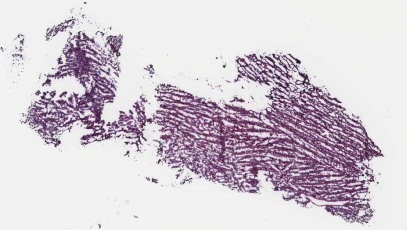
Figure 4: An example of WSI in an adrenal cortical carcinoma in the TCGA database TCGA .

2.1.2 Camelyon Database

The Camelyon Challenge is hosted by International Symposium on Biomedical Imaging (ISBI) Litjens-2018-1HSS . The whole competition dataset (Camelyon16, Camelyon17 ) are derived from sentinel lymph nodes of breast cancer patients contains WSIs of Hematoxylin and Eosin (H&E) stained node sections Bejnordi-2017-DADL Bandi-2018-DIMC . Therefore, the Camelyon dataset is suitable for the automatic detection and classification of breast cancer in WSI. The data of Camelyon16 are from the Radboud University Medical Centre and the University of Utrecht Medical Centre. The Camelyon16 dataset is composed of 170 phase I lymph node WSIs (100 normals and 70 metastatics) and 100 Phase II WSIs (60 normals and 40 metastatics), and the test dataset consisted of 130 WSIs from two universities. The Camelyon16 dataset is used as training values for the evaluation of Camelyon17. Fig. 5 is a pathological picture of a lymph node in Camelyon. The left side belongs to normal cell tissue, and the right cell has been swallowed and occupied by cancer cells.

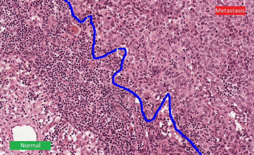
Figure 5: A pathological image of a lymph node in Camelyon Litjens-2018-1HSS . The left side belongs to normal cell tissue, and the right cell has been swallowed and occupied by cancer cells.

2.1.3 TUPAC16 Database

The TUPAC16 challenge is held in the context of the MICCAI Veta-2019-PBTP . TUPAC16 main challenge dataset consists of 821 TCGA WSIs with two types of tumor proliferation data. 500 for training, 321 for testing. In addition to the main challenge dataset, there are two secondary datasets (area of interest and mitotic detection). The area of interest auxiliary dataset contains 148 cases that are randomly selected from the training dataset. The mitotic test dataset consisted of WSIs of 73 breast cancer cases from three pathological centers. Of the 73 cases, 23 are AMIDA13 challenge Veta-2015-AAMD . The remaining 50 cases previously used to assess the interobserver agreement for mitosis counting are from two other pathology centers in the Netherlands. So the dataset is mainly used for automatic detection of tumor mitosis or other regions of interest(ROI). Fig. 6 shows some examples of mitosis maps in H&E breast cancer slices, with green arrows marking mitosis.

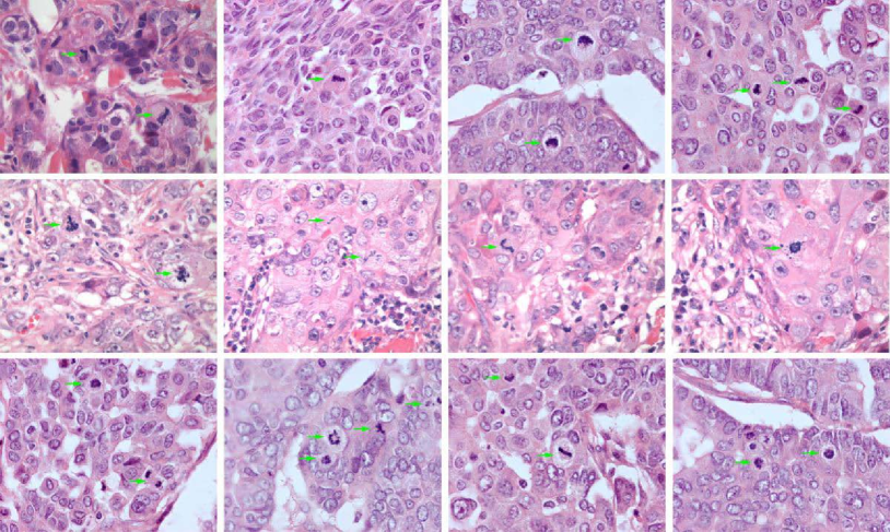
Figure 6: Some examples of mitosis diagrams in H&E breast cancer slices in the TUPAC16 Veta-2019-PBTP , with green arrows marking mitosis.

2.1.4 Kimia Path24 Database

This dataset is consciously and manually selected from 350 WSIs from different body parts so that the 24 WSIs clearly represented different texture patterns. So this dataset is more like a computer vision dataset (as opposed to a pathology dataset) because visual attention is spent on the diversity of patterns rather than on anatomy and malignancy Babaie-2017-CRDP . Therefore, this dataset is mainly used for classification and retrieval of histopathological images. The 24 WSIs thumbnails in this dataset are shown in Fig. 7.

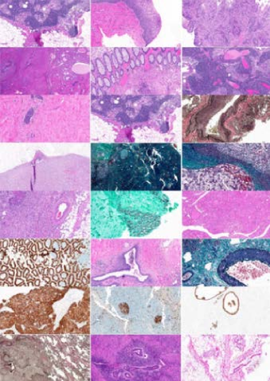
Figure 7: 24 WSIs thumbnails in Kimia Path24 database Babaie-2017-CRDP .

2.2 Evaluation Method

This subsection introduces the evaluation methods of classification, segmentation, and detection algorithms and related formulas.

2.2.1 Basic Evaluation Indexs

The confusion matrix is used to observe the performance of the model in each category, and the probability of each category can be calculated. The specific style of the confusion matrix is shown in Tab. 2.

Table 2: Confusion matrix of basic evaluation indexs.

Data Class	Classified as Pos	Classified as Neg
Pos	True Positive(TP)	False Negative(FN)
Neg	False positive(FP)	True Negative(TN)

According to the confusion matrix, the True Positive Rate (TPR) can be defined as TP/(TP + FN), which represents the proportion of the actual positive instances in all positive instances of the positive class predicted by the classifier, the False Postive Rate (FPR) can be defined as FP/(FP+TN), which represents the proportion of the actual negative instances in all negative instances of the positive class predicted by the classifier. It can be seen that the mathematical expressions of the following evaluation metrics are shown in Table. 3 Sokolova-2009-SAPM .

Table 3: Evaluation metrics. Acc, P, R, Se, Sp and F1 denote accuracy, precision, recall, sensitivity, specificity and F1 score, respectively.

Assessments	Formula	Assessments	Formula
Acc	$\frac{TP+TN}{TP+TN+FP+FN}$	Se	$\frac{TP}{TP+FN}$
P	$\frac{TP}{TP+FP}$	Sp	$\frac{TN}{TN+FP}$
R	$\frac{TP}{TP+FN}$	F1	$2\texttimes\frac{P\texttimes R}{P+R}$

2.2.2 Evaluation of Segmentation Methods

Image segmentation Haralick-1985-IST is the segmentation of images with existing targets and precise boundaries. The commonly used indicators are accuracy, precision, recall, F-measure, sensitivity, and specificity. These metrics we have discussed in Sec. 2.2.1 and their mathematical expressions are given Tab. 2. Dice co-efficient (D) and Jaccard index (J) are popular segmentation evaluation indexes in recent years. Dice co-efficient (D) represents the ratio of the area intersected by two individuals to the total area, that is, the similarity between ground truth and the segmentation result graph. If the segmentation is perfect, the value is 1. Then, if S stands for the segmentation result graph and G stands for ground truth, the expression of Dice co-efficient (D) is given in Eq. (1).

$$D(S,G)=\frac{2|A\cap G|}{|A|+|G|}$$ (1)

Jaccard Index (J) represents the intersection ratio of two individuals, which is similar to Dice co-efficient. The formula is given in Eq. (2).

$$J(S,G)=\frac{|A\cap G|}{|A\cup G|}$$ (2)

2.2.3 Evaluation of Classification Methods

Classification Kamavisdar-2013SICA is the operation of determining the properties of objects in the image. In the field of digital histopathology we studied, some are the classification of cancer Petushi-2006-LSCH , some are the operation of selecting ROI Swiderska-2015-TMMH , and some are the identification of cancer regions Doyle-2010-BBMC . The purpose of classification is achieved by the constructed classifier. The performance indicators used to evaluate these classifiers are critical to the final results. Accuracy is the most commonly used indicators to evaluate classifiers. Precision, recall, sensitivity, specificity, and F1 score are widely used to evaluate classifiers. Accuracy,precision, recall, F-measure, sensitivity, and specificity we have discussed in Sec. 2.2.1 and their mathematical expressions are given in Tab. 2. With the continuous improvement of classification requirements in practical applications, ROC (Receiver Operating Characteristic), AUC (Area Under ROC Curve), a non-traditional measurement standard, have emerged. ROC is a curve drawn on a two-dimensional plane with FPR as the abscissa and TPR as the ordinate. It can reflect the sensitivity and specificity of the continuous variables as a comprehensive indicator. It can also solve the problem of class imbalance in the actual dataset. AUC quantifies the area under the ROC curve into a numerical value to make the results more intuitive.

2.2.4 Evaluation of Detection Methods

Detection Pal-1993-RIST is another common task in analyzing histopathological WSIs. Detection is not only to determine the attributes of the region identified in WSI, but also to identify and obtain more detailed results. Because of the similarity between testing and classification, most of the evaluation indexes are the same as the classification, including accuracy, precision, recall, F-measure, sensitivity, and specificity that we have discussed in Sec. 2.2.1. However, in WSI detection, it is difficult to locate, determine and quantify multiple lesions. Therefore, FROC (Free Receiver Operating Characteristic Curve) Egan-1961-OCSD is proposed to evaluate the detection results. FROC curve is a small variation of the ROC curve. It is a curve drawn on a two-dimensional plane with FP as the horizontal coordinate and TPR as the vertical coordinate. This allows the detection of multiple lesion areas on a single WSI.

2.3 Summary

According to the review above, we can see that the commonly used public datasets are TCGA, TUPAC16, and Kimia Path24 for the classification, segmentation, and detection of histopathological images using the combination of WSI technology and CAD with the brief introduction. Also, the evaluation indicators of these three tasks. The basic commonly used evaluation indicators are accuracy, precision, recall, sensitivity, and specificity. In terms of classification, there are comprehensive indicators such as AUC. Dice co-efficient and Jaccard index in segmentation indicators have become popular in recent years, and FROC in detection indicators can be used for positioning, qualitative and quantitative analysis of multiple lesions.

3 Feature Extraction

Traditional image feature extraction is generally divided into three steps: preprocessing, feature extraction, and feature processing. Then using machine learning methods to segment and classify the features. The purpose of preprocessing is to eliminate interference factors and highlight characteristic information. The main methods are: image standardization Shen-2003-PSBM (adjust the image size); image normalization Khan-2014-NMAS (adjust the image center of gravity to 0). The main purpose of feature processing is to eliminate features with a small amount of information and reduce the amount of calculation. The common feature processing method is principal components analysis Jhajharia-2016-NNBB .

Among them, feature extraction is a crucial step. Converting input data into a set of features is called feature extraction Ping-2013-RIFE . The main goal of feature extraction is to obtain the most relevant information from the original data and represent the information in a lower-dimensional space Kumar-2014-DRFE . Therefore, in this section, we mainly summarize the features extracted in WSI for CAD. The types of extracted features are shown in Fig. 8.

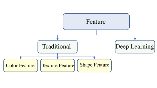
Figure 8: The types of feature extraction methods.

3.1 Traditional Feature Extraction

In the process of segmentation, classification, or detection combined with CAD and WSI technology, the commonly used extracted features include color features, texture features and shape features.

3.1.1 Color Featur Extraction

Color is an important feature, which is widely used for image representation Kodituwakku-2004-CCFI . The color of an image is invariant to rotation, translation, or scaling. Color characteristics are defined according to a specific color space or model Ping-2013-RIFE . Many color spaces are used in the literature such as RGB Roullier-2010-GMRS , HSV ((Hue Saturation Value)) Mercan-2016-LDRR , and LAB Mercan-2016-MIML . Common color features include color histograms, color moments, and color coherence vector(CCV) Pass-1997-CIUC . Among the papers we summarized, 24 papers used color features Kong-2009-CAEN ; Roullier-2010-GMRS ; Samsi-2012-ECFA ; Kothari-2012-BIMP ; Akakin-2012-CBMI ; Collins-2013-AMAU ; Nayak-2013-CTHS ; Veta-2013-DMFB ; Kothari-2013-ETFA ; Homeyer-2013-PQNH ; Hiary-2013-SLWS ; Bautista-2014-CSWS ; Mercan-2014-LDRR ; Yeh-2014-MSDP ; Litjens-2015-ADPC ; Weingant-2015-EPTC ; Li-2015-FRID ; Mercan-2016-LDRR ; Barker-2016-ACBT ; Mercan-2016-MIML ; Brieu-2016-SSMS ; Mercan-2017-MIML ; Cruz-2018-HTAS ; Morkunas-2018-MLBC .

RGB-based Color Features

We have found 12 studies that utilized RGB feature extraction technique Kong-2009-CAEN ; Roullier-2010-GMRS ; Akakin-2012-CBMI ; Collins-2013-AMAU ; Veta-2013-DMFB ; Homeyer-2013-PQNH ; Hiary-2013-SLWS ; Bautista-2014-CSWS ; Yeh-2014-MSDP ; Litjens-2015-ADPC ; Cruz-2018-HTAS ; Morkunas-2018-MLBC .

The color features extracted by  Kong-2009-CAEN are combined with the color and entropy information extracted from the RGB image channel. In Roullier-2010-GMRS , the vector extracted with the RGB feature indicates that the feature vector of each pixel is the local entropy of the red-green difference calculated in the square neighborhood around the pixel. In Akakin-2012-CBMI , the mean and standard deviations are calculated as first-order and second-order statistical features from the three RGB channels, and there are six features. The author in  Collins-2013-AMAU extracts core RGB features. The color features of Veta-2013-DMFB are described by the average, standard deviation, minimum and maximum values of the three color channels in the RGB color space in the candidate area and two other areas. In Fig. 10 an example of features distribution image showing the spatial distribution of the cell nuclear diameter in Yeh-2014-MSDP . The work of Homeyer-2013-PQNH extracts the PVS function of each R, G, and B channel (8 pixel value statistics). PVS is composed of the minimum, maximum, sum, average, and standard deviation of the constituent pixels, and the lower quartile, median and upper quartile are composed of values in a specific color channel. Fig. 9 shows the RGB feature extraction and classification in Homeyer-2013-PQNH .

Figure 9: An image after RGB feature extraction and classification in Homeyer-2013-PQNH . This figure corresponds to Fig.2 (2) in the original paper.

The author in  Hiary-2013-SLWS extracts the variance in each color channel of RGB: s2R, s2G, s2B, the variance (maximum value) between the peaks of each color channel s2. The work of Bautista-2014-CSWS uses color saturation and RGB color. Yeh-2014-MSDP extracts color features from the RGB channels. Fig. 10 shows an example of feature distribution of the cell nuclear in diameter Yeh-2014-MSDP .

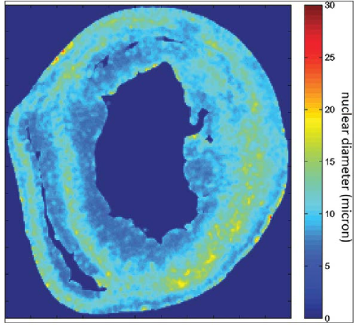
Figure 10: An example of feature distribution image in Yeh-2014-MSDP . This figure corresponds to Fig.10 in the original paper.

The author in  Litjens-2015-ADPC extracts RGB histogram, and overlay features. Cruz-2018-HTAS extracts the first-order statistics of 14 color channels, and the color histogram of each RGB channel is 8×38 bin histogram. In Morkunas-2018-MLBC , for each 2D superpixel (for example, grayscale superpixel), two statistics are calculated of mean and standard deviation of the pixel value. For 3D superpixels (such as RGB superpixels), eight statistics are calculated the mean and standard deviation of the pixel value for each color channel and each RGB superpixel, then this as a color function.

HSV-based Color Features

There are four papers on color feature extraction based on HSV Samsi-2012-ECFA ; Akakin-2012-CBMI ; Homeyer-2013-PQNH ; Bautista-2014-CSWS .

In Samsi-2012-ECFA , the extracted color feature is the hue channel converted from the HSV color space of the original image. In Akakin-2012-CBMI , from the three HSV channels, the average and standard deviation are calculated as first-order and second-order statistical features, and a total of six features are extracted. Homeyer-2013-PQNH extracts the PVS function of each H, S and V channel. Bautista-2014-CSWS uses color saturation and value and RGB color as a function in HSV color space.

LAB-based Color Features

There are five papers on color feature extraction based on LAB Kong-2009-CAEN ; Akakin-2012-CBMI ; Mercan-2014-LDRR ; Mercan-2016-LDRR ; Mercan-2017-MIML .

In Kong-2009-CAEN , the extracted color features are composed of color and entropy information extracted from LAB image channels. In Akakin-2012-CBMI , from the three channels of CIELAB, the average and standard deviation are calculated as first-order and second-order statistical features, and a total of six features are extracted. Mercan-2014-LDRR extracted the color histogram calculated in LAB space. Fig. 11 shows the color histogram mentioned in the paper. Cutting the WSI into a patch is a normal operation in the image processing process. (a,b,c,f,g,h) in Fig. 11 are the image blocks after the WSI slice.

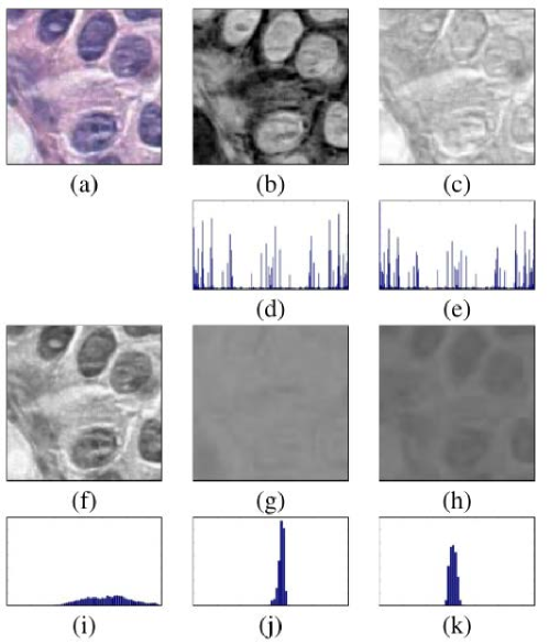
Figure 11: (a) Original $120\times 120$ pixel patch, (b) deconvolved color channel that shows good contrast for nuclei dyed with haematoxylin, (c) deconvolved color channel that shows good contrast for eosin dye, (d) LBP histogram calculated on haematoxylin channel, (e) LBP histogram calculated on eosin channel,(f, g, h) L, a, and b channels of the image in LAB color space,(i, j, k) color histograms of L, A and B channels. At the end, LBP histograms on two channels are concatenated to produce the first set of features, color histograms on LAB channels are concatenated to produce the second set of features. These figure are from Mercan-2014-LDRR . This figure corresponds to Fig.3 in the original paper.

The color feature of  Mercan-2016-LDRR is the LAB histogram of the color. Mercan-2017-MIML uses the color histogram calculated for each channel in the CIE-Lab space as the color feature.

Others Color Features

Other papers related to color feature extraction total of six Nayak-2013-CTHS ; Kothari-2013-ETFA ; Hiary-2013-SLWS ; Weingant-2015-EPTC ; Li-2015-FRID ; Barker-2016-ACBT ; Brieu-2016-SSMS .

Nayak-2013-CTHS and Kothari-2013-ETFA extract the color information in WSIs as features. Hiary-2013-SLWS extracts the average value of the variance, saturation, brightness of HSI and the hue value of the color model $\mu$. Weingant-2015-EPTC extracts the color channel histogram as the color feature. Li-2015-FRID extracts the histogram of the three-channel HSD color model as color features. Brieu-2016-SSMS extracts the color information in WSI as features. Barker-2016-ACBT extracts rough color features. The rough feature is the use of feature analysis of the diversity of rough areas in WSI to roughly characterize their shape, color, and texture. The fine feature refers to the more comprehensive image features extracted from the slice to express deeper features. The feature histogram extracts in Barker-2016-ACBT is shown in Fig. 12.

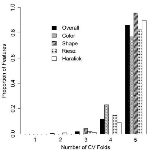
Figure 12: Histogram distribution of features used in Elastic Net models, showing the number of models in which features of a given class appear. The number of features is normalized based on the total number of features represented for each class. Bar patterns represent the feature class. Most features for each class appear in all, or nearly all models, as expected if they have diagnostic value. This figure is from  Barker-2016-ACBT . This figure corresponds to Fig.7 in the original paper.

From the above review, we can see that in terms of color feature extraction, the RGB color features are used most frequently, focusing on the period from 2009 to 2018. Then HSV color feature and LAB (CIE-LAB) color feature. The dates are 2012 to 2014 and 2009 to 2017. In other papers, HSI and HSD color models are used as color characteristics.

3.1.2 Texture Featur Extraction

The texture feature describes the surface properties of the object corresponding to the image or image area. Unlike the color feature, the texture feature is not based on the feature of pixels. It needs to be calculated in the area containing multiple pixels. Texture feature is an effective method when judging images with large differences in thickness and density. However, when the thickness, density, feature are easy to distinguish between the information. However, difficult for the usual texture features to accurately reflect the differences between the textures with different human visual perception.

Commonly used texture information description methods are: statistical methods ( such as gray-level co-occurrence matrix (GLCM) Mohanaiah-2013-ITFE ), geometric methods (such as voronoi checkerboard feature method Tuceryan-1990-TSUV ), model methods (such as random fields Chellappa-1985-CTUG ), and signal processing methods (such as wavelet transform Pichler-1996-CTFE ). Among the papers we summarized, 57 papers used texture features Diamond-2004-UMCT ; Petushi-2006-LSCH ; Sertel-2008-CAPN ; Sertel-2009-CCCS ; Kong-2009-CAEN ; Sertel-2009-CPNW ; Roullier-2010-MEBC ; Doyle-2010-BBMC ; Difranco-2011-ESWS ; Kong-2011-IMAG ; Roullier-2011-MRGA ; Grunkin-2011-PCIA ; Nguyen-2011-PCDF ; Akakin-2012-CBMI ; Sharma-2012-DSHI ; Nayak-2013-CTHS ; Jiao-2013-CCDU ; Veta-2013-DMFB ; Kothari-2013-ETFA ; Kong-2013-MBMA ; Homeyer-2013-PQNH ; Hiary-2013-SLWS ; Mercan-2014-LDRR ; Apou-2014-FSTC ; Bejnordi-2015-MSSC ; Sharma-2015-ABND ; Swiderska-2015-CMSA ; Weingant-2015-EPTC ; Li-2015-FRID ; Zhang-2015-FGHI ; Cooper-2015-NGPA ; Apou-2015-SWSI ; Peikari-2015-TDRR ; Mercan-2016-LDRR ; Barker-2016-ACBT ; Bejnordi-2016-ADDW ; Zhao-2016-AGEW ; Harder-2016-CFCG ; Shirinifard-2016-DPAU ; Gadermayr-2016-DACC ; Leo-2016-ESHF ; Mercan-2016-MIML ; Brieu-2016-SSMS ; Saltz-2017-CSSG ; Mercan-2017-MIML ; Hu-2017-DLBC ; Bejnordi-2017-DADL ; Valkonen-2017-MDWS ; Mirschl-2018-DLCI ; Xu-2018-AACM ; Yoshida-2018-AHCWG ; Han-2018-ACDL ; Morkunas-2018-MLBC ; Simon-2018-MRLF ; Klimov-2019-WSIB .

Local Binary Pattern-based Texture Features

There are 14 papers on texture feature extraction based on local binary pattern (LBP) Sertel-2008-CAPN ; Sertel-2009-CPNW ; Roullier-2010-MEBC ; Roullier-2011-MRGA ; Homeyer-2013-PQNH ; Mercan-2014-LDRR ; Bejnordi-2015-MSSC ; Mercan-2016-LDRR ; Mercan-2016-MIML ; Gadermayr-2016-DACC ; Babaie-2017-CRDP ; Mercan-2017-MIML ; Bejnordi-2017-DADL ; Simon-2018-MRLF . In Sertel-2008-CAPN ; Sertel-2009-CPNW ; Roullier-2010-MEBC ; Roullier-2011-MRGA ; Homeyer-2013-PQNH ; Bejnordi-2015-MSSC ; Mercan-2016-LDRR ; Mercan-2016-MIML ; Babaie-2017-CRDP ; Mercan-2017-MIML , texture histograms of LBP features are extracted as texture features. Fig. 13 shows the calculation of the LBP feature of a given pixel in Sertel-2009-CPNW .

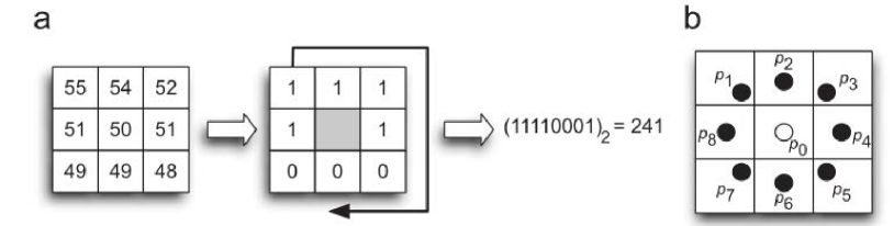
Figure 13: (a) The conventional LBP operator; (b) Circular pattern used to compute rotation invariant uniform patterns. This figure corresponds to Fig.5 in  Sertel-2009-CPNW .

Texture features compute using LBP for small image patches are extracted from Mercan-2014-LDRR . In Gadermayr-2016-DACC , multi-resolution LBP is extracted as the texture feature. In Bejnordi-2017-DADL , different structural texture features are extracted, including LBP features. In  Simon-2018-MRLF , LBP, MRC LBP feature are extracted as texture features.

Haralick-based Texture Features

Five papers involve texture feature extraction based on Haralick Diamond-2004-UMCT ; Sertel-2008-CAPN ; Kong-2009-CAEN ; Leo-2016-ESHF ; Hu-2017-DLBC . In Diamond-2004-UMCT , 4 Haralick features are the most suitable for discriminating stroma from PCA. Haralick features are extracted as texture features in Sertel-2008-CAPN ; Kong-2009-CAEN ; Leo-2016-ESHF . In Hu-2017-DLBC , extracts 57 subcellular location features, including Haralick texture features and DNA overlapping the features (experiments). The experimental images in Leo-2016-ESHF and the extracted haralick features are shown in Fig. 14.

Figure 14: (a, b) is the experimental image, (c, d) is the Haralick intensity texture. This figure corresponds to Fig.2 in Leo-2016-ESHF .

GLCM-based Texture Features

Eight papers involve texture feature extraction based on GLCM Sertel-2009-CCCS ; Doyle-2010-BBMC ; Difranco-2011-ESWS ; Jiao-2013-CCDU ; Hiary-2013-SLWS ; Weingant-2015-EPTC ; Bejnordi-2016-ADDW ; Morkunas-2018-MLBC .

In Sertel-2009-CCCS , the extraction of the mean and variance of the range of values within the local neighborhoods and entropy and homogeneity of co-occurrence histograms as texture features. Co-occurrence features are extracted as texture features from Doyle-2010-BBMC and Difranco-2011-ESWS . 16 features such as mean and variance are combined to form a group of 18 features Jiao-2013-CCDU . In Hiary-2013-SLWS , co-occurrence matrix, correlation, and energy are extracted as texture features. In Weingant-2015-EPTC , GLCM features are extracted. In Bejnordi-2016-ADDW , co-occurrence matrix statistics are extracted for each hyperpixel. In Morkunas-2018-MLBC , 2D hyper-pixel texture is obtained by using the spatial grayscale symbiosis matrix and 1px displacement vector of 3D hyper-pixel. From the co-occurrence matrix, the second moment of angle, contrast, correlation, sum of squares, deficit moment, average, sum variance, sum entropy, entropy, difference variance, difference entropy, and correlation information measures 1 and 2 are calculated. The average value of the 13 parameters obtained is the characteristic descriptor.

Filter and Scale-invariant Feature Transform(SIFT)-based Texture Features

There are five related papers on filter and SIFT based texture feature extraction Nguyen-2011-PCDF ; Peikari-2015-TDRR ; Bejnordi-2016-ADDW ; Bejnordi-2017-DADL ; Valkonen-2017-MDWS .

In Nguyen-2011-PCDF , first-order statistics, second-order statistics, and gabor filter features are used as texture features. In Peikari-2015-TDRR , a Gauss-like texture filter is applied to extract texture features. Fig. 15 shows the uniform distribution of histogram filter response in Peikari-2015-TDRR .

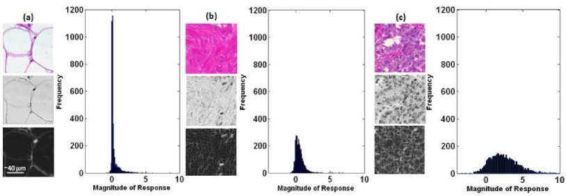
Figure 15: Patches of three different tissue types (in RGB) corresponding to (a) fat, (b) stroma, and (c) epithelial cells -top- along with their normalized luminance channel images (after converting them from RGB to LAB) -middle-, and maximal filter responses after convolving Gaussian-like filters at all directions of onescale (($\sigma$x, $\sigma$y) = (1,3)) -bottom-, and plot showing their histogram of filter response magnitudes. This figure corresponds to Fig.3 in Peikari-2015-TDRR .

In Bejnordi-2016-ADDW , the gray histogram statistics extracted from the filter bank response for each hyperpixel. Different structural texture features, such as SIFT features, are extracted from Bejnordi-2017-DADL . The vlfeat implementation of MSER (Maximally Stable Extremal Regions) and SIFT is used by extracting from Valkonen-2017-MDWS .

Others Texture Features

There are a total of 24 related papers based on the extraction of other texture features Petushi-2006-LSCH ; Kong-2011-IMAG ; Grunkin-2011-PCIA ; Akakin-2012-CBMI ; Sharma-2012-DSHI ; Nayak-2013-CTHS ; Kothari-2013-ETFA ; Kong-2013-MBMA ; Apou-2014-FSTC ; Swiderska-2015-CMSA ; Li-2015-FRID ; Zhang-2015-FGHI ; Cooper-2015-NGPA ; Apou-2015-SWSI ; Barker-2016-ACBT ; Shirinifard-2016-DPAU ; Gadermayr-2016-DACC ; Brieu-2016-SSMS ; Mirschl-2018-DLCI ; Xu-2018-AACM ; Yoshida-2018-AHCWG ; Han-2018-ACDL ; Klimov-2019-WSIB . Texture Parameters: DNM1, DNM2,DNM3, DNM1-2, DNM1-3, DNM2-3, DNM2-2-3, DT,DN are extracted from Petushi-2006-LSCH . The feature vector extracted in Petushi-2006-LSCH is shown in Fig. 16.

Figure 16: Tissue microtextures identified using image processing. The first three columns show examples of cell nuclei belonging to nucleus morphology categories NM1, NM2, and NM3, respectively. The textures identified as ECM and AT represent, respectively the collagen-rich stroma, and fat and tissue-devoid regions of the slide. This figure corresponds to Fig.2 in Petushi-2006-LSCH .

The texture is applied to the cytoplasmic region around the nucleus in Kong-2011-IMAG . In Grunkin-2011-PCIA , texture features are used to identify areas with high or low intensity variability in the image. Average, standard deviation, contrast, correlation, energy, entropy, and uniformity are extracted from Akakin-2012-CBMI as texture features. Texton-based texture is extracted from Sharma-2012-DSHI . In Nayak-2013-CTHS , texture information is used as feature. In  Kothari-2013-ETFA , quantitative image features are extracted to capture its texture. Nuclear texture features are extracted from the chromatin content and distribution in Kong-2013-MBMA . Each area is tagged according to its texture description in Apou-2014-FSTC . Intensity on the basis of histograms of the sum and difference images are extracted as texture features in Swiderska-2015-CMSA . In Li-2015-FRID , texture features are extracted for classification. In Zhang-2015-FGHI , the texture feature is extracted from the cell image and compressed into a binary code. These compressed features are stored in a hash table that allows constant time access across many images. In Cooper-2015-NGPA , the texture features of each nucleus are extracted. In Apou-2015-SWSI , the area is rendered using a manually positioned texture unit. The Fig. 17 shows the procedural structure and texture rendered in Apou-2015-SWSI .

Figure 17: Procedural structure and texture: (a) Procedural 3D model of a lobular epithelial layer. (b) Slice of (a) showing 2D lobular patterns. (c) Procedural cell rendering (random layout, arbitrary colors). This figure corresponds to Fig.5 in Apou-2015-SWSI .

Barker-2016-ACBT , use the riesz texture features. The texture features of slides stained with Ki67 are extracted from Shirinifard-2016-DPAU . The author of  Gadermayr-2016-DACC extracts Histograms of Oriented Gradients (HOG), and Fisher Vectors (FV) as texture features. The kernel texture features are extracted in Brieu-2016-SSMS and Saltz-2017-CSSG . In Mirschl-2018-DLCI , texture features are extracted from the ROI. In Xu-2018-AACM , the texture of the subregion is extracted for statistical analysis and classification. In Yoshida-2018-AHCWG , the standard deviation (variance) within the area defined by the contour is used as the texture feature. Han-2018-ACDL , extract the first-and second-order texture features. A total of 166 texture features are extracted from the convolved hematoxylin (nuclear staining) channel in Klimov-2019-WSIB .

3.1.3 Shape Featur Extraction

The shape feature is just what the name suggests. Under normal circumstances, there are two ways to represent shape features. One is contour features, and the other is regional features. The contour feature of the image is mainly for the outer boundary of the image, and the regional feature of the image is related to the entire shape area Zhang-2004-RSRD . Commonly used shape feature extraction methods include boundary feature method (such as hough transform method Philip-1994-FHSF ), geometric parameter method (such as moment, area, circumference Huang-1997-OLSV ), fourier descriptors Zhang-2012-MFDS , and other methods. There are 15 papers that use shape features among the papers we have summarized Diamond-2004-UMCT ; Kong-2011-IMAG ; Grunkin-2011-PCIA ; Lu-2012-ASAE ; Kothari-2012-BIMP ; Veta-2012-PVAE ; Lopez-2013-ABDM ; Collins-2013-AMAU ; Veta-2013-DMFB ; Kothari-2013-ETFA ; Kong-2013-MBMA ; Cooper-2015-NGPA ; Barker-2016-ACBT ; Saltz-2017-CSSG ; Xu-2018-AACM .

Basic Geometric Parameter-based Shape Feature

Among the papers that used shape feature extraction, seven papers extracted basic geometric shape features Lu-2012-ASAE ; Kothari-2012-BIMP ; Veta-2012-PVAE ; Collins-2013-AMAU ; Veta-2013-DMFB ; Kong-2013-MBMA ; Grunkin-2011-PCIA . The feature extraction steps in six of the papers are all used to classify, segment, or detect the task before it is used to better represent the image. In Lu-2012-ASAE , the major axis length to minor axis length ratio of a best-fit ellipse is extracted as the shape feature to eliminate false regions. In Kothari-2012-BIMP , eosinophilic-object shape features (pixel area, elliptical area, major-minor axes lengths, eccentricity, boundary fractal, bending energy, convex hull area, solidity, perimeter, and count) are extracted. The author in  Veta-2012-PVAE extracts two morphometric features, the mean nuclear area and standard deviation of the nuclear area, using a fully automatic segmentation method on WSIs. The author in  Collins-2013-AMAU extracts basic morphologic features and calculates its odds ratio for malignant tumors. The author in  Veta-2013-DMFB extracts compactness, eccentricity, firmness, and sphericity as shape features. The author in  Kong-2013-MBMA extractes perimeter, eccentricity, circularity, major axis length, minor axis length as geometric shape feature. Fig. 18 shows the morphological characteristic spectrum of the image in Kong-2013-MBMA . The seventh paper Grunkin-2011-PCIA is the morphological feature extraction for post-processing.

Figure 18: Image analysis enables the reliable and objective characterization of tissues through a process of image normalization, image segmentation, and feature extraction.

Other Shape Features

In the early days, some existing library functions and third-party existing functions were usually used to directly extract features. In Diamond-2004-UMCT ; Kong-2011-IMAG ; Saltz-2017-CSSG ; Xu-2018-AACM , the nuclear morphological features of the nuclei in WSI are extracted as the shape features of the images.

Over time, many other advanced extraction methods have emerged. There are also four papers on other shape feature extraction Lopez-2013-ABDM ; Kothari-2013-ETFA ; Cooper-2015-NGPA ; Barker-2016-ACBT . Lopez-2013-ABDM extractes multiple sharpness features. In Kothari-2013-ETFA , the author extractes 461 quantitative image features capturing the texture, color, shape, and topological properties of a histopathological image. Cooper-2015-NGPA extracts precise quantitative morphometric features. There are shape features in the core feature group extracted by Barker-2016-ACBT .

3.2 Deep Learning Feature Extraction

Convolutional Neural Network (CNN) is widely used to extract the deep learning features in various WSI analysis tasks. In the papers, a total of 53 papers used CNN for deep learning feature extraction Puerto-2016-DPAW ; Sharma-2016-DCNN ; Wang-2016-DLIM ; Geccer-2016-DCBC ; Sirinukunwattana-2016-LSDL ; Hou-2016-PCNN ; Sheikhzadeh-2016-ALMB ; Cruz-2017-ARIB ; Wollmann-2017-AGBC ; Araujo-2017-CBCH ; Bejnordi-2017-CASC ; Sharma-2017-DCNN ; Korbar-2017-DLCC ; Jimenez-2017-DMCR ; Xu-2017-LSTH ; Korbar-2017-LUHD ; Ghosh-2017-SLCA ; Das-2017-CHWS ; Cui-2018-DLAO ; Zanjani-2018-CDHW ; Courtiol-2018-CDLH ; Kumar-2018-DBFR ; Bychkov-2018-DLTA ; Gecer-2018-DCCW ; Ren-2018-DPCP ; Tellez-2018-GWSI ; Sirinukunwattana-2018-IWSS ; Kwok-2018-MCBC ; Das-2018-MILD ; Lin-2018-SFDS ; Campanella-2018-TSDM ; Jiang-2018-TMDD ; Wang-2018-WSLW ; Shou-2018-WSIC ; Tellez-2018-WSMD ; Bertram-2019-LSDM ; Li-2019-AMRM ; Liu-2019-AIBC ; Campanella-2019-CGCP ; Yue-2019-CCOP ; Maksoud-2019-CCOR ; Bilaloglu-2019-EPCW ; Lin-2019-FSFD ; Yu-2019-LSGC ; Sanghvi-2019-PAIA ; Wang-2019-RRMI ; Kohlberger-2019-WSIF ; Xu-2019-MTPW ; Chen-2020-ITWS ; Sornapudi-2020-CWSH ; Pantanowitz-2020-AIAP .

The basic configuration of CNN is the convolutional layer, pooling layer and fully connected layer  Rahaman-2020-ICSC . These three layers can be stacked. Take the input of the previous layer as the output of the next layer, and finally get $N$ feature maps  Rawat-2017-DCNN with very low dimensions. Because it is an end-to-end learning model, it can learn more fully and extract features better Zhiqiang-2017-ROBC . The convolutional layer acts as a feature extractor, and the neurons in the convolutional layer are arranged into feature maps. Since different feature maps in the same convolution have different weights, $N$ features can be extracted at each position Lecun-1998-GLAD  Lecun-2015-DL .

Deep Learning Features of the VGG Series

In CNN, several classical improved network structures are often applied to extract deep features on WSI. VGGNet is an improvement based on the original framework of Krizhevsky-2017-ICDC . The full name of VGG is Visual Geometry Group, which belongs to the Department of Science and Engineering of Oxford University. It can be applied to face recognition, image classification, etc. VGGNet increases the network depth by adding more convolutional layers and fixing other parameters of the network framework Simonyan-2014-VDCN . All layers use $3\times 3$ convolution filters that there are fewer parameters and lower cost. Among the papers we have summarized, the papers that use VGGNet to extract deep learning features are Kumar-2018-DBFR ; Bychkov-2018-DLTA ; Campanella-2018-TSDM ; Wang-2018-WSLW ; Li-2019-AMRM ; Yue-2019-CCOP ; Lin-2019-FSFD . The process of VGG extracting features in  Bychkov-2018-DLTA is shown in Fig. 19.

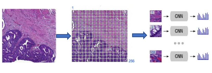
Figure 19: The VGG-16 network produces a high-dimensional feature vector for each individual tile from an input image. This figure corresponds to Fig.1 in Bychkov-2018-DLTA .

Deep Learning Features of the ResNet Series

ResNet is another widely used CNN structure. The full name of ResNet is Residual Network and the proponent is Balduzzi D. ResNet has pushed deep learning to a new level, reducing the error rate to a level lower than that of humans for the first time. The residual module in ResNet makes the network deeper, but with lower complexity. It also makes the network easier to optimize and solves the problem of vanishing gradient He-2016-DRLI . The bottlen neck layer in ResNet uses 1$\texttimes$1 networks, which expands the dimension of the featuremap and greatly reduces the amount of calculation He-2016-IMDR . Among the papers we reviewed, the papers that use ResNet to extract deep learning features include Korbar-2017-DLCC ; Korbar-2017-LUHD ; Kwok-2018-MCBC ; Campanella-2018-TSDM ; Jiang-2018-TMDD ; Shou-2018-WSIC ; Bertram-2019-LSDM ; Xu-2019-MTPW .

Deep Learning Features of the U-net Series

The full name of U-net is Unity Networking. it is a network architecture established to solve the problem of medical image segmentation. This structure is based on FCN (Fully Convolutional Neural Network). It adds an upsampling stage and adds many feature channels, allowing more original image texture information in high-resolution layers, using valid for convolution throughout, ensuring that the results obtained are based on no missing context features Ronneberger-2015-UCNB . In the paper we summarized, the use of U-net for deep learning feature extraction have Bandi-2017-CDMT ; Seth-2019-ALBD ; Seth-2019-ASDW ; Feng-2020-DLMA .

Other Deep Learning Feature

There are other improved structures based on CNN, such as GoogLeNet Wang-2016-DLIM . The Google Academic team carefully prepares GoogLeNet to participate in the ILSVRC 2014 competition. The main idea is to approximate the optimal sparse structure by building a dense block structure to improve performance without increasing the amount of calculation. The initial version of GoogLeNet appeared in Szegedy-2015-GDC .

There are also other improved structures based on Recurrent Neural Networks (RNN) Maksoud-2019-CCOR and LSTM  Ren-2018-DPCP , which are used to extract deep learning features. RNN appeared in the 1980s, and its prototype has seen in the Hopfield neural network model proposed by American physicists in 1982 Hopfield-1982-NNPS . RNN has a strong processing ability for variable length sequence data. Therefore, it is very effective for data with time-series characteristics and can mine time series information and language information in the data. The Long Short-Term Memory (LSTM) model appeared because of the drawbacks of RNN, and LSTM can solve the problem of gradient disappearance in RNN Hochreiter-1997-LSTM .

3.3 Summary

It can be seen from the content we reviewed above, in the traditional feature extraction, color feature, texture feature, and shape feature are the three most commonly used features. The texture feature is the most used. In the papers we summarized, from 2004 to 2019, a total of 51 papers used texture features. The second is color features, which are generally based on the three color spaces of RGB, HSV, and LAB. Among them, the RGB color space is the most commonly used. The least applied is the shape feature. For more details and analysis in this regard, see the detailed introduction in the following chapters.

Over times, the level of science and technology has also continuously improved. As can be seen from the papers we summarized, since 2016, deep learning features have been gradually applied to this day. The specific deep learning network architecture will be introduced in a separate method analysis later. Table. LABEL:CDFE is a summary of the CAD methods used for feature extraction in WSI.

Table 4: Summary of the CAD methods used for feature extraction in WSI (Traditional (T)).

Feature Type	Method	Reference	Year	Team	Details
T	Color	Kong-2009-CAEN	2009	J Kong, O Sertel	Combined Color and entropy information extracted from RGB and LAB image channels
T	Color	Roullier-2010-GMRS	2010	V. Roullier	RGB feature vector
T	Color	Samsi-2012-ECFA	2012	Siddharth Samsi	Hue channel for HSV color space conversion
T	Color	Kothari-2012-BIMP	2012	Sonal Kothari	RGB, CIELAB, HSV, mean and standard deviation in each channel in three spaces
T	Color	Akakin-2012-CBMI	2012	Hatice Cinar Akakin	Nuclear RGB features
T	Color	Collins-2013-AMAU	2013	Brian T. Collins	color information
T	Color	Nayak-2013-CTHS	2013	Nandita Nayak	The average, standard deviation, minimum and maximum values of each color channel in the RGB space
T	Color	Veta-2013-DMFB	2013	M. Veta	$\backslash$
T	Color	Kothari-2013-ETFA	2013	Kothari S	PVS for each R, G, B and H, S, V channel
T	Color	Homeyer-2013-PQNH	2013	André Homeyer	Variance of RGB, $/mu$ hue of HIS
T	Color	Hiary-2013-SLWS	2013	Hazem Hiary	RGB color and color saturation and value in HSV space
T	Color	Bautista-2014-CSWS	2014	Pinky A. Bautista	RGB color and color saturation and value in HSV space RGB
T	Color	Mercan-2014-LDRR	2014	Ezgi Mercan	Lab space color histogram
T	Color	Yeh-2014-MSDP	2014	Fang‑Cheng Yeh	RGB color channels
T	Color	Litjens-2015-ADPC	2015	Litjens, G	RGB histogram features
T	Color	Weingant-2015-EPTC	2015	Michaela Weingant	color channel histogram
T	Color	Li-2015-FRID	2015	Ruoyu Li	Histogram of the three-channel HSD color model
T	Color	Mercan-2016-LDRR	2016	Mercan E	LAB histograms for color
T	Color	Barker-2016-ACBT	2016	Barker J	$\backslash$
T	Color	Mercan-2016-MIML	2016	Mercan, C	LAB histograms for Color
T	Color	Brieu-2016-SSMS	2016	Brieu N, Pauly O	$\backslash$
T	Color	Mercan-2017-MIML	2017	Caner Mercan	color histogram of each channel in CIE-LAB space
T	Color	Cruz-2018-HTAS	2018	Angel Cruz-Roa	color Histograms 8 × 3 8-bin histogram for each RGB channel
T	Color	Morkunas-2018-MLBC	2018	Morkūnas M	The average and standard deviation of the pixel values of each color channel and its RGB superpixels.
T	Texture	Diamond-2004-UMCT	2004	JamesDiamondPhDa	$\backslash$
T	Texture	Petushi-2006-LSCH	2006	Sokol Petushi	9 texture parameters: DNM1, DNM2, DNM3, DNM1-2, DNM1-3, DNM2-3, DNM1-2-3, DT, DN
T	Texture	Sertel-2008-CAPN	2008	Olcay Sertel	LBP features,Haralick features
T	Texture	Sertel-2009-CCCS	2009	O Sertel	$\backslash$
T	Texture	Kong-2009-CAEN	2009	J Kong, O Sertel	Four textural Haralick features
T	Texture	Sertel-2009-CPNW	2009	O Sertel, J Kong	LBP features
T	Texture	Roullier-2010-MEBC	2010	Vincent Roullier	LBP histogram
T	Texture	Difranco-2011-ESWS	2011	Matthew D. DiFranco	Feature maps(the mean and standard from HS), Co-occurrence texture features
T	Texture	Kong-2011-IMAG	2011	Jun Kong	Texture and gradient features
T	Texture	Roullier-2011-MRGA	2011	Vincent Roullier	LBP
T	Texture	Grunkin-2011-PCIA	2011	Michael Grunkin	$\backslash$
T	Texture	Nguyen-2011-PCDF	2011	Kien Nguyen	Gabor filter features
T	Texture	Doyle-2010-BBMC	2012	Scott Doyle	Co-occurrence Features
T	Texture	Akakin-2012-CBMI	2012	Hatice Cinar Akakin	Mean, standard deviation, contrast, correlation, energy, entropy and uniformity
T	Texture	Sharma-2012-DSHI	2012	Harshita Sharma	Texton-based texture
T	Texture	Nayak-2013-CTHS	2013	Nandita Nayak	$\backslash$
T	Texture	Jiao-2013-CCDU	2013	Liping Jiao	Combine mean, variance and other 17 features which are extracted by GLCM method
T	Texture	Veta-2013-DMFB	2013	M. Veta	$\backslash$
T	Texture	Kothari-2013-ETFA	2013	Kothari S	$\backslash$
T	Texture	Kong-2013-MBMA	2013	Jun Kong	$\backslash$
T	Texture	Homeyer-2013-PQNH	2013	André Homeyer	$\backslash$
T	Texture	Hiary-2013-SLWS	2013	Hiary H, Alomari R S	$\backslash$
T	Texture	Apou-2014-FSTC	2014	Apou G, Naegel B	$\backslash$
T	Texture	Mercan-2016-LDRR	2014	Ezgi Mercan	LBP
T	Texture	Bejnordi-2015-MSSC	2015	Bejnordi, B. E	LBP
T	Texture	Sharma-2015-ABND	2015	Harshita Sharma	GLCM Features
T	Texture	Swiderska-2015-CMSA	2015	Zaneta Swiderska	$\backslash$
T	Texture	Weingant-2015-EPTC	2015	Michaela Weingant	GLCM features
T	Texture	Li-2015-FRID	2015	Ruoyu Li	$\backslash$
T	Texture	Zhang-2015-FGHI	2015	Xiaofan Zhang	$\backslash$
T	Texture	Cooper-2015-NGPA	2015	Lee AD Cooper	$\backslash$
T	Texture	Apou-2015-SWSI	2015	Gregory Apou	$\backslash$
T	Texture	Peikari-2015-TDRR	2015	Peikari M	$\backslash$
T	Texture	Mercan-2016-LDRR	2016	Mercan E	LBP
T	Texture	Barker-2016-ACBT	2016	Barker J	$\backslash$
T	Texture	Bejnordi-2016-ADDW	2016	Bejnordi B E	$\backslash$
T	Texture	Zhao-2016-AGEW	2016	Zhao Y	GLCM
T	Texture	Harder-2016-CFCG	2016	Harder N	Co-occurrence Feature
T	Texture	Shirinifard-2016-DPAU	2016	Shirinifard A	$\backslash$
T	Texture	Gadermayr-2016-DACC	2016	Gadermayr M	HOG,LBP,FV
T	Texture	Leo-2016-ESHF	2016	Leo P, Lee G	Haralick features
T	Texture	Mercan-2016-MIML	2016	Mercan, C	LBP
T	Texture	Brieu-2016-SSMS	2016	Brieu N, Pauly O	$\backslash$
T	Texture	Saltz-2017-CSSG	2017	Saltz, J	$\backslash$
T	Texture	Babaie-2017-CRDP	2017	Babaie M	LBP
T	Texture	Hu-2017-DLBC	2017	Hu J X	Haralick texture
T	Texture	Bejnordi-2017-DADL	2017	Bejnordi B E	SIFT,LBP,GLCM
T	Texture	Valkonen-2017-MDWS	2017	Valkonen M	VLFeat implementation of MSER and SIFT
T	Texture	Mirschl-2018-DLCI	2018	Jeffrey J. Nirschl	$\backslash$
T	Texture	Xu-2018-AACM	2018	Hongming Xu	$\backslash$
T	Texture	Yoshida-2018-AHCWG	2018	Hiroshi Yoshida	$\backslash$
T	Texture	Han-2018-ACDL	2018	W. Han	$\backslash$
T	Texture	Morkunas-2018-MLBC	2018	Morkūnas M	$\backslash$
T	Texture	Mercan-2017-MIML	2018	Caner Mercan	$\backslash$
T	Texture	Simon-2018-MRLF	2018	Olivier Simon	LBP,mrcLBP feature
T	Texture	Klimov-2019-WSIB	2019	S Klimov	$\backslash$
T	Shape	Diamond-2004-UMCT	2004	JamesDiamondPhDa	$\backslash$
T	Shape	Kong-2011-IMAG	2011	Jun Kong	$\backslash$
T	Shape	Grunkin-2011-PCIA	2011	Michael Grunkin	$\backslash$
T	Shape	Lu-2012-ASAE	2012	Cheng Lu	$\backslash$
T	Shape	Kothari-2012-BIMP	2012	Sonal Kothari	$\backslash$
T	Shape	Veta-2012-PVAE	2012	Mitko Veta	$\backslash$
T	Shape	Lopez-2013-ABDM	2013	Lopez X M	Multiple sharpness features
T	Shape	Collins-2013-AMAU	2013	Brian T. Collins	$\backslash$
T	Shape	Veta-2013-DMFB	2013	M. Veta	$\backslash$
T	Shape	Kothari-2013-ETFA	2013	Kothari S	$\backslash$
T	Shape	Kong-2013-MBMA	2013	Jun Kong	$\backslash$
T	Shape	Cooper-2015-NGPA	2015	Lee AD Cooper	$\backslash$
T	Shape	Barker-2016-ACBT	2016	Barker J	$\backslash$
T	Shape	Wang-2016-DLIM	2016	Dayong Wang Aditya Khosla	$\backslash$
T	Shape	Saltz-2017-CSSG	2017	Saltz, J	$\backslash$
T	Shape	Xu-2018-AACM	2018	Hongming Xu	$\backslash$
DL	CNN	Puerto-2016-DPAW	2016	Puerto M	$\backslash$
DL	CNN	Sharma-2016-DCNN	2016	Sharma H	$\backslash$
DL	CNN	Wang-2016-DLIM	2016	Dayong Wang Aditya Khosla	GoogLeNet
DL	CNN	Geccer-2016-DCBC	2016	Geçer B	$\backslash$
DL	CNN	Sirinukunwattana-2016-LSDL	2016	Sirinukunwattana K	NEP coupled with CNN
DL	CNN	Hou-2016-PCNN	2016	Hou L	$\backslash$
DL	CNN	Sheikhzadeh-2016-ALMB	2016	Sheikhzadeh F	CNN,FCN
DL	CNN	Cruz-2017-ARIB	2017	Cruz-Roa A	$\backslash$
DL	CNN	Wollmann-2017-AGBC	2017	Wollmann T	DNN
DL	CNN	Araujo-2017-CBCH	2017	Araújo T	Patch-wise trained CNN
DL	CNN	Bandi-2017-CDMT	2017	Bándi P	FCN,U-net
DL	CNN	Bejnordi-2017-CASC	2017	Bejnordi B E	Context-aware stacked CNN
DL	CNN	Sharma-2017-DCNN	2017	Sharma H	Selected self-designed CNN architecture
DL	CNN	Korbar-2017-DLCC	2017	Korbar B	A modified version of a ResNet architecture
DL	CNN	Jimenez-2017-DMCR	2017	Jimenez-del-Toro O	$\backslash$
DL	CNN	Xu-2017-LSTH	2017	Xu Y	$\backslash$
DL	CNN	Korbar-2017-LUHD	2017	Korbar B	ResNet
DL	CNN	Ghosh-2017-SLCA	2017	Ghosh A	Deep convolutional network
DL	CNN	Das-2017-CHWS	2017	Das K, Karri S P K	self-designed CNN
DL	CNN	Cui-2018-DLAO	2018	Cui Y	FCN
DL	CNN	Zanjani-2018-CDHW	2018	Farhad Ghazvinian Zanjani	Apply CRFs over latent spaces of a trained deep CNN
DL	CNN	Courtiol-2018-CDLH	2018	Courtiol P	ResNet
DL	CNN	Kumar-2018-DBFR	2018	Meghana Dinesh Kumar	VGG,AlexNet
DL	CNN	Bychkov-2018-DLTA	2018	Dmitrii Bychkov	VGG
DL	CNN	Gecer-2018-DCCW	2018	Baris Gecer	FCN
DL	RNN	Ren-2018-DPCP	2018	Jian Ren	LSTM
DL	CNN	Tellez-2018-GWSI	2018	David Tellez	Self-designed CNN
DL	CNN	Sirinukunwattana-2018-IWSS	2018	K Sirinukunwattana	Self-designed CNN
DL	CNN	Kwok-2018-MCBC	2018	Scotty Kwok	Inception-Resnet-v2
DL	CNN	Das-2018-MILD	2018	Kausik Das	A MIL framework for CNN
DL	CNN	Lin-2018-SFDS	2018	Huangjing Lin	FCN
DL	CNN	Campanella-2018-TSDM	2018	Campanella G	VGG and ResNet
DL	CNN	Jiang-2018-TMDD	2018	Jiang S	ResNet
DL	CNN	Wang-2018-WSLW	2018	X Wang	VGG
DL	CNN	Shou-2018-WSIC	2018	Junni Shou	DenseNet
DL	CNN	Tellez-2018-WSMD	2018	David Tellez	$\backslash$
DL	CNN	Seth-2019-ALBD	2019	Nikhil Seth	U-Net
DL	CNN	Bertram-2019-LSDM	2019	Christof A. Bertram	ResNet
DL	CNN	Li-2019-AMRM	2019	Jiayun Li	VGG
DL	CNN	Liu-2019-AIBC	2019	Liu Y	Inception
DL	CNN	Campanella-2019-CGCP	2019	Gabriele Campanella	A MIL framework for CNN
DL	CNN	Yue-2019-CCOP	2019	Xingzhi Yue	VGG
DL	RNN	Maksoud-2019-CCOR	2019	Sam Maksoud	LSTM
DL	CNN	Bilaloglu-2019-EPCW	2019	S Bilaloglu	PathCNN(Self-designed)
DL	CNN	Lin-2019-FSFD	2019	Huangjing Lin	VGG
DL	CNN	Yu-2019-LSGC	2019	H Yu, X Zhang	DNN
DL	CNN	Sanghvi-2019-PAIA	2019	Adit B. Sanghvi, MISM	$\backslash$
DL	$\backslash$	Wang-2019-RRMI	2019	Shujun Wang	RMDL
DL	CNN	Kohlberger-2019-WSIF	2019	Kohlberger T	ConvFocus(based CNN)
DL	CNN	Seth-2019-ASDW	2019	Seth N, Akbar S	U-net
DL	CNN	Xu-2019-MTPW	2019	Xu J	ResNet and DenseNet
DL	CNN	Feng-2020-DLMA	2020	Feng Y, Hafiane A	U-net
DL	CNN	Chen-2020-ITWS	2020	Chen P, Shi X	DeepCIN(CNN,BLSTM)
DL	CNN	Sornapudi-2020-CWSH	2020	Sornapudi S, Addanki R	$\backslash$
DL	CNN	Pantanowitz-2020-AIAP	2020	Pantanowitz L	Self-designed CNN

Table 4: Continue: Summary of the CAD methods used for feature extraction in WSI.

4 Segmentation Methods

In recent years, with the increasing size and quantity of medical images, computers must facilitate processing and analysis. In particular, computer algorithms for delineating anatomical structures and other areas of interest are becoming increasingly important in assisting and automating specific histopathological tasks. These algorithms are called image segmentation algorithms Pham-2000-CMMI .

Image segmentation refers to the process of dividing a digital image into multiple segments, namely a set of pixels. The pixels in a region are similar according to some homogeneity criteria (such as color, intensity, or texture), to locate and identify objects and boundaries in the image  Gonzalez-2007-IP . The practical applications of image segmentation include: filtering noise images, medical applications (locating tumors and other pathologies, measuring tissue volume, computer-guided surgery, diagnosis, treatment planning, anatomical structure research)  Patil-2013-MISR , locating objects in satellite images (roads, forests, etc.), facial recognition, fingerprint recognition, etc. The selection of segmentation techniques and the level of segmentation depends on the specific type of image and the characteristics of the problem being considered Dass-2012-IST1 .

In the process of medical image segmentation, the details required in the segmentation process largely depend on the clinical application of the problems Masood-2015-SMIS  Zuva-2011-ISAT . The purpose of segmentation is to improve the visualization process to deal with the detection process more effectively. Medical image segmentation is faced with many problems because the quality of the segmentation process is affected Shrimali-2009-CTSM . When there is noise in the image, there will be uncertainty, which makes it difficult to classify the image Birkfellner-2016-AMIP . The reason is that the intensity value of the pixel has been modified due to noise in the image. Such a change in pixel intensity value will disturb the uniformity of the image intensity range Al-2010-CSRN . Therefore, to deal with this uncertainty, image segmentation plays a crucial role in medical diagnostic systems He-2013-MIS .

As a crucial step in CAD pathologists, segmentation techniques have flourished in recent years. As shown in Fig. 2, from 2010 to 2020, the number of papers using segmentation WSI technology to assist doctors in diagnosis has increased from 2 to 28. According to the papers we have reviewed, segmentation is divided into five different techniques including thresholding-based, region-based, graph-based, clustering-based, deep learning, and other image segmentation methods. Its composition and structure diagram are shown in Figure. 20.

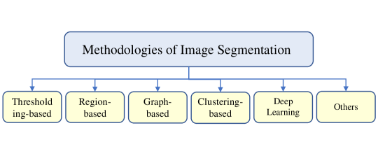
Figure 20: The composition of the segmentation method in WSI.

4.1 Thresholding based Segmentation Method

Threshold segmentation is a classic method in image segmentation. It uses the difference in grayscale between the target and the background to be extracted in the image, and divides the pixel level into several categories by setting a threshold to achieve the separation of the target and the background Fu-1981-SIS ; Haralick-1985-IST . The threshold segmentation method is simple to calculate, and can always use closed and connected boundaries to define non-overlapping regions. Images with a strong contrast between the target and the background can provide better segmentation effect Sahoo-1988-STT .

Among them, the selection of the optimal threshold is a significant issue. Commonly used threshold selection methods are: manual experience selection method, histogram method Rosenfeld-1983-HCAA , maximum between-class variance method (OTSU) Ohtsu-1978-DLST , adaptive threshold method. Because the threshold segmentation method is simple to implement, the amount of calculation is small, and the performance is relatively stable, it has become the most in image segmentation. As the basic and most widely used segmentation technology, it has been used in many fields. Among the reviewed papers, five are based on threshold based segmentation Kong-2011-IMAG ; Lu-2012-ASAE ; Shu-2013-SOCN ; Vo-2016-CWSI ; Arunachalam-2017-CAIS .

In Kong-2011-IMAG , an image analysis tool for segmentation and characterization of cell nuclei is developed. The microscopic images of glioblastoma from the TCGA project are used. To reliably identify cell nuclei, a fast hybrid gray-scale reconstruction algorithm is applied to the image to normalize the background area degraded by artifacts produced by tissue preparation and scanning Vincent-1993-MGRI . This operation separates the foreground from the normalized background and allows simple threshold processing to identify the nucleus.

In Lu-2012-ASAE , a computer-aided technique is proposed for segmentation and analysis of the whole slide skin histopathological images. Before using the segmentation technique, determine the single-color channel that provides good discrimination information between the epidermis and dermis regions. Then multi-resolution image analysis is used in the proposed segmentation technique. First, a low-resolution image of the WSI is generated. Then, the global threshold method and shape analysis to segment low-resolution images are used. Based on the segmented skin area, the layout of the skin is determined, and a high-resolution image block of the skin is generated for further manual or automatic analysis. Experiments on 16 different whole slide skin images show that the technology has high performance, $92\%$ sensitivity, $93\%$ accuracy, and $97\%$ specificity are achieved.

In Shu-2013-SOCN , a new method is proposed to segment severely aggregated overlapping cores. The proposed method first involves applying a combination of global and local thresholds to extract foreground regions.

In Vo-2016-CWSI and Vo-2019-MCMH , a highly scalable and cost-effective image analysis framework based on MapReduce is proposed, and a cloud-based implementation is provided. The framework adopts a grid-based overlap segmentation scheme and provides parallelization of image segmentation based on MapReduce. In the segmentation step, a threshold method is applied to segment the nucleus.

In Arunachalam-2017-CAIS , the segmentation of tumor and non-tumor areas on the WSIs datasets of osteosarcoma histopathology. The method in this article combines pixel-based and object-based methods, using tumor attributes, such as nucleus clusters, density, and circularity, and using multi-threshold Otsu segmentation technology to further classify tumor regions as live and inactive. The pan-fill algorithm clusters similar pixels into cell objects and calculates the cluster data to analyze the studied area further. The final experimental results show that for all the sampled datasets used, the accuracy of the method in question in identifying live tumors and coagulative necrosis is $100\%$, while the accuracy of fibrosis and acellular/low cell tumors is about $90\%$. The WSI effect after multi-threshold Otsu segmentation is shown in Figure. 21.

Figure 21: Otsu output showing more blue color. This figure corresponds to Fig.3 in Arunachalam-2017-CAIS .

4.2 Region-based Segmentation Method

Region-based segmentation is a kind of segmentation techniques based on directly finding the region. In fact, similar to the boundary-based image segmentation technology, it uses the similarity of the object’s gray distribution and background. Generally, region-based image segmentation methods contain two categories: watershed segmentation and region growing.

Watershed Segmentation

The watershed algorithm draws on the theory of morphology and is a region-based image segmentation algorithm. In this method, an image is regarded as a topographic map, and the gray value corresponds to the height of the terrain. High gray values correspond to mountains, and low gray values correspond to valleys. If rain falls on the surface, the low-lying area is a basin, and the ridge between the basins is called a watershed. Watershed is equivalent to an adaptive multi-threshold segmentation algorithm Vincent-1991-WDSE .

In Kong-2011-IMAG , overlapping nuclei are separated using the watershed method. In Veta-2012-PVAE , an automatic cell nucleus segmentation algorithm is used to extract size-related morphometric features of cell nuclei and analyze their prognostic value in male breast cancer. The segmentation process consists of four main steps: preprocessing, watershed segmentation controlled by multi-scale markers, post-processing, and merging of multi-scale results. The overall process of this automatic segmentation method is shown in the Figure. 22. In Veta-2013-ANSH , the same automatic segmentation method as in  Veta-2012-PVAE is used in H&E stained breast cancer histopathology images.

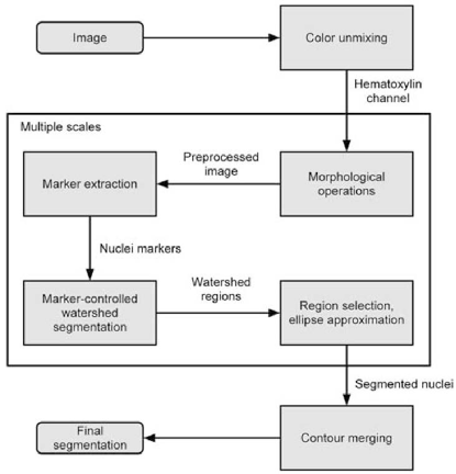
Figure 22: Overview of the automatic nuclei segmentation method. This figure corresponds to Fig.1 in Veta-2012-PVAE .

In  Shu-2013-SOCN , to segment the overlapping nuclei gathered in the foreground region, seed markers are obtained using morphological filtering and intensity-based region growth. Then the seed watershed and separate the aggregated nuclei are applied. Finally, a post-processing step of identifying positive nuclear pixels is added to eliminate false pixels. Some segmentation results are shown in Fig. 23. In Vo-2016-CWSI and Vo-2019-MCMH , watershed technology is used to separate overlapping nuclei in objects is used.

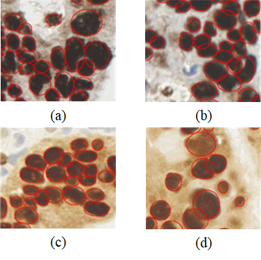
Figure 23: Some segmentation results. This figure corresponds to Fig.7 in Shu-2013-SOCN .

Region Growing

Region growing is an image segmentation method of serial region segmentation. Region growth refers to starting from a certain pixel and gradually adding neighboring pixels according to specific criteria. When certain conditions are met, the regional growth is terminated, that is, The region’s growth depends on the selection of the initial point (seed point), growth criteria, and termination conditions Hojjatoleslami-1998-RGNA .

The region growing is relatively a common method. It can achieve the best performance when there is no prior knowledge available, and it can be used to segment more complex images. However, the regional growth method is iterative, and space and time costs are relatively high  Adams-1994-SRG . Among the WSI-based segmentation tasks we have summarized, there is one paper related to region growth Shu-2013-SOCN .

4.3 Graph-based Segmentation Method

Graph-based segmentation is a classic image segmentation algorithm. The algorithm is a greedy clustering algorithm based on the graph. Its advantages include simple implementation and faster speed Felzenszwalb-2004-EGIS . Many popular algorithms are based on this method Van-2011-SSSO .

Graph-based segmentation first expresses image as a graph in graph theory, so that, each point in a pixel is regarded as a vertex $v_{i}\in V$, and each pixel and 8 adjacent pixels (eight neighborhoods) form a graph edge $e_{i}\in E$, so a graph $G=(V,E)$ is constructed. The weight of each side of the graph is the relationship between the pixel and the neighboring pixels, which expresses the similarity between the neighboring pixels. Treat each node (pixel) as a single area, and then merge it according to the parameters of the area and the internal difference to get the final segmentation West-1996-IGH .

Because WSIs are usually very large, they are stored as pyramids of tiled images, so that they can be processed in a hierarchical manner, that is, low-resolution to determine the area of interest, high-resolution image classification, top-down segmentation. Among the papers we reviewed, there are three papers that combine graph-based segmentation methods with multi-resolution Roullier-2011-MRGA ; Roullier-2010-GMRS ; Roullier-2010-MEBC .

In  Roullier-2010-GMRS , Roullier-2010-MEBC and Roullier-2011-MRGA , the mitosis in WSI of breast tissue is extracted. The image is simplified by discrete regularization, and clustering is performed by unsupervised 2-mean clustering. Clustering is performed in a specific area divided at the previous resolution. The obtained clusters are expanded with finer resolution levels through pixel duplication and refined in specific areas. At the last resolution level, the mitotic figure is extracted. The segmentation result of mitosis in Roullier-2010-GMRS is shown in the Figure. 24.

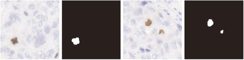
Figure 24: The composition of the segmentation method in WSI. This figure corresponds to Fig.3 in Roullier-2010-GMRS

4.4 Clustering-based Segmentation Method

Clustering is based on the relationship between each pixel and neighboring pixels. If a pixel is similar in color, texture, or gray to its neighboring pixels, then they will be merged into the same class.

$k$-means algorithm is more commonly used in clustering algorithms. The cluster center point is obtained by calculating the average of all pixels in each cluster in the sample. The basic working principle of the $k$-means algorithm is to receive the parameter $k$ input by the user, divide the given $n$ data sample points into $k$ groups on average, take the input $k$ points as the cluster centers to be converged, and calculate the other clusters. The Euclidean distance from the sampling point to the $k$ convergence centers. And compare the distance between all sampling points and the convergence center point. The classification is made by comparing the minimum form of Euclidean distance. Then after repeated iterations, the mean value of $k$ clusters is successively obtained. Until the performance criterion function, clustering is the best, the overall error is the smallest, and the best clustering effect is obtained Macqueen-1967-SMCA .

Among the papers we reviewed, the papers on $k$-means clustering and segmentation are Hiary-2013-SLWS and Arunachalam-2017-CAIS . In Hiary-2013-SLWS , the author uses $k$-means unsupervised learning for WSI segmentation, which produces a highly robust correctness result equivalent to supervised learning, which is $95.5\%$ accuracy. In Arunachalam-2017-CAIS , the $k$-means clustering technique with color normalization is used for tumor separation.

4.5 Deep Learning based Segmentation

Among the papers we reviewed, 10 papers used deep learning methods for WSI segmentation Bandi-2017-CDMT ; Xu-2017-LSTH ; Dong-2018-RANT ; Cui-2018-DLAO ; Sirinukunwattana-2018-IWSS ; Mehta-2018-LSBB ; Vo-2019-MCMH ; Seth-2019-ALBD ; Seth-2019-ASDW ; Feng-2020-DLMA .

In Bandi-2017-CDMT , two different CNN structures, FCN and U-net, are used to segment and accurately identify tissue slices. Here, the two methods are compared with the traditional foreground extraction (FESI) algorithm based on structural information. These three methods are applied to 54 WSIs, and the average value of the Yakoka index and the standard deviation of the Yakoka index are used for evaluation. The final U-net result is the best (Jaccard index is 0.937). The qualitative effects of different algorithms are shown in Figure. 25.

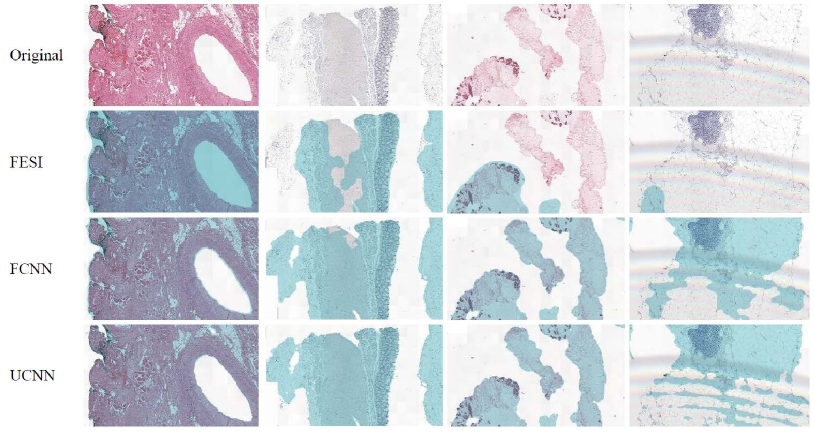
Figure 25: Qualitative results for the different algorithms. This figure corresponds to Fig.2 in Bandi-2017-CDMT

In Xu-2017-LSTH , CNN-based ImageNet is used to extract features and convert them into histopathological images. And Support Vector Machine (SVM) is used to define segmentation as a classification problem. This method is applied to the digital pathology and colon cancer dataset of the MICCAI 2014 Challenge, and finally won the first place with $84\%$ test data accuracy.

In Dong-2018-RANT , a simple and effective framework called Reinforced Auto-Zoom Net (RAZN) is proposed, which considers the accurate and fast prediction of breast cancer segmentation. RAZN learns a strategy network to decide whether to zoom on a given area of interest. Because the amplification action is selective, RAZN is robust to unbalanced and noisy ground truth labels and effectively reduces overfitting. Finally, the method is evaluated on the public breast cancer dataset. It can be seen from the experimental results that RAZN is superior to single-scale and multi-scale baseline methods, and obtains better accuracy with lower inference cost.

In Cui-2018-DLAO , an automatic end-to-end deep neural network algorithm is proposed to segment the single core. The kernel-boundary model is introduced to predict the kernel and its boundary simultaneously using FCN. Given the color normalized image, the model directly outputs the estimated kernel map and boundary map. After post-processing, the final segmented core is produced. A method for extracting and assembling overlapping blocks is designed to seamlessly predict the cores in a large WSI. The final result proves the effectiveness of the data expansion method for cell nucleus segmentation tasks. The experiment shows that this method is superior to the prior art method and it is possible to accurately segment WSI within an acceptable time.

In Sirinukunwattana-2018-IWSS , different architectures are systematically compared to evaluate how the inclusion of multi-scale information affects segmentation performance. The architectures are shown in Figure. 26. It uses a public breast cancer dataset and a locally collected prostate cancer dataset. The result shows that the visual environment and scale play a vital role in the classification of histological images.

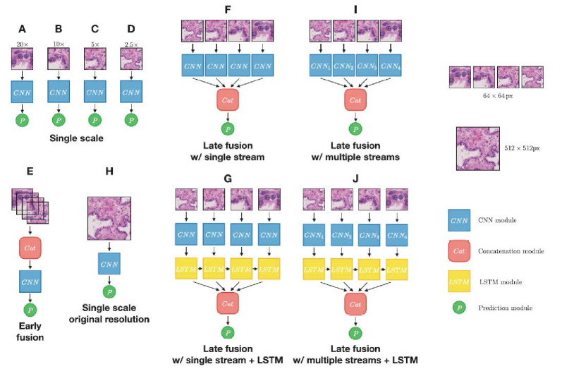
Figure 26: Used architectures. This figure corresponds to Fig.2 in Sirinukunwattana-2018-IWSS

In Mehta-2018-LSBB , a new encoder-decoder architecture is proposed to solve the semantic segmentation problem of breast biopsy WSI. The designed new architecture contains four new functions: (1) Input Perceptual Coding Block (IA-RCU), which enhances the input inside the encoder to compensate for the loss of information due to down-sampling operations, (2) densely connected decoding network and (3) additional sparsely connected decoding network to effectively combine the multi-level features aggregated by the encoder, and (4) a multi-resolution network for context-aware learning, which uses densely connected fusion blocks to combine different resolutions rate output. The architecture is shown in Figure. 27. The result after segmentation is shown in Figure. 28.

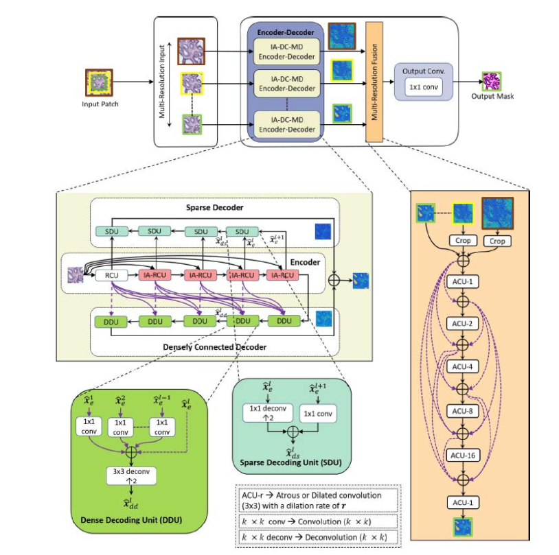
Figure 27: Multi-resolution encoder-decoder network structure diagram. This figure corresponds to Fig.4 in Mehta-2018-LSBB .

Figure 28: Segmentation result. The first line describes aggressive cases, while the second line describes benign cases. This figure corresponds to Fig.9 in Mehta-2018-LSBB .

In Seth-2019-ALBD and Seth-2019-ASDW , several U-net architectures-DCNN designed to output probability maps are trained to segment ductal carcinoma in-situ (DCIS) WSI in wireless sensor networks and verified the minimum required to achieve excellent accuracy at the slide level good patch vision. U-net is trained five times to achieve the best test results (DSC = 0.771, F1 = 0.601), which means that U-net benefits from seeing wider contextual information.

In Feng-2020-DLMA , a multi-scale image processing method is proposed to solve the segmentation problem of liver cancer in histopathological images. These eight networks are compared, and then the network most suitable for liver cancer segmentation is selected. Through a comprehensive comparison of performance, U-net is selected. The local color normalization method of pathological images is used to solve the influence of the background, and then a seven-layer Gaussian pyramid representation is established for each WSI to obtain a multi-scale image set. The trained U-net is fine-tuned at each level to obtain an independent model. Then, shift cropping and weighted overlap are used in the prediction process to solve block continuity. Finally, the predicted image is mapped back to the original size, and a voting mechanism is proposed to combine the multi-scale predicted images. The experimental data are the verification images of the 2019 MICCAI PAIP Challenge. The evaluation results show that this algorithm is better than other algorithms.

4.6 Other Segmentation Methods

In Bergmeir-2012-SCCN , a new algorithm for segmenting cell nuclei is used. Before determining the precise shape of the cell nucleus by the elastic segmentation algorithm, the proposed algorithm uses a voting scheme and prior knowledge to locate the cell nucleus. After removing noise through the mean shift and median filtering, the Canny edge detection algorithm is used to extract edges. Since the nucleus is observed to be surrounded by cytoplasm, its shape is roughly elliptical, and the edges adjacent to the background are removed. The random hough transform of the ellipse finds the candidate kernel, and then processes it through the level set algorithm. The algorithm is tested and compared with other algorithms in a database containing 207 images obtained from two different microscope slides, and the results passed the positive predictive value (PPV) and TPR. The high value of, is displayed, resulting in a high measurement value of $96.15\%$.

In Apou-2014-FSTC , a fast segmentation method based on WSI is proposed. Due to the large size of the WSI, a set of horizontal and vertical optimal paths that follow the high gradient of the image are used to segment the image so that the relevant segmentation of the image is provided in an effective manner. Then other subsequent steps are executed. The schematic diagram of the segmentation process is shown in Figure. 29.

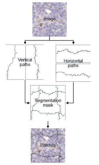
Figure 29: Path computation in horizontal and vertical strips, leading to an image partition. This figure corresponds to Fig.4 in Apou-2014-FSTC

In Zhang-2015-FGHI , a robust segmentation method is developed to accurately delineate ROI (eg, cells) using hierarchical voting and repelling active contours. Its segmentation is based on active contours with repelling terms Cohen-1991-OACM . The exclusion term is used to prevent the contour lines from intersecting and merging. Based on the detection result, the circle is associated with each detected cell as the initial contour. The final segmentation result is shown in Figure. 30.

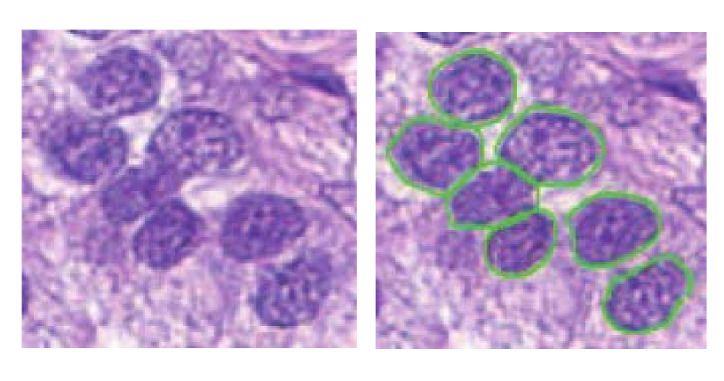
Figure 30: Segmentation results of different methods on a randomly picked patch. From left to right: original image and ours. This figure corresponds to Fig.3 in Zhang-2015-FGHI

.

In Li-2015-FRID , a new ROI search and segmentation algorithm based on superpixels is proposed. First, the initial recognition of the ROI is obtained by gathering superpixels at low magnification. Then, by marking the corresponding pixels, the superpixels are mapped to the higher magnification image. This process is repeated several times until the segmentation is stable. This method is different from the previous classic segmentation methods based on superpixels Achanta-2012-SSCS ; Yamaguchi-2014-EJSO . This algorithm provides image segmentation with topology preservation.

In Brieu-2016-SSMS , threshold processing is performed on the foreground posterior image to detect the foreground area, and spot detection algorithms such as MSER and Gaussian difference are used further to identify the brightness of the image. According to the classification function combining suitable candidate parameters are selected. The remaining area is further divided by calculating the minimum path of the posterior mapping between the concave points and checking the goodness of fit of the candidate area in turn. The schematic diagram after segmentation is shown in Figure. 31.

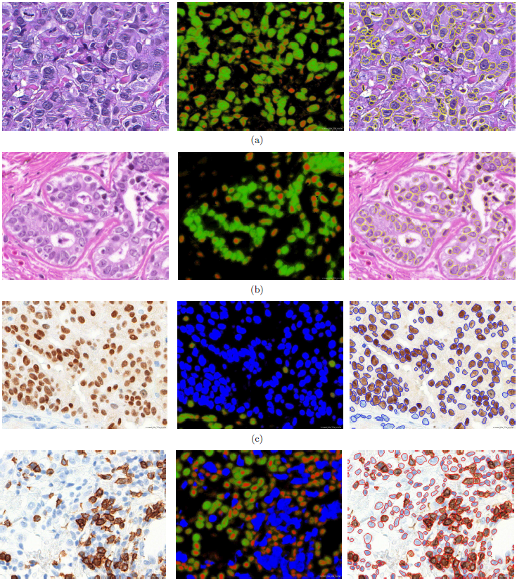
Figure 31: The schematic diagram after segmentation is shown in the figure. Left: H&E (a)-(b), IHC-nuclei (c), and CD8 (d) regions; Center: posterior maps for marked nuclei and cells (blue channel if applicable), for homogeneous nuclei (red channel) and for textured nuclei (green channel); Right: outline of the segmentation result. This figure corresponds to Fig.3 in Brieu-2016-SSMS .

4.7 Summary

As can be seen from the content we reviewed above, machine learning is used in combination with WSI technology to assist diagnosis. In the field of image segmentation, used methods include thresholding-based segmentation, region-based segmentation, graph-based segmentation, clustering-based segmentation, deep learning-based segmentation, and other segmentation methods.

We can know that the graph-based segmentation method is a more classic image algorithm, so it became popular earlier, and many algorithms are based on the graph-based segmentation method. Thresholding-based segmentation methods are often used in WSI in combination with the watershed algorithm in region-based segmentation methods. In the papers we reviewed, three of them used both methods at the same time. Then clustering-based segmentation methods and some other segmentation methods appeared to be used. Until 2017, deep learning methods are widely used, and the application of deep learning to WSI segmentation began to get good results. Among them, the U-net architecture based on multi-resolution has been used many times. Table.  LABEL:SCMS is a summary of the CAD method for segmentation technology in WSI.

Table 5: Summary of the CAD methods used for segmentation in WSI.

Method	Reference	Year	Team	Details
Thresholding	Kong-2011-IMAG	2011	Jun Kong	Simple threshold watershed method
Thresholding	Lu-2012-ASAE	2012	Cheng Lu	Otsu threshold
Thresholding	Shu-2013-SOCN	2013	Jie Shu	Automatic threshold method (foreground and background classification), region growth, watershed segmentation (seriously clustered overlapping cores for segmentation)
Thresholding	Vo-2016-CWSI	2016	Vo H	Parallelization of image segmentation based on MapReduce
Thresholding	Arunachalam-2017-CAIS	2017	Arunachalam H B	The combination of pixel-based and object-based methods (k-means and non-tumor images, and multi-level Otsu threshold segmentation)
Region-based(Watered)	Kong-2011-IMAG	2011	Jun Kong	Simple threshold watershed method
Region-based(Watered)	Veta-2012-PVAE	2012	Mitko Veta	Watershed segmentation controlled by multi-scale markers
Region-based(Watered)	Veta-2013-ANSH	2013	Veta M	Marker-controlled watershed segmentation, with multiple scales and different markers (automatic nuclear segmentation)
Region-based(Watered)	Shu-2013-SOCN	2013	Jie Shu	Automatic threshold method (foreground and background classification), region growth, watershed segmentation (seriously clustered overlapping cores for segmentation)
Region-based(Watered)	Vo-2016-CWSI	2016	Vo H	Parallelization of Image Segmentation Based on MapReduce
Region-based(Watered)	Vo-2019-MCMH	2019	Hoang Vo	Core segmentation (MapReduce architecture)
Region-based(Region growing)	Shu-2013-SOCN	2013	Jie Shu	Automatic threshold method (foreground and background classification), region growth, watershed segmentation (seriously clustered overlapping cores for segmentation)
Graph-based	Roullier-2010-GMRS	2010	V. Roullier	Integrates graph-based segmentation (discrete semi- supervised clustering) and multi-resolution segmentation (cluster space refinement)
Graph-based	Roullier-2010-MEBC	2010	Vincent Roullier	Integrates graph-based segmentation (discrete semi- supervised clustering) and multi-resolution segmentation (cluster space refinement)
Graph-based	Roullier-2011-MRGA	2011	Vincent Roullier	Multi-resolution segmentation method (regularization framework, histogram construction, histogram 3 mean clustering, partition and spatial refinement)
Clustering	Hiary-2013-SLWS	2013	Hazem Hiary	$k$-means clustering
Clustering	Arunachalam-2017-CAIS	2017	Arunachalam H B	The combination of pixel -based and object-based methods (k-means and multi-level Otsu threshold)
Deep Learning	Bandi-2017-CDMT	2017	Bándi P	Using FCN and U-net to organize background segmentation
Deep Learning	Xu-2017-LSTH	2017	Xu Y	SVM-CNN
Deep Learning	Dong-2018-RANT	2018	Nanqing Dong	High-resolution image semantic segmentation framework-Reinforced Auto-Zoom Net (RAZN) (FCN)
Deep Learning	Cui-2018-DLAO	2018	Cui Y	Supervised FCN method for nuclear segmentation in histopathological images
Deep Learning	Sirinukunwattana-2018-IWSS	2018	K Sirinukunwattana	Combining multiple CNNs of different scales with LSTM
Deep Learning	Mehta-2018-LSBB	2018	Sachin Mehta	Multi-resolution encoder-decoder network semantic segmentation
Deep Learning	Vo-2019-MCMH	2019	Hoang Vo	Core segmentation (MapReduce architecture)
Deep Learning	Seth-2019-ALBD	2019	Nikhil Seth	Multi-resolution U-net architecture
Deep Learning	Seth-2019-ASDW	2019	Seth N, Akbar S	Multi-resolution U-net architecture
Deep Learning	Feng-2020-DLMA	2020	Feng Y, Hafiane A	Multi-resolution seven-layer pyramid U-net
Other	Bergmeir-2012-SCCN	2012	Christoph Bergmeir	Random Hough transform ellipse fitting cell nucleus to segment the nucleus (level set algorithm)
Other	Apou-2014-FSTC	2014	Apou G, Naegel B	The path calculation in the horizontal and vertical strips
Other	Zhang-2015-FGHI	2015	Xiaofan Zhang	(Robust segmentation method) Use Euclidean distance. Based on active contours with repelling terms
Other	Li-2015-FRID	2015	Ruoyu Li and Junzhou Huang	The superpixels are clustered at low magnification to obtain ROI. Then, the superpixels are mapped to the higher magnification image. This process is repeated several times.
Other	Brieu-2016-SSMS	2016	Brieu N, Pauly O	It is further divided by calculating the minimum path of the posterior mapping between the concave points and checking the goodness of fit of the candidate area in turn

Table 5: Continue: Summary of the CAD methods used for segmentation in WSI.

5 Classification Methods

Image classification, as the name suggests, is to have a fixed set of classification labels, and then for the input image, find a classification label from the classification label set, and finally assign the classification label to the input image. It is at the heart of computer vision and is the most fundamental issue that forms the basis for other computer vision tasks such as positioning, detection, and segmentation Rawat-2017-DCNN  Karpathy-2015-DVSA . It is widely used in practice. While a simple task for humans, it can be challenging for computer systems. Many seemingly different problems in computer vision (such as object detection and segmentation) can be reduced to image classification.

In the analysis of pathological images, the most studied task is CAD. It also helps the pathologist make a diagnosis. The diagnostic process is the task of mapping one or more WSIs to a disease category. Since errors produced by machine learning systems are different from those produced by human pathologists Wang-2016-DLIM , the use of computer-aided design systems can improve classification accuracy Komura-2018-MLMH .

In recent years, due to the progress of computer technology, histopathological image classification has gradually become a research hotspot in the field of medical image processing. To the human anatomy area and the pathological changes area to carry on the accurate classification, may the maximum degree doctor accurate, the rapid diagnosis condition. This is of great significance to the further diagnosis of doctors and the further treatment of patients.

In the papers we summarized, there are around 54 articles from 2004 to 2020 on image classification using WSI techniques to assist pathologists in diagnosis. We can see from the development trend in Fig. 2 that the application of classification has increased. This reflects the wide application of classification technology. From these papers, we can briefly summarize the classification methods they applied including traditional machine learning algorithms, deep learning algorithm, and other methods.

5.1 Traditional Machine Learning based Classification Method

Among the papers we reviewed, there are 18 papers involve the classification of WSI by using traditional machine learning algorithms for CAD.

SVM-based Classification Method

SVM is a type of supervised machine learning technique. It was first published in 1963 by Vladimir N. Vapnik and Alexander Y. Lerner Vapnik-1963-RPHG . It uses the hypothesis space of linear functions in hyperspace Roweis-2000-NDRL and trains with the learning algorithm of optimization theory, which realizes the learning bias derived from statistical learning theory. The purpose of classification by SVM is to find an effective computational method to learn good separation hyperplanes in hyperspace Kumar-2012-RCIC . SVM is designed for binary classification. when an SVM is applied to a multi-class classification problem, it internally splits the task into multiple binary classification problems and uses several SVMs to solve them Kamath-2018-CSTM  Madzarov-2009-MCSC . A total of ten papers in our review involve the use of SVMs for WSI classification.

In Difranco-2011-ESWS , a tile-based approach is proposed to generate clinically relevant probability maps of prostate cancer in prostate WSIs. The probability of cancer existence is calculated from the response of each classifier in the ensemble. Before classification, texture feature extraction and spatial filtering are performed. The classification is then performed using either an RF or an SVM (linear and radial kernels). Different feature subsets and different subsampled training data strategies are used for performance comparison. The final best classification result is obtained by Radial Basis Function (RBF) kernel SVM, which reports an AUC value of $95.50\%$. The final heat map is shown in Figure. 32.

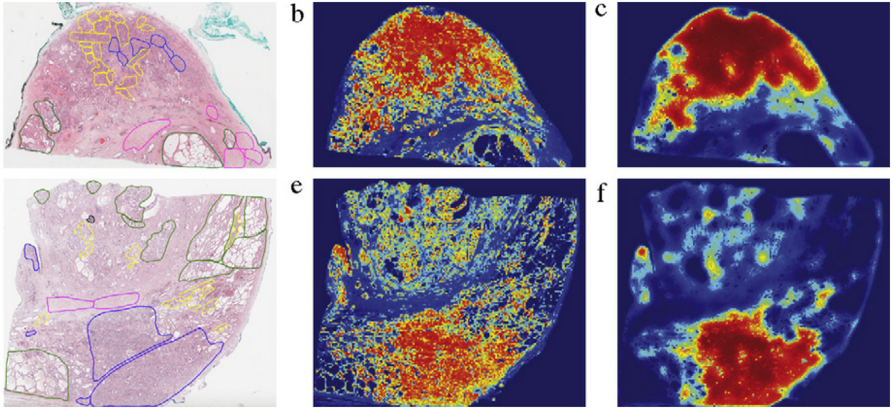
Figure 32: This figure shows the utility of using classification probabilities for heat map visualization at the tile level. There is a good difference between strong positive and negative results (red versus blue). This figure corresponds to Fig.16 in Difranco-2011-ESWS .

In Nayak-2013-CTHS , a method of automatically learning features from unlabeled images is proposed for WSI classification. The first step is to learn the dictionary from the unlabeled images. Then the sparse automatic encoder is used to learn the function. An automatic encoder consists of three parts: an encoder, a dictionary, and a set of codes. The encoder is used to train the classifier on a small amount of label data. Multi-class regularization support vector classification is used, the regularization parameter is 1, and the polynomial kernel is 3. In terms of data, two datasets from (i) glioblastoma multiforme (GBM) and (ii) clear cell renal cell carcinoma (KIRC) of TCGA are used. The classification accuracy rates of $84.3\%$ and $80.9\%$ are obtained respectively. The classification results of heterogeneous GBM tissue sections are shown in Figure. 33.

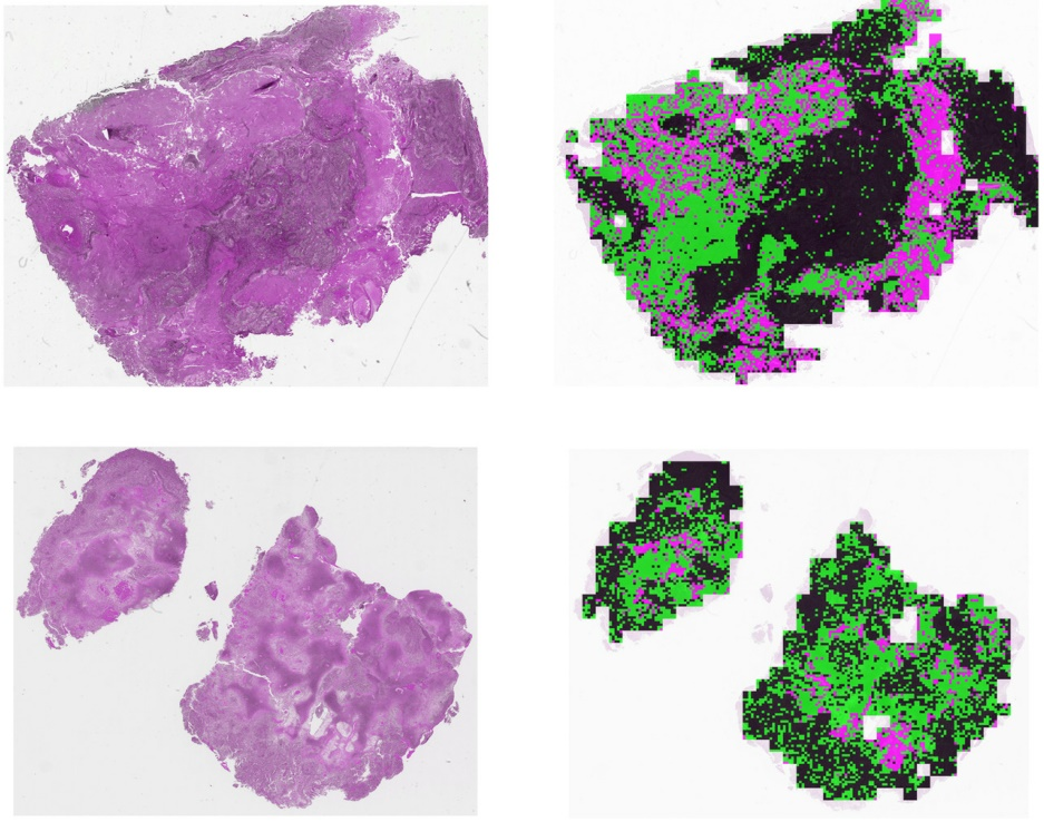
Figure 33: Two examples of classification results of a heterogeneous GBM tissue sections. The left and right images correspond to the original and classification results, respectively. Color coding is black (tumor), pink (necrosis), and green (transition to necrosis). This figure corresponds to Fig.4 in Nayak-2013-CTHS .

In Jiao-2013-CCDU , an SVM based classifier is used to classify colon cancer WSI and non-colon cancer WSI. Then, 18 simple features (such as gray-level mean and gray-level variance) and 16 texture features extracted by the GLCM method are selected as the feature set. The final result shows that when all features are used, the mean values of accuracy, recall and F-measure are $96.67\%$, $83.33\%$, and $89.51\%$, respectively.

In Lu-2015-AADS , a technology for automatically diagnosing skin using WSI is proposed. There are five steps: epidermal segmentation, keratinocyte segmentation, melanocyte detection, feature construction and classification. Based on the segmented ROI, the spatial distribution and morphological features are constructed. A multi-class SVM classifier classifies these features representing skin tissue. It provides about $90\%$ accuracy in the classification of melanoma, and normal skin.

In Weingant-2015-EPTC , the WSI of prostate tumors is classified. First, adaptive cell density estimation is introduced, and H&E staining normalization is applied in the supervised classification framework to improve the robustness of the classifier. RF feature selection, class-balanced training sample sub-sampling, and SVM classification are used to predict high- and low-grade prostate cancer on image slices. AUC measured the classification performance to get 0.703 for HG-PCA and 0.705 for LG-PCA. The results proved the effectiveness of cell density and staining standardization for prostate WSIs classification.

In Peikari-2015-TDRR , a texture analysis technique is proposed to simplify the processing of H&E stained WSIs by classifying clinically important areas. The specific method is to randomly select image blocks from the entire tissue area, divide them into small blocks, and perform Gaussian texture filtering on them. The texture filter responses for each texture are combined and statistical indicators are obtained from the histogram of the response. Then, the visual word bag pipeline is used to combine extracted features to form a word histogram for each image block. The SVM classifier is trained using the computed lexical histograms to distinguish clinically relevant and unrelated plaques. Finally, the ROC is 0.87. It can be proved that texture features can be used to classify important areas in WSI.

In Gadermayr-2016-DACC , to improve the generalization ability of the classification model for kidney WSI, a domain adaptive method is proposed, in which the classifier is trained on the data from the source domain to present a small number of user-labeled samples from the target domain. Efficient linear SVM is used to avoid waiting time during interaction. In a comparison between interactive and non-interactive domain adaptation, it is observed that interactive domain adaptation has a positive effect on the classification performance.

In Shukla-2017-CFRI , SVM is used to predict the presence of cancer by WSI of sentinel lymph nodes, and an equivalent fuzzy model is developed to improve the interpretability. The SVM model consists of 50 support vectors, and the accuracy rate is $94.59\%$. This uses all 50 support vectors to create a fuzzy rule-based model (FRBS) equivalent to two IF-then rules, which categorizes each WSI as non-cancerous and cancerous. FRBS achieved an accuracy rate of $91.89\%$. Experiments show that the work of SVM can be accurately represented in a human interpretable method.

In Xu-2018-AACM , an automatic WSI analysis and classification technology for melanocyte tumors is proposed. First, the skin epidermis and dermis regions are segmented through a multi-resolution frame. Next, an epidermal analysis is performed, in which a set of epidermal features reflecting the nucleus morphology and spatial distribution are calculated. While performing epidermal analysis, dermal analysis is also performed, in which the dermal cell nucleus is segmented, and a set of structural and cytological features are calculated. Finally, by using a multi-class SVM with extracted epidermal and dermal features, the skin melanocyte images are classified into different categories. It is known from the experimental results that the classification accuracy of this technology is over $95\%$.

Random Forest-based Classification Method

RF is a popular machine learning algorithm, often used in classification tasks in various fields  Cutler-2007-RFCE ; Ghimire-2010-CLCC ; Gislason-2006-RFLC ; Guo-2011-RALM ; Chen-2005-PPPI ; Ozccift-2011-RFEC ; Seera-2014-HISM ; Titapiccolo-2013-AIMS . RF is a collection of tree structure classifiers  Breiman-2001-RF . Each tree relies on the value of a randomly selected vector distributed in the same way among all trees in the forest Masetic-2016-CHFD . Each tree in the forest will vote once, assigning each input to the most likely category label. This method is fast and robust to noise, and is a successful ensemble that can identify nonlinear patterns in data. It can easily handle numerical and categorical data Titapiccolo-2013-AIMS . One of the main advantages of RF is that even if more trees are added to the forest, it causes overfitting Chaudhary-2016-IRFC . In the papers we have summarized, there are five papers mainly using RF classifiers for related WSI classification.

In Homeyer-2013-PQNH , it is mainly to quantify the necrotic part in histological WSIs. First, the threshold principle is used to eliminate the background. Color and texture features are then extracted. After the feature classification step is performed, another post-processing step is performed to process the misclassified isolated tiles, that is, using the principle of context classification and spatial context information to re-evaluate all uncertainly classified slices. The sections are then merged, and each section is identified by merging all the non-background slices joined by the edges. Finally, the results are evaluated. Naive Bayes classifier, $k$-nearest neighbor ($k$NN), and RF classifier are used in the post-processing classifier. From the experimental results, it can be known that the RF classifier has the best results, and the HSV-based features are better than RGB.

In Sharma-2016-DCNN , the main task is to automatically classify cancer from histopathological stomach images. The classification performance of traditional image analysis methods and deep learning methods are quantitatively compared. First, the data is augmented. In traditional image analysis methods, the classifier used is a RF classifier.

Metastatic breast cancer is identified in Wang-2016-DLIM . First, the background is automatically detected based on the threshold. And by comparing GoogLeNet, AlexNet, VGG16 and FaceNet. GoogLeNet is selected to generate tumor probability heatmaps, and a RF classifier is used to classify metastatic WSIs and negative WSIs, and finally the AUC of 0.925 is obtained.

In Jamaluddin-2017-TDWS , normal sections and tumor sections from histological images of lymph node tissue are classified. The first step is to remove unnecessary information. The CNN model is then reconstructed or trained to segment the tumor area. The specific details are in Sec. 6. After the tumor area is segmented, the features are extracted, and the RF classifier is used for classification. Finally the result with an AUC score of 0.94 is obtained.

In Klimov-2019-WSIB , the risk of recurrence of DCIS is classified. First of all, the color normalization and down sampling tasks is performed. Secondly, the texture features are extracted. Then, input these features into the RF classifier to predict the high and low risk of recurrence. It is convenient for the doctor to give the corresponding diagnosis and treatment plan. The final result shows that the classifier significantly predicts the 10-year risk of recurrence during training (accuracy = 0.87, sensitivity = 0.71, and specificity = 0.91).

Others Traditional Machine Learning Classification Method

In addition to the two commonly used classification methods of SVM and RF, some other methods are also used to classify histopathological WSI, such as Bayesian classifier Domingos-1997-OSBC and $k$NN Hastie-1996-DANN classifier.

In Sertel-2008-CAPN ; Sertel-2009-CPNW , a system has been developed for quantitative analysis of neuroblastoma WSIs, which included stromal rich and stromal poor. The developed method is based on the Gaussian pyramid method with multi-resolution. WSIs include non-overlapping image blocks and parallel processing of image blocks, which is carried out by the parallel computing module developed previously. Then, the texture features are extracted and the optimal subset is executed. Next, the feature selection of the sequential float forward selection (SFFS) method is adopted, and the confidence degree is calculated by $k$NN classification. If the confidence level falls below the set threshold, switch to a higher resolution. The experimental results show that the overall classification accuracy is $95\%$, and the calculation amount is reduced by $60\%$.

In Kong-2009-CAEN , WSI is graded for neuroblastoma biopsy. The texture features obtained from the segmentation components of the tissue are extracted and processed by an automatic classifier group. This automatic classifier group Multiple Classifiers: $k$NN, linear discriminant analysis (LDA) & $k$NN, LDA & nearest mean (NM), correlation LDA (CORRLDA) & $k$NN, CORRLDA & NM, LDA & Bayesian and SVM with a linear kernel. The output of multiple classifiers is then selected using a simple two-step classifier combination mechanism consisting of voting and weighting processes. The automatic classifier group is trained in multi-resolution frame with different levels of differentiation. The trained classification system is tested on 33 WSIs. Finally, the classification accuracy is $87.88\%$.

In Doyle-2010-BBMC , prostate cancer regions in WSIs are identified. WSIs are first decomposed into an image pyramid with multiple resolution levels. Areas identified as cancer by a Bayesian classifier at a lower resolution are then identified at a higher resolution. At each resolution level, the AdaBoost integration method is used to select 10 image features from more than 900 first order statistical, second order co-occurrence and Gaborfilter feature groups. The experimental result shows that compared with other classifiers, the Bayesian classifier produces higher AUC and precision.

5.2 Deep Learning based Classification Method

In this section, the relevant contents of using deep learning algorithms to classify histopathological images with WSIs are summarized.

In Arevalo-2015-UFLF , basal cell carcinoma WSIs are studied as an integrated unsupervised characteristic. First, a set of feature detectors are learned from a set of patches randomly sampled in the image set. The detectors will capture the most common patterns by simulating the automatic encoder neural network. The image is then represented using the convolution or BOF method. This representation is achieved using the feature detector learned in the previous step. Next, the representation obtained from the convolution or BOF method to train the binary classification model, the softmax regression classifier. Basal cell carcinoma includes different categories of cancer and non-cancer carcinoma. The final result of the system is shown in Figure. 34. The best results in AUC are obtained, which are superior to the most advanced $7\%$ and $98.1\%$.

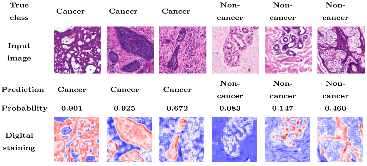
Figure 34: Outputs produced by the system for different cancer and non-cancer input images (red stain indicates cancer regions, blue stain indicates normal regions). This figure corresponds to Table.2 in Arevalo-2015-UFLF .

In Barker-2016-ACBT , brain tumor types in WSIs are automatically classified. The main method is to analyze local features from coarse to fine in pathological images. Firstly, the diversity of rough areas in WSIs is analyzed, including the spatial local characteristics of shape, color, and texture of WSIs. Then the clustering-based method is used to create the representative group. The individual representative tiles in each group are then concretely analyzed. An Elastic Net classifier produces the diagnostic decision value for tile to obtain the WSI level diagnosis. Finally, 302 cases of brain cancer included automatically two possible diagnoses (glioblastoma multiforme (182 cases) and glioblastoma low grade (120 cases)) to evaluate our method with an accuracy rate of $93.1\%$ ($P\ll 0.001$).

In Geccer-2016-DCBC and Gecer-2018-DCCW , deep convolutional networks are used to detect and classify WSIs ROI in breast cancer. The detection part is described in detail in Sec. 6. In this part, the classification is mainly introduced, that is, the ROI include five diagnostic categories. The classifier is designed based on CNN, which uses the features learned by CNN to classify the detected ROI. The CNN structure diagram designed is shown in Figure. 35. Then the post-processing of WSI classification is carried out. WSIs are classified according to the prediction of most categories in the remaining cancer areas. The results show that the efficiency is improved by about 6.6 times with sufficient accuracy.

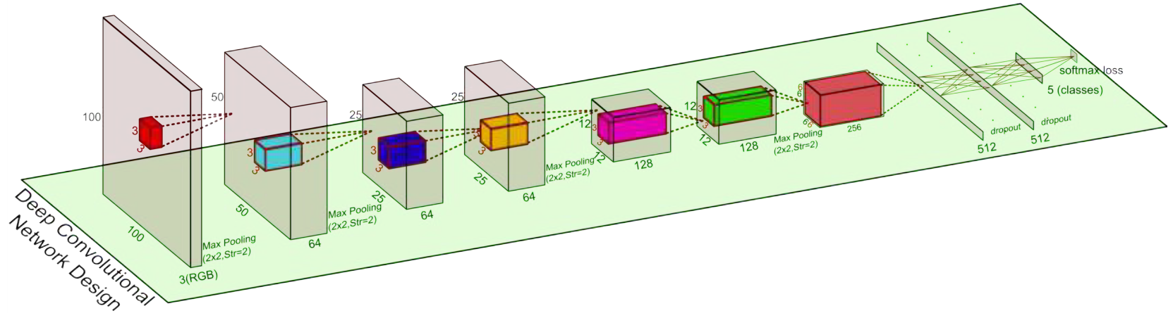
Figure 35: Designs of the CNN. This figure corresponds to Figure.4.6 in Geccer-2016-DCBC .

In Sirinukunwattana-2016-LSDL , it mainly includes two parts, namely, the detection and classification of cell nuclei. The detection part proposes a spatially constrained CNN for nuclear detection. The details are in Sec. 6. Classification uses a new NEP combined with CNN. None of the proposed detection and classification methods require nuclear segmentation. And the proposed method is applied to colorectal adenocarcinoma WSIs, and the final classification result obtains a higher F1 score. The final detection and classification results are shown in the Figure. 36.

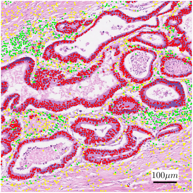
Figure 36: The detection and classification are the result graphs under 20 times magnification. This figure corresponds to Figure.9.(c) in Sirinukunwattana-2016-LSDL .

In Hou-2016-PCNN , an expectation maximization method is proposed. The spatial relationship of patches is used to locate the distinguished patches robustly. This method is applied to the subtype classification of glioma and non-small cell lung cancer. The classification module uses patch-level CNN and trains a decision fusion model as a two-level model. The first level (patch-level) model is based on expectation maximization, combined with CNN output patch-level prediction. In the second level (image-level), the patch-level predicted histogram is input to the image-level multiple logistic regression or SVM.

In Babaie-2017-CRDP , a new dataset, Kimia Path24, is introduced for image classification and retrieval in digital pathology. The WSIs of 24 different textures are generated to test patches. Especially, the patch classification is based on LBP histograms, bag-of-words approach, and CNN.

In Araujo-2017-CBCH , a method to classify WSI for breast biopsies using CNN is proposed. The proposed network architecture can retrieve information on different scales. First, the image includes 12 non-overlapping patches, and then the piece-by-piece training CNN and CNN+SVM classifier are used to calculate the patch-level probability. Finally, one of three different patch probability fusion methods is used to obtain image classification results. These three methods are majority voting (choosing the most common patch as the image tag), maximum probability (choosing the patch category with high probability as the image tag), and probability (the category with the largest sum of patch-level probability). The final results classify the images into four categories: invasive, in situ, benign and normal. The proposed system achieves the overall sensitivity of about $81\%$ of cancer patch classification.

In Bejnordi-2017-CASC , a context-aware stacked CNN is proposed to classify WSIs as normal/benign, DCIS, and invasive ductal carcinoma (IDC). The first is to train a CNN and use high pixel resolution to capture cell level information. The characteristic responses generated by the model are then inputted to the second CNN and superimposed on the first CNN. The system had an AUC of 0.962 for binary classification of non-malignant and malignant slides, and a three-level accuracy rate of $81.3\%$ for normal/benign classification of WSIs, DCIS, and IDC.

In Sharma-2017-DCNN , gastric cancer WSI is automatically classified. The traditional image analysis method and deep learning method are proposed and compared quantitatively. In the traditional analysis method, GLCM, Gabor filter bank response, LBP histogram, gray level histogram, HSV histogram, and RGB histogram are used for classification and RF. In terms of the deep learning method, AlexNet is proposed as a deep convolution framework. The structure of the network is shown in Figure. 37. According to the experiment, the overall classification accuracy of the cancer classification proposed by AlexNet is 0.6990, and the overall classification accuracy of necrosis detection is 0.8144.

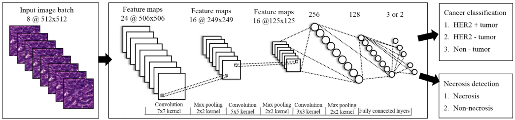
Figure 37: Proposed AlexNet architecture. This figure corresponds to Figure.4 in Sharma-2017-DCNN .

In Korbar-2017-DLCC , different types of colorectal polyps on WSIs are classified to help pathologists diagnose them. Here is a modified version of the ResNet structure. The whole WSI is divided into patches and then applied to the ResNet. If at least five patches on a WSI are recognized as this class, the average confidence level is $70\%$. If there is no cancer type in the patch, the WSI is considered normal. Finally, the accuracy is $93.0\%$. The recall is $88.3\%$; F1 scores $88.8\%$.

In Hu-2017-DLBC , a deep neural network (an 11-layer CNN model) is trained to automatically learn valid features and classify protein images of eight subcellular locations. First, image preprocessing and data balance are carried out. Then, the processed data is passed through the 11-layers of CNN model. Details of the structure are shown in Figure. 38. Finally, the classification accuracy rate reached $47.31\%$ in the test data and $100\%$ in the training data.

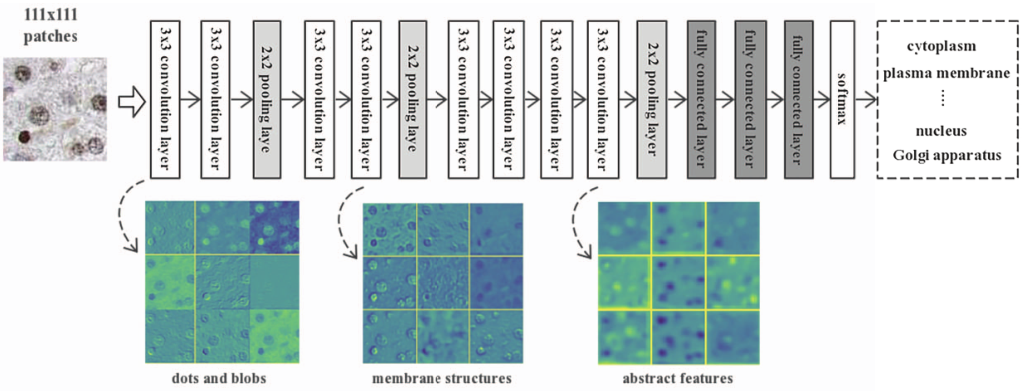
Figure 38: The deep neural network architecture and visualization of intermediate layers features. This figure corresponds to Figure.4 in Hu-2017-DLBC .

In Xu-2017-LSTH , a deep CNN is proposed to conduct large-scale histopathological image classification, segmentation, and visualization. In the part of the classification, WSI is first divided into patches, and background is discarded, and then the selected patches are input into the network to obtain 4096-dimensional CNN feature vectors. The final feature vectors of the image are assembled through softmax. Then feature selection is carried out to remove redundant and irrelevant features. Finally, SVM is used for classification. When using the MICCAI challenge dataset, the classification accuracy is $97.5\%$.

In Korbar-2017-LUHD , an image analysis method based on deep learning is proposed to classify different polyp types on WSIs. This classification model is based on the ResNet architecture, with minor modifications to the architecture. Specifically, replace the last fully connected layer with a convolutional layer. Finally, the average accuracy rate is $91.3\%$, which is better than other deep learning architectures.

In Ghosh-2017-SLCA , a new deep learning method is proposed to classify white blood cells in WSIs. The network uses the average pool level to find the hot spots of the white blood cell location in WSI. The first is to fine-tune the pre-trained AlexNet based on the dataset. Then the network is trained on the patch dataset, and the trained network structure is shown in Figure. 39

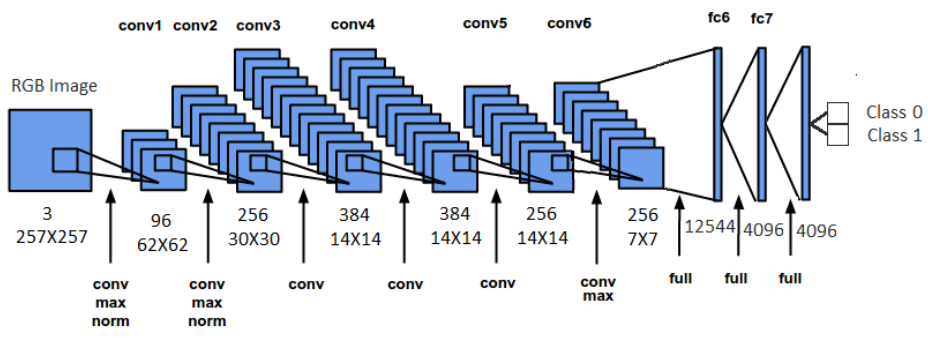
Figure 39: Architecture of the DCN used in approach. This figure corresponds to Figure.1 in Ghosh-2017-SLCA .

In Das-2017-CHWS , a network structure based on CNN is proposed. The tissue section area of WSI is analyzed with multiple resolution methods. That is, the class posterior estimate of each view at a specific magnification is obtained from the CNN at a specific magnification, and then the posterior-estimate of random multiple views at a multiple magnification is voted to filter to provide a slide-level diagnosis. According to the experimental results, the final classification accuracy is $94.67\pm 14.60\%$, sensitivity $96.00\pm 8.94\%$, specificity $92.00\pm 17.85\%$, and F-score of $96.24\pm 5.29\%$.

In Ren-2018-ADAC , prostate histopathology WSI is graded. The main method is an unsupervised domain adaptive method. The adaptation here is achieved through confrontation training, which can minimize the distribution difference of feature space between two domains (annotated source domain and untagged target domain) with the same number of high-level classes. The loss function also uses Generative Adversarial Network (GAN). Besides, a Siamese architecture is also developed to normalize patch in WSIs. A flowchart of the entire method is shown in the Figure. 40. The method is then applied to the public prostate dataset for verification. The experimental results show that this method improves the classification accuracy of the Gleason score significantly.

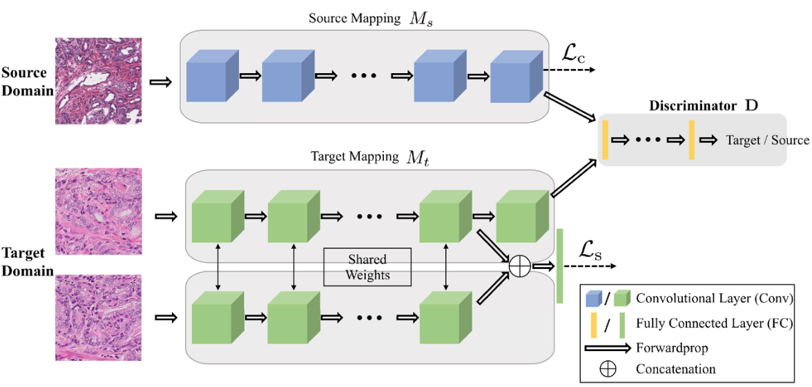
Figure 40: The architecture of the networks for the unsupervised domain adaptation. This figure corresponds to Figure.1 in Ren-2018-ADAC .

In Courtiol-2018-CDLH , a method of classification and localization of diseases with weak supervision is proposed. First, WSIs pretreatments are performed, including foreground and background segmentation, color normalization, and tile partitioning. Then ResNet is used for feature extraction. Then, the WELDON method is proposed by Durand et al. is improved and adjusted Durand-2016-WWSL . Modification of the pre-trained deep CNN model, feature embedding, and introduction of an additional set of full connection layers for context re-classification from instances. The final classification output diagram is generated as shown in Figure. 41.

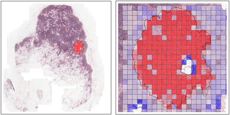
Figure 41: The classification result of the proposed method in Camelyon16 dataset. This figure corresponds to Figure.4 in Courtiol-2018-CDLH .

In Tellez-2018-GWSI , a two-part approach is proposed to classify WSIs. Firstly, the encoder is trained in an unsupervised way, and the tissue blocks on WSI are mapped to the embedded vector, and the sliding window is used to form the stack of the feature map of WSI. Then, the CNN classifier is trained based on the compact representation of WSIs. There are three types of encoders trained here: convolutional autoencoder (CAE), variational autoencoder (VAE) and a new method based on contrast training. Experiments show that the new contrast encoder is superior to CAE and VAE.

In Morkunas-2018-MLBC , WSI colorectal cancer tumor tissue is classified. The simple linear iterative clustering (SLIC) algorithm is proposed by Achanta et al. Achanta-2012-SSCS is mainly applied to generate superpixels, and superpixels are used to annotate the image. Therefore, the selected area is divided into superpixels. Then, color texture features are extracted and dimensionality reduction is used to regenerate composite features. Experiment shows that the superpixel method is suitable for using different classification algorithms based on machine learning.

In Kwok-2018-MCBC , a multi classification of breast cancer in WSI is presented. They propose a deep learning framework, which is mainly divided into two stages, using microscopic images and WSI to achieve the purpose of classification. After the two types of images are patched, the microscopic images are used for Inception- ResNet-v2 to train the classifier. The WSIs are then subsampled and converted from RGB to CIE-LAB color space and segments the foreground from and background. Then the extraction of hard examples and patch classifier is retrained. The prediction results are aggregated from the block by block prediction back to image prediction and WSI annotation. This method is applied to ICIAR 2018 Grand Challenge on breast cancer histology images, with an accuracy rate of $87\%$, far exceeding the second place. The specific working process is shown in Figure. 42.

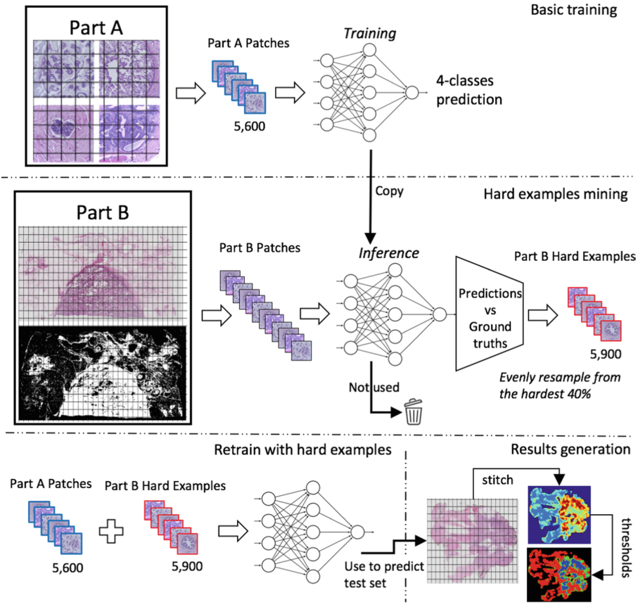
Figure 42: Overview of the framework. This figure corresponds to Figure.1 in Kwok-2018-MCBC .

In Mercan-2017-MIML , a weakly supervised method for multi-classification of breast histopathology WSIs is proposed. Firstly, ROI is extracted by zooming, translation, and fixation. Then, the color and texture information and structural features are extracted in CIE-LAB space. Next, four different multi-instance multi-label (MIML) learning algorithms are used to predict the slide level and ROI level in the image. The result is an average classification accuracy of $78\%$ at slide level 5-Class.

The author in  Das-2018-MILD also proposes a multiple instance learning (MIL) framework based on breast cancer WSI. This framework is based on CNN and introduces a new pooling layer that enables the patch in WSI to aggregate the most informative features. This pooling layer is a new layer of the multi-instance pool (MIP), which introduces MIL as an end-to-end learning process into DNN to realize WSIs classification. At the end, high classification sensitivity of $93.87\%$, $95.81\%$, $93.17\%$, and $88.95\%$ are achieved with four different magnifications using the public dataset.

The study in  Campanella-2018-TSDM is also based on the MIL classification for prostate cancer. Slide tiling is the first run at different magnification and its bags are generated. Then, model training is carried out to find the tiling with the highest positive and negative probability in the slide, which is used to give more importance to the under-representative examples. Then, based on AlexNet, ResNet, VGG classification, given a threshold, if at least one instance is positive, then the WSI is called positive and the slide is negative if all instances are negative. The optimal models are Resnet34 and VGG11-BN, with AUC of 0.976 and 0.977, respectively. The method of Campanella-2019-CGCP is roughly the same as that of Campanella-2018-TSDM .

In Wang-2018-WSLW , a weakly supervised learning approach is used to classify WSI lung cancer. Firstly, the improved FCN based on patch-level from WSI is used for cancer prediction to find the different regions as the prediction model of patch-level. When the probability of a block exceeds the threshold, it is retrieved. Then, context-based feature selection and aggregation from the retrieved parts are performed to construct the global feature descriptor. Finally, the global feature descriptor is input into the standard RF classifier. Finally, a high classification accuracy of $97.1\%$ is obtained.

In Shou-2018-WSIC , CNN is mainly used to classify gastric cancer in WSI. Firstly, the difference of threshold value and color feature is used to extract the tissue and conduct morphological processing. Then, it is separated into patches, and the data is expanded by flipping. Then, the existing CNN architecture is utilized to conduct experiments on patch-level and slide-level. Finally, good results are obtained on DenseNet-201.

In Li-2019-AMRM , a multi-resolution classification of prostate WSIs based on attention mechanism is performed. The MIL model based on attention is used to extract transient features. The overall process is separated into two parts. The first part is to classify cancer and non-cancer, using attention-based clustering tile selection. The second part is to conduct cancer classification research with higher resolution. Finally, an average classification accuracy rate of $85.11\%$ is obtained, and the new performance of prostate cancer classification is realized.

In Wang-2019-RRMI , multi-instance deep learning is also used to classify WSI gastric cancer images. A method named RMDL method is proposed. Similar to the above MIL method, it separated into two stages. The first phase also trains a localization network to select the discriminative instances. In the second stage, the RMDL network is used for image-level label prediction. The network is composed of local-global feature fusion, instance recalibration, and multi-instance pooling modules. The specific working process is shown in Figure. 43.

Figure 43: Overview of the framework. This figure corresponds to Figure.2 in Wang-2019-RRMI .

5.3 Others Classification Method

Among the papers we have reviewed, seven papers are based on classification Diamond-2004-UMCT ; Harder-2016-CFCG ; Petushi-2006-LSCH ; Sertel-2009-CCCS ; Yeh-2014-MSDP ; Yoshida-2017-AHCWC ; Yoshida-2018-AHCWG , and they involve techniques related to machine learning.

In Diamond-2004-UMCT , a machine vision system is developed, which uses its morphological features and texture analysis to classify the sub-regions in WSIs. However, it focuses on the application of features and does not introduce the classification part of the machine vision system in detail. The study in  Harder-2016-CFCG also do not make a special description of the classifier, but only focused on the features.

In Petushi-2006-LSCH , the LNKNET software package is used to classify breast cancer WSIs. LNKNet integrates neural networks, statistical and machine learning classification, clustering, and feature selection algorithms into a modular package.

In Sertel-2009-CCCS , a classification framework is proposed to classify the degree of neuroblastoma differentiation. The main point here is that a new method of structuring structural features are introduced, and its classification method is also based on probability, namely mapping decision rules.

In Yeh-2014-MSDP , the pixel-based stain classification is carried out to classify the IHC stain and the nearest neighbor classification, mainly using the nearest neighbor and morphological methods. Then, the density distribution of the identified IHC stains are calculated by the kernel density estimator. After that the staining distribution on WSI is obtained.

Both Yoshida-2017-AHCWC and  Yoshida-2018-AHCWG are used to evaluate the classification accuracy of an automated image analysis system, E-pathologist. Among them, Yoshida-2017-AHCWC is for colorectal biopsy, and Yoshida-2018-AHCWG is for gastric biopsy.

5.4 Summary

From what we have summarized above, we can see that the combination of CAD and WSI technology is used for classification methods, including traditional machine learning methods, deep learning methods, and some other methods.

In traditional machine learning algorithms, the commonly used algorithms used in WSI classification are SVM and RF. There are other algorithms, such as $k$NN. Since 2008, traditional machine learning algorithms have taken the mainstream position in WSI classification. In 2015, deep learning algorithms began to be widely used, obtaining classification results with higher accuracy than traditional machine learning algorithms. Among them, MIL has many applications. Table. LABEL:SCMC is a summary of the CAD method of classification technology in WSI.

Table 6: Summary of the CAD methods used for classification in WSI.

Method	Reference	Year	Team	Details
SVM	Difranco-2011-ESWS	2011	Matthew D. DiFranco	RF, linear SVMs, RBF SVMs are used to classify a collection of 19 B * channel features
SVM	Nayak-2013-CTHS	2013	Nandita Nayak	Multi-class regularized SVM classification with regularized parameters 1 and 3 polynomial kernels
SVM	Jiao-2013-CCDU	2013	Liping Jiao	SVM
SVM	Lu-2015-AADS	2015	Cheng Lu	SVM
SVM	Weingant-2015-EPTC	2015	Michaela Weingant	RF feature selection, class balance training sample subsampling and SVM classification
SVM	Peikari-2015-TDRR	2015	Peikari M	An SVM with a RBF kernel
SVM	Gadermayr-2016-DACC	2016	Gadermayr M	The efficient linear C-SVM
SVM	Shukla-2017-CFRI	2017	Shukla P	SVM
SVM	Xu-2018-AACM	2018	Hongming Xu	MSVM
RF	Homeyer-2013-PQNH	2013	André Homeyer	Naive Bayes classifier, $k$NN classifier, RF classifier
RF	Sharma-2016-DCNN	2016	Sharma H	$\backslash$
RF	Wang-2016-DLIM	2016	Dayong Wang	The post processing uses the RF classifier for classification
RF	Jamaluddin-2017-TDWS	2017	Jamaluddin M F	$\backslash$
RF	Klimov-2019-WSIB	2019	S Klimov	$\backslash$
$k$NN	Sertel-2008-CAPN	2008	Olcay Sertel	A multi-resolution classification system is developed based on the improved $k$NN classifier
$k$NN	Sertel-2009-CPNW	2009	O Sertel, J Kong	Multi-resolution decomposition of training images is performed by Gaussian pyramid method, and improved $k$NN
Bayesian	Doyle-2010-BBMC	2012	Scott Doyle	Strong Bayesian multi-resolution classifier
Mixed classifiers	Kong-2009-CAEN	2009	J Kong, O Sertel	A simple two-step classifier combination mechanism consisting of voting and weighting processes is chosen to aggregate the output of multiple classifiers.
DL	Arevalo-2015-UFLF	2015	John Arevalo	Softmax,Linear-SVM
DL	Barker-2016-ACBT	2016	Barker J	Elastic Net classifier
DL	Geccer-2016-DCBC	2016	Geçer B	CNN
DL	Sirinukunwattana-2016-LSDL	2016	Sirinukunwattana K	NEP is combined with CNN
DL	Hou-2016-PCNN	2016	Hou L	CNN,EM algorithm, SVM
DL	Babaie-2017-CRDP	2017	Babaie M	Applied LBP, the dictionary approach and CNNs to classify patches
DL	Araujo-2017-CBCH	2017	Araújo T	CNN
DL	Bejnordi-2017-CASC	2017	Bejnordi B E	Contextual Awareness Stacked CNN
DL	Sharma-2017-DCNN	2017	Sharma H	The AlexNet deep convolutional comparison with RF is made, and a CNN architecture is proposed
DL	Korbar-2017-DLCC	2017	Korbar B	Resnet
DL	Hu-2017-DLBC	2017	Hu J X	CNN
DL	Xu-2017-LSTH	2017	Xu Y	CNN
DL	Korbar-2017-LUHD	2017	Korbar B	ResNet
DL	Ghosh-2017-SLCA	2017	Ghosh A	AlexNet
DL	Das-2017-CHWS	2017	Das K, Karri S P K	CNN
DL	Ren-2018-ADAC	2018	Jian Ren	Siamese neural network and GAN network
DL	Courtiol-2018-CDLH	2018	Courtiol P	Modify the pre-trained DCNN model to introduce an additional set of full connection layers for context reclassification from instances
DL	Gecer-2018-DCCW	2018	Baris Gecer	CNN
DL	Tellez-2018-GWSI	2018	David Tellez	CNN
DL	Morkunas-2018-MLBC	2018	Morkūnas M	CNN
DL	Kwok-2018-MCBC	2018	Scotty Kwok	Inception-Resnet-v2
DL	Mercan-2017-MIML	2018	Caner Mercan	MIML framework
DL	Das-2018-MILD	2018	Kausik Das	Based on VGG
DL	Campanella-2018-TSDM	2018	Campanella G	AlexNet, VGG11-BN, ResNet18, ResNet34 (MIL)
DL	Wang-2018-WSLW	2018	X Wang	CNN (find discriminative region) RF (classification)
DL	Shou-2018-WSIC	2018	Junni Shou	CNN
DL	Li-2019-AMRM	2019	Jiayun Li	Attention-based clustering and CNN
DL	Campanella-2019-CGCP	2019	Gabriele Campanella	CNN RNN
DL	Wang-2019-RRMI	2019	Shujun Wang	New RMDL network
Others	Diamond-2004-UMCT	2004	JamesDiamondPhDa	A machine vision system is developed, but the emphasis is on the application of features
Others	Petushi-2006-LSCH	2006	Sokol Petushi	LNKNET package
Others	Sertel-2009-CCCS	2009	O Sertel	Classified according to the distance between classes and the distance between classes
Others	Yeh-2014-MSDP	2014	Fang‑Cheng Yeh	Classification to calculate IHC stain density distribution
Others	Harder-2016-CFCG	2016	Harder N	Emphasis is on the application of features
Others	Yoshida-2017-AHCWC	2017	Yoshida H	Compare human pathologist and E-Pathologist
Others	Yoshida-2018-AHCWG	2018	Hiroshi Yoshida	E-Pathologist

Table 6: Continue: Summary of the CAD methods used for classification in WSI(Deep learning (DL)).

6 Detection Methods

To completely understand an image, one should accurately estimate the objects’ concept and location in each image Zhao-2019-ODDL . Detection determines whether one or more specific category instances exist in an image or not Vedaldi-2009-MKOD . Detection can provide valuable information for various fields. For example, remote sensing image detection Zhang-2013-HRSI can provide useful information related to geology, meteorology, water conservancy, and face recognition Hsu-2002FDCI . It is widely used in military and public security criminal investigations, and biomedical image detection Szczypinski-2017MFBI make it convenient for doctors in clinical diagnosis and pathological research.

As one of the most common tasks for CAD pathologists to view WSI, the detection method has developed rapidly in recent years. Figure. 2, the number of detection cases is increasing from 2009 to 2019, which reflects the development of detection technology. Besides, the basic content of the CAD view WSI detection method is shown in Figure. 44. As shown in Figure. 44, all CAD WSI methods for disease detection can be roughly divided into three categories. The first category is traditional detection methods (such as SVM, image enhancement, etc.), the second category is an ensemble learning method, and the last category is deep learning method.

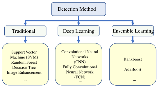
Figure 44: The structure of diseases detection methods in CAD.

6.1 Traditional Detection Method

In this part, we select the traditional detection methods that appear in the papers and summarize these methods.

6.1.1 SVMs based Detection Methods

In Jiao-2013-CCDU , colon cancer is detected by WSI, use SVM to develop a classifier, and select 18 simple features (such as gray-level variance and gray-level mean) and 16 texture features (such as GLCM) to form features. Finally, the experiment uses 3-fold cross-validation and achieves an average precision of $96.67\%$, recall of $83.33\%$, and F-measure of $89.51\%$.

In Sharma-2015-ABND , the texture feature is extracted to represent the necrotic area in the tissue, and the complex dataset is subjected to differentiated threshold processing and SVM is used for machine learning. In the end, the average cross-validation rate is $85.31\%$. It detects the heterogeneity of necrosis in WSI effectively.

In Han-2018-ACDL , calculate the tissue composition map of the WSI and extract the first-order and second-order texture features. Using SVM for machine learning, the offline area of the work area is 0.95.

In Simon-2018-MRLF , detect glomeruli on WSI of thin kidney tissue biopsy, LBP feature vector adaptation is used to train the SVM model, the experimental results have obtained high precision ($\textgreater 90\%$) and reasonable recall rate ($\textgreater 70\%$).

In Swiderska-2015-TMMH , WSI is used to determine the sample map and calculate the texture features of each sample pixel and its surroundings, and use SVM classifier to learn, divide the pixels into normal areas and bleeding areas, and then detect in WSI by applying threshold method and extended area minimum method in the area of tumor proliferation, the experimental result shows that automatic evaluation is better than manual evaluation.

In Nguyen-2011-PCDF , since there is no previous information about cancer, a fusion of cell and structural features are used, and a patch-based method is used to detect prostate cancer using an SVM classifier with a RBF and a parameter c of 1. When the threshold is 90 pixels, it provides the most satisfactory detection results (TPR = $78\%$, FPR = $6\%$).

6.1.2 RF based Detection Methods

In Valkonen-2017-MDWS , the WSI rough segmentation simplifies the background, and the color is normalized, the adaptive threshold method is used to obtain the binary image. Moreover, the watershed method is used to divide the nucleus. Then, LBP features are extracted. After, different models are used for metastasis detection. According to the experimental results, the RF achieves an AUC value of 0.97.

In Litjens-2015-ADPC , the SLIC algorithm is used to calculate superpixels, and after removing the pixel background, the color and LBP features of the remaining tissue pixels are calculated. Then, the RF classifier is used to detect the superpixels that are most likely to be cancer, and use the RF to input the highest resolution graphics and gland features to detect the area that may have cancer. The experimental result The experimental result obtaines an AUC of 0.96, and reaches 0.4 specificity at 1.0 sensitivity.

In Bejnordi-2015-MSSC , Similar to  Litjens-2015-ADPC , both use the multi-scale superpixel classification method. The experimental result of detecting breast cancer is that the ROC is 0.958, and the AUC for the tile analysis in comparison is 0.932. In  Bejnordi-2016-ADDW , similar to Litjens-2015-ADPC and Bejnordi-2015-MSSC , it detects DCIS in the WSIs of breast histopathology.

In Li-2015-FRID , the superpixel classification method is also used to obtain the initial recognition of the ROI by gathering superpixels at low magnification. Then, by marking the corresponding pixels, the superpixels are mapped to the higher magnification image. This process is repeated several times until the segmentation is stable. Finally, the RF classifier and SVM respectively mark the superpixels represented by the selected features and quickly detect the ROI in the WSI. Experiments prove that the superpixel results suggested in the article are better than SLIC and non-superpixel.

6.1.3 Other Traditional Detection Methods

There is an article each using DT classifier, clustering algorithm, linear discriminator and machine learning organization classifier Lopez-2013-ABDM ; Lopez-2012-CMAD ; Veta-2013-DMFB ; Shirinifard-2016-DPAU .

The author in  Lopez-2013-ABDM uses the multiple sharpness feature method to identify the blur area on the WSI. Using different blur features (such as features related to the co-occurrence matrix and image gradient), the best blur detection results are obtained by using a DT classifier (i.e., $98.56\%$ and $96.63\%$ classification accuracy and small hardware investment).

In Lopez-2012-CMAD , Ki67 immunohistochemistry-based WSI technology is used to detect tumor areas with high proliferation activity, a hybrid clustering method, referred to as Seedlink, is developed in the paper. This tool greatly improves the pathologist’s identification of hot-spots consistency.

In Veta-2013-DMFB , the author uses the level set method to extract candidate objects, and use two sets of features (the baseline set describing the size, shape, and color of the extracted candidate objects and the extension of texture information in addition to the baseline set) input into the linear discriminator, divide candidate objects into mitotic figures or fake objects to detect mitosis.

In Shirinifard-2016-DPAU , the staining and texture characteristics of Ki67 stained glass slides is used to divide the tissues in WSI into living tumor tissue, necrotic tissue, and background. And use a tissue classifier based on machine learning, which is trained five times magnified images to be applied to living tumor tissue to detect phenotypic changes. In the end, an accuracy of $95\%$ in each area is achieved.

We found three papers about non-machine learning. In Bautista-2009-DTFW , by introducing a movement operator, it can effectively amplify the chromaticity difference between tissue folds and other tissue components to detect tissue folds in WSI. In Bautista-2010-IVDT , similar to Bautista-2009-DTFW , the weighted difference between the color saturation and brightness of the image pixels is used as the offset factor of the original RGB color of the image to enlarge tissue folds.

In Vyas-2016-CWSD , the author compares the histopathological characteristics of dermatitis cases detected by WSI and traditional microscopy. Although WSI is not as effective as traditional microscopes, it is sufficient to examine the pathological features often encounter in dermatitis cases and get the effect that can be used.

6.2 Deep Learning based Detection Methods

In this section, the relevant content of using deep learning algorithms to detect histopathological images with WSI is briefly summarized.

6.2.1 CNN-based Deep Learning Detection Method

The following Zanjani-2018-CDHW ; Cruz-2017-ARIB ; Bejnordi-2017-DADL ; Tellez-2018-WSMD ; Kohlberger-2019-WSIF ; Jamaluddin-2017-TDWS ; Cruz-2014-ADID are all detection classifiers based on CNN. In Zanjani-2018-CDHW , CRF is applied to the latent space of the trained deep CNN, and the compact features extracted from the middle layer of the CNN are regarded as observations in the fully connected CRF model to detect invasive breast cancer. Experiments show that the average FROC score of tumor area detection in histopathology WSIs increased by about $3.9\%$. The proposed model is trained on the Camelyon17 ISBI challenge dataset and won second place with a kappa score of 0.8759.

In Cruz-2017-ARIB , involved images from five different cohorts from different institutions/ pathologylabs in the United States of America and TCGA. The training dataset had 349 estrogen receptor-positive (ER+) invasive breast cancer patients. The approach yielded a Dice-coefficient of $75.86\%$, a positive predictive value of $71.62\%$ and a negative predictive value of $96.77\%$ in terms of pixel-by-pixel evaluation compared to manually annotated regions of IDC.

In Bejnordi-2017-DADL , the author evaluates the performance of automated deep learning algorithms in detecting metastasis in lymph node H&E tissue sections of women with breast cancer and compares it with a pathologist’s diagnosis in a diagnostic environment. The dataset is collected from 399 patients who underwent breast cancer surgery at the Radboud University Medical Center (RUMC) and Utrecht University Medical Center (UMCU) in the Netherlands. The algorithm in the paper is significantly better than the pathologist’s artificial algorithm.

In Tellez-2018-WSMD , a method for training and evaluating CNNs in breast cancer WSIs mitosis detection is proposed. In the three tasks challenged by Tupac, the performance of the proposed method is independently evaluated.

In Kohlberger-2019-WSIF , an autofocus quality detector called ConFocus is developed to detect and quantify the out-of-focus area and severity on WSIs. When compared to pathologist-graded focus quality, ConvFocus achieved Spearman rank coefficients of 0.81 and 0.94 on two scanners and reproduced the expected OOF patterns from Z-stack scanning. The article also evaluates the impact of OOF on the accuracy of the most advanced metastatic breast cancer detector, and finds that as OOF increases, the performance continues to decline.

Jamaluddin-2017-TDWS is divided into two parts. The first part is to use CNN to detect possible tumor locations in WSI, and the second part is to use the detected results to extract features to classify normal or tumors. Using Camelyon16 dataset, which consists of 160 negatives and 110 positives WSIs for training, and 50 positives and 80 negatives for testing. The method has a better AUC result at 0.94 than the winner of Camelyon16 Challenge with an AUC of 0.925. The CNN structure designed in  Jamaluddin-2017-TDWS is shown in Figure. 45.

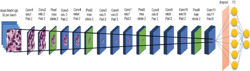
Figure 45: 12 convolutional layer including the fully connected layer. This model was also inspired from VGG model.

In Cruz-2014-ADID , CNN is trained to detect IDC in WSI. At the end, $71.80\%$ of F-measure (F1) and $84.23\%$ of balanced accuracy are obtained. The overall detection framework of Cruz-2014-ADID is shown in Figure. 46.

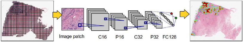
Figure 46: Overall detection framework of  Cruz-2014-ADID .

6.2.2 FCN-based deep learning detection method

The following Geccer-2016-DCBC ; Gecer-2018-DCCW ; Lin-2018-SFDS ; Lin-2019-FSFD are processed with 4-layers of FCN to achieve the purpose of detection.

The study in  Geccer-2016-DCBC is composed of two tasks, retrieval and classification. The retrieval part is composed of four layers of FCN. Through the feedforward processing of FCN-1, the salient area is detected from WSI, and each connected component above the threshold is enlarged on the input image and processed by FCN-2. This process lasts four times, and a significant area of WSI can be detected. Then CNN classifies and finally determines the breast cancer diagnosis results.

In Gecer-2018-DCCW , a system is proposed for diagnosing WSI of breast biopsy. Firstly, four FCNs are used for saliency detection and multi-scale localization of ROI. Then, convolutional network is used for cancer classification. Finally, the saliency map and the classification map are combined. The test result shows that its accuracy rate is roughly indistinguishable from the pathologist’s prediction.

In Lin-2018-SFDS , an improved FCN layer is used to input the WSI of any size, and the standard FCN layers are converted into the anchor layer. Fast and dense ScanNet inference with the anchor layer makes the network faster. The result of its detection of cancer metastasis shows excellent performance on the Camelyon16 Challenge dataset.Similar method is applied in  Lin-2018-SFDS and  Lin-2019-FSFD .

6.2.3 Other deep learning detection methods

The following references Cruz-2018-HTAS ; Sirinukunwattana-2016-LSDL ; Bilaloglu-2019-EPCW are used for detection after combining or simplifying the CNN structure with other methods.

In Cruz-2018-HTAS , a new type of efficient adaptive sampling based on probability gradient and quasi-Monte Carlo sampling is used, combined with a CNN-based classifier. Applied to the detection of invasive breast cancer on WSI. The experimental result shows that the Dice-coefficient is $76\%$, which is an efficient strategy.

In Sirinukunwattana-2016-LSDL , in conventional colon cancer WSI proposes a space-constrained CNN for nuclear detection. The new NEP is used in conjunction with CNN to more accurately predict the type of cell detection. The test result shows that this article produces an higher average F1 score of detection.

In Bilaloglu-2019-EPCW , a simplified CNN, named PathCNN, is used to detect outliers of WSI in whole cancer. The WSI used in the experiment is downloaded from the genome data sharing database of the TCGA.

In Liu-2019-AIBC , Lymph Node Assistant (LYNA), a tool for breast cancer lymph node metastasis detection based on Inception-v3, is evaluated for its application and clinical practice. The data is obtained from two sources: the Camelyon16 challenge containing 399 slides, and a private dataset containing 108 slides from 20 patients (86 tissue blocks). When applying the second dataset, LYNA achieved an AUC of $99.6\%$.

6.3 Ensemble Learning based Detection Method

This section provides a summary of the contents related to the use of WSIs by the ensemble learning algorithm to detect histopathological images.

In Huang-2017-AHGP , the image is sampled based on the kernel density, and the taint deconvolution and feature description are used to extract image features. Then, an enhanced version of the rank boost integrated method (using multiple weak classifiers to obtain better performance of the final rank) is utilized to rank and detect high-level prostate cancer. The experiment shows the mean AUC is $0.9486\pm 0.005$ and the mean accuracy achieves $95.57\%\pm 2.1\%$.

In the first step in Doyle-2010-BBMC , WSIs are decomposed into an image pyramid containing multiple resolution levels. At a lower resolution level, the Bayesian classifier identified the infected areas like cancer, and then a higher resolution level is used for more detailed examination. At each resolution level, the AdaBoost ensemble method is used to collect more than 900 first-order statistics, ten image features are selected from the second-order co-occurrence and Gaborfilter feature pool, and an enhanced Bayesian multi-resolution (BBMR) system is used to detect the coronary artery lesion area on the digital biopsy slice.

6.4 Summary

Among the papers we have summarized, it can be divided into traditional detection methods, detection methods based on deep learning, and detection methods based on ensemble learning.

There are traditional machine learning algorithms and some non-machine learning algorithms in traditional detection methods. Among the traditional detection method, six articles Jiao-2013-CCDU ; Sharma-2015-ABND ; Han-2018-ACDL ; Simon-2018-MRLF ; Swiderska-2015-TMMH ; Nguyen-2011-PCDF use SVM methods and five articles Valkonen-2017-MDWS ; Litjens-2015-ADPC ; Bejnordi-2015-MSSC ; Bejnordi-2016-ADDW ; Li-2015-FRID use RF, DT, clustering, linear discriminator, and organization classifier algorithms. Two non-machine learning papers Bautista-2009-DTFW ; Bautista-2010-IVDT construct a color transfer factor to enhance the image folds for detection. There are 15 papers Zanjani-2018-CDHW ; Cruz-2017-ARIB ; Bejnordi-2017-DADL ; Tellez-2018-WSMD ; Kohlberger-2019-WSIF ; Jamaluddin-2017-TDWS ; Cruz-2014-ADID ; Cruz-2018-HTAS ; Sirinukunwattana-2016-LSDL ; Liu-2019-AIBC ; Geccer-2016-DCBC ; Gecer-2018-DCCW ; Lin-2018-SFDS ; Lin-2019-FSFD related to detection based on deep learning, most of which use CNN. In  Huang-2017-AHGP ; Doyle-2010-BBMC , an ensemble learning based detection, one uses RankBoost and the other uses AdaBoost. It can be seen from the summary paper that before 2010, traditional non-machine learning algorithms are used for detection. Since 2011, machine learning has entered the public arena, and methods such as SVM and RF have been widely used. Until 2016, the emergence of deep learning enables better results. From the detection results, we can also see that CNN obtain high accuracy. Table. LABEL:SCAD is a summary of the CAD methods used for detection in WSI.

Table 7: Summary of the CAD methods used for detection in WSI (Traditional (T), Deep learning (DL), Ensemble Learning (EL), Breast Cancer Surveillance Consortium (BCSC)).

Type	Reference	Year	Team	Data	Details
T	Nguyen-2011-PCDF	2011	Kien Nguyen	$\backslash$	SVM with RBF kernel and c $=$ 1
T	Jiao-2013-CCDU	2013	Liping Jiao	$\backslash$	SVM
T	Sharma-2015-ABND	2015	Harshita Sharma	$\backslash$	SVM
T	Swiderska-2015-TMMH	2015	Zaneta Swiderska	$\backslash$	SVM with Gaussian kernel function
T	Han-2018-ACDL	2018	W. Han	$\backslash$	SVM
T	Simon-2018-MRLF	2018	Olivier Simon	$\backslash$	SVM
T	Litjens-2015-ADPC	2015	Litjens, G	$\backslash$	RF
T	Li-2015-FRID	2015	Ruoyu Li	NLST	RF
T	Bejnordi-2015-MSSC	2015	Bejnordi, B. E	$\backslash$	RF
T	Bejnordi-2016-ADDW	2016	Bejnordi, B. E	$\backslash$	RF
T	Valkonen-2017-MDWS	2017	Valkonen M	$\backslash$	RF
T	Bautista-2009-DTFW	2009	PA Bautista	Massachusetts General Hospital	Color shift factor
T	Bautista-2010-IVDT	2010	PA Bautista	Massachusetts General Hospital	Color shift factor
T	Veta-2013-DMFB	2012	M. Veta	UMCU	Linear discriminator
T	Lopez-2012-CMAD	2012	Lopez X M	$\backslash$	A hybrid clustering method
T	Lopez-2013-ABDM	2013	Lopez X M	$\backslash$	DT
T	Shirinifard-2016-DPAU	2016	Shirinifard A	$\backslash$	A tissue classifier based on machine learning
T	Vyas-2016-CWSD	2016	Vyas N S	$\backslash$	Compare WSI and traditional microscopy
DL	Cruz-2014-ADID	2014	Angel Cruz-Roa	$\backslash$	CNN
DL	Jamaluddin-2017-TDWS	2017	Jamaluddin M F	Camelyon16	CNN
DL	Bejnordi-2017-DADL	2017	Bejnordi, B. E	RUMC and UMCU	CNN
DL	Cruz-2017-ARIB	2017	Angel Cruz-Roa	TCGA	CNN
DL	Zanjani-2018-CDHW	2018	Farhad Ghazvinian Zanjani	Camelyon17	CNN
DL	Tellez-2018-WSMD	2018	David Tellez	TNBC,TUPAC	CNN
DL	Kohlberger-2019-WSIF	2019	T. Kohlberger	$\backslash$	CNN
DL	Geccer-2016-DCBC	2016	Geçer B	$\backslash$	FCN
DL	Gecer-2018-DCCW	2018	Geçer B	registries associated with the BCSC Consortium	FCN
DL	Lin-2018-SFDS	2018	Huangjing Lin	Camelyon16	FCN
DL	Lin-2019-FSFD	2019	Huangjing Lin	Camelyon16	FCN
DL	Sirinukunwattana-2016-LSDL	2016	Sirinukunwattana K	$\backslash$	New NEP is used in conjunction with CNN
DL	Cruz-2018-HTAS	2018	Angel Cruz-Roa	HUP,CWRU,CINJ,TCGA	CNN and adaptive sampling
DL	Bilaloglu-2019-EPCW	2019	S Bilaloglu	TCGA	PathCNN
DL	Liu-2019-AIBC	2019	Liu Y	Camelyon16, a separate dataset	LYNA (Based on Inception-v3)
EL	Doyle-2010-BBMC	2010	S. Doyle	$\backslash$	AdaBoost
EL	Huang-2017-AHGP	2017	Huang C H	TCGA	Rankboost

Table 7: Continue: Summary of the CAD methods used for detection in WSI.

7 Methodology Analysis

This section analyzes prominent methods in different tasks.

7.1 Analysis of Segmentation Applications in WSI

In recent years, medical WSIs have been used for segmentation to assist doctors in their diagnosis and treatment. Most of them use deep learning algorithms. Because of the different datasets used in each effort, it is impossible to evaluate each segmentation method’s effectiveness vertically. The use of multi-resolution U-net architecture is undoubtedly a common one, as shown in Figure. 47.

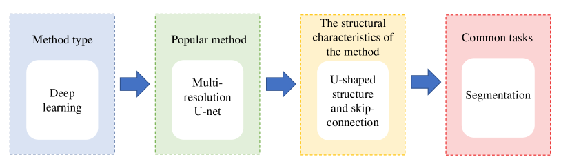
Figure 47: The popular methods for segmentation in WSIs.

Its U-shaped structure and its skip-connection are its structural characteristics. The U-shaped structure can be used to extract deep features by down-sampling and down-dimension-reduction, and then up-sampling to obtain more accurate output images. This kind of end-to-end network can achieve good results in medical image segmentation. There is another multi-resolution encoder-decoder network for breast cancer segmentation Mehta-2018-LSBB , which is similar to the U-net method. However, U-net structure can only be predicted on a single scale, so it cannot cope with scale changes well. Moreover, training does not have good generalization ability when the convolutional layer is increased Du-2020-MISU . Breast cancer is the most commonly used Dong-2018-RANT ; Mehta-2018-LSBB ; Apou-2014-FSTC ; Veta-2013-ANSH ; Veta-2012-PVAE ; Roullier-2010-GMRS ; Roullier-2010-MEBC ; Seth-2019-ALBD ; Seth-2019-ASDW tasks in segmenting WSI to assist pathologists in diagnosis.

7.2 Analysis of Classification and Detection Applications in WSI

According to the review of classification applications of WSI in CAD, it can be seen that SVM is the most frequently used technique in traditional machine learning. However, basic SVM cannot achieve excellent classification results. For example, in Nayak-2013-CTHS , multi-class regularized SVM is used to classify tumors, and the accuracy rate is only $84\%$. In Peikari-2015-TDRR , the RBF SVM is used for classification, and only 0.87 AUC is obtained. However, if SVM is combined with SVM of other kernel functions or other kinds of classifiers to train ensemble learning classifiers, the results will be highly improved. For example, in Difranco-2011-ESWS , the AUC of prostate cancer is 0.95 when it is classified. However, this ensemble learning method has low efficiency, slow running speed, and requires a large number of parameters. For some more complex tasks, a large number of calculations are needed Weihua-2013-RCMA .

In the traditional machine learning algorithm, the Gaussian pyramid method is also commonly combined with $k$NN to improve the classification accuracy. The Gaussian pyramid is based on simple down-sampling plus Gaussian filtering. The original image is continuously sampled by decreasing order, and a series of images of different sizes are obtained, from large to small, from bottom to top, to form a tower model. In this way, images of different resolutions can be obtained, thus improving the accuracy of classification. For example, in Sertel-2008-CAPN , the improved $k$NN combined with the Gaussian pyramid is used to classify neuroblastoma, and the classification accuracy of $95\%$ is obtained. However, in the classification problem of unbalanced datasets, the defects of $k$NN are obvious. Due to the influence of sample distribution, the minority class will be more biased towards the majority class discrimination Li-2011-IKNN .

In the deep learning classification algorithm, most of them are based on CNN. CNN is better than traditional machine learning methods in processing high-dimensional data, and because of the convolutional layer, it can automatically extract features for learning. In recent years, MIL and neural networks are often used to carry out classification tasks for medical WSIs. For example Mercan-2017-MIML ; Das-2018-MILD ; Campanella-2018-TSDM ; Campanella-2019-CGCP ; Wang-2019-RRMI . MIL is a learning problem with Multiple example packages as training units. A bag is marked as a positive-class multi-example package if it contains at least one positive instance. Conversely, the negative example is also true. The multi-example learning method can effectively reduce the noise and improve the classification accuracy of the prediction. In Campanella-2018-TSDM ; Campanella-2019-CGCP , the AUC of its classification is 0.98, a good result. However, the CNN-based neural network is an end-to-end architecture, similar to a black box, which is weak in interpretation Zhang-2013-CML . The popular methods in classification for WSIs are as shown in Figure. 48.

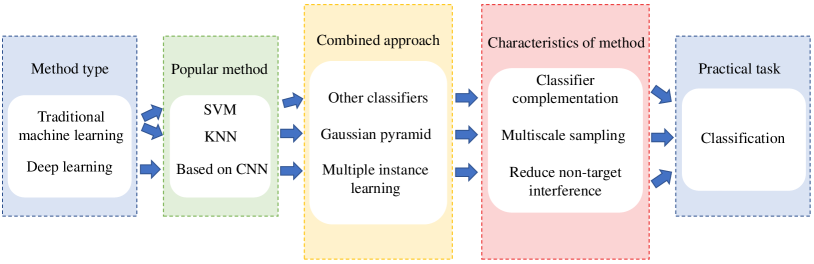
Figure 48: The popular methods in classification for WSIs.

In the task of WSIs classification, the classification of breast cancer Peikari-2015-TDRR ; Wang-2016-DLIM ; Geccer-2016-DCBC ; Araujo-2017-CBCH ; Bejnordi-2017-CASC ; Gecer-2018-DCCW ; Kwok-2018-MCBC ; Das-2018-MILD , prostate cancer Difranco-2011-ESWS ; Doyle-2010-BBMC ; Li-2019-AMRM ; Weingant-2015-EPTC ; Ren-2018-ADAC , and colon cancer Jiao-2013-CCDU ; Sirinukunwattana-2016-LSDL ; Morkunas-2018-MLBC ; Korbar-2017-DLCC is commonly used. Gastric cancer Sharma-2016-DCNN ; Sharma-2017-DCNN ; Shou-2018-WSIC , neuroblastoma Sertel-2008-CAPN ; Kong-2009-CAEN , and melanocytic tumor on skin  Lu-2015-AADS ; Xu-2018-AACM have also been studied.

There are many researches on medical WSIs detection that are related to classification. For example, Geccer-2016-DCBC ; Sirinukunwattana-2016-LSDL ; Jamaluddin-2017-TDWS ; Gecer-2018-DCCW , they are all detected first and then classified. Most of the tasks that use WSIs alone as an adjunct to treatment are for breast cancer detection Cruz-2017-ARIB ; Cruz-2018-HTAS ; Valkonen-2017-MDWS ; Lin-2018-SFDS ; Tellez-2018-WSMD ; Zanjani-2018-CDHW ; Veta-2013-DMFB ; Liu-2019-AIBC .

7.3 Potential Methods for WSI

In this section, we discuss some of the potential approaches for WSI technology.

7.3.1 Potential Methods for Feature Extraction Applied to WSI Technology

In addition to the feature extraction methods we reviewed, there are some other feature extraction methods that grab our attention and can be used in WSI technology.

In Wang-2020-AEMS , a method is proposed to extract the structural features of building facades through texture fusion. After texture fusion, the gradient amplitude of elements reduced, and the gradient amplitude of structural features can be kept constant. The interference of texture to structural feature extraction can be eliminated by this method of texture fusion. If we apply this method to the extraction of traditional features, it may improve the availability of features and get better results.

In Tougaccar-2020-DLCC , LeNet, AlexNet, and VGG-16 based deep learning models are used to realize the detection of lung cancer. This experiment is applied to the Computed Tomography (CT) image dataset. The combination of the AlexNet model and $k$NN classifier is used to obtain the best accuracy of $98.74\%$. Then, the minimum redundancy and maximum correlation feature selection method proposed in this paper is applied to the deep learning features, and the pruning operation is carried out to select the most effective features. This method improves accuracy to $99.51\%$. Next, we can try to apply this approach to WSI datasets as well.

In Zheng-2017-FEHI , a CNN-based nuclear guided feature extraction framework is proposed to do the classification. The detected nucleus can guide the training of neural network and reduce the noise caused by matrix. Feature extraction (including image-level features of nuclear pattern and spatial distribution) is carried out by the neural networks trained by nucleus guidance. The framework can also be used for automatic WSI analysis and can be extended to other different cancer types.

In Zhao-2016-IQAC , an image quality evaluation method is proposed, which is based on log-Gabor wavelet features and texture information description. The statistical local representation of these two complementary sources can quantify the differences in these extracted features between the distorted image and the reference image. We can apply this method to WSI datasets for data selection. This can reduce the impact of data on experimental results.

7.3.2 Potential Methods for Segmentation Applied to WSI Technology

There are some segmentation methods that are worth noting in other fields and can be tried with WSI for CAD.

In Sun-2020-GHIS , a method of gastric histopathological image segmentation based on the layered CRF is introduced. This method can automatically locate the cancer nest information in the stomach image, and because the CRF can represent the spatial relationship, a higher order term can be established on this basis and applied to the image based post-processing, which further improves the segmentation performance. The model shows high subdivision performance and effectiveness. In  Zhang-2020-MCFE , CRF is also applied to the segmentation of environmental microorganism Images. So we can also apply it to WSI technology.

In Galvao-2020-ISDS , an image segmentation method is presented that is faster than superpixel is proposed. It separates into dense and sparse methods. Then, a new intensive method can achieve superior boundary adherence by exploring alternative mid-level segmentation strategies are proposed. This method is a very effective hierarchical segmentation method. But in this case, it applied to natural images, and we can also try to apply it to WSI.

In Jiang-2019-MMMI , a multi-channel weighted region scalable fitting (M-WRSF) segmentation model for medical image segmentation is proposed. In this M-WRSF model, a new penalty term is introduced to improve the numerical stability and the time interval is increased to improve the iteration efficiency. The new edge detection function is used to improve the segmentation performance. Based on the original model, the Gaussian kernel function is added to enhance the robustness.

In Cui-2020-FSCA , a method of automatic segmentation of coronary artery based on growing algorithm is proposed. Firstly, 2D U-net is used to automatically locate the initial seed points and the growth strategy, and then a growth algorithm combined with the 3D triangulation network is proposed. The improved 3D U-net is used for coronary artery segmentation. This method adopts residual block and two-phase training. The input data of the network is set as the neighborhood block of the seed point. And according to the Iterative termination condition, it determines whether the segmentation is stopped.

7.3.3 Potential Methods for Classification Applied to WSI Technology

The following is an introduction to some classification methods used in other fields, which can be used in WSI for CAD.

In Mu-2020-HICA , a spectral-spatial classification algorithm based on spectral-spatial feature fusion of spatial coordinates is proposed to classify hyperspectral images. Active learning is introduced to improve performance. The method of combining spectral information with spatial information can solve the noise interference.

In Devi-2020-NPSC , two new Privacy Supporting Binary Classifier Systems are proposed to classify the Magnetic Resonance Imaging (MRI) images of the brain. LSB Substitution Steganographic method is used to protect the privacy of the patient. We can apply this approach to histopathological WSI. Okwuashi-2020-DSVM also classifies hyperspectral images. Deep SVM is used, and the results obtained by this method are better than those obtained by other classifiers. Hopefully, this method can be extended to WSI datasets.

In Li-2019-SACM , a Content-Based Microscopic Image Analysis (CBMIA) approaches are proposed to classify microscopic images of microorganisms. This method is based on the computer semi-automatic or automatic method, so it is very effective and saves manpower and material resources. We can also apply this approach to medicine.

In Manyala-2019-CGCN , a CNN-based gender classification method for near-infrared periocular images is proposed. In other words, the neural network is used to extract features and SVM is used for classification. In other words, directly using neural network classification to achieve advanced performance.

7.3.4 Potential Detection Methods on WSI Technology

There are a number of tests that are used in other areas that can be attempted for WSI for CAD.

In Park-2020-DASO , the target in the video is detected. The method used is based on traditional background subtraction and artificial intelligence detection. Mask R-CNN is used to judge whether there is a segmentation object in the candidate region and to segment it.

In Mukherjee-2020-SCAT , a soft-computing based approach for automatic detection of pulmonary nodules is proposed. This method is applied to the CT images. Firstly, threshold processing, gray-scale morphology, and other preprocessing are used, and then random undersampling is used to deal with unbalanced problems. Then, a combination of particle swarm optimization (PSO) and stacking integration is used to detect.

In Mohammadi-2020-CCAG , to deal with the complex scene of the target, a Feature Guide Network is proposed. The multi-scale feature extraction module (MFEM) is used to obtain multi-scale context information for each level of abstraction. Finally, a loss function that outperforms the widely used cross-entropy loss is designed. This method does not require pretreatment and is efficient. Singh-2019-SBNF is also used for significance detection, an artificial neural network regressor is trained to refine the significance map. If applied to the histopathological WSI for significance detection is very promising.

In Hamadi-2020-USCM , semantic context is used to carry out multiple concept detection of still images. The first is to generate semantic descriptors using a set of test scores for a single concept. This advanced feature is pushed as input to the target multi-concept detector. The second method detects the target multiple concepts and their categories, and then aggregates the results of the two treatments. Combining semantic context with the use of features based on deep learning yields good results.

8 Conclusions and Future Work

In this paper, image analysis methods based on machine learning using WSI technology for CAD are summarized. The applied datasets, evaluation methods, feature extraction, segmentation, classification, and detection in the task are analyzed and summarized. By reviewing all the related works, we can find that the most frequently-used datasets in Sect. 2,feature extraction in Sect. 3, segmentation methods in Sect. 4, classification methods in Sect. 5, and detection methods in Sect. 6, respectively.

Through the review of relevant work, we can find the commonly used methods of these three tasks. With time and the progress of science and technology, deep learning algorithm has gradually replaced the traditional machine learning algorithm.

TCGA TCGA and Camelyon Litjens-2018-1HSS are the two commonly used datasets in the common datasets summarized by us. In terms of feature extraction, color features, texture features, shape features, and deep learning features are the most commonly used. In the segmentation work, it separated into thresholding-based segmentation, region-based segmentation, graph-based segmentation, clustering-based segmentation, deep learning related segmentation and other methods. These traditional methods are simple to calculate, but sensitive to noise, so they are not robust. And the segmentation method based on U-net has become the mainstream in recent years. Classification work is the most studied. In the classification work, the combination of ensemble learning for the traditional classifier, MIL, and neural network has better recognition ability. Most of the testing work is carried out together with the classification work. In addition, the deep learning method based on CNN has achieved excellent performance in segmentation, classification, and detection tasks, which will contribute to the early detection, diagnosis, and treatment of patients.

In the future, the combination of WSI technology and machine learning to help pathologists assist in diagnosis is promising. In recent years, CAD research has mainly focused on the breast, stomach, colon, and nervous systems, etc., and the research field can be expanded to a wider extent in the future. Second, there is still a lack of large-scale, comprehensive, and fully annotated WSI datasets. Finally, it would be very useful to develop a network that requires less computation, requires less hardware and can be interpreted.

Conflict of Interest

The authors declare that they have no conflict of interest.

References

- (1) N. Farahani, A.V. Parwani, L. Pantanowitz, Pathol Lab Med Int 7(23-33), 4321 (2015)
- (2) S. Al-Janabi, A. Huisman, M. Nap, R. Clarijs, P.J. Van Diest, Journal of clinical pathology 65(12), 1107 (2012)
- (3) L. Pantanowitz, P.N. Valenstein, A.J. Evans, K.J. Kaplan, J.D. Pfeifer, D.C. Wilbur, L.C. Collins, T.J. Colgan, Journal of pathology informatics 2 (2011)
- (4) E.A. El-Gabry, A.V. Parwani, L. Pantanowitz, Diagnostic Histopathology 20(12), 456 (2014)
- (5) A. Saco, J.A. Bombi, A. Garcia, J. Ramírez, J. Ordi, Pathobiology 83(2-3), 79 (2016)
- (6) L. Pantanowitz, J.H. Sinard, W.H. Henricks, L.A. Fatheree, A.B. Carter, L. Contis, B.A. Beckwith, A.J. Evans, A. Lal, A.V. Parwani, Archives of Pathology and Laboratory Medicine 137(12), 1710 (2013)
- (7) R.S. Weinstein, A.R. Graham, L.C. Richter, G.P. Barker, E.A. Krupinski, A.M. Lopez, K.A. Erps, A.K. Bhattacharyya, Y. Yagi, J.R. Gilbertson, Human pathology 40(8), 1057 (2009)
- (8) W. Amin, S.J. Srintrapun, A.V. Parwani, Expert Opinion on Medical Diagnostics 2(10), 1173 (2008)
- (9) C. Higgins, Biotechnic & Histochemistry 90(5), 341 (2015)
- (10) M.G. Rojo, G.B. García, C.P. Mateos, J.G. García, M.C. Vicente, International journal of surgical pathology 14(4), 285 (2006)
- (11) F. Ghaznavi, A. Evans, A. Madabhushi, M. Feldman, Annual Review of Pathology: Mechanisms of Disease 8, 331 (2013)
- (12) P. Camparo, L. Egevad, F. Algaba, D.M. Berney, L. Boccon-Gibod, E. Compérat, A.J. Evans, R. Grobholz, G. Kristiansen, C. Langner, et al., Apmis 120(4), 298 (2012)
- (13) J. Webster, R. Dunstan, Veterinary pathology 51(1), 211 (2014)
- (14) T.C. Cornish, R.E. Swapp, K.J. Kaplan, Advances in anatomic pathology 19(3), 152 (2012)
- (15) S. Al-Janabi, A. Huisman, A. Vink, R.J. Leguit, G.J.A. Offerhaus, F.J. Ten Kate, M.R. Van Dijk, P.J. Van Diest, Journal of clinical pathology 65(2), 152 (2012)
- (16) S. Singh, P. Gupta, M.K. Sharma, International Journal of Engineering Science and Technology 3(5), 4228 (2010)
- (17) L.S. Goggin, R.H. Eikelboom, M.D. Atlas, Otolaryngology–Head and Neck Surgery 136(4_suppl), s21 (2007)
- (18) M.I. Fazal, M.E. Patel, J. Tye, Y. Gupta, European journal of radiology 105, 246 (2018)
- (19) P.J. Lisboa, A.F. Taktak, Neural networks 19(4), 408 (2006)
- (20) C.H. Huang, D. Racoceanu, in Medical Imaging 2017: Digital Pathology, vol. 10140 (International Society for Optics and Photonics, 2017), vol. 10140, p. 101400A
- (21) S. Mehta, E. Mercan, J. Bartlett, D. Weaver, J. Elmore, L. Shapiro, in 2018 IEEE Winter Conference on Applications of Computer Vision (WACV) (IEEE, 2018), pp. 663–672
- (22) B. Korbar, A.M. Olofson, A.P. Miraflor, C.M. Nicka, M.A. Suriawinata, L. Torresani, A.A. Suriawinata, S. Hassanpour, Journal of pathology informatics 8 (2017)
- (23) Y. Ma, Z. Jiang, H. Zhang, F. Xie, Y. Zheng, H. Shi, Y. Zhao, IEEE journal of biomedical and health informatics 21(4), 1114 (2016)
- (24) R.S. Alomari, R. Allen, B. Sabata, V. Chaudhary, in Medical Imaging 2009: Computer-Aided Diagnosis, vol. 7260 (International Society for Optics and Photonics, 2009), vol. 7260, p. 726016
- (25) C. Li, Content-based microscopic image analysis, vol. 39 (Logos Verlag Berlin GmbH, 2016)
- (26) Y. Huang, Y. Lei, Q. Wang, D. Li, L. Ma, L. Guo, M. Tang, G. Liu, Q. Yan, L. Shen, et al., Diagnostic pathology 13(1), 1 (2018)
- (27) B. Boyce, Biotechnic & Histochemistry 92(6), 381 (2017)
- (28) A.M. Boroujeni, A. Dehghani, E. Yousefi, R. Gupta, American Journal of Clinical Pathology 146(suppl_1) (2016)
- (29) M.N. Gurcan, L.E. Boucheron, A. Can, A. Madabhushi, N.M. Rajpoot, B. Yener, IEEE reviews in biomedical engineering 2, 147 (2009)
- (30) S. Kothari, J.H. Phan, T.H. Stokes, M.D. Wang, Journal of the American Medical Informatics Association 20(6), 1099 (2013)
- (31) M. Veta, J.P. Pluim, P.J. Van Diest, M.A. Viergever, IEEE Transactions on Biomedical Engineering 61(5), 1400 (2014)
- (32) H. Sharma, N. Zerbe, S. Lohmann, K. Kayser, O. Hellwich, P. Hufnagl, Diagnostic pathology 1(1) (2015)
- (33) Z. Li, X. Zhang, H. Müller, S. Zhang, Medical image analysis 43, 66 (2018)
- (34) D. Komura, S. Ishikawa, Computational and structural biotechnology journal 16, 34 (2018)
- (35) H.Y. Chang, C.K. Jung, J.I. Woo, S. Lee, J. Cho, S.W. Kim, T.Y. Kwak, Journal of pathology and translational medicine 53(1), 1 (2019)
- (36) J.A. Nichols, H.W.H. Chan, M.A. Baker, Biophysical reviews 11(1), 111 (2019)
- (37) S. Wang, D.M. Yang, R. Rong, X. Zhan, G. Xiao, The American journal of pathology 189(9), 1686 (2019)
- (38) N. Dimitriou, O. Arandjelović, P.D. Caie, Frontiers in Medicine 6 (2019)
- (39) N. Kumar, R. Gupta, S. Gupta, Journal of Digital Imaging (2020)
- (40) T.C.G. Atlas. Website (2006). https://portal.gdc.cancer.gov/
- (41) G. Litjens, P. Bandi, B. Ehteshami Bejnordi, O. Geessink, M. Balkenhol, P. Bult, A. Halilovic, M. Hermsen, R. van de Loo, R. Vogels, et al., GigaScience 7(6), giy065 (2018)
- (42) M. Veta, Y.J. Heng, N. Stathonikos, B.E. Bejnordi, F. Beca, T. Wollmann, K. Rohr, M.A. Shah, D. Wang, M. Rousson, et al., Medical image analysis 54, 111 (2019)
- (43) M. Babaie, S. Kalra, A. Sriram, C. Mitcheltree, S. Zhu, A. Khatami, S. Rahnamayan, H.R. Tizhoosh, in Proceedings of the IEEE Conference on Computer Vision and Pattern Recognition Workshops (2017), pp. 8–16
- (44) M.D. Kumar, M. Babaie, H.R. Tizhoosh, in 2018 International Joint Conference on Neural Networks (IJCNN) (IEEE, 2018), pp. 1–8
- (45) K. Tomczak, P. Czerwińska, M. Wiznerowicz, Contemporary oncology 19(1A), A68 (2015)
- (46) D.A. Gutman, J. Cobb, D. Somanna, Y. Park, F. Wang, T. Kurc, J.H. Saltz, D.J. Brat, L.A. Cooper, J. Kong, Journal of the American Medical Informatics Association 20(6), 1091 (2013)
- (47) B.E. Bejnordi, M. Veta, P.J. Van Diest, B. Van Ginneken, N. Karssemeijer, G. Litjens, J.A. Van Der Laak, M. Hermsen, Q.F. Manson, M. Balkenhol, et al., Jama 318(22), 2199 (2017)
- (48) P. Bandi, O. Geessink, Q. Manson, M. Van Dijk, M. Balkenhol, M. Hermsen, B.E. Bejnordi, B. Lee, K. Paeng, A. Zhong, et al., IEEE transactions on medical imaging 38(2), 550 (2018)
- (49) M. Veta, P.J. Van Diest, S.M. Willems, H. Wang, A. Madabhushi, A. Cruz-Roa, F. Gonzalez, A.B. Larsen, J.S. Vestergaard, A.B. Dahl, et al., Medical image analysis 20(1), 237 (2015)
- (50) M. Sokolova, G. Lapalme, Information processing & management 45(4), 427 (2009)
- (51) R.M. Haralick, L.G. Shapiro, Computer vision, graphics, and image processing 29(1), 100 (1985)
- (52) P. Kamavisdar, S. Saluja, S. Agrawal, International Journal of Advanced Research in Computer and Communication Engineering 2(1), 1005 (2013)
- (53) S. Petushi, F.U. Garcia, M.M. Haber, C. Katsinis, A. Tozeren, BMC medical imaging 6(1), 14 (2006)
- (54) Z. Swiderska, T. Markiewicz, B. Grala, W. Kozlowski, in International Conference on Computer Analysis of Images and Patterns (Springer, 2015), pp. 1–12
- (55) S. Doyle, M. Feldman, J. Tomaszewski, A. Madabhushi, IEEE transactions on biomedical engineering 59(5), 1205 (2010)
- (56) N.R. Pal, S.K. Pal, Pattern recognition 26(9), 1277 (1993)
- (57) J.P. Egan, G.Z. Greenberg, A.I. Schulman, The Journal of the Acoustical Society of America 33(8), 993 (1961)
- (58) S. Shen, W. Sandham, M. Granat, in 4th International IEEE EMBS Special Topic Conference on Information Technology Applications in Biomedicine, 2003. (IEEE, 2003), pp. 149–152
- (59) A.M. Khan, N. Rajpoot, D. Treanor, D. Magee, IEEE Transactions on Biomedical Engineering 61(6), 1729 (2014)
- (60) S. Jhajharia, H.K. Varshney, S. Verma, R. Kumar, in 2016 International Conference on Advances in Computing, Communications and Informatics (ICACCI) (IEEE, 2016), pp. 1896–1901
- (61) D. ping Tian, et al., International Journal of Multimedia and Ubiquitous Engineering 8(4), 385 (2013)
- (62) G. Kumar, P.K. Bhatia, in 2014 Fourth international conference on advanced computing & communication technologies (IEEE, 2014), pp. 5–12
- (63) S.R. Kodituwakku, S. Selvarajah, Indian Journal of Computer Science and Engineering 1(3), 207 (2004)
- (64) V. Roullier, V.T. Ta, O. Lezoray, A. Elmoataz, in 2010 IEEE International Symposium on Biomedical Imaging: From Nano to Macro (IEEE, 2010), pp. 153–156
- (65) E. Mercan, S. Aksoy, L.G. Shapiro, D.L. Weaver, T.T. Brunyé, J.G. Elmore, Journal of digital imaging 29(4), 496 (2016)
- (66) C. Mercan, E. Mercan, S. Aksoy, L.G. Shapiro, D.L. Weaver, J.G. Elmore, in Medical Imaging 2016: Digital Pathology, vol. 9791 (International Society for Optics and Photonics, 2016), vol. 9791, p. 979108
- (67) G. Pass, R. Zabih, J. Miller, in Proceedings of the fourth ACM international conference on Multimedia (1997), pp. 65–73
- (68) J. Kong, O. Sertel, H. Shimada, K.L. Boyer, J.H. Saltz, M.N. Gurcan, Pattern Recognition 42(6), 1080 (2009)
- (69) S. Samsi, A.K. Krishnamurthy, M.N. Gurcan, Journal of computational science 3(5), 269 (2012)
- (70) S. Kothari, J.H. Phan, A.O. Osunkoya, M.D. Wang, in Proceedings of the ACM Conference on Bioinformatics, Computational Biology and Biomedicine (2012), pp. 218–225
- (71) H.C. Akakin, M.N. Gurcan, IEEE transactions on information technology in biomedicine 16(4), 758 (2012)
- (72) B.T. Collins, L.E. Collins, American journal of clinical pathology 139(6), 736 (2013)
- (73) N. Nayak, H. Chang, A. Borowsky, P. Spellman, B. Parvin, in 2013 IEEE 10th international symposium on biomedical imaging (IEEE, 2013), pp. 410–413
- (74) M. Veta, P.J. van Diest, J.P. Pluim, in Medical Imaging 2013: Digital Pathology, vol. 8676 (International Society for Optics and Photonics, 2013), vol. 8676, p. 867607
- (75) S. Kothari, J.H. Phan, M.D. Wang, Journal of pathology informatics 4 (2013)
- (76) A. Homeyer, A. Schenk, J. Arlt, U. Dahmen, O. Dirsch, H.K. Hahn, Computerized Medical Imaging and Graphics 37(4), 313 (2013)
- (77) H. Hiary, R.S. Alomari, V. Chaudhary, IET image processing 7(5), 464 (2013)
- (78) P.A. Bautista, N. Hashimoto, Y. Yagi, Journal of pathology informatics 5 (2014)
- (79) E. Mercan, S. Aksoy, L.G. Shapiro, D.L. Weaver, T. Brunye, J.G. Elmore, in 2014 22nd International Conference on Pattern Recognition (IEEE, 2014), pp. 1179–1184
- (80) F.C. Yeh, Q. Ye, T.K. Hitchens, Y.L. Wu, A.V. Parwani, C. Ho, Journal of Pathology Informatics 5 (2014)
- (81) G. Litjens, B.E. Bejnordi, N. Timofeeva, G. Swadi, I. Kovacs, C. Hulsbergen-van de Kaa, J. van der Laak, in Medical Imaging 2015: Digital Pathology, vol. 9420 (International Society for Optics and Photonics, 2015), vol. 9420, p. 94200B
- (82) M. Weingant, H.M. Reynolds, A. Haworth, C. Mitchell, S. Williams, M.D. DiFranco, in International Workshop on Machine Learning in Medical Imaging (Springer, 2015), pp. 280–287
- (83) R. Li, J. Huang, in International Workshop on Patch-based Techniques in Medical Imaging (Springer, 2015), pp. 120–127
- (84) J. Barker, A. Hoogi, A. Depeursinge, D.L. Rubin, Medical image analysis 30, 60 (2016)
- (85) N. Brieu, O. Pauly, J. Zimmermann, G. Binnig, G. Schmidt, in Medical Imaging 2016: Image Processing, vol. 9784 (International Society for Optics and Photonics, 2016), vol. 9784, p. 978410
- (86) C. Mercan, S. Aksoy, E. Mercan, L.G. Shapiro, D.L. Weaver, J.G. Elmore, IEEE transactions on medical imaging 37(1), 316 (2017)
- (87) A. Cruz-Roa, H. Gilmore, A. Basavanhally, M. Feldman, S. Ganesan, N. Shih, J. Tomaszewski, A. Madabhushi, F. González, PloS one 13(5), e0196828 (2018)
- (88) M. Morkūnas, P. Treigys, J. Bernatavičienė, A. Laurinavičius, G. Korvel, Informatica 29(1), 75 (2018)
- (89) P. Mohanaiah, P. Sathyanarayana, L. GuruKumar, International journal of scientific and research publications 3(5), 1 (2013)
- (90) M. Tuceryan, A.K. Jain, IEEE transactions on pattern analysis and machine intelligence 12(2), 211 (1990)
- (91) R. Chellappa, S. Chatterjee, IEEE Transactions on Acoustics, Speech, and Signal Processing 33(4), 959 (1985)
- (92) O. Pichler, A. Teuner, B.J. Hosticka, Pattern Recognition 29(5), 733 (1996)
- (93) J. Diamond, N.H. Anderson, P.H. Bartels, R. Montironi, P.W. Hamilton, Human pathology 35(9), 1121 (2004)
- (94) O. Sertel, J. Kong, H. Shimada, U. Catalyurek, J.H. Saltz, M. Gurcan, in Medical Imaging 2008: Computer-Aided Diagnosis, vol. 6915 (International Society for Optics and Photonics, 2008), vol. 6915, p. 69150P
- (95) O. Sertel, U.V. Catalyurek, H. Shimada, M.N. Gurcan, in International Conference on Medical Image Computing and Computer Assisted Intervention (MICCAI 2009) (2009), pp. 7–18
- (96) O. Sertel, J. Kong, H. Shimada, U.V. Catalyurek, J.H. Saltz, M.N. Gurcan, Pattern recognition 42(6), 1093 (2009)
- (97) V. Roullier, O. Lézoray, V.T. Ta, A. Elmoataz, in International Symposium on Visual Computing (Springer, 2010), pp. 539–548
- (98) M.D. DiFranco, G. O’Hurley, E.W. Kay, R.W.G. Watson, P. Cunningham, Computerized medical imaging and graphics 35(7-8), 629 (2011)
- (99) J. Kong, L.A. Cooper, F. Wang, D.A. Gutman, J. Gao, C. Chisolm, A. Sharma, T. Pan, E.G. Van Meir, T.M. Kurc, et al., IEEE Transactions on Biomedical Engineering 58(12), 3469 (2011)
- (100) V. Roullier, O. Lézoray, V.T. Ta, A. Elmoataz, Computerized Medical Imaging and Graphics 35(7-8), 603 (2011)
- (101) M. Grunkin, J. Raundahl, N.T. Foged, in Signal Transduction Immunohistochemistry (Springer, 2011), pp. 143–154
- (102) K. Nguyen, A.K. Jain, B. Sabata, Journal of pathology informatics 2 (2011)
- (103) H. Sharma, A. Alekseychuk, P. Leskovsky, O. Hellwich, R.S. Anand, N. Zerbe, P. Hufnagl, Diagnostic pathology 7(1), 134 (2012)
- (104) L. Jiao, Q. Chen, S. Li, Y. Xu, in World Congress on Medical Physics and Biomedical Engineering May 26-31, 2012, Beijing, China (Springer, 2013), pp. 1283–1286
- (105) J. Kong, L.A. Cooper, F. Wang, J. Gao, G. Teodoro, L. Scarpace, T. Mikkelsen, M.J. Schniederjan, C.S. Moreno, J.H. Saltz, et al., PloS one 8(11), e81049 (2013)
- (106) G. Apou, B. Naegel, G. Forestier, F. Feuerhake, C. Wemmert, in 2014 International Conference on Computer Vision Theory and Applications (VISAPP), vol. 1 (IEEE, 2014), vol. 1, pp. 309–319
- (107) B.E. Bejnordi, G. Litjens, M. Hermsen, N. Karssemeijer, J.A. van der Laak, in Medical Imaging 2015: Digital Pathology, vol. 9420 (International Society for Optics and Photonics, 2015), vol. 9420, p. 94200H
- (108) H. Sharma, N. Zerbe, I. Klempert, S. Lohmann, B. Lindequist, O. Hellwich, P. Hufnagl, in 2015 IEEE 15th International Conference on Bioinformatics and Bioengineering (BIBE) (IEEE, 2015), pp. 1–6
- (109) Z. Swiderska, A. Korzynska, T. Markiewicz, M. Lorent, J. Zak, A. Wesolowska, L. Roszkowiak, J. Slodkowska, B. Grala, Analytical cellular pathology 2015 (2015)
- (110) X. Zhang, H. Su, L. Yang, S. Zhang, in Proceedings of the IEEE Conference on Computer Vision and Pattern Recognition (2015), pp. 5361–5368
- (111) L.A. Cooper, J. Kong, D.A. Gutman, W.D. Dunn, M. Nalisnik, D.J. Brat, Laboratory investigation 95(4), 366 (2015)
- (112) G. Apou, F. Feuerhake, G. Forestier, B. Naegel, C. Wemmert, in 2015 9th International Symposium on Image and Signal Processing and Analysis (ISPA) (IEEE, 2015), pp. 154–159
- (113) M. Peikari, M.J. Gangeh, J. Zubovits, G. Clarke, A.L. Martel, IEEE transactions on medical imaging 35(1), 307 (2015)
- (114) B.E. Bejnordi, M. Balkenhol, G. Litjens, R. Holland, P. Bult, N. Karssemeijer, J.A. Van Der Laak, IEEE transactions on medical imaging 35(9), 2141 (2016)
- (115) Y. Zhao, E.F. Black, L. Marini, K. McHenry, N. Kenyon, R. Patil, A. Balla, A. Bartholomew, in 2016 IEEE 12th International Conference on e-Science (e-Science) (IEEE, 2016), pp. 165–174
- (116) N. Harder, M. Athelogou, H. Hessel, A. Buchner, R. Schönmeyer, G. Schmidt, C. Stief, T. Kirchner, G. Binnig, in 2016 IEEE 13th International Symposium on Biomedical Imaging (ISBI) (IEEE, 2016), pp. 807–810
- (117) A. Shirinifard, S. Thiagarajan, P. Vogel, A. Sablauer, Journal of Histochemistry & Cytochemistry 64(5), 301 (2016)
- (118) M. Gadermayr, M. Strauch, B.M. Klinkhammer, S. Djudjaj, P. Boor, D. Merhof, in International Conference on Image Analysis and Recognition (Springer, 2016), pp. 616–622
- (119) P. Leo, G. Lee, N.N. Shih, R. Elliott, M.D. Feldman, A. Madabhushi, Journal of Medical Imaging 3(4), 047502 (2016)
- (120) J. Saltz, A. Sharma, G. Iyer, E. Bremer, F. Wang, A. Jasniewski, T. DiPrima, J.S. Almeida, Y. Gao, T. Zhao, et al., Cancer research 77(21), e79 (2017)
- (121) J.X. Hu, Y.Y. Xu, H.B. Shen, et al., in 2017 4th IAPR Asian Conference on Pattern Recognition (ACPR) (IEEE, 2017), pp. 599–604
- (122) M. Valkonen, K. Kartasalo, K. Liimatainen, M. Nykter, L. Latonen, P. Ruusuvuori, Cytometry Part A 91(6), 555 (2017)
- (123) J.J. Nirschl, A. Janowczyk, E.G. Peyster, R. Frank, K.B. Margulies, M.D. Feldman, A. Madabhushi, PloS one 13(4), e0192726 (2018)
- (124) H. Xu, C. Lu, R. Berendt, N. Jha, M. Mandal, Computerized medical imaging and graphics 66, 124 (2018)
- (125) H. Yoshida, T. Shimazu, T. Kiyuna, A. Marugame, Y. Yamashita, E. Cosatto, H. Taniguchi, S. Sekine, A. Ochiai, Gastric Cancer 21(2), 249 (2018)
- (126) W. Han, C. Johnson, M. Gaed, J. Gomez, M. Moussa, J.L. Chin, S.E. Pautler, G. Bauman, A.D. Ward, in Medical Imaging 2018: Digital Pathology, vol. 10581 (International Society for Optics and Photonics, 2018), vol. 10581, p. 105810Q
- (127) O. Simon, R. Yacoub, S. Jain, J.E. Tomaszewski, P. Sarder, Scientific reports 8(1), 1 (2018)
- (128) S. Klimov, I.M. Miligy, A. Gertych, Y. Jiang, M.S. Toss, P. Rida, I.O. Ellis, A. Green, U. Krishnamurti, E.A. Rakha, et al., Breast Cancer Research 21(1), 83 (2019)
- (129) D. Zhang, G. Lu, Pattern recognition 37(1), 1 (2004)
- (130) K.P. Philip, E.L. Dove, D.D. McPherson, N.L. Gotteiner, W. Stanford, K.B. Chandran, IEEE Transactions on Medical Imaging 13(2), 235 (1994)
- (131) K. Huang, H. Yan, Pattern Recognition 30(1), 9 (1997)
- (132) G. Zhang, Z.m. Ma, L.q. Niu, C.m. Zhang, Journal of Central South University 19(2), 488 (2012)
- (133) C. Lu, M. Mandal, in 2012 Annual International Conference of the IEEE Engineering in Medicine and Biology Society (IEEE, 2012), pp. 5355–5359
- (134) M. Veta, R. Kornegoor, A. Huisman, A.H. Verschuur-Maes, M.A. Viergever, J.P. Pluim, P.J. Van Diest, Modern pathology 25(12), 1559 (2012)
- (135) X.M. Lopez, E. D’Andrea, P. Barbot, A.S. Bridoux, S. Rorive, I. Salmon, O. Debeir, C. Decaestecker, PloS one 8(12), e82710 (2013)
- (136) M. Puerto, T. Vargas, A. Cruz-Roa, in 2016 IEEE Latin American Conference on Computational Intelligence (LA-CCI) (IEEE, 2016), pp. 1–7
- (137) H. Sharma, N. Zerbe, I. Klempert, O. Hellwich, P. Hufnagl, Diagnostic Pathology 1(8) (2016)
- (138) D. Wang, A. Khosla, R. Gargeya, H. Irshad, A.H. Beck, arXiv preprint arXiv:1606.05718 (2016)
- (139) B. Geçer, Diss. Bilkent University 1 (2016)
- (140) K. Sirinukunwattana, S.E.A. Raza, Y.W. Tsang, D.R. Snead, I.A. Cree, N.M. Rajpoot, IEEE transactions on medical imaging 35(5), 1196 (2016)
- (141) L. Hou, D. Samaras, T.M. Kurc, Y. Gao, J.E. Davis, J.H. Saltz, in Proceedings of the ieee conference on computer vision and pattern recognition (2016), pp. 2424–2433
- (142) F. Sheikhzadeh, M. Guillaud, R.K. Ward, arXiv preprint arXiv:1612.09420 (2016)
- (143) A. Cruz-Roa, H. Gilmore, A. Basavanhally, M. Feldman, S. Ganesan, N.N. Shih, J. Tomaszewski, F.A. González, A. Madabhushi, Scientific reports 7, 46450 (2017)
- (144) T. Wollmann, K. Rohr, in Bildverarbeitung für die Medizin 2017 (Springer, 2017), pp. 249–253
- (145) T. Araújo, G. Aresta, E. Castro, J. Rouco, P. Aguiar, C. Eloy, A. Polónia, A. Campilho, PloS one 12(6), e0177544 (2017)
- (146) B.E. Bejnordi, G. Zuidhof, M. Balkenhol, M. Hermsen, P. Bult, B. van Ginneken, N. Karssemeijer, G. Litjens, J. van der Laak, Journal of Medical Imaging 4(4), 044504 (2017)
- (147) H. Sharma, N. Zerbe, I. Klempert, O. Hellwich, P. Hufnagl, Computerized Medical Imaging and Graphics 61, 2 (2017)
- (148) O. Jimenez-del Toro, S. Otálora, M. Atzori, H. Müller, in International Workshop on Patch-based Techniques in Medical Imaging (Springer, 2017), pp. 149–157
- (149) Y. Xu, Z. Jia, L.B. Wang, Y. Ai, F. Zhang, M. Lai, I. Eric, C. Chang, BMC bioinformatics 18(1), 1 (2017)
- (150) B. Korbar, A.M. Olofson, A.P. Miraflor, C.M. Nicka, M.A. Suriawinata, L. Torresani, A.A. Suriawinata, S. Hassanpour, in Proceedings of the IEEE Conference on Computer Vision and Pattern Recognition Workshops (2017), pp. 69–75
- (151) A. Ghosh, S. Singh, D. Sheet, in 2017 IEEE International Conference on Industrial and Information Systems (ICIIS) (IEEE, 2017), pp. 1–6
- (152) K. Das, S.P.K. Karri, A.G. Roy, J. Chatterjee, D. Sheet, in 2017 IEEE 14th International Symposium on Biomedical Imaging (ISBI 2017) (IEEE, 2017), pp. 1024–1027
- (153) Y. Cui, G. Zhang, Z. Liu, Z. Xiong, J. Hu, Medical & biological engineering & computing 57(9), 2027 (2019)
- (154) F.G. Zanjani, S. Zinger, et al., in Medical imaging 2018: Digital pathology, vol. 10581 (International Society for Optics and Photonics, 2018), vol. 10581, p. 105810I
- (155) P. Courtiol, E.W. Tramel, M. Sanselme, G. Wainrib, arXiv preprint arXiv:1802.02212 (2018)
- (156) D. Bychkov, N. Linder, R. Turkki, S. Nordling, P.E. Kovanen, C. Verrill, M. Walliander, M. Lundin, C. Haglund, J. Lundin, Scientific reports 8(1), 1 (2018)
- (157) B. Gecer, S. Aksoy, E. Mercan, L.G. Shapiro, D.L. Weaver, J.G. Elmore, Pattern recognition 84, 345 (2018)
- (158) J. Ren, K. Karagoz, M. Gatza, D.J. Foran, X. Qi, in Medical Imaging 2018: Imaging Informatics for Healthcare, Research, and Applications, vol. 10579 (International Society for Optics and Photonics, 2018), vol. 10579, p. 1057904
- (159) D. Tellez, J. van der Laak, F. Ciompi, Med. Imag. Deep Learn (2018)
- (160) K. Sirinukunwattana, N.K. Alham, C. Verrill, J. Rittscher, in International Conference on Medical Image Computing and Computer-Assisted Intervention (Springer, 2018), pp. 192–200
- (161) S. Kwok, in International conference image analysis and recognition (Springer, 2018), pp. 931–940
- (162) K. Das, S. Conjeti, A.G. Roy, J. Chatterjee, D. Sheet, in 2018 IEEE 15th International Symposium on Biomedical Imaging (ISBI 2018) (IEEE, 2018), pp. 578–581
- (163) H. Lin, H. Chen, Q. Dou, L. Wang, J. Qin, P.A. Heng, in 2018 IEEE Winter Conference on Applications of Computer Vision (WACV) (IEEE, 2018), pp. 539–546
- (164) G. Campanella, V.W.K. Silva, T.J. Fuchs, arXiv preprint arXiv:1805.06983 (2018)
- (165) S. Jiang, J. Liao, Z. Bian, K. Guo, Y. Zhang, G. Zheng, Biomedical optics express 9(4), 1601 (2018)
- (166) X. Wang, H. Chen, C. Gan, H. Lin, Q. Dou, Q. Huang, M. Cai, P.A. Heng, Med. Imag. Deep Learn (2018)
- (167) J. Shou, Y. Li, G. Yu, G. Li, OpenReview : MIDL 2018 (2018)
- (168) D. Tellez, M. Balkenhol, I. Otte-Höller, R. van de Loo, R. Vogels, P. Bult, C. Wauters, W. Vreuls, S. Mol, N. Karssemeijer, et al., IEEE transactions on medical imaging 37(9), 2126 (2018)
- (169) C.A. Bertram, M. Aubreville, C. Marzahl, A. Maier, R. Klopfleisch, Scientific Data 6(1), 1 (2019)
- (170) J. Li, W. Li, A. Gertych, B.S. Knudsen, W. Speier, C.W. Arnold, arXiv preprint arXiv:1905.13208 (2019)
- (171) Y. Liu, T. Kohlberger, M. Norouzi, G.E. Dahl, J.L. Smith, A. Mohtashamian, N. Olson, L.H. Peng, J.D. Hipp, M.C. Stumpe, Archives of pathology & laboratory medicine 143(7), 859 (2019)
- (172) G. Campanella, M.G. Hanna, L. Geneslaw, A. Miraflor, V.W.K. Silva, K.J. Busam, E. Brogi, V.E. Reuter, D.S. Klimstra, T.J. Fuchs, Nature medicine 25(8), 1301 (2019)
- (173) X. Yue, N. Dimitriou, O. Arandjelovic, arXiv preprint arXiv:1902.03582 (2019)
- (174) S. Maksoud, A. Wiliem, K. Zhao, T. Zhang, L. Wu, B. Lovell, in International Conference on Medical Image Computing and Computer-Assisted Intervention (Springer, 2019), pp. 432–441
- (175) S. Bilaloglu, J. Wu, E. Fierro, R.D. Sanchez, P.S. Ocampo, N. Razavian, N. Coudray, A. Tsirigos, bioRxiv p. 633123 (2019)
- (176) H. Lin, H. Chen, S. Graham, Q. Dou, N. Rajpoot, P.A. Heng, IEEE transactions on medical imaging 38(8), 1948 (2019)
- (177) H. Yu, X. Zhang, L. Song, L. Jiang, X. Huang, W. Chen, C. Zhang, J. Li, J. Yang, Z. Hu, et al., arXiv preprint arXiv:1910.03729 (2019)
- (178) A.B. Sanghvi, E.Z. Allen, K.M. Callenberg, L. Pantanowitz, Cancer cytopathology 127(10), 658 (2019)
- (179) S. Wang, Y. Zhu, L. Yu, H. Chen, H. Lin, X. Wan, X. Fan, P.A. Heng, Medical image analysis 58, 101549 (2019)
- (180) T. Kohlberger, Y. Liu, M. Moran, P.H.C. Chen, T. Brown, J.D. Hipp, C.H. Mermel, M.C. Stumpe, Journal of Pathology Informatics 10 (2019)
- (181) J. Xu, C. Cai, Y. Zhou, B. Yao, G. Xu, X. Wang, K. Zhao, A. Madabhushi, Z. Liu, L. Liang, in European Congress on Digital Pathology (Springer, 2019), pp. 100–108
- (182) P. Chen, X. Shi, Y. Liang, Y. Li, L. Yang, P.D. Gader, Computer Methods and Programs in Biomedicine 195, 105630 (2020)
- (183) S. Sornapudi, R. Addanki, J. Stanley, W.V. Stoecker, R. Long, R. Zuna, S.R. Frazier, S. Antani, medRxiv (2020)
- (184) L. Pantanowitz, G.M. Quiroga-Garza, L. Bien, R. Heled, D. Laifenfeld, C. Linhart, J. Sandbank, A.A. Shach, V. Shalev, M. Vecsler, et al., The Lancet Digital Health 2(8), e407 (2020)
- (185) M.M. Rahaman, C. Li, Y. Yao, F. Kulwa, M.A. Rahman, Q. Wang, S. Qi, F. Kong, X. Zhu, X. Zhao, Journal of X-ray Science and Technology 28(5), 1 (2020)
- (186) W. Rawat, Z. Wang, Neural computation 29(9), 2352 (2017)
- (187) W. Zhiqiang, L. Jun, in 2017 36th Chinese Control Conference (CCC) (IEEE, 2017), pp. 11,104–11,109
- (188) Y. LeCun, L. Bottou, Y. Bengio, P. Haffner, Proceedings of the IEEE 86(11), 2278 (1998)
- (189) Y. LeCun, Y. Bengio, G. Hinton, nature 521(7553), 436 (2015)
- (190) A. Krizhevsky, I. Sutskever, G.E. Hinton, Communications of the ACM 60(6), 84 (2017)
- (191) K. Simonyan, A. Zisserman, arXiv preprint arXiv:1409.1556 (2014)
- (192) K. He, X. Zhang, S. Ren, J. Sun, in Proceedings of the IEEE conference on computer vision and pattern recognition (2016), pp. 770–778
- (193) K. He, X. Zhang, S. Ren, J. Sun, in European conference on computer vision (Springer, 2016), pp. 630–645
- (194) O. Ronneberger, P. Fischer, T. Brox, in International Conference on Medical image computing and computer-assisted intervention (Springer, 2015), pp. 234–241
- (195) P. Bándi, R. van de Loo, M. Intezar, D. Geijs, F. Ciompi, B. van Ginneken, J. van der Laak, G. Litjens, in 2017 IEEE 14th International Symposium on Biomedical Imaging (ISBI 2017) (IEEE, 2017), pp. 591–595
- (196) N. Seth, Automated localization of breast ductal carcinoma in situ in whole slide images. Ph.D. thesis, University of Toronto (Canada) (2019)
- (197) N. Seth, S. Akbar, S. Nofech-Mozes, S. Salama, A.L. Martel, in European Congress on Digital Pathology (Springer, 2019), pp. 67–74
- (198) Y. Feng, A. Hafiane, H. Laurent, arXiv preprint arXiv:2007.12935 (2020)
- (199) C. Szegedy, W. Liu, Y. Jia, P. Sermanet, S. Reed, D. Anguelov, D. Erhan, V. Vanhoucke, A. Rabinovich, in Proceedings of the IEEE conference on computer vision and pattern recognition (2015), pp. 1–9
- (200) J.J. Hopfield, Proceedings of the national academy of sciences 79(8), 2554 (1982)
- (201) S. Hochreiter, J. Schmidhuber, Neural computation 9(8), 1735 (1997)
- (202) D.L. Pham, C. Xu, J.L. Prince, Annual review of biomedical engineering 2(1), 315 (2000)
- (203) R.C. Gonzalez, R.E. Woods, Digital image processing 2, 1 (2007)
- (204) D.D. Patil, S.G. Deore, International Journal of Computer Science and Mobile Computing 2(1), 22 (2013)
- (205) R. Dass, S. Devi, International Journal of Computer Science and Mobile Computing (2012)
- (206) S. Masood, M. Sharif, A. Masood, M. Yasmin, M. Raza, Current Medical Imaging 11(1), 3 (2015)
- (207) T. Zuva, O.O. Olugbara, S.O. Ojo, S.M. Ngwira, Canadian Journal on Image Processing and Computer Vision 2(3), 20 (2011)
- (208) V. Shrimali, R. Anand, V. Kumar, IETE technical review 26(1), 8 (2009)
- (209) W. Birkfellner, Applied medical image processing: a basic course (CRC Press, 2016)
- (210) S.S. Al-Amri, N.V. Kalyankar, S.D. Khamitkar, arXiv preprint arXiv:1002.1148 (2010)
- (211) B.S. He, F. Zhu, Y.G. Shi, in Advanced Materials Research, vol. 760 (Trans Tech Publ, 2013), vol. 760, pp. 1590–1593
- (212) K.S. Fu, J. Mui, Pattern recognition 13(1), 3 (1981)
- (213) P.K. Sahoo, S. Soltani, A.K. Wong, Computer vision, graphics, and image processing 41(2), 233 (1988)
- (214) A. Rosenfeld, P. De La Torre, IEEE Transactions on Systems, Man, and Cybernetics 13(2), 231 (1983)
- (215) N. Ohtsu, Proc. 4th IJCPR, Tokyo, 1978 (1978)
- (216) J. Shu, H. Fu, G. Qiu, P. Kaye, M. Ilyas, in 2013 35th Annual International Conference of the IEEE Engineering in Medicine and Biology Society (EMBC) (IEEE, 2013), pp. 5445–5448
- (217) H. Vo, J. Kong, D. Teng, Y. Liang, A. Aji, G. Teodoro, F. Wang, in VLDB Workshop on Data Management and Analytics for Medicine and Healthcare (Springer, 2016), pp. 62–77
- (218) H.B. Arunachalam, R. Mishra, B. Armaselu, O. Daescu, M. Martinez, P. Leavey, D. Rakheja, K. Cederberg, A. Sengupta, M. NI’SUILLEABHAIN, in PACIFIC SYMPOSIUM ON BIOCOMPUTING 2017 (World Scientific, 2017), pp. 195–206
- (219) L. Vincent, IEEE transactions on image processing 2(2), 176 (1993)
- (220) H. Vo, J. Kong, D. Teng, Y. Liang, A. Aji, G. Teodoro, F. Wang, Distributed and Parallel Databases 37(2), 251 (2019)
- (221) L. Vincent, P. Soille, IEEE Transactions on Pattern Analysis & Machine Intelligence 13(6), 583 (1991)
- (222) M. Veta, P.J. Van Diest, R. Kornegoor, A. Huisman, M.A. Viergever, J.P. Pluim, PloS one 8(7), e70221 (2013)
- (223) S. Hojjatoleslami, J. Kittler, IEEE Transactions on Image processing 7(7), 1079 (1998)
- (224) R. Adams, L. Bischof, IEEE Transactions on pattern analysis and machine intelligence 16(6), 641 (1994)
- (225) P.F. Felzenszwalb, D.P. Huttenlocher, International journal of computer vision 59(2), 167 (2004)
- (226) K.E. Van de Sande, J.R. Uijlings, T. Gevers, A.W. Smeulders, in 2011 International Conference on Computer Vision (IEEE, 2011), pp. 1879–1886
- (227) D.B. West, et al., Introduction to graph theory, vol. 2 (Prentice hall Upper Saddle River, NJ, 1996)
- (228) J. MacQueen, et al., in Proceedings of the fifth Berkeley symposium on mathematical statistics and probability, vol. 1 (Oakland, CA, USA, 1967), vol. 1, pp. 281–297
- (229) N. Dong, M. Kampffmeyer, X. Liang, Z. Wang, W. Dai, E. Xing, in Deep Learning in Medical Image Analysis and Multimodal Learning for Clinical Decision Support (Springer, 2018), pp. 317–325
- (230) C. Bergmeir, M.G. Silvente, J.M. Benítez, Computer methods and programs in biomedicine 107(3), 497 (2012)
- (231) L.D. Cohen, CVGIP: Image understanding 53(2), 211 (1991)
- (232) R. Achanta, A. Shaji, K. Smith, A. Lucchi, P. Fua, S. Süsstrunk, IEEE transactions on pattern analysis and machine intelligence 34(11), 2274 (2012)
- (233) K. Yamaguchi, D. McAllester, R. Urtasun, in European Conference on Computer Vision (Springer, 2014), pp. 756–771
- (234) A. Karpathy, L. Fei-Fei, in Proceedings of the IEEE conference on computer vision and pattern recognition (2015), pp. 3128–3137
- (235) V. Vapnik, A.Y. Lerner, Avtomat. i Telemekh 24(6), 774 (1963)
- (236) S.T. Roweis, L.K. Saul, science 290(5500), 2323 (2000)
- (237) S. Kumar, Z. Khan, A. Jain, International Journal of Advanced Computer Research 2(3), 55 (2012)
- (238) C.N. Kamath, S.S. Bukhari, A. Dengel, in Proceedings of the ACM Symposium on Document Engineering 2018 (2018), pp. 1–11
- (239) G. Madzarov, D. Gjorgjevikj, I. Chorbev, Informatica 33(2) (2009)
- (240) C. Lu, M. Mandal, Pattern Recognition 48(8), 2738 (2015)
- (241) P. Shukla, S. Verma, et al., in TENCON 2017-2017 IEEE Region 10 Conference (IEEE, 2017), pp. 1588–1592
- (242) D.R. Cutler, T.C. Edwards Jr, K.H. Beard, A. Cutler, K.T. Hess, J. Gibson, J.J. Lawler, Ecology 88(11), 2783 (2007)
- (243) B. Ghimire, J. Rogan, J. Miller, Remote Sensing Letters 1(1), 45 (2010)
- (244) P.O. Gislason, J.A. Benediktsson, J.R. Sveinsson, Pattern Recognition Letters 27(4), 294 (2006)
- (245) L. Guo, N. Chehata, C. Mallet, S. Boukir, ISPRS Journal of Photogrammetry and Remote Sensing 66(1), 56 (2011)
- (246) X.W. Chen, M. Liu, Bioinformatics 21(24), 4394 (2005)
- (247) A. Özçift, Computers in biology and medicine 41(5), 265 (2011)
- (248) M. Seera, C.P. Lim, Expert Systems with Applications 41(5), 2239 (2014)
- (249) J.I. Titapiccolo, M. Ferrario, S. Cerutti, C. Barbieri, F. Mari, E. Gatti, M.G. Signorini, Expert systems with applications 40(11), 4679 (2013)
- (250) L. Breiman, Machine learning 45(1), 5 (2001)
- (251) Z. Masetic, A. Subasi, Computer methods and programs in biomedicine 130, 54 (2016)
- (252) A. Chaudhary, S. Kolhe, R. Kamal, Information Processing in Agriculture 3(4), 215 (2016)
- (253) M.F. Jamaluddin, M.F.A. Fauzi, F.S. Abas, in 2017 IEEE International Conference on Signal and Image Processing Applications (ICSIPA) (IEEE, 2017), pp. 90–95
- (254) P. Domingos, M. Pazzani, Machine learning 29(2-3), 103 (1997)
- (255) T. Hastie, R. Tibshirani, IEEE transactions on pattern analysis and machine intelligence 18(6), 607 (1996)
- (256) J. Arevalo, A. Cruz-Roa, V. Arias, E. Romero, F.A. González, Artificial intelligence in medicine 64(2), 131 (2015)
- (257) J. Ren, I. Hacihaliloglu, E.A. Singer, D.J. Foran, X. Qi, in International Conference on Medical Image Computing and Computer-Assisted Intervention (Springer, 2018), pp. 201–209
- (258) T. Durand, N. Thome, M. Cord, in Proceedings of the IEEE Conference on Computer Vision and Pattern Recognition (2016), pp. 4743–4752
- (259) H. Yoshida, Y. Yamashita, T. Shimazu, E. Cosatto, T. Kiyuna, H. Taniguchi, S. Sekine, A. Ochiai, Oncotarget 8(53), 90719 (2017)
- (260) Z.Q. Zhao, P. Zheng, S.t. Xu, X. Wu, IEEE transactions on neural networks and learning systems 30(11), 3212 (2019)
- (261) A. Vedaldi, V. Gulshan, M. Varma, A. Zisserman, in 2009 IEEE 12th international conference on computer vision (IEEE, 2009), pp. 606–613
- (262) L. Zhang, L. Zhang, D. Tao, X. Huang, B. Du, IEEE transactions on geoscience and remote sensing 52(8), 4955 (2013)
- (263) R.L. Hsu, M. Abdel-Mottaleb, A.K. Jain, IEEE transactions on pattern analysis and machine intelligence 24(5), 696 (2002)
- (264) P.M. Szczypiński, A. Klepaczko, in Biomedical texture analysis (Elsevier, 2017), pp. 315–347
- (265) X.M. Lopez, O. Debeir, C. Maris, S. Rorive, I. Roland, M. Saerens, I. Salmon, C. Decaestecker, Cytometry Part A 81(9), 765 (2012)
- (266) P.A. Bautista, Y. Yagi, in 2009 Annual International Conference of the IEEE Engineering in Medicine and Biology Society (IEEE, 2009), pp. 3669–3672
- (267) P.A. Bautista, Y. Yagi, Journal of pathology informatics 1 (2010)
- (268) N.S. Vyas, M. Markow, C. Prieto-Granada, S. Gaudi, L. Turner, P. Rodriguez-Waitkus, J.L. Messina, D.M. Jukic, Journal of Pathology Informatics 7 (2016)
- (269) A. Cruz-Roa, A. Basavanhally, F. González, H. Gilmore, M. Feldman, S. Ganesan, N. Shih, J. Tomaszewski, A. Madabhushi, in Medical Imaging 2014: Digital Pathology, vol. 9041 (International Society for Optics and Photonics, 2014), vol. 9041, p. 904103
- (270) G. Du, X. Cao, J. Liang, X. Chen, Y. Zhan, Journal of Imaging Science and Technology 64(2), 20508 (2020)
- (271) L. Weihua, Process Automation Instrumentation 5 (2013)
- (272) Y. Li, X. Zhang, in Pacific-Asia Conference on Knowledge Discovery and Data Mining (Springer, 2011), pp. 321–332
- (273) C. ZHANG, SCIENTIA SINICA Informationis 43(12), 1612 (2013)
- (274) Y. Wang, J. Xi, Y. Ma, IEEE Access 8, 195799 (2020)
- (275) M. Toğaçar, B. Ergen, Z. Cömert, Biocybernetics and Biomedical Engineering 40(1), 23 (2020)
- (276) Y. Zheng, Z. Jiang, F. Xie, H. Zhang, Y. Ma, H. Shi, Y. Zhao, Pattern Recognition 71, 14 (2017)
- (277) Y. Zhao, Y. Ding, X. Zhao, Electronics Letters 52(22), 1849 (2016)
- (278) C. Sun, C. Li, J. Zhang, M.M. Rahaman, S. Ai, H. Chen, F. Kulwa, Y. Li, X. Li, T. Jiang, Biocybernetics and Biomedical Engineering 40(4), 1535 (2020)
- (279) J. Zhang, C. Li, F. Kulwa, X. Zhao, C. Sun, Z. Li, T. Jiang, H. Li, S. Qi, BioMed Research International 2020 (2020)
- (280) F.L. Galvão, S.J.F. Guimarães, A.X. Falcão, Pattern Recognition 108, 107532 (2020)
- (281) H. Jiang, S. Piao, M.Z. Qadir, Q. Guo, Electronics Letters 55(7), 386 (2019)
- (282) J. Cui, H. Guo, H. Wang, F. Chen, L. Shu, L.C. Li, Journal of X-Ray Science and Technology 55(Preprint), 1 (2020)
- (283) C. Mu, J. Liu, Y. Liu, Y. Liu, IEEE Access 8, 6768 (2020)
- (284) S. Devi, M.N. Sahoo, S. Bakshi, Biocybernetics and Biomedical Engineering (2020)
- (285) O. Okwuashi, C.E. Ndehedehe, Pattern Recognition p. 107298 (2020)
- (286) C. Li, K. Wang, N. Xu, Artificial Intelligence Review 51(4), 577 (2019)
- (287) A. Manyala, H. Cholakkal, V. Anand, V. Kanhangad, D. Rajan, Pattern Analysis and Applications 22(4), 1493 (2019)
- (288) H. Park, S. Park, Y. Joo, IEEE Access 8, 80010 (2020)
- (289) J. Mukherjee, M. Kar, A. Chakrabarti, S. Das, Biocybernetics and Biomedical Engineering (2020)
- (290) S. Mohammadi, M. Noori, A. Bahri, S.G. Majelan, M. Havaei, Pattern Recognition p. 107303 (2020)
- (291) V.K. Singh, N. Kumar, S. Madhavan, Artificial Intelligence Review pp. 1–42 (2019)
- (292) A. Hamadi, H. Lattar, M.E.B. Khoussa, B. Safadi, Pattern Analysis and Applications 23(1), 27 (2020)