Kink properties in Lorentz-violating scalar field theory

Abstract

We consider topological defects for the $\lambda\phi^{4}$ theory in (1+1) dimensions with a Lorentz-violating background. It has been shown, by M. Barreto et al. (2006) [34], one cannot have original effects in (the leading order of) single scalar field model. Here, we introduce a new Lorentz-violating term, next to leading order which cannot be absorbed by any redefinition of the scalar field or coordinates. Our term is the lowest order term which leads to concrete effects on the kink properties. We calculate the corrections to the kink shape and the corresponding mass. Quantization of the kink is performed and the revised modes are obtained. We find the bound and continuum states are affected due to this Lorentz symmetry violation.

1 Introduction

Nonlinear field models are very interesting in various areas of physics including particle physics, condensed matter physics, cosmology and optics [1, 2]. Solitons and solitary waves that have localized energy and propagate without losing the shape are important solutions of some nonlinear field equations. We can cite the following examples of solitons; vertices in superconductors [3] and fluids [4], cosmic strings [5], monopoles [6] and instantons [7]. There are also many works on supersymetric solitons, see for example [8, 9, 10, 11]. The kinks which appear in (1+1)-dimensional models with a potential possessing two or more degenerated minima, are the simplest examples of solitons [12]. Some realistic models in (3+1) or (2+1) dimensions can be reduced to the effective (1+1)-dimensional dynamics. In some theories such as $\lambda\phi^{4}$, the existence of kink in higher dimensions is banned [13]. Actually, to construct a modified kink in such a case we should interpolate from field theory in the Minkowski space-time to field theory in curved space-time background [14].

One of the most important symmetries which should be considered in theories for high energy physics is the Lorentz symmetry. So far, it has not been observed any deviation of this symmetry by experimental inspections. However, Lorentz symmetry may be violated due to the quantum gravity in the Plank scale [15]. Noncommutative theories also constitute an essential motivation for study of Lorentz-breaking theories and involve a Lorentz-breaking tensor $\Theta^{\mu\nu}$ [16, 17]. Therefore, it is interesting to restudy a Lorentz covariant theory when a small violation in Lorentz symmetry is allowed. The standard model and QED, for instance, were extended by the LV terms [18]. The Casimir effect in an LV theory is also considered in some works, see for example [19, 20, 21].

So far, various issues and problems have been studied within the LV extended standard model framework (for instance see [22] and references therein). This investigations have been done with basically a twofold purpose: the determination of new physical effects induced by the Lorentz-violating coefficients and the imposition of stringent upper bounds on the LV coefficients that constrain the magnitude of Lorentz breaking. Our goal in this paper is to study the former. Such studies have been done in several papers such as Refs. [23, 24, 25]. In Ref. [23], authors have investigated the static limit of Lorentz-violating electrodynamics in vacuum and in media and obtained explicit solutions for some simple cases. More details of this theory have been investigated within the Refs. [23, 24] and classical solutions are also properly examined [26, 27].

In addition, LV effects on topological defects are considered e.g. in Refs. [28, 29, 30, 31] and, in particular, for scalar field theories in Refs. [32, 33, 34]. In Ref. [34], authors considered two models in (1+1) dimensions (with one and two scalar fields) in which the Lorentz and CPT symmetries are violated. Actually, in the case of a single scalar field, the LV term, modeled by $-\frac{1}{2}k^{\mu\nu}\partial_{\mu}\phi\partial_{\nu}\phi$, where $k^{\mu\nu}$ is LV parameter, can be removed through a linear transformation of coordinates, such a transformation will generate a Jacobian multiplier in the new action. In fact, one can imagine $k^{\mu\nu}=cu^{\mu}u^{\nu}$ characterized by the LV vector $u^{\mu}$ which is a spacelike two-vector denoting the aether [35, 36]. Therefore, in (1+1) dimensions, we can say that there does not exist any observable effect due to the leading order of this CPT even Lorentz violating interaction of scalar field to the aether. Therefore, the nontrivial contributions due to this term appear when we couple the model with more sophisticated fields. However, the effects of higher order LV terms have not been yet considered. One may naturally expect that there must exist some effects due to more complicated LV interacting terms. In this paper, we investigate the unremovable LV effects that occurred in the next to leading order. Explicitly, we study the LV interacting scalar field theory modeled by $-\frac{1}{2}c\phi^{2}(u\cdot\partial\phi)^{2}$ in (1+1) dimensions. This is the lowest order term which leads to concrete effects on the kink properties. We discuss two different forms of LV terms $cu^{\mu}$, time-like and space-like, i.e. Lorentz symmetry breaking in the direction of time and space, respectively. For the case of the time-like vector, we see there is no concrete effect. Therefore, we study only the space-like LV vector.

After a very brief review of the standard kink in Sec. 2, we first, find the modification to the shape of the kink in subsection 2.1 and then calculate the mass correction due to this LV term. The stability equation is obtained in Sec. 3a and based on this new corrected stability equation we find the modification of bound and continuum states. The last section is devoted to summarizing the results and conclusions.

2 Classical kinks in Lorentz violating theory

Here we first, very briefly, explain the standard kink and derive its mass. The appropriate Lagrangian for spontaneously broken symmetry in 1+1 dimensions within the real scalar $\phi^{4}$ theory is:

$${\cal L}(x)=\frac{1}{2}(\partial_{t}\phi)^{2}-\frac{1}{2}(\partial_{x}\phi)^{2}-\frac{\lambda}{4}\left(\phi^{2}-\frac{m^{2}}{\lambda}\right)^{2}.$$ (1)

By making the following scaling:

$$\phi\rightarrow\frac{\sqrt{m}}{\lambda}\phi,\hskip 28.45274ptx\rightarrow\frac{x}{m},\hskip 28.45274pt{\cal L}\rightarrow\frac{m^{4}}{\lambda}{\cal L},$$ (2)

the dimensionless Lagrangian is achieved as follows:

$${\cal L}(x)=\frac{1}{2}(\partial_{t}\phi)^{2}-\frac{1}{2}(\partial_{x}\phi)^{2}-\frac{1}{4}(\phi^{2}-1)^{2}.$$ (3)

Equation of motion for Lagrangian (3) reads as

$$\partial^{2}_{t}\phi-\partial^{2}_{x}\phi-\phi=-\phi^{3}.$$ (4)

This equation has four static solutions: two trivial non-topological solutions $\phi_{\rm{tri.}}(x)=\pm 1$, and two topological ones (kink and anti-kink):

$$\phi_{\rm{k}}(x)=\pm\tanh\left(\frac{x-x_{0}}{\sqrt{2}}\right),$$ (5)

which approach two different values as $x\to\pm\infty$ corresponding to the two possible vacuum states. (For more details see please [37]).
Putting the solutions (5) in the related Hamiltonian

$$H=\int\left[\frac{1}{2}(\partial_{t}\phi)^{2}+\frac{1}{2}(\partial_{x}\phi)^{2}+\frac{1}{4}(\phi^{2}-1)^{2}\right]dx,$$ (6)

one can find the familiar classical mass of the kink as

$$M_{\rm{cl.}}=\frac{2\sqrt{2}}{3}.$$ (7)

2.1 $\phi^{4}$ theory with Lorentz symmetry violation

In order to have an LV theory (with preserving the other favorite symmetries such as parity and $Z_{2}$), one may add the simplest possible term $-\frac{1}{2}k^{\mu\nu}\partial_{\mu}\phi\partial_{\nu}\phi$ to the standard Lagrangian (3). However, as we stated in the Introduction, this term gives no real manifestation of Lorentz violation. Note that, since the existence of the kink owes the interacting term in the Lagrangian, we expect an LV term in the interaction part might affect the kink directly. Therefore, we introduce a model in which a bit more complicated LV term is added to the Lagrangian, as follows:

$${\cal L}(x)=\frac{1}{2}(\partial_{t}\phi)^{2}-\frac{1}{2}(\partial_{x}\phi)^{2}-\frac{1}{2}c\phi^{2}(u\cdot\partial\phi)^{2}-\frac{1}{4}(\phi^{2}-1)^{2},$$ (8)

where the vector $cu^{\mu}$ manifests a preferred direction in the space-time which is responsible for Lorentz symmetry violation. Here, we consider two different types of Lorentz symmetry violation; first, a violation occurs in the direction of time, called time-like (TL), and second in the direction of space, called space-like (SL).

2.1.1 TL vector case

In the case of the TL vector, $u^{\mu}=(1,0)$, the third term in (8) is $\frac{1}{2}c\phi^{2}(\partial_{t}\phi)^{2}$. Hence, the equation of motion (4) is modified as:

$$\partial^{2}_{t}\phi-\partial^{2}_{x}\phi-c\phi(\partial_{t}\phi)^{2}-c\phi^{2}\partial^{2}_{t}\phi-\phi=-\phi^{3}.$$ (9)

It is obvious that the static solutions of this differential equation are not different with (4). Accordingly, Lorentz violation in the time direction has no effect on the kink properties.

2.1.2 SL vector case

In the SL case, $u^{\mu}=(0,1)$ the LV term in (8) becomes $-\frac{1}{2}c\phi^{2}(\partial_{x}\phi)^{2}$ and equation (4) changes to

$$\partial^{2}_{t}\phi-\partial^{2}_{x}\phi-c\phi(\partial_{x}\phi)^{2}-c\phi^{2}\partial^{2}_{x}\phi-\phi=-\phi^{3}.$$ (10)

One can solve this differential equation using the perturbation method, i.e. substituting $\phi_{\rm{k}}(x)=\phi^{(0)}_{\rm{k}}(x)+c\,\phi^{(1)}_{\rm{k}}(x)+c^{2}\phi^{(2)}_{\rm{k}}(x)+\dots$ in Eq. (10), the solutions are derived as

$$\phi_{\rm{k}}(x) = \phi^{(0)}_{\rm{k}}(x)+c\,\phi^{(1)}_{\rm{k}}(x)$$ (11)

$$= \pm\bigg{\{}\tanh\left(\frac{x-x_{0}}{\sqrt{2}}\right)$$

$$\hskip 28.45274pt-c\ \frac{1}{2}{\rm{sech}}\left(\frac{x-x_{0}}{\sqrt{2}}\right)\left[\frac{x-x_{0}}{\sqrt{2}}-\tanh\left(\frac{x-x_{0}}{\sqrt{2}}\right)\right]\bigg{\}},$$

where we retain terms up to order $c$. In Fig. 1 the correction term due to the Lorentz violation is plotted. The related Hamiltonian for this case is

$$H=\int\left[\frac{1}{2}(\partial_{t}\phi)^{2}+\frac{1}{2}(\partial_{x}\phi)^{2}+\frac{1}{2}c\phi^{2}(\partial_{x}\phi)^{2}+\frac{1}{4}(\phi^{2}-1)^{2}\right]dx.$$ (12)

Inserting (11) in this Hamiltonian, we obtain

$$M_{\rm{cl.}}=\frac{2\sqrt{2}}{3}+\frac{\sqrt{2}}{15}c+{{\cal{O}}(c^{2})}.$$ (13)

This is the classical mass of the kink in the LV theory up to the first order of Lorentz violation parameter $c$ .

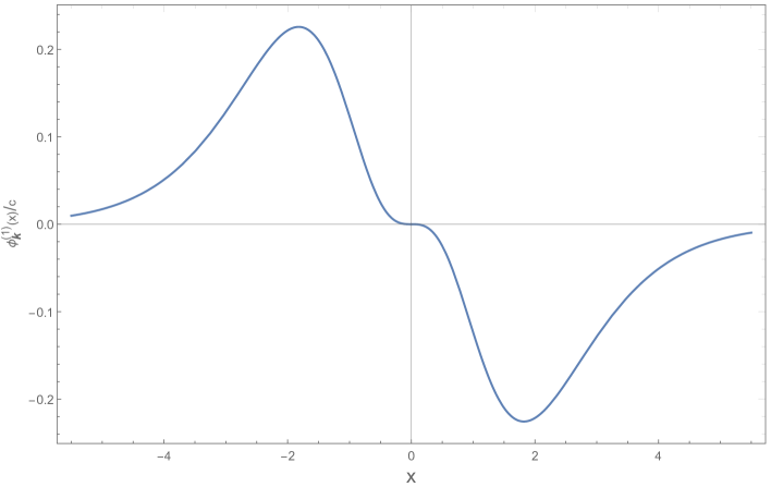
Figure 1: First order correction to the kink function due to Lorentz violation

3 Quantizing the Kinks

As we know, the trivial vacuum and kink are classical static solutions of a nonlinear relativistic field equation. In principle, they can be associated with quantum extended particle states. Therefore, we are now going to study the relevance of them to the corresponding quantum field theory. To do this, it may be thought that one needs either the Feynman path-integral or the canonical quantization methods. However, another simple method which is used in the literature is an approach through which one expands the energy corresponding to the static states via a semiclassical method. Then, using the classical solutions one can obtain a little information about the quantum behavior of the system. This semiclassical quantization technique has been firstly introduced for relativistic field theories, using an appropriate generalization of the WKB approximation in quantum mechanics by Dashen, Hasslacher and Neveu [38, 39]. For future use, here, we very briefly review this approach and some of its conclusions.

The energy of static states involves only the potential energy which can be expanded about a minimum as follows:

$$V[\phi]=V[\phi_{0}]+\int dx\frac{1}{2}\left[\zeta(x)\left(-\nabla^{2}+\left.\frac{d^{2}{\cal U}}{d\phi^{2}}\right|_{\phi_{0}(x)}\right)\zeta(x)\right]+\dots,$$ (14)

where $\zeta(x)=\phi(x)-\phi_{0}(x)$ and $\cal U$ is the interacting potential density along with the mass term. In fact, this is functional Taylor expansion of $V[\phi(x)]$ about the static solution $\phi_{0}(x)$. In Eq. (14), integration by part has been used and dots represent cubic and higher terms which can be treated by perturbation. This method can be used when the weak coupling approximation is established. The first term in Eq. (14) is related to classical contribution in energy. The second term is the leading order quantum correction which is similar to the harmonic oscillator with well-known quantum physics. We can find the normal modes by solving the following stability equation:

$$\left(-\nabla^{2}+\left.\frac{d^{2}{\cal U}}{d\phi^{2}}\right|_{\phi_{0}(x)}\right)\zeta_{n}(x)=\omega^{2}_{n}\zeta_{n}(x).$$ (15)

Now, one can construct the energy spectrum of a static state corrected by quantum fluctuations as follows:

$$E_{\{n_{i}\}}=V[\phi_{0}]+\sum_{i}\left(n_{i}+\frac{1}{2}\right)\omega_{i},$$ (16)

where $n_{i}$ is the excitation number of the $i$th normal mode. Using the Lagrangian Eq. (3), the Eq. (15) reduces to

$$\bigg{[}-\partial^{2}_{x}-1+3\phi_{0}^{2}(x)\bigg{]}\zeta_{n}(x)=\omega_{n}^{2}\zeta_{n}(x).$$ (17)

For the trivial vacuum $\phi_{0}=\phi_{\rm{tri.}}=\pm 1$, this equation has plane wave solutions $e^{\pm ikx}$ on which we can impose the Periodic Boundary Condition (PBC) in a box with length $L$. Therefore, $\omega_{n}^{2}=k_{n}^{2}+2$ with $k_{n}=2n\pi/L$, and the energy becomes

$$E_{\{n_{i}\}}^{\rm{trv.}}=\sum_{i=-\infty}^{+\infty}\left(n_{i}+\frac{1}{2}\right)\sqrt{k_{i}^{2}+2}.$$ (18)

For the $\phi_{0}=\phi_{\rm{k}}=\pm\tanh\left(\frac{x-x_{0}}{\sqrt{2}}\right)$, the Eq. (17) becomes

$$\bigg{[}-\partial^{2}_{x}-1+3\tanh^{2}\left(\frac{x}{\sqrt{2}}\right)\bigg{]}\zeta_{n}(x)=\omega_{n}^{2}\zeta_{n}(x),$$ (19)

where we choose $x_{0}=0$. The Eq. (19) has two bound state solutions (regardless of normalization factors)

$$\left\{\begin{array}[]{cc}\zeta_{0}(x)=\frac{1}{\cosh^{2}(x/\sqrt{2})}&\mbox{with}\quad\omega_{0}=0,\\ \zeta_{1}(x)=\frac{\sinh(x/\sqrt{2})}{\cosh^{2}(x/\sqrt{2})}&\qquad\mbox{with}\quad\omega_{1}=\sqrt{2/3},\end{array}\right.$$ (20)

followed by a continuum

$$\begin{array}[]{cc}&\zeta_{q}(x)=e^{iqx/\sqrt{2}}\left[3\tanh^{2}(x/\sqrt{2})-1-q^{2}-3iq\tanh(x/\sqrt{2})\right]\\ &\quad\mbox{with}\qquad\omega_{q}=\sqrt{2+q^{2}/2}.\end{array}$$ (21)

The zero mode is corresponding to the translational invariance of the potential. The asymptotic behavior of $\zeta_{q}(x)$ at $\pm\infty$ is $\exp[iqx/\sqrt{2}\pm\delta(q)/2]$ where $\delta(q)=-2\tan^{-1}\left(\frac{3q}{2-q^{2}}\right)$ is the phase shift of scattering states. Again, the PBC gives the allowed mumenta

$$q_{n}L/\sqrt{2}+\delta(q_{n})=2n\pi,$$ (22)

and the energy spectrum is

$$E_{\{n_{1},n_{q_{i}}\}}=\frac{2\sqrt{2}}{3}+\left(n_{1}+\frac{1}{2}\right)\sqrt{\frac{3}{2}}+\sum_{q_{i}}\left(n_{q_{i}}+\frac{1}{2}\right)\sqrt{2+\frac{q^{2}_{i}}{2}}\ .$$ (23)

For more details please see [37], for instance.

3.1 Excitations of the trivial vacuum

In this subsection we consider the quantization of the trivial solution in the LV theory. For this purpose, using Lagrangian (8) we expand the potential about one of its trivial vacuum. Similar to Eq. (14), the functional expansion up to the second order of $\zeta$ is written as follows:

$$V[\phi]=V[\phi_{\rm{tri.}}]+\int dx\left[\frac{1}{2}\zeta(x)\left(-(1+c)\partial^{2}_{x}+2\right)\zeta(x)\right]+\dots.$$ (24)

Accordingly, the eigenvalues in lowest-order quadratic terms are obtained from this equation

$$\left[-(1+c)\partial^{2}_{x}+2\right]\zeta_{n}(x)=\omega_{n}^{2}\zeta_{n}(x).$$ (25)

This equation has plane wave solutions $e^{\pm ikx}$ with $\omega_{n}^{2}=(1+c)k_{n}^{2}+2$. After imposing the PBC, we can write the energy as

$$E_{\{n_{i}\}}=\sum_{i}\left(n_{i}+\frac{1}{2}\right)\omega_{i}=\sum_{i=-\infty}^{+\infty}\left(n_{i}+\frac{1}{2}\right)\sqrt{(1+c)k_{i}^{2}+2},$$ (26)

where the classical energy $V[\phi_{\rm{tri.}}]$ is zero. We see from Eq. (26) (or Eq. (25)) that the Lorentz violation effect can be eliminated by the redefinition of $k_{n}$ (or spatial coordinate). Therefore, the vacuum solution does not receive any genuine correction due to the Lorentz violation in this case.

3.2 Excitations of kink

Now, we discuss the quantization of the kink. Similar to previous subsection, we can expand the potential $V[\phi]$ about the $\phi_{\rm{k}}$. Up to the second order of $\zeta$, one obtains the following expression for the potential:

$$\begin{array}[]{cc}&V[\phi]=V[\phi_{\rm{\rm{k}}}]+\int dx\frac{1}{2}\zeta(x)\bigg{[}-(1+c\phi_{k}^{2})\partial^{2}_{x}-3c(\partial_{x}\phi_{k})^{2}-3c(\partial_{x}\phi_{k}^{2})\partial_{x}\\ &\hskip 85.35826pt-4c\phi_{k}(\partial_{x}^{2}\phi_{k})-1+3\phi_{k}^{2}\bigg{]}\zeta(x).\end{array}$$ (27)

Therefore, the stability equation, read from Eq. (27), is

$$\bigg{[}-(1+c\phi_{k}^{2})\partial^{2}_{x}-3c(\partial_{x}\phi_{k})^{2}-3c(\partial_{x}\phi_{k}^{2})\partial_{x}-4c\phi_{k}(\partial_{x}^{2}\phi_{k})-1+3\phi_{k}^{2}\bigg{]}\zeta_{n}(x)=\omega_{n}^{2}\zeta_{n}(x)$$ (28)

The above equation can be solved via perturbation on LV parameter $c$. Hence, we expand our states $\zeta_{n}(x)$ and normal modes $\omega_{n}$ as

$$\zeta_{n}=\zeta_{n}^{(0)}+c\ {\zeta_{n}^{(1)}}+c^{2}{\zeta_{n}^{(2)}}+\dots,$$ (29)

$$\omega_{n}=\omega_{n}^{(0)}+c\ {\omega^{(1)}}+c^{2}{\omega_{n}^{(2)}}+\dots.$$ (30)

In the above equations $\zeta_{n}^{(0)}$ and $\omega_{n}^{(0)}$ are the leading order terms given by Eqs. (20) and (21). Accordingly, the order $c$ of Eq. (28) becomes

$$\left\{\partial_{x}^{2}+1+\left(\omega_{n}^{(0)}\right)^{2}-3\left[\phi_{\rm{k}}^{(0)}(x)\right]^{2}\right\}\zeta_{n}^{(1)}(x)+F_{n}(x)=0,$$ (31)

where

$$F_{n}(x)=\bigg{[}\left(\phi_{\rm{k}}^{(0)}\right)^{2}\partial_{x}^{2}+3\partial_{x}\left(\phi_{\rm{k}}^{(0)}\right)^{2}\partial_{x}+2\omega_{n}^{(0)}\omega_{n}^{(1)}$$

$$\hskip 48.36958pt-6\phi_{\rm{k}}^{(0)}\phi_{\rm{k}}^{(1)}+3\left(\partial_{x}\phi_{\rm{k}}^{(0)}\right)^{2}+4\phi_{\rm{k}}^{(0)}\partial_{x}^{2}\phi_{\rm{k}}^{(0)}\bigg{]}\zeta_{n}^{(0)}(x).$$ (32)

For the two bound states, the solutions of this equation are

$$\left\{\begin{array}[]{cc}\zeta^{(1)}_{0}(x)=\frac{1}{8}\text{sech}^{4}\left(\frac{x}{\sqrt{2}}\right)\left(2\sqrt{2}x\sinh\left(\sqrt{2}x\right)-9\cosh\left(\sqrt{2}x\right)+11\right)&\\ \hskip 179.25244pt\mbox{with}\quad\omega^{(1)}_{0}=0,\\ \zeta^{(1)}_{1}(x)=\frac{1}{20}\text{sech}\left(\frac{x}{\sqrt{2}}\right)\bigg{\{}5\sqrt{2}x\left(1-2\text{sech}^{2}\left(x/\sqrt{2}\right)\right)&\\ \hskip 28.45274pt+\tanh\left(\frac{x}{\sqrt{2}}\right)\left[-2\sqrt{2}x+4\log\left(e^{\sqrt{2}x}+1\right)+50\ \text{sech}^{2}\left(\frac{x}{\sqrt{2}}\right)-91/3\right]\bigg{\}}&\\ \hskip 202.01474pt\mbox{with}\quad\omega^{(1)}_{1}=\frac{1}{5\sqrt{6}}.&\\ \end{array}\right.$$ (33)

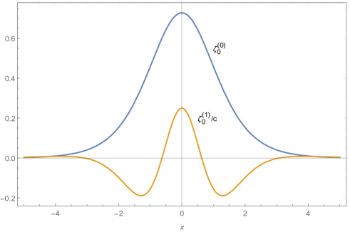
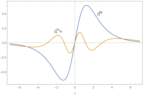
Figure 2: The zeroth and first order of two bound states.

Actually, $\omega_{0}$ does not receive any correction. To derive these solutions and their corresponding modes, we have taken the boundary condition at infinity into account. For comparison, we have plotted the zeroth and first order bound states in Fig. 2. For the continuum states, we can obtain corresponding frequencies by writing Eq. (31) at $x\to\pm\infty$

$$\left(2\partial_{x}^{2}+q^{2}\right)\zeta^{(1)}(x)+\left(q^{2}+3iq-2\right)\left(q^{2}-2\sqrt{2}\sqrt{q^{2}+4}\omega_{q}^{(1)}\right)e^{iqx/\sqrt{2}}=0.$$ (34)

Therefore, we get

$$\zeta^{(1)}_{q}(x)=\zeta^{(0)}_{q}(x)$$

$$\qquad+Q_{2}^{iq}\left[\tanh\left(x/\sqrt{2}\right)\right]\int_{1}^{\tanh\left(x/\sqrt{2}\right)}{{\cal F}_{q}(t)}P_{2}^{iq}(t)dt$$

$$\hskip 56.9055pt-iP_{2}^{iq}\left[\tanh\left(x/\sqrt{2}\right)\right]\int_{1}^{\tanh\left(x/\sqrt{2}\right)}{{\cal F}_{q}(t)}Q_{2}^{iq}(t)dt$$ (35)

$$\quad\mbox{with}\qquad\omega^{(1)}_{q}=\frac{q^{2}}{2\sqrt{2}\sqrt{q^{2}+4}}.$$ (36)

where,

$${{\cal F}_{q}(t)}=\frac{e^{iq\tanh^{-1}t}}{(3-iq)\left[P_{3}^{iq}(t)Q_{2}^{iq}(t)-P_{2}^{iq}(t)Q_{3}^{iq}(t)\right]}$$

$$\times[q^{4}+\left(-44q^{2}-105iqt+105t^{2}-68\right)t^{2}$$

$$+6\left(q^{2}+3iqt-3t^{2}+1\right)t\tanh^{-1}t+3i\left(3q^{2}+11\right)qt+4q^{2}+3]$$

and $P_{n}^{m}(x)$ and $Q_{n}^{m}(x)$ are the first and second kinds of the associated Legendre functions, respectively. From Eq. (34) we can see that the asymptotic form of the $\zeta^{(1)}_{q}(x)$ at infinity is $e^{\pm iqx/\sqrt{2}}$. Therefore we have

$$\zeta_{q}(x)\to e^{iqx/\sqrt{2}}\left[2-q^{2}-3iq+c\right]=\exp[iqx/\sqrt{2}\pm\delta(q)/2]\quad\mbox{at}\qquad x\to\pm\infty,$$ (38)

where the phase shift is

$$\delta(q)=-2\tan^{-1}\left(\frac{3q}{2+c-q^{2}}\right)=-2\tan^{-1}\left(\frac{3q}{2-q^{2}}\right)+\frac{6qc}{q^{4}+5q^{2}+4}+{\cal O}(c^{2}).$$ (39)

Here, the first term of the right hand side is the leading term of the phase shift (without Lorentz violation) and the second is the correction raised from Lorentz violation. Now, the correction to the energy spectrum becomes

$$E^{(1)}_{\{n_{1},n_{q_{i}}\}}=\frac{\sqrt{2}}{15}+\left(n_{1}+\frac{1}{2}\right)\frac{1}{5\sqrt{6}}+\sum_{q_{i}}\left(n_{q_{i}}+\frac{1}{2}\right)\frac{q_{i}^{2}}{2\sqrt{2}\sqrt{q_{i}^{2}+4}}$$ (40)

where $q_{i}$ are derived by substituting Eq. (39) in Eq. (22).

4 Summary

The Lorentz symmetry may be broken in high energies where the gravity must be quantized. Therefore, we need to check what causes the Lorentz violation in low energy theories. In this paper, we have studied the effects of an LV potential on the energy spectrum predicted for the $\phi^{4}$ scalar field theory in two space-time dimensions. We have considered an additional fundamental interaction $\frac{-c}{2}\phi^{2}(u.\partial\phi)^{2}$ that couples the derivative of a field to a constant vector describing LV. This is the lowest term which leads to nontrivial effects in the theory. The modifications of wave functions and the corresponding energy spectrum have been investigated for both trivial vacuum and kink. The trivial vacuum is not affected by the LV potential. However, up to the first order of the LV coefficient $c$, we have found the kink and its excitation modes (all bound and continuum states) are modified. One may expect such modifications because kink is a result of potential and this new LV term is also in the same order in $\phi$’s.

AcknowledgementThe authors would like to thank the Research Deputy of the University of Qom for financial support.

References

- Manton and Sutcliffe [2004] N. Manton and P. Sutcliffe, Topological solitons (Cambridge University Press, 2004).
- Belova and Kudryavtsev [1997] T. I. Belova and A. E. Kudryavtsev, Physics-Uspekhi 40, 359 (1997).
- Abrikosov [2004] A. Abrikosov, Reviews of modern physics 76, 975 (2004).
- Kleckner and Irvine [2013] D. Kleckner and W. T. Irvine, Nature physics 9, 253 (2013).
- Vilenkin and Shellard [2000] A. Vilenkin and E. P. S. Shellard, Cosmic strings and other topological defects (Cambridge University Press, 2000).
- t Hooft [1974] G. t’ Hooft, Nucl. Phys. B 79, 276 (1974).
- Schaefer [2002] T. Schäfer, Physical Review D 65, 094033 (2002).
- [8] M. Shifman and A. Yung,Reviews of Modern Physics, 79 1139 (2007).
- [9] A. Opfennann and G. Papadopoulos,Nuclear Physics B488 177 (1997).
- [10] J. F. Schonfeld, Nuclear Physics B161 125 (1979).
- [11] N. Graham and R. L. Jaffe., Nuclear Physics B544 432 (1999).
- Vachaspati [2006] T. Vachaspati, Kinks and domain walls: An introduction to classical and quantum solitons (Cambridge University Press, 2006).
- Cuevas-Maraver and Kevrekidis [2019] J. Cuevas-Maraver and P. G. Kevrekidis, in A Dynamical Perspective on the Model (Springer, 2019), pp. 137–162.
- Waterhouse [2019] A. Waterhouse, arXiv preprint arXiv:1908.09650 (2019).
- Kosteleckỳ and Potting [1995] V. A. Kosteleckỳ and R. Potting, Physical Review D 51, 3923 (1995).
- Carroll et al. [2001] S. M. Carroll, J. A. Harvey, V. A. Kosteleckỳ, C. D. Lane, and T. Okamoto, Physical Review Letters 87, 141601 (2001).
- Aghababaei and Haghighat [2017] S. Aghababaei and M. Haghighat, Physical Review D 96, 075017 (2017).
- Colladay and Kosteleckỳ [1998] D. Colladay and V. A. Kosteleckỳ, Physical Review D 58, 116002 (1998).
- [19] A. F. Santos and F. C. Khanna. Physics Letters B 762 283 (2016).
- [20] M. B. Cruz, E. R. Bezerra de Mello and A. Yu Petrov. Physical Review D 96 045019 (2017).
- [21] A. Mojavezi, R. Moazzemi and M. E. Zomorrodian. Nuclear Physics B941 145 (2019).
- [22] J. D. Tasson, Reports on Progress in Physics 77 062901 (2014).
- [23] Q. G. Bailey and V. A. Kostelecký, Physical Review D 70 076006 (2004).
- [24] R. Casana, M. M. Ferreira Jr and C. E. H. Santos, Physical Review D 78 025030 (2008).
- [25] Casana, Rodolfo, M. M. Ferreira Jr, A. R. Gomes, and P. R. D. Pinheiro. Physical Review D 80 125040 (2009).
- [26] H. Belich, M. M. Ferreira, and J. A. Helayel-Neto, The European Physical Journal C 38 511 (2005).
- [27] H. Belich, T. Costa-Soares, M.M. Ferreira Jr., J. A. Helay¨el-Neto, Eur. Phys. J. C 42, 127 (2005).
- Gopakumar et al. [2000] R. Gopakumar, S. Minwalla, and A. Strominger, Journal of High Energy Physics 2000, 020 (2000).
- Belich et al. [2005] H. Belich, T. Costa-Soares, M. FerreiraJr, and J. Helayël-Neto, The European Physical Journal C-Particles and Fields 41, 421 (2005).
- Seifert [2013] M. D. Seifert, in Proceedings of the Sixth Meeting on CPT and Lorentz Symmetry (World Scientific, 2013), pp. 212–215.
- Lubo [2005] M. Lubo, Physical Review D 71, 047701 (2005).
- Passos et al. [2018] E. Passos, C. Almeida, F. Brito, R. Menezes, J. Mota-Silva, and J. Santos, Annals of Physics 396, 351 (2018).
- Bazeia et al. [2010] D. Bazeia, M. Ferreira Jr, A. Gomes, and R. Menezes, Physica D: Nonlinear Phenomena 239, 942 (2010).
- Barreto et al. [2006] M. N. Barreto, D. Bazeia, and R. Menezes, Physical Review D 73, 065015 (2006).
- [35] S. M. Carroll and H. Tam, Physical Review D 78 044047 (2008).
- [36] M. Gomes, J. R. Nascimento, A. Yu Petrov, and A. J. Da Silva, Physical Review D 81 045018 (2010).
- Rajaraman [1982] R. Rajaraman, Solitons and instantons (North Holland, 1982).
- Dashen et al. [1974a] R. F. Dashen, B. Hasslacher, and A. Neveu, Physical Review D 10, 4114 (1974a).
- Dashen et al. [1974b] R. F. Dashen, B. Hasslacher, and A. Neveu, Physical Review D 10, 4130 (1974b).