GIST: Distributed Training for Large-Scale Graph Convolutional Networks

Abstract

The graph convolutional network (GCN) is a go-to solution for machine learning on graphs, but its training is notoriously difficult to scale both in terms of graph size and the number of model parameters. Although some work has explored training on large-scale graphs (e.g., GraphSAGE, ClusterGCN, etc.), we pioneer efficient training of large-scale GCN models (i.e., ultra-wide, overparameterized models) with the proposal of a novel, distributed training framework. Our proposed training methodology, called GIST, disjointly partitions the parameters of a GCN model into several, smaller sub-GCNs that are trained independently and in parallel. In addition to being compatible with all GCN architectures and existing sampling techniques for efficient GCN training, GIST $i)$ improves model performance, $ii)$ scales to training on arbitrarily large graphs, $iii)$ decreases wall-clock training time, and $iv)$ enables the training of markedly overparameterized GCN models. Remarkably, with GIST, we train an astonishgly-wide $32,\!768$-dimensional GraphSAGE model, which exceeds the capacity of a single GPU by a factor of $8\times$, to SOTA performance on the Amazon2M dataset.

1 Introduction

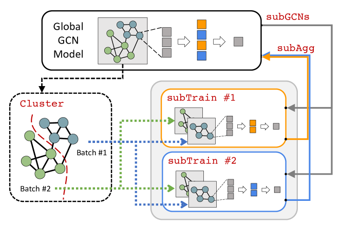
Figure 1: GIST pipeline: subGCNs divides the global GCN into sub-GCNs. Every sub-GCN is trained by subTrain using mini-batches (smaller sub-graphs) generated by Cluster. Sub-GCN parameters are intermittently aggregated through subAgg.

Since not all data can be represented in Euclidean space (Bronstein et al., 2017), many applications rely on graph-structured data. For example, social networks can be modeled as graphs by regarding each user as a node and friendship relations as edges (Lusher et al., 2013; Newman et al., 2002). Alternatively, in chemistry, molecules can be modeled as graphs, with nodes representing atoms and edges encoding chemical bonds (Balaban, 1985; Benkö et al., 2003).

To better understand graph-structured data, several (deep) learning techniques have been extended to the graph domain (Defferrard et al., 2016; Gori et al., 2005; Masci et al., 2015). Currently, the most popular one is the graph convolutional network (GCN) (Kipf & Welling, 2016), a multi-layer architecture that implements a generalization of the convolution operation to graphs. Although the GCN handles node- and graph-level classification, it is notoriously inefficient and unable to handle large-scale graphs (Chen et al., 2018b, a; Gao et al., 2018; Huang et al., 2018; You et al., 2020; Zeng et al., 2019).

To deal with these issues, node partitioning methodologies have been developed. These schemes can be roughly categorized into neighborhood sampling (Chen et al., 2018a; Hamilton et al., 2017; Zou et al., 2019) and graph partitioning (Chiang et al., 2019; Zeng et al., 2019) approaches. The goal is to partition a large graph into multiple smaller graphs that can be used as mini-batches for training the GCN. In this way, GCNs can handle larger graphs during training, expanding their potential into the realm of big data.

Although some papers perform large-scale experiments (Chiang et al., 2019; Zeng et al., 2019), the models (and data) used in GCN research remain small in the context of deep learning (Kipf & Welling, 2016; Veličković et al., 2017), where the current trend is towards incredibly large models and datasets (Brown et al., 2020; Conneau et al., 2019). Despite the widespread moral questioning of this trend (Hao, 2019; Peng & Sarazen, 2019; Sharir et al., 2020), the deep learning community continues to push the limits of scale, as overparameterized models are known to discover generalizable solutions (Nakkiran et al., 2019). Although deep GCN models suffer from oversmoothing (Kipf & Welling, 2016; Li et al., 2018), overparameterized GCN models can still be explored through larger hidden layers. As such, this work aims to provide a training framework that enables GCN experiments with wider models and larger datasets.

This paper. We propose a novel, distributed training methodology that can be used for any GCN architecture and is compatible with existing node sampling techniques. This methodology randomly partitions the hidden feature space in each layer, decomposing the global GCN model into multiple, narrow sub-GCNs of equal depth. Sub-GCNs are trained independently for several iterations in parallel prior to having their updates synchronized; see Figure 1. This process of randomly partitioning, independently training, and synchronizing sub-GCNs is repeated until convergence. We call this method graph independent subnetwork training (GIST). GIST can easily scale to arbitrarily large graphs and significantly reduces the wall-clock time of training large-scale GCNs, allowing larger models and datasets to be explored. We focus specifically on enabling the training of “ultra-wide” GCNs (i.e., GCN models with very large hidden layers), as deeper GCNs are prone to oversmoothing (Li et al., 2018). The contributions of this work are summarized below:

• We develop a novel, distributed training methodology for arbitrary GCN architectures, based on decomposing the model into independently-trained sub-GCNs. This methodology is compatible with existing techniques for neighborhood sampling and graph partitioning.

• We show that GIST can be used to train several GCN architectures to state-of-the-art performance with reduced training time in comparison to standard methodologies.

• We propose a novel Graph Independent Subnetwork Training Kernel (GIST-K) that allows a convergence rate to be derived for two-layer GCNs trained with GIST in the infinite width regime. Based on GIST-K, we provide theory that GIST converges linearly, up to an error neighborhood, using distributed gradient descent with local iterations. We show that the radius of the error neighborhood is controlled by the overparameterization parameter, as well as the number of workers in the distributed setting. Such findings reflect practical observations that are made in the experimental section.

• We use GIST to enable the training of markedly overparameterized GCN models. In particular, GIST is used to train a two-layer GraphSAGE model with a hidden dimension of 32,768 on the Amazon2M dataset. Such a model exceeds the capacity of a single GPU by $8\times$.

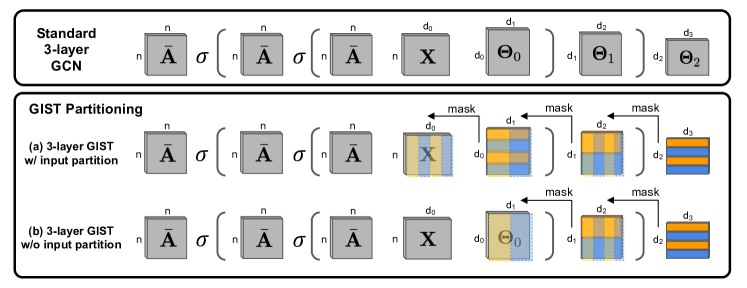
Figure 2: GCN partition into $m=2$ sub-GCNs. Orange and blue colors depict different feature partitions. Both hidden dimensions ($d_{1}$ and $d_{2}$) are partitioned. The output dimension ($d_{3}$) is not partitioned. Partitioning the input dimension ($d_{0}$) is optional. In this work, we do not partition $\mathbf{d}_{0}$ in GIST.

2 What is the GIST of this work?

Algorithm 1 GIST Algorithm

  Parameters: $T$ synchronization iterations, $m$ sub-GCNs $\zeta$ local iterations, $c$ clusters, $\mathcal{G}$ training graph.

  $\Psi_{\mathcal{G}}(\,\cdot\,;\boldsymbol{\Theta})$ $\leftarrow$ randomly initialize GCN

  $\{\mathcal{G}_{(j)}\}_{j=1}^{c}\leftarrow\text{{Cluster}}(\mathcal{G},c)$

  for $t=0,\dots,T-1$ do

     $\big{\{}\Psi_{\mathcal{G}}(\,\cdot\,;\boldsymbol{\Theta}^{(i)})\big{\}}_{i=1}^{m}\leftarrow\text{{subGCNs}}(\Psi_{\mathcal{G}}(\,\cdot\,;\boldsymbol{\Theta}),m)$

     Distribute each $\Psi_{\mathcal{G}}(\,\cdot\,;\boldsymbol{\Theta}^{(i)})$ to a different worker

     for $i=1,\dots,m$ do

        for $z=1,\dots,\zeta$ do

           $\Psi_{\mathcal{G}}(\,\cdot\,;\boldsymbol{\Theta}^{(i)})\leftarrow\text{{subTrain}}(\boldsymbol{\Theta}^{(i)},\{\mathcal{G}_{(j)}\}_{j=1}^{c})$

        end for

     end for

     $\Psi_{\mathcal{G}}(\,\cdot\,;\boldsymbol{\Theta})\leftarrow\text{{subAgg}}(\{\boldsymbol{\Theta}^{(i)}\}_{i=1}^{m})$

  end for

GCN Architecture. The GCN (Kipf & Welling, 2016) is arguably the most widely-used neural network architecture on graphs. Consider a graph $\mathcal{G}$ comprised of $n$ nodes with $d$-dimensional features $\mathbf{X}\in\mathbb{R}^{n\times d}$. The output $\mathbf{Y}\in\mathbb{R}^{n\times d^{\prime}}$ of a GCN can be expressed as $\mathbf{Y}=\Psi_{\mathcal{G}}(\mathbf{X};\boldsymbol{\Theta})$, where $\Psi_{\mathcal{G}}$ is an $L$-layered architecture with trainable parameters $\boldsymbol{\Theta}$. If we define $\mathbf{H}_{0}=\mathbf{X}$, we then have that $\mathbf{Y}=\Psi_{\mathcal{G}}(\mathbf{X};\boldsymbol{\Theta})=\mathbf{H}_{L}$, where an intermediate $\ell$-th layer of the GCN is given by

$$\mathbf{H}_{\ell+1}=\sigma(\bar{\mathbf{A}}\,\mathbf{H}_{\ell}\,\boldsymbol{\Theta}_{\ell}).$$ (1)

In (1), $\sigma$ is an elementwise activation function (e.g., ReLU), $\bar{\mathbf{A}}$ is the degree-normalized adjacency matrix of $\mathcal{G}$ with added self-loops, and the trainable parameters $\boldsymbol{\Theta}=\{\boldsymbol{\Theta}_{\ell}\}_{\ell=0}^{L-1}$ have dimensions $\boldsymbol{\Theta}_{\ell}\in\mathbb{R}^{d_{\ell}\times d_{\ell+1}}$ with $d_{0}=d$ and $d_{L}=d^{\prime}$. In Figure 2 (top), we illustrate nested GCN layers for $L=3$, but our methodology extends to arbitrary $L$. The activation function of the last layer is typically the identity or softmax transformation – we omit this in Figure 2 for simplicity.

GIST overview. We overview GIST in Algorithm 1 and present a schematic depiction in Figure 1. We partition our (randomly initialized) global GCN into $m$ smaller, disjoint sub-GCNs with the subGCNs function ($m=2$ in Figures 2 and 1) by sampling the feature space at each layer of the GCN; see Section 2.1. Each sub-GCN is assigned to a different worker (i.e., a different GPU) for $\zeta$ rounds of distributed, independent training through subTrain. Then, newly-learned sub-GCN parameters are aggregated (subAgg) into the global GCN model. This process repeats for $T$ iterations. Our graph domain is partitioned into $c$ sub-graphs through the Cluster function ($c=2$ in Figure 1). This operation is only relevant for large graphs ($n>50,\!000$), and we omit it ($c=1$) for smaller graphs that don’t require partitioning.

2.1 subGCNs: Constructing Sub-GCNs

GIST partitions a global GCN model into several narrower sub-GCNs of equal depth. Formally, consider an arbitrary layer $\ell$ and a random, disjoint partition of the feature set $[d_{\ell}]=\{1,2,\ldots,d_{\ell}\}$ into $m$ equally-sized blocks $\{\mathcal{D}^{(i)}_{\ell}\}_{i=1}^{m}$. Accordingly, we denote by $\boldsymbol{\Theta}^{(i)}_{\ell}=[\boldsymbol{\Theta}_{\ell}]_{\mathcal{D}^{(i)}_{\ell}\times\mathcal{D}^{(i)}_{\ell+1}}$ the matrix obtained by selecting from $\boldsymbol{\Theta}_{\ell}$ the rows and columns given by the $i$th blocks in the partitions of $[d_{\ell}]$ and $[d_{\ell+1}]$, respectively. With this notation in place, we can define $m$ different sub-GCNs $\mathbf{Y}^{(i)}=\Psi_{\mathcal{G}}(\mathbf{X}^{(i)};\boldsymbol{\Theta}^{(i)})=\mathbf{H}^{(i)}_{L}$ where $\mathbf{H}^{(i)}_{0}=\mathbf{X}_{[n]\times\mathcal{D}^{(i)}_{0}}$ and each layer is given by:

$$\mathbf{H}^{(i)}_{\ell+1}=\sigma(\bar{\mathbf{A}}\,\mathbf{H}^{(i)}_{\ell}\,\boldsymbol{\Theta}^{(i)}_{\ell}).$$ (2)

Sub-GCN partitioning is illustrated in Figure 2-(a), where $m=2$. Partitioning the input features is optional (i.e., (a) vs. (b) in Figure 2). We do not partition the input features within GIST so that sub-GCNs have identical input information (i.e., $\mathbf{X}^{(i)}=\mathbf{X}$ for all $i$); see Section 5.1. Similarly, we do not partition the output feature space to ensure that the sub-GCN output dimension coincides with that of the global model, thus avoiding any need to modify the loss function. This decomposition procedure (subGCNs in Algorithm 1) extends to arbitrary $L$.

2.2 subTrain: Independently Training Sub-GCNs

Assume $c=1$ so that the Cluster operation in Algorithm 1 is moot and $\{\mathcal{G}_{(j)}\}_{j=1}^{c}=\mathcal{G}$. Because $\mathbf{Y}^{(i)}$ and $\mathbf{Y}$ share the same dimension, sub-GCNs can be trained to minimize the same global loss function. One application of subTrain in Algorithm 1 corresponds to a single step of stochastic gradient descent (SGD). Inspired by local SGD (Lin et al., 2018), multiple, independent applications of subTrain are performed in parallel (i.e., on separate GPUs) for each sub-GCN prior to aggregating weight updates. The number of independent training iterations between synchronization rounds, referred to as local iterations, is denoted by $\zeta$, and the total amount of training is split across sub-GCNs. Ideally, the number sub-GCNs and local iterations should be increased as much as possible to minimize communication and training costs. In practice, however, such benefits may come at the cost of statistical inefficiency; see Section 5.1.

If $c>1$, subTrain first selects one of the $c$ subgraphs in $\{\mathcal{G}_{(j)}\}_{j=1}^{c}$ to use as a mini-batch for SGD. Alternatively, the union of several sub-graphs in $\{\mathcal{G}_{(j)}\}_{j=1}^{c}$ can be used as a mini-batch for training. Aside from using mini-batches for each SGD update instead of the full graph, the use of graph partitioning does not modify the training approach outlined above. Some form of node sampling must be adopted to make training tractable when the full graph is too large to fit into memory. However, both graph partitioning and layer sampling are compatible with GIST (see Sections 5.2 and 5.4). We adopt graph sampling in the main experiments due to the ease of implementation. The novelty of our work lies in the feature partitioning strategy of GIST for distributed training, which is an orthogonal technique to node sampling; see Section 2.3.

After each sub-GCN completes $\zeta$ training iterations, their updates are aggregated into the global model (i.e., subAgg function in Algorithm 1). Within subAgg, each worker replaces global parameter entries $\boldsymbol{\Theta}$ with its own parameters $\boldsymbol{\Theta}^{(i)}$, where no collisions occur due to the disjointness of sub-GCN partitions. Interestingly, not every parameter in the global GCN model is updated by subAgg. For example, focusing on $\boldsymbol{\Theta}_{1}$ in Figure 2-(a), one worker will be assigned $\boldsymbol{\Theta}^{(1)}_{1}$ (i.e., overlapping orange blocks), while the other worker will be assigned $\boldsymbol{\Theta}^{(2)}_{1}$ (i.e., overlapping blue blocks). The rest of $\boldsymbol{\Theta}_{1}$ is not considered within subAgg. Nonetheless, since sub-GCN partitions are randomly drawn in each cycle $t$, one expects all of $\boldsymbol{\Theta}$ to be updated multiple times if $T$ is sufficiently large.

2.3 What is the value of GIST?

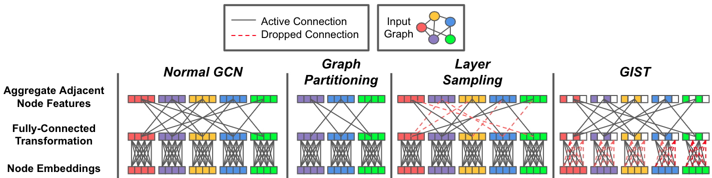
Figure 3: Illustrates the difference between GIST and node sampling techniques within the forward pass of a single GCN layer (excluding non-linear activation). While graph partitioning and layer sampling remove nodes from the forward pass (i.e., either completely or on a per-layer basis), GIST partitions node feature representations (and, in turn, model parameters) instead of the nodes themselves.

Architecture-Agnostic Distributed Training. GIST is a generic, distributed training methodology that can be used for any GCN architecture. We implement GIST for vanilla GCN, GraphSAGE, and GAT architectures, but GIST is not limited to these models; see Section 5.

Compatibility with Sampling Methods. GIST is NOT a replacement for graph or layer sampling. Rather, it is an efficient, distributed training technique that can be used in tandem with node partitioning. As depicted in Figure 3, GIST partitions node feature representations and model parameters between sub-GCNs, while graph partitioning and layer sampling sub-sample nodes within the graph.

Interestingly, we find that GIST’s feature and parameter partitioning strategy is compatible with node partitioning—the two approaches can be combined to yield further efficiency benefits. For example, GIST is combined with graph partitioning strategies in Section 5.2 and with layer sampling methodologies in Section 5.4.

Enabling Ultra-Wide GCN Training. GIST indirectly updates the global GCN through the training of smaller sub-GCNs, enabling models with hidden dimensions that exceed the capacity of a single GPU by a factor of $8\times$ to be trained. In this way, GIST allows markedly overparametrized (“ultra-wide”) GCN models to be trained on existing hardware. In Section 5.2, we leverage this capability to train a two-layer GCN model with a hidden dimension of 32,768 on Amazon2M.

We argue that overparameterization through width is more valuable than overparameterization through depth because deeper GCNs could suffer from oversmoothing (Li et al., 2018). As such, we do not explore depth-wise partitions of different GCN layers to each worker, but rather focus solely upon partitioning the hidden neurons within each layer. Such a partitioning strategy is suited to training wider networks.

Improved Model Complexity. Consider a single GCN layer, trained over $M$ machines with input and output dimension of $d_{i-1}$ and $d_{i}$, respectively. For one synchronization round, the communication complexity of GIST and standard distributed training is $\mathcal{O}(\frac{1}{M}d_{i}d_{i-1})$ and $\mathcal{O}(Md_{i}d_{i-1})$, respectively. GIST reduces communication by only communicating sub-GCN parameters. Existing node partitioning techniques cannot similarly reduce communication complexity because model parameters are never partitioned. Furthermore, the computational complexity of the forward pass for a GCN model trained with GIST and using standard methodology is $\mathcal{O}(\frac{1}{M}N^{2}d_{i}+\frac{1}{M^{2}}Nd_{i}d_{i-1})$ and $\mathcal{O}(N^{2}d_{i}+Nd_{i}d_{i-1})$, respectively, where $N$ is the number of nodes in the partition being processed. Node partitioning can reduce $N$ by a constant factor but is compatible with GIST.

3 Related Work

GCN training. In spite of their widespread success in several graph related tasks, GCNs often suffer from training inefficiencies (Gao et al., 2018; Huang et al., 2018). Consequently, the research community has focused on developing efficient and scalable algorithms for training GCNs (Chen et al., 2018b, a; Chiang et al., 2019; Hamilton et al., 2017; Zeng et al., 2019; Zou et al., 2019). The resulting approaches can be divided roughly into two areas: neighborhood sampling and graph partitioning. However, it is important to note that these two broad classes of solutions are not mutually exclusive, and reasonable combinations of the two approaches may be beneficial.

Neighborhood sampling methodologies aim to sub-select neighboring nodes at each layer of the GCN, thus limiting the number of node representations in the forward pass and mitigating the exponential expansion of the GCNs receptive field. VRGCN (Chen et al., 2018b) implements a variance reduction technique to reduce the sample size in each layer, which achieves good performance with smaller graphs. However, it requires to store all the intermediate node embeddings during training, leading to a memory complexity close to full-batch training. GraphSAGE (Hamilton et al., 2017) learns a set of aggregator functions to gather information from a node’s local neighborhood. It then concatenates the outputs of these aggregation functions with each node’s own representation at each step of the forward pass. FastGCN (Chen et al., 2018a) adopts a Monte Carlo approach to evaluate the GCN’s forward pass in practice, which computes each node’s hidden representation using a fixed-size, randomly-sampled set of nodes. LADIES (Zou et al., 2019) introduces a layer-conditional approach for node sampling, which encourages node connectivity between layers in contrast to FastGCN (Chen et al., 2018a).

Graph partitioning schemes aim to select densely-connected sub-graphs within the training graph, which can be used to form mini-batches during GCN training. Such sub-graph sampling reduces the memory footprint of GCN training, thus allowing larger models to be trained over graphs with many nodes. ClusterGCN (Chiang et al., 2019) produces a very large number of clusters from the global graph, then randomly samples a subset of these clusters and computes their union to form each sub-graph or mini-batch. Similarly, GraphSAINT (Zeng et al., 2019) randomly samples a sub-graph during each GCN forward pass. However, GraphSAINT also considers the bias created by unequal node sampling probabilities during sub-graph construction, and proposes normalization techniques to eliminate this bias.

As explained in Section 2, GIST also relies on graph partitioning techniques (Cluster) to handle large graphs. However, the feature sampling scheme at each layer (subGCNs) that leads to parallel and narrower sub-GCNs is a hitherto unexplored framework for efficient GCN training.

Distributed training. Distributed training is a heavily studied topic (Shi et al., 2020; Zhang et al., 2018). Our work focuses on synchronous and distributed training techniques (Lian et al., 2017; Yu et al., 2019; Zhang et al., 2015). Some examples of synchronous, distributed training approaches include data parallel training, parallel SGD (Agarwal & Duchi, 2011; Zinkevich et al., 2010), and local SGD (Lin et al., 2018; Stich, 2019). Our methodology holds similarities to model parallel training techniques, which have been heavily explored (Ben-Nun & Hoefler, 2019; Gholami et al., 2017; Günther et al., 2018; Kirby et al., 2020; Pauloski et al., 2020; Tavarageri et al., 2019; Zhu et al., 2020). More closely, our approach is inspired by independent subnetwork training (Yuan et al., 2019), explored for multi-layer perceptrons.

4 Theoretical Results

We draw upon analysis related to neural tangent kernels (NTK) (Jacot et al., 2018) to derive a convergence rate for two-layer GCNs using gradient descent—as formulated in (1) and further outlined in Appendix C.1—trained with GIST. Given the scaled Gram matrix of an infinite-dimensional NTK $\mathbf{H}^{\infty}$, we define the Graph Independent Subnetwork Training Kernel (GIST-K) as follows:

$$\mathbf{G}^{\infty}=\bar{\mathbf{A}}\mathbf{H}^{\infty}\bar{\mathbf{A}}.$$

Given the GIST-K, we adopt the following set of assumptions related to the underlying graph; see Appendix C.2 for more details.

Assumption 1.

Assume $\lambda_{\min}(\mathbf{\bar{A}})\neq 0$ and there exists $\epsilon\in(0,1)$ and $p\in\mathbb{Z}_{+}$ such that $(1-\epsilon)^{2}p\leq\mathbf{D}_{ii}\leq(1+\epsilon)^{2}p$ for all $i\in[n]=\{1,2,\dots,n\}$, where $\mathbf{D}$ is the degree matrix. Additionally, assume that $i)$ input node representations are bounded in norm and not parallel to any other node representation, $ii)$ output node representations are upper bounded, $iii)$ sub-GCN feature partitions are generated at each iteration from a categorical distribution with uniform mean $\frac{1}{m}$.

Given this set of assumptions, we derive the following result

Theorem 1.

Given assumption 1, if the number of hidden neurons within the two-layer GCN satisfies $d_{1}=\Omega\left(\frac{n^{3}\zeta^{2}T^{2}}{\delta^{2}\gamma(1-\gamma)^{2}\lambda_{0}^{4}}\left(n+\frac{d}{m^{2}}\|\bar{\mathbf{A}}^{2}\|_{1,1}\right)\right)$, then GIST with step-size $\eta=O\left(\frac{\lambda_{0}}{n^{2}\|\mathbf{A}^{2}\|_{1,1}}\right)$ converges with probability $1-\delta$ according to

$$\mathbb{E}_{[\mathcal{M}_{t-1}],\boldsymbol{\Theta}_{0},\mathbf{a}}\left[\left\|\mathbf{y}-\hat{\mathbf{y}}(t)\right\|_{2}^{2}\right]$$

$$\leq\left(\gamma+(1-\gamma)\left(1-\tfrac{\eta\lambda_{0}}{2}\right)^{\zeta}\right)^{t}\mathbb{E}_{\boldsymbol{\Theta}_{0},\mathbf{a}}\left[\|\mathbf{y}-\hat{\mathbf{y}}(0)\|_{2}^{2}\right]$$

$$\quad\quad\quad+O\left(\frac{(m-1)^{2}\zeta\|\bar{\mathbf{A}}^{2}\|_{1,1}nd}{\gamma m^{2}d_{1}}\right).$$

$m$	$d_{0}$	$d_{1}$	$d_{2}$	Cora	Citeseer	Pubmed	OGBN-Arxiv
Baseline				$81.52\pm 0.005$	$75.02\pm 0.018$	$75.90\pm 0.003$	$70.85\pm 0.089$
2	$\checkmark$	$\checkmark$	$\checkmark$	$80.00\pm 0.010$	$\mathbf{75.95}\pm 0.007$	$76.68\pm 0.011$	$65.65\pm 0.700$
	$\checkmark$	$\checkmark$		$78.30\pm 0.011$	$69.34\pm 0.018$	$75.78\pm 0.015$	$65.33\pm 0.347$
		$\checkmark$	$\checkmark$	$\textbf{80.82}\pm 0.010$	$75.82\pm 0.008$	$\textbf{78.02}\pm 0.007$	$\textbf{70.10}\pm 0.224$
4	$\checkmark$	$\checkmark$	$\checkmark$	$76.78\pm 0.017$	$70.66\pm 0.011$	$65.67\pm 0.044$	$54.21\pm 1.360$
	$\checkmark$	$\checkmark$		$66.56\pm 0.061$	$68.38\pm 0.018$	$68.44\pm 0.014$	$52.64\pm 1.988$
		$\checkmark$	$\checkmark$	$\mathbf{81.18}\pm 0.007$	$\mathbf{76.21}\pm 0.017$	$\mathbf{76.99}\pm 0.006$	$\textbf{68.69}\pm 0.579$
8	$\checkmark$	$\checkmark$	$\checkmark$	$48.32\pm 0.087$	$45.42\pm 0.092$	$54.29\pm 0.029$	$40.26\pm 1.960$
	$\checkmark$	$\checkmark$		$53.60\pm 0.020$	$54.68\pm 0.030$	$51.44\pm 0.002$	$26.84\pm 7.226$
		$\checkmark$	$\checkmark$	$\mathbf{79.58}\pm 0.006$	$\mathbf{75.39}\pm 0.016$	$\mathbf{76.99}\pm 0.006$	$\textbf{65.81}\pm 0.378$

Table 1: Test accuracy of GCN models trained on small-scale datasets with GIST. We selectively partition each feature dimension within the GCN model, indicated by a check mark. Partitioning on all hidden layers except the input layer leads to optimal performance.

A full proof of this result is deferred to Appendix C, but a sketch of the techniques used is as follows:

1. We define the GIST-K and show that it remains positive definite throughout training given our assumptions and sufficient overparameterization.

2. We show that local sub-GCN training converges linearly, given a positive definite GIST-K.

3. We analyze the change in training error when sub-GCNs are sampled (subGCNs), locally trained (subTrain), and aggregated (subAgg).

4. We establish a connection between local and aggregated weight perturbation, showing that network parameters are bounded by a small region centered around the initialization given sufficient overparameterization.

Discussion. Stated intuitively, the result in Theorem 1 shows that, given sufficient width, two-layer GCNs trained using GIST converge to approximately zero training error. The convergence rate is linear and on par with training the full, two-layer GCN model, up to an error neighborhood (i.e., without the feature partition utilized in GIST). Such theory shows that the feature partitioning strategy of GIST does not cause the model to diverge in training. Additionally, the theory suggests that wider GCN models and a larger number of sub-GCNs should be used to maximize the convergence rate of GIST and minimize the impact of the additive term within Theorem 1; though the affect of $m$ on the radius is less significant compared to $d_{1}$. Such findings reflect practical observations that are made within Section 5 and reveal that GIST is particularly-suited towards training extremely wide models that cannot be trained using a traditional, centralized approach on a single GPU.

5 Experiments

We use GIST to train different GCN architectures on six public, multi-node classification datasets; see Appendix A for details. In most cases, we compare the performance of models trained with GIST to that of models trained with standard methods (i.e., single GPU with node partitioning). Comparisons to models trained with other distributed methodologies are also provided in Appendix B. Experiments are divided into small and large scale regimes based upon graph size. The goal of GIST is to $i)$ train GCN models to state-of-the-art performance, $ii)$ minimize wall-clock training time, and $iii)$ enable training of very wide GCN models.

5.1 Small-Scale Experiments

In this section, we perform experiments over Cora, Citeseer, Pubmed, and OGBN-Arxiv datasets (Sen et al., 2008; Hu et al., 2020). For these small-scale datasets, we train a three-layer, 256-dimensional GCN model (Kipf & Welling, 2016) with GIST; see Appendix A.3 for further experimental settings. All reported metrics are averaged across five separate trials. Because these experiments run quickly, we use them to analyze the impact of different design and hyperparameter choices rather than attempting to improve runtime (i.e., speeding up such short experiments is futile).

Which layers should be partitioned? We investigate whether models trained with GIST are sensitive to the partitioning of features within certain layers. Although the output dimension $d_{3}$ is never partitioned, we selectively partition dimensions $d_{0}$, $d_{1}$, and $d_{2}$ to observe the impact on model performance; see Table 1. Partitioning input features ($d_{0}$) significantly degrades test accuracy because sub-GCNs observe only a portion of each node’s input features (i.e., this becomes more noticeable with larger $m$). However, other feature dimensions cause no performance deterioration when partitioned between sub-GCNs, leading us to partition all feature dimensions other than $d_{0}$ and $d_{L}$ within the final GIST methodology; see Figure 2-(b).

$L$	$m$	Reddit Dataset						Amazon2M Dataset
		GraphSAGE			GAT			GraphSAGE ($d_{i}=400$)			GraphSAGE ($d_{i}=4096$)
		F1	Time	Speedup	F1	Time	Speedup	F1	Time	Speedup	F1	Time	Speedup
2	-	96.09	105.78s	$1.00\times$	89.57	1.19hr	$1.00\times$	89.90	1.81hr	$1.00\times$	91.25	5.17hr	$1.00\times$
	2	96.40	70.29s	$1.50\times$	90.28	0.58hr	$2.05\times$	88.36	1.25hr	($1.45\times$)	90.70	1.70hr	$3.05\times$
	4	96.16	68.88s	$1.54\times$	90.02	0.31hr	$3.86\times$	86.33	1.11hr	($1.63\times$)	89.49	1.13hr	($4.57\times$)
	8	95.46	76.68s	$1.38\times$	89.01	0.18hr	$6.70\times$	84.73	1.13hr	($1.61\times$)	88.86	1.11hr	($4.65\times$)
3	-	96.32	118.37s	$1.00\times$	89.25	2.01hr	$1.00\times$	90.36	2.32hr	$1.00\times$	91.51	9.52hr	$1.00\times$
	2	96.36	80.46s	$1.47\times$	89.63	0.95hr	$2.11\times$	88.59	1.56hr	($1.49\times$)	91.12	2.12hr	$4.49\times$
	4	95.76	78.74s	$1.50\times$	88.82	0.48hr	$4.19\times$	86.46	1.37hr	($1.70\times$)	89.21	1.42hr	($6.72\times$)
	8	94.39	88.54s	($1.34\times$)	70.38	0.26hr	($7.67\times$)	84.76	1.37hr	($1.69\times$)	86.97	1.34hr	($7.12\times$)
4	-	96.32	120.74s	$1.00\times$	88.36	2.77hr	$1.00\times$	90.40	3.00hr	$1.00\times$	91.61	14.20hr	$1.00\times$
	2	96.01	91.75s	$1.32\times$	87.97	1.31hr	$2.11\times$	88.56	1.79hr	($1.68\times$)	91.02	2.77hr	$5.13\times$
	4	95.21	78.74s	($1.53\times$)	78.42	0.66hr	($4.21\times$)	87.53	1.58hr	($1.90\times$)	89.07	1.65hr	($8.58\times$)
	8	92.75	88.71s	($1.36\times$)	66.30	0.35hr	($7.90\times$)	85.32	1.56hr	($1.93\times$)	87.53	1.55hr	($9.13\times$)

Table 2: Performance of models trained with GIST on Reddit and Amazon2M. Parenthesis are placed around speedups achieved at a cost of $>$1 deterioration in F1 and $m=$“-” refers to the baseline. Models trained with GIST train more quickly and achieve comparable F1 score to those trained with standard methodology. The performance benefits of GIST become more pronounced for wider models.

How many Sub-GCNs to use? Using more sub-GCNs during GIST training typically improves runtime because sub-GCNs $i)$ become smaller, $ii)$ are each trained for fewer epochs, and $iii)$ are trained in parallel. We find that all models trained with GIST perform similarly for practical settings of $m$; see Table 1. One may continue increasing the number sub-GCNs used within GIST until all GPUs are occupied or model performance begins to decrease.

GIST Performance. Models trained with GIST often exceed the performance of models trained with standard, single-GPU methodology; see Table 1. Intuitively, we hypothesize that the random feature partitioning within GIST, which loosely resembles dropout (Srivastava et al., 2014), provides regularization benefits during training, but we leave an in-depth analysis of this property as future work.

5.2 Large-Scale Experiments

For large-scale experiments on Reddit and Amazon2M, the baseline model is trained on a single GPU and compared to models trained with GIST in terms of F1 score and training time. All large-scale graphs are partitioned into $15,\!000$ sub-graphs during training. Graph partitioning is mandatory because the training graphs are too large to fit into memory. One could instead use layer sampling to make training tractable (see Section 5.4), but we adopt graph partitioning in most experiments because the implementation is simple and performs well.

Reddit Dataset. We perform tests with $256$-dimensional GraphSAGE (Hamilton et al., 2017) and GAT (Veličković et al., 2017) models with two to four layers on Reddit; see Appendix A.4 for more details. As shown in Table 2, utilizing GIST significantly accelerates GCN training (i.e., a $1.32\times$ to $7.90\times$ speedup). GIST performs best in terms of F1 score with $m=2$ sub-GCNs (i.e., $m=4$ yields further speedups but F1 score decreases). Interestingly, the speedup provided by GIST is more significant for models and datasets with larger compute requirements. For example, experiments with the GAT architecture, which is more computationally expensive than GraphSAGE, achieve a near-linear speedup with respect to $m$.

Amazon2M Dataset. Experiments are performed with two, three, and four-layer GraphSAGE models (Hamilton et al., 2017) with hidden dimensions of $400$ and $4096$ (we refer to these models as “narrow” and “wide”, respectively). We compare the performance (i.e., F1 score and wall-clock training time) of GCN models trained with standard, single-GPU methodology to that of models trained with GIST; see Table 2. Narrow models trained with GIST have a lower F1 score in comparison to the baseline, but training time is significantly reduced. For wider models, GIST provides a more significant speedup (i.e., up to $7.12\times$) and tends to achieve comparable F1 score in comparison to the baseline, revealing that GIST works best with wider models.

Within Table 2, models trained with GIST tend to achieve a wall-clock speedup at the cost of a lower F1 score (i.e., observe the speedups marked with parenthesis in Table 2). When training time is analyzed with respect to a fixed F1 score, we observe that the baseline takes significantly longer than GIST to achieve a fixed F1 score. For example, when $L=2$, a wide GCN trained with GIST ($m=8$) reaches an F1 score of 88.86 in $\sim$4,000 seconds, while models trained with standard methodology take $\sim$10,000 seconds to achieve a comparable F1 score. As such, GIST significantly accelerates training relative to model performance.

$L$	$m$	F1 Score (Time)
		$d_{i}=400$	$d_{i}=4096$	$d_{i}=8192$	$d_{i}=16384$	$d_{i}=32768$
2	-	89.38 (1.81hr)	90.58 (5.17hr)	OOM	OOM	OOM
	2	87.48 (1.25hr)	90.09 (1.70hr)	90.87 (2.76hr)	90.94 (9.31hr)	90.91 (32.31hr)
	4	84.82 (1.11hr)	88.79 (1.13hr)	89.76 (1.49hr)	90.10 (2.24hr)	90.17 (5.16hr)
	8	82.56 (1.13hr)	87.16 (1.11hr)	88.31 (1.20hr)	88.89 (1.39hr)	89.46 (1.76hr)
3	-	89.73 (2.32hr)	90.99 (9.52hr)	OOM	OOM	OOM
	2	87.79 (1.56hr)	90.40 (2.12hr)	90.91 (4.87hr)	91.05 (17.7hr)	OOM
	4	85.30 (1.37hr)	88.51 (1.42hr)	89.75 (2.07hr)	90.15 (3.44hr)	OOM
	8	82.84 (1.37hr)	86.12 (1.34hr)	88.38 (1.37hr)	88.67 (1.88hr)	88.66 (2.56hr)
4	-	89.77 (3.00hr)	91.02 (14.20hr)	OOM	OOM	OOM
	2	87.75 (1.79hr)	90.36 (2.77hr)	91.08 (6.92hr)	91.09 (26.44hr)	OOM
	4	85.32 (1.58hr)	88.50 (1.65hr)	89.76 (2.36hr)	90.05 (4.93hr)	OOM
	8	83.45 (1.56hr)	86.60 (1.55hr)	88.13 (1.61hr)	88.44 (2.30hr)	OOM

Table 3: Performance of GraphSAGE models of different widths trained with GIST on Amazon2M. $m=$“-” refers to the baseline and “OOM” marks experiments that cause out-of-memory errors. GIST enables training of higher-performing, ultra-wide models.

5.3 Training Ultra-Wide GCNs

We use GIST to train GraphSAGE models with widths as high as 32K (i.e., $\boldsymbol{8\times}$ beyond the capacity of a single GPU); see Table 3 for results and Appendix A.5 for more details. Considering $L=2$, the best-performing, single-GPU GraphSAGE model ($d_{i}=4096$) achieves an F1 score of $90.58$ in $5.2$ hours. With GIST ($m=2$), we achieve a higher F1 score of $90.87$ in $2.8$ hours (i.e., a $1.86\times$ speedup) using $d_{i}=8192$, which is beyond single GPU capacity. Similar patterns are observed for deeper models. Furthermore, we find that utilizing larger hidden dimensions yields further performance improvements, revealing the utility of wide, overparameterized GCN models. GIST, due to its feature partitioning strategy, is unique in its ability to train models of such scale to state-of-the-art performance.

5.4 GIST with Layer Sampling

As previously mentioned, some node partitioning approach must be adopted to avoid memory overflow when the underlying training graph is large. Although graph partitioning is used within most experiments (see Section 5.2), GIST is also compatible with other node partitioning strategies. To demonstrate this, we perform training on Reddit using GIST combined with a recent layer sampling approach (Zou et al., 2019) (i.e., instead of graph partitioning); see Appendix A.6 for more details.

As shown in Table 4, combining GIST with layer sampling enables training on large-scale graphs, and the observed speedup actually exceeds that of GIST with graph partitioning. For example, GIST with layer sampling yields a $1.83\times$ speedup when $L=2$ and $m=2$, in comparison to a $1.50\times$ speedup when graph partitioning is used within GIST (see Table 2). As the number of sub-GCNs is increased beyond $m=2$, GIST with layer sampling continues to achieve improvements in wall-clock training time (e.g., speedup increases from $1.83\times$ to $2.90\times$ from $m=2$ to $m=4$ for $L=2$) without significant deterioration to model performance. Thus, although node partitioning is needed to enable training on large-scale graphs, the feature partitioning strategy of GIST is compatible with numerous sampling strategies (i.e., not just graph sampling).

$L$	# Sub-GCNs	GIST + LADIES
		F1 Score	Time	Speedup
2	Baseline	89.73	3359.91s	$1.00\times$
	2	89.29	1834.59s	$1.83\times$
	4	88.42	1158.51s	$2.90\times$
3	Baseline	89.57	4803.88s	$1.00\times$
	2	86.52	2635.18s	$1.82\times$
	4	86.72	1605.32s	$3.00\times$

Table 4: Performance of GCN models trained with a combination of GIST and LADIES (Zou et al., 2019) on Reddit. Here, the baseline represents models trained with LADIES in a standard, single-GPU manner. Combining GIST with layer sampling leads to further improvements in wall-clock training time without deteriorating the F1 score.

6 Conclusion

We present GIST, a distributed training approach for GCNs that enables the exploration of larger models and datasets. GIST is compatible with existing sampling approaches and leverages a feature-wise partition of model parameters to construct smaller sub-GCNs that are trained independently and in parallel. We have shown that GIST achieves remarkable speed-ups over large graph datasets and even enables the training of GCN models of unprecedented size. We hope GIST can empower the exploration of larger, more powerful GCN architectures within the graph community.

Appendix A Experimental Details

A.1 Datasets

The details of the datasets utilized within GIST experiments in Section 5 are provided in Table 5. Cora, Citeseer, PubMed and OGBN-Arxiv are considered “small-scale” datasets and are utilized within experiments in Section 5.1. Reddit and Amazon2M are considered “large-scale” datasets and are utilized within experiments in Section 5.2.

Dataset	$n$	# Edges	# Labels	$d$
Cora	2,708	5,429	7	1,433
CiteSeer	3,312	4,723	6	3,703
Pubmed	19,717	44,338	3	500
OGBN-Arxiv	169,343	1.2M	40	128
Reddit	232,965	11.6 M	41	602
Amazon2M	2.5 M	61.8 M	47	100

Table 5: Details of relevant datasets.

A.2 Implementation Details

We provide an implementation of GIST in PyTorch (Paszke et al., 2019) using the NCCL distributed communication package for training GCN (Kipf & Welling, 2016), GraphSAGE (Hamilton et al., 2017) and GAT (Veličković et al., 2017) architectures. Our implementation is centralized, meaning that a single process serves as a central parameter server. From this central process, the weights of the global model are maintained and partitioned to different worker processes (including itself) for independent training. Experiments are conducted with $8$ NVIDIA Tesla V100-PCIE-32G GPUs, a 56-core Intel(R) Xeon(R) CPU E5-2680 v4 @ 2.40GHz, and 256 GB of RAM.

A.3 Small-Scale Experiments

Small-scale experiments in Section 5.1 are performed using Cora, Citeseer, Pubmed, and OGBN-Arxiv datasets (Sen et al., 2008; Hu et al., 2020). GIST experiments are performed with two, four, and eight sub-GCNs in all cases. We find that the performance of models trained with GIST is relatively robust to the number of local iterations $\zeta$, but test accuracy decreases slightly as $\zeta$ increases; see Figure 5. Based on the results in Figure 5, we adopt $\zeta=20$ for Cora, Citeseer, and Pubmed, as well as $\zeta=100$ for OGBN-Arxiv.

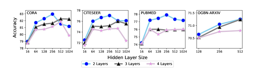
Figure 4: Test accuracy for different sizes (i.e., varying depth and width) of GCN models trained with standard, single-GPU methodology on small-scale datasets. We adopt three-layer, 256-dimensional GCN models as our baseline architecture.

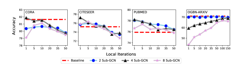
Figure 5: Test accuracy of GCN models trained on small-scale datasets with GIST using different numbers of local iterations and sub-GCNs. Models trained with GIST are surprisingly robust to the number of local iterations used during training, no matter the number of sub-GCNs.

Experiments are run for 400 epochs with a step learning rate schedule (i.e., $10\times$ decay at 50% and 75% of total epochs). A vanilla GCN model, as described in (Kipf & Welling, 2016), is used. The model is trained in a full-batch manner using the Adam optimizer (Kingma & Ba, 2014). No node sampling techniques are employed because the graph is small enough to fit into memory. All reported results are averaged across five trials with different random seeds. For all models, $d_{0}$ and $d_{L}$ are respectively given by the number of features and output classes in the dataset. The size of all hidden layers is the same, but may vary across experiments.

We first train baseline GCN models of different depths and hidden dimensions using a single GPU to determine the best model depth and hidden dimension to be used in small-scale experiments. The results are shown in Figure 4. Deeper models do not yield performance improvements for small-scale datasets, but test accuracy improves as the model becomes wider. Based upon the results in Figure 4, we adopt a three-layer GCN with a hidden dimension of $d_{1}\!=\!d_{2}\!=\!256$ as the underlying model used in small-scale experiments. Though two-layer models seem to perform best, we use a three-layer model within Section 5.1 to enable more flexibility in examining the partitioning strategy of GIST.

A.4 Large-Scale Experiments

Reddit Dataset. For experiments on Reddit, we train 256-dimensional GraphSAGE and GAT models using both GIST and standard, single-GPU methodology. During training, the graph is partitioned into $15,\!000$ sub-graphs. Training would be impossible without such partitioning because the graph is too large to fit into memory. The setting for the number of sub-graphs is the optimal setting proposed in previous work (Chiang et al., 2019). Models trained using GIST and standard, single-GPU methodologies are compared in terms of F1 score and training time.

All tests are run for $80$ epochs with no weight decay, using the Adam optimizer (Kingma & Ba, 2014). We find that $\zeta=500$ achieves consistently high performance for models trained with GIST on Reddit. We adopt a batch size of 10 sub-graphs throughout the training process, which is the optimal setting proposed in previous work (Chiang et al., 2019).

Amazon2M Dataset. For experiments on Amazon2M, we train two to four layer GraphSAGE models with hidden dimensions of $400$ and $4096$ using both GIST and standard, single-GPU methodology. We follow the experimental settings of (Chiang et al., 2019). The training graph is partitioned into $15,\!000$ sub-graphs and a batch size of $10$ sub-graphs is used. We find that using $\zeta=5000$ performs consistently well. Models are trained for $400$ total epochs with the Adam optimizer (Kingma & Ba, 2014) and no weight decay.

A.5 Training Ultra-Wide GCNs

All settings for ultra-wide GCN experiments in Section 5.3 are adopted from the experimental settings of Section 5.2; see Appendix A.4 for further details. For $d_{i}>4096$ evaluation must be performed on graph partitions (not the full graph) to avoid memory overflow. As such, the graph is partitioned into $5,\!000$ sub-graphs during testing and F1 score is measured over each partition and averaged. All experiments are performed using a GraphSAGE model, and the hidden dimension of the underlying model is changed between different experiments.

A.6 GIST with Layer Sampling

Experiments in Section 5.4 adopt the same experimental settings as Section 5.2 for the Reddit dataset; see Appendix A.4 for further details. Within these experiments, we combine GIST with LADIES (Zou et al., 2019), a recent layer sampling approach for efficient GCN training. LADIES is used instead of graph partitioning. Any node sampling approach can be adopted—some sampling approach is just needed to avoid memory overflow.

We train 256-dimensional GCN models with either two or three layers. We utilize a vanilla GCN model within this section (as opposed to GraphSAGE or GAT) to simplify the implementation of GIST with LADIES, which creates a disparity in F1 score between the results in Section 5.4 and Section 5.2. Experiments in Section 5.4 compare the performance of the same models trained either with GIST or using standard, single-GPU methodology. In this case, the single-GPU model is just a GCN trained with LADIES.

Appendix B Comparisons to Other Distributed Training Methodologies

Although GIST has been shown to provide benefits in terms of GCN performance and training efficiency in comparison to standard, single-GPU training, other choices for the distributed training of GCNs exist. Within this section, we compare GIST to other natural choices for distributed training, revealing that GCN models trained with GIST achieve favorable performance in comparison to those trained with other common distributed training techniques.

# Machines	Method	F1 Score	Training Time
2	Local SGD	96.37	137.17s
	GIST	96.40	108.67s
4	Local SGD	95.00	127.63s
	GIST	96.16	116.56s
8	Local SGD	93.40	129.58s
	GIST	95.46	123.83s

Table 6: Performance of GraphSAGE models trained using local SGD and GIST on Reddit. We adopt settings described in Section 5.2, but use 100 local iterations for both GIST and local SGD. Models trained with GIST outperform those trained with local SGD in terms of test F1 score and wall-clock training time in all cases.

B.1 Local SGD

A simple version of local SGD (Lin et al., 2018) can be implemented for distributed training of GCNs by training the full model on each separate worker for a certain number of local iterations and intermittently averaging local updates. In comparison to such a methodology, GIST has better computational and communication efficiency because $i)$ it communicates only a small fraction of model parameters to each machine and $ii)$ locally training narrow sub-GCNs is faster than locally training the full model. We perform a direct comparison between local SGD and GIST on the Reddit dataset using a two-layer, 256-dimensional GraphSAGE model; see Table 6. As can be seen, GCN models trained with GIST have lower wall-clock training time and achieve better performance than those trained with local SGD in all cases.

# Machines	Method	F1 Score	Inference Time
2	Ensemble	96.31	3.59s
	GIST	96.40	1.81s
4	Ensemble	96.10	6.38s
	GIST	96.16	1.81s
8	Ensemble	95.28	11.95s
	GIST	95.46	1.81s

Table 7: Performance of GraphSAGE models trained both with GIST and as ensembles of shallow sub-GCNs on Reddit. Models trained with GIST perform better and do not suffer from increased inference time as the number of sub-GCNs is increased.

B.2 Sub-GCN Ensembles

As previously mentioned, increasing the number of local iterations (i.e., $\zeta$ in Algorithm 1) decreases communication requirements given a fixed amount of training. When taken to the extreme (i.e., $\zeta\rightarrow\infty$), one could minimize communication requirements by never aggregating sub-GCN parameters, thus forming an ensemble of independently-trained sub-GCNs. We compare GIST to such a methodology in Table 7 using a two-layer, 256-dimensional GraphSAGE model on the Reddit dataset. Though training ensembles of sub-GCNs minimizes communication, Table 7 reveals that $i)$ models trained with GIST achieve better performance and $ii)$ inference time for sub-GCN ensembles becomes burdensome as the number of sub-GCNs is increased.

Appendix C Theoretical Results

C.1 Formulation of GIST for One-Hidden-Layer GCNs

In our analysis, we consider a GCN with one hidden-layer and a ReLU activation. We assume that the GCN outputs a scalar value $\tilde{y}_{i}$ for each node in the graph. Denoting $\tilde{\mathbf{y}}=[\tilde{y}_{1},\dots,\tilde{y}_{n}]$, we can write the output of the GCN as

$$\tilde{\mathbf{y}}=\frac{1}{\sqrt{d_{1}}}\bar{\mathbf{A}}\sigma(\bar{\mathbf{A}}\mathbf{X}\boldsymbol{\Theta})\mathbf{a}$$

where $\boldsymbol{\Theta}=[\boldsymbol{\theta}_{1},\dots,\boldsymbol{\theta}_{d_{1}}]\in\mathbb{R}^{n\times d_{1}}$ is the weights within the GCN’s first layer and $\mathbf{a}=[a_{1},\dots,a_{d_{1}}]\in\mathbb{R}^{d_{1}}$ is the weights within the GCN’s second layer. To simplify the analysis, we denote $\hat{\mathbf{X}}=\bar{\mathbf{A}}\mathbf{X}=[\mathbf{\hat{x}}_{1},\dots\mathbf{\hat{x}}_{n}]$. Then, we have $\hat{\mathbf{x}}_{i}=\sum_{i^{\prime}=1}^{n}\bar{\mathbf{A}}_{ii^{\prime}}\mathbf{x}_{i^{\prime}}$ and the output of each node within the graph can be written as

$$\tilde{y}_{i}=\frac{1}{\sqrt{d_{1}}}\sum_{i^{\prime}=1}^{n}\sum_{r=1}^{d_{1}}\bar{\mathbf{A}}_{ii^{\prime}}a_{r}\sigma(\left\langle\mathbf{\hat{x}}_{i^{\prime}},\boldsymbol{\theta}_{r}\right\rangle)$$

As in previous convergence analysis for training neural networks, we assume that second-layer weights $\mathbf{a}$ are fixed and only the first layer weights $\boldsymbol{\Theta}$ are trainable. Following the GIST feature partitioning strategy, we only partition the hidden layer. Specifically, in global iteration $t$, sub-GCNs are constructed by sampling a set of masks $\mathcal{M}_{t}\in\mathbb{R}^{m\times d_{1}}$. We denote the $j$th column of $\mathcal{M}_{t}$ as $\mathcal{M}^{(j)}_{t}\in\mathbb{R}^{m}$, the $r$th row of $\mathcal{M}_{t}$ as $\mathcal{M}_{t,r}\in\mathbb{R}^{d_{1}}$, and the entry in the $r$th row and $j$th column as $\mathcal{M}_{t,r}^{(j)}$. Each $\mathcal{M}^{(j)}_{t,r}$ is a binary values: $\mathcal{M}^{(j)}_{t,r}=1$ if neuron $r$ is active in sub-GCN $j$, and $\mathcal{M}^{(j)}_{t,r}=0$ otherwise. Using this mask notation, the output for node $i$ within sub-GCN $j$ can be written as

$$\hat{y}_{i}^{(j)}(t,k)=f_{\mathcal{M}_{t}^{(j)}}(\boldsymbol{\Theta}_{t,k}^{(j)},\mathbf{X})_{i}=\frac{1}{\sqrt{d_{1}}}\sum_{i^{\prime}=1}^{n}\sum_{r=1}^{d_{1}}\bar{\mathbf{A}}_{ii^{\prime}}\mathcal{M}_{t,r}^{(j)}a_{r}\sigma\left(\left\langle\hat{\mathbf{x}_{i^{\prime}}},\boldsymbol{\theta}_{t,k,r}^{(j)}\right\rangle\right)$$

$t$ and $k$ denote the current global and local iterations, respectively. We assume that each $\mathcal{M}_{t,r}$ is sampled from a one-hot categorical distribution. We formally define the random variables $\mathcal{M}_{t,r}^{(j)}$ as follows: Let each $\hat{m}_{t,r}$ be a uniform random variable on the index set $[m]=\{1,\dots,m\}$, i.e., $\mathcal{P}(\hat{m}_{t,r}=j)=\frac{1}{m}$ for $j\in[m]$. Then, we define each mask entry as $\mathcal{M}_{t,r}^{(j)}=\mathbb{I}\{\hat{m}_{k,r}=j\}$. Masks sampled in such a fashion have the following properties

• $\mathcal{P}(\mathcal{M}_{t,r}^{(j)}=1)=\frac{1}{m}$

• $\mathcal{P}(\mathcal{M}_{t,r}^{(j)}=0)=1-\frac{1}{m}$

• $\sum_{j=1}^{m}\mathcal{M}_{t,r}^{(j)}=1$

• $\mathcal{M}_{t,r}^{(j)}\mathcal{M}_{t,r}^{(j^{\prime})}=0$ if $j^{\prime}\neq j$.

Here, the first and second properties guarantee that the expected number of neurons active in each sub-GCN is equal. The third and fourth properties guarantee that each neuron is active in one and only one sub-GCN. Within this setup, we consider the GIST training procedure, described as

$$\boldsymbol{\theta}_{t,0,r}^{(j)} =\boldsymbol{\theta}_{t,r}$$ (3)

$$\boldsymbol{\theta}_{t,k+1,r}^{(j)} =\boldsymbol{\theta}_{t,k,r}^{(j)}-\eta\frac{\partial L(\boldsymbol{\Theta}_{t,k}^{(j)})}{\partial\boldsymbol{\theta}_{r}}$$

$$\boldsymbol{\theta}_{t+1,r} =\boldsymbol{\theta}_{t,r}+\sum_{j=1}^{m}\left(\boldsymbol{\theta}_{t,\zeta,r}^{(j)}-\boldsymbol{\theta}_{t,0,r}^{(j)}\right)$$

Within this formulation, $\zeta$ represents the total number of local iterations performed for each sub-GCN, while $L(\boldsymbol{\Theta}_{t,k}^{(j)})$ is the loss on the $j$th sub-GCN during the $t$th global and $k$th local iteration. We can express $L(\boldsymbol{\Theta}_{t,k}^{(j)})$ as

$$L\left(\boldsymbol{\Theta}_{t,k}^{(j)}\right)=\left\|\mathbf{y}-\hat{\mathbf{y}}^{(j)}(t,k)\right\|_{2}^{2}=\left\|\mathbf{y}-f_{\mathcal{M}_{t}^{(j)}}(\boldsymbol{\Theta}_{t,k}^{(j)},\mathbf{X})\right\|_{2}^{2}$$

and the gradient has the form

$$\frac{\partial L(\boldsymbol{\Theta}_{t,k}^{(j)})}{\partial\boldsymbol{\theta}_{r}}=\frac{1}{\sqrt{d_{1}}}\sum_{i=1}^{n}\sum_{i^{\prime}=1}^{n}\left(\hat{y}_{i}^{(j)}(t,k)-y_{i}\right)\bar{\mathbf{A}}_{ii^{\prime}}\mathcal{M}_{t,r}^{(j)}a_{r}\mathbf{\hat{x}}_{i^{\prime}}\mathbb{I}\left\{\left\langle\boldsymbol{\theta}_{t,k,r}^{(j)},\mathbf{\hat{x}}_{i^{\prime}}\right\rangle\geq 0\right\}$$

C.2 Properties of the Transformed Input

The GCN (Kipf & Welling, 2016) uses a first-degree Chebyshev polynomial to approximate a spectral convolution on the graph, which results in an aggregation matrix of the form

$$\bar{\mathbf{A}}=\mathbf{I}+\mathbf{D}^{-\frac{1}{2}}\mathbf{A}\mathbf{D}^{-\frac{1}{2}}$$ (4)

where $\mathbf{A}$ is the adjacency matrix and $\mathbf{D}$ is the degree matrix with $\mathbf{D}_{ii}=\sum_{j=1}^{n}\mathbf{A}_{ij}$. In practice, the re-normalization trick is applied to control the magnitude of the largest eigenvalue of $\bar{\mathbf{A}}$. Here, however, we keep the original formulation of (4) to facilitate our analysis, and our assumption on the depth of the GCN does not lead to numerical instability even if $\lambda_{\max}(\bar{\mathbf{A}})>1$. It is a well-known result that $2=\lambda_{\max}(\bar{\mathbf{A})}\geq\lambda_{\min}(\bar{\mathbf{A}})\geq 0$. In particular, the lower bound on the minimum eigenvalue is obtained by considering

$$\mathbf{v}^{\top}\bar{\mathbf{A}}\mathbf{v}=\sum_{i=1}^{n}v_{i}^{2}+\sum_{(i,j)\in E}\frac{v_{i}v_{j}}{\sqrt{\mathbf{D}_{ii}\mathbf{D}_{jj}}}=\sum_{(i,j)\in E}\left(\frac{v_{i}}{\sqrt{\mathbf{D}_{ii}}}+\frac{v_{j}}{\sqrt{\mathbf{D}_{jj}}}\right)^{2}$$

In our analysis, we require the aggregation matrix $\bar{\mathbf{A}}$ to be positive definite. Thus, the following assumption can be made about $\lambda_{\min}(\mathbf{\bar{A}})$.

Assumption 2.

$\lambda_{\min}(\mathbf{\bar{A}})\neq 0$.

Going further, we must make a few more assumptions about the aggregation matrix and the graph itself to satisfy certain properties relevant to the analysis. First, the following property must hold

Property 1.

For all $i\in[n]$, we have $\|\mathbf{\hat{x}}_{i}\|_{2}\leq 1$.

which can be guaranteed by the following assumption.

Assumption 3.

There exists $\epsilon\in(0,1)$ and $p\in\mathbb{Z}_{+}$ such that

$$(1-\epsilon)^{2}p\leq\mathbf{D}_{ii}\leq(1+\epsilon)^{2}p$$

for all $i\in[n]$.

Additionally, we make the following assumption regarding the graph itself

Assumption 4.

For all $i\in[n]$, we have $\|\mathbf{x}_{i}\|_{2}\leq\frac{1-\epsilon}{2}$, and $|y_{i}|\leq C$ for some constant $C$. Moreover, for all $j\in[n]$ and $j\neq i$, we have $\mathbf{x}_{i}\not\parallel\mathbf{x}_{j}$.

which, in turn, yields the following property

Property 2.

For all $i,j\in[n]$ such that $i\neq j$, we have $\hat{\mathbf{x}}_{i}\not\parallel\hat{\mathbf{x}}_{j}$.

C.3 Full Statement Theorem 1

We now state the full version of theorem 1 from Section 4, which characterizes the convergence properties of one-hidden-layer GCN models trained with GIST. The full proof of this Theorem is provided within Appendix C.5.

Theorem 2.

Suppose assumptions 2-4, and property 2 hold. Moreover, suppose in each global iteration the masks are generated from a categorical distribution with uniform mean $\nicefrac{{1}}{{m}}$. Fix the number of global iterations to $T$ and local iterations to $\zeta$. If the number of hidden neurons satisfies $d_{1}=\Omega\left(\frac{n^{3}\zeta^{2}T^{2}}{\delta^{2}\gamma(1-\gamma)^{2}\lambda_{0}^{4}}\left(n+\frac{d}{m^{2}}\|\bar{\mathbf{A}}^{2}\|_{1,1}\right)\right)$, then procedure (3) with constant step size $\eta=O\left(\frac{\lambda_{0}}{n^{2}\|\mathbf{A}^{2}\|_{1,1}}\right)$ converges according to

$$\mathbb{E}_{[\mathcal{M}_{t-1}],\boldsymbol{\Theta}_{0},\mathbf{a}}\left[\left\|\mathbf{y}-\hat{\mathbf{y}}(t)\right\|_{2}^{2}\right] \leq\left(\gamma+(1-\gamma)\left(1-\frac{\eta\lambda_{0}}{2}\right)^{\zeta}\right)^{t}\mathbb{E}_{\boldsymbol{\Theta}_{0},\mathbf{a}}\left[\|\mathbf{y}-\hat{\mathbf{y}}(0)\|_{2}^{2}\right]+O\left(\frac{(m-1)^{2}\zeta\|\bar{\mathbf{A}}^{2}\|_{1,1}nd}{\gamma m^{2}d_{1}}\right)$$

with probability at least $1-\delta$.

C.4 GIST and Local Training Progress

For a one-hidden-layer MLP, the analysis often depends on the (scaled) Gram Matrix of the infinite-dimensional NTK

$$\mathbf{H}^{\infty}_{ij}=\frac{1}{d_{1}m}\left\langle\mathbf{\hat{x}}_{i},\mathbf{\hat{x}}_{j}\right\rangle\mathbb{E}_{\boldsymbol{\theta}\sim\mathcal{N}(0,\mathbf{I})}\left[\mathbb{I}\{\left\langle\mathbf{\hat{x}}_{i},\boldsymbol{\theta}\right\rangle\geq 0,\left\langle\mathbf{\hat{x}}_{j},\boldsymbol{\theta}\right\rangle\geq 0\}\right]$$

We can extend this definition of the Gram Matrix to an infinite-width, one-hidden-layer GCN as follows

$$\mathbf{G}^{\infty}=\bar{\mathbf{A}}\mathbf{H}^{\infty}\bar{\mathbf{A}}$$

With property 2, prior work (Du et al., 2019) shows that $\lambda_{\min}(\mathbf{H})>0$. Denoting $\lambda_{0}=\lambda_{\min}(\mathbf{G}^{\infty})$, since $\bar{\mathbf{A}}$ is also positive definite, we have that $\lambda_{0}\geq\lambda_{\min}(\mathbf{H})\lambda_{\min}(\bar{\mathbf{A}})>0$. In our analysis, we define the Graph Independent Subnetwork Tangent Kernel (GIST-K)

$$\mathbf{G}^{(j)}(t,t^{\prime},k)=\bar{\mathbf{A}}\mathbf{H}(t,t^{\prime},k)\bar{\mathbf{A}}$$

where $\mathbf{H}(t,t^{\prime},k)$ is defined as

$$\mathbf{H}(t,t^{\prime},k)=\frac{1}{d_{1}}\left\langle\mathbf{\hat{x}}_{i},\mathbf{\hat{x}}_{j}\right\rangle\sum_{r=1}^{d_{1}}\mathcal{M}_{t,r}^{(j)}\mathbb{I}\left\{\left\langle\mathbf{\hat{x}}_{i},\boldsymbol{\theta}_{t^{\prime},k,r}^{(j)}\right\rangle\geq 0,\left\langle\mathbf{\hat{x}}_{j},\boldsymbol{\theta}_{t^{\prime},k,r}^{(j)}\right\rangle\geq 0\right\}$$

for masks $\mathcal{M}_{t}$ and weights $\boldsymbol{\Theta}_{t^{\prime},k}^{(j)}$. Following previous work (Liao & Kyrillidis, 2021) on subnetwork theory, the following Lemma can be obtained.

Lemma 1.

Suppose the number of hidden nodes satisfies $d_{1}=\Omega\left(\lambda_{0}^{-1}n^{2}\log\nicefrac{{Tmn}}{{\delta}}\right)$. If for all $t,k$ it holds that $\|\boldsymbol{\theta}_{t,k,r}-\boldsymbol{\theta}_{0,r}\|_{2}\leq R:=\frac{\lambda_{0}}{48n}$, then with probability at least $1-\delta$, for all $t,t^{\prime}\in[T]$ we have:

$$\lambda_{\min}(\mathbf{G}^{(j)}(t,t^{\prime},k))\geq\tfrac{\lambda_{0}}{2}.$$

After showing that every GIST-K is positive definite, we can then show that the local training of each sub-GCN enjoys a linear convergence rate.

Lemma 2.

Suppose the number of hidden nodes satisfies $d_{1}=\Omega\left(\lambda_{0}^{-1}n^{2}\log\nicefrac{{Tmn}}{{\delta}}\right)$. If for all $r\in[d_{1}]$ it holds that

$$\|\boldsymbol{\theta}_{t,r}-\boldsymbol{\theta}_{0,r}\|_{2}+\frac{4T\eta\zeta}{\delta\alpha}\sqrt{\frac{n}{d_{1}}}\mathbb{E}_{[\mathcal{M}_{t-1}],\mathbf{W}_{0},\mathbf{a}}\left[\|\mathbf{y}-\hat{\mathbf{y}}(t)\|_{2}^{2}\right]^{\frac{1}{2}}+(T-t)B\leq R$$ (5)

with

$$B=\sqrt{\frac{8(m-1)\eta\zeta n}{md_{1}}}\left(\sqrt{\frac{8(m-1)\|\bar{\mathbf{A}}^{2}\|_{1,1}d}{\gamma m}}+\sqrt{\frac{\eta\zeta nT}{\delta}}\right);\quad R\leq\frac{\lambda_{0}}{96n}$$

then we have

$$\left\|\mathbf{y}-\hat{\mathbf{y}}^{(j)}(t,k+1)\right\|_{2}^{2}\leq\left(1-\frac{\eta\lambda_{0}}{2}\right)\left\|\mathbf{y}-\hat{\mathbf{y}}^{(j)}(t,k)\right\|_{2}^{2}$$

and for all $r\in[d_{1}],j\in[m]$ it holds that

$$\left\|\boldsymbol{\theta}_{t,\zeta,r}^{(j)}-\boldsymbol{\theta}_{0,r}^{(j)}\right\|_{2}\leq\frac{2T\eta\zeta}{\delta}\sqrt{\frac{n}{d_{1}}}\mathbb{E}_{[\mathcal{M}_{t-1}],\mathbf{W}_{0},\mathbf{a}}\left[\|\mathbf{y}-\hat{\mathbf{y}}(t)\|_{2}^{2}\right]^{\frac{1}{2}}+\eta\zeta n\sqrt{\frac{8(m-1)T}{md_{1}\delta}}$$

with probability at least $1-\frac{\delta}{T}$

C.5 Convergence of GIST

We now prove the convergence result for GIST outlined in Appendix C.3. In showing the convergence of GIST, we care about the regression loss $\|\mathbf{y}-\hat{\mathbf{y}}(t)\|_{2}^{2}$ with

$$\hat{\mathbf{y}}(t)=f(\boldsymbol{\Theta}_{t},\mathbf{X})=\frac{1}{m\sqrt{d_{1}}}\bar{\mathbf{A}}\sigma(\bar{\mathbf{A}}\mathbf{X}\boldsymbol{\Theta}_{t})\mathbf{a}$$

As in previous work (Liao & Kyrillidis, 2021), we add the scaling factor $\frac{1}{m}$ to make sure that $\mathbb{E}_{\mathcal{M}_{t}}[\hat{\mathbf{y}}^{(j)}(t,0)]=\hat{\mathbf{y}}(t)$. Moreover, by properties of the masks $\mathcal{M}_{t}^{(j)}$, we have

$$f(\boldsymbol{\Theta},\mathbf{X})=\sum_{j=1}^{m}f_{\mathcal{M}}^{(j)}(\boldsymbol{\Theta},\mathbf{X})$$

Thus, we can invoke lemmas 13 and 14 from (Liao & Kyrillidis, 2021). We state the two key lemmas here in accordance with our own notation.

Lemma 3.

The $t$th global step produces squared error satisfying

$$\|\mathbf{y}-\hat{\mathbf{y}}(t+1)\|_{2}^{2}=\frac{1}{m}\sum_{j=1}^{m}\|\mathbf{y}-\hat{\mathbf{y}}^{(j)}(t,\zeta)\|_{2}^{2}-\frac{1}{m^{2}}\sum_{j=1}^{m}\sum_{j^{\prime}=1}^{j-1}\|\hat{\mathbf{y}}^{(j)}(t,\zeta)-\hat{\mathbf{y}}^{(j^{\prime})}(t,\zeta)\|_{2}^{2}$$

Lemma 4.

In the $t$th global iteration, the sampled subnetwork’s deviation from the whole network is given by

$$\sum_{j=1}^{m}\|\hat{\mathbf{y}}(t)-\hat{\mathbf{y}}^{(j)}(t,0)\|_{2}^{2}=\frac{1}{m}\sum_{j=1}^{m}\sum_{j^{\prime}=1}^{j-1}\|\hat{\mathbf{y}}^{(j)}(t,0)-\hat{\mathbf{y}}^{(j^{\prime})}(t,0)\|_{2}^{2}$$

Moreover, lemmas 22 and 23 from (Liao & Kyrillidis, 2021) show that with probability at least $1-2n\exp(-\frac{m}{32})$, for all $R\leq\frac{1}{2}$, it holds that

$$\|\boldsymbol{\Theta}_{0}\|_{F}\leq\sqrt{2d_{1}d}-\sqrt{d_{1}}R$$

$$\sum_{r=1}^{m}\left\langle\boldsymbol{\theta}_{0,r},\hat{\mathbf{x}}_{i}\right\rangle\leq d_{1}n(2-R^{2})$$

For convenience, we assume that such an initialization property holds. Then, we can use lemma 24 from (Liao & Kyrillidis, 2021): as long as $\|\theta_{t,r}-\theta_{0,r}\|_{2}\leq R$ for all $t,r$, then we have

$$\mathbb{E}_{\mathcal{M}_{t}}\left[\|\hat{\mathbf{y}}(t)-\hat{\mathbf{y}}^{(j)}(t,0)\|_{2}^{2}\right]\leq\frac{4n(m-1)}{m^{2}}$$

Then, applying Markov’s inequality gives the following with probability at least $1-\frac{\delta}{2mT}$

$$\|\hat{\mathbf{y}}(t)-\hat{\mathbf{y}}^{(j)}(t,0)\|_{2}^{2}\leq\frac{8n(m-1)T}{m\delta}$$

We point out that, within the proof, we use $R=\frac{\lambda_{0}}{96n}$, which satisfies the condition above. Using lemma 3 to expand the loss at the $(t+1)$th iteration and invoking lemma 2 gives

$$\left\|\mathbf{y}-\hat{\mathbf{y}}(t+1)\right\|_{2}^{2} =\frac{1}{m}\sum_{j=1}^{m}\left\|\mathbf{y}-\hat{\mathbf{y}}^{(j)}(t,\zeta)\right\|_{2}^{2}-\frac{1}{m^{2}}\sum_{j=1}^{m}\sum_{j^{\prime}=1}^{j-1}\left\|\hat{\mathbf{y}}^{(j)}(t,\zeta)-\hat{\mathbf{y}}^{(j^{\prime})}(t,\zeta)\right\|_{2}^{2}$$

$$\leq\frac{1}{m}\sum_{j=1}^{m}\left(1-\frac{\eta\lambda_{0}}{2}\right)^{\zeta}\left\|\mathbf{y}-\hat{\mathbf{y}}^{(j)}(t,0)\right\|_{2}^{2}-\frac{1}{m^{2}}\sum_{j=1}^{m}\sum_{j^{\prime}=1}^{j-1}\left\|\hat{\mathbf{y}}^{(j)}(t,\zeta)-\hat{\mathbf{y}}^{(j^{\prime})}(t,\zeta)\right\|_{2}^{2}$$

$$=\frac{1}{m}\sum_{j=1}^{m}\left\|\mathbf{y}-\hat{\mathbf{y}}^{(j)}(t,0)\right\|_{2}^{2}-\frac{\eta\lambda_{0}}{2m}\sum_{k=0}^{\zeta-1}\sum_{j=1}^{m}\left(1-\frac{\eta\lambda_{0}}{2}\right)^{k}\left\|\mathbf{y}-\hat{\mathbf{y}}^{(j)}(t,0)\right\|_{2}^{2}-$$

$$\quad\quad\quad\frac{1}{m^{2}}\sum_{j=1}^{m}\sum_{j^{\prime}=1}^{j-1}\left\|\hat{\mathbf{y}}^{(j)}(t,\zeta)-\hat{\mathbf{y}}^{(j^{\prime})}(t,\zeta)\right\|_{2}^{2}$$

Using the fact that $\mathbb{E}_{\mathcal{M}_{t}}[\hat{\mathbf{y}}^{(j)}(t,0)]=\hat{\mathbf{y}}(t)$ we have

$$\mathbb{E}_{\mathcal{M}_{t}}\left[\left\|\mathbf{y}-\hat{\mathbf{y}}^{(j)}(t,0)\right\|_{2}^{2}\right]=\|\mathbf{y}-\hat{\mathbf{y}}(t)\|_{2}^{2}+\mathbb{E}_{\mathcal{M}_{t}}\left[\left\|\hat{\mathbf{y}}(t)-\hat{\mathbf{y}}^{(j)}(t,0)\right\|_{2}^{2}\right]$$

Then, using lemma 4 to rewrite the last term in the equation above and plugging in gives

$$\mathbb{E}_{\mathcal{M}_{t}}\left[\left\|\mathbf{y}-\hat{\mathbf{y}}(t+1)\right\|_{2}^{2}\right] \leq\left\|\mathbf{y}-\hat{\mathbf{y}}(t)\right\|_{2}^{2}-\frac{\eta\lambda_{0}}{2m}\sum_{k=0}^{\zeta-1}\sum_{j=1}^{m}\left(1-\frac{\eta\lambda_{0}}{2}\right)^{k}\mathbb{E}_{\mathcal{M}_{t}}\left[\left\|\mathbf{y}-\hat{\mathbf{y}}^{(j)}(t,0)\right\|_{2}^{2}\right]+$$

$$\quad\quad\quad\frac{1}{m^{2}}\sum_{j=1}^{m}\sum_{j^{\prime}=1}^{j-1}\mathbb{E}_{\mathcal{M}_{t}}\left[\|\hat{\mathbf{y}}^{(j)}(t,0)-\hat{\mathbf{y}}^{(j^{\prime})}(t,0)\|_{2}^{2}-\left\|\hat{\mathbf{y}}^{(j)}(t,\zeta)-\hat{\mathbf{y}}^{(j^{\prime})}(t,\zeta)\right\|_{2}^{2}\right]$$

We denote the last term within the equation above as $\iota_{t}$

$$\iota_{t}=\frac{1}{m^{2}}\sum_{j=1}^{m}\sum_{j^{\prime}=1}^{j-1}\mathbb{E}_{\mathcal{M}_{t}}\left[\|\hat{\mathbf{y}}^{(j)}(t,0)-\hat{\mathbf{y}}^{(j^{\prime})}(t,0)\|_{2}^{2}-\left\|\hat{\mathbf{y}}^{(j)}(t,\zeta)-\hat{\mathbf{y}}^{(j^{\prime})}(t,\zeta)\right\|_{2}^{2}\right]$$

The following lemma shows the bound on $\iota_{t}$

Lemma 5.

As long as $\left\|\boldsymbol{\theta}_{t,k,r}^{(j)}-\boldsymbol{\theta}_{0,r}\right\|_{2}\leq R$ for all $t,k,j$, and the initialization satisfies $\|\boldsymbol{\Theta}_{0}\|_{F}\leq\sqrt{2d_{1}d}-\sqrt{d_{1}}R$, then we have

$$\iota_{t} \leq\frac{\eta\gamma\lambda_{0}}{2m}\sum_{j=1}^{n}\sum_{k=0}^{\zeta-1}\mathbb{E}_{\mathcal{M}_{t}}\left[\|\mathbf{y}-\hat{\mathbf{y}}^{(j)}(t,k)\|_{2}^{2}\right]+\frac{64\eta(m-1)^{2}\zeta\|\bar{\mathbf{A}}^{2}\|_{1,1}nd}{\gamma m^{2}d_{1}}+\iota_{t}^{\prime}$$

with $\mathbb{E}_{\boldsymbol{\Theta}_{0},\mathbf{a}_{r}}\left[\iota_{t}^{\prime}\right]=0$, for all $\gamma\in(0,1)$.

Therefore, we can derive the following using lemma 5

$$\mathbb{E}_{\mathcal{M}_{t}}\left[\left\|\mathbf{y}-\hat{\mathbf{y}}(t+1)\right\|_{2}^{2}\right] \leq\left\|\mathbf{y}-\hat{\mathbf{y}}(t)\right\|_{2}^{2}-\frac{\eta\lambda_{0}}{2m}\sum_{k=0}^{\zeta-1}\sum_{j=1}^{m}\left(1-\frac{\eta\lambda_{0}}{2}\right)^{k}\mathbb{E}_{\mathcal{M}_{t}}\left[\left\|\mathbf{y}-\hat{\mathbf{y}}^{(j)}(t,0)\right\|_{2}^{2}\right]+$$

$$\quad\quad\quad\frac{\eta\gamma\lambda_{0}}{2m}\sum_{j=1}^{n}\sum_{k=0}^{\zeta-1}\mathbb{E}_{\mathcal{M}_{t}}\left[\|\mathbf{y}-\hat{\mathbf{y}}^{(j)}(t,k)\|_{2}^{2}\right]+\frac{64\eta(m-1)^{2}\zeta\|\bar{\mathbf{A}}^{2}\|_{1,1}nd}{\gamma m^{2}d_{1}}+\iota_{t}^{\prime}$$

$$\leq\left\|\mathbf{y}-\hat{\mathbf{y}}(t)\right\|_{2}^{2}-\frac{(1-\gamma)\eta\lambda_{0}}{2m}\sum_{k=0}^{\zeta-1}\sum_{j=1}^{m}\left(1-\frac{\eta\lambda_{0}}{2}\right)^{k}\mathbb{E}_{\mathcal{M}_{t}}\left[\left\|\mathbf{y}-\hat{\mathbf{y}}^{(j)}(t,0)\right\|_{2}^{2}\right]+$$

$$\quad\quad\quad\frac{64\eta(m-1)^{2}\zeta\|\bar{\mathbf{A}}^{2}\|_{1,1}nd}{\gamma m^{2}d_{1}}+\iota_{t}^{\prime}$$

$$\leq\left\|\mathbf{y}-\hat{\mathbf{y}}(t)\right\|_{2}^{2}-\frac{(1-\gamma)\eta\lambda_{0}}{2}\sum_{k=0}^{\zeta-1}\left(1-\frac{\eta\lambda_{0}}{2}\right)^{k}\left\|\mathbf{y}-\hat{\mathbf{y}}(t)\right\|_{2}^{2}+$$

$$\quad\quad\quad\frac{64\eta(m-1)^{2}\zeta\|\bar{\mathbf{A}}^{2}\|_{1,1}nd}{\gamma m^{2}d_{1}}+\iota_{t}^{\prime}$$

$$=\left(\gamma+(1-\gamma)\left(1-\frac{\eta\lambda_{0}}{2}\right)^{\zeta}\right)\|\mathbf{y}-\hat{\mathbf{y}}(t)\|_{2}^{2}+\frac{64\eta(m-1)^{2}\zeta\|\bar{\mathbf{A}}^{2}\|_{1,1}nd}{\gamma m^{2}d_{1}}+\iota_{t}^{\prime}$$

Starting from here, we use $\alpha$ to denote the global convergence rate

$$\alpha=(1-\gamma)\left(1-\left(1-\frac{\eta\lambda_{0}}{2}\right)^{\zeta}\right)$$

Since $\zeta\geq 1$, we have that $\alpha\geq\frac{\eta\lambda_{0}}{2}(1-\gamma)$. Then, the convergence rate above yields the following

$$\mathbb{E}_{[\mathcal{M}_{t-1}],\boldsymbol{\Theta}_{0},\mathbf{a}}\left[\left\|\mathbf{y}-\hat{\mathbf{y}}(t)\right\|_{2}^{2}\right] \leq\mathbb{E}_{\boldsymbol{\Theta}_{0},\mathbf{a}}\left[\|\mathbf{y}-\hat{\mathbf{y}}(0)\|_{2}^{2}\right]+O\left(\frac{(m-1)^{2}\zeta\|\bar{\mathbf{A}}^{2}\|_{1,1}nd}{\gamma m^{2}d_{1}}\right)$$

Lastly, we provide a bound on weight perturbation using overparameterization. In particular, we can show that hypothesis 5 holds for iteration $t+1$

$$\|\boldsymbol{\theta}_{t+1,r}-\boldsymbol{\theta}_{0,r}\|_{2}+\frac{4T\eta\zeta}{\delta\alpha}\sqrt{\frac{n}{d_{1}}}\mathbb{E}_{[\mathcal{M}_{t}],\boldsymbol{\Theta}_{0},\mathbf{a}}\left[\|\mathbf{y}-\hat{\mathbf{y}}(t+1)\|_{2}^{2}\right]^{\frac{1}{2}}+(T-t-1)B\leq R$$

under the assumption that it holds in iteration $t$

$$\|\boldsymbol{\theta}_{t,r}-\boldsymbol{\theta}_{0,r}\|_{2}+\frac{4T\eta\zeta}{\delta\alpha}\sqrt{\frac{n}{d_{1}}}\mathbb{E}_{[\mathcal{M}_{t-1}],\boldsymbol{\Theta}_{0},\mathbf{a}}\left[\|\mathbf{y}-\hat{\mathbf{y}}(t)\|_{2}^{2}\right]^{\frac{1}{2}}+(T-t)B\leq R$$

and given the global convergence result

$$\mathbb{E}_{\mathcal{M}_{t}}\left[\left\|\mathbf{y}-\hat{\mathbf{y}}(t+1)\right\|_{2}^{2}\right] \leq\left(1-\alpha\right)\|\mathbf{y}-\hat{\mathbf{y}}(t)\|_{2}^{2}+\frac{64\eta(m-1)^{2}\zeta\|\bar{\mathbf{A}}^{2}\|_{1,1}nd}{\gamma m^{2}d_{1}}+\iota_{t}^{\prime}$$

Thus, it suffices to show that

$$\|\boldsymbol{\theta}_{t+1,r}-\boldsymbol{\theta}_{0,r}\|_{2}-\|\boldsymbol{\theta}_{t,r}-\boldsymbol{\theta}_{0,r}\|_{2} \leq\left(\mathbb{E}_{[\mathcal{M}_{t-1}],\boldsymbol{\Theta}_{0},\mathbf{a}}\left[\|\mathbf{y}-\hat{\mathbf{y}}(t)\|_{2}^{2}\right]^{\frac{1}{2}}-\mathbb{E}_{[\mathcal{M}_{t}],\boldsymbol{\Theta}_{0},\mathbf{a}}\left[\|\mathbf{y}-\hat{\mathbf{y}}(t+1)\|_{2}^{2}\right]^{\frac{1}{2}}\right)\cdot$$

$$\quad\quad\quad\frac{4T\eta\zeta}{\delta\alpha}\sqrt{\frac{n}{d_{1}}}+B$$

Using Jensen’s inequality, we derive the following

$$\mathbb{E}_{[\mathcal{M}_{t}],\boldsymbol{\Theta}_{0},\mathbf{a}}\left[\|\mathbf{y}-\hat{\mathbf{y}}(t+1)\|_{2}^{2}\right]^{\frac{1}{2}} \leq\left(\left(1-\alpha\right)\mathbb{E}_{[\mathcal{M}_{t-1}],\boldsymbol{\Theta}_{0},\mathbf{a}}\left[\|\mathbf{y}-\hat{\mathbf{y}}(t)\|_{2}^{2}\right]+\frac{64\eta(m-1)^{2}\zeta\|\bar{\mathbf{A}}^{2}\|_{1,1}nd}{\gamma m^{2}d_{1}}\right)^{\frac{1}{2}}$$

$$\leq\left(1-\frac{\alpha}{2}\right)\mathbb{E}_{[\mathcal{M}_{t-1}],\boldsymbol{\Theta}_{0},\mathbf{a}}\left[\|\mathbf{y}-\hat{\mathbf{y}}(t)\|_{2}^{2}\right]^{\frac{1}{2}}+\frac{8(m-1)}{m}\sqrt{\frac{\eta\zeta\|\bar{\mathbf{A}}^{2}\|_{1,1}nd}{\gamma d_{1}}}$$

It then suffices to show that

$$\|\boldsymbol{\theta}_{t+1,r}-\boldsymbol{\theta}_{0,r}\|_{2}-\|\boldsymbol{\theta}_{t,r}-\boldsymbol{\theta}_{0,r}\|_{2} \leq\frac{2T\eta\zeta}{\delta}\sqrt{\frac{n}{d_{1}}}\mathbb{E}_{[\mathcal{M}_{t}],\boldsymbol{\Theta}_{0},\mathbf{a}}\left[\|\mathbf{y}-\hat{\mathbf{y}}(t+1)\|_{2}^{2}\right]^{\frac{1}{2}}+$$

$$\quad\quad\quad B-\frac{8(m-1)}{m}\sqrt{\frac{\eta\zeta\|\bar{\mathbf{A}}^{2}\|_{1,1}nd}{\gamma d_{1}}}$$

$$=\frac{2T\eta\zeta}{\delta}\sqrt{\frac{n}{d_{1}}}\mathbb{E}_{[\mathcal{M}_{t}],\boldsymbol{\Theta}_{0},\mathbf{a}}\left[\|\mathbf{y}-\hat{\mathbf{y}}(t+1)\|_{2}^{2}\right]^{\frac{1}{2}}+$$

$$\quad\quad\quad\eta\zeta n\sqrt{\frac{8(m-1)T}{md_{1}\delta}}$$

Fix $r\in[d_{1}]$ and let $\hat{j}$ be the index of the sub-GCN in which $r$ is active. Indeed, we have

$$\|\boldsymbol{\theta}_{t+1,r}-\boldsymbol{\theta}_{0,r}\|_{2} \leq\|\boldsymbol{\theta}_{t,r}-\boldsymbol{\theta}_{0,r}\|_{2}+\|\boldsymbol{\theta}_{t+1,r}-\boldsymbol{\theta}_{0,r}\|_{2}$$

$$=\|\boldsymbol{\theta}_{t,r}-\boldsymbol{\theta}_{0,r}\|_{2}+\|\boldsymbol{\theta}_{t,\zeta,r}^{(\hat{j})}-\boldsymbol{\theta}_{t,r}\|_{2}$$

$$\leq\|\boldsymbol{\theta}_{t,r}-\boldsymbol{\theta}_{0,r}\|_{2}+\frac{2T\eta\zeta}{\delta}\sqrt{\frac{n}{d_{1}}}\mathbb{E}_{[\mathcal{M}_{t-1}],\boldsymbol{\Theta}_{0},\mathbf{a}}\left[\|\mathbf{y}-\hat{\mathbf{y}}(t)\|_{2}^{2}\right]^{\frac{1}{2}}+\eta\zeta n\sqrt{\frac{8(m-1)T}{md_{1}\delta}}$$

What remains is to prove hypothesis 5 for $t=0$. In that case, we need

$$\frac{4T\eta\zeta}{\delta\alpha}\sqrt{\frac{n}{d_{1}}}\mathbb{E}_{\boldsymbol{\Theta}_{0},\mathbf{a}}\left[\|\mathbf{y}-\hat{\mathbf{y}}(0)\|_{2}^{2}\right]^{\frac{1}{2}}+B\leq R=O\left(\frac{\lambda_{0}}{n}\right)$$

Finally, we have the following lemma bounding $\mathbb{E}_{\boldsymbol{\Theta}_{0},\mathbf{a}}\left[\|\mathbf{y}-\hat{\mathbf{y}}(0)\|_{2}^{2}\right]$

Lemma 6.

It holds that

$$\mathbb{E}\left[\|\mathbf{y}-\hat{\mathbf{y}}(0)\|_{2}^{2}\right]\leq C^{2}n+\frac{d}{m^{2}}\|\bar{\mathbf{A}}^{2}\|_{1,1}$$

Thus, the bound above boils down to

$$\frac{T\eta\zeta n}{\delta\alpha\sqrt{d_{1}}}=O\left(\frac{\lambda_{0}}{n}\right)$$

$$\frac{T\eta\zeta}{\delta\alpha m}\sqrt{\frac{nd}{d_{1}}}\|\bar{\mathbf{A}}^{2}\|_{1,1}^{\frac{1}{2}}=O\left(\frac{\lambda_{0}}{n}\right)$$

$$\frac{8(m-1)T}{m}\sqrt{\frac{\eta\zeta\|\bar{\mathbf{A}}^{2}\|_{1,1}nd}{\gamma d_{1}}}=O\left(\frac{\lambda_{0}}{n}\right)$$

$$\eta\zeta n\sqrt{\frac{8(m-1)T^{3}}{md_{1}\delta}}=O\left(\frac{\lambda_{0}}{n}\right)$$

Plugging in the value of $B$ and using $\alpha\geq\frac{\eta\lambda_{0}}{2}(1-\gamma)$ to solve for $d_{1}$ gives

$$d_{1}=\Omega\left(\frac{n^{3}\zeta^{2}T^{2}}{\delta^{2}\gamma(1-\gamma)^{2}\lambda_{0}^{4}}\left(n+\frac{d}{m^{2}}\|\bar{\mathbf{A}}^{2}\|_{1,1}\right)\right)$$

C.6 Proof of Lemmas

We now provide all proofs for the major properties and lemmas utilized in deriving the convergence results for GIST.

Proof of Property 1.

Under assumption 3, we have that for all $i,i^{\prime}\in[n]$

$$\left(\frac{1-\epsilon}{1+\epsilon}\right)^{2}\leq\frac{\mathbf{D}_{ii}}{\mathbf{D}_{i^{\prime}i^{\prime}}}\leq\left(\frac{1+\epsilon}{1-\epsilon}\right)^{2}$$

Therefore, we can write

$$\|\hat{\mathbf{x}}_{i}\|_{2} =\left\|\sum_{i^{\prime}=1}^{n}\bar{\mathbf{A}}_{ii^{\prime}}\mathbf{x}_{i}\right\|_{2}$$

$$=\left\|\sum_{i^{\prime}=1}^{n}\left(\mathbf{I}+\mathbf{D}^{-\frac{1}{2}}\mathbf{A}\mathbf{D}^{-\frac{1}{2}}\right)_{ii^{\prime}}\mathbf{x}_{i}\right\|_{2}$$

$$=\left\|\mathbf{x}_{i}+\mathbf{D}_{ii}^{-\frac{1}{2}}\sum_{i^{\prime}\neq i}\mathbf{A}_{ii^{\prime}}\mathbf{D}^{-\frac{1}{2}}_{i^{\prime}i^{\prime}}\mathbf{x}_{i}\right\|_{2}$$

$$\leq\frac{1-\epsilon}{2}+\mathbf{D}_{ii}^{-\frac{1}{2}}\sum_{i^{\prime}\neq i}\mathbf{A}_{ii^{\prime}}\mathbf{D}^{-\frac{1}{2}}_{i^{\prime}i^{\prime}}\left(\frac{1-\epsilon}{2}\right)$$

$$\leq\frac{1-\epsilon}{2}+\mathbf{D}_{ii}^{-\frac{1}{2}}\sum_{i^{\prime}\neq i}\mathbf{A}_{ii^{\prime}}\mathbf{D}^{-\frac{1}{2}}_{ii}\left(\frac{1+\epsilon}{1-\epsilon}\right)\left(\frac{1-\epsilon}{2}\right)$$

$$=1$$

where the first inequality follows from assumption 4. ∎

Proof of Lemma 1.

Fix some $R>0$. Following Theorem 2 by (Liao & Kyrillidis, 2021), we have that with probability at least $1-2n^{2}e^{-2d_{1}t^{2}}$ it holds that

$$\|\mathbf{H}^{(j)}(t,0,0)-\mathbf{H}^{\infty}\|_{2}\leq nt$$

and with probability at least $1-n^{2}e^{-\frac{d_{1}R}{10m}}$ it holds that

$$\|\mathbf{H}^{(j)}(t,t^{\prime},k)-\mathbf{H}^{(j)}(k,0,0)\|_{2}\leq\frac{3nR}{m}$$

Choosing $t=\frac{\lambda_{0}}{16n}$ and $R=\frac{\lambda_{0}}{48n}$ gives

$$\|\mathbf{G}^{(j)}(t,t^{\prime},k)-\mathbf{G}^{\infty}\|_{2}\leq\|\mathbf{\bar{A}}\|^{2}\|\mathbf{H}^{(j)}(t,t^{\prime},k)-\mathbf{H}^{\infty}\|_{2}=\|\mathbf{\bar{A}}\|^{2}\cdot\frac{\lambda_{0}}{8}\leq\frac{\lambda_{0}}{2}$$

with probability at least $1-n^{2}\left(2\exp\left(-\frac{d_{1}\lambda_{0}^{2}}{128n^{2}}\right)+\exp\left(-\frac{d_{1}\lambda_{0}}{480mn}\right)\right)$. Taking a union bound over all values of $t^{\prime}$ and $j$, then plugging in the requirement $d_{1}=\Omega\left(\lambda_{0}^{-1}n^{2}\log\nicefrac{{Tmn}}{{\delta}}\right)$ gives the desired result. ∎

Proof of Lemma 2.

We first bound the norm of the gradient as

$$\left\|\frac{\partial L(\boldsymbol{\Theta}_{t,k}^{(j)})}{\partial\boldsymbol{\theta}_{r}}\right\|_{2}\leq\frac{1}{\sqrt{d_{1}}}\sum_{i=1}^{n}\sum_{i^{\prime}=1}^{n}\bar{\mathbf{A}}_{ii^{\prime}}\left|\hat{y}_{i}^{(j)}(t,k)-y_{i}\right|=\frac{1}{\sqrt{d_{1}}}\|\bar{\mathbf{A}}\Delta\|_{1}\leq\sqrt{\frac{n}{d_{1}}}\|\bar{\mathbf{A}}\|\|\mathbf{y}-\hat{\mathbf{y}}^{(j)}(t,k)\|_{2}$$

where here $\Delta=\left[\left|\hat{y}_{1}^{(j)}(t,k)-y_{1}\right|,\dots,\left|\hat{y}_{n}^{(j)}(t,k)-y_{n}\right|\right]$, and for the last inequality we use $\|\Delta\|_{2}=\|\mathbf{y}-\hat{\mathbf{y}}^{(j)}(t,k)\|_{2}$. Then, following (Song & Yang, 2020), we first fix $R=\frac{\lambda_{0}}{\|\bar{\mathbf{A}}\|^{2}}$, and denote

$$S_{i} =\{r\in[m]:\neg A_{ir}\}$$

$$A_{ir} =\{\exists\boldsymbol{\theta}:\|\boldsymbol{\theta}-\boldsymbol{\theta}_{0,r}\|_{2}\leq R,\mathbb{I}\{\left\langle\boldsymbol{\theta},\mathbf{\hat{x}}_{i}\right\rangle\geq 0\}\neq\mathbb{I}\{\left\langle\boldsymbol{\theta}_{0,r},\mathbf{\hat{x}}_{i}\right\rangle\geq 0\}\}$$

$$S_{i}^{\perp} =[m]\setminus S_{i}$$

$$\hat{s} =\max_{i\in[n]}|S_{i}^{\perp}|$$

Lemma 16 from (Liao & Kyrillidis, 2021) shows that

$$\mathcal{P}\left(|S_{i}^{\perp}|\leq 4d_{1}R\right)\geq\exp(-d_{1}R)$$

Throughout the proof, we let $\hat{s}=4d_{1}R$. Moreover, we define

$$\mathbf{H}^{\perp}(t,t^{\prime},k)=\frac{1}{d}\left\langle\mathbf{\hat{x}}_{i},\mathbf{\hat{x}}_{i^{\prime}}\right\rangle\sum_{r\in S_{i}^{\perp}}\mathcal{M}_{t,r}^{(j)}\mathbb{I}\{\left\langle\boldsymbol{\theta}_{t^{\prime},k,r}^{(j)},\mathbf{\hat{x}}_{i}\right\rangle\geq 0;\left\langle\boldsymbol{\theta}_{t^{\prime},k,r}^{(j)},\mathbf{\hat{x}}_{i^{\prime}}\right\rangle\geq 0\}$$

and let $\mathbf{G}^{\perp}(t,t^{\prime},k)=\bar{\mathbf{A}}\mathbf{H}^{\perp}(t,t^{\prime},k)\bar{\mathbf{A}}$. Then, we have

$$\left\|\mathbf{H}^{\perp}(t,t^{\prime},k)\right\|_{2}^{2} \leq\left\|\mathbf{H}^{\perp}(t,t^{\prime},k)\right\|_{F}^{2}$$

$$\leq\frac{1}{d_{1}^{2}}\sum_{i=1}^{n}\sum_{i^{\prime}=1}^{n}\sum_{r\in S_{i}^{\perp}}\sum_{r^{\prime}\in S_{i}^{\perp}}\mathbb{I}\left\{\left\langle\boldsymbol{\theta}_{t^{\prime},k,r}^{(j)},\mathbf{\hat{x}}_{i}\right\rangle\geq 0;\left\langle\boldsymbol{\theta}_{t^{\prime},k,r}^{(j)},\mathbf{\hat{x}}_{i^{\prime}}\right\rangle\geq 0\right\}\cdot$$

$$\quad\quad\quad\mathbb{I}\left\{\left\langle\boldsymbol{\theta}_{t^{\prime},k,r^{\prime}}^{(j)},\mathbf{\hat{x}}_{i}\right\rangle\geq 0;\left\langle\boldsymbol{\theta}_{t^{\prime},k,r^{\prime}}^{(j)},\mathbf{\hat{x}}_{i^{\prime}}\right\rangle\geq 0\right\}$$

$$\leq\frac{n^{2}\hat{s}^{2}}{d_{1}^{2}}=16n^{2}R^{2}$$

which yields the following

$$\left\|\mathbf{G}^{(j)\perp}(t,t^{\prime},k)\right\|\leq\|\bar{\mathbf{A}}\|^{2}\|\mathbf{H}^{(j)\perp}(t,t^{\prime},k)\|=16nR$$

We then expand the loss at iteration $(t,k+1)$ as

$$\left\|\mathbf{y}-\hat{\mathbf{y}}^{(j)}(t,k+1)\right\|_{2}^{2} =\left\|\mathbf{y}-\hat{\mathbf{y}}^{(j)}(t,k)\right\|_{2}^{2}-2\left\langle\mathbf{y}-\hat{\mathbf{y}}^{(j)}(t,k),\hat{\mathbf{y}}^{(j)}(t,k+1)-\hat{\mathbf{y}}^{(j)}(t,k)\right\rangle+$$

$$\quad\quad\quad\left\|\hat{\mathbf{y}}^{(j)}(t,k+1)-\hat{\mathbf{y}}^{(j)}(t,k)\right\|_{2}^{2}$$

Starting to analyze the second term, we note that

$$\hat{y}^{(j)}_{i}(t,k+1)-\hat{y}^{(j)}_{i}(t,k)=\frac{1}{\sqrt{d_{1}}}\sum_{i^{\prime}=1}^{n}\sum_{r=1}^{d_{1}}\bar{\mathbf{A}}_{ii^{\prime}}\mathcal{M}_{t,r}^{(j)}a_{r}\left(\sigma\left(\left\langle\boldsymbol{\theta}_{t,k+1,r}^{(j)},\mathbf{\hat{x}}_{i^{\prime}}\right\rangle\right)-\sigma\left(\left\langle\boldsymbol{\theta}_{t,k,r}^{(j)},\mathbf{\hat{x}}_{i^{\prime}}\right\rangle\right)\right)$$

We decompose $\hat{y}^{(j)}_{i}(t,k+1)-\hat{y}^{(j)}_{i}(t,k)=I_{t,k,1}^{(j)}+I_{t,k,2}^{(j)}$ with

$$I_{i,1}^{(j)}(t,k)=\frac{1}{\sqrt{d_{1}}}\sum_{i^{\prime}=1}^{n}\sum_{r\in S_{i^{\prime}}}\bar{\mathbf{A}}_{ii^{\prime}}\mathcal{M}_{t,r}^{(j)}a_{r}\left(\sigma\left(\left\langle\boldsymbol{\theta}_{t,k+1,r}^{(j)},\mathbf{\hat{x}}_{i^{\prime}}\right\rangle\right)-\sigma\left(\left\langle\boldsymbol{\theta}_{t,k,r}^{(j)},\mathbf{\hat{x}}_{i^{\prime}}\right\rangle\right)\right)$$

$$I_{i,2}^{(j)}(t,k)=\frac{1}{\sqrt{d_{1}}}\sum_{i^{\prime}=1}^{n}\sum_{r\in S_{i^{\prime}}^{\perp}}\bar{\mathbf{A}}_{ii^{\prime}}\mathcal{M}_{t,r}^{(j)}a_{r}\left(\sigma\left(\left\langle\boldsymbol{\theta}_{t,k+1,r}^{(j)},\mathbf{\hat{x}}_{i^{\prime}}\right\rangle\right)-\sigma\left(\left\langle\boldsymbol{\theta}_{t,k,r}^{(j)},\mathbf{\hat{x}}_{i^{\prime}}\right\rangle\right)\right)$$

where $I_{i,1}^{(j)}(t,k)$ can be further written as

$$I_{i,1}^{(j)}(t,k) =\frac{1}{\sqrt{d_{1}}}\sum_{i^{\prime}=1}^{n}\sum_{r\in S_{i^{\prime}}}\bar{\mathbf{A}}_{ii^{\prime}}\mathcal{M}_{t,r}^{(j)}a_{r}\left\langle\boldsymbol{\theta}_{t,k+1,r}^{(j)}-\boldsymbol{\theta}_{t,k,r}^{(j)},\mathbf{\hat{x}}_{i^{\prime}}\right\rangle\mathbb{I}\left\{\left\langle\boldsymbol{\theta}_{t,k,r}^{(j)},\hat{\mathbf{x}}_{i^{\prime}}\right\rangle\geq 0\right\}$$

$$=-\frac{\eta}{\sqrt{d_{1}}}\sum_{i^{\prime}=1}^{n}\sum_{r\in S_{i^{\prime}}}\bar{\mathbf{A}}_{ii^{\prime}}\mathcal{M}_{t,r}^{(j)}a_{r}\left\langle\frac{\partial L\left(\boldsymbol{\Theta}^{(j)}_{t,k}\right)}{\partial\boldsymbol{\theta}_{r}},\mathbf{\hat{x}}_{i^{\prime}}\right\rangle\mathbb{I}\left\{\left\langle\boldsymbol{\theta}_{t,k,r}^{(j)},\hat{\mathbf{x}}_{i^{\prime}}\right\rangle\geq 0\right\}$$

$$=\frac{\eta}{d_{1}}\sum_{i^{\prime}=1}^{n}\sum_{i_{1}=1}^{n}\sum_{i_{1}^{\prime}=1}^{n}\sum_{r\in S_{i}}\bar{\mathbf{A}}_{ii^{\prime}}\bar{\mathbf{A}}_{i_{1}i_{1}^{\prime}}\mathcal{M}^{(j)}_{t,r}\left(y_{i_{1}}-\hat{y}^{(j)}_{i_{1}}(t,k)\right)\left\langle\hat{\mathbf{x}}_{i_{1}^{\prime}},\hat{\mathbf{x}}_{i^{\prime}}\right\rangle\cdot$$

$$\quad\quad\quad\mathbb{I}\left\{\left\langle\boldsymbol{\theta}_{t,k,r}^{(j)},\hat{\mathbf{x}}_{i^{\prime}}\right\rangle\geq 0;\left\langle\boldsymbol{\theta}_{t,k,r}^{(j)},\hat{\mathbf{x}}_{i_{1}^{\prime}}\right\rangle\geq 0\right\}$$

$$=\eta\sum_{i^{\prime}=1}^{n}\sum_{i_{1}=1}^{n}\sum_{i_{1}^{\prime}=1}^{n}\bar{\mathbf{A}}_{ii^{\prime}}\bar{\mathbf{A}}_{i_{1}i_{1}^{\prime}}\left(y_{i_{1}}-\hat{y}^{(j)}_{i_{1}}(t,k)\right)\left(\mathbf{H}^{(j)}(t,t,k)_{i^{\prime}i_{1}^{\prime}}-\mathbf{H}^{(j)\perp}(t,t,k)_{i^{\prime}i_{1}^{\prime}}\right)$$

Thus for $\mathbf{I}_{i,1}^{(j)}(t,k)=[I_{1,1}^{(j)}(t,k),\dots,I_{n,1}^{(j)}(t,k)]$ we have

$$\mathbf{I}_{i,1}^{(j)}(t,k) =\eta\bar{\mathbf{A}}\left(\mathbf{H}^{(j)}(t,t,k)-\mathbf{H}^{(j)\perp}(t,t,k)\right)\bar{\mathbf{A}}\left(\mathbf{y}-\hat{\mathbf{y}}^{(j)}(t,k)\right)$$

$$=\eta\left(\mathbf{G}^{(j)}(t,t,k)-\mathbf{G}^{(j)\perp}(t,t,k)\right)\left(\mathbf{y}-\hat{\mathbf{y}}^{(j)}(t,k)\right)$$

$$\geq\eta\left(\frac{\lambda_{0}}{2}-\|\mathbf{G}^{(j)\perp}(t,t,k)\|_{2}\right)\left\|\mathbf{y}-\hat{\mathbf{y}}^{(j)}(t,k)\right\|_{2}^{2}$$

For $I_{i,2}^{(j)}(t,k)$ we have

$$\left|I_{i,2}^{(j)}(t,k)\right| \leq\frac{1}{\sqrt{d_{1}}}\sum_{i^{\prime}=1}^{n}\sum_{r\in S_{i^{\prime}}^{\perp}}\bar{\mathbf{A}}_{ii^{\prime}}\left|\sigma\left(\left\langle\boldsymbol{\theta}_{t,k+1,r}^{(j)},\mathbf{\hat{x}}_{i^{\prime}}\right\rangle\right)-\sigma\left(\left\langle\boldsymbol{\theta}_{t,k,r}^{(j)},\mathbf{\hat{x}}_{i^{\prime}}\right\rangle\right)\right|$$

$$\leq\frac{\eta}{\sqrt{d_{1}}}\sum_{i^{\prime}=1}^{n}\sum_{r\in S_{i^{\prime}}^{\perp}}\bar{\mathbf{A}}_{ii^{\prime}}\left\|\frac{\partial L(\boldsymbol{\Theta}_{t,k}^{(j)})}{\partial\boldsymbol{\theta}_{r}}\right\|_{2}$$

$$\leq\frac{\eta\hat{s}}{d_{1}}\|\bar{\mathbf{A}}\|\|\mathbf{y}-\hat{\mathbf{y}}^{(j)}(t,k)\|_{2}\sum_{i^{\prime}=1}^{n}\bar{\mathbf{A}}_{ii^{\prime}}$$

which yields the following

$$\left|\left\langle\mathbf{y}-\hat{\mathbf{y}}^{(j)}(t,k),\mathbf{I}_{i,2}^{(j)}(t,k)\right\rangle\right| \leq\sum_{i=1}^{n}\left|y_{i}-y_{i}^{(j)}(t,k)\right|\cdot\left|I_{i,2}^{(j)}(t,k)\right|$$

$$\leq\frac{\eta\hat{s}}{d_{1}}\|\bar{\mathbf{A}}\|\|\mathbf{y}-\hat{\mathbf{y}}^{(j)}(t,k)\|_{2}\sum_{i,i^{\prime}=1}^{n}\bar{\mathbf{A}}_{ii^{\prime}}\left|y_{i}-y_{i}^{(j)}(t,k)\right|$$

$$\leq\frac{\eta\hat{s}}{d_{1}}\left\|\bar{\mathbf{A}}\right\|^{2}\left\|\mathbf{y}-\hat{\mathbf{y}}^{(j)}(t,k)\right\|_{2}^{2}$$

$$\leq\frac{4\eta\hat{s}}{d_{1}}\left\|\mathbf{y}-\hat{\mathbf{y}}^{(j)}(t,k)\right\|_{2}^{2}$$

Lastly, we have

$$\left(y_{i}-\hat{y}_{i}^{(j)}(t,k)\right)^{2} =\frac{1}{d_{1}}\sum_{i^{\prime}=1}^{n}\sum_{i^{\prime\prime}=1}^{n}\sum_{r=1}^{d_{1}}\sum_{r^{\prime}=1}^{d_{1}}\bar{\mathbf{A}}_{ii^{\prime}}\bar{\mathbf{A}}_{ii^{\prime\prime}}\left\|\frac{\partial L(\boldsymbol{\Theta}_{t,k}^{(j)})}{\partial\boldsymbol{\theta}_{r}}\right\|_{2}\cdot\left\|\frac{\partial L(\boldsymbol{\Theta}_{t,k}^{(j)})}{\partial\boldsymbol{\theta}_{r^{\prime}}}\right\|_{2}$$

$$\leq\eta^{2}\|\mathbf{\bar{A}}\|^{2}\|\mathbf{y}-\hat{\mathbf{y}}^{(j)}(t,k)\|_{2}^{2}\sum_{i^{\prime}=1}^{n}\sum_{i^{\prime\prime}=1}^{n}\bar{\mathbf{A}}_{ii^{\prime}}\bar{\mathbf{A}}_{ii^{\prime\prime}}$$

Therefore

$$\left\|\mathbf{y}-\hat{\mathbf{y}}^{(j)}(t,k)\right\|_{2}^{2} =\sum_{i=1}^{n}\left(y_{i}-\hat{y}_{i}^{(j)}(t,k)\right)^{2}$$

$$=\eta^{2}\|\mathbf{\bar{A}}\|^{2}\|\mathbf{y}-\hat{\mathbf{y}}^{(j)}(t,k)\|_{2}^{2}\sum_{i=1}^{n}\sum_{i^{\prime}=1}^{n}\sum_{i^{\prime\prime}=1}^{n}\bar{\mathbf{A}}_{ii^{\prime}}\bar{\mathbf{A}}_{ii^{\prime\prime}}$$

$$=4\eta^{2}\|\mathbf{\bar{A}}^{2}\|_{1,1}\|\mathbf{y}-\hat{\mathbf{y}}^{(j)}(t,k)\|_{2}^{2}$$

Putting things together gives

$$\left\|\mathbf{y}-\hat{\mathbf{y}}^{(j)}(t,k+1)\right\|_{2}^{2} \leq\eta\left(2\|\mathbf{G}^{(j)\perp}(t,t,k)\|_{2}+\frac{8\eta\hat{s}}{d_{1}}+4\eta n^{2}\|\mathbf{\bar{A}}^{2}\|_{1,1}-\lambda_{0}\right)\|\mathbf{y}-\hat{\mathbf{y}}^{(j)}(t,k)\|_{2}^{2}+$$

$$\quad\quad\quad\left\|\mathbf{y}-\hat{\mathbf{y}}^{(j)}(t,k)\right\|_{2}^{2}$$

$$\leq\left(1-\frac{\eta\lambda_{0}}{2}\right)\left\|\mathbf{y}-\hat{\mathbf{y}}^{(j)}(t,k)\right\|_{2}^{2}$$

where the last step follows by plugging in the values of $\|\mathbf{G}^{(j)\perp}(t,t,k)\|$ and $\hat{s}$, then setting $R=\frac{\lambda_{0}}{96n}$ and $\eta\leq\frac{\lambda_{0}}{n^{2}\|\mathbf{\bar{A}}^{2}\|_{1,1}}$. Next, we bound the weight perturbation. First, using Markov’s inequality, we have that with probability at least $1-\frac{\delta}{2T}$

$$\|\mathbf{y}-\hat{\mathbf{y}}(t)\|_{2}^{2}\leq\frac{2T}{\delta}\mathbb{E}_{[\mathcal{M}_{t-1}]}\left[\|\mathbf{y}-\hat{\mathbf{y}}(t)\|_{2}^{2}\right]$$

Thus, we have

$$\left\|\boldsymbol{\theta}_{t,k,r}^{(j)}-\boldsymbol{\theta}_{t,0,r}^{(j)}\right\|_{2} \leq\sum_{k^{\prime}=0}^{k-1}\left\|\boldsymbol{\theta}_{t,k+1,r}-\boldsymbol{\theta}_{t,k,r}\right\|_{2}$$

$$\leq\eta\sum_{k^{\prime}=0}^{k-1}\left\|\frac{\partial L\left(\boldsymbol{\Theta}_{t,k}^{(j)}\right)}{\partial\boldsymbol{\theta}_{r}}\right\|_{2}$$

$$\leq\eta\sqrt{\frac{n}{d_{1}}}\sum_{k^{\prime}=0}^{k-1}\|\mathbf{y}-\hat{\mathbf{y}}^{(j)}(t,k)\|_{2}$$

$$\leq\eta\zeta\sqrt{\frac{n}{d_{1}}}\left(\|\mathbf{y}-\hat{\mathbf{y}}(t)\|_{2}+\|\hat{\mathbf{y}}(t)-\hat{\mathbf{y}}^{(j)}(t,0)\|_{2}\right)$$

$$\leq\frac{2T\eta\zeta}{\delta}\sqrt{\frac{n}{d_{1}}}\mathbb{E}_{[\mathcal{M}_{t-1}]}\left[\|\mathbf{y}-\hat{\mathbf{y}}(t)\|_{2}^{2}\right]^{\frac{1}{2}}+\eta\zeta n\sqrt{\frac{8(m-1)T}{md_{1}\delta}}$$

Since $\alpha<1<2$, we have that

$$\frac{2T\eta\zeta}{\delta}\sqrt{\frac{n}{d_{1}}}\leq\frac{4T\eta\zeta}{\delta\alpha}\sqrt{\frac{n}{d_{1}}}$$

Also we have

$$\eta\zeta n\sqrt{\frac{8(m-1)T}{md_{1}\delta}}\leq B$$

Therefore, by hypothesis 5, we have that

$$\left\|\boldsymbol{\theta}_{t,k,r}^{(j)}-\boldsymbol{\theta}_{0,r}^{(j)}\right\|_{2}\leq\left\|\boldsymbol{\theta}_{t,r}^{(j)}-\boldsymbol{\theta}_{0,r}^{(j)}\right\|_{2}+\left\|\boldsymbol{\theta}_{t,k,r}^{(j)}-\boldsymbol{\theta}_{t,0,r}^{(j)}\right\|_{2}\leq R$$

∎

Proof of Lemma (5).

For convenience, we denote

$$\sigma_{i}^{(j)}(t,r)=\sigma\left(\left\langle\boldsymbol{\theta}_{t,r},\hat{\mathbf{x}}_{i}\right\rangle\right);\quad\sigma_{i}^{(j)}(t+1,r)=\sigma\left(\left\langle\boldsymbol{\theta}_{t,\zeta,r}^{(j)},\hat{\mathbf{x}}_{i}\right\rangle\right)$$

Using $1$-Lipschitzness of ReLU, we have

$$\left|\sigma_{i}^{(j)}(t,r)-\sigma_{i}^{(j)}(t+1,r)\right| \leq\left\|\boldsymbol{\theta}_{t,r}-\boldsymbol{\theta}_{t,\zeta,r}^{(j)}\right\|_{2}$$

$$\leq\eta\sum_{k=0}^{\zeta-1}\left\|\frac{\partial L(\boldsymbol{\Theta}_{t,k}^{(j)})}{\partial\boldsymbol{\theta}_{r}}\right\|_{2}$$

$$\leq 2\sqrt{\frac{n}{d_{1}}}\sum_{k=0}^{\zeta-1}\|\mathbf{y}-\hat{\mathbf{y}}^{(j)}(t,k)\|_{2}$$

Also, we have

$$\left|\sigma_{i}^{(j)}(t,r)+\sigma_{i}^{(j)}(t+1,r)\right| \leq\left\|\boldsymbol{\theta}_{t,r}+\boldsymbol{\theta}_{t,\zeta,r}^{(j)}\right\|_{2}$$

$$\leq 2\|\boldsymbol{\theta}_{0,r}\|_{2}+\left\|\boldsymbol{\theta}_{t,r}-\boldsymbol{\theta}_{0,r}\right\|_{2}+\left\|\boldsymbol{\theta}_{t,\zeta,r}^{(j)}-\boldsymbol{\theta}_{0,r}\right\|_{2}$$

$$\leq 2\|\boldsymbol{\theta}_{0,r}\|_{2}+2R$$

Expanding the difference of squares gives

$$\left(\hat{y}_{i}^{(j)}(t,0)-\hat{y}_{i}^{(j^{\prime})}(t,0)\right)^{2}-\left(\hat{y}_{i}^{(j)}(t,\zeta)-\hat{y}_{i}^{(j^{\prime})}(t,\zeta)\right)^{2}=\beta_{i,1}\beta_{i,2}$$

with

$$\beta_{i,1}^{(j,j^{\prime})} =\hat{y}_{i}^{(j)}(t,0)-\hat{y}_{i}^{(j^{\prime})}(t,0)+\hat{y}_{i}^{(j)}(t,\zeta)-\hat{y}_{i}^{(j^{\prime})}(t,\zeta)$$

$$\beta_{i,2}^{(j,j^{\prime})} =\hat{y}_{i}^{(j)}(t,0)-\hat{y}_{i}^{(j^{\prime})}(t,0)-\hat{y}_{i}^{(j)}(t,\zeta)+\hat{y}_{i}^{(j^{\prime})}(t,\zeta)$$

Written in terms of the simplified notation, we have

$$\beta_{i,1}^{(j,j^{\prime})} =\frac{1}{\sqrt{d_{1}}}\sum_{i^{\prime}=1}^{n}\sum_{r=1}^{d_{1}}\bar{\mathbf{A}}_{ii^{\prime}}a_{r}\left(\mathcal{M}_{t,r}^{(j)}\left(\sigma_{i^{\prime}}^{(j)}(t,r)+\sigma_{i^{\prime}}^{(j)}(t+1,r)\right)-\mathcal{M}_{t,r}^{(j^{\prime})}\left(\sigma_{i^{\prime}}^{(j^{\prime})}(t,r)+\sigma_{i^{\prime}}^{(j^{\prime})}(t+1,r)\right)\right)$$

$$\beta_{i,2}^{(j,j^{\prime})} =\frac{1}{\sqrt{d_{1}}}\sum_{i^{\prime}=1}^{n}\sum_{r=1}^{d_{1}}\bar{\mathbf{A}}_{ii^{\prime}}a_{r}\left(\mathcal{M}_{t,r}^{(j)}\left(\sigma_{i^{\prime}}^{(j)}(t,r)-\sigma_{i^{\prime}}^{(j)}(t+1,r)\right)-\mathcal{M}_{t,r}^{(j^{\prime})}\left(\sigma_{i^{\prime}}^{(j^{\prime})}(t,r)-\sigma_{i^{\prime}}^{(j^{\prime})}(t+1,r)\right)\right)$$

Letting

$$\tau_{1}(i^{\prime},r) =\mathcal{M}_{t,r}^{(j)}\left(\sigma_{i^{\prime}}^{(j)}(t,r)+\sigma_{i^{\prime}}^{(j)}(t+1,r)\right)-\mathcal{M}_{t,r}^{(j^{\prime})}\left(\sigma_{i^{\prime}}^{(j^{\prime})}(t,r)+\sigma_{i^{\prime}}^{(j^{\prime})}(t+1,r)\right)$$

$$\tau_{2}(i^{\prime},r) =\mathcal{M}_{t,r}^{(j)}\left(\sigma_{i^{\prime}}^{(j)}(t,r)-\sigma_{i^{\prime}}^{(j)}(t+1,r)\right)-\mathcal{M}_{t,r}^{(j^{\prime})}\left(\sigma_{i^{\prime}}^{(j^{\prime})}(t,r)-\sigma_{i^{\prime}}^{(j^{\prime})}(t+1,r)\right)$$

Then we have

$$\beta_{i,1}^{(j,j^{\prime})}\beta_{i,2}^{(j,j^{\prime})} =\frac{1}{d_{1}}\sum_{i_{1}=1}^{n}\sum_{i_{2}=1}^{n}\sum_{r=1}^{d_{1}}\sum_{r^{\prime}=1}^{d_{1}}\bar{\mathbf{A}}_{ii_{1}}\bar{\mathbf{A}}_{ii_{2}}a_{r}a_{r^{\prime}}\tau_{1}(i_{1},r)\tau_{2}(i_{2},r^{\prime})$$

$$=\frac{1}{d_{1}}\sum_{i_{1}=1}^{n}\sum_{i_{2}=1}^{n}\sum_{r=1}^{d_{1}}\bar{\mathbf{A}}_{ii_{1}}\bar{\mathbf{A}}_{ii_{2}}\tau_{1}(i_{1},r)\tau_{2}(i_{2},r)+\Delta_{i,t}^{(j,j^{\prime})}$$

with

$$\Delta_{i,t}^{(j,j^{\prime})}=\frac{1}{d_{1}}\sum_{i_{1}=1}^{n}\sum_{i_{2}=1}^{n}\sum_{r=1}^{d_{1}}\sum_{r^{\prime}\neq r}\bar{\mathbf{A}}_{ii_{1}}\bar{\mathbf{A}}_{ii_{2}}a_{r}a_{r^{\prime}}\tau_{1}(i_{1},r)\tau_{2}(i_{2},r^{\prime})$$

Note that due to the independence of $a_{r}$ and $a_{r^{\prime}}$, we have that $\mathbb{E}_{\mathbf{a}}\left[\Delta_{i,t}^{(j,j^{\prime})}\right]=0$. Moreover, for $j\neq j^{\prime}$, we have that $\mathcal{M}_{t,r}^{(j)}\mathcal{M})_{t,r}^{(j^{\prime})}=0$. Thus, we have

$$\left|\tau(i_{1},r)\tau_{2}(i_{2},r^{\prime})\right| =\mathcal{M}_{t,r}^{(j)}\left|\sigma_{i_{1}}^{(j)}(t,r)+\sigma_{i_{1}}^{(j)}(t+1,r)\right|\cdot\left|\sigma_{i_{2}}^{(j)}(t,r)-\sigma_{i_{2}}^{(j)}(t+1,r)\right|+$$

$$\quad\quad\quad\mathcal{M}_{t,r}^{(j^{\prime})}\left|\sigma_{i_{1}}^{(j^{\prime})}(t,r)+\sigma_{i_{1}}^{(j^{\prime})}(t+1,r)\right|\cdot\left|\sigma_{i_{2}}^{(j^{\prime})}(t,r)-\sigma_{i_{2}}^{(j^{\prime})}(t+1,r)\right|$$

$$\leq 4\eta\sqrt{\frac{n}{d_{1}}}\left(\|\boldsymbol{\theta}_{0,r}\|_{2}+2R\right)\left(\sum_{k=0}^{\zeta-1}\|\mathbf{y}-\hat{\mathbf{y}}^{(j)}(t,k)\|_{2}+\sum_{k=0}^{\zeta-1}\|\mathbf{y}-\hat{\mathbf{y}}^{(j^{\prime})}(t,k)\|_{2}\right)$$

Thus

$$\beta_{i,1}^{(j,j^{\prime})}\beta_{i,2}^{(j,j^{\prime})} =\frac{4\eta\sqrt{n}}{d_{1}^{\frac{3}{2}}}\left(\sum_{i_{1}=1}^{n}\sum_{i_{2}=1}^{n}\bar{\mathbf{A}}_{ii_{1}}\bar{\mathbf{A}}_{ii_{2}}\right)\left(\sum_{r=1}^{d_{1}}\left(\|\boldsymbol{\theta}_{0,r}\|_{2}+2R\right)\right)\cdot$$

$$\quad\quad\quad\left(\sum_{k=0}^{\zeta-1}\|\mathbf{y}-\hat{\mathbf{y}}^{(j)}(t,k)\|_{2}+\sum_{k=0}^{\zeta-1}\|\mathbf{y}-\hat{\mathbf{y}}^{(j^{\prime})}(t,k)\|_{2}\right)+\Delta_{i,t}^{(j,j^{\prime})}$$

$$\leq 4\eta\sqrt{\frac{2nd}{d_{1}}}\left(\sum_{i_{1}=1}^{n}\sum_{i_{2}=1}^{n}\bar{\mathbf{A}}_{ii_{1}}\bar{\mathbf{A}}_{ii_{2}}\right)\left(\sum_{k=0}^{\zeta-1}\|\mathbf{y}-\hat{\mathbf{y}}^{(j)}(t,k)\|_{2}+\sum_{k=0}^{\zeta-1}\|\mathbf{y}-\hat{\mathbf{y}}^{(j^{\prime})}(t,k)\|_{2}\right)+\Delta_{i,t}^{(j,j^{\prime})}$$

Thus

$$\iota_{t} =\frac{1}{m^{2}}\sum_{j=1}^{m}\sum_{j^{\prime}=1}^{j-1}\mathbb{E}_{\mathcal{M}_{t}}\left[\sum_{i=1}^{n}\beta_{i,1}^{(j,j^{\prime})}\beta_{i,2}^{(j,j^{\prime})}\right]$$

$$=\frac{4\eta(m-1)}{m^{2}}\sqrt{\frac{2nd}{d_{1}}}\|\bar{\mathbf{A}}^{2}\|_{1,1}\sum_{j=1}^{m}\sum_{k=0}^{\zeta-1}\mathbb{E}_{\mathcal{M}_{t}}\left[\|\mathbf{y}-\hat{\mathbf{y}}^{(j)}(t,k)\|_{2}\right]+\frac{1}{m^{2}}\sum_{j=1}^{m}\sum_{j^{\prime}=1}^{j-1}\sum_{i=1}^{n}\mathbb{E}_{\mathcal{M}_{t}^{(j)}}\left[\Delta_{i,t}^{(j,j^{\prime})}\right]$$

$$=\sum_{j=1}^{n}\sum_{k=0}^{\zeta-1}\mathbb{E}_{\mathcal{M}_{t}}\left[\alpha_{t,k}^{(j)}\right]+\frac{1}{m^{2}}\sum_{j=1}^{m}\sum_{j^{\prime}=1}^{j-1}\sum_{i=1}^{n}\mathbb{E}_{\mathcal{M}_{t}^{(j)}}\left[\Delta_{i,t}^{(j,j^{\prime})}\right]$$

with

$$\alpha_{t,k}^{(j)}=\frac{4\eta(m-1)}{m^{2}}\sqrt{\frac{2nd}{d_{1}}}\|\bar{\mathbf{A}}^{2}\|_{1,1}\|\mathbf{y}-\hat{\mathbf{y}}^{(j)}(t,k)\|_{2}$$

By Cauchy-Schwartz inequality,

$$\alpha_{t,k}^{(j)} =\frac{\eta}{m}\cdot\left(\sqrt{\frac{\gamma\lambda_{0}}{2}}\|\mathbf{y}-\hat{\mathbf{y}}^{(j)}(t,k)\|_{2}\right)\cdot\left(\frac{8(m-1)}{m\sqrt{\gamma}}\|\bar{\mathbf{A}}\|_{1,1}\sqrt{\frac{nd}{d_{1}}}\right)$$

$$\leq\frac{\eta}{m}\left(\frac{\gamma\lambda_{0}}{2}\|\mathbf{y}-\hat{\mathbf{y}}^{(j)}(t,k)\|_{2}^{2}+\frac{64(m-1)^{2}\|\bar{\mathbf{A}}\|_{1,1}^{2}nd}{\gamma m^{2}d_{1}}\right)$$

$$=\frac{\eta\gamma\lambda_{0}}{2m}\|\mathbf{y}-\hat{\mathbf{y}}^{(j)}(t,k)\|_{2}^{2}+\frac{64\eta(m-1)^{2}\|\bar{\mathbf{A}}\|_{1,1}^{2}nd}{\gamma m^{3}d_{1}}$$

Thus

$$\iota_{t} \leq\frac{\eta\gamma\lambda_{0}}{2m}\sum_{j=1}^{m}\sum_{k=0}^{\zeta-1}\mathbb{E}_{\mathcal{M}_{t}}\left[\|\mathbf{y}-\hat{\mathbf{y}}^{(j)}(t,k)\|_{2}^{2}\right]+\frac{64\eta(m-1)^{2}\zeta\|\bar{\mathbf{A}}\|_{1,1}^{2}nd}{\gamma m^{2}d_{1}}+\iota_{t}^{\prime}$$

with

$$\mathbb{E}_{\boldsymbol{\Theta}_{0},\mathbf{a}}\left[\iota_{t}^{\prime}\right]=0$$

∎

Proof of Lemma 6.

Note that

$$\mathbb{E}_{\boldsymbol{\Theta}_{0},\mathbf{a}}\left[\|\mathbf{y}-\hat{\mathbf{y}}(0)\|_{2}^{2}\right] =\sum_{i=1}^{n}\mathbb{E}_{\boldsymbol{\Theta}_{0},\mathbf{a}}\left[(y_{i}-\hat{y}_{i}(0))^{2}\right]$$

$$=y_{i}^{2}-2y_{i}\mathbb{E}_{\boldsymbol{\Theta}_{0},\mathbf{a}}\left[\hat{y}_{i}(0)\right]+\mathbb{E}_{\boldsymbol{\Theta}_{0},\mathbf{a}}\left[\hat{y}_{i}(0)^{2}\right]$$

$$\leq C^{2}+\mathbb{E}_{\boldsymbol{\Theta}_{0},\mathbf{a}}\left[\hat{y}_{i}(0)^{2}\right]$$

where the last inequality follows from the bound on $|y_{i}|$ and the fact that $\mathbb{E}_{\boldsymbol{\Theta}_{0},\mathbf{a}}\left[\hat{y}_{i}(0)^{2}\right]=0$. Moreover, we have

$$\mathbb{E}_{\boldsymbol{\Theta}_{0},\mathbf{a}}\left[\hat{y}_{i}(0)^{2}\right] =\frac{1}{m^{2}d_{1}}\sum_{i_{1}=1}^{n}\sum_{i_{2}=1}^{n}\sum_{r_{1}=1}^{d_{1}}\sum_{r_{2}=1}^{d_{1}}\bar{\mathbf{A}}_{ii_{1}}\bar{\mathbf{A}}_{ii_{2}}\mathbb{E}_{\mathbf{a}}[a_{r_{1}}a_{r_{2}}]\mathbb{E}_{\boldsymbol{\Theta}_{0}}\left[\sigma\left(\left\langle\boldsymbol{\theta}_{0,r_{1}},\hat{\mathbf{x}}_{i_{1}}\right\rangle\right)\sigma\left(\left\langle\boldsymbol{\theta}_{0,r_{2}},\hat{\mathbf{x}}_{i_{2}}\right\rangle\right)\right]$$

$$=\frac{1}{m^{2}d_{1}}\sum_{i_{1}=1}^{n}\sum_{i_{2}=1}^{n}\sum_{r=1}^{d_{1}}\bar{\mathbf{A}}_{ii_{1}}\bar{\mathbf{A}}_{ii_{2}}\mathbb{E}_{\boldsymbol{\Theta}_{0}}\left[\sigma\left(\left\langle\boldsymbol{\theta}_{0,r},\hat{\mathbf{x}}_{i_{1}}\right\rangle\right)\sigma\left(\left\langle\boldsymbol{\theta}_{0,r},\hat{\mathbf{x}}_{i_{2}}\right\rangle\right)\right]$$

$$\leq\frac{1}{m^{2}d_{1}}\sum_{i_{1}=1}^{n}\sum_{i_{2}=1}^{n}\sum_{r=1}^{d_{1}}\bar{\mathbf{A}}_{ii_{1}}\bar{\mathbf{A}}_{ii_{2}}\mathbb{E}_{\boldsymbol{\Theta}_{0}}\left[\|\boldsymbol{\theta}_{0,r}\|_{2}^{2}\right]$$

$$=\frac{d}{m^{2}}\sum_{i_{1}=1}^{n}\sum_{i_{2}=1}^{n}\bar{\mathbf{A}}_{ii_{1}}\bar{\mathbf{A}}_{ii_{2}}$$

Thus

$$\mathbb{E}_{\boldsymbol{\Theta}_{0},\mathbf{a}}\left[\|\mathbf{y}-\hat{\mathbf{y}}(0)\|_{2}^{2}\right]\leq\sum_{i=1}^{n}\mathbb{E}_{\boldsymbol{\Theta}_{0},\mathbf{a}}\left[\hat{y}_{i}(0)^{2}\right]\leq C^{2}n+\frac{d}{m^{2}}\|\bar{\mathbf{A}}^{2}\|_{1,1}$$

∎

References

- Agarwal & Duchi (2011) Agarwal, A. and Duchi, J. C. Distributed delayed stochastic optimization. In Proceedings of Advances in Neural Information Processing Systems (NeurIPS), 2011.
- Balaban (1985) Balaban, A. T. Applications of Graph Theory in Chemistry. Journal of Chemical Information and Computer Sciences, 1985.
- Ben-Nun & Hoefler (2019) Ben-Nun, T. and Hoefler, T. Demystifying Parallel and Distributed Deep Learning: An In-Depth Concurrency Analysis. ACM Computing Surveys (CSUR), 2019.
- Benkö et al. (2003) Benkö, G., Flamm, C., and Stadler, P. F. A graph-based toy model of chemistry. Journal of Chemical Information and Computer Sciences, 2003.
- Bronstein et al. (2017) Bronstein, M. M., Bruna, J., LeCun, Y., Szlam, A., and Vandergheynst, P. Geometric Deep Learning: Going beyond Euclidean data. IEEE Signal Processing Magazine, 2017.
- Brown et al. (2020) Brown, T. B. et al. Language models are few-shot learners. arXiv preprint arXiv:2005.14165, 2020.
- Chen et al. (2018a) Chen, J., Ma, T., and Xiao, C. FastGCN: Fast Learning with Graph Convolutional Networks via Importance Sampling. In Proceedings of the International Conference on Learning Representations (ICLR), 2018a.
- Chen et al. (2018b) Chen, J., Zhu, J., and Song, L. Stochastic Training of Graph Convolutional Networks with Variance Reduction. In Proceedings of the International Conference on Machine Learning (ICML), 2018b.
- Chiang et al. (2019) Chiang, W.-L., Liu, X., Si, S., Li, Y., Bengio, S., and Hsieh, C.-J. Cluster-gcn: An efficient algorithm for training deep and large graph convolutional networks. In Proceedings of International Conference on Knowledge Discovery & Data Mining (KDD), 2019.
- Conneau et al. (2019) Conneau, A., Khandelwal, K., Goyal, N., Chaudhary, V., Wenzek, G., Guzmán, F., Grave, E., Ott, M., Zettlemoyer, L., and Stoyanov, V. Unsupervised Cross-lingual Representation Learning at Scale. arXiv preprint arXiv:1911.02116, 2019.
- Defferrard et al. (2016) Defferrard, M., Bresson, X., and Vandergheynst, P. Convolutional neural networks on graphs with fast localized spectral filtering. arXiv preprint arXiv:1606.09375, 2016.
- Du et al. (2019) Du, S. S., Zhai, X., Poczos, B., and Singh, A. Gradient descent provably optimizes over-parameterized neural networks, 2019.
- Gao et al. (2018) Gao, H., Wang, Z., and Ji, S. Large-Scale Learnable Graph Convolutional Networks. arXiv preprint arXiv:1808.03965, 2018.
- Gholami et al. (2017) Gholami, A., Azad, A., Jin, P., Keutzer, K., and Buluc, A. Integrated Model, Batch and Domain Parallelism in Training Neural Networks. arXiv preprint arXiv:1712.04432, 2017.
- Gori et al. (2005) Gori, M., Monfardini, G., and Scarselli, F. A new model for learning in graph domains. In Proceedings of the IEEE International Joint Conference on Neural Networks (IJCNN), 2005.
- Günther et al. (2018) Günther, S., Ruthotto, L., Schroder, J. B., Cyr, E. C., and Gauger, N. R. Layer-Parallel Training of Deep Residual Neural Networks. arXiv preprint arXiv:1812.04352, 2018.
- Hamilton et al. (2017) Hamilton, W., Ying, Z., and Leskovec, J. Inductive representation learning on large graphs. In Proceedings of Advances in Neural Information Processing Systems (NeurIPS), 2017.
- Hao (2019) Hao, K. Training a single ai model can emit as much carbon as five cars in their lifetimes, June 2019.
- Hu et al. (2020) Hu, W., Fey, M., Zitnik, M., Dong, Y., Ren, H., Liu, B., Catasta, M., and Leskovec, J. Open Graph Benchmark: Datasets for Machine Learning on Graphs. arXiv e-prints, art. arXiv:2005.00687, May 2020.
- Huang et al. (2018) Huang, W., Zhang, T., Rong, Y., and Huang, J. Adaptive Sampling Towards Fast Graph Representation Learning. arXiv preprint arXiv:1809.05343, 2018.
- Jacot et al. (2018) Jacot, A., Gabriel, F., and Hongler, C. Neural tangent kernel: Convergence and generalization in neural networks. arXiv preprint arXiv:1806.07572, 2018.
- Karypis & Kumar (1998a) Karypis, G. and Kumar, V. A fast and high quality multilevel scheme for partitioning irregular graphs. SIAM Journal on Scientific Computing, 1998a.
- Karypis & Kumar (1998b) Karypis, G. and Kumar, V. Multilevelk-way partitioning scheme for irregular graphs. Journal of Parallel and Distributed computing, 1998b.
- Kingma & Ba (2014) Kingma, D. P. and Ba, J. Adam: A Method for Stochastic Optimization. arXiv preprint arXiv:1412.6980, 2014.
- Kipf & Welling (2016) Kipf, T. N. and Welling, M. Semi-Supervised Classification with Graph Convolutional Networks. arXiv preprint arXiv:1609.02907, 2016.
- Kirby et al. (2020) Kirby, A. C., Samsi, S., Jones, M., Reuther, A., Kepner, J., and Gadepally, V. Layer-Parallel Training with GPU Concurrency of Deep Residual Neural Networks via Nonlinear Multigrid. arXiv preprint arXiv:2007.07336, 2020.
- Li et al. (2018) Li, Q., Han, Z., and Wu, X.-M. Deeper insights into graph convolutional networks for semi-supervised learning. In Proceedings of the AAAI Conference on Artificial Intelligence, volume 32, 2018.
- Lian et al. (2017) Lian, X., Zhang, C., Zhang, H., Hsieh, C.-J., Zhang, W., and Liu, J. Can Decentralized Algorithms Outperform Centralized Algorithms? A Case Study for Decentralized Parallel Stochastic Gradient Descent. In Proceedings of Advances in Neural Information Processing Systems (NeurIPS), 2017.
- Liao & Kyrillidis (2021) Liao, F. and Kyrillidis, A. On the convergence of shallow neural network training with randomly masked neurons, 2021.
- Lin et al. (2018) Lin, T., Stich, S. U., Kshitij Patel, K., and Jaggi, M. Don’t Use Large Mini-Batches, Use Local SGD. arXiv preprint arXiv:1808.07217, 2018.
- Lusher et al. (2013) Lusher, D., Koskinen, J., and Robins, G. Exponential random graph models for social networks: Theory, methods, and applications. Cambridge University Press, 2013.
- Masci et al. (2015) Masci, J., Boscaini, D., Bronstein, M., and Vandergheynst, P. Geodesic convolutional neural networks on riemannian manifolds. In Proceedings of the IEEE International Conference on Computer Vision Workshops (ICCVW), 2015.
- Nakkiran et al. (2019) Nakkiran, P., Kaplun, G., Bansal, Y., Yang, T., Barak, B., and Sutskever, I. Deep Double Descent: Where Bigger Models and More Data Hurt. arXiv preprint arXiv:1912.02292, 2019.
- Newman et al. (2002) Newman, M. E., Watts, D. J., and Strogatz, S. H. Random graph models of social networks. Proceedings of the National Academy of Sciences, 2002.
- Paszke et al. (2019) Paszke, A. et al. Pytorch: An imperative style, high-performance deep learning library. In Proceedings of Advances in Neural Information Processing Systems (NeurIPS), 2019.
- Pauloski et al. (2020) Pauloski, J. G., Zhang, Z., Huang, L., Xu, W., and Foster, I. T. Convolutional Neural Network Training with Distributed K-FAC. arXiv preprint arXiv:2007.00784, 2020.
- Peng & Sarazen (2019) Peng, T. and Sarazen, M. The staggering cost of training sota ai models, June 2019.
- Sen et al. (2008) Sen, P., Namata, G., Bilgic, M., Getoor, L., Galligher, B., and Eliassi-Rad, T. Collective classification in network data. AI magazine, 29:93–93, 2008.
- Sharir et al. (2020) Sharir, O., Peleg, B., and Shoham, Y. The cost of training nlp models: A concise overview. arXiv preprint arXiv:2004.08900, 2020.
- Shi et al. (2020) Shi, S., Tang, Z., Chu, X., Liu, C., Wang, W., and Li, B. A Quantitative Survey of Communication Optimizations in Distributed Deep Learning. arXiv preprint arXiv:2005.13247, 2020.
- Song & Yang (2020) Song, Z. and Yang, X. Quadratic suffices for over-parametrization via matrix chernoff bound, 2020.
- Srivastava et al. (2014) Srivastava, N., Hinton, G., Krizhevsky, A., Sutskever, I., and Salakhutdinov, R. Dropout: a simple way to prevent neural networks from overfitting. Journal of Machine Learning Research (JMLR), 2014.
- Stich (2019) Stich, S. U. Local SGD converges fast and communicates little. In Proceedings of the International Conference on Learning Representations (ICLR), 2019.
- Tavarageri et al. (2019) Tavarageri, S., Sridharan, S., and Kaul, B. Automatic Model Parallelism for Deep Neural Networks with Compiler and Hardware Support. arXiv preprint arXiv:1906.08168, 2019.
- Veličković et al. (2017) Veličković, P., Cucurull, G., Casanova, A., Romero, A., Lio, P., and Bengio, Y. Graph attention networks. arXiv preprint arXiv:1710.10903, 2017.
- You et al. (2020) You, Y., Chen, T., Wang, Z., and Shen, Y. L2-gcn: Layer-wise and learned efficient training of graph convolutional networks. In Proceedings of the IEEE Conference on Computer Vision and Pattern Recognition (CVPR), pp. 2127–2135, 2020.
- Yu et al. (2019) Yu, K., Flynn, T., Yoo, S., and D’Imperio, N. Layered sgd: A decentralized and synchronous sgd algorithm for scalable deep neural network training. arXiv preprint arXiv:1906.05936, 2019.
- Yuan et al. (2019) Yuan, B., Kyrillidis, A., and Jermaine, C. M. Distributed Learning of Deep Neural Networks using Independent Subnet Training. arXiv preprint arXiv:1810.01392, 2019.
- Zeng et al. (2019) Zeng, H., Zhou, H., Srivastava, A., Kannan, R., and Prasanna, V. GraphSAINT: Graph Sampling Based Inductive Learning Method. arXiv preprint arXiv:1907.04931, 2019.
- Zhang et al. (2015) Zhang, S., Choromanska, A. E., and LeCun, Y. Deep learning with elastic averaging sgd. In Proceedings of Advances in Neural Information Processing Systems (NeurIPS), 2015.
- Zhang et al. (2018) Zhang, Z., Yin, L., Peng, Y., and Li, D. A quick survey on large scale distributed deep learning systems. In 2018 IEEE 24th International Conference on Parallel and Distributed Systems (ICPADS), 2018.
- Zhu et al. (2020) Zhu, W., Zhao, C., Li, W., Roth, H., Xu, Z., and Xu, D. LAMP: Large Deep Nets with Automated Model Parallelism for Image Segmentation. arXiv preprint arXiv:2006.12575, 2020.
- Zinkevich et al. (2010) Zinkevich, M., Weimer, M., Li, L., and Smola, A. J. Parallelized stochastic gradient descent. In Proceedings of Advances in Neural Information Processing Systems (NeurIPS), pp. 2595–2603, 2010.
- Zou et al. (2019) Zou, D., Hu, Z., Wang, Y., Jiang, S., Sun, Y., and Gu, Q. Layer-Dependent Importance Sampling for Training Deep and Large Graph Convolutional Networks. arXiv preprint arXiv:1911.07323, 2019.