\newsiamremark

remarkRemark \newsiamremarkhypothesisHypothesis \newsiamthmclaimClaim \headersAn Inexact Semi-smooth Newton Method on Riemannian ManifoldsW. Diepeveen, and J. Lellmann

An Inexact Semi-smooth Newton Method on Riemannian Manifolds with Application to Duality-based Total Variation Denoising

Willem Diepeveen Department of Applied Mathematics and Theoretical Physics, University of Cambridge (). wd292@cam.ac.uk    Jan Lellmann Institute of Mathematics and Image Computing, University of Lübeck (). lellmann@mic.uni-luebeck.de
Abstract

We propose a higher-order method for solving non-smooth optimization problems on manifolds. In order to obtain superlinear convergence, we apply a Riemannian Semi-smooth Newton method to a non-smooth non-linear primal-dual optimality system based on a recent extension of Fenchel duality theory to Riemannian manifolds. We also propose an inexact version of the Riemannian Semi-smooth Newton method and prove conditions for local linear and superlinear convergence that hold independent of the sign of the curvature. Numerical experiments on 2superscript2\ell^{2}-TV-like problems with dual regularization confirm superlinear convergence on manifolds with positive and negative curvature.

keywords:
higher-order optimization, non-smooth optimization, Riemannian optimization, Fenchel duality theory, semi-smooth Newton method, total variation
{AMS}

49M05, 49M15, 49M29, 49Q99

1 Introduction

Energy-based modeling in image- and data analysis requires the numerical minimization of large-scale energy functions. Due to the growing popularity of sparsity-based approaches such as compressive sensing [48] and total variation-based image processing [94], these energies often incorporate non-smooth terms.

First-order methods based on (sub-)gradients for minimizing such energies have become very popular due to their robustness [41, 40, 111, 106, 33, 25]; see also the survey in [50]. However, their convergence rate in the general case is typically limited to 𝒪(1ϵ)𝒪1italic-ϵ\mathcal{O}(\frac{1}{\epsilon}) iterations for achieving ϵitalic-ϵ\epsilon-suboptimality, which can sometimes be improved to 𝒪(1ϵ)𝒪1italic-ϵ\mathcal{O}(\frac{1}{\sqrt{\epsilon}}) using acceleration strategies [65, 91, 109].

Options for obtaining a superlinear convergence rate include interior point methods [56] or Newton-like methods, such as Quasi Newton [112, 36], Proximal Newton [13, 86, 77, 30, 113], Forward Backward Newton [87] and Semi-smooth Newton (SSN) [60, 85, 29, 110, 81]. In this work we will focus on a generalization of the SSN method, which was originally proposed in [92] and initially used in [44, 101], but popularized through optimal control applications in the early 2000s [67], before being discovered by the image processing community [60, 85, 29]. We also refer to [95, 110] for some recent variants.

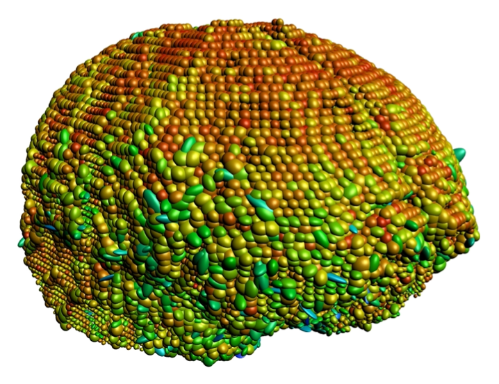
On the modeling side, there has been an increasing interest in manifold-valued data processing: apart from statistical [89, 88, 55, 76] and PDE approaches [73, 35] to smooth data processing on manifolds, non-smooth variational approaches on Riemannian manifolds have been gaining momentum as well in the 2010s. Typical applications include non-linear color spaces [34] such as the Chromaticity Brightness model (S2×superscript𝑆2S^{2}\times\mathbb{R}) and the Hue Saturation Value model (S1×2superscript𝑆1superscript2S^{1}\times\mathbb{R}^{2}), InSAR imaging [84] (S1superscript𝑆1S^{1}), Diffusion Tensor imaging [11] with the manifold of positive definite symmetric 3×3333\times 3 matrices 𝒫(3)𝒫3\mathcal{P}(3) (Fig. 1) and Electron Backscatter Diffraction imaging [4] with the 3D rotation group SO(3)𝑆𝑂3SO(3). Also several branches in data science have become more involved in using the geometry of problems. Examples include sparse principal component analysis, compressed mode analysis in physics, unsupervised feature selection and sparse blind convolution, where in these cases the Stiefel manifold captures all geometric information; see [37] for an overview.

In this work, we consider optimization problems of the form

(1) infp{F(p)+G(Λ(p))},subscriptinfimum𝑝𝐹𝑝𝐺Λ𝑝\inf_{p\in\mathcal{M}}\left\{F(p)+G(\Lambda(p))\right\},

where F:¯:𝐹¯F:\mathcal{M}\rightarrow\overline{\mathbb{R}} and G:𝒩¯:𝐺𝒩¯G:\mathcal{N}\rightarrow\overline{\mathbb{R}} are non-smooth functions mapping into the extended real line ¯:={±}assign¯plus-or-minus\overline{\mathbb{R}}:=\mathbb{R}\cup\{\pm\infty\}, \mathcal{M} and 𝒩𝒩\mathcal{N} are Riemannian manifolds, and Λ:𝒩:Λ𝒩\Lambda:\mathcal{M}\rightarrow\mathcal{N} is differentiable. In variational image processing models, \mathcal{M} will typically be a discretized space of manifold-valued functions, i.e., whose range is restricted to a manifold. This should be contrasted with case where the domain of the unknown function is a manifold, but the range is Euclidean or even scalar-valued, such as when computing quantities on the surface of a 2D or 3D shape. From an optimization viewpoint, the latter is somewhat easier, as – after discretization – the problem boils down to a finite-dimensional Euclidean optimization problem.

Unlike the Euclidean case =msuperscript𝑚\mathcal{M}=\mathbb{R}^{m}, 𝒩=n𝒩superscript𝑛\mathcal{N}=\mathbb{R}^{n}, to our knowledge no intrinsic higher-order solvers with superlinear convergence exist in the manifold-valued case. Our goal is to close this gap.
Refer to caption
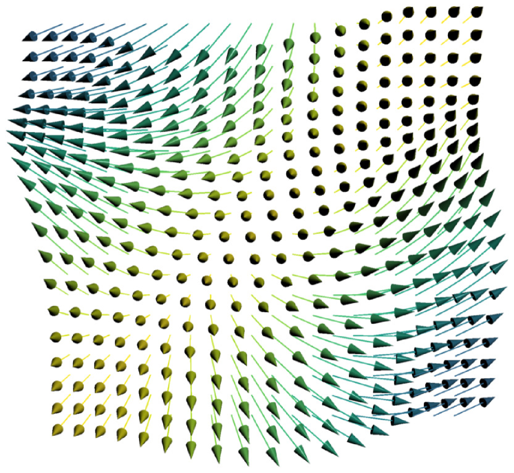
Figure 1: Diffusion-Tensor Magnetic Resonance Imaging (DT-MRI) allows precise fiber tracing in the human brain by modeling the diffusion directions of water molecules using multivariate normal distributions, which are represented by elements on the manifold of symmetric positive definite matrices 𝒫(3)𝒫3\mathcal{P}(3). The resulting optimization problems are manifold-valued and often non-smooth, which necessitates specialized numerical optimization algorithms. Visualization courtesy of [17], based on the Camino data set [42].

1.1 Related Work

There have been multiple attempts to generalize algorithms for both smooth and non-smooth optimization on manifolds. Early work can be traced back to [82], where a manifold constraint is included in the optimization problem and enforced using projections. Using this so-called extrinsic approach, algorithms from the real-valued case can be made to work on manifolds as well, if they can be reasonably embedded into en Euclidean space. While this technique does not capture the manifold structure specifically, recent contributions still tend to this approach for optimization [75, 26, 38, 74, 114]. A step towards exploiting the intrinsic geometry of manifolds is to rely on local charts, which provide a linear subspace in which methods for real-valued optimization can be applied. However, both embedding and localization approaches suffer from serious drawbacks, which are discussed extensively in [61, Sec. 1]. Hence, intrinsic methods that do not rely on charts have become very popular.

Pioneering work using these ideas in smooth optimization on manifolds was done in the 1994 with [97, 102], whose authors formulated several algorithms such as gradient descent, Newton’s method and conjugate gradient on Riemannian manifolds. From then on, the community started working on generalizing other algorithms to Riemannian manifolds [2, 27, 32], specializing algorithms [49, 1, 66] and the application to real-world problems [5, 6]. An extensive overview of first-and second-order methods for smooth optimization on matrix manifolds can be found in [3].

The development of non-smooth Riemannian optimization methods appears to have occurred somewhat independently in the image analysis- and in the non-smooth optimization communities. Whereas the former mostly relied on methods that generalize convexity, the latter has been focussed on finding new notions and restrictions to generalize manifold algorithms from the smooth to non-smooth setting. We give a short survey of both, as we believe that either provide valuable insights.

Manifold-valued Imaging

The non-smooth Rudin-Osher-Fatemi (ROF) model [94] is the prototype of modern image analysis. This model revolves around the notion of Total Variation (TV), which has also been generalized to the S1superscript𝑆1S^{1} manifold in the early 1990s [57] and has been extended to general Riemannian manifolds in the second half of the 2000s [58, 59]. Although early numerical attempts for TV-regularized problems on manifolds originate in the early 2000s [34], the majority of the initial contributions in TV-based models on manifolds were proposed in the early 2010s [100, 43, 104]. These initial models had the major drawback that they were proposed for specific manifolds. In [79], the authors reformulated the variational problem on arbitrary Riemannian manifolds into a multi-label optimization problem. In [107], the generalized ROF model was formulated in a fully intrinsic fashion.

When entering the second half of the 2010s we see generalizations to several models emerging. A second-order model for cyclic data was proposed in [21], and soon, popular real-valued models were extended to the manifold case: a general second-order method [9], infimal convolution models [18, 19], and TGV for manifold-valued imaging [28, 19]. At the same time specialized models were extended to applications such as inpainting [24], segmentation [108], or manifold-valued inverse problems [12, 98]. Additionally, new problem settings arose with the emergence TV for manifold-valued data on graphs [23].

As non-smooth models were extended to manifolds, so did the solvers. The proposed algorithms were typically proposed on Hadamard manifolds: Riemannian manifolds that are complete, simply connected and have non-positive sectional curvature. On these manifolds, convexity can be generalized, which has been crucial in many of the convergence proofs. Proposed algorithms include the Proximal Point Algorithm (PPA) [10] and its extension, the Cyclic Proximal Point Algorithm (CPPA) [8]; Iteratively Reweighted Least Squares (IRLS) [63, 17] and an adaptation in [64]; the Parallel Douglas-Racheford Algorithm (PDRA) [22]; and the recently derived exact and linearized Riemannian Chambolle Pock Algorithms (eRCPA/lRCPA) [20]. Despite the Hadamard constraint, it should be noted that these algorithms perform well on manifolds with positive curvature in experiments. Methods that do not rely on the Hadamard constraint include exact methods as in [99], which uses exact solutions for 1superscript1\ell^{1}-TV with spherical data, and functional lifting [105]. These methods come with their own shortcomings: for the former this is limited applicability and for the latter this is high computational cost.

Non-smooth Optimization on Manifolds

For non-smooth optimization on manifolds, the pioneering works include [53], in which the subgradient method was extended to Riemannian manifolds and was shown to converge on Hadamard manifolds, and [54], whose authors extended the proximal map and proved convergence on Hadamard manifolds. Further development in non-smooth optimization was accelerated in the late 2000s by the introduction of the proximal subdifferential for manifolds [7], the Clarke generalized subdifferential for manifolds [70], and a framework for duality on CAT(0)𝐶𝐴𝑇0CAT(0) metric spaces [72].

By the start of the 2010s, researchers started moving from Hadamard spaces to the non-Hadamard case. New developments include the introduction of a non-smooth version of the Kurdyka-Lojasiewicz (KL) inequality used to show the convergence of PPA on general Riemannian manifolds [14], convergence of subgradient descent for functions satisfying the KL inequality to a singular critical point [68], and a new approach to the convergence of PPA that extends previous results to a broader class of functions [15].

Around 2015, the first numerical implementations of these and new algorithms received attention: [61] introduced a non-smooth trust region method for Riemannian manifolds and showed global convergence, [62] used an approximate subdifferential and proposed a descent method with global convergence, [71] proposed a gradient sampling algorithm and showed its global convergence, and [69] proposed a line search algorithm and generalized the Wolfe conditions for Riemannian manifolds. Recently, a higher-order method was introduced: the Riemannian Semi-smooth Newton method (RSSN) [45], although to our knowledge no publicly-available implementation has existed so far. This method will form the basis of our approach.

1.2 Contribution

The contributions of this work are two-fold:

1. Primal-Dual Riemannian Semi-smooth Newton (PD-RSSN) for non-smooth optimization

While the RSSN method [45] allows to find zeros of generic vector fields on manifolds in the same way that the Newton method allows to solve nonlinear systems of equations, the application to finding minimizers of non-smooth optimization problems is not straightforward, as the optimality conditions typically are in inclusion form. Using the recently proposed generalized Fenchel duality theory on manifolds [20], we construct a primal-dual optimality system in the form of a vector field, which is then solved by RSSN. Overall, this provides a superlinearly convergent primal-dual scheme (PD-RSSN) for non-smooth Riemannian optimization.

2. Expanding the theoretical framework of Riemannian Semi-smooth Newton

As in the classical Newton method, the proposed method requires to solve Newton-type system in each step. For larger-scale problems, solving for the Newton steps exactly is often not efficient. Therefore we propose an inexact version of RSSN and provide a convergence proof (Theorem 4.5). We show that at least linear convergence can be expected in the inexact case. The theoretical results are validated by our numerical experiments on a dual (Huber-) regularized 2superscript2\ell^{2}-TV𝑇𝑉TV denoising model on manifolds with positive and negative sectional curvature: The two-dimensional unit sphere S2superscript𝑆2S^{2} and the manifold of symmetric positive semidefinite 3×3333\times 3 matrices 𝒫(3)𝒫3\mathcal{P}(3). The full source code for the reproducing the experiments in this work is available at

https://github.com/wdiepeveen/Primal-Dual-RSSN.

The central concepts in this work, in particular the extension to the Riemannian setting, were developed by the first author in his thesis [47]. Early considerations in the Euclidean case can be found in the thesis [95].

1.3 Outline

In Section 2, basic notation from differential geometry and Riemannian geometry is covered and the necessary definitions for manifold Fenchel duality theory are discussed along with the resulting non-smooth optimality systems. We also summarize the basic notions necessary for applying the Riemannian Semi-smooth Newton method. In Section 3, we discuss how RSSN can be used to solve the non-smooth optimality system from Section 2, which leads to the proposed PD-RSSN method. In Section 4, we present the inexact Riemannian Semi-smooth Newton method and give a local convergence proof. The application of our method to 2superscript2\ell^{2}-TV-like problems is discussed in Section 5, and numerical results are shown in Section 6. We conclude and summarize in Section 7.

2 Preliminaries

In the first half of this section, the notation from differential and Riemannian geometry is summarized. In the second part, we briefly recapitulate manifold Fenchel duality theory and the Riemannian Semi-smooth Newton method.

2.1 Notation

For details regarding differential geometry and Riemannian geometry, we refer the reader to books such as [78, 96, 31].

We write \mathcal{M} and 𝒩𝒩\mathcal{N} for Riemannian manifolds. The tangent space at p𝑝p\in\mathcal{M} is denoted by 𝒯psubscript𝒯𝑝\mathcal{T}_{p}\mathcal{M} and for tangent vectors we write Xpsubscript𝑋𝑝X_{p} and Yp,subscript𝑌𝑝Y_{p}, or simply X𝑋X and Y𝑌Y. For the tangent bundle we have 𝒯:=p𝒯passign𝒯subscript𝑝subscript𝒯𝑝\mathcal{T}\mathcal{M}:=\bigcup_{p\in\mathcal{M}}\mathcal{T}_{p}\mathcal{M}. Similarly, we write 𝒯psubscriptsuperscript𝒯𝑝\mathcal{T}^{*}_{p}\mathcal{M} for the dual of the tangent space, or cotangent space, ξpsubscript𝜉𝑝\xi_{p} and ηpsubscript𝜂𝑝\eta_{p} or simply ξ𝜉\xi and η𝜂\eta for covectors, and 𝒯:=p𝒯passignsuperscript𝒯subscript𝑝superscriptsubscript𝒯𝑝\mathcal{T^{*}}\mathcal{M}:=\bigcup_{p\in\mathcal{M}}\mathcal{T}_{p}^{*}\mathcal{M} for the cotangent bundle. A cotangent vector ξ𝒯p𝜉superscriptsubscript𝒯𝑝\xi\in\mathcal{T}_{p}^{*}\mathcal{M} acts on a tangent vector X𝒯p𝑋subscript𝒯𝑝X\in\mathcal{T}_{p}\mathcal{M} through the duality pairing ξ,Xp:=ξ(X)assignsubscript𝜉𝑋𝑝𝜉𝑋\langle\xi,X\rangle_{p}:=\xi(X)\in\mathbb{R}. For a mapping Λ:𝒩:Λ𝒩\Lambda:\mathcal{M}\rightarrow\mathcal{N}, we write DpΛ:𝒯p𝒯Λ(p)𝒩:subscript𝐷𝑝Λsubscript𝒯𝑝subscript𝒯Λ𝑝𝒩D_{p}\Lambda:\mathcal{T}_{p}\mathcal{M}\rightarrow\mathcal{T}_{\Lambda(p)}\mathcal{N} for the differential of ΛΛ\Lambda at p𝑝p\in\mathcal{M}.

We assume a Riemannian manifold is equipped with a metric. For some point p𝑝p\in\mathcal{M} the metric tensor is denoted by (,)p:𝒯p×𝒯p:subscript𝑝subscript𝒯𝑝subscript𝒯𝑝(\cdot,\cdot)_{p}:\mathcal{T}_{p}\mathcal{M}\times\mathcal{T}_{p}\mathcal{M}\rightarrow\mathbb{R} and the norm induced by the Riemannian metric is written as p\|\cdot\|_{p}. The Riemannian distance between points p,q𝑝𝑞p,q\in\mathcal{M} is denoted by d(p,q)subscript𝑑𝑝𝑞d_{\mathcal{M}}(p,q). For the open metric ball of radius r>0𝑟0r>0 with center p𝑝p\in\mathcal{M} induced by this distance we write

(2) r(p):={yd(p,q)<r}.assignsubscript𝑟𝑝conditional-set𝑦subscript𝑑𝑝𝑞𝑟\mathcal{B}_{r}(p):=\left\{y\in\mathcal{M}\mid d_{\mathcal{M}}(p,q)<r\right\}.

Through this metric, for p𝑝p\in\mathcal{M} we can define the musical isomorphisms :𝒯p𝒯p:subscript𝒯𝑝superscriptsubscript𝒯𝑝\flat:\mathcal{T}_{p}\mathcal{M}\rightarrow\mathcal{T}_{p}^{*}\mathcal{M} as

(3) X,Yp=(X,Y)p for all Y𝒯psubscriptsuperscript𝑋𝑌𝑝subscript𝑋𝑌𝑝 for all 𝑌subscript𝒯𝑝\langle X^{\flat},Y\rangle_{p}=(X,Y)_{p}\text{ for all }Y\in\mathcal{T}_{p}\mathcal{M}

and its inverse :𝒯p𝒯p:superscriptsubscript𝒯𝑝subscript𝒯𝑝\sharp:\mathcal{T}_{p}^{*}\mathcal{M}\rightarrow\mathcal{T}_{p}\mathcal{M} as

(4) (ξ,X)p=ξ,Xp for all X𝒯p.subscriptsuperscript𝜉𝑋𝑝subscript𝜉𝑋𝑝 for all 𝑋subscript𝒯𝑝(\xi^{\sharp},X)_{p}=\langle\xi,X\rangle_{p}\text{ for all }X\in\mathcal{T}_{p}\mathcal{M}.

The metric can also be used to construct a unique affine connection, the Levi-Civita connection or covariant derivative, which is denoted by ()()subscript\nabla_{(\cdot)}(\cdot). For geodesics γ:[0,1],:𝛾01\gamma:[0,1]\rightarrow\mathcal{M,} we typically write γp,q(t)subscript𝛾𝑝𝑞𝑡\gamma_{p,q}(t) and γp,X(t)subscript𝛾𝑝𝑋𝑡\gamma_{p,X}(t) to denote a minimizing geodesic connecting p,q𝑝𝑞p,q\in\mathcal{M} and a geodesic starting from p𝑝p\in\mathcal{M} with velocity γ˙p,X(0)=X𝒯psubscript˙𝛾𝑝𝑋0𝑋subscript𝒯𝑝\dot{\gamma}_{p,X}(0)=X\in\mathcal{T}_{p}\mathcal{M}. The latter defines the exponential map, which is denoted by expp:𝒢p:subscript𝑝subscript𝒢𝑝\exp_{p}:\mathcal{G}_{p}\rightarrow\mathcal{M} where 𝒢p𝒯psubscript𝒢𝑝subscript𝒯𝑝\mathcal{G}_{p}\subset\mathcal{T}_{p}\mathcal{M} is the set on which γ˙p,X=:expp(X)\dot{\gamma}_{p,X}=:\exp_{p}(X) is defined. Furthermore, if 𝒢p=𝒯psubscript𝒢𝑝subscript𝒯𝑝\mathcal{G}_{p}=\mathcal{T}_{p}\mathcal{M}, the manifold is called complete. For 𝒢p𝒢psubscriptsuperscript𝒢𝑝subscript𝒢𝑝\mathcal{G}^{\prime}_{p}\subset\mathcal{G}_{p} a metric ball with radius rpsubscript𝑟𝑝r_{p} on which exppsubscript𝑝\exp_{p} is a diffeomorphism, the logarithmic map is defined and we denote it by logp:exp(𝒢p)𝒢p:subscript𝑝subscriptsuperscript𝒢𝑝subscriptsuperscript𝒢𝑝\log_{p}:\exp(\mathcal{G}^{\prime}_{p})\rightarrow\mathcal{G}^{\prime}_{p}. This radius rpsubscript𝑟𝑝r_{p} is called the injectivity radius. Importantly, on simply connected, complete Riemannian manifolds with non-positive sectional curvature, the exppsubscript𝑝\exp_{p} and logpsubscript𝑝\log_{p} maps are globally defined. Such manifolds are called Hadamard manifolds. Finally, we write parallel transport of a vector X𝒯p𝑋subscript𝒯𝑝X\in\mathcal{T}_{p}\mathcal{M} from p𝑝p to q𝑞q\in\mathcal{M} as 𝒫qpXsubscript𝒫𝑞𝑝𝑋\mathcal{P}_{q\leftarrow p}X and parallel transport of a covector ξ𝒯p𝜉superscriptsubscript𝒯𝑝\xi\in\mathcal{T}_{p}^{*}\mathcal{M} as 𝒫qpξsubscript𝒫𝑞𝑝𝜉\mathcal{P}_{q\leftarrow p}\xi, where the latter is defined through the musical isomorphisms, as

(5) 𝒫qpξ:=(𝒫qpξ).assignsubscript𝒫𝑞𝑝𝜉superscriptsubscript𝒫𝑞𝑝superscript𝜉\mathcal{P}_{q\leftarrow p}\xi:=\left(\mathcal{P}_{q\leftarrow p}\xi^{\sharp}\right)^{\flat}.

2.2 Manifold Duality Theory

In this section, generalizations of classical notions from non-smooth analysis to manifolds proposed in [20] are discussed. For the equivalent basic notions of convex analysis in vector spaces we refer the reader to [93, 39]. The section culminates in the recently derived primal-dual optimality conditions proposed by the authors of [20]. In the following, ¯:={±}assign¯plus-or-minus\overline{\mathbb{R}}:=\mathbb{R}\cup\{\pm\infty\} denotes the extended real line.

2.2.1 Non-smooth Analysis and a Fenchel Conjugation Scheme on Manifolds

The notion of convexity can be defined on strongly convex subsets of Riemannian manifolds.

Definition 2.1 (strongly convex set, [96, Def. IV.5.1]).

A subset 𝒞𝒞\mathcal{C}\subset\mathcal{M} of a Riemannian manifold \mathcal{M} is said to be strongly convex if, for all p,q𝒞𝑝𝑞𝒞p,q\in\mathcal{C}, a minimal geodesic γp,qsubscript𝛾𝑝𝑞\gamma_{p,q} between p𝑝p and q𝑞q exists, is unique, and lies completely in 𝒞𝒞\mathcal{C}.

The well-known notions of properness, convexity and lower semi-continuity can be generalized as follows.

Definition 2.2 (proper, [20, Def. 2.11.i]).

A function F:¯:𝐹¯F:\mathcal{M}\rightarrow\overline{\mathbb{R}} is proper if domF:={x|F(x)<}assigndom𝐹conditional-set𝑥𝐹𝑥\operatorname{dom}F:=\{x\in\mathcal{M}|F(x)<\infty\}\neq\emptyset and F(x)>𝐹𝑥F(x)>-\infty holds for all x𝑥x\in\mathcal{M}.

Definition 2.3 (convex, [20, Def. 2.11.ii]).

Suppose that 𝒞𝒞\mathcal{C}\subset\mathcal{M} is strongly convex. A proper function F:¯:𝐹¯F:\mathcal{M}\rightarrow\overline{\mathbb{R}} is called (geodesically) convex on 𝒞𝒞\mathcal{C}\subset\mathcal{M} if, for all p,q𝒞,𝑝𝑞𝒞p,q\in\mathcal{C,} the composition Fγp,q(t)𝐹subscript𝛾𝑝𝑞𝑡F\circ\gamma_{p,q}(t) is a convex function on [0,1]01[0,1] in the classical sense.

Definition 2.4 (epigraph, [20, Def. 2.11.iii]).

Suppose that 𝒜𝒜\mathcal{A}\subset\mathcal{M}. The epigraph of a function F:𝒜¯:𝐹𝒜¯F:\mathcal{A}\rightarrow\overline{\mathbb{R}} is defined as

(6) epiF:={(x,α)𝒜×|F(x)α}.assignepi𝐹conditional-set𝑥𝛼𝒜𝐹𝑥𝛼\operatorname{epi}F:=\{(x,\alpha)\in\mathcal{A}\times\mathbb{R}|F(x)\leq\alpha\}.

Definition 2.5 (lower semi-continuous, [20, Def. 2.11.iv]).

Suppose that 𝒜𝒜\mathcal{A}\subset\mathcal{M}. A proper function F:𝒜¯:𝐹𝒜¯F:\mathcal{A}\rightarrow\overline{\mathbb{R}} is called lower semi-continuous (lsc) if epiFepi𝐹\operatorname{epi}F is closed.

The notions of subdifferentials and proximal mappings can also be extended to manifolds using the exponential map and the geodesic distance:

Definition 2.6 (subdifferential,[102, Def. 3.4.4]).

Suppose that 𝒞𝒞\mathcal{C}\subset\mathcal{M} is strongly convex. The subdifferential Fsubscript𝐹\partial_{\mathcal{M}}F on 𝒞𝒞\mathcal{C} of a proper, convex function F:𝒞¯:𝐹𝒞¯F:\mathcal{C}\rightarrow\overline{\mathbb{R}} at a point p𝒞𝑝𝒞p\in\mathcal{C} is defined as

(7) F(p):={ξ𝒯p|F(q)F(p)+ξ,logpqp for all q𝒞}.assignsubscript𝐹𝑝conditional-set𝜉superscriptsubscript𝒯𝑝𝐹𝑞𝐹𝑝subscript𝜉subscript𝑝𝑞𝑝 for all 𝑞𝒞\partial_{\mathcal{M}}F(p):=\left\{\xi\in\mathcal{T}_{p}^{*}\mathcal{M}|F(q)\geq F(p)+\langle\xi,\log_{p}q\rangle_{p}\text{ for all }q\in\mathcal{C}\right\}.

Definition 2.7 (proximal mapping, [54]).

Let \mathcal{M} be a Riemannian manifold, F:¯:𝐹¯F:\mathcal{M}\rightarrow\overline{\mathbb{R}} be proper, and λ>0𝜆0\lambda>0. The proximal map of F𝐹F is defined as

(8) proxλF(p):=argminq{12λd(p,q)2+F(q)}.assignsubscriptprox𝜆𝐹𝑝subscript𝑞12𝜆subscript𝑑superscript𝑝𝑞2𝐹𝑞\operatorname{prox}_{\lambda F}(p):=\arg\min_{q\in\mathcal{M}}\left\{\frac{1}{2\lambda}d_{\mathcal{M}}(p,q)^{2}+F(q)\right\}.

Tangent and cotangent spaces play an important role in the generalization of the Fenchel-dual functions. In this context, well-definedness of the exponential and the logarithmic map is ensured by restricting ourselves to the following subset, which is a localized variant of the pre-image of the exponential map:

Definition 2.8 ([20, Def 2.8]).

Let 𝒞𝒞\mathcal{C}\subset\mathcal{M} and p𝒞𝑝𝒞p\in\mathcal{C}. We define the tangent subset 𝒞,p𝒯psubscript𝒞𝑝subscript𝒯𝑝\mathcal{L}_{\mathcal{C},p}\subset\mathcal{T}_{p}\mathcal{M} as

(9) 𝒞,p:={X𝒯pexppX𝒞 and Xp=d(exppX,p)}.assignsubscript𝒞𝑝conditional-set𝑋subscript𝒯𝑝subscript𝑝𝑋𝒞 and subscriptnorm𝑋𝑝subscript𝑑subscript𝑝𝑋𝑝\mathcal{L}_{\mathcal{C},p}:=\left\{X\in\mathcal{T}_{p}\mathcal{M}\mid\exp_{p}X\in\mathcal{C}\text{ and }\|X\|_{p}=d_{\mathcal{M}}(\exp_{p}X,p)\right\}.

With these basic notions, Fenchel duality theory can be generalized as in [20]. The Fenchel conjugate or Fenchel dual is defined by introducing a base point m𝑚m on the manifold.

Definition 2.9 (m𝑚m-Fenchel conjugate,[20, Def. 3.1]).

Suppose that F:𝒞¯:𝐹𝒞¯F:\mathcal{C}\rightarrow\overline{\mathbb{R}} and m𝒞𝑚𝒞m\in\mathcal{C}. The m𝑚m-Fenchel conjugate of F𝐹F is defined as the function Fm:𝒯p¯:subscriptsuperscript𝐹𝑚superscriptsubscript𝒯𝑝¯F^{*}_{m}:\mathcal{T}_{p}^{*}\mathcal{M}\rightarrow\overline{\mathbb{R}} such that

(10) Fm(ξm):=supXC,m{ξm,XmF(expmX)},ξm𝒯m.formulae-sequenceassignsuperscriptsubscript𝐹𝑚subscript𝜉𝑚subscriptsupremum𝑋subscript𝐶𝑚subscriptsubscript𝜉𝑚𝑋𝑚𝐹subscript𝑚𝑋subscript𝜉𝑚superscriptsubscript𝒯𝑚F_{m}^{*}\left(\xi_{m}\right):=\sup_{X\in\mathcal{L}_{C,m}}\left\{\left\langle\xi_{m},X\right\rangle_{m}-F\left(\exp_{m}X\right)\right\},\quad\xi_{m}\in\mathcal{T}_{m}^{*}\mathcal{M}.

For the Fenchel biconjugate, we can then define the following.

Definition 2.10 ((mm)𝑚superscript𝑚(mm^{\prime})-Fenchel biconjugate, [20, Def. 3.5]).

Suppose that F:𝒞¯:𝐹𝒞¯F:\mathcal{C}\rightarrow\overline{\mathbb{R}} and m,m𝒞𝑚superscript𝑚𝒞m,m^{\prime}\in\mathcal{C}. Then the (mm)𝑚superscript𝑚(mm^{\prime})-Fenchel biconjugate function Fmm:𝒞¯:subscript𝐹𝑚superscript𝑚𝒞¯F_{mm^{\prime}}:\mathcal{C}\rightarrow\overline{\mathbb{R}} is defined as

(11) Fmm(p):=supξm𝒯m{ξm,logmpmFm(𝒫mmξm)},p𝒞.formulae-sequenceassignsuperscriptsubscript𝐹𝑚superscript𝑚absent𝑝subscriptsupremumsubscript𝜉superscript𝑚superscriptsubscript𝒯superscript𝑚subscriptsubscript𝜉superscript𝑚subscriptsuperscript𝑚𝑝superscript𝑚superscriptsubscript𝐹𝑚subscript𝒫𝑚superscript𝑚subscript𝜉superscript𝑚𝑝𝒞F_{mm^{\prime}}^{**}(p):=\sup_{\xi_{m^{\prime}}\in\mathcal{T}_{m^{\prime}}^{*}\mathcal{M}}\left\{\left\langle\xi_{m^{\prime}},\log_{m^{\prime}}p\right\rangle_{m^{\prime}}-F_{m}^{*}\left(\mathcal{P}_{m\leftarrow m^{\prime}}\xi_{m^{\prime}}\right)\right\},\quad p\in\mathcal{C}.

Basic properties and a more elaborate discussion of these generalized conjugate functions are covered in [20]. We will only focus on the relation between Fmmsubscriptsuperscript𝐹absent𝑚𝑚F^{**}_{mm} and F𝐹F.

First, we note that geodesic convexity is often too strong a condition, so a weaker condition is used. Given a set 𝒞𝒞\mathcal{C}\subset\mathcal{M}, m𝒞𝑚𝒞m\in\mathcal{C}, and a function F:𝒞¯,:𝐹𝒞¯F:\mathcal{C}\rightarrow\overline{\mathbb{R}}, we define fm:𝒯m¯:subscript𝑓𝑚subscript𝒯𝑚¯f_{m}:\mathcal{T}_{m}\mathcal{M}\rightarrow\overline{\mathbb{R}} by

(12) fm(X):={F(expmX),X𝒞,m,+,X𝒞,m.assignsubscript𝑓𝑚𝑋cases𝐹subscript𝑚𝑋𝑋subscript𝒞𝑚𝑋subscript𝒞𝑚f_{m}(X):=\left\{\begin{array}[]{cl}F\left(\exp_{m}X\right),&X\in\mathcal{L}_{\mathcal{C},m},\\ +\infty,&X\notin\mathcal{L}_{\mathcal{C},m}.\end{array}\right.

It turns out that one can look at the convexity of the function fm:𝒯m¯:subscript𝑓𝑚subscript𝒯𝑚¯f_{m}:\mathcal{T}_{m}\mathcal{M}\rightarrow\overline{\mathbb{R}} in the usual vector space sense on 𝒯msubscript𝒯𝑚\mathcal{T}_{m}\mathcal{M}. For a more elaborate discussion of the discrepancy between the convexity of fmsubscript𝑓𝑚f_{m} and (geodesic) convexity of F𝐹F we refer to [20, Example 3.10].

Now, the Fenchel-Moreau-Rockafellar theorem can also be extended to the manifold case:

Theorem 2.11 ([20, Thm. 3.13]).

Suppose that 𝒞𝒞\mathcal{C}\subset\mathcal{M} is strongly convex and m𝒞𝑚𝒞m\in\mathcal{C}. Let F:𝒞¯:𝐹𝒞¯F:\mathcal{C}\rightarrow\overline{\mathbb{R}} be proper. If fmsubscript𝑓𝑚f_{m} is lsc and convex on 𝒯m,subscript𝒯𝑚\mathcal{T}_{m}\mathcal{M}, then F=Fmm.𝐹superscriptsubscript𝐹𝑚𝑚absentF=F_{mm}^{**}. In this case Fmsuperscriptsubscript𝐹𝑚F_{m}^{*} is proper as well.

2.2.2 The First-order Optimality Conditions

In this section the first-order optimality conditions for a minimization problem of the form

(13) infp𝒞{F(p)+G(Λ(p))}subscriptinfimum𝑝𝒞𝐹𝑝𝐺Λ𝑝\inf_{p\in\mathcal{C}}\left\{F(p)+G(\Lambda(p))\right\}

are discussed. Here 𝒞𝒞\mathcal{C}\subset\mathcal{M} and 𝒟𝒩𝒟𝒩\mathcal{D}\subset\mathcal{N} are strongly convex sets, F:𝒞¯:𝐹𝒞¯F:\mathcal{C}\rightarrow\overline{\mathbb{R}} and G:𝒟¯:𝐺𝒟¯G:\mathcal{D}\rightarrow\overline{\mathbb{R}} are proper functions, and Λ:𝒩:Λ𝒩\Lambda:\mathcal{M}\rightarrow\mathcal{N} is a differentiable map, possibly nonlinear, such that Λ(𝒞)𝒟Λ𝒞𝒟\Lambda(\mathcal{C})\subset\mathcal{D}. Furthermore, we assume that F:𝒞¯:𝐹𝒞¯F:\mathcal{C}\rightarrow\overline{\mathbb{R}} is geodesically convex and that

(14) gn(X):={G(expnX),X𝒟,n,+,X𝒟,n,assignsubscript𝑔𝑛𝑋cases𝐺subscript𝑛𝑋𝑋subscript𝒟𝑛𝑋subscript𝒟𝑛g_{n}(X):=\left\{\begin{array}[]{cl}G\left(\exp_{n}X\right),&X\in\mathcal{L}_{\mathcal{D},n},\\ +\infty,&X\notin\mathcal{L}_{\mathcal{D},n},\end{array}\right.

is proper, convex and lsc on 𝒯n𝒩subscript𝒯𝑛𝒩\mathcal{T}_{n}\mathcal{N} for some n𝒟𝑛𝒟n\in\mathcal{D}.

Under these assumptions, Eq. 13 can be rewritten into the following saddle-point formulation

(15) infp𝒞supξn𝒯n𝒩{ξn,lognΛ(p)n+F(p)Gn(ξn)}subscriptinfimum𝑝𝒞subscriptsupremumsubscript𝜉𝑛superscriptsubscript𝒯𝑛𝒩subscriptsubscript𝜉𝑛subscript𝑛Λ𝑝𝑛𝐹𝑝superscriptsubscript𝐺𝑛subscript𝜉𝑛\inf_{p\in\mathcal{C}}\sup_{\xi_{n}\in\mathcal{T}_{n}^{*}\mathcal{N}}\left\{\left\langle\xi_{n},\log_{n}\Lambda(p)\right\rangle_{n}+F(p)-G_{n}^{*}\left(\xi_{n}\right)\right\}

The authors of [20] propose two pairs of optimality conditions which we will also refer to as the exact and linearized optimality conditions for the primal and dual variables. The proposed exact optimality conditions are

(16) 𝒫pm((DmΛ)[𝒫Λ(m)nξn])subscript𝒫𝑝𝑚superscriptsubscript𝐷𝑚Λdelimited-[]subscript𝒫Λ𝑚𝑛subscript𝜉𝑛\displaystyle\mathcal{P}_{p\leftarrow m}\left(-(D_{m}\Lambda)^{*}\left[\mathcal{P}_{\Lambda(m)\leftarrow n}\xi_{n}\right]\right) F(p),absentsubscript𝐹𝑝\displaystyle\in\partial_{\mathcal{M}}F(p),
(17) lognΛ(p)subscript𝑛Λ𝑝\displaystyle\log_{n}\Lambda(p) Gn(ξn),absentsuperscriptsubscript𝐺𝑛subscript𝜉𝑛\displaystyle\in\partial G_{n}^{*}\left(\xi_{n}\right),

where DmΛ:𝒯Λ(m)𝒩𝒯m:subscript𝐷𝑚superscriptΛsuperscriptsubscript𝒯Λ𝑚𝒩superscriptsubscript𝒯𝑚D_{m}\Lambda^{*}:\mathcal{T}_{\Lambda(m)}^{*}\mathcal{N}\rightarrow\mathcal{T}_{m}^{*}\mathcal{M} is the adjoint operator of DmΛsubscript𝐷𝑚ΛD_{m}\Lambda. As shown in [20], this system can be rewritten into

(18) p𝑝\displaystyle p =proxσF(expp(𝒫pm(σ(DmΛ)[𝒫Λ(m)nξn]))),absentsubscriptprox𝜎𝐹subscript𝑝subscript𝒫𝑝𝑚superscript𝜎superscriptsubscript𝐷𝑚Λdelimited-[]subscript𝒫Λ𝑚𝑛subscript𝜉𝑛\displaystyle=\operatorname{prox}_{\sigma F}\left(\exp_{p}\left(\mathcal{P}_{p\leftarrow m}\left(-\sigma(D_{m}\Lambda)^{*}\left[\mathcal{P}_{\Lambda(m)\leftarrow n}\xi_{n}\right]\right)^{\sharp}\right)\right),
(19) ξnsubscript𝜉𝑛\displaystyle\xi_{n} =proxτGn(ξn+τ(lognΛ(p))).absentsubscriptprox𝜏subscriptsuperscript𝐺𝑛subscript𝜉𝑛𝜏superscriptsubscript𝑛Λ𝑝\displaystyle=\operatorname{prox}_{\tau G^{*}_{n}}\left(\xi_{n}+\tau\left(\log_{n}\Lambda\left(p\right)\right)^{\flat}\right).

As coined in [103, 20], we use the term “exact” to refer to the fact that the operator ΛΛ\Lambda is used in its original form in without linearization in Eq. 19. However, note that the linearization

(20) Λ(p)expΛ(m)DΛ(m)[logmp]Λ𝑝subscriptΛ𝑚𝐷Λ𝑚delimited-[]subscript𝑚𝑝\Lambda(p)\approx\exp_{\Lambda(m)}D\Lambda(m)\left[\log_{m}p\right]

was still needed to obtain Eq. 16, in particular so that the adjoint operator DmΛsubscript𝐷𝑚ΛD_{m}\Lambda can be constructed.

The linearized optimality conditions can be obtained by linearizing both the primal and the dual optimality condition. That is, for n:=Λ(m),assign𝑛Λ𝑚n:=\Lambda(m), we want to solve

(21) infpinfξn𝒯n𝒩{F(p)+ξn,DmΛ[logmp]nGn(ξn)},subscriptinfimum𝑝subscriptinfimumsubscript𝜉𝑛superscriptsubscript𝒯𝑛𝒩𝐹𝑝subscriptsubscript𝜉𝑛subscript𝐷𝑚Λdelimited-[]subscript𝑚𝑝𝑛superscriptsubscript𝐺𝑛subscript𝜉𝑛\inf_{p\in\mathcal{M}}\inf_{\xi_{n}\in\mathcal{T}_{n}^{*}\mathcal{N}}\{F(p)+\left\langle\xi_{n},D_{m}\Lambda\left[\log_{m}p\right]\right\rangle_{n}-G_{n}^{*}\left(\xi_{n}\right)\},

and obtain the optimality system for the general n𝒩𝑛𝒩n\in\mathcal{N} case [20]

(22) 𝒫pm((DmΛ)[𝒫Λ(m)nξn])subscript𝒫𝑝𝑚superscriptsubscript𝐷𝑚Λdelimited-[]subscript𝒫Λ𝑚𝑛subscript𝜉𝑛\displaystyle\mathcal{P}_{p\leftarrow m}\left(-(D_{m}\Lambda)^{*}\left[\mathcal{P}_{\Lambda(m)\leftarrow n}\xi_{n}\right]\right) F(p),absentsubscript𝐹𝑝\displaystyle\in\partial_{\mathcal{M}}F(p),
(23) DmΛ[logmp]subscript𝐷𝑚Λdelimited-[]subscript𝑚𝑝\displaystyle D_{m}\Lambda\left[\log_{m}p\right] Gn(ξn),absentsuperscriptsubscript𝐺𝑛subscript𝜉𝑛\displaystyle\in\partial G_{n}^{*}\left(\xi_{n}\right),

which can be rewritten into

(24) p𝑝\displaystyle p =proxσF(expp(𝒫pm(σ(DmΛ)[𝒫Λ(m)nξn]))),absentsubscriptprox𝜎𝐹subscript𝑝subscript𝒫𝑝𝑚superscript𝜎superscriptsubscript𝐷𝑚Λdelimited-[]subscript𝒫Λ𝑚𝑛subscript𝜉𝑛\displaystyle=\operatorname{prox}_{\sigma F}\left(\exp_{p}\left(\mathcal{P}_{p\leftarrow m}\left(-\sigma\left(D_{m}\Lambda\right)^{*}\left[\mathcal{P}_{\Lambda(m)\leftarrow n}\xi_{n}\right]\right)^{\sharp}\right)\right),
(25) ξnsubscript𝜉𝑛\displaystyle\xi_{n} =proxτGn(ξn+τ(𝒫nΛ(m)DmΛ[logmp])).absentsubscriptprox𝜏superscriptsubscript𝐺𝑛subscript𝜉𝑛𝜏superscriptsubscript𝒫𝑛Λ𝑚subscript𝐷𝑚Λdelimited-[]subscript𝑚𝑝\displaystyle=\operatorname{prox}_{\tau G_{n}^{*}}\left(\xi_{n}+\tau\left(\mathcal{P}_{n\leftarrow\Lambda(m)}D_{m}\Lambda\left[\log_{m}p\right]\right)^{\flat}\right).

We note that the connection between the linearized optimality conditions and a solution of the original problem has only been conclusively established in the Euclidean case so far [103]. In the Riemannian case, the following weak duality result holds:

Theorem 2.12 ([20, Thm. 4.2]).

Let n:=Λ(m)assign𝑛Λ𝑚n:=\Lambda(m). The dual problem of

(26) infp{F(p)+G(expΛ(m)DmΛ[logmp])}subscriptinfimum𝑝𝐹𝑝𝐺subscriptΛ𝑚subscript𝐷𝑚Λdelimited-[]subscript𝑚𝑝\inf_{p\in\mathcal{M}}\left\{F(p)+G(\exp_{\Lambda(m)}D_{m}\Lambda\left[\log_{m}p\right])\right\}

is given by

(27) supξn𝒯n𝒩{Fm((DmΛ)[ξn])Gn(ξn)}subscriptsupremumsubscript𝜉𝑛superscriptsubscript𝒯𝑛𝒩superscriptsubscript𝐹𝑚superscriptsubscript𝐷𝑚Λdelimited-[]subscript𝜉𝑛superscriptsubscript𝐺𝑛subscript𝜉𝑛\sup_{\xi_{n}\in\mathcal{T}_{n}^{*}\mathcal{N}}\left\{F_{m}^{*}\left(-(D_{m}\Lambda)^{*}\left[\xi_{n}\right]\right)-G_{n}^{*}\left(\xi_{n}\right)\right\}

and weak duality holds, i.e.,

(28) infp{F(p)+G(expΛ(m)DmΛ[logmp])}supξn𝒯n𝒩{Fm((DmΛ)[ξn])Gn(ξn)}.subscriptinfimum𝑝𝐹𝑝𝐺subscriptΛ𝑚subscript𝐷𝑚Λdelimited-[]subscript𝑚𝑝subscriptsupremumsubscript𝜉𝑛subscriptsuperscript𝒯𝑛𝒩superscriptsubscript𝐹𝑚superscriptsubscript𝐷𝑚Λdelimited-[]subscript𝜉𝑛superscriptsubscript𝐺𝑛subscript𝜉𝑛\inf_{p\in\mathcal{M}}\left\{F(p)+G(\exp_{\Lambda(m)}D_{m}\Lambda\left[\log_{m}p\right])\right\}\geq\sup_{\xi_{n}\in\mathcal{T}^{*}_{n}\mathcal{N}}\left\{-F_{m}^{*}\left(-(D_{m}\Lambda)^{*}\left[\xi_{n}\right]\right)-G_{n}^{*}\left(\xi_{n}\right)\right\}.

If one performs a suitable fixed-point iteration on Eqs. 24 and 25, one obtains the linearized Riemannian Chambolle Pock algorithm, which has been shown to converge on Hadamard manifolds [20, Thm. 4.3]. In this work, we aim to construct a higher-order method instead.

2.3 The Riemannian Semi-smooth Newton Method

This section is devoted to the Riemannian Semi-smooth Newton (RSSN) method, which we propose to use for solving Eq. 13.

Remark 2.13.

Throughout this section and Section 4, we will develop RSSN on some manifold superscript\mathcal{M}^{\prime}. This is not the original manifold \mathcal{M} defining the feasible set;  we will later apply the RSSN method to =×𝒯n𝒩superscriptsubscriptsuperscript𝒯𝑛𝒩\mathcal{M}^{\prime}=\mathcal{M}\times\mathcal{T}^{*}_{n}\mathcal{N} (and p=(p,ξn)superscript𝑝𝑝subscript𝜉𝑛p^{\prime}=(p,\xi_{n})). In order not to clutter the notation, we still write \mathcal{M} instead of superscript\mathcal{M}^{\prime} (and p𝑝p instead of psuperscript𝑝p^{\prime}) throughout this section and Section 4.

In the real-valued case, the Newton method is formulated for solving a smooth system of equations X(p)=0𝑋𝑝0X(p)=0 for some non-linear map X:dd:𝑋superscript𝑑superscript𝑑X:\mathbb{R}^{d}\rightarrow\mathbb{R}^{d}, where – in the optimization context – this map implements optimality conditions for the minimization problem. In the real-valued case, the classical Newton iteration is given by

(29) pk+1=pkX(pk)1X(pk).superscript𝑝𝑘1superscript𝑝𝑘𝑋superscriptsuperscript𝑝𝑘1𝑋superscript𝑝𝑘p^{k+1}=p^{k}-\nabla X(p^{k})^{-1}X(p^{k}).

In the manifold case, there is no unique generalization. One possibility is to consider a vector field X:𝒯:𝑋𝒯X:\mathcal{M}\rightarrow\mathcal{T}\mathcal{M} and define the Newton iteration through the covariant derivative:

(30) pk+1=exppk([()X]pk1X(pk))superscript𝑝𝑘1subscriptsuperscript𝑝𝑘superscriptsubscriptdelimited-[]subscript𝑋superscript𝑝𝑘1𝑋superscript𝑝𝑘p^{k+1}=\exp_{p^{k}}(-[\nabla_{(\cdot)}X]_{p^{k}}^{-1}X(p^{k}))

in order to find a zero 0=X(p)0𝑋𝑝0=X(p) of the vector field. In this section, we will focus on a generalized covariant derivative approach for finding zeros of semi-smooth vector fields based on Eq. 24Eq. 25. Throughout this section we will use the notions and results developed in [45].

Definition 2.14 ((locally) Lipschitz, [45, Def. 6]).

A vector field X𝑋X on \mathcal{M} is said to be Lipschitz continuous on ΩΩ\Omega\subset\mathcal{M} if there exists a constant L>0𝐿0L>0 such that, for all p,qΩ𝑝𝑞Ωp,q\in\Omega, there holds

(31) 𝒫qpX(p)X(q)qLd(p,q),p,qΩ,formulae-sequencesubscriptnormsubscript𝒫𝑞𝑝𝑋𝑝𝑋𝑞𝑞𝐿subscript𝑑𝑝𝑞for-all𝑝𝑞Ω\left\|\mathcal{P}_{q\leftarrow p}X(p)-X(q)\right\|_{q}\leq Ld_{\mathcal{M}}(p,q),\quad\forall p,q\in\Omega,

Moreover, for a point p𝑝p\in\mathcal{M}, if there exists δ>0𝛿0\delta>0 such that X𝑋X is Lipschitz continuous on the open ball Bδ(p),subscript𝐵𝛿𝑝B_{\delta}(p), then X𝑋X is said to be Lipschitz continuous at p. Moreover, if for all p𝑝p\in\mathcal{M}, X𝑋X is Lipschitz continuous at p𝑝p, then X𝑋X is said to be locally Lipschitz continuous on \mathcal{M}.

Subsequently, we can generalize Rademacher’s theorem to Lipschitz vector fields.

Theorem 2.15 ([45, Thm. 10]).

If X𝑋X is a locally Lipschitz continuous vector field on \mathcal{M}, then X𝑋X is almost everywhere differentiable on \mathcal{M}.

Hence, it makes sense to define the generalized covariant derivative.

Definition 2.16 (Clarke generalized covariant derivative, [45, Def. 11]).

The Clarke generalized covariant derivative CXsubscript𝐶𝑋\partial_{C}X of a locally Lipschitz continuous vector field X𝑋X at a point p𝑝p\in\mathcal{M} is defined as the set-valued mapping CX(p):𝒯p𝒯p:subscript𝐶𝑋𝑝subscript𝒯𝑝subscript𝒯𝑝\partial_{C}X\left(p\right):\mathcal{T}_{p}\mathcal{M}\rightrightarrows\mathcal{T}_{p}\mathcal{M},

(32) CX(p):=co{V(𝒯p):(pk)k0𝒟X,limkpk=p,V=limk𝒫ppkX(pk)},assignsubscript𝐶𝑋𝑝co:𝑉subscript𝒯𝑝formulae-sequencesubscriptsuperscript𝑝𝑘𝑘0subscript𝒟𝑋formulae-sequencesubscript𝑘superscript𝑝𝑘𝑝𝑉subscript𝑘subscript𝒫𝑝superscript𝑝𝑘𝑋superscript𝑝𝑘\partial_{C}X\left(p\right):=\operatorname{co}\left\{V\in\mathcal{L}\left(\mathcal{T}_{p}\mathcal{M}\right):\exists(p^{k})_{k\geq 0}\subset\mathcal{D}_{X},\lim_{k\rightarrow\infty}p^{k}=p,\;V=\lim_{k\rightarrow\infty}\mathcal{P}_{p\leftarrow p^{k}}\nabla X(p^{k})\right\},

where 𝒟Xsubscript𝒟𝑋\mathcal{D}_{X}\subset\mathcal{M} is the set on which X𝑋X is differentiable, “co” represents the convex hull and (𝒯p)subscript𝒯𝑝\mathcal{L}\left(\mathcal{T}_{p}\mathcal{M}\right) is the vector space consisting of all bounded linear operators from 𝒯psubscript𝒯𝑝\mathcal{T}_{p}\mathcal{M} to 𝒯psubscript𝒯𝑝\mathcal{T}_{p}\mathcal{M}.

In addition to local Lipschitzness, we will also need the directional derivative for the notion of semi-smoothness. We follow the definition in [45].

Definition 2.17 (directional derivative).

The directional derivative of a vector field X𝑋X on \mathcal{M} at p𝑝p\in\mathcal{M} in the direction v𝒯p𝑣subscript𝒯𝑝v\in\mathcal{T}_{p}\mathcal{M} is defined by

(33) X(p,v):=limt01t[𝒫pexpp(tv)X(expp(tv))X(p)]𝒯p,assignsuperscript𝑋𝑝𝑣subscript𝑡01𝑡delimited-[]subscript𝒫𝑝subscript𝑝𝑡𝑣𝑋subscript𝑝𝑡𝑣𝑋𝑝subscript𝒯𝑝X^{\prime}(p,v):=\lim_{t\searrow 0}\frac{1}{t}\left[\mathcal{P}_{p\leftarrow\exp_{p}(tv)}X\left(\exp_{p}(tv)\right)-X(p)\right]\in\mathcal{T}_{p}\mathcal{M},

whenever the limit exists. If this directional derivative exists for every v𝑣v, then X𝑋X is said to be directionally differentiable at p𝑝p.

Finally, we are able to generalize the notion of semi-smoothness to vector fields.

Definition 2.18 (semi-smooth vector field, [45, Def. 18]).

A vector field X𝑋X on \mathcal{M} that is Lipschitz continuous at p𝑝p\in\mathcal{M} and directionally differentiable at qBδ(p)𝑞subscript𝐵𝛿𝑝q\in B_{\delta}\left(p\right) for all directions in 𝒯psubscript𝒯𝑝\mathcal{T}_{p}\mathcal{M}, is said to be semi-smooth at p𝑝p iff for every ϵ>0italic-ϵ0\epsilon>0 there exists 0<δ<rp0𝛿subscript𝑟𝑝0<\delta<r_{p}, where rpsubscript𝑟𝑝r_{p} is the injectivity radius, such that

(34) X(p)𝒫pq[X(q)+Vqlogqp]pϵd(p,q),qBδ(p),VqCX(q).formulae-sequencesubscriptnorm𝑋𝑝subscript𝒫𝑝𝑞delimited-[]𝑋𝑞subscript𝑉𝑞subscript𝑞𝑝𝑝italic-ϵsubscript𝑑𝑝𝑞formulae-sequencefor-all𝑞subscript𝐵𝛿𝑝for-allsubscript𝑉𝑞subscript𝐶𝑋𝑞\|X\left(p\right)-\mathcal{P}_{p\leftarrow q}\left[X(q)+V_{q}\log_{q}p\right]\|_{p}\leq\epsilon d_{\mathcal{M}}\left(p,q\right),\quad\forall q\in B_{\delta}\left(p\right),\quad\forall V_{q}\in\partial_{C}X(q).

The vector field X𝑋X is said to be μ𝜇\mu-order semi-smooth at p𝑝p for 0<μ10𝜇10<\mu\leq 1 iff there exist ϵ>0italic-ϵ0\epsilon>0 and 0<δ<rp0𝛿subscript𝑟𝑝0<\delta<r_{p} such that

(35) X(p)𝒫pq[X(q)+Vqlogqp]pϵd(p,q)1+μ,qBδ(p),VqCX(q).formulae-sequencesubscriptnorm𝑋𝑝subscript𝒫𝑝𝑞delimited-[]𝑋𝑞subscript𝑉𝑞subscript𝑞𝑝𝑝italic-ϵsubscript𝑑superscript𝑝𝑞1𝜇formulae-sequencefor-all𝑞subscript𝐵𝛿𝑝for-allsubscript𝑉𝑞subscript𝐶𝑋𝑞\|X\left(p\right)-\mathcal{P}_{p\leftarrow q}\left[X(q)+V_{q}\log_{q}p\right]\|_{p}\leq\epsilon d_{\mathcal{M}}\left(p,q\right)^{1+\mu},\quad\forall q\in B_{\delta}\left(p\right),\quad\forall V_{q}\in\partial_{C}X(q).

The Riemannian Semi-smooth Newton method for finding a zero of a vector field, i.e., X(p)=0𝑋𝑝0X(p)=0, is shown in Algorithm 1. It extends on the classical Newton method by replacing the classical Jacobian X(pk)𝑋superscript𝑝𝑘\nabla X(p^{k}) by an element from the Clarke generalized covariant derivative CX(pk)subscript𝐶𝑋superscript𝑝𝑘\partial_{C}X(p^{k}), and performing the update step using the exponential map.

Algorithm 1 Riemannian Semi-smooth Newton
  Initialization: p0,k:=0formulae-sequencesuperscript𝑝0assign𝑘0p^{0}\in\mathcal{M},k:=0
  while not converged do
     Choose any V(pk)CX(pk)𝑉superscript𝑝𝑘subscript𝐶𝑋superscript𝑝𝑘V(p^{k})\in\partial_{C}X(p^{k})
     Solve V(pk)dk=X(pk)𝑉superscript𝑝𝑘superscript𝑑𝑘𝑋superscript𝑝𝑘V(p^{k})d^{k}=-X(p^{k}) in the vector space 𝒯pksubscript𝒯superscript𝑝𝑘\mathcal{T}_{p^{k}}\mathcal{M}
     pk+1:=exppk(dk)assignsuperscript𝑝𝑘1subscriptsuperscript𝑝𝑘superscript𝑑𝑘p^{k+1}:=\exp_{p^{k}}(d^{k})
     k:=k+1assign𝑘𝑘1k:=k+1
  end while

We have the following local convergence result.

Theorem 2.19 ([45, Thm. 19]).

Let X𝑋X be a locally Lipschitz-continuous vector field on \mathcal{M} and psuperscript𝑝p^{*}\in\mathcal{M} be a solution of the problem X(p)=0𝑋𝑝0X(p)=0. Assume that X𝑋X is semi-smooth at psuperscript𝑝p^{*} and that all VpCX(p)subscript𝑉superscript𝑝subscript𝐶𝑋superscript𝑝V_{p^{*}}\in\partial_{C}X(p^{*}) are invertible. Then there exists a δ>0𝛿0\delta>0 such that, for every starting point p0Bδ(p)\{p}superscript𝑝0\subscript𝐵𝛿superscript𝑝superscript𝑝p^{0}\in B_{\delta}\left(p^{*}\right)\backslash\left\{p^{*}\right\}, the sequence (pk)k0subscriptsuperscript𝑝𝑘𝑘0(p^{k})_{k\geq 0} generated by Algorithm 1 is well-defined, contained in Bδ(p)subscript𝐵𝛿superscript𝑝B_{\delta}\left(p^{*}\right) and converges superlinearly to psuperscript𝑝p^{*}. If additionally X𝑋X is μ𝜇\mu-order semi-smooth at p,superscript𝑝p^{*}, then the convergence of (pk)k0subscriptsuperscript𝑝𝑘𝑘0(p^{k})_{k\geq 0} to psuperscript𝑝p^{*} is of order 1+μ1𝜇1+\mu.

3 A Higher-order Primal-dual Method for Manifolds (PD-RSSN)

We will now merge the ideas of Riemannian Semi-smooth Newton (RSSN) and Fenchel duality theory on manifolds in order to solve the original problem

(36) infp{F(p)+G(Λ(p))}.subscriptinfimum𝑝𝐹𝑝𝐺Λ𝑝\inf_{p\in\mathcal{M}}\{F(p)+G(\Lambda(p))\}.

Using linearization, we saw in Section 2.2 that solving Eq. 36 can be approximated by solving

(37) infpsupξn𝒯n𝒩{F(p)+ξn,DmΛ[logmp]nGn(ξn)},subscriptinfimum𝑝subscriptsupremumsubscript𝜉𝑛superscriptsubscript𝒯𝑛𝒩𝐹𝑝subscriptsubscript𝜉𝑛subscript𝐷𝑚Λdelimited-[]subscript𝑚𝑝𝑛superscriptsubscript𝐺𝑛subscript𝜉𝑛\inf_{p\in\mathcal{M}}\sup_{\xi_{n}\in\mathcal{T}_{n}^{*}\mathcal{N}}\{F(p)+\left\langle\xi_{n},D_{m}\Lambda\left[\log_{m}p\right]\right\rangle_{n}-G_{n}^{*}\left(\xi_{n}\right)\},

which is characterized by the optimality conditions

(38) p𝑝\displaystyle p =proxσF(expp(𝒫pm(σ(DmΛ)[𝒫Λ(m)nξn]))),absentsubscriptprox𝜎𝐹subscript𝑝subscript𝒫𝑝𝑚superscript𝜎superscriptsubscript𝐷𝑚Λdelimited-[]subscript𝒫Λ𝑚𝑛subscript𝜉𝑛\displaystyle=\operatorname{prox}_{\sigma F}\left(\exp_{p}\left(\mathcal{P}_{p\leftarrow m}\left(-\sigma\left(D_{m}\Lambda\right)^{*}\left[\mathcal{P}_{\Lambda(m)\leftarrow n}\xi_{n}\right]\right)^{\sharp}\right)\right),
(39) ξnsubscript𝜉𝑛\displaystyle\xi_{n} =proxτGn(ξn+τ(𝒫nΛ(m)DmΛ[logmp])),absentsubscriptprox𝜏superscriptsubscript𝐺𝑛subscript𝜉𝑛𝜏superscriptsubscript𝒫𝑛Λ𝑚subscript𝐷𝑚Λdelimited-[]subscript𝑚𝑝\displaystyle=\operatorname{prox}_{\tau G_{n}^{*}}\left(\xi_{n}+\tau\left(\mathcal{P}_{n\leftarrow\Lambda(m)}D_{m}\Lambda\left[\log_{m}p\right]\right)^{\flat}\right),

where σ,τ>0𝜎𝜏0\sigma,\tau>0. In this section we focus on rewriting this system of non-linear equations into a form that is amenable to the Riemannian Semi-smooth Newton method, i.e., into the problem of finding a zero of a vector field.

While the dual variable ξnsubscript𝜉𝑛\xi_{n} lives in a vector space and (39) immediately translates into

(40) ξnproxτGn(ξn+τ(𝒫nΛ(m)DmΛ[logmp]))=0,subscript𝜉𝑛subscriptprox𝜏superscriptsubscript𝐺𝑛subscript𝜉𝑛𝜏superscriptsubscript𝒫𝑛Λ𝑚subscript𝐷𝑚Λdelimited-[]subscript𝑚𝑝0\xi_{n}-\operatorname{prox}_{\tau G_{n}^{*}}\left(\xi_{n}+\tau\left(\mathcal{P}_{n\leftarrow\Lambda(m)}D_{m}\Lambda\left[\log_{m}p\right]\right)^{\flat}\right)=0,

the primal optimality condition (38) is an equation in \mathcal{M}. In order to obtain a vector field form, we apply the logarithm, which yields elements from the tangent bundle 𝒯𝒯\mathcal{T}\mathcal{M}:

(41) logpproxσF(expp(𝒫pm(σ(DmΛ)[𝒫Λ(m)nξn])))=0.subscript𝑝subscriptprox𝜎𝐹subscript𝑝subscript𝒫𝑝𝑚superscript𝜎superscriptsubscript𝐷𝑚Λdelimited-[]subscript𝒫Λ𝑚𝑛subscript𝜉𝑛0-\log_{p}\operatorname{prox}_{\sigma F}\left(\exp_{p}\left(\mathcal{P}_{p\leftarrow m}\left(-\sigma\left(D_{m}\Lambda\right)^{*}\left[\mathcal{P}_{\Lambda\left(m\right)\leftarrow n}\xi_{n}\right]\right)^{\sharp}\right)\right)=0.

Such a zero implies Eq. 38. Then, we define the vector field X:×𝒯n𝒩𝒯×𝒯n𝒩:𝑋superscriptsubscript𝒯𝑛𝒩𝒯superscriptsubscript𝒯𝑛𝒩X:\mathcal{M}\times\mathcal{T}_{n}^{*}\mathcal{N}\rightarrow\mathcal{T}\mathcal{M}\times\mathcal{T}_{n}^{*}\mathcal{N} as

(42) X(p,ξn):=(logpproxσF(expp(𝒫pm(σ(DmΛ)[𝒫Λ(m)nξn])))ξnproxτGn(ξn+τ(𝒫nΛ(m)DmΛ[logmp]))).assign𝑋𝑝subscript𝜉𝑛matrixsubscript𝑝subscriptprox𝜎𝐹subscript𝑝subscript𝒫𝑝𝑚superscript𝜎superscriptsubscript𝐷𝑚Λdelimited-[]subscript𝒫Λ𝑚𝑛subscript𝜉𝑛subscript𝜉𝑛subscriptprox𝜏superscriptsubscript𝐺𝑛subscript𝜉𝑛𝜏superscriptsubscript𝒫𝑛Λ𝑚subscript𝐷𝑚Λdelimited-[]subscript𝑚𝑝X(p,\xi_{n}):=\begin{pmatrix}-\log_{p}\operatorname{prox}_{\sigma F}\left(\exp_{p}\left(\mathcal{P}_{p\leftarrow m}\left(-\sigma\left(D_{m}\Lambda\right)^{*}\left[\mathcal{P}_{\Lambda\left(m\right)\leftarrow n}\xi_{n}\right]\right)^{\sharp}\right)\right)\\ \xi_{n}-\operatorname{prox}_{\tau G_{n}^{*}}\left(\xi_{n}+\tau\left(\mathcal{P}_{n\leftarrow\Lambda\left(m\right)}D_{m}\Lambda\left[\log_{m}p\right]\right)^{\flat}\right)\end{pmatrix}.

which allows to apply RSSN. We refer to this approach as Primal-Dual Riemannian Semi-smooth Newton (PD-RSSN).

Remark 3.1.

Here it becomes obvious why first transforming the set-valued equivalent optimality conditions in Eqs. 24 and 25 into the prox-based equality form is crucial: we can now differentiate X𝑋X in order to apply the Newton-based RSSN method.

If the vector field X𝑋X in Eq. 42 is smooth, we obtain the covariant derivative [47, Sec. 6.4.2] at (Yp,ηξn)𝒯p×𝒯n𝒩subscript𝑌𝑝subscript𝜂subscript𝜉𝑛subscript𝒯𝑝superscriptsubscript𝒯𝑛𝒩(Y_{p},\eta_{\xi_{n}})\in\mathcal{T}_{p}\mathcal{M}\times\mathcal{T}_{n}^{*}\mathcal{N}:

(Yp,ηξn)X=(Yplog()f1(p,ξn)Dplogpf1(,ξn)[Yp]Dξnlogpf1(p,)[ηξn]Dpf2(,ξn)[Yp]+ηξnηξnf2(p,)),subscriptsubscript𝑌𝑝subscript𝜂subscript𝜉𝑛𝑋matrixsubscriptsubscript𝑌𝑝subscriptsubscript𝑓1𝑝subscript𝜉𝑛subscript𝐷𝑝subscript𝑝subscript𝑓1subscript𝜉𝑛delimited-[]subscript𝑌𝑝subscript𝐷subscript𝜉𝑛subscript𝑝subscript𝑓1𝑝delimited-[]subscript𝜂subscript𝜉𝑛subscript𝐷𝑝subscript𝑓2subscript𝜉𝑛delimited-[]subscript𝑌𝑝subscript𝜂subscript𝜉𝑛subscriptsubscript𝜂subscript𝜉𝑛subscript𝑓2𝑝\displaystyle\nabla_{(Y_{p},\eta_{\xi_{n}})}X=\begin{pmatrix}-\nabla_{Y_{p}}\log_{(\cdot)}f_{1}(p,\xi_{n})-D_{p}\log_{p}f_{1}(\cdot,\xi_{n})[Y_{p}]-D_{\xi_{n}}\log_{p}f_{1}(p,\cdot)[\eta_{\xi_{n}}]\\ -D_{p}f_{2}(\cdot,\xi_{n})[Y_{p}]+\eta_{\xi_{n}}-\nabla_{\eta_{\xi_{n}}}f_{2}(p,\cdot)\end{pmatrix},

where

(43) f1(p,ξn)subscript𝑓1𝑝subscript𝜉𝑛\displaystyle f_{1}(p,\xi_{n}) :=proxσF(expp(𝒫pm(σ(DmΛ)[𝒫Λ(m)nξn]))),assignabsentsubscriptprox𝜎𝐹subscript𝑝subscript𝒫𝑝𝑚superscript𝜎superscriptsubscript𝐷𝑚Λdelimited-[]subscript𝒫Λ𝑚𝑛subscript𝜉𝑛\displaystyle:=\operatorname{prox}_{\sigma F}\left(\exp_{p}\left(\mathcal{P}_{p\leftarrow m}\left(-\sigma\left(D_{m}\Lambda\right)^{*}\left[\mathcal{P}_{\Lambda\left(m\right)\leftarrow n}\xi_{n}\right]\right)^{\sharp}\right)\right),
(44) f2(p,ξn)subscript𝑓2𝑝subscript𝜉𝑛\displaystyle f_{2}(p,\xi_{n}) :=proxτGn(ξn+τ(𝒫nΛ(m)DmΛ[logmp])).assignabsentsubscriptprox𝜏superscriptsubscript𝐺𝑛subscript𝜉𝑛𝜏superscriptsubscript𝒫𝑛Λ𝑚subscript𝐷𝑚Λdelimited-[]subscript𝑚𝑝\displaystyle:=\operatorname{prox}_{\tau G_{n}^{*}}\left(\xi_{n}+\tau\left(\mathcal{P}_{n\leftarrow\Lambda\left(m\right)}D_{m}\Lambda\left[\log_{m}p\right]\right)^{\flat}\right).

However, we generally cannot assume smoothness of X𝑋X and therefore require a generalization of the differential. First, consider the following generalization of Rademacher’s theorem.

Theorem 3.2.

Let \mathcal{M} and 𝒩𝒩\mathcal{N} be smooth manifolds. If F:𝒩:𝐹𝒩F:\mathcal{M}\rightarrow\mathcal{N} is a locally Lipschitz continuous function, then F𝐹F is almost everywhere differentiable on \mathcal{M}.

Proof 3.3.

The proof is the same as [45, Thm. 10] with a general manifold 𝒩𝒩\mathcal{N} instead of 𝒯𝒯\mathcal{T}\mathcal{M}.

The generalized differential can now be defined as follows; see [70] for a related definition in the more restricted case of functions mapping from a manifold into the real values:

Definition 3.4 (Clarke generalized differential).

The Clarke generalized differential DCFsubscript𝐷𝐶𝐹D_{C}F of a locally Lipschitz continuous function F:𝒩:𝐹𝒩F:\mathcal{M}\rightarrow\mathcal{N} at p𝑝p\in\mathcal{M} is defined as the set-valued mapping DCF(p):𝒯p𝒯F(p)𝒩:subscript𝐷𝐶𝐹𝑝subscript𝒯𝑝subscript𝒯𝐹𝑝𝒩D_{C}F(p):\mathcal{T}_{p}\mathcal{M}\rightrightarrows\mathcal{T}_{F(p)}\mathcal{N},

(45) DCF(p):=co{V(𝒯p,𝒯F(p)𝒩):(pk)k0𝒟F,limkpk=p,V=limkDpkF},assignsubscript𝐷𝐶𝐹𝑝co:𝑉subscript𝒯𝑝subscript𝒯𝐹𝑝𝒩formulae-sequencesubscriptsuperscript𝑝𝑘𝑘0subscript𝒟𝐹formulae-sequencesubscript𝑘superscript𝑝𝑘𝑝𝑉subscript𝑘subscript𝐷superscript𝑝𝑘𝐹D_{C}F(p):=\operatorname{co}\left\{V\in\mathcal{L}\left(\mathcal{T}_{p}\mathcal{M},\mathcal{T}_{F(p)}\mathcal{N}\right):\exists(p^{k})_{k\geq 0}\subset\mathcal{D}_{F},\lim_{k\rightarrow\infty}p^{k}=p,\;V=\lim_{k\rightarrow\infty}D_{p^{k}}F\right\},

where 𝒟Fsubscript𝒟𝐹\mathcal{D}_{F}\subset\mathcal{M} is the set on which F𝐹F is differentiable, “co” represents the convex hull and (𝒯p,𝒯F(p)𝒩)subscript𝒯𝑝subscript𝒯𝐹𝑝𝒩\mathcal{L}\left(\mathcal{T}_{p}\mathcal{M},\mathcal{T}_{F(p)}\mathcal{N}\right) denotes the vector space consisting of all bounded linear operator from 𝒯psubscript𝒯𝑝\mathcal{T}_{p}\mathcal{M} to 𝒯F(p)𝒩subscript𝒯𝐹𝑝𝒩\mathcal{T}_{F(p)}\mathcal{N}.

In block notation, the generalized covariant derivative of X𝑋X is of the form

(46) CX(p,ξn)=[C(log()f1(p,ξn))(p)DC(logpf1(,ξn))(p)DC(logpf1(p,))(ξn)DC(f2(,ξn))(p)IC(f2(p,))(ξn)].subscript𝐶𝑋𝑝subscript𝜉𝑛matrixsubscript𝐶subscriptsubscript𝑓1𝑝subscript𝜉𝑛𝑝subscript𝐷𝐶subscript𝑝subscript𝑓1subscript𝜉𝑛𝑝subscript𝐷𝐶subscript𝑝subscript𝑓1𝑝subscript𝜉𝑛subscript𝐷𝐶subscript𝑓2subscript𝜉𝑛𝑝𝐼subscript𝐶subscript𝑓2𝑝subscript𝜉𝑛\partial_{C}X(p,\xi_{n})=\begin{bmatrix}-\partial_{C}(\log_{(\cdot)}f_{1}(p,\xi_{n}))(p)-D_{C}(\log_{p}f_{1}(\cdot,\xi_{n}))(p)&-D_{C}(\log_{p}f_{1}(p,\cdot))(\xi_{n})\\ -D_{C}(f_{2}(\cdot,\xi_{n}))(p)&I-\partial_{C}(f_{2}(p,\cdot))(\xi_{n})\end{bmatrix}.

Under the special assumption that the manifold of interest is symmetric, the four components in Eq. 46 can be computed explicitly up to the differentials of the proximal maps using Jacobi fields [90, Lemma 2.3]. For the technical details we refer to the first author’s thesis [47, Sec. 6.4.3 and 6.4.4]. For typical imaging applications this is convenient, as many typical manifolds of interest, in particular Snsuperscript𝑆𝑛S^{n} and 𝒫(n)𝒫𝑛\mathcal{P}(n), are symmetric.

Remark 3.5.

Semi-smoothness of X𝑋X does not follow directly from the proposed construction. In general it is problem-specific but relatively straightforward to prove, as it can be shown that piecewise smooth functions are semi-smooth.

4 Inexact Riemannian Semi-smooth Newton

Before moving to applications, we will consider a generalization of RSSN, the Inexact Riemannian Semi-smooth Newton (IRSSN) method in Algorithm 2. In contrast to the exact version, it only requires to solve the linear system up to a residual term rksuperscript𝑟𝑘r^{k}. The reader should bear in mind that Remark 2.13 still holds for the remainder of this section. The main motivation for this method is that solving the Newton system with high precision can be very expensive. Solving the system inexactly, for example using an iterative method, can potentially ameliorate this problem.

Algorithm 2 Inexact Riemannian Semi-smooth Newton
  Initialization: p0,a00,k:=0formulae-sequencesuperscript𝑝0formulae-sequencesuperscript𝑎00assign𝑘0p^{0}\in\mathcal{M},a^{0}\geq 0,k:=0
  while not converged do
     Choose Vk(pk)CX(pk)subscript𝑉𝑘superscript𝑝𝑘subscript𝐶𝑋superscript𝑝𝑘V_{k}(p^{k})\in\partial_{C}X(p^{k})
     Solve Vk(pk)dk=X(pk)+rksubscript𝑉𝑘superscript𝑝𝑘superscript𝑑𝑘𝑋superscript𝑝𝑘superscript𝑟𝑘V_{k}(p^{k})d^{k}=-X(p^{k})+r^{k} in 𝒯pksubscript𝒯superscript𝑝𝑘\mathcal{T}_{p^{k}}\mathcal{M} where rk(pk)akX(pk)(pk)subscriptnormsuperscript𝑟𝑘superscript𝑝𝑘superscript𝑎𝑘subscriptnorm𝑋superscript𝑝𝑘superscript𝑝𝑘\|r^{k}\|_{(p^{k})}\leq a^{k}\|X(p^{k})\|_{(p^{k})}
     pk+1:=exppk(dk)assignsuperscript𝑝𝑘1subscriptsuperscript𝑝𝑘superscript𝑑𝑘p^{k+1}:=\exp_{p^{k}}(d^{k})
     Choose ak+10superscript𝑎𝑘10a^{k+1}\geq 0
     k:=k+1assign𝑘𝑘1k:=k+1
  end while

In this section, we focus on proving Theorem 4.5: a local convergence result for Algorithm 2 on Riemannian manifolds. The proof is based on the ideas of the Inexact Semi-smooth Newton methods in nsuperscript𝑛\mathbb{R}^{n} as discussed in [83, 51]. The technical details are inspired by the convergence proof for Riemannian Semi-smooth Newton [45].

4.1 Towards a Convergence Proof for Inexact Riemannian Semi-smooth Newton

Starting with the technicalities, we first need to account for curvature. In particular, we need to account for how geodesics spread, which we can formalize in a single quantity [45, Def. 2]:

Definition 4.1 ([45, Def. 2]).

Let p𝑝p\in\mathcal{M} and rpsubscript𝑟𝑝r_{p} be the radius of injectivity of \mathcal{M} at p.𝑝p. Define the quantity

(47) Kp:=sup{d(expqu,expqv)uvq:qBrp(p),u,v𝒯q,uv,vqrp,uvqrp}.assignsubscript𝐾𝑝supremumconditional-setsubscript𝑑subscript𝑞𝑢subscript𝑞𝑣subscriptnorm𝑢𝑣𝑞formulae-sequence𝑞subscript𝐵subscript𝑟𝑝𝑝𝑢formulae-sequence𝑣subscript𝒯𝑞formulae-sequence𝑢𝑣formulae-sequencesubscriptnorm𝑣𝑞subscript𝑟𝑝subscriptnorm𝑢𝑣𝑞subscript𝑟𝑝K_{p}:=\sup\left\{\frac{d_{\mathcal{M}}\left(\exp_{q}u,\exp_{q}v\right)}{\|u-v\|_{q}}:q\in B_{r_{p}}(p),u,v\in\mathcal{T}_{q}\mathcal{M},u\neq v,\|v\|_{q}\leq r_{p},\|u-v\|_{q}\leq r_{p}\right\}.

The following remark from [45, Remark 3] provides some intuition:

Remark 4.2.

This number Kpsubscript𝐾𝑝K_{p} measures how fast the geodesics spread apart in \mathcal{M}. In particular, when u=0𝒯q𝑢0subscript𝒯𝑞u=0\in\mathcal{T}_{q}\mathcal{M} or more generally when u𝑢u and v𝑣v are on the same line through 00, d(expqu,expqv)=subscript𝑑subscript𝑞𝑢subscript𝑞𝑣absentd_{\mathcal{M}}\left(\exp_{q}u,\exp_{q}v\right)= uvqsubscriptnorm𝑢𝑣𝑞\|u-v\|_{q}. Hence, Kp1,subscript𝐾𝑝1K_{p}\geq 1, for all p𝑝p\in\mathcal{M}. When \mathcal{M} has non-negative sectional curvature, the geodesics spread apart less than the rays, i.e., d(exppu,exppv)uvqsubscript𝑑subscript𝑝𝑢subscript𝑝𝑣subscriptnorm𝑢𝑣𝑞d_{\mathcal{M}}\left(\exp_{p}u,\exp_{p}v\right)\leq\|u-v\|_{q} and, in this case, Kp=1subscript𝐾𝑝1K_{p}=1 for all p𝑝p\in\mathcal{M}.

Next, remember the definition of an operator norm.

Definition 4.3 ([45, Def. 4]).

Let p𝑝p\in\mathcal{M}. The norm of a linear map A:𝒯p𝒯p:𝐴subscript𝒯𝑝subscript𝒯𝑝A:\mathcal{T}_{p}\mathcal{M}\rightarrow\mathcal{T}_{p}\mathcal{M} is defined by

(48) Ap:=sup{Avp:v𝒯p,vp1}.\|A\|_{p}:=\sup\left\{\|Av\|_{p}:v\in\mathcal{T}_{p}\mathcal{M},\|v\|_{p}\leq 1\right\}.

We have the following result.

Lemma 4.4 ([45, Lemma 17]).

Let X𝑋X be a locally Lipschitz continuous vector field on \mathcal{M}. Assume that all elements VpCX(p)subscript𝑉𝑝subscript𝐶𝑋𝑝V_{p}\in\partial_{C}X(p) are invertible at base point p𝑝p\in\mathcal{M} and let λpmax{Vp1p:VpCX(p)}subscript𝜆𝑝:subscriptnormsuperscriptsubscript𝑉𝑝1𝑝subscript𝑉𝑝subscript𝐶𝑋𝑝\lambda_{p}\geq\max\left\{\|V_{p}^{-1}\|_{p}:V_{p}\in\partial_{C}X(p)\right\}. Then, for every ϵ>0italic-ϵ0\epsilon>0 satisfying ϵλp<1italic-ϵsubscript𝜆𝑝1\epsilon\lambda_{p}<1, there exists 0<δ<rp0𝛿subscript𝑟𝑝0<\delta<r_{p} such that all VqCX(q)subscript𝑉𝑞subscript𝐶𝑋𝑞V_{q}\in\partial_{C}X(q) are invertible on Bδ(p)subscript𝐵𝛿𝑝B_{\delta}\left(p\right) and

(49) Vq1qλp1ϵλp,qBδ(p),VqCX(q).formulae-sequencesubscriptnormsuperscriptsubscript𝑉𝑞1𝑞subscript𝜆𝑝1italic-ϵsubscript𝜆𝑝formulae-sequencefor-all𝑞subscript𝐵𝛿𝑝for-allsubscript𝑉𝑞subscript𝐶𝑋𝑞\|V_{q}^{-1}\|_{q}\leq\frac{\lambda_{p}}{1-\epsilon\lambda_{p}},\quad\forall q\in B_{\delta}\left(p\right),\quad\forall V_{q}\in\partial_{C}X(q).

4.2 Fast Local Convergence for Semi-smooth Vector Fields

With these tools we can move on to the main result of this section.

Theorem 4.5.

Let X𝑋X be locally Lipschitz continuous vector field on \mathcal{M} and psuperscript𝑝p^{*}\in\mathcal{M} be a solution of problem the X(p)=0𝑋𝑝0X(p)=0. Assume that X𝑋X is semi-smooth at psuperscript𝑝p^{*} and that all VpCX(p)subscript𝑉superscript𝑝subscript𝐶𝑋superscript𝑝V_{p^{*}}\in\partial_{C}X(p^{*}) are invertible. Then the following statements hold:

  1. (i)

    There exist a>0𝑎0a>0 and δ>0𝛿0\delta>0 such that, for every p0Bδ(p)superscript𝑝0subscript𝐵𝛿superscript𝑝p^{0}\in B_{\delta}\left(p^{*}\right) and akasuperscript𝑎𝑘𝑎a^{k}\leq a, the sequence (pk)k0subscriptsuperscript𝑝𝑘𝑘0(p^{k})_{k\geq 0} generated by Algorithm 2 is well-defined, is contained in Bδ(p)subscript𝐵𝛿superscript𝑝B_{\delta}\left(p^{*}\right) and converges Q-linearly to the solution psuperscript𝑝p^{*}.

  2. (ii)

    If the sequence (pk)k0subscriptsuperscript𝑝𝑘𝑘0(p^{k})_{k\geq 0} generated by Algorithm 2 converges to the solution psuperscript𝑝p^{*} and further rk(pk)o(X(pk)(pk))subscriptnormsuperscript𝑟𝑘superscript𝑝𝑘𝑜subscriptnorm𝑋superscript𝑝𝑘superscript𝑝𝑘\|r^{k}\|_{(p^{k})}\in o\left(\|X(p^{k})\|_{(p^{k})}\right), then the rate of convergence is Q𝑄Q-superlinear.

  3. (iii)

    If the sequence (pk)k0subscriptsuperscript𝑝𝑘𝑘0(p^{k})_{k\geq 0} generated by Algorithm 2 converges to the solution psuperscript𝑝p^{*}, X𝑋X is μ𝜇\mu-order semi-smooth at psuperscript𝑝p^{*}, and rk(pk)O(X(pk)(pk)1+μ)subscriptnormsuperscript𝑟𝑘superscript𝑝𝑘𝑂superscriptsubscriptnorm𝑋superscript𝑝𝑘superscript𝑝𝑘1𝜇\|r^{k}\|_{(p^{k})}\in O\left(\|X(p^{k})\|_{(p^{k})}^{1+\mu}\right), then the rate of convergence is of Q𝑄Q-order 1+μ1𝜇1+\mu.

Proof 4.6.

(i) Let Kpsubscript𝐾superscript𝑝K_{p^{*}} be as defined in Definition 4.1 and let rpsubscript𝑟superscript𝑝r_{p^{*}} be the injectivity radius. Since X𝑋X is locally Lipschitz, there exist constants δ^>0^𝛿0\hat{\delta}>0 and L𝐿L such that, for all pBδ^(p),𝑝subscript𝐵^𝛿superscript𝑝p\in B_{\hat{\delta}}(p^{*}),

(50) X(p)p=𝒫ppX(p)X(p)pLd(p,p).subscriptnorm𝑋𝑝𝑝subscriptnormsubscript𝒫𝑝superscript𝑝𝑋superscript𝑝𝑋𝑝𝑝𝐿subscript𝑑𝑝superscript𝑝\|X(p)\|_{p}=\|\mathcal{P}_{p\leftarrow p^{*}}X(p^{*})-X(p)\|_{p}\leq Ld_{\mathcal{M}}(p,p^{*}).

The equality holds since X(p)=0𝑋superscript𝑝0X(p^{*})=0 and parallel transport is linear.

Now, since all VpCX(p)subscript𝑉superscript𝑝subscript𝐶𝑋superscript𝑝V_{p^{*}}\in\partial_{C}X(p^{*}) are invertible at psuperscript𝑝p^{*}\in\mathcal{M} by assumption, we can take λpmax{Vp1p:VpCX(p)}subscript𝜆superscript𝑝:subscriptnormsuperscriptsubscript𝑉superscript𝑝1superscript𝑝subscript𝑉superscript𝑝subscript𝐶𝑋superscript𝑝\lambda_{p^{*}}\geq\max\{\|V_{p^{*}}^{-1}\|_{p^{*}}:V_{p^{*}}\in\partial_{C}X(p^{*})\}. Furthermore, take a<1λpLKp𝑎1subscript𝜆superscript𝑝𝐿subscript𝐾superscript𝑝a<\frac{1}{\lambda_{p^{*}}LK_{p^{*}}}, choose akasuperscript𝑎𝑘𝑎a^{k}\leq a kfor-all𝑘\forall k\in\mathbb{N} and ϵitalic-ϵ\epsilon satisfying ϵλp(1+Kp)<1aλpLKpitalic-ϵsubscript𝜆superscript𝑝1subscript𝐾superscript𝑝1𝑎subscript𝜆superscript𝑝𝐿subscript𝐾superscript𝑝\epsilon\lambda_{p^{*}}\left(1+K_{p^{*}}\right)<1-a\lambda_{p^{*}}LK_{p^{*}}. As ϵλp<1italic-ϵsubscript𝜆superscript𝑝1\epsilon\lambda_{p^{*}}<1, by Lemma 4.4 we can find a 0<δ<min{δ^,rp}0𝛿^𝛿subscript𝑟superscript𝑝0<\delta<\min\{\hat{\delta},r_{p^{*}}\} such that, for all pBδ(p)𝑝subscript𝐵𝛿superscript𝑝p\in B_{\delta}(p^{*}) and VpCX(p),subscript𝑉𝑝subscript𝐶𝑋𝑝V_{p}\in\partial_{C}X(p),

(51) Vp1pλp1ϵλp.subscriptnormsuperscriptsubscript𝑉𝑝1𝑝subscript𝜆superscript𝑝1italic-ϵsubscript𝜆superscript𝑝\displaystyle\|V_{p}^{-1}\|_{p}\leq\frac{\lambda_{p^{*}}}{1-\epsilon\lambda_{p^{*}}}.

From the semi-smoothness of X𝑋X,

(52) X(p)𝒫pp[X(p)+Vplogpp](p)ϵd(p,p)subscriptnorm𝑋superscript𝑝subscript𝒫superscript𝑝𝑝delimited-[]𝑋𝑝subscript𝑉𝑝subscript𝑝superscript𝑝superscript𝑝italic-ϵsubscript𝑑𝑝superscript𝑝\displaystyle\|X(p^{*})-\mathcal{P}_{p^{*}\leftarrow p}\left[X(p)+V_{p}\log_{p}p^{*}\right]\|_{(p^{*})}\leq\epsilon d_{\mathcal{M}}(p,p^{*})

holds according to Eq. 34.

We now show that for our chosen δ𝛿\delta the Newton iteration is well-defined. Let k𝑘k\in\mathbb{N} and assume that pkBδ(p)superscript𝑝𝑘subscript𝐵𝛿superscript𝑝p^{k}\in B_{\delta}(p^{*}). Let dksuperscript𝑑𝑘d^{k} be such that

(53) Vpkdk+X(pk)(pk)akX(pk)(pk).subscriptnormsubscript𝑉superscript𝑝𝑘superscript𝑑𝑘𝑋superscript𝑝𝑘superscript𝑝𝑘superscript𝑎𝑘subscriptnorm𝑋superscript𝑝𝑘superscript𝑝𝑘\|V_{p^{k}}d^{k}+X(p^{k})\|_{(p^{k})}\leq a^{k}\|X(p^{k})\|_{(p^{k})}.

Then

(54) logpkpdk(pk)subscriptnormsubscriptsuperscript𝑝𝑘superscript𝑝superscript𝑑𝑘superscript𝑝𝑘\displaystyle\|\log_{p^{k}}p^{*}-d^{k}\|_{(p^{k})} =logpkp+Vpk1X(pk)Vpk1(Vpkdk+X(pk))(pk)absentsubscriptnormsubscriptsuperscript𝑝𝑘superscript𝑝superscriptsubscript𝑉superscript𝑝𝑘1𝑋superscript𝑝𝑘superscriptsubscript𝑉superscript𝑝𝑘1subscript𝑉superscript𝑝𝑘superscript𝑑𝑘𝑋superscript𝑝𝑘superscript𝑝𝑘\displaystyle=\|\log_{p^{k}}p^{*}+V_{p^{k}}^{-1}X(p^{k})-V_{p^{k}}^{-1}(V_{p^{k}}d^{k}+X(p^{k}))\|_{(p^{k})}
(55) logpkp+Vpk1X(pk)(pk)+Vpk1(pk)Vpkdk+X(pk)(pk)absentsubscriptnormsubscriptsuperscript𝑝𝑘superscript𝑝superscriptsubscript𝑉superscript𝑝𝑘1𝑋superscript𝑝𝑘superscript𝑝𝑘subscriptnormsuperscriptsubscript𝑉superscript𝑝𝑘1superscript𝑝𝑘subscriptnormsubscript𝑉superscript𝑝𝑘superscript𝑑𝑘𝑋superscript𝑝𝑘superscript𝑝𝑘\displaystyle\leq\|\log_{p^{k}}p^{*}+V_{p^{k}}^{-1}X(p^{k})\|_{(p^{k})}+\|V_{p^{k}}^{-1}\|_{(p^{k})}\|V_{p^{k}}d^{k}+X(p^{k})\|_{(p^{k})}
(56) Eq. 53logpkp+Vpk1X(pk)(pk)+akVpk1(pk)X(pk)(pk).Eq. 53subscriptnormsubscriptsuperscript𝑝𝑘superscript𝑝superscriptsubscript𝑉superscript𝑝𝑘1𝑋superscript𝑝𝑘superscript𝑝𝑘superscript𝑎𝑘subscriptnormsuperscriptsubscript𝑉superscript𝑝𝑘1superscript𝑝𝑘subscriptnorm𝑋superscript𝑝𝑘superscript𝑝𝑘\displaystyle\overset{\lx@cref{creftype~refnum}{eq: residual ineq}}{\leq}\|\log_{p^{k}}p^{*}+V_{p^{k}}^{-1}X(p^{k})\|_{(p^{k})}+a^{k}\|V_{p^{k}}^{-1}\|_{(p^{k})}\|X(p^{k})\|_{(p^{k})}.

Since X(p)=0𝑋superscript𝑝0X(p^{*})=0 and parallel transport is an isometry, we see that

(57) logpkp+Vpk1X(pk)(pk)subscriptnormsubscriptsuperscript𝑝𝑘superscript𝑝superscriptsubscript𝑉superscript𝑝𝑘1𝑋superscript𝑝𝑘superscript𝑝𝑘\displaystyle\|\log_{p^{k}}p^{*}+V_{p^{k}}^{-1}X(p^{k})\|_{(p^{k})} =Vpk1(Vpklogpkp+X(pk))(pk)absentsubscriptnormsuperscriptsubscript𝑉superscript𝑝𝑘1subscript𝑉superscript𝑝𝑘subscriptsuperscript𝑝𝑘superscript𝑝𝑋superscript𝑝𝑘superscript𝑝𝑘\displaystyle=\|V_{p^{k}}^{-1}\left(V_{p^{k}}\log_{p^{k}}p^{*}+X(p^{k})\right)\|_{(p^{k})}
(58) Vpk1(pk)𝒫ppk(X(pk)+Vpklogpkp)(p)absentsubscriptnormsuperscriptsubscript𝑉superscript𝑝𝑘1superscript𝑝𝑘subscriptnormsubscript𝒫superscript𝑝superscript𝑝𝑘𝑋superscript𝑝𝑘subscript𝑉superscript𝑝𝑘subscriptsuperscript𝑝𝑘superscript𝑝superscript𝑝\displaystyle\leq\|V_{p^{k}}^{-1}\|_{(p^{k})}\|\mathcal{P}_{p^{*}\leftarrow p^{k}}\left(X(p^{k})+V_{p^{k}}\log_{p^{k}}p^{*}\right)\|_{(p^{*})}
(59) Vpk1(pk)X(p)𝒫ppk(X(pk)+Vpklogpkp)(p).absentsubscriptnormsuperscriptsubscript𝑉superscript𝑝𝑘1superscript𝑝𝑘subscriptnorm𝑋superscript𝑝subscript𝒫superscript𝑝superscript𝑝𝑘𝑋superscript𝑝𝑘subscript𝑉superscript𝑝𝑘subscriptsuperscript𝑝𝑘superscript𝑝superscript𝑝\displaystyle\leq\|V_{p^{k}}^{-1}\|_{(p^{k})}\|X\left(p^{*}\right)-\mathcal{P}_{p^{*}\leftarrow p^{k}}\left(X(p^{k})+V_{p^{k}}\log_{p^{k}}p^{*}\right)\|_{(p^{*})}.

Substituting Eq. 59 back into Eq. 56, we find

logpkpdk\displaystyle\|\log_{p^{k}}p^{*}-d^{k} (pk)\displaystyle\|_{(p^{k})}
(60) \displaystyle\leq Vpk1(pk)(X(p)𝒫ppk(X(pk)+Vpklogpkp)(p)+akX(pk)(pk)).subscriptnormsuperscriptsubscript𝑉superscript𝑝𝑘1superscript𝑝𝑘subscriptnorm𝑋superscript𝑝subscript𝒫superscript𝑝superscript𝑝𝑘𝑋superscript𝑝𝑘subscript𝑉superscript𝑝𝑘subscriptsuperscript𝑝𝑘superscript𝑝superscript𝑝superscript𝑎𝑘subscriptnorm𝑋superscript𝑝𝑘superscript𝑝𝑘\displaystyle\|V_{p^{k}}^{-1}\|_{(p^{k})}\left(\|X\left(p^{*}\right)-\mathcal{P}_{p^{*}\leftarrow p^{k}}\left(X(p^{k})+V_{p^{k}}\log_{p^{k}}p^{*}\right)\|_{(p^{*})}+a^{k}\|X(p^{k})\|_{(p^{k})}\right).

With the bounds derived earlier, we estimate

(61) logpkpdk(pk)Eq. 51,Eq. 52,Eq. 50subscriptnormsubscriptsuperscript𝑝𝑘superscript𝑝superscript𝑑𝑘superscript𝑝𝑘Eq. 51Eq. 52Eq. 50\displaystyle\|\log_{p^{k}}p^{*}-d^{k}\|_{(p^{k})}\overset{\lx@cref{creftype~refnum}{eq: V bound},\lx@cref{creftype~refnum}{eq: semismooth},\lx@cref{creftype~refnum}{eq: thm - lipschitz}}{\leq} λp1ϵλp(ϵd(pk,p)+akLd(pk,p))subscript𝜆superscript𝑝1italic-ϵsubscript𝜆superscript𝑝italic-ϵsubscript𝑑superscript𝑝𝑘superscript𝑝superscript𝑎𝑘𝐿subscript𝑑superscript𝑝𝑘superscript𝑝\displaystyle\frac{\lambda_{p^{*}}}{1-\epsilon\lambda_{p^{*}}}(\epsilon d_{\mathcal{M}}(p^{k},p^{*})+a^{k}Ld_{\mathcal{M}}(p^{k},p^{*}))
(62) akasuperscript𝑎𝑘𝑎\displaystyle\overset{a^{k}\leq a}{\leq}\hskip 17.50002pt λp1ϵλp(ϵ+aL)d(pk,p).subscript𝜆superscript𝑝1italic-ϵsubscript𝜆superscript𝑝italic-ϵ𝑎𝐿subscript𝑑superscript𝑝𝑘superscript𝑝\displaystyle\frac{\lambda_{p^{*}}}{1-\epsilon\lambda_{p^{*}}}(\epsilon+aL)d_{\mathcal{M}}(p^{k},p^{*}).

Now note that, since Kp1subscript𝐾superscript𝑝1K_{p^{*}}\geq 1 (see Remark 4.2), we have

(63) λp1ϵλp(ϵ+aL)λpKp1ϵλp(ϵ+aL).subscript𝜆superscript𝑝1italic-ϵsubscript𝜆superscript𝑝italic-ϵ𝑎𝐿subscript𝜆superscript𝑝subscript𝐾superscript𝑝1italic-ϵsubscript𝜆superscript𝑝italic-ϵ𝑎𝐿\frac{\lambda_{p^{*}}}{1-\epsilon\lambda_{p^{*}}}(\epsilon+aL)\leq\frac{\lambda_{p^{*}}K_{p^{*}}}{1-\epsilon\lambda_{p^{*}}}(\epsilon+aL).

For our choice of a𝑎a and ϵ,italic-ϵ\epsilon, we find

(64) ϵλp(1+Kp)<1aλpLKpitalic-ϵsubscript𝜆superscript𝑝1subscript𝐾superscript𝑝1𝑎subscript𝜆superscript𝑝𝐿subscript𝐾superscript𝑝\displaystyle\epsilon\lambda_{p^{*}}\left(1+K_{p^{*}}\right)<1-a\lambda_{p^{*}}LK_{p^{*}}
(65) \displaystyle\Leftrightarrow\quad ϵλp+ϵλpKp+aλpLKp<1italic-ϵsubscript𝜆superscript𝑝italic-ϵsubscript𝜆superscript𝑝subscript𝐾superscript𝑝𝑎subscript𝜆superscript𝑝𝐿subscript𝐾superscript𝑝1\displaystyle\epsilon\lambda_{p^{*}}+\epsilon\lambda_{p^{*}}K_{p^{*}}+a\lambda_{p^{*}}LK_{p^{*}}<1
(66) \displaystyle\Leftrightarrow\quad λpKp(ϵ+aL)<1ϵλpsubscript𝜆superscript𝑝subscript𝐾superscript𝑝italic-ϵ𝑎𝐿1italic-ϵsubscript𝜆superscript𝑝\displaystyle\lambda_{p^{*}}K_{p^{*}}(\epsilon+aL)<1-\epsilon\lambda_{p^{*}}
(67) \displaystyle\Leftrightarrow\quad λpKp1ϵλp(ϵ+aL)<1.subscript𝜆superscript𝑝subscript𝐾superscript𝑝1italic-ϵsubscript𝜆superscript𝑝italic-ϵ𝑎𝐿1\displaystyle\frac{\lambda_{p^{*}}K_{p^{*}}}{1-\epsilon\lambda_{p^{*}}}(\epsilon+aL)<1.

Since d(pk,p)<δsubscript𝑑superscript𝑝𝑘superscript𝑝𝛿d_{\mathcal{M}}(p^{k},p^{*})<\delta, we obtain from combining Eq. 62, Eq. 63 and Eq. 67

(68) logpkp+Vpk1X(pk)(pk)<d(pk,p)<δrp.subscriptnormsubscriptsuperscript𝑝𝑘superscript𝑝superscriptsubscript𝑉superscript𝑝𝑘1𝑋superscript𝑝𝑘superscript𝑝𝑘subscript𝑑superscript𝑝𝑘superscript𝑝𝛿subscript𝑟superscript𝑝\|\log_{p^{k}}p^{*}+V_{p^{k}}^{-1}X(p^{k})\|_{(p^{k})}<d_{\mathcal{M}}(p^{k},p^{*})<\delta\leq r_{p^{*}}.

Moreover, we have logpkp(pk)=d(pk,p)rpsubscriptnormsubscriptsuperscript𝑝𝑘superscript𝑝superscript𝑝𝑘subscript𝑑superscript𝑝𝑘superscript𝑝subscript𝑟superscript𝑝\|\log_{p^{k}}p^{*}\|_{(p^{k})}=d_{\mathcal{M}}(p^{k},p^{*})\leq r_{p^{*}}. Hence, we find (see Definition 4.1)

(69) d(exppk(dk),p)Kplogpkpdk(pk)subscript𝑑subscriptsuperscript𝑝𝑘superscript𝑑𝑘superscript𝑝subscript𝐾superscript𝑝subscriptnormsubscriptsuperscript𝑝𝑘superscript𝑝superscript𝑑𝑘superscript𝑝𝑘d_{\mathcal{M}}(\exp_{p^{k}}(d^{k}),p^{*})\leq K_{p^{*}}\|\log_{p^{k}}p^{*}-d^{k}\|_{(p^{k})}

and observe

(70) d(pk+1,p)d(pk,p)subscript𝑑superscript𝑝𝑘1superscript𝑝subscript𝑑superscript𝑝𝑘superscript𝑝\displaystyle\frac{d_{\mathcal{M}}(p^{k+1},p^{*})}{d_{\mathcal{M}}(p^{k},p^{*})} =Algorithm 2d(exppk(dk),p)d(pk,p)Eq. 69Kplogpkpdk(pk)d(pk,p)Algorithm 2subscript𝑑subscriptsuperscript𝑝𝑘superscript𝑑𝑘superscript𝑝subscript𝑑superscript𝑝𝑘superscript𝑝Eq. 69subscript𝐾superscript𝑝subscriptnormsubscriptsuperscript𝑝𝑘superscript𝑝superscript𝑑𝑘superscript𝑝𝑘subscript𝑑superscript𝑝𝑘superscript𝑝\displaystyle\overset{\text{\lx@cref{creftype~refnum}{alg: inexact RSSN}}}{=}\frac{d_{\mathcal{M}}(\exp_{p^{k}}(d^{k}),p^{*})}{d_{\mathcal{M}}(p^{k},p^{*})}\overset{\lx@cref{creftype~refnum}{eq: d K ineq}}{\leq}\frac{K_{p^{*}}\|\log_{p^{k}}p^{*}-d^{k}\|_{(p^{k})}}{d_{\mathcal{M}}(p^{k},p^{*})}
(71) Eq. 62λpKp1ϵλp(ϵ+aL)<Eq. 671.Eq. 62subscript𝜆superscript𝑝subscript𝐾superscript𝑝1italic-ϵsubscript𝜆superscript𝑝italic-ϵ𝑎𝐿Eq. 671\displaystyle\overset{\lx@cref{creftype~refnum}{eq: vec leng res}}{\leq}\frac{\lambda_{p^{*}}K_{p^{*}}}{1-\epsilon\lambda_{p^{*}}}(\epsilon+aL)\overset{\lx@cref{creftype~refnum}{eq: thm klp ineq}}{<}1.

From this result we conclude by induction that if we choose p0Bδ(p)superscript𝑝0subscript𝐵𝛿superscript𝑝p^{0}\in B_{\delta}(p^{*}) as in the assumption, we have pkBδ(p)superscript𝑝𝑘subscript𝐵𝛿superscript𝑝p^{k}\in B_{\delta}(p^{*}) kfor-all𝑘\forall k\in\mathbb{N} and convergence is Q-linear.

(ii) The second part is very similar. Let Kpsubscript𝐾superscript𝑝K_{p^{*}}, rp,subscript𝑟superscript𝑝r_{p^{*},} and δ^^𝛿\hat{\delta} with corresponding L𝐿L as before. Choose ϵ>0italic-ϵ0\epsilon>0 such that ϵλp(1+2Kp)<1italic-ϵsubscript𝜆superscript𝑝12subscript𝐾superscript𝑝1\epsilon\lambda_{p^{*}}(1+2K_{p^{*}})<1 and take 0<δ<min{δ^,rp}0𝛿^𝛿subscript𝑟superscript𝑝0<\delta<\min\{\hat{\delta},r_{p^{*}}\} such that Eq. 51 and Eq. 52 hold. Due to the assumption rk(pk)o(X(pk)(pk))subscriptnormsuperscript𝑟𝑘superscript𝑝𝑘𝑜subscriptnorm𝑋superscript𝑝𝑘superscript𝑝𝑘\|r^{k}\|_{(p^{k})}\in o\left(\|X(p^{k})\|_{(p^{k})}\right), the assumption that pkpsuperscript𝑝𝑘superscript𝑝p^{k}\rightarrow p^{*}, and that X𝑋X is continuous, we have that X(pk)(pk)0subscriptnorm𝑋superscript𝑝𝑘superscript𝑝𝑘0\|X(p^{k})\|_{(p^{k})}\rightarrow 0. Moreover for large enough k𝑘k,

(72) rk(pk)<ϵδ.subscriptnormsuperscript𝑟𝑘superscript𝑝𝑘italic-ϵ𝛿\|r^{k}\|_{(p^{k})}<\epsilon\delta.

Because of the convergence assumption pkpsuperscript𝑝𝑘superscript𝑝p^{k}\rightarrow p^{*}, we also have for large k𝑘k that d(pk,p)<δsubscript𝑑superscript𝑝𝑘superscript𝑝𝛿d_{\mathcal{M}}(p^{k},p^{*})<\delta. Consequently, using the similar steps that lead to Eq. 62 in the proof of (i), we see

(73) logpkpdk(pk)subscriptnormsubscriptsuperscript𝑝𝑘superscript𝑝superscript𝑑𝑘superscript𝑝𝑘\displaystyle\|\log_{p^{k}}p^{*}-d^{k}\|_{(p^{k})} λp1ϵλp(ϵd(pk,p)+rk(pk))absentsubscript𝜆superscript𝑝1italic-ϵsubscript𝜆superscript𝑝italic-ϵsubscript𝑑superscript𝑝𝑘superscript𝑝subscriptnormsuperscript𝑟𝑘superscript𝑝𝑘\displaystyle\leq\frac{\lambda_{p^{*}}}{1-\epsilon\lambda_{p^{*}}}(\epsilon d_{\mathcal{M}}(p^{k},p^{*})+\|r^{k}\|_{(p^{k})})
(74) 2ϵλp1ϵλpδ2ϵλpKp1ϵλpδ.absent2italic-ϵsubscript𝜆superscript𝑝1italic-ϵsubscript𝜆superscript𝑝𝛿2italic-ϵsubscript𝜆superscript𝑝subscript𝐾superscript𝑝1italic-ϵsubscript𝜆superscript𝑝𝛿\displaystyle\leq\frac{2\epsilon\lambda_{p^{*}}}{1-\epsilon\lambda_{p^{*}}}\delta\leq\frac{2\epsilon\lambda_{p^{*}}K_{p^{*}}}{1-\epsilon\lambda_{p^{*}}}\delta.

For our choice of ϵitalic-ϵ\epsilon we find

(75) ϵλp(1+2Kp)<1italic-ϵsubscript𝜆superscript𝑝12subscript𝐾superscript𝑝1\displaystyle\epsilon\lambda_{p^{*}}\left(1+2K_{p^{*}}\right)<1
(76) \displaystyle\Leftrightarrow\quad 2ϵλpKp<1ϵλp2italic-ϵsubscript𝜆superscript𝑝subscript𝐾superscript𝑝1italic-ϵsubscript𝜆superscript𝑝\displaystyle 2\epsilon\lambda_{p^{*}}K_{p^{*}}<1-\epsilon\lambda_{p^{*}}
(77) \displaystyle\Leftrightarrow\quad 2ϵλpKp1ϵλp<1.2italic-ϵsubscript𝜆superscript𝑝subscript𝐾superscript𝑝1italic-ϵsubscript𝜆superscript𝑝1\displaystyle\frac{2\epsilon\lambda_{p^{*}}K_{p^{*}}}{1-\epsilon\lambda_{p^{*}}}<1.

Since d(pk,p)<δsubscript𝑑superscript𝑝𝑘superscript𝑝𝛿d_{\mathcal{M}}(p^{k},p^{*})<\delta, we obtain from combining Eq. 74 and Eq. 77

(78) logpkp+Vpk1X(pk)(pk)<δrp.subscriptnormsubscriptsuperscript𝑝𝑘superscript𝑝superscriptsubscript𝑉superscript𝑝𝑘1𝑋superscript𝑝𝑘superscript𝑝𝑘𝛿subscript𝑟superscript𝑝\|\log_{p^{k}}p^{*}+V_{p^{k}}^{-1}X(p^{k})\|_{(p^{k})}<\delta\leq r_{p^{*}}.

Again, we have logpkp(pk)=d(pk,p)rpsubscriptnormsubscriptsuperscript𝑝𝑘superscript𝑝superscript𝑝𝑘subscript𝑑superscript𝑝𝑘superscript𝑝subscript𝑟superscript𝑝\|\log_{p^{k}}p^{*}\|_{(p^{k})}=d_{\mathcal{M}}(p^{k},p^{*})\leq r_{p^{*}}, which leads to (see Definition 4.1)

(79) d(exppk(dk),p)Kplogpkpdk(pk).subscript𝑑subscriptsuperscript𝑝𝑘superscript𝑑𝑘superscript𝑝subscript𝐾superscript𝑝subscriptnormsubscriptsuperscript𝑝𝑘superscript𝑝superscript𝑑𝑘superscript𝑝𝑘d_{\mathcal{M}}(\exp_{p^{k}}(d^{k}),p^{*})\leq K_{p^{*}}\|\log_{p^{k}}p^{*}-d^{k}\|_{(p^{k})}.

Finally we see that, for large k𝑘k,

(80) d(pk+1,p)d(pk,p)subscript𝑑superscript𝑝𝑘1superscript𝑝subscript𝑑superscript𝑝𝑘superscript𝑝\displaystyle\frac{d_{\mathcal{M}}(p^{k+1},p^{*})}{d_{\mathcal{M}}(p^{k},p^{*})} =Algorithm 2d(exppk(dk),p)d(pk,p)Eq. 79Kplogpkpdk(pk)d(pk,p)Algorithm 2subscript𝑑subscriptsuperscript𝑝𝑘superscript𝑑𝑘superscript𝑝subscript𝑑superscript𝑝𝑘superscript𝑝Eq. 79subscript𝐾superscript𝑝subscriptnormsubscriptsuperscript𝑝𝑘superscript𝑝superscript𝑑𝑘superscript𝑝𝑘subscript𝑑superscript𝑝𝑘superscript𝑝\displaystyle\overset{\text{\lx@cref{creftype~refnum}{alg: inexact RSSN}}}{=}\frac{d_{\mathcal{M}}(\exp_{p^{k}}(d^{k}),p^{*})}{d_{\mathcal{M}}(p^{k},p^{*})}\overset{\lx@cref{creftype~refnum}{eq: de log d}}{\leq}\frac{K_{p^{*}}\|\log_{p^{k}}p^{*}-d^{k}\|_{(p^{k})}}{d_{\mathcal{M}}(p^{k},p^{*})}
(81) Eq. 73ϵλpKp1ϵλp+λpKp1ϵλprk(pk)d(pk,p).Eq. 73italic-ϵsubscript𝜆superscript𝑝subscript𝐾superscript𝑝1italic-ϵsubscript𝜆superscript𝑝subscript𝜆superscript𝑝subscript𝐾superscript𝑝1italic-ϵsubscript𝜆superscript𝑝subscriptnormsuperscript𝑟𝑘superscript𝑝𝑘subscript𝑑superscript𝑝𝑘superscript𝑝\displaystyle\overset{\lx@cref{creftype~refnum}{eq: ii ed r ineq}}{\leq}\frac{\epsilon\lambda_{p^{*}}K_{p^{*}}}{1-\epsilon\lambda_{p^{*}}}+\frac{\lambda_{p^{*}}K_{p^{*}}}{1-\epsilon\lambda_{p^{*}}}\frac{\|r^{k}\|_{(p^{k})}}{d_{\mathcal{M}}(p^{k},p^{*})}.
By X(pk)(pk)Ld(pk,p)subscriptnorm𝑋superscript𝑝𝑘superscript𝑝𝑘𝐿subscript𝑑superscript𝑝𝑘superscript𝑝\|X(p^{k})\|_{(p^{k})}\leq Ld_{\mathcal{M}}(p^{k},p^{*}), we can continue
(82) ϵλpKp1ϵλp+1LλpKp1ϵλprk(pk)X(pk)(pk).absentitalic-ϵsubscript𝜆superscript𝑝subscript𝐾superscript𝑝1italic-ϵsubscript𝜆superscript𝑝1𝐿subscript𝜆superscript𝑝subscript𝐾superscript𝑝1italic-ϵsubscript𝜆superscript𝑝subscriptnormsuperscript𝑟𝑘superscript𝑝𝑘subscriptnorm𝑋superscript𝑝𝑘superscript𝑝𝑘\displaystyle\leq\frac{\epsilon\lambda_{p^{*}}K_{p^{*}}}{1-\epsilon\lambda_{p^{*}}}+\frac{1}{L}\frac{\lambda_{p^{*}}K_{p^{*}}}{1-\epsilon\lambda_{p^{*}}}\frac{\|r^{k}\|_{(p^{k})}}{\|X(p^{k})\|_{(p^{k})}}.

Note that this result holds for all (arbitrarily small) ϵ>0italic-ϵ0\epsilon>0 such that ϵλp(1+2Kp)<1italic-ϵsubscript𝜆superscript𝑝12subscript𝐾superscript𝑝1\epsilon\lambda_{p^{*}}(1+2K_{p^{*}})<1. Hence, we can focus solely on the residual term. Then, by the assumption rk(pk)o(X(pk)(pk))subscriptnormsuperscript𝑟𝑘superscript𝑝𝑘𝑜subscriptnorm𝑋superscript𝑝𝑘superscript𝑝𝑘\|r^{k}\|_{(p^{k})}\in o(\|X(p^{k})\|_{(p^{k})}),

(83) limkd(pk+1,p)d(pk,p)limkλpKpL(1ϵλp)rk(pk)X(pk)(pk)=0,subscript𝑘subscript𝑑superscript𝑝𝑘1superscript𝑝subscript𝑑superscript𝑝𝑘superscript𝑝subscript𝑘subscript𝜆superscript𝑝subscript𝐾superscript𝑝𝐿1italic-ϵsubscript𝜆superscript𝑝subscriptnormsuperscript𝑟𝑘superscript𝑝𝑘subscriptnorm𝑋superscript𝑝𝑘superscript𝑝𝑘0\lim_{k\rightarrow\infty}\frac{d_{\mathcal{M}}(p^{k+1},p^{*})}{d_{\mathcal{M}}(p^{k},p^{*})}\leq\lim_{k\rightarrow\infty}\frac{\lambda_{p^{*}}K_{p^{*}}}{L(1-\epsilon\lambda_{p^{*}})}\frac{\|r^{k}\|_{(p^{k})}}{\|X(p^{k})\|_{(p^{k})}}=0,

and we conclude that the convergence is superlinear.

(iii) Again this is very similar to the previous cases. Let μ𝜇\mu denote the order of the semi-smoothness and let Kpsubscript𝐾superscript𝑝K_{p^{*}}, rpsubscript𝑟superscript𝑝r_{p^{*}}, and δ^^𝛿\hat{\delta} with corresponding L𝐿L as before. For ϵ>0italic-ϵ0\epsilon>0 such that ϵλp<1italic-ϵsubscript𝜆superscript𝑝1\epsilon\lambda_{p^{*}}<1, choose 0<δ<min{δ^,rp}0𝛿^𝛿subscript𝑟superscript𝑝0<\delta<\min\{\hat{\delta},r_{p^{*}}\} satisfying ϵλp(1+2δμKp)<1italic-ϵsubscript𝜆superscript𝑝12superscript𝛿𝜇subscript𝐾superscript𝑝1\epsilon\lambda_{p^{*}}(1+2\delta^{\mu}K_{p^{*}})<1 and such that Eq. 51 and

(84) X(p)𝒫pp[X(p)+Vpexpp1p](p)ϵd(p,p)1+μsubscriptnorm𝑋superscript𝑝subscript𝒫superscript𝑝𝑝delimited-[]𝑋𝑝subscript𝑉𝑝superscriptsubscript𝑝1superscript𝑝superscript𝑝italic-ϵsubscript𝑑superscript𝑝superscript𝑝1𝜇\left\|X(p^{*})-\mathcal{P}_{p^{*}\leftarrow p}\left[X(p)+V_{p}\exp_{p}^{-1}p^{*}\right]\right\|_{(p^{*})}\leq\epsilon d_{\mathcal{M}}(p,p^{*})^{1+\mu}

hold. Then for large enough k𝑘k we have by the same reasoning as for establishing Eq. 72, that

(85) rk(pk)<ϵδ1+μ.subscriptnormsuperscript𝑟𝑘superscript𝑝𝑘italic-ϵsuperscript𝛿1𝜇\|r^{k}\|_{(p^{k})}<\epsilon\delta^{1+\mu}.

Similar to Eq. 77,

(86) logpkpdk(pk)subscriptnormsubscriptsuperscript𝑝𝑘superscript𝑝superscript𝑑𝑘superscript𝑝𝑘\displaystyle\|\log_{p^{k}}p^{*}-d^{k}\|_{(p^{k})} λp1ϵλp(ϵd(pk,p)1+μ+rk(pk))absentsubscript𝜆superscript𝑝1italic-ϵsubscript𝜆superscript𝑝italic-ϵsubscript𝑑superscriptsuperscript𝑝𝑘superscript𝑝1𝜇subscriptnormsuperscript𝑟𝑘superscript𝑝𝑘\displaystyle\leq\frac{\lambda_{p^{*}}}{1-\epsilon\lambda_{p^{*}}}(\epsilon d_{\mathcal{M}}(p^{k},p^{*})^{1+\mu}+\|r^{k}\|_{(p^{k})})
(87) 2ϵλpδμ1ϵλpδ2ϵλpδμKp1ϵλpδabsent2italic-ϵsubscript𝜆superscript𝑝superscript𝛿𝜇1italic-ϵsubscript𝜆superscript𝑝𝛿2italic-ϵsubscript𝜆superscript𝑝superscript𝛿𝜇subscript𝐾superscript𝑝1italic-ϵsubscript𝜆superscript𝑝𝛿\displaystyle\leq\frac{2\epsilon\lambda_{p^{*}}\delta^{\mu}}{1-\epsilon\lambda_{p^{*}}}\delta\leq\frac{2\epsilon\lambda_{p^{*}}\delta^{\mu}K_{p^{*}}}{1-\epsilon\lambda_{p^{*}}}\delta

follows, and for our choice of ϵitalic-ϵ\epsilon and δ𝛿\delta we find

(88) ϵλp(1+2δμKp)<12ϵλpδμKp1ϵλp<1.italic-ϵsubscript𝜆superscript𝑝12superscript𝛿𝜇subscript𝐾superscript𝑝12italic-ϵsubscript𝜆superscript𝑝superscript𝛿𝜇subscript𝐾superscript𝑝1italic-ϵsubscript𝜆superscript𝑝1\displaystyle\epsilon\lambda_{p^{*}}\left(1+2\delta^{\mu}K_{p^{*}}\right)<1\Leftrightarrow\frac{2\epsilon\lambda_{p^{*}}\delta^{\mu}K_{p^{*}}}{1-\epsilon\lambda_{p^{*}}}<1.

Using similar arguments as for establishing Eq. 82 in (ii), we obtain

(89) d(pk+1,p)d(pk,p)ϵλpKp1ϵλp+1LλpKp1ϵλprk(pk)X(pk)(pk)1+μ.subscript𝑑superscript𝑝𝑘1superscript𝑝subscript𝑑superscript𝑝𝑘superscript𝑝italic-ϵsubscript𝜆superscript𝑝subscript𝐾superscript𝑝1italic-ϵsubscript𝜆superscript𝑝1𝐿subscript𝜆superscript𝑝subscript𝐾superscript𝑝1italic-ϵsubscript𝜆superscript𝑝subscriptnormsuperscript𝑟𝑘superscript𝑝𝑘superscriptsubscriptnorm𝑋superscript𝑝𝑘superscript𝑝𝑘1𝜇\displaystyle\frac{d_{\mathcal{M}}(p^{k+1},p^{*})}{d_{\mathcal{M}}(p^{k},p^{*})}\leq\frac{\epsilon\lambda_{p^{*}}K_{p^{*}}}{1-\epsilon\lambda_{p^{*}}}+\frac{1}{L}\frac{\lambda_{p^{*}}K_{p^{*}}}{1-\epsilon\lambda_{p^{*}}}\frac{\|r^{k}\|_{(p^{k})}}{\|X(p^{k})\|_{(p^{k})}^{1+\mu}}.

As ϵitalic-ϵ\epsilon can be arbitrarily small, we can again focus on the second term as in (ii). Finally, we see by the assumption rk(pk)=𝒪(X(pk)(pk)1+μ)subscriptnormsuperscript𝑟𝑘superscript𝑝𝑘𝒪superscriptsubscriptnorm𝑋superscript𝑝𝑘superscript𝑝𝑘1𝜇\|r^{k}\|_{(p^{k})}=\mathcal{O}(\|X(p^{k})\|_{(p^{k})}^{1+\mu}) that

(90) limkd(pk+1,p)d(pk,p)1+μlimkλpKpL(1ϵλp)rk(pk)X(pk)(pk)1+μ=:M\lim_{k\rightarrow\infty}\frac{d_{\mathcal{M}}(p^{k+1},p^{*})}{d_{\mathcal{M}}(p^{k},p^{*})^{1+\mu}}\leq\lim_{k\rightarrow\infty}\frac{\lambda_{p^{*}}K_{p^{*}}}{L(1-\epsilon\lambda_{p^{*}})}\frac{\|r^{k}\|_{(p^{k})}}{\|X(p^{k})\|_{(p^{k})}^{1+\mu}}=:M

for some M>0𝑀0M>0. Therefore we conclude that the convergence is of Q-order 1+μ1𝜇1+\mu.

From (ii) we obtain the following practical condition if one can ensure that the relative error in solving the Newton system approaches zero.

Corollary 4.7.

If the sequence (pk)k0subscriptsuperscript𝑝𝑘𝑘0(p^{k})_{k\geq 0} generated by Algorithm 2 converges to the solution psuperscript𝑝p^{*} and the sequence {ak}superscript𝑎𝑘\{a^{k}\} converges to zero, then the rate of convergence is Q𝑄Q-superlinear.

Remark 4.8.

In the real-valued case (ii) and (iii) are formulated stronger: if a convergent sequence exists, the converse statements in (ii) and (iii) also hold. However, the proof in [51] relies heavily on the linearity of dsuperscript𝑑\mathbb{R}^{d} and is therefore much harder to translate to the manifold case. This remains an open problem.

4.3 Observations

Before moving on to applications, we will elaborate on some key observations in the theory of the (inexact) RSSN method. In particular, we can make the following observations regarding the convergence behavior of both algorithms. By a continuity argument, we see that the minimal radius of convergence δ𝛿\delta in Theorem 4.5 is determined by ϵitalic-ϵ\epsilon. This ϵitalic-ϵ\epsilon must satisfy the upper bound (that is for ak=0superscript𝑎𝑘0a^{k}=0)

(91) ϵλp(1+Kp)<1.italic-ϵsubscript𝜆superscript𝑝1subscript𝐾superscript𝑝1\epsilon\lambda_{p^{*}}\left(1+K_{p^{*}}\right)<1.

We see that we run into trouble in two cases: large λpsubscript𝜆superscript𝑝\lambda_{p^{*}} and large Kpsubscript𝐾superscript𝑝K_{p^{*}}. This comes down to the following scenarios:

The generalized covariant derivative is close to singular

Here a large λpsubscript𝜆superscript𝑝\lambda_{p^{*}} only admits a very small ϵitalic-ϵ\epsilon, which in turn results in a small convergence region.

The manifold has negative curvature

For negatively-curved manifolds we do not have an a priori estimate for Kpsubscript𝐾superscript𝑝K_{p^{*}}. If this value becomes arbitrarily large, we cannot expect a large region of convergence.

5 Application to 2superscript2\ell^{2}-TV-like Functionals

We consider the classical Rudin-Osher-Fatemi denoising problem, extended to the manifold-valued setting: Let \mathcal{M} be a Riemannian manifold, d1,d2subscript𝑑1subscript𝑑2d_{1},d_{2}\in\mathbb{N} be the dimensions of the image, and hd1×d2superscriptsubscript𝑑1subscript𝑑2h\in\mathcal{M}^{d_{1}\times d_{2}} be the noisy input data. We are interested in solving the isotropic (q=2𝑞2q=2) and anisotropic (q=1𝑞1q=1) discrete ROF model [20]

(92) infpd1×d212αi,j=1d1,d2d(pi,j,hi,j)2+T(p)p,q,1,subscriptinfimum𝑝superscriptsubscript𝑑1subscript𝑑212𝛼superscriptsubscript𝑖𝑗1subscript𝑑1subscript𝑑2subscript𝑑superscriptsubscript𝑝𝑖𝑗subscript𝑖𝑗2subscriptnorm𝑇𝑝𝑝𝑞1\inf_{p\in\mathcal{M}^{d_{1}\times d_{2}}}\frac{1}{2\alpha}\sum_{i,j=1}^{d_{1},d_{2}}d_{\mathcal{M}}\left(p_{i,j},h_{i,j}\right)^{2}+\|T(p)\|_{p,q,1},

where α>0𝛼0\alpha>0 and T:d1×d2𝒯d1×d2×2:𝑇superscriptsubscript𝑑1subscript𝑑2𝒯superscriptsubscript𝑑1subscript𝑑22T:\mathcal{M}^{d_{1}\times d_{2}}\rightarrow\mathcal{T}\mathcal{M}^{d_{1}\times d_{2}\times 2} is the non-linear finite difference operator [20]

(93) (T(p))i,j,k:={0𝒯pi,j if i=d1 and k=10𝒯pi,j if j=d2 and k=2logpi,jpi+1,j𝒯pi,j if i<d1 and k=1logpi,jpi,j+1𝒯pi,j if j<d2 and k=2assignsubscript𝑇𝑝𝑖𝑗𝑘cases0subscript𝒯subscript𝑝𝑖𝑗 if 𝑖subscript𝑑1 and 𝑘10subscript𝒯subscript𝑝𝑖𝑗 if 𝑗subscript𝑑2 and 𝑘2subscriptsubscript𝑝𝑖𝑗subscript𝑝𝑖1𝑗subscript𝒯subscript𝑝𝑖𝑗 if 𝑖subscript𝑑1 and 𝑘1subscriptsubscript𝑝𝑖𝑗subscript𝑝𝑖𝑗1subscript𝒯subscript𝑝𝑖𝑗 if 𝑗subscript𝑑2 and 𝑘2(T(p))_{i,j,k}:=\left\{\begin{array}[]{ll}0\in\mathcal{T}_{p_{i,j}}\mathcal{M}&\text{ if }i=d_{1}\text{ and }k=1\\ 0\in\mathcal{T}_{p_{i,j}}\mathcal{M}&\text{ if }j=d_{2}\text{ and }k=2\\ \log_{p_{i,j}}p_{i+1,j}\in\mathcal{T}_{p_{i,j}}\mathcal{M}&\text{ if }i<d_{1}\text{ and }k=1\\ \log_{p_{i,j}}p_{i,j+1}\in\mathcal{T}_{p_{i,j}}\mathcal{M}&\text{ if }j<d_{2}\text{ and }k=2\end{array}\right.

and with the norm defined as

(94) T(p)p,q,1:=i,j=1d1,d2((T(p))i,j,1pi,jq+(T(p))i,j,2pi,jq)1q.assignsubscriptnorm𝑇𝑝𝑝𝑞1superscriptsubscript𝑖𝑗1subscript𝑑1subscript𝑑2superscriptsuperscriptsubscriptnormsubscript𝑇𝑝𝑖𝑗1subscript𝑝𝑖𝑗𝑞superscriptsubscriptnormsubscript𝑇𝑝𝑖𝑗2subscript𝑝𝑖𝑗𝑞1𝑞\|T(p)\|_{p,q,1}:=\sum_{i,j=1}^{d_{1},d_{2}}(\|(T(p))_{i,j,1}\|_{p_{i,j}}^{q}+\|(T(p))_{i,j,2}\|_{p_{i,j}}^{q})^{\frac{1}{q}}.

The first step is to apply Fenchel duality theory in order to rewrite model Eq. 92 into an appropriate linearized saddle-point form with corresponding optimality conditions. We introduce the following notation:

First, as T(p)𝒯pd1×d2×𝒯pd1×d2𝒯(p,p)d1×d2×2𝑇𝑝subscript𝒯𝑝superscriptsubscript𝑑1subscript𝑑2subscript𝒯𝑝superscriptsubscript𝑑1subscript𝑑2subscript𝒯𝑝𝑝superscriptsubscript𝑑1subscript𝑑22T(p)\in\mathcal{T}_{p}\mathcal{M}^{d_{1}\times d_{2}}\times\mathcal{T}_{p}\mathcal{M}^{d_{1}\times d_{2}}\cong\mathcal{T}_{(p,p)}\mathcal{M}^{d_{1}\times d_{2}\times 2}, we write the base point (p,p)𝑝𝑝(p,p) of T(p)𝑇𝑝T(p) simply as p𝑝p, and consequently write 𝒯pd1×d2×2subscript𝒯𝑝superscriptsubscript𝑑1subscript𝑑22\mathcal{T}_{p}\mathcal{M}^{d_{1}\times d_{2}\times 2} for T(p)𝑇𝑝T(p) as well.

Next, the dual space 𝒯n𝒯d1×d2×2subscriptsuperscript𝒯𝑛𝒯superscriptsubscript𝑑1subscript𝑑22\mathcal{T}^{*}_{n}\mathcal{T}\mathcal{M}^{d_{1}\times d_{2}\times 2} for base point n𝒯d1×d2×2𝑛𝒯superscriptsubscript𝑑1subscript𝑑22n\in\mathcal{T}\mathcal{M}^{d_{1}\times d_{2}\times 2} can be constructed through the double tangent bundle 𝒯2d1×d2×2:=𝒯𝒯d1×d2×2assignsuperscript𝒯2superscriptsubscript𝑑1subscript𝑑22𝒯𝒯superscriptsubscript𝑑1subscript𝑑22\mathcal{T}^{2}\mathcal{M}^{d_{1}\times d_{2}\times 2}:=\mathcal{T}\mathcal{T}\mathcal{M}^{d_{1}\times d_{2}\times 2}. Elements in the latter can be written as (p,Xp,Yp,Zp)𝒯2d1×d2×2𝑝subscript𝑋𝑝subscript𝑌𝑝subscript𝑍𝑝superscript𝒯2superscriptsubscript𝑑1subscript𝑑22(p,X_{p},Y_{p},Z_{p})\in\mathcal{T}^{2}\mathcal{M}^{d_{1}\times d_{2}\times 2}, where pd1×d2×2𝑝superscriptsubscript𝑑1subscript𝑑22p\in\mathcal{M}^{d_{1}\times d_{2}\times 2} and Xp,Yp,Zp𝒯pd1×d2×2subscript𝑋𝑝subscript𝑌𝑝subscript𝑍𝑝subscript𝒯𝑝superscriptsubscript𝑑1subscript𝑑22X_{p},Y_{p},Z_{p}\in\mathcal{T}_{p}\mathcal{M}^{d_{1}\times d_{2}\times 2} [80, Sec. 2]. We also write (Yp,Zp)𝒯(p,Xp)𝒯d1×d2×2subscript𝑌𝑝subscript𝑍𝑝subscript𝒯𝑝subscript𝑋𝑝𝒯superscriptsubscript𝑑1subscript𝑑22(Y_{p},Z_{p})\in\mathcal{T}_{(p,X_{p})}\mathcal{T}\mathcal{M}^{d_{1}\times d_{2}\times 2}. Similarly, for elements in the dual bundle we write (p,Xp,ηp,ξp)𝒯𝒯d1×d2×2𝑝subscript𝑋𝑝subscript𝜂𝑝subscript𝜉𝑝superscript𝒯𝒯superscriptsubscript𝑑1subscript𝑑22(p,X_{p},\eta_{p},\xi_{p})\in\mathcal{T}^{*}\mathcal{T}\mathcal{M}^{d_{1}\times d_{2}\times 2} and (ηp,ξp)𝒯(p,Xp)𝒯d1×d2×2subscript𝜂𝑝subscript𝜉𝑝subscriptsuperscript𝒯𝑝subscript𝑋𝑝𝒯superscriptsubscript𝑑1subscript𝑑22(\eta_{p},\xi_{p})\in\mathcal{T}^{*}_{(p,X_{p})}\mathcal{T}\mathcal{M}^{d_{1}\times d_{2}\times 2}, where pd1×d2×2𝑝superscriptsubscript𝑑1subscript𝑑22p\in\mathcal{M}^{d_{1}\times d_{2}\times 2}, Xp𝒯pd1×d2×2subscript𝑋𝑝subscript𝒯𝑝superscriptsubscript𝑑1subscript𝑑22X_{p}\in\mathcal{T}_{p}\mathcal{M}^{d_{1}\times d_{2}\times 2} and ηp,ξp𝒯pd1×d2×2subscript𝜂𝑝subscript𝜉𝑝subscriptsuperscript𝒯𝑝superscriptsubscript𝑑1subscript𝑑22\eta_{p},\xi_{p}\in\mathcal{T}^{*}_{p}\mathcal{M}^{d_{1}\times d_{2}\times 2}. For the duality pairing we have (ηp,ξp),(Yp,Zp)(p,Xp):=ηp,Ypp+ξp,Zppassignsubscriptsubscript𝜂𝑝subscript𝜉𝑝subscript𝑌𝑝subscript𝑍𝑝𝑝subscript𝑋𝑝subscriptsubscript𝜂𝑝subscript𝑌𝑝𝑝subscriptsubscript𝜉𝑝subscript𝑍𝑝𝑝\langle(\eta_{p},\xi_{p}),(Y_{p},Z_{p})\rangle_{(p,X_{p})}:=\langle\eta_{p},Y_{p}\rangle_{p}+\langle\xi_{p},Z_{p}\rangle_{p}.

In the following, we will need the logarithmic mapping on the tangent bundle 𝒯d1×d2×2𝒯superscriptsubscript𝑑1subscript𝑑22\mathcal{T}\mathcal{M}^{d_{1}\times d_{2}\times 2}. The exponential mapping is given by exp(p,Xp)(Yp,Zp):=(exppYp,𝒫exppYpp(Zp+Xp))𝒯d1×d2×2assignsubscript𝑝subscript𝑋𝑝subscript𝑌𝑝subscript𝑍𝑝subscript𝑝subscript𝑌𝑝subscript𝒫subscript𝑝subscript𝑌𝑝𝑝subscript𝑍𝑝subscript𝑋𝑝𝒯superscriptsubscript𝑑1subscript𝑑22\exp_{(p,X_{p})}(Y_{p},Z_{p}):=(\exp_{p}Y_{p},\mathcal{P}_{\exp_{p}Y_{p}\leftarrow p}(Z_{p}+X_{p}))\in\mathcal{T}\mathcal{M}^{d_{1}\times d_{2}\times 2} [20, p. 30]. Hence, for the logarithmic mapping we must have log(p,Xp)(q,Yq):=(logpq,𝒫pqYqXp)𝒯(p,Xp)𝒯d1×d2×2assignsubscript𝑝subscript𝑋𝑝𝑞subscript𝑌𝑞subscript𝑝𝑞subscript𝒫𝑝𝑞subscript𝑌𝑞subscript𝑋𝑝subscript𝒯𝑝subscript𝑋𝑝𝒯superscriptsubscript𝑑1subscript𝑑22\log_{(p,X_{p})}(q,Y_{q}):=(\log_{p}q,\mathcal{P}_{p\leftarrow q}Y_{q}-X_{p})\in\mathcal{T}_{(p,X_{p})}\mathcal{T}\mathcal{M}^{d_{1}\times d_{2}\times 2}.

Then, using duality of the p,q,1\|\cdot\|_{p,q,1} norm and the fact that parallel transport is an isometry, we can choose m𝑚m\in\mathcal{M} and write

(95) T(p)p,q,1=𝒫mpT(p)m,q,1=supξmTmd1×d2×2ξm,𝒫mpT(p)mιBq(ξm),subscriptnorm𝑇𝑝𝑝𝑞1subscriptnormsubscript𝒫𝑚𝑝𝑇𝑝𝑚𝑞1subscriptsupremumsubscript𝜉𝑚superscriptsubscript𝑇𝑚superscriptsubscript𝑑1subscript𝑑22subscriptsubscript𝜉𝑚subscript𝒫𝑚𝑝𝑇𝑝𝑚subscript𝜄subscript𝐵superscript𝑞subscript𝜉𝑚\|T(p)\|_{p,q,1}=\|\mathcal{P}_{m\leftarrow p}T(p)\|_{m,q,1}=\sup_{\xi_{m}\in T_{m}^{*}\mathcal{M}^{d_{1}\times d_{2}\times 2}}\langle\xi_{m},\mathcal{P}_{m\leftarrow p}T(p)\rangle_{m}-\iota_{B_{q^{*}}}(\xi_{m}),

where qsuperscript𝑞q^{*} such that 1q+1q=11𝑞1superscript𝑞1\frac{1}{q}+\frac{1}{q^{*}}=1,

(96) Bqsubscript𝐵superscript𝑞\displaystyle B_{q^{*}} :={νm𝒯md1×d2×2νmm,q,1}assignabsentconditional-setsubscript𝜈𝑚superscriptsubscript𝒯𝑚superscriptsubscript𝑑1subscript𝑑22subscriptnormsubscript𝜈𝑚𝑚superscript𝑞1\displaystyle:=\left\{\nu_{m}\in\mathcal{T}_{m}^{*}\mathcal{M}^{d_{1}\times d_{2}\times 2}\mid\|\nu_{m}\|_{m,q^{*},\infty}\leq 1\right\}
(97) ={νm𝒯md1×d2×2max(νm)i,j,:m,q1},absentconditional-setsubscript𝜈𝑚superscriptsubscript𝒯𝑚superscriptsubscript𝑑1subscript𝑑22subscriptnormsubscriptsubscript𝜈𝑚𝑖𝑗:𝑚superscript𝑞1\displaystyle=\left\{\nu_{m}\in\mathcal{T}_{m}^{*}\mathcal{M}^{d_{1}\times d_{2}\times 2}\mid\max\|(\nu_{m})_{i,j,:}\|_{m,q^{*}}\leq 1\right\},

and

(98) ιBq(ξm):={0 if ξmBq, if ξmBq.assignsubscript𝜄subscript𝐵superscript𝑞subscript𝜉𝑚cases0 if subscript𝜉𝑚subscript𝐵superscript𝑞 if subscript𝜉𝑚subscript𝐵superscript𝑞\iota_{B_{q^{*}}}(\xi_{m}):=\left\{\begin{array}[]{ll}0&\text{ if }\xi_{m}\in B_{q^{*}},\\ \infty&\text{ if }\xi_{m}\notin B_{q^{*}}.\end{array}\right.

This choice of m𝑚m can be seen as a choice of origin on the manifold: while in classical duality theory on vector spaces we use the zero element, manifolds do not have such a preferred point. We will discuss the specific choice of m𝑚m for this application at the end of the section.

First, we choose n:=0𝒯md1×d2×2assign𝑛0subscript𝒯𝑚superscriptsubscript𝑑1subscript𝑑22n:=0\in\mathcal{T}_{m}\mathcal{M}^{d_{1}\times d_{2}\times 2} as the zero vector in the tangent space, and rewrite

(99) ξm,𝒫mpT(p)msubscriptsubscript𝜉𝑚subscript𝒫𝑚𝑝𝑇𝑝𝑚\displaystyle\langle\xi_{m},\mathcal{P}_{m\leftarrow p}T(p)\rangle_{m} =ξm,𝒫mpT(p)nmabsentsubscriptsubscript𝜉𝑚subscript𝒫𝑚𝑝𝑇𝑝𝑛𝑚\displaystyle=\langle\xi_{m},\mathcal{P}_{m\leftarrow p}T(p)-n\rangle_{m}
(100) =ξm,𝒫mpT(p)nm+supηmTmd1×d2×2{ηm,logmpmι{0}(ηm)}absentsubscriptsubscript𝜉𝑚subscript𝒫𝑚𝑝𝑇𝑝𝑛𝑚subscriptsupremumsubscript𝜂𝑚superscriptsubscript𝑇𝑚superscriptsubscript𝑑1subscript𝑑22subscriptsubscript𝜂𝑚subscript𝑚𝑝𝑚subscript𝜄0subscript𝜂𝑚\displaystyle=\langle\xi_{m},\mathcal{P}_{m\leftarrow p}T(p)-n\rangle_{m}+\sup_{\eta_{m}\in T_{m}^{*}\mathcal{M}^{d_{1}\times d_{2}\times 2}}\{\langle\eta_{m},\log_{m}p\rangle_{m}-\iota_{\{0\}}(\eta_{m})\}
(101) =supηmTmd1×d2×2{(ηm,ξm),(logmp,𝒫mpT(p)n)nι{0}(ηm)}absentsubscriptsupremumsubscript𝜂𝑚superscriptsubscript𝑇𝑚superscriptsubscript𝑑1subscript𝑑22subscriptsubscript𝜂𝑚subscript𝜉𝑚subscript𝑚𝑝subscript𝒫𝑚𝑝𝑇𝑝𝑛𝑛subscript𝜄0subscript𝜂𝑚\displaystyle=\sup_{\eta_{m}\in T_{m}^{*}\mathcal{M}^{d_{1}\times d_{2}\times 2}}\{\langle(\eta_{m},\xi_{m}),(\log_{m}p,\mathcal{P}_{m\leftarrow p}T(p)-n)\rangle_{n}-\iota_{\{0\}}(\eta_{m})\}
(102) =supηmTmd1×d2×2{(ηm,ξm),lognT(p)nι{0}(ηm)},absentsubscriptsupremumsubscript𝜂𝑚superscriptsubscript𝑇𝑚superscriptsubscript𝑑1subscript𝑑22subscriptsubscript𝜂𝑚subscript𝜉𝑚subscript𝑛𝑇𝑝𝑛subscript𝜄0subscript𝜂𝑚\displaystyle=\sup_{\eta_{m}\in T_{m}^{*}\mathcal{M}^{d_{1}\times d_{2}\times 2}}\{\langle(\eta_{m},\xi_{m}),\log_{n}T(p)\rangle_{n}-\iota_{\{0\}}(\eta_{m})\},

where we added supηmTmd1×d2×2{ηm,logmpmι{0}(ηm)}=0subscriptsupremumsubscript𝜂𝑚superscriptsubscript𝑇𝑚superscriptsubscript𝑑1subscript𝑑22subscriptsubscript𝜂𝑚subscript𝑚𝑝𝑚subscript𝜄0subscript𝜂𝑚0\sup_{\eta_{m}\in T_{m}^{*}\mathcal{M}^{d_{1}\times d_{2}\times 2}}\{\langle\eta_{m},\log_{m}p\rangle_{m}-\iota_{\{0\}}(\eta_{m})\}=0 in the second line.

Finally, let ξn:=(ηm,ξm)𝒯n𝒯d1×d2×2assignsubscript𝜉𝑛subscript𝜂𝑚subscript𝜉𝑚superscriptsubscript𝒯𝑛𝒯superscriptsubscript𝑑1subscript𝑑22\xi_{n}:=(\eta_{m},\xi_{m})\in\mathcal{T}_{n}^{*}\mathcal{T}\mathcal{M}^{d_{1}\times d_{2}\times 2}. Bringing everything together, we find a saddle-point problem in the desired form:

(103) infpd1×d2supξn𝒯n𝒯d1×d2×212αi,j=1d1,d2d(pi,j,hi,j)2+ξn,lognT(p)nι{0}×Bq(ξn).subscriptinfimum𝑝superscriptsubscript𝑑1subscript𝑑2subscriptsupremumsubscript𝜉𝑛superscriptsubscript𝒯𝑛𝒯superscriptsubscript𝑑1subscript𝑑2212𝛼superscriptsubscript𝑖𝑗1subscript𝑑1subscript𝑑2subscript𝑑superscriptsubscript𝑝𝑖𝑗subscript𝑖𝑗2subscriptsubscript𝜉𝑛subscript𝑛𝑇𝑝𝑛subscript𝜄0subscript𝐵superscript𝑞subscript𝜉𝑛\inf_{p\in\mathcal{M}^{d_{1}\times d_{2}}}\sup_{\xi_{n}\in\mathcal{T}_{n}^{*}\mathcal{T}\mathcal{M}^{d_{1}\times d_{2}\times 2}}\frac{1}{2\alpha}\sum_{i,j=1}^{d_{1},d_{2}}d_{\mathcal{M}}\left(p_{i,j},h_{i,j}\right)^{2}+\langle\xi_{n},\log_{n}T(p)\rangle_{n}-\iota_{\{0\}\times B_{q^{*}}}(\xi_{n}).

Choosing m𝑚m such that T(m)=n𝑇𝑚𝑛T(m)=n, the corresponding linearized saddle-point problem is

(104) infpd1×d2supξn𝒯n𝒯d1×d2×212αi,j=1d1,d2d(pi,j,hi,j)2+ξn,DmT[logmp]nι{0}×Bq(ξn),subscriptinfimum𝑝superscriptsubscript𝑑1subscript𝑑2subscriptsupremumsubscript𝜉𝑛superscriptsubscript𝒯𝑛𝒯superscriptsubscript𝑑1subscript𝑑2212𝛼superscriptsubscript𝑖𝑗1subscript𝑑1subscript𝑑2subscript𝑑superscriptsubscript𝑝𝑖𝑗subscript𝑖𝑗2subscriptsubscript𝜉𝑛subscript𝐷𝑚𝑇delimited-[]subscript𝑚𝑝𝑛subscript𝜄0subscript𝐵superscript𝑞subscript𝜉𝑛\inf_{p\in\mathcal{M}^{d_{1}\times d_{2}}}\sup_{\xi_{n}\in\mathcal{T}_{n}^{*}\mathcal{T}\mathcal{M}^{d_{1}\times d_{2}\times 2}}\frac{1}{2\alpha}\sum_{i,j=1}^{d_{1},d_{2}}d_{\mathcal{M}}\left(p_{i,j},h_{i,j}\right)^{2}+\left\langle\xi_{n},D_{m}T\left[\log_{m}p\right]\right\rangle_{n}-\iota_{\{0\}\times B_{q^{*}}}(\xi_{n}),

on which we can now apply the PD-RSSN method from Section 3. Finally, it remains to find values for m𝑚m such that both T(m)=n𝑇𝑚𝑛T(m)=n and n=0𝑛0n=0 hold. We must have

(105) mij=m~ for i=1,,d1 and j=1,,d2formulae-sequencesubscript𝑚𝑖𝑗~𝑚formulae-sequence for 𝑖1subscript𝑑1 and 𝑗1subscript𝑑2m_{ij}=\tilde{m}\qquad\text{ for }i=1,\ldots,d_{1}\text{ and }j=1,\ldots,d_{2}

for some fixed m~~𝑚\tilde{m}\in\mathcal{M}, i.e., m𝑚m is constant.

Adaptations to the optimization problem

There is one serious numerical issue with solving Eq. 104 using a PD-RSSN approach: The generalized covariant derivative can be non-invertible. For the real-valued case this is the case and can be solved by adding dual regularization [47, Sec. 3.4.2 & 3.4.3]. We use a similar strategy in the manifold case: We add a quadratic penalty term for the duals ξnsubscript𝜉𝑛\xi_{n},

(106) infpd1×d2supξn𝒯n𝒯d1×d2×212αi,j=1d1,d2d(pi,j,hi,j)2+ξn,DmT[logmp]nι{0}×Bq(ξn)β2ξnn2,subscriptinfimum𝑝superscriptsubscript𝑑1subscript𝑑2subscriptsupremumsubscript𝜉𝑛superscriptsubscript𝒯𝑛𝒯superscriptsubscript𝑑1subscript𝑑2212𝛼superscriptsubscript𝑖𝑗1subscript𝑑1subscript𝑑2subscript𝑑superscriptsubscript𝑝𝑖𝑗subscript𝑖𝑗2subscriptsubscript𝜉𝑛subscript𝐷𝑚𝑇delimited-[]subscript𝑚𝑝𝑛subscript𝜄0subscript𝐵superscript𝑞subscript𝜉𝑛𝛽2superscriptsubscriptnormsubscript𝜉𝑛𝑛2\inf_{p\in\mathcal{M}^{d_{1}\times d_{2}}}\sup_{\xi_{n}\in\mathcal{T}_{n}^{*}\mathcal{T}\mathcal{M}^{d_{1}\times d_{2}\times 2}}\frac{1}{2\alpha}\sum_{i,j=1}^{d_{1},d_{2}}d_{\mathcal{M}}\left(p_{i,j},h_{i,j}\right)^{2}+\left\langle\xi_{n},D_{m}T\left[\log_{m}p\right]\right\rangle_{n}-\iota_{\{0\}\times B_{q^{*}}}(\xi_{n})-\frac{\beta}{2}\|\xi_{n}\|_{n}^{2},

where 0<β10𝛽much-less-than10<\beta\ll 1 to ensure that the solution to Eq. 106 is as close as possible to that of Eq. 104. Next, in order to make the numerics easier and more efficient, we use that the first entry of ξnsubscript𝜉𝑛\xi_{n} will be zero to get a smaller matrix representation of the generalized covariant derivative, i.e., we solve

(107) infpd1×d2supξm𝒯md1×d2×212αi,j=1d1,d2d(pi,j,hi,j)2+ξm,()T[logmp]mιBq(ξm)β2ξmm2.subscriptinfimum𝑝superscriptsubscript𝑑1subscript𝑑2subscriptsupremumsubscript𝜉𝑚subscriptsuperscript𝒯𝑚superscriptsubscript𝑑1subscript𝑑2212𝛼superscriptsubscript𝑖𝑗1subscript𝑑1subscript𝑑2subscript𝑑superscriptsubscript𝑝𝑖𝑗subscript𝑖𝑗2subscriptsubscript𝜉𝑚subscript𝑇delimited-[]subscript𝑚𝑝𝑚subscript𝜄subscript𝐵superscript𝑞subscript𝜉𝑚𝛽2superscriptsubscriptnormsubscript𝜉𝑚𝑚2\inf_{p\in\mathcal{M}^{d_{1}\times d_{2}}}\sup_{\xi_{m}\in\mathcal{T}^{*}_{m}\mathcal{M}^{d_{1}\times d_{2}\times 2}}\frac{1}{2\alpha}\sum_{i,j=1}^{d_{1},d_{2}}d_{\mathcal{M}}\left(p_{i,j},h_{i,j}\right)^{2}+\left\langle\xi_{m},\nabla_{(\cdot)}T\left[\log_{m}p\right]\right\rangle_{m}-\iota_{B_{q^{*}}}(\xi_{m})-\frac{\beta}{2}\|\xi_{m}\|_{m}^{2}.

Here we use the fact that the value of the second entry of the differential of T𝑇T is that of the covariant derivative. We obtain the reduced optimality conditions

(108) p𝑝\displaystyle p =proxσF(expp(𝒫pm(σ(()T)[ξm]))),absentsubscriptprox𝜎𝐹subscript𝑝subscript𝒫𝑝𝑚superscript𝜎superscriptsubscript𝑇delimited-[]subscript𝜉𝑚\displaystyle=\operatorname{prox}_{\sigma F}\left(\exp_{p}\left(\mathcal{P}_{p\leftarrow m}\left(-\sigma\left(\nabla_{(\cdot)}T\right)^{*}\left[\xi_{m}\right]\right)^{\sharp}\right)\right),
(109) ξmsubscript𝜉𝑚\displaystyle\xi_{m} =proxτGm,q(ξm+τ(()T[logmp])),absentsubscriptprox𝜏superscriptsubscript𝐺𝑚𝑞subscript𝜉𝑚𝜏superscriptsubscript𝑇delimited-[]subscript𝑚𝑝\displaystyle=\operatorname{prox}_{\tau G_{m,q}^{*}}\left(\xi_{m}+\tau\left(\nabla_{(\cdot)}T\left[\log_{m}p\right]\right)^{\flat}\right),

and the reduced vector field X:d1×d2×𝒯md1×d2×2𝒯pd1×d2×𝒯md1×d2×2:𝑋superscriptsubscript𝑑1subscript𝑑2superscriptsubscript𝒯𝑚superscriptsubscript𝑑1subscript𝑑22subscript𝒯𝑝superscriptsubscript𝑑1subscript𝑑2superscriptsubscript𝒯𝑚superscriptsubscript𝑑1subscript𝑑22X:\mathcal{M}^{d_{1}\times d_{2}}\times\mathcal{T}_{m}^{*}\mathcal{M}^{d_{1}\times d_{2}\times 2}\rightarrow\mathcal{T}_{p}\mathcal{M}^{d_{1}\times d_{2}}\times\mathcal{T}_{m}^{*}\mathcal{M}^{d_{1}\times d_{2}\times 2}

(110) X(p,ξm):=(logpproxσF(expp(𝒫pm(σ(()T)[ξm])))ξmproxτGm,q(ξn+τ(()T[logmp]))),assign𝑋𝑝subscript𝜉𝑚matrixsubscript𝑝subscriptprox𝜎𝐹subscript𝑝subscript𝒫𝑝𝑚superscript𝜎superscriptsubscript𝑇delimited-[]subscript𝜉𝑚subscript𝜉𝑚subscriptprox𝜏superscriptsubscript𝐺𝑚𝑞subscript𝜉𝑛𝜏superscriptsubscript𝑇delimited-[]subscript𝑚𝑝X(p,\xi_{m}):=\begin{pmatrix}-\log_{p}\operatorname{prox}_{\sigma F}\left(\exp_{p}\left(\mathcal{P}_{p\leftarrow m}\left(-\sigma\left(\nabla_{(\cdot)}T\right)^{*}\left[\xi_{m}\right]\right)^{\sharp}\right)\right)\\ \xi_{m}-\operatorname{prox}_{\tau G_{m,q}^{*}}\left(\xi_{n}+\tau\left(\nabla_{(\cdot)}T\left[\log_{m}p\right]\right)^{\flat}\right)\end{pmatrix},

where

(111) F(p):=i,j=1d1,d2d(pi,j,hi,j)2 and Gm,q(ξm):=ιBq(ξm)+β2ξmm2.formulae-sequenceassign𝐹𝑝superscriptsubscript𝑖𝑗1subscript𝑑1subscript𝑑2subscript𝑑superscriptsubscript𝑝𝑖𝑗subscript𝑖𝑗2 and assignsubscriptsuperscript𝐺𝑚𝑞subscript𝜉𝑚subscript𝜄subscript𝐵superscript𝑞subscript𝜉𝑚𝛽2superscriptsubscriptnormsubscript𝜉𝑚𝑚2F(p):=\sum_{i,j=1}^{d_{1},d_{2}}d_{\mathcal{M}}\left(p_{i,j},h_{i,j}\right)^{2}\quad\text{ and }\quad G^{*}_{m,q}(\xi_{m}):=\iota_{B_{q^{*}}}(\xi_{m})+\frac{\beta}{2}\|\xi_{m}\|_{m}^{2}.

For the expressions of the proximal maps and the differentials, we again refer the reader to the thesis [47, Sec. 6.5]. The differential of T𝑇T and its adjoint can be found in [20, Sec. 5].

Unlike the real-valued case mentioned above, the uniform invertibility of the Newton operator for the regularized 2superscript2\ell^{2}-TV problem on arbitrary manifolds is still an open question, and we have to point to the numerical evidence outlined in the following section.

In order to show semismoothness, we only sketch the proof and refer to [47] for details. We already have that proxσF(x)subscriptprox𝜎𝐹𝑥\operatorname{prox}_{\sigma F}(x) is semismooth since it is smooth: by the generalized Taylor series in [46] we find semismoothness according to Definition 2.18. The semismoothness of proxτGq(y)subscriptprox𝜏subscriptsuperscript𝐺𝑞𝑦\operatorname{prox}_{\tau G^{*}_{q}}(y) follows from invoking [52, Prop. 7.4.6] as in the non-manifold case. Indeed we can do this, since the dual variable just lives in a finite dimensional vector space, which is isomorphic with dsuperscript𝑑\mathbb{R}^{d}. Hence we are justified to use PD-RSSN for 2superscript2\ell^{2}-TV.

6 Numerical Experiments

In this section we will explore the behavior of the Riemannian Semi-smooth Newton method in several numerical experiments with the ROF model on both the 2-sphere S2superscript𝑆2S^{2} and the manifold of symmetric positive definite 3×3333\times 3 matrices 𝒫(3)𝒫3\mathcal{P}(3). This choice of manifolds allows to observe the behavior on both positively as well as negatively curved manifolds.

The proposed algorithms were implemented in Julia version 1.3.0 using Manopt.jl[16] and evaluated on a 2.4 GHz Intel Core i7 with 8 GB RAM. The source code is available at

https://github.com/wdiepeveen/Primal-Dual-RSSN.

In order to verify basic performance of the complete method, we first consider a 1D problem with known minimizer. Then we provide a detailed runtime analysis and comparison to lRCPA [20]. Finally, we numerically validate the convergence rates predicted by Theorem 4.5.

Throughout this section we will use the relative (residual) error

(112) ϵrelk:=X(pk,ξmk)(pk,ξmk)X(p0,ξm0)(p0,ξm0)assignsubscriptsuperscriptitalic-ϵ𝑘𝑟𝑒𝑙subscriptnorm𝑋superscript𝑝𝑘superscriptsubscript𝜉𝑚𝑘superscript𝑝𝑘superscriptsubscript𝜉𝑚𝑘subscriptnorm𝑋superscript𝑝0superscriptsubscript𝜉𝑚0superscript𝑝0superscriptsubscript𝜉𝑚0\epsilon^{k}_{rel}:=\frac{\|X(p^{k},\xi_{m}^{k})\|_{(p^{k},\xi_{m}^{k})}}{\|X(p^{0},\xi_{m}^{0})\|_{(p^{0},\xi_{m}^{0})}}

as measure for convergence. All time measurements provided are CPU times, measured using the CPUtic and CPUtoc commands of the CPUTime.jl package.

6.1 Signal with Known Minimizers

In this first experiment we investigate the progression of the relative error as well as the distance to the exact solution for a problem with known minimizer. We consider the 1-dimensional piecewise constant signal from [20]:

(113) h2hi:={p^1 if ip^2 if i>.formulae-sequencesuperscript2assignsubscript𝑖casessubscript^𝑝1 if 𝑖subscript^𝑝2 if 𝑖h\in\mathcal{M}^{2\ell}\quad h_{i}:=\left\{\begin{array}[]{ll}\hat{p}_{1}&\text{ if }i\leq\ell\\ \hat{p}_{2}&\text{ if }i>\ell\end{array}\right..

For the 2superscript2\ell^{2}-TV problem as in Eq. 92 with this signal, the exact minimizer is known: for α>0𝛼0\alpha>0 and p^1,p^2subscript^𝑝1subscript^𝑝2\hat{p}_{1},\hat{p}_{2}\in\mathcal{M}, the minimizer psuperscript𝑝p^{*} is given by

(114) pi:={p1 if ip2 if i>,assignsubscriptsuperscript𝑝𝑖casessubscriptsuperscript𝑝1 if 𝑖subscriptsuperscript𝑝2 if 𝑖p^{*}_{i}:=\left\{\begin{array}[]{ll}p^{*}_{1}&\text{ if }i\leq\ell\\ p^{*}_{2}&\text{ if }i>\ell\end{array}\right.,

where

(115) p1=γp^1,p^2(δ),p2=γp^2,p^2(δ), and δ=min{12,α1d(p^1,p^2)}.formulae-sequencesubscriptsuperscript𝑝1subscript𝛾subscript^𝑝1subscript^𝑝2𝛿formulae-sequencesubscriptsuperscript𝑝2subscript𝛾subscript^𝑝2subscript^𝑝2𝛿 and 𝛿12𝛼1subscript𝑑subscript^𝑝1subscript^𝑝2p^{*}_{1}=\gamma_{\hat{p}_{1},\hat{p}_{2}}(\delta),\quad\quad p^{*}_{2}=\gamma_{\hat{p}_{2},\hat{p}_{2}}(\delta),\quad\text{ and }\quad\delta=\min\left\{\frac{1}{2},\frac{\alpha}{\ell}\frac{1}{d_{\mathcal{M}}\left(\hat{p}_{1},\hat{p}_{2}\right)}\right\}.

A proof can be found in [47, Appendix 2]

Furthermore, since d2=1subscript𝑑21d_{2}=1, the operator T𝑇T reduces to the 1-dimensional non-linear difference operator, i.e., we have T:2𝒯2:𝑇superscript2𝒯superscript2T:\mathcal{M}^{2\ell}\rightarrow\mathcal{T}\mathcal{M}^{2\ell}. This also means that the isotropic (q=2𝑞2q=2) and anisotropic (q=1𝑞1q=1) cases reduce to the same functional.

For our tests we set β=0𝛽0\beta=0, =1010\ell=10, α=5,𝛼5\alpha=5, and σ=τ=12𝜎𝜏12\sigma=\tau=\frac{1}{2}. For the stopping criterion, we used ϵrel=1010subscriptitalic-ϵ𝑟𝑒𝑙superscript1010\epsilon_{rel}=10^{-10}. Furthermore, for a given primal base point m𝑚m\in\mathcal{M} we chose n=T(m)𝒯2𝑛𝑇𝑚𝒯superscript2n=T(m)\in\mathcal{T}\mathcal{M}^{2\ell} for the dual base point. In order to satisfy the condition that n𝑛n is the zero vector in 𝒯m2subscript𝒯𝑚superscript2\mathcal{T}_{m}\mathcal{M}^{2\ell}, it is enough to choose misubscript𝑚𝑖m_{i} the same in every grid point.

For both manifolds we investigated the influence of the starting point. For the “cold start” we set p0:=hassignsuperscript𝑝0p^{0}:=h, ξn0:=0assignsubscriptsuperscript𝜉0𝑛0\xi^{0}_{n}:=0. For the “warm start” we again set p0:=hassignsuperscript𝑝0p^{0}:=h, but modified the dual start to minor change ξn0:=proxτGm,1(τ(()T[logmp0]))assignsuperscriptsubscript𝜉𝑛0subscriptprox𝜏superscriptsubscript𝐺𝑚1𝜏superscriptsubscript𝑇delimited-[]subscript𝑚superscript𝑝0\xi_{n}^{0}:=\operatorname{prox}_{\tau G_{m,1}^{*}}\left(\tau\left(\nabla_{(\cdot)}T\left[\log_{m}p^{0}\right]\right)^{\flat}\right), the result of a single lRCPA dual step.

In the following we denote by p~~𝑝\tilde{p} the solution obtained from our method. The distance of the obtained solution p~~𝑝\tilde{p} to the exact solution psuperscript𝑝p^{\ast} are summarized in Table 1.

Cold start Warm start
\mathcal{M} d(p,p~)subscript𝑑superscript𝑝~𝑝d_{\mathcal{M}}(p^{*},\tilde{p}) # Iterations Time (s) d(p,p~)subscript𝑑superscript𝑝~𝑝d_{\mathcal{M}}(p^{*},\tilde{p}) # Iterations Time (s)
S2superscript𝑆2S^{2} 3.295 \geq50 3.11 0.0 2 0.469
𝒫(3)𝒫3\mathcal{P}(3) 2.129e-13 1 4.61 1.838e-13 1 4.202
Table 1: Distance between the exact minimizer psuperscript𝑝p^{\ast} of the 1D piecewise constant 2superscript2\ell^{2}-TV problem and the final iterate p~~𝑝\tilde{p} of our method on the S2superscript𝑆2S^{2} and the 𝒫(3)𝒫3\mathcal{P}(3) manifold. Using a warm start with a rough estimate for primal and dual variables, the result is very close to the exact minimizer. For the S2superscript𝑆2S^{2} problem with cold start, PD-RSSN was terminated after 50 iterations.
Case 1: =S2superscript𝑆2\mathcal{M}=S^{2}

We chose

(116) p^1:=12(1,1,0),p^2:=12(1,1,0)formulae-sequenceassignsubscript^𝑝112superscript110topassignsubscript^𝑝212superscript110top\hat{p}_{1}:=\frac{1}{\sqrt{2}}(1,1,0)^{\top},\quad\hat{p}_{2}:=\frac{1}{\sqrt{2}}(1,-1,0)^{\top}

and mi:=(1,0,0)assignsubscript𝑚𝑖superscript100topm_{i}:=(1,0,0)^{\top} for all i=1,,2𝑖12i=1,...,2\ell.

With a cold start, PD-RSSN converges to a fixed point of the Newton iteration and is terminated after 50 iterations in 3.11 seconds. That is, the Newton step gives a non-zero direction dk𝒯p(S2)2×𝒯m(S2)2superscript𝑑𝑘subscript𝒯𝑝superscriptsuperscript𝑆22superscriptsubscript𝒯𝑚superscriptsuperscript𝑆22d^{k}\in\mathcal{T}_{p}(S^{2})^{2\ell}\times\mathcal{T}_{m}^{*}(S^{2})^{2\ell} such that pk+1=pksuperscript𝑝𝑘1superscript𝑝𝑘p^{k+1}=p^{k} and ξnk+1=ξnksuperscriptsubscript𝜉𝑛𝑘1superscriptsubscript𝜉𝑛𝑘\xi_{n}^{k+1}=\xi_{n}^{k}. This is possible for dk=(zk,0)𝒯p(S2)2×𝒯m(S2)2superscript𝑑𝑘superscript𝑧𝑘0subscript𝒯𝑝superscriptsuperscript𝑆22superscriptsubscript𝒯𝑚superscriptsuperscript𝑆22d^{k}=(z^{k},0)\in\mathcal{T}_{p}(S^{2})^{2\ell}\times\mathcal{T}_{m}^{*}(S^{2})^{2\ell}, where zk𝒯p(S2)2superscript𝑧𝑘subscript𝒯𝑝superscriptsuperscript𝑆22z^{k}\in\mathcal{T}_{p}(S^{2})^{2\ell} consists of tangent vectors in 𝒯piS2subscript𝒯subscript𝑝𝑖superscript𝑆2\mathcal{T}_{p_{i}}S^{2} with length equal to some multiple of 2π2𝜋2\pi. The iterates indicate that this is indeed what happens in the cold start case. With the warm start, convergence to the solution of the linearized system is achieved after only two iterations in 0.469 seconds total. As it turns out this is the same point as the ROF minimizer, i.e., d(p,p~)=0subscript𝑑superscript𝑝~𝑝0d_{\mathcal{M}}(p^{*},\tilde{p})=0 as well.

Refer to caption
(a) Input
Refer to caption
(b) Exact minimizer
Refer to caption
(c) Cold-start PD-RSSN solution
Refer to caption
(d) Warm-start PD-RSSN solution
Refer to caption
(e) Progression of the relative error
Refer to caption
(f) Progression of the 2superscript2\ell^{2}-TV cost
Figure 2: Results and progression of the relative error and 2superscript2\ell^{2}-TV cost for the proposed PD-RSSN method for solving an S2superscript𝑆2S^{2}-valued problem with known minimizer. With a cold start, PD-RSSN converges to a fixed point of the Newton iteration. With a warm-start strategy, the algorithm converges rapidly to the exact minimizer.
Case 2: =𝒫(3)𝒫3\mathcal{M}=\mathcal{P}(3)

Here we chose

(117) p^1:=expI(2XIX),p^2:=expI(2XIX), with X:=(122220206),formulae-sequenceassignsubscript^𝑝1subscript𝐼2subscriptnorm𝑋𝐼𝑋formulae-sequenceassignsubscript^𝑝2subscript𝐼2subscriptnorm𝑋𝐼𝑋 with assign𝑋122220206\hat{p}_{1}:=\exp_{I}\left(\frac{2}{\|X\|_{I}}X\right),\quad\hat{p}_{2}:=\exp_{I}\left(-\frac{2}{\|X\|_{I}}X\right),\quad\text{ with }\quad X:=\left(\begin{array}[]{ccc}1&2&2\\ 2&2&0\\ 2&0&6\end{array}\right),

where X𝒯I𝒫(3)𝑋subscript𝒯𝐼𝒫3X\in\mathcal{T}_{I}\mathcal{P}(3) and I𝐼I is the identity matrix, and pick mi:=Iassignsubscript𝑚𝑖𝐼m_{i}:=I for all i=1,,2𝑖12i=1,...,2\ell.

In this setting, we observed no difference between warm start and cold start (Table 1). With the cold start, PD-RSSN converges in 1 iteration in 4.61 seconds at a distance of d(p,pl)=2.131013subscript𝑑superscript𝑝subscript𝑝𝑙2.13superscript1013d_{\mathcal{M}}(p^{*},p_{l})=2.13\cdot 10^{-13} from the exact solution. With the warm start, PD-RSSN converges after 1 iteration in 4.202 seconds at an almost identical distance of d(p,pl)=1.841013subscript𝑑superscript𝑝subscript𝑝𝑙1.84superscript1013d_{\mathcal{M}}(p^{*},p_{l})=1.84\cdot 10^{-13}.

Refer to caption
(a) Input
Refer to caption
(b) Exact minimizer
Refer to caption
(c) Cold-start PD-RSSN solution
Refer to caption
(d) Warm-start PD-RSSN solution
Refer to caption
(e) Progression of the relative error
Refer to caption
(f) Progression of the 2superscript2\ell^{2}-TV cost
Figure 3: Results of the proposed PD-RSSN method for the 𝒫(3)𝒫3\mathcal{P}(3)-valued problem with known minimizer (compare Fig. 2). The method converges rapidly to the exact minimizer for both cold- and warm start.

6.2 PD-RSSN for Solving Regularized 2superscript2\ell^{2}-TV

In this experiment we aim to compare the runtime performance of our PD-RSSN-based method to that of the lRCPA algorithm at different accuracies. In contrast to the previous section, we focus on the more realistic 2D setting. We chose a dual regularization strength of β=106𝛽superscript106\beta=10^{-6}, as numerical experience showed that the generalized covariant derivative for both S2superscript𝑆2S^{2} and 𝒫(3)𝒫3\mathcal{P}(3) can become singular without dual regularization.

For the S2superscript𝑆2S^{2} problem, we used a 20×20202020\times 20 artificial S2superscript𝑆2S^{2} rotations image from [9] which is implemented in Manopt.jlwith a half rotation around each axis. For the 𝒫(3)𝒫3\mathcal{P}(3) problem, we used a 10×10101010\times 10 artificial 𝒫(3)𝒫3\mathcal{P}(3) image from [22] which is also implemented in Manopt.jl.

Although lRCPA is not guaranteed to converge on positively-curved manifolds, it performed well in recent work [20]. The expectation is for lRCPA to be faster at the start but suffering from slow tail convergence. Hence, our method should give better performance for higher-accuracy solutions.

Initialization

For our numerical experiment, we measured the (CPU) runtime until the algorithms achieved ϵrel{102,104,106}subscriptitalic-ϵ𝑟𝑒𝑙superscript102superscript104superscript106\epsilon_{rel}\in\{10^{-2},10^{-4},10^{-6}\}. With a cold start, and even with a dual warm start, our method diverges, as can be expected from local methods. Therefore, we prepended lRCPA pre-steps with a coarse stopping criterion of ϵrel=1/2subscriptitalic-ϵ𝑟𝑒𝑙12\epsilon_{rel}=1/2 and used the resulting primal-dual iterates to warm-start the RSSN solver. The computation of the relative errors includes the initial improvement due to the pre-steps with lRCPA.

Case 1: =S2superscript𝑆2\mathcal{M}=S^{2}

We computed an isotropically regularized (q=2𝑞2q=2) 2superscript2\ell^{2}-TV solution on the above data with α=1.5𝛼1.5\alpha=1.5. We set mi,j:=(0,0,1)assignsubscript𝑚𝑖𝑗superscript001topm_{i,j}:=(0,0,1)^{\top} for all i,j=1,,20,formulae-sequence𝑖𝑗120i,j=1,\ldots,20, so that again the tangent component of n𝑛n is zero in 𝒯m(S2)20×20×2subscript𝒯𝑚superscriptsuperscript𝑆220202\mathcal{T}_{m}(S^{2})^{20\times 20\times 2}. We initialized both PD-RSSN and lRCPA with σ=τ=0.35𝜎𝜏0.35\sigma=\tau=0.35. For lRCPA we used γ=0.2𝛾0.2\gamma=0.2 to control the primal and dual step sizes.

The pre-steps took 2.437 seconds. The resulting runtimes are shown in Table 2. The solutions of lRCPA and PD-RSSN at ϵrel=106subscriptitalic-ϵ𝑟𝑒𝑙superscript106\epsilon_{rel}=10^{-6} along with the progress of the relative error and the isotropic 2superscript2\ell^{2}-TV-cost are shown in Fig. 4.

S2superscript𝑆2S^{2} ϵrel=102subscriptitalic-ϵ𝑟𝑒𝑙superscript102\epsilon_{rel}=10^{-2} ϵrel=104subscriptitalic-ϵ𝑟𝑒𝑙superscript104\epsilon_{rel}=10^{-4} ϵrel=106subscriptitalic-ϵ𝑟𝑒𝑙superscript106\epsilon_{rel}=10^{-6}
Method Time (s) # Iterations Time (s) # Iterations Time (s) # Iterations
lRCPA 46.515 193 159.11 697 608.781 2886
PD-RSSN 330.422 10 346.187 11 410.875 13
Table 2: Runtime and iteration count for lRCPA (comparison) and the proposed PD-RSSN method to converge to different accuracies ϵrelsubscriptitalic-ϵ𝑟𝑒𝑙\epsilon_{rel} for the two-dimensional S2superscript𝑆2S^{2} problem. For high-accuracy solutions the proposed higher-order PD-RSSN method outperforms the first-order lRCPA algorithm with respect to runtime on a manifold with positive curvature.

The results confirm what we expect from a higher-order method: for higher accuracies with relative error ϵrelsubscriptitalic-ϵ𝑟𝑒𝑙\epsilon_{rel} smaller than approximately 104superscript10410^{-4}, PD-RSSN cleary outperforms lRCPA. Furthermore, we see the superlinear convergence more clearly than in the 1D case due to the larger number of overall iterations (orange line in Fig. 4(c)).
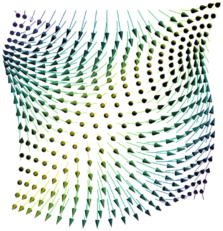
Refer to caption
(a) Noisy input
Refer to caption
(b) Result
Refer to caption
(c) Progression of the relative error
Refer to caption
(d) Progression of the isotropic 2superscript2\ell^{2}-TV cost
Figure 4: Runtime behavior of lRCPA and the proposed higher-order PD-RSSN method for an S2superscript𝑆2S^{2}-valued problem. The lRCPA method exhibits slow tail convergence as is typical for first-order methods. After few first-order pre-steps (shown in green), PD-RSSN superlinearly converges within 13 iterations to an optimal solution.
Case 2: =𝒫(3)𝒫3\mathcal{M}=\mathcal{P}(3)

Again we solved the isotropically regularized 2superscript2\ell^{2}-TV problem with α=0.5𝛼0.5\alpha=0.5. We set choose mi,j:=Iassignsubscript𝑚𝑖𝑗𝐼m_{i,j}:=I for all i,j=1,,10formulae-sequence𝑖𝑗110i,j=1,\ldots,10, so that n𝑛n is the zero vector in 𝒯m𝒫(3)10×10×2subscript𝒯𝑚𝒫superscript310102\mathcal{T}_{m}\mathcal{P}(3)^{10\times 10\times 2}. We initialized both PD-RSSN and lRCPA with σ=τ=0.4𝜎𝜏0.4\sigma=\tau=0.4. For lRCPA we used γ=0.2𝛾0.2\gamma=0.2 to control the primal and dual step size.

The pre-steps took 9.718 seconds. The resulting runtimes are shown in Table 3. The solutions returned by lRCPA and PD-RSSN at ϵrel=106subscriptitalic-ϵ𝑟𝑒𝑙superscript106\epsilon_{rel}=10^{-6} along with the error progress and the (isotropic) 2superscript2\ell^{2}-TV cost are shown in Fig. 5. We note that lRCPA effectively stalled before reaching the relative error of 106superscript10610^{-6} and was terminated after 2500 iterations.

𝒫(3)𝒫3\mathcal{P}(3) ϵrel=102subscriptitalic-ϵ𝑟𝑒𝑙superscript102\epsilon_{rel}=10^{-2} ϵrel=104subscriptitalic-ϵ𝑟𝑒𝑙superscript104\epsilon_{rel}=10^{-4} ϵrel=106subscriptitalic-ϵ𝑟𝑒𝑙superscript106\epsilon_{rel}=10^{-6}
Method Time (s) # Iterations Time (s) # Iterations Time (s) # Iterations
lRCPA 9.922 18 48.36 97 1213.327 \geq2500
PD-RSSN 237.062 5 380.047 8 556.328 12
Table 3: Runtimes and iteration count for lRCPA (comparison) and the proposed PD-RSSN method to converge to different accuracies ϵrelsubscriptitalic-ϵ𝑟𝑒𝑙\epsilon_{rel} for the two-dimensional 𝒫(3)𝒫3\mathcal{P}(3) problem. As in the positively-curved S2superscript𝑆2S^{2} case (Table 2), the proposed PD-RSSN algorithm outperforms lRCPA at higher accuracies on this negatively-curved manifold. lRCPA was terminated after 2500 iterations before achieving ϵrel=106subscriptitalic-ϵ𝑟𝑒𝑙superscript106\epsilon_{rel}=10^{-6}.

As for the S2superscript𝑆2S^{2} example, for higher accuracies PD-RSSN clearly outperforms lRCPA. The latter even seems unable to reach such high accuracies in reasonable time, which aligns with the fact that first-order methods generally show sublinear convergence. For PD-RSSN, we again observe superlinear convergence.
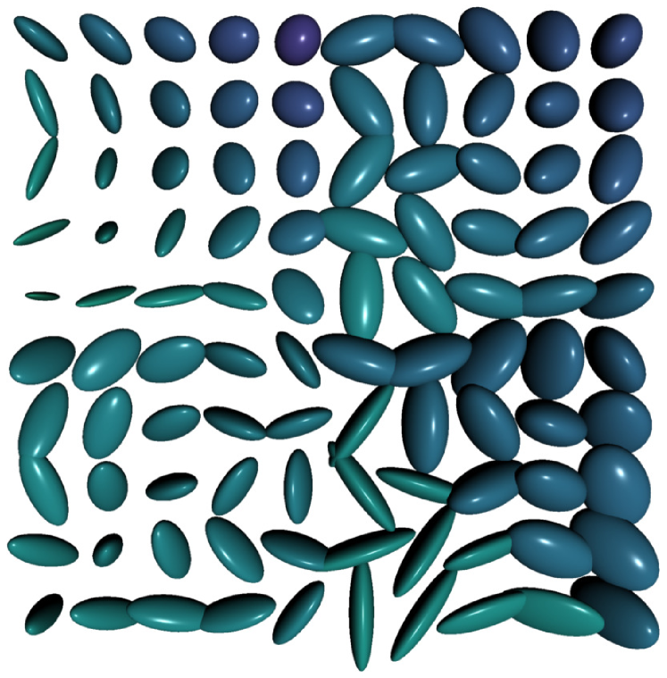
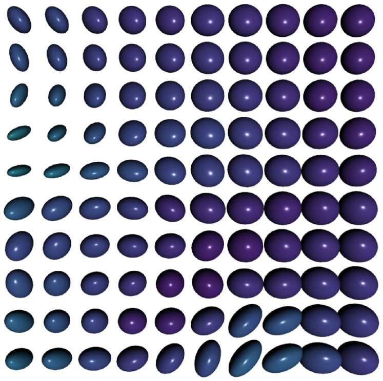
Refer to caption
(a) Noisy input
Refer to caption
(b) Result
Refer to caption
(c) Progression of the relative error
Refer to caption
(d) Progression of the isotropic 2superscript2\ell^{2}-TV cost
Figure 5: Results on the negatively-curved manifold 𝒫(3)𝒫3\mathcal{P}(3) (compare Fig. 4); first-order pre-steps are shown in green. The proposed PD-RSSN method superlinearly converges within 12 iterations after the pre-steps, while again lRCPA suffers from slow tail convergence.

6.3 Convergence Behavior of PD-RSSN for Different Problem Sizes

As computing a single Newton step scales quadratically at best, the convergence behavior of the proposed method for different problem sizes is important: Preferably, the number of required steps should not, or only very weakly, dependent on the problem size.

This type of convergence behavior is in general hard to measure precisely, because the problem will be slightly different at different scales. In order to get some intuition, we performed the following experiment using data from the previous one: For S2superscript𝑆2S^{2} we used the same N×N𝑁𝑁N\times N rotations image, and varied N=10,15,20,25,30.𝑁1015202530N=10,15,20,25,30. For 𝒫(3)𝒫3\mathcal{P}(3), we used the same artificial N×N𝑁𝑁N\times N image with N=4,7,10,13,16𝑁47101316N=4,7,10,13,16. We chose a tolerance of 106superscript10610^{-6} throughout the experiment. The remaining parameters and the initialization were identical to the ones in the previous experiment.

The results are shown in Tables 4 and 5. We see that larger problem sizes typically require more iterations, but the dependence seems to be weak: While the problem size varied by approximately an order of magnitude, the number of required PD-RSSN steps remained in the range of 8 to 15.

We would like to note briefly that the number of pre-steps needed for the largest problem size in the S2superscript𝑆2S^{2} example was considerably higher than for the other cases. Upon closer inspection, the convergence behavior in this case showed the typical oscillatory progression during the pre-steps as the lRCPA approach in Fig. 4(c) (blue line). However, for the smaller problem sizes, the pre-step stopping criterion of ϵrel=1/2subscriptitalic-ϵ𝑟𝑒𝑙12\epsilon_{rel}=1/2 was achieved within the first downwards cycle. For the largest problem, this was not the case, which greatly increases the number of first-order steps until the pre-step stopping criterion is met (compare again the blue line in Fig. 4(c)).

S2superscript𝑆2S^{2} Pre-steps PD-RSSN
Problem size Time (s) # Iterations Time (s) # Iterations
100 0.237 5 6.043 8
225 0.519 7 26.417 10
400 0.990 10 138.523 13
625 2.147 14 577.480 15
900 42.321 220 1109.928 11
Table 4: The effect of problem size on the amount of steps needed to converge to a solution with ϵrel=106subscriptitalic-ϵ𝑟𝑒𝑙superscript106\epsilon_{rel}=10^{-6} for the artificial problem on the S2superscript𝑆2S^{2} manifold. The PD-RSSN steps seem to increase slightly for the first four problems, but drops for the largest problem. However, for this problem more pre-steps were needed to reach the tolerance ϵrel=1/2subscriptitalic-ϵ𝑟𝑒𝑙12\epsilon_{rel}=1/2.
𝒫(3)𝒫3\mathcal{P}(3) Pre-steps PD-RSSN
Problem size Time (s) # Iterations Time (s) # Iterations
16 0.388 2 24.537 9
49 0.477 2 124.294 15
100 0.924 2 237.627 12
169 1.540 2 703.031 15
256 3.465 3 1602.052 15
Table 5: The effect of problem size on the amount of steps needed to converge to a solution with ϵrel=106subscriptitalic-ϵ𝑟𝑒𝑙superscript106\epsilon_{rel}=10^{-6} for the artificial problem on the 𝒫(3)𝒫3\mathcal{P}(3) manifold. Neither the pre-steps nor the PD-RSSN steps seem to be influenced much by the problem size.

6.4 Primal-Dual Inexact Riemannian Semi-smooth Newton (PD-IRSSN)

It is interesting to see if the convergence rates for the proposed inexact method in Algorithm 2 as predicted by Theorem 4.5 hold in practice. In particular, we expect linear convergence for constant relative residual ak=constantsuperscript𝑎𝑘constanta^{k}=\mathrm{constant} and superlinear convergence for ak0superscript𝑎𝑘0a^{k}\rightarrow 0. Given the similar behavior of the methods on positively and negatively curved manifolds in the previous experiments, we only consider the S2superscript𝑆2S^{2} manifold.

We used 2superscript2\ell^{2}-TV to denoise Bernoulli’s Lemniscate [9], which is a figure-8 on the 2-sphere. Note that this is once again a 1D problem. To this end, we sampled 128 S2superscript𝑆2S^{2}-valued points on the Lemniscate curve and distorted them with Gaussian noise with variance δ2=0.01superscript𝛿20.01\delta^{2}=0.01. We employed the 2superscript2\ell^{2}-TV model with α=0.5𝛼0.5\alpha=0.5 and m𝑚m set to the intersection point of the Lemniscate:

(118) mi:=12(1,0,1), for i=1,,128.formulae-sequenceassignsubscript𝑚𝑖12superscript101top for 𝑖1128m_{i}:=\frac{1}{\sqrt{2}}(1,0,1)^{\top},\quad\text{ for }i=1,\ldots,128.

We did not use dual regularization, i.e., β=0𝛽0\beta=0.

Again we warm-started PD-IRSSN using lRCPA pre-steps with σ=τ=0.35,𝜎𝜏0.35\sigma=\tau=0.35, γ=0.2𝛾0.2\gamma=0.2, and ϵrel=101subscriptitalic-ϵ𝑟𝑒𝑙superscript101\epsilon_{rel}=10^{-1}. In order to simulate inexact solution of the Newton steps, we defined three different progressions of the relative residual,

(119) a1k:=0,a2k:=15,a3k:=15k,formulae-sequenceassignsuperscriptsubscript𝑎1𝑘0formulae-sequenceassignsuperscriptsubscript𝑎2𝑘15assignsuperscriptsubscript𝑎3𝑘15𝑘a_{1}^{k}:=0,\qquad a_{2}^{k}:=\frac{1}{5},\qquad a_{3}^{k}:=\frac{1}{5k},

and randomly chose the corresponding absolute residual as

(120) rik:=aikX(pk,ξnk)(pk,ξnk)U(pk,ξnk), for i=1,2,3,formulae-sequenceassignsuperscriptsubscript𝑟𝑖𝑘superscriptsubscript𝑎𝑖𝑘subscriptnorm𝑋superscript𝑝𝑘superscriptsubscript𝜉𝑛𝑘superscript𝑝𝑘superscriptsubscript𝜉𝑛𝑘subscript𝑈superscript𝑝𝑘superscriptsubscript𝜉𝑛𝑘 for 𝑖123r_{i}^{k}:=a_{i}^{k}\|X(p^{k},\xi_{n}^{k})\|_{(p^{k},\xi_{n}^{k})}U_{(p^{k},\xi_{n}^{k})},\quad\text{ for }i=1,2,3,

where U(pk,ξnk)subscript𝑈superscript𝑝𝑘superscriptsubscript𝜉𝑛𝑘U_{(p^{k},\xi_{n}^{k})} is a tangent vector drawn from a normal distribution with unit covariance matrix. We then solved (to numerical precision) the modified inexact system for the step dksuperscript𝑑𝑘d^{k}:

(121) V(pk,ξnk)dk=X(pk,ξnk)+rik.subscript𝑉superscript𝑝𝑘superscriptsubscript𝜉𝑛𝑘superscript𝑑𝑘𝑋superscript𝑝𝑘superscriptsubscript𝜉𝑛𝑘superscriptsubscript𝑟𝑖𝑘V_{(p^{k},\xi_{n}^{k})}d^{k}=X(p^{k},\xi_{n}^{k})+r_{i}^{k}.

This allows to precisely control the residual and therefore simulate the behavior of PD-IRSSN at different accuracies.

From the error progression, we estimated a convergence rate q𝑞q by

(122) qk:=log(X(pk,ξnk)X(pk1,ξnk1))log(X(pk1,ξnk1)X(pk2,ξnk2)).assignsuperscript𝑞𝑘norm𝑋superscript𝑝𝑘superscriptsubscript𝜉𝑛𝑘norm𝑋superscript𝑝𝑘1superscriptsubscript𝜉𝑛𝑘1norm𝑋superscript𝑝𝑘1superscriptsubscript𝜉𝑛𝑘1norm𝑋superscript𝑝𝑘2superscriptsubscript𝜉𝑛𝑘2q^{k}:=\frac{\log\left(\frac{\|X(p^{k},\xi_{n}^{k})\|}{\|X(p^{k-1},\xi_{n}^{k-1})\|}\right)}{\log\left(\frac{\|X(p^{k-1},\xi_{n}^{k-1})\|}{\|X(p^{k-2},\xi_{n}^{k-2})\|}\right)}.

The results are shown in Fig. 6. As predicted by Theorem 4.5, for the exact method with zero residual a1subscript𝑎1a_{1} we obtain clear superlinear convergence. For constant relative residual a2subscript𝑎2a_{2}, convergence is clearly linear with rate q=1𝑞1q=1, and for decreasing relative residual a3subscript𝑎3a_{3}, convergence qualitatively appears superlinear – although hard to judge due to the rapid convergence – in agreement with the theorem.
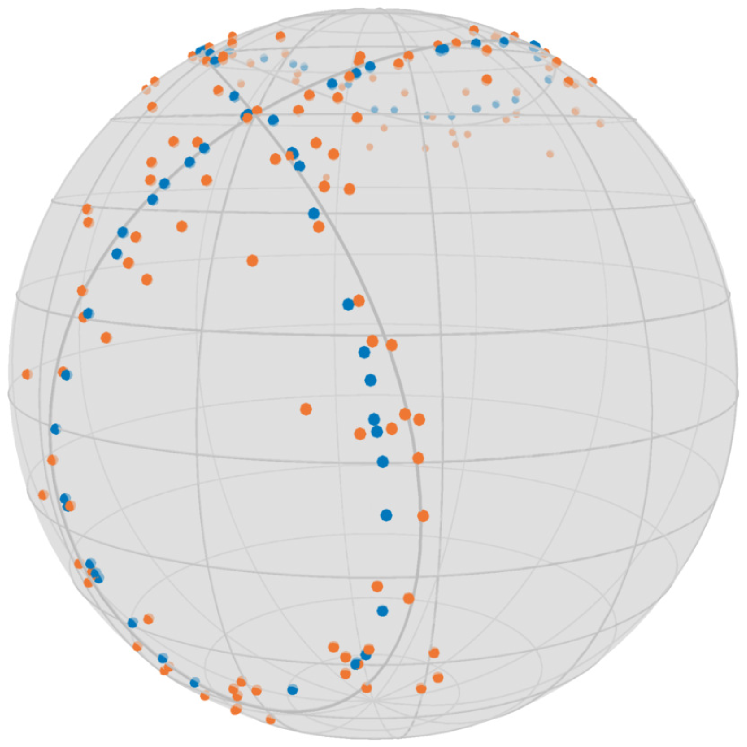
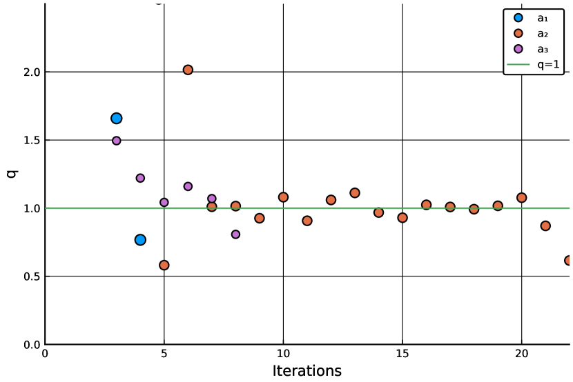
Refer to caption
(a) Bernoulli’s Lemniscate (grey), the noisy input (orange) and result (blue)
Refer to caption
(b) Estimated convergence rates after the pre-steps
Refer to caption
(c) Progression of the relative error of the lRCPA pre-steps (blue) and the three PD-IRSSN schemes
Refer to caption
(d) Progression of the 2superscript2\ell^{2}-TV cost of the lRCPA pre-steps (blue) and the three PD-IRSSN schemes
Figure 6: Convergence behavior of the Primal-Dual Inexact Riemannian Semi-smooth Newton method (PD-IRSSN) for recovering Bernoulli’s Lemniscate from noisy input data. As predicted by Theorem 4.5, exact PD-IRSSN, i.e., PD-RSSN, (a1subscript𝑎1a_{1}) and PD-IRSSN with progressively increasing accuracy (a3subscript𝑎3a_{3}) converge superlinearly. For constant relative accuracy (a2subscript𝑎2a_{2}), we still observe at least linear convergence.

7 Conclusions

In this work we have proposed the Primal-Dual Riemannian Semi-smooth Newton (PD-RSSN) method as a higher-order alternative for solving non-smooth variational problems on manifolds. Although the method is only locally convergent, it experimentally performs well on isotropic and anisotropic 1D and 2D 2superscript2\ell^{2}-TV problems. On both S2superscript𝑆2S^{2} and 𝒫(3)𝒫3\mathcal{P}(3), representing manifolds with positive and negative curvature, we observe superlinear convergence, which allows to generate high-accuracy solutions. In particular, PD-RSSN can be used to overcome the slow tail convergence that is a common bottleneck of first-order methods.

Moreover, we have proposed an inexact variant of RSSN (IRSSN) with provable local convergence rates. The theoretical results are supported by numerical experiments, in which we observe at least linear convergence in the inexact case, and superlinear convergence when accuracy is progressively increasing.

Acknowledgments

We would like to thank Ronny Bergmann for fruitful discussions regarding differential-geometric interpretations of earlier work and his Julia library Manopt.jl.

References

  • [1] T. E. Abrudan, J. Eriksson, and V. Koivunen, Steepest descent algorithms for optimization under unitary matrix constraint, IEEE Transactions on Signal Processing, 56 (2008), pp. 1134–1147, https://doi.org/10.1109/TSP.2007.908999.
  • [2] P.-A. Absil, C. G. Baker, and K. A. Gallivan, Trust-region methods on Riemannian manifolds, Foundations of Computational Mathematics, 7 (2007), pp. 303–330, https://doi.org/10.1007/s10208-005-0179-9.
  • [3] P.-A. Absil, R. Mahony, and R. Sepulchre, Optimization algorithms on matrix manifolds, Princeton University Press, 2009, https://doi.org/10.1515/9781400830244.
  • [4] B. L. Adams, S. I. Wright, and K. Kunze, Orientation imaging: the emergence of a new microscopy, Metallurgical Transactions A, 24 (1993), pp. 819–831, https://doi.org/10.1007/BF02656503.
  • [5] R. L. Adler, J.-P. Dedieu, J. Y. Margulies, M. Martens, and M. Shub, Newton’s method on Riemannian manifolds and a geometric model for the human spine, IMA Journal of Numerical Analysis, 22 (2002), pp. 359–390, https://doi.org/10.1093/imanum/22.3.359.
  • [6] B. Afsari, R. Tron, and R. Vidal, On the convergence of gradient descent for finding the Riemannian center of mass, SIAM Journal on Control and Optimization, 51 (2013), pp. 2230–2260, https://doi.org/10.1137/12086282X.
  • [7] D. Azagra and J. Ferrera, Proximal calculus on Riemannian manifolds, Mediterranean Journal of Mathematics, 2 (2005), pp. 437–450, https://doi.org/10.1007/s00009-005-0056-4.
  • [8] M. Bacák, Computing medians and means in Hadamard spaces, SIAM Journal on Optimization, 24 (2014), pp. 1542–1566, https://doi.org/10.1137/140953393.
  • [9] M. Bacák, R. Bergmann, G. Steidl, and A. Weinmann, A second order nonsmooth variational model for restoring manifold-valued images, SIAM Journal on Scientific Computing, 38 (2016), pp. A567–A597, https://doi.org/10.1137/15M101988X.
  • [10] S. Banert, Backward–backward splitting in Hadamard spaces, Journal of Mathematical Analysis and Applications, 414 (2014), pp. 656–665, https://doi.org/10.1016/j.jmaa.2014.01.054.
  • [11] P. J. Basser, J. Mattiello, and D. LeBihan, MR diffusion tensor spectroscopy and imaging, Biophysical journal, 66 (1994), pp. 259–267, https://doi.org/10.1016/S0006-3495(94)80775-1.
  • [12] M. Baust, A. Weinmann, M. Wieczorek, T. Lasser, M. Storath, and N. Navab, Combined tensor fitting and tv regularization in diffusion tensor imaging based on a Riemannian manifold approach, IEEE transactions on medical imaging, 35 (2016), pp. 1972–1989, https://doi.org/10.1109/TMI.2016.2528820.
  • [13] S. Becker and J. Fadili, A quasi-Newton proximal splitting method, in Advances in neural information processing systems, 2012, pp. 2618–2626, https://doi.org/10.5555/2999325.2999427.
  • [14] G. Bento, J. Neto, and P. Oliveira, Convergence of inexact descent methods for nonconvex optimization on Riemannian manifolds, arXiv preprint arXiv:1103.4828, (2011), https://arxiv.org/abs/1103.4828.
  • [15] G. d. C. Bento, J. X. da Cruz Neto, and P. R. Oliveira, A new approach to the proximal point method: convergence on general Riemannian manifolds, Journal of Optimization Theory and Applications, 168 (2016), pp. 743–755, https://doi.org/10.1007/s10957-015-0861-2.
  • [16] R. Bergmann, Manopt.jl, Optimization on Manifolds in Julia, (2019), https://doi.org/https://doi.org/10.5281/zenodo.4590042.
  • [17] R. Bergmann, R. H. Chan, R. Hielscher, J. Persch, and S. Gabriele, Restoration of manifold-valued images by half-quadratic minimization, Inverse Problems & Imaging, 10 (2016), pp. 281–304, https://doi.org/10.3934/ipi.2016001.
  • [18] R. Bergmann, J. H. Fitschen, J. Persch, and G. Steidl, Infimal convolution coupling of first and second order differences on manifold-valued images, in International Conference on Scale Space and Variational Methods in Computer Vision, Springer, 2017, pp. 447–459, https://doi.org/10.1007/978-3-319-58771-4_36.
  • [19] R. Bergmann, J. H. Fitschen, J. Persch, and G. Steidl, Priors with coupled first and second order differences for manifold-valued image processing, Journal of mathematical imaging and vision, 60 (2018), pp. 1459–1481, https://doi.org/10.1007/s10851-018-0840-y.
  • [20] R. Bergmann, R. Herzog, M. S. Louzeiro, D. Tenbrinck, and J. Vidal-Núñez, Fenchel duality theory and a primal-dual algorithm on Riemannian manifolds, Foundations of Computational Mathematics, (2021), https://doi.org/10.1007/s10208-020-09486-5.
  • [21] R. Bergmann, F. Laus, G. Steidl, and A. Weinmann, Second order differences of cyclic data and applications in variational denoising, SIAM Journal on Imaging Sciences, 7 (2014), pp. 2916–2953, https://doi.org/10.1137/140969993.
  • [22] R. Bergmann, J. Persch, and G. Steidl, A parallel Douglas–Rachford algorithm for minimizing ROF-like functionals on images with values in symmetric Hadamard manifolds, SIAM Journal on Imaging Sciences, 9 (2016), pp. 901–937, https://doi.org/10.1137/15M1052858.
  • [23] R. Bergmann and D. Tenbrinck, A graph framework for manifold-valued data, SIAM Journal on Imaging Sciences, 11 (2018), pp. 325–360, https://doi.org/10.1137/17M1118567.
  • [24] R. Bergmann and A. Weinmann, Inpainting of cyclic data using first and second order differences, in International Workshop on Energy Minimization Methods in Computer Vision and Pattern Recognition, Springer, 2015, pp. 155–168.
  • [25] D. P. Bertsekas, Incremental proximal methods for large scale convex optimization, Mathematical programming, 129 (2011), p. 163, https://doi.org/10.1007/s10107-011-0472-0.
  • [26] J. Bolte, S. Sabach, and M. Teboulle, Proximal alternating linearized minimization for nonconvex and nonsmooth problems, Mathematical Programming, 146 (2014), pp. 459–494, https://doi.org/10.1007/s10107-013-0701-9.
  • [27] M. Bortoloti, T. Fernandes, O. Ferreira, and J. Yuan, Damped Newton’s method on Riemannian manifolds, arXiv preprint arXiv:1803.05126, (2018), https://arxiv.org/abs/1803.05126.
  • [28] K. Bredies, M. Holler, M. Storath, and A. Weinmann, Total generalized variation for manifold-valued data, SIAM Journal on Imaging Sciences, 11 (2018), pp. 1785–1848, https://doi.org/10.1137/17M1147597.
  • [29] R. H. Byrd, G. M. Chin, J. Nocedal, and F. Oztoprak, A family of second-order methods for convex 1superscript1\ell^{1}-regularized optimization, Mathematical Programming, 159 (2016), pp. 435–467, https://doi.org/10.1007/s10107-015-0965-3.
  • [30] R. H. Byrd, J. Nocedal, and F. Oztoprak, An inexact successive quadratic approximation method for l-1 regularized optimization, Mathematical Programming, 157 (2016), pp. 375–396, https://doi.org/10.1007/s10107-015-0941-y.
  • [31] M. P. d. Carmo, Riemannian geometry, Birkhäuser, 1992.
  • [32] R. Castro, G. Di Giorgi, and W. Sierra, Secant method on Riemannian manifolds, arXiv preprint arXiv:1712.02655, (2017), https://arxiv.org/abs/1712.02655.
  • [33] A. Chambolle and T. Pock, A first-order primal-dual algorithm for convex problems with applications to imaging, Journal of mathematical imaging and vision, 40 (2011), pp. 120–145, https://doi.org/10.1007/s10851-010-0251-1.
  • [34] T. F. Chan, S. H. Kang, and J. Shen, Total variation denoising and enhancement of color images based on the CB and HSV color models, Journal of Visual Communication and Image Representation, 12 (2001), pp. 422–435, https://doi.org/10.1006/jvci.2001.0491.
  • [35] C. Chefd’Hotel, D. Tschumperlé, R. Deriche, and O. Faugeras, Regularizing flows for constrained matrix-valued images, Journal of Mathematical Imaging and Vision, 20 (2004), pp. 147–162, https://doi.org/10.1023/B:JMIV.0000011920.58935.9c.
  • [36] D.-Q. Chen, Fixed point algorithm based on quasi-Newton method for convex minimization problem with application to image deblurring, 2014, https://arxiv.org/abs/1412.4438.
  • [37] S. Chen, S. Ma, A. Man-Cho So, and T. Zhang, Proximal gradient method for nonsmooth optimization over the Stiefel manifold, SIAM Journal on Optimization, 30 (2020), pp. 210–239, https://doi.org/10.1137/18M122457X.
  • [38] W. Chen, H. Ji, and Y. You, An augmented Lagrangian method for 1superscript1\ell^{1}-regularized optimization problems with orthogonality constraints, SIAM Journal on Scientific Computing, 38 (2016), pp. B570–B592, https://doi.org/10.1137/140988875.
  • [39] C. Clason and T. Valkonen, Introduction to nonsmooth analysis and optimization, arXiv preprint arXiv:2001.00216, (2020).
  • [40] P. L. Combettes and J.-C. Pesquet, A Douglas–Rachford splitting approach to nonsmooth convex variational signal recovery, IEEE Journal of Selected Topics in Signal Processing, 1 (2007), pp. 564–574, https://doi.org/10.1109/JSTSP.2007.910264.
  • [41] P. L. Combettes and V. R. Wajs, Signal recovery by proximal forward-backward splitting, Multiscale Modeling & Simulation, 4 (2005), pp. 1168–1200, https://doi.org/10.1137/050626090.
  • [42] P. Cook, Y. Bai, S. Nedjati-Gilani, K. Seunarine, M. Hall, G. Parker, and D. C. Alexander, Camino: open-source diffusion-MRI reconstruction and processing, in 14th scientific meeting of the international society for magnetic resonance in medicine, vol. 2759, Seattle WA, USA, 2006, p. 2759.
  • [43] D. Cremers and E. Strekalovskiy, Total cyclic variation and generalizations, Journal of mathematical imaging and vision, 47 (2013), pp. 258–277, https://doi.org/10.1007/s10851-012-0396-1.
  • [44] T. De Luca, F. Facchinei, and C. Kanzow, A semismooth equation approach to the solution of nonlinear complementarity problems, Mathematical programming, 75 (1996), pp. 407–439, https://doi.org/10.1007/BF02592192.
  • [45] F. R. de Oliveira and O. P. Ferreira, Newton method for finding a singularity of a special class of locally Lipschitz continuous vector fields on Riemannian manifolds, arXiv preprint arXiv:1810.11636, (2018), https://arxiv.org/abs/1810.11636.
  • [46] J.-P. Dedieu, P. Priouret, and G. Malajovich, Newton’s method on Riemannian manifolds: covariant alpha theory, IMA Journal of Numerical Analysis, 23 (2003), pp. 395–419, https://doi.org/10.1093/imanum/23.3.395.
  • [47] W. Diepeveen, Non-smooth higher-order optimization on manifolds, master’s thesis, 2020, https://www.mic.uni-luebeck.de/fileadmin/mic/publications/StudentProjects/MasterTheses/2020-Diepeveen_Willem_MA-Theses.pdf.
  • [48] D. L. Donoho, Compressed sensing, IEEE Transactions on information theory, 52 (2006), pp. 1289–1306, https://doi.org/10.1109/TIT.2006.871582.
  • [49] A. Edelman, T. A. Arias, and S. T. Smith, The geometry of algorithms with orthogonality constraints, SIAM journal on Matrix Analysis and Applications, 20 (1998), pp. 303–353, https://doi.org/10.1137/S0895479895290954.
  • [50] E. Esser, X. Zhang, and T. F. Chan, A general framework for a class of first order primal-dual algorithms for convex optimization in imaging science, SIAM Journal on Imaging Sciences, 3 (2010), pp. 1015–1046, https://doi.org/10.1137/09076934X.
  • [51] F. Facchinei, A. Fischer, and C. Kanzow, Inexact Newton methods for semismooth equations with applications to variational inequality problems, in Nonlinear Optimization and Applications, Springer, 1996, pp. 125–139.
  • [52] F. Facchinei and J.-S. Pang, Finite-dimensional variational inequalities and complementarity problems, Springer Science & Business Media, 2007.
  • [53] O. Ferreira and P. Oliveira, Subgradient algorithm on Riemannian manifolds, Journal of Optimization Theory and Applications, 97 (1998), pp. 93–104, https://doi.org/10.1023/A:1022675100677.
  • [54] O. Ferreira and P. Oliveira, Proximal point algorithm on Riemannian manifolds, Optimization, 51 (2002), pp. 257–270, https://doi.org/10.1080/02331930290019413.
  • [55] P. T. Fletcher and S. Joshi, Riemannian geometry for the statistical analysis of diffusion tensor data, Signal Processing, 87 (2007), pp. 250–262, https://doi.org/10.1016/j.sigpro.2005.12.018.
  • [56] K. Fountoulakis, J. Gondzio, and P. Zhlobich, Matrix-free interior point method for compressed sensing problems, Mathematical Programming Computation, 6 (2014), pp. 1–31, https://doi.org/10.1007/s12532-013-0063-6.
  • [57] M. Giaquinta, G. Modica, and J. Souček, Variational problems for maps of bounded variation with values in s1superscript𝑠1s^{1}, Calculus of Variations and Partial Differential Equations, 1 (1993), pp. 87–121, https://doi.org/10.1007/BF02163266.
  • [58] M. Giaquinta and D. Mucci, The bv𝑏𝑣bv-energy of maps into a manifold: Relaxation and density results, Annali della Scuola Normale Superiore di Pisa-Classe di Scienze, 5 (2006), pp. 483–548.
  • [59] M. Giaquinta and D. Mucci, Maps of bounded variation with values into a manifold: total variation and relaxed energy, Pure and Applied Mathematics Quarterly, 3 (2007), pp. 513–538, https://doi.org/10.4310/PAMQ.2007.v3.n2.a6.
  • [60] R. Griesse and D. A. Lorenz, A semismooth Newton method for Tikhonov functionals with sparsity constraints, Inverse Problems, 24 (2008), p. 035007, https://doi.org/10.1088/0266-5611/24/3/035007.
  • [61] P. Grohs and S. Hosseini, Nonsmooth trust region algorithms for locally Lipschitz functions on Riemannian manifolds, IMA Journal of Numerical Analysis, 36 (2016), pp. 1167–1192, https://doi.org/10.1093/imanum/drv043.
  • [62] P. Grohs and S. Hosseini, ε𝜀\varepsilon-subgradient algorithms for locally lipschitz functions on Riemannian manifolds, Advances in Computational Mathematics, 42 (2016), pp. 333–360, https://doi.org/10.1007/s10444-015-9426-z.
  • [63] P. Grohs and M. Sprecher, Total variation regularization by iteratively reweighted least squares on Hadamard spaces and the sphere, preprint, 39 (2014).
  • [64] P. Grohs and M. Sprecher, Total variation regularization on Riemannian manifolds by iteratively reweighted minimization, Information and Inference: A Journal of the IMA, 5 (2016), pp. 353–378, https://doi.org/10.1093/imaiai/iaw011.
  • [65] B. He, Y. You, and X. Yuan, On the convergence of primal-dual hybrid gradient algorithm, SIAM Journal on Imaging Sciences, 7 (2014), pp. 2526–2537, https://doi.org/10.1137/140963467.
  • [66] J. He, J. Wang, and J.-C. Yao, Convergence criteria of Newton’s method on Lie groups, Fixed Point Theory and Applications, 2013 (2013), p. 293, https://doi.org/10.1186/1687-1812-2013-293.
  • [67] M. Hintermüller, K. Ito, and K. Kunisch, The primal-dual active set strategy as a semismooth Newton method, SIAM Journal on Optimization, 13 (2002), pp. 865–888, https://doi.org/10.1137/s1052623401383558.
  • [68] S. Hosseini, Convergence of nonsmooth descent methods via Kurdyka-Lojasiewicz inequality on Riemannian manifolds, Hausdorff Center for Mathematics and Institute for Numerical Simulation, University of Bonn (2015,(INS Preprint No. 1523)), (2015).
  • [69] S. Hosseini, W. Huang, and R. Yousefpour, Line search algorithms for locally Lipschitz functions on Riemannian manifolds, SIAM Journal on Optimization, 28 (2018), pp. 596–619, https://doi.org/10.1137/16M1108145.
  • [70] S. Hosseini and M. Pouryayevali, Generalized gradients and characterization of epi-Lipschitz sets in Riemannian manifolds, Nonlinear Analysis: Theory, Methods & Applications, 74 (2011), pp. 3884–3895, https://doi.org/10.1016/j.na.2011.02.023.
  • [71] S. Hosseini and A. Uschmajew, A Riemannian gradient sampling algorithm for nonsmooth optimization on manifolds, SIAM Journal on Optimization, 27 (2017), pp. 173–189, https://doi.org/10.1137/16M1069298.
  • [72] B. A. Kakavandi and M. Amini, Duality and subdifferential for convex functions on complete CAT(0) metric spaces, Nonlinear Analysis: Theory, Methods & Applications, 73 (2010), pp. 3450–3455, https://doi.org/10.1016/j.na.2010.07.033.
  • [73] R. Kimmel and N. Sochen, Orientation diffusion or how to comb a porcupine, Journal of Visual Communication and Image Representation, 13 (2002), pp. 238–248, https://doi.org/10.1006/jvci.2001.0501.
  • [74] A. Kovnatsky, K. Glashoff, and M. M. Bronstein, MADMM: a generic algorithm for non-smooth optimization on manifolds, in European Conference on Computer Vision, Springer, 2016, pp. 680–696, https://doi.org/10.1007/978-3-319-46454-1_41.
  • [75] R. Lai and S. Osher, A splitting method for orthogonality constrained problems, Journal of Scientific Computing, 58 (2014), pp. 431–449, https://doi.org/10.1007/s10915-013-9740-x.
  • [76] F. Laus, M. Nikolova, J. Persch, and G. Steidl, A nonlocal denoising algorithm for manifold-valued images using second order statistics, SIAM Journal on Imaging Sciences, 10 (2017), pp. 416–448, https://doi.org/10.1137/16M1087114.
  • [77] J. D. Lee, Y. Sun, and M. A. Saunders, Proximal Newton-type methods for minimizing composite functions, SIAM Journal on Optimization, 24 (2014), pp. 1420–1443, https://doi.org/10.1137/130921428.
  • [78] J. M. Lee, Smooth manifolds, in Introduction to Smooth Manifolds, Springer, 2013, pp. 1–31, https://doi.org/10.1007/978-1-4419-9982-5.
  • [79] J. Lellmann, E. Strekalovskiy, S. Koetter, and D. Cremers, Total variation regularization for functions with values in a manifold, in Proceedings of the IEEE International Conference on Computer Vision, 2013, pp. 2944–2951, https://doi.org/10.1109/ICCV.2013.366.
  • [80] T. Li and D. Krupka, The geometry of tangent bundles: Canonical vector fields, Geometry, 2013 (2013).
  • [81] X. Li, D. Sun, and K.-C. Toh, A highly efficient semismooth Newton Augmented Lagrangian method for solving LASSO problems, SIAM Journal on Optimization, 28 (2018), pp. 433–458, https://doi.org/10.1137/16M1097572.
  • [82] D. G. Luenberger, The gradient projection method along geodesics, Management Science, 18 (1972), pp. 620–631, https://doi.org/10.1287/mnsc.18.11.620.
  • [83] J. Martínez and L. Qi, Inexact Newton methods for solving nonsmooth equations, Journal of Computational and Applied Mathematics, 60 (1995), pp. 127–145, https://doi.org/10.1016/0377-0427(94)00088-I.
  • [84] D. Massonnet and K. L. Feigl, Radar interferometry and its application to changes in the earth’s surface, Reviews of geophysics, 36 (1998), pp. 441–500, https://doi.org/10.1029/97RG03139.
  • [85] A. Milzarek and M. Ulbrich, A semismooth Newton method with multidimensional filter globalization for 1superscript1\ell^{1}-optimization, SIAM Journal on Optimization, 24 (2014), pp. 298–333, https://doi.org/10.1137/120892167.
  • [86] H. Pan, Z. Jing, M. Lei, R. Liu, B. Jin, and C. Zhang, A sparse proximal Newton splitting method for constrained image deblurring, Neurocomputing, 122 (2013), pp. 245–257, https://doi.org/10.1016/j.neucom.2013.06.027.
  • [87] P. Patrinos, L. Stella, and A. Bemporad, Forward-backward truncated Newton methods for convex composite optimization, arXiv preprint arXiv:1402.6655, (2014), https://arxiv.org/abs/1402.6655.
  • [88] X. Pennec, Intrinsic statistics on Riemannian manifolds: Basic tools for geometric measurements, Journal of Mathematical Imaging and Vision, 25 (2006), p. 127, https://doi.org/10.1007/s10851-006-6228-4.
  • [89] X. Pennec, P. Fillard, and N. Ayache, A Riemannian framework for tensor computing, International Journal of computer vision, 66 (2006), pp. 41–66, https://doi.org/10.1007/s11263-005-3222-z.
  • [90] J. Persch, Optimization Methods for manifold-valued Image Processing, Verlag Dr. Hut, 2018.
  • [91] T. Pock and A. Chambolle, Diagonal preconditioning for first order primal-dual algorithms in convex optimization, in 2011 International Conference on Computer Vision, IEEE, 2011, pp. 1762–1769, https://doi.org/10.1109/ICCV.2011.6126441.
  • [92] L. Qi and J. Sun, A nonsmooth version of Newton’s method, Mathematical programming, 58 (1993), pp. 353–367, https://doi.org/10.1007/BF01581275.
  • [93] R. T. Rockafellar and R. J.-B. Wets, Variational analysis, vol. 317, Springer Science & Business Media, 2009, https://doi.org/10.1007/978-3-642-02431-3.
  • [94] L. I. Rudin, S. Osher, and E. Fatemi, Nonlinear total variation based noise removal algorithms, Physica D: nonlinear phenomena, 60 (1992), pp. 259–268, https://doi.org/10.1016/0167-2789(92)90242-F.
  • [95] C. Rust, Semiglatte Optimierungsverfahren zweiter Ordnung in der Bildverarbeitung, master’s thesis, University of Lübeck, 2017.
  • [96] T. Sakai, Riemannian geometry, vol. 149, American Mathematical Soc., 1996.
  • [97] S. T. Smith, Optimization techniques on Riemannian manifolds, Fields institute communications, 3 (1994), pp. 113–135.
  • [98] M. Storath and A. Weinmann, Wavelet sparse regularization for manifold-valued data, arXiv preprint arXiv:1808.00505, (2018), https://arxiv.org/abs/1808.00505.
  • [99] M. Storath, A. Weinmann, and M. Unser, Exact algorithms for l1superscript𝑙1l^{1}-tv regularization of real-valued or circle-valued signals, SIAM Journal on Scientific Computing, 38 (2016), pp. A614–A630, https://doi.org/10.1137/15M101796X.
  • [100] E. Strekalovskiy and D. Cremers, Total variation for cyclic structures: Convex relaxation and efficient minimization, in CVPR 2011, IEEE, 2011, pp. 1905–1911, https://doi.org/10.1109/CVPR.2011.5995573.
  • [101] D. Sun and J. Han, Newton and Quasi-Newton methods for a class of nonsmooth equations and related problems, SIAM Journal on Optimization, 7 (1997), pp. 463–480, https://doi.org/10.1137/S1052623494274970.
  • [102] C. Udriste, Convex functions and optimization methods on Riemannian manifolds, vol. 297, Springer Science & Business Media, 1994.
  • [103] T. Valkonen, A primal–dual hybrid gradient method for nonlinear operators with applications to MRI, Inverse Problems, 30 (2014), p. 055012.
  • [104] T. Valkonen, K. Bredies, and F. Knoll, Total generalized variation in diffusion tensor imaging, SIAM Journal on Imaging Sciences, 6 (2013), pp. 487–525, https://doi.org/10.1137/120867172.
  • [105] T. Vogt, E. Strekalovskiy, D. Cremers, and J. Lellmann, Lifting methods for manifold-valued variational problems, arXiv preprint arXiv:1908.03776, (2019), https://arxiv.org/abs/1908.03776.
  • [106] Y. Wang, J. Yang, W. Yin, and Y. Zhang, A new alternating minimization algorithm for total variation image reconstruction, SIAM Journal on Imaging Sciences, 1 (2008), pp. 248–272, https://doi.org/10.1137/080724265.
  • [107] A. Weinmann, L. Demaret, and M. Storath, Total variation regularization for manifold-valued data, SIAM Journal on Imaging Sciences, 7 (2014), pp. 2226–2257, https://doi.org/10.1137/130951075.
  • [108] A. Weinmann, L. Demaret, and M. Storath, Mumford–Shah and Potts regularization for manifold-valued data, Journal of Mathematical Imaging and Vision, 55 (2016), pp. 428–445, https://doi.org/10.1007/s10851-015-0628-2.
  • [109] S. J. Wright, R. D. Nowak, and M. A. Figueiredo, Sparse reconstruction by separable approximation, IEEE Transactions on Signal Processing, 57 (2009), pp. 2479–2493, https://doi.org/10.1109/TSP.2009.2016892.
  • [110] X. Xiao, Y. Li, Z. Wen, and L. Zhang, A regularized semi-smooth Newton method with projection steps for composite convex programs, Journal of Scientific Computing, 76 (2018), pp. 364–389, https://doi.org/10.1007/s10915-017-0624-3.
  • [111] W. Yin, S. Osher, D. Goldfarb, and J. Darbon, Bregman iterative algorithms for 1superscript1\ell^{1}-minimization with applications to compressed sensing, SIAM Journal on Imaging sciences, 1 (2008), pp. 143–168, https://doi.org/10.1137/070703983.
  • [112] J. Yu, S. Vishwanathan, S. Günter, and N. N. Schraudolph, A quasi-Newton approach to nonsmooth convex optimization problems in machine learning, Journal of Machine Learning Research, 11 (2010), pp. 1145–1200, https://doi.org/10.1145/1390156.1390309.
  • [113] M.-C. Yue, Z. Zhou, and A. M.-C. So, A family of inexact SQA methods for non-smooth convex minimization with provable convergence guarantees based on the Luo–Tseng error bound property, Mathematical Programming, 174 (2019), pp. 327–358, https://doi.org/10.1007/s10107-018-1280-6.
  • [114] H. Zhu, X. Zhang, D. Chu, and L.-Z. Liao, Nonconvex and nonsmooth optimization with generalized orthogonality constraints: An approximate augmented Lagrangian method, Journal of Scientific Computing, 72 (2017), pp. 331–372, https://doi.org/10.1007/s10915-017-0359-1.