Strata-based Quantification of Distributional Uncertainty in Socio-Economic Indicators: A Comparative Study of Indian States

Abstract

This paper reports a comprehensive study of distributional uncertainty in a few socio-economic indicators across the various states of India over the years 2001-2011. We show that the DGB distribution, a typical rank order distribution, provide excellent fits to the district-wise empirical data for the population size, literacy rate (LR) and work participation rate (WPR) within every states in India, through its two distributional parameters. Moreover, taking resort to the entropy formulation of the DGB distribution, a proposed uncertainty percentage (UP) unveils the dynamics of the uncertainty of LR and WPR in all states of India. We have also commented on the changes in the estimated parameters and the UP values from the years 2001 to 2011. Additionally, a gender based analysis of the distribution of these important socio-economic variables within different states of India has also been discussed. Interestingly, it has been observed that, although the distributions of the numbers of literate and working people has a direct (linear) correspondence with that of the population size, the literacy and work-participation rates are distributed independently of the population distributions.

Keywords: Entropy; Rank Order Distribution; Population Distribution; Literacy Rate; Work Participation Rate.

I Introduction

Socio-economic development of our world is majorly driven by people and their governance. The habitable area of the world is divided into distinct units, namely countries or dependent territories, governed by independent administrative bodies of different nature. These countries are further subdivided (first tier division) into smaller units, sometimes called states or provinces, for the purpose of internal governance, management and better policy making. For the administrative purpose and the ease of working in a local manner, these states or provinces are further subdivided (second tier division) into more smaller strata called counties or districts. Although further subdivisions are seen in some countries, most large countries have major administrative divisions up to the second tier. For example, USA is divided into states (first-tier division) which, in turn, are divided into counties (second-tier division). China is divided into provinces and direct-controlled municipalities (first level), which are split into prefectures (second level), and prefectures are divided into counties (third level). India is divided into states (first tier) and subsequently in districts (second-tier). Although there is wide heterogeneity among the administrative units (states or districts) in a country, these local administrative units can be seen as socially constructed strata, which serve as spatial scenarios for social and economic processes lopez2008 . Such administrative divisions are often regions of a country that are granted a certain degree of autonomy and manage themselves through local governments. In a growing number of developing countries, there is an attempt to proliferate sub-national administrative divisions for decentralization of local governments grossman2014 such that the reorganization may yield economic benefit for the cities ma2005 . Even in the absence of large administrative and political reforms, administrative units are constantly being created, destroyed, merged or split, demonstrating the fact that the sub-divisional strata within the countries undergo evolution.

The population distribution that does not distribute randomly eeckhout2004 ; kgbb ; ag2019 over different regions of a country is one of the key factors of the high degree of diversity and complexity christenson1980 of the internal regional administration of various countries and territories. In this context, the study and understanding of the geographical distribution of the population within a given country or region becomes relevant, as it is a necessary step for the development of theories that could accurately describe the evolution of human agglomerations batty2008 ; battym2013 . However, almost all studies regarding population distribution focus on city populations (see, for instance, kgbb ; ag2019 ; soo2005 ; makse2008 ; holmes2010 ; jia2010 ; rybski2011 ; douady2011 ; masucci2013 ), whereas the literature regarding the population distribution in administrative divisions is scarce mansilla2009 ; betten2013 .

Moreover, there are studies predicting strong correlation of the population of any city with many of the characterizing features of the inhabitants of the corresponding city: mean income, number of registered patents per capita, criminality rates, land value and rent prices christenson1980 ; batty2008 ; ag2019 . In this respect, it is important to study the correlations of various socio-economic variables with the population distribution of the smaller strata of a country. In particular, to frame better policies for the whole country as well as for these subdivisions, it is necessary to understand, in detail, the distribution and associated uncertainty or inequalities of different socio-economic indicators within and between these strata along with their relations with the populations. These would then help us to classify different strata (subdivisions) within a country into similar groups in terms of the policy requirements for their developments where the groups are formed based on their underlying difference in terms of the socio-economic indicators. Is there any particular stratum within the country that requires special attention than the rest or all the strata are equal in terms of their socio-economic characteristics? In an attempt to answer such questions, in this paper, we will propose and discuss an innovative way of quantifying the distributional uncertainty of the socio-economic factors within different strata (first tier subdivisions) of a country based on their rank-size pattern across the second-tier subdivisions.

To study the uncertainty characteristics of a given socio-economic factor within a strata (first-tier subdivision) of a country, we first fit an appropriate distribution to the rank-size values of this factor across all second-tier subdivisions within the strata. The well known Zipf’s law, alternatively known as power law or Pareto distribution zipf has been successfully used to model such rank-size data on socio-economic factors in its upper range of values, but observed to fail in the lower end of the rank-size distribution lan2000 ; newman2005 . Very recently, a universal framework through rank-order distribution has been developed to successfully model a wide-range of rank-size data from various areas in arts and science Martinez-Mekler09 ; ag2019 ; Ausloos/Cerqueti:2016 ; Alvarez-Martinez/etc:2011 ; Alvarez-Martinez/etc:2014 ; Oscar2017 ; Alvarez-Martinez/etc:2018 where a two-parameter discrete generalized beta (DGB) distribution is used instead of the one-parameter Pareto distribution. The DGB distribution is also shown to provide excellent fit to the rank-size data on various socio-economic parameters within a country and between different countries across the world ag2019 . Remarkably, this DGB distribution can indeed be obtained as an appropriate maximum-entropy distribution agmaxent and hence its entropy can be used to quantify the maximum uncertainty present in the empirical data distribution. We will follow this idea to develop an uncertainty measure based on the entropy value of the fitted DGB distribution to the empirical data on the given socio-economic factor across all second-tier subdivisions within the strata.

Our proposed uncertainty measure, which we refer to as the Uncertainty Percentage (UP), will indicate the distribution of the factor under study across different parts of the given strata; it will hence take the maximum value of 100% if the factor value (socio-economic condition) is the same across all parts of the strata, i.e., in all second-tier subdivision within it, indicating the equally distributed scenario (least inequality). On the other hand, our measure UP will take the minimum value of 0% if the inequality within the strata is extreme in that only one second-tier subdivision has a non-zero value of the factor under study (socio-economic condition is as desired in only one subdivision)! Any value of UP in between these two extrema will indicate how the targeted factor is distributed within different parts (subdivisions) of the strata with higher values indicating more uniformity (less inequality). Once this uncertainty measure is computed for all the strata within a country, they can be classified accordingly and can be used for their further in-depth comparisons. For example, the fitted DGB distribution of different socio-economic factor can be linked by established appropriate relationship between the corresponding parameter estimates which, along with our UP measure, provide further insights to characterize and classify different strata within a country for better policy making.

Further, by using our proposed idea, we will analyze uncertainty among the Indian states (first-tier strata) based on the census data for the years 2011 and 2001. In this paper, we focus on the basic three socio-economic entities, namely, population, literacy and working population. Like Population, education is a key element in any society that removes inequality from society, impacts the growth of employment and improves a country’s gross national product. On the other hand, the distributional inequality of unemployment rates (that is given by the size of the non-working population) plays an important role for structuring the economic development. These three factors, together controls, to a large extent, the development of the human resources in any society. For a vast and diverse country like India, which has so many states with very different cultures, it is very important to analyses the levels of literacy and employment across various states of India and union territories (UTs) and investigate their underlying distributional uncertainty or inequality. We would like to apply our proposed idea ag2019 ; agmaxent of fitting the DGB distribution to the empirical data on the said three factors for all the districts of each Indian states. In a subsequent analysis we measure the inequality across the second-tier subdivisions (districts) within a state via our proposed UP measure. The correlation of the distribution of literacy and employment rate within each state with its population distribution will be investigated by linking the parameters of the corresponding fitted DGB distributions. Additionally, to strengthen our proposition we have also performed a gender based analysis for all these socio-economic indicators. Finally, our temporal analysis provide an overall picture about the uncertainty or uniformity of the Indian states in terms of population, literacy and employment rates, their interrelations and changes from the year 2001 to 2011.

II Methodology

II.1 Modelling Empirical Data by DGB distribution

Let us consider a strata (e.g., state of a country) having $N$ second-tier subdivisions (e.g., districts). Suppose that a socio-economic factor under study (e.g., population, literacy, work participation rate, etc.) takes the value $x_{i}$ at the $i$-th subdivision for $i=1,\ldots,N$. We arrange these data in decreasing order of “importance” (size) and denote the rank of the $i$-th subdivision as $r_{i}$ for $i=1,\ldots,N$. We model these rank-size data $\{(r_{i},x_{i}):i=1,\ldots,N\}$ by the discrete generalized beta (DGB) distribution having probability mass function

$$f_{(a,b)}(r)=A\frac{(N+1-r)^{b}}{r^{a}},~{}~{}~{}~{}r=1,\ldots,N.$$ (1)

Here, in (1), $a,b$ are two real valued model parameters characterizing the underlying distributional structure and $A$ is the normalizing constant depending on $(a,b)$ ensuring that $\sum_{r=1}^{N}f_{(a,b)}(r)=1$. Note that, for the choice $b=0$, the probability mass function in (1) simplifies to that of the Pareto distribution. With different values of the two parameters $(a,b)$, the class of DGB distribution in (1) allows us to model a wide range of rank-size distributions having an inflection point ag2019 and can successfully model different types of socio-economic factors Martinez-Mekler09 ; ag2019 ; Ausloos/Cerqueti:2016 ; Alvarez-Martinez/etc:2011 ; Alvarez-Martinez/etc:2014 ; Oscar2017 ; Alvarez-Martinez/etc:2018

Given empirical rank-size data $\{(r_{i},x_{i}):i=1,\ldots,N\}$ of any socio-economic factor, we can fit the DGB distribution by estimating the model parameters $(a,b)$ by maximizing the likelihood of the observed data, given by

$$L(a,b)=\prod_{i=1}^{N}f_{(a,b)}(r_{i})^{{x}_{i}}=\prod_{i=1}^{N}\frac{(N+1-r_{i})^{b{x}_{i}}}{r_{i}^{a{x}_{i}}}A^{{x}_{i}}.$$ (2)

This maximum likelihood estimator is known to be asymptotically most efficient and also enjoys several other optimality properties. However, we need to use numerical optimization method to compute these estimates since the likelihood function in (2) does not posses an explicit form for its maximizer. Once we get the maximum likelihood estimator (MLE), $(\widehat{a},\widehat{b})$, of the model parameters $(a,b)$ we can then verify if the fitted DGB model is a good fit to the empirical data or not. For this purpose, we use the overall error in model fit, computed in terms of the Kolmogorov-Smirnov (KS) measure between the observed and the predicted cumulative rank-sizes. Denoting the predicted size of rank $r_{i}$ as $p_{i}=\left(\sum_{i=1}^{N}x_{i}\right)f_{(\widehat{a},\widehat{b})}(r_{i})$ for all $i=1,\ldots,N$, we define the KS goodness-of-fit measure as

$$KS=\max_{1\leq i\leq N}\left|\left(\sum_{j:r_{j}\leq r_{i}}p_{j}\right)-\left(\sum_{j:r_{j}\leq r_{i}}x_{j}\right)\right|.$$ (3)

The lower KS values indicate a better fitment of the model, i.e. the theoretically estimated fitted DGB distribution is very close to the empirically observed rank-sizes when the KS values are nearly vanishing. Zero KS value indicates perfect fit with no error for the observed data.

II.2 Quantification of Distributional Uncertainty

Once a DGB distribution is found to be well fitted for a socio-economic indicator within a strata, we propose to quantify the underlying distributional uncertainty by its entropy. Entropy is a widely used measure of disorder within any physical system. Although the idea of entropy was originally used in Thermodynamics long back, its major use in information science and allied disciplines were started after Shannon’s groundbreaking work shanon1 ; shanon2 on mathematical formulation of entropy in an information channel and Jayne’s Maximum entropy principle jaynes . Subsequently, the idea of entropy and maximum entropy distribution has been widely used to analyze and assess the uncertainty in several geographical or socioeconomic variables kapurbook

Here we also consider the DGB distribution, which is shown to be a maximum entropy rank-order distribution under appropriate utility constraints agmaxent For this DGB distribution having probability as given in (1), its Shannon entropy is given by

$$S_{N}(a,b) = -\sum_{r=1}^{N}f_{(a,b)}(r)\log f_{(a,b)}(r)=-\log A-A\sum_{r=1}^{N}\frac{(N+1-R)^{b}}{r^{a}}[b\log(N+1-r)-a\log r].$$ (4)

This entropy value $S(a,b)$ then gives the maximum amount of uncertainty (entropy) lying within the underlying rank-order distribution for the given utility constraints which are characterized by the model parameters $(a,b)$. Therefore, given the empirical rank-size data, once we obtain the estimated parameter value $(\widehat{a},\widehat{b})$, we can estimate the (maximum) amount of uncertainty in these data by the entropy of the fitted DGB distribution, i.e., by $\widehat{S}_{N}=S_{N}(\widehat{a},\widehat{b})$.

However, the estimated entropy value $\widehat{S}_{N}$ can vary from 0 to $\log(N)$ so it cannot be used to compare the uncertainty present in two distributions having different values of $N$. Since the strata may often have different number ($N$) of subdivisions, we cannot compare them by just using $\widehat{S}_{N}$ as a measure of uncertainty. Standardizing by the range, we then define our proposed uncertainty percentage (UP) measure as the proportion of entropy estimated from the fitted DGB distribution with respect to its maximum possible value, i.e.,

$$UP=\frac{S_{N}(\widehat{a},\widehat{b})}{\log N}\times 100\%.$$ (5)

Note that, clearly the UP measure takes the value 100% if $S_{N}(\widehat{a},\widehat{b})=\log(N)$ which holds if and only if $\widehat{a}=0=\widehat{b}$ indicating that the best-fitted rank-sizes are uniformly distributed over the subdivisions within the given strata; in other words, there is no inequality of the distribution of the targeted socio-economic indicator within different parts of the strata. On the other hand, the UP measure will be zero if $S_{N}(\widehat{a},\widehat{b})=0$ indicating the extremely dispersed distribution of the rank-sizes within the strata with only one subdivision having non-zero value of the targeted indicator. Therefore, the UP can be used to quantify the distributional uncertainty of the spread of the distribution of any socio-economic indicator within a strata measuring its $closeness$ to the optimum case of uniformity. Since the UP measure takes the value from 0 to 100%, irrespective of the value of $N$, it can then also be used to compare the uncertainty present within different strata as well as for different indicators.

II.3 Inter-relations between the distributions of two socio-economic variables

In any human agglomeration unit, most of the socio-economic indicators are highly correlated with each other. In particular, we have noted that the population distribution has a huge impact on the distribution of various socio-economic factors that had been explored in the literature via regression within the power law structure. However, in this paper, we have used the alternative DGB rank-order distribution that is noted to yield better fitment of the model to the empirical data. Being consistent with the fitted DGB distributions, we here propose to investigate the relationship between the distributions of any socio-economic indicator with the population distribution within different strata. To be more specific, our approach focus more on the inter-relation between the distributional structure and uncertainty of the socio-economic variables rather than the corresponding values of the indicators.

To investigate the relationship between the DGB distributions fitted to two variables within a strata, let us recall that the DGB distributions are characterized by its two model parameters $(a,b)$. Suppose that there are $T$ strata and, for the $j$-th stratum, the MLE of the parameters $(a,b)$ corresponding to the fitted population distribution is $(\widehat{a}_{Pj},\widehat{b}_{Pj})$ and the same for any targeted socio-economic indicator $Y$ (e.g., literacy or unemployment rate) is $(\widehat{a}_{Yj},\widehat{b}_{Yj})$, $j=1,\ldots,T$. Then to study the relationship between the best-fitted DGB distributions to the targeted indicator $Y$ and the population across the $T$ strata, it is enough to investigate the relationship between the corresponding parameters $(\widehat{a}_{Pj},\widehat{b}_{Pj})$ and $(\widehat{a}_{Yj},\widehat{b}_{Yj})$ for $j=1,\ldots,T$. The first attempt in this regard should be the examination of the (Pearson) bivariate correlations among these estimated parameters across strata. If this correlation is significantly higher (in absolute value), it indicates the linearity of their relationship which we may then further explore via appropriate multivariate regression models. The same can be studied using the UP values and also for any two socio-economic indicators (other than the population).

However, if there is no linear relationship between the fitted parameters or the UP values corresponding to two indicators, one should investigate their relation via appropriate non-parametric correlation coefficients (e.g., rank correlation). If this non-parametric correlation is found to be significant, then one may proceed for further analyses of their non-linear relationship using advanced statistical tools, which will not be considered in the present paper.

III Results: Understanding Uncertainty among Indian States

III.1 Data Description and Overall Statistics

We consider the data from Indian census which is conducted in every 10 years to capture a detailed picture of demographic, economic and social conditions of all persons in the country pertaining to that specific time. The raw census data for the years 2011 and 2001 are obtained from the Primary Census data and Digital library (www.censusindia.gov.in). Following the stratified administrative structure of India, we use the districts as smaller second-tier units within each state (first-tier strata) of India. According to the final census in 2011, there were 29 states and 7 UTs in India, which consist of the pool of strata in our analysis; for simplicity we will also refer the UTs as the State. It is important to note that some states, created at a later time, were not present in the earlier round of census (at the year 2001). The total number of districts within all the states of India was 640 and 593 in the years 2011 and 2001, respectively. Additionally, we will also use these census data separately for male and female populations for further gender-based uncertainty analysis in Section III.3.

Figure 1: Plot of LR and WPR for different states in the years 2001 and 2011, along with the corresponding linear fits. The black solid line represent the $y=x$ line (linear growth)

As mentioned earlier, in this paper, we focus on two important socio-economic factors, namely literacy and work participation rates, along with the population of any unit under consideration. For literacy computation, a person is defined to be literate if (s)he is aged more than 7 years and can both read and write with understanding in any language. On the other hand, a person who has worked in any economically productive activity for more than 6 months during the last one year preceding the data collection date is considered to be a worker (main or marginal). We analyze the data on the corresponding variables (in rate) defined as follows:

Literacy rate (LR) $$= \frac{\mbox{number of literate people in a district}}{\mbox{total population in that district}}\times 100,$$

Work Participation Rate (WPR) $$= \frac{\mbox{number of Workers in a district}}{\mbox{total Population in that district}}\times 100.$$

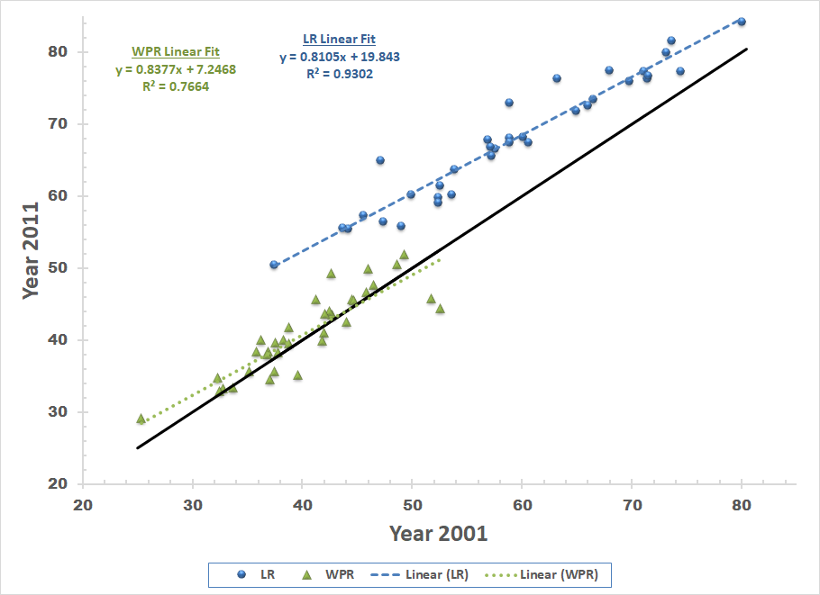
A comprehensive summary of state-wise population (P), LR and WPR statistics (in %) are reported in Supplementary Table S1 (Appendix A) for the years 2011 and 2001. It can easily be seen that the population of each state has increased over the years (linearly). To understand the changes in LR and WPR more clearly, we have plotted their values in the years 2001 versus in the year 2011 in Figure 1, along with the corresponding linear fit. According to 2011 census India has literacy rate (LR) around 84% to 50%, among which Kerala is highest and Bihar is lowest; but, the WPR for different states of India varies in between 35% to 50% only. Further, the LR has significantly increased in all the states whereas the changes in WPR is rather variables. Except for Mizoram and Kerala, all states has an increase of more than 5% in LR, with as many as 9 states having an increase of more than 10%. On the other hand, 10 states have no significant changes (only less than 1%) in the WPR. The UT of Dadra and Nagar Haveli has the highest increase in LR but maximum decrease in WPR. Nagaland is seen to have the highest increase of 6.64% in the WPR. Among larger states, Kerala, Himachal Pradesh, Assam, Jharkhand and Odisha has shown some amount of increase ($>2\%$) in WPR. Overall Tripura seems to have performed best considering both LR and WPR. On an average, there have been sublinear growths in both LR and WPR among the Indian states and UTs.

III.2 Modelling Population, Literacy and Work participation rates within each States

Fitting the DGB rank-order Distributions within each States:

We now discuss the results obtained by the application of the DGB distribution for different socioeconomic variables (Population, LR and WPR) for various states of India using the district-wise data. The states comprising of districts less than 5 are excluded from the analysis; this excludes 6 UTs (all except Delhi) and three states (Goa, Sikkim and Tripura). The values of the estimated parameters ($a,b$) and the goodness-of-fit measures (KS) for all three socioeconomic variables for different states, are reported in Table 1 for both the years 2011 and 2001. As expected (see ag2019 ; agmaxent ), the DGB distribution, with the two distributional parameters $\widehat{a}$ and $\widehat{b}$, provide excellent fits to the empirical data not only for Population size but also for LR and WPR with extremely small KS error.

Considering the distributional structures, for most states, both the parameters $\widehat{a}$ and $\widehat{b}$ tend to have positive values and are also nature-wise similar. However, there has been significant variations among the estimated parameter values across different states for all the variables, indicating differences in their distributions with the states (across districts). Particularly the UT of Delhi, the capital of India and one of the crowded states, has a negative $\widehat{a}$ value $-0.157$ and a positive $\widehat{b}$ value 1.387 for the distribution of populations. On the other hand, for modelling population, the not so much populated state Mizoram has a high positive value of $\widehat{a}$ (0.999) than any other states but a negative $\widehat{b}$ value. While considering the distribution of LR, most of the states fits to the positive values for both $\widehat{a}$ and $\widehat{b}$, except for Chandigarh, Delhi, Haryana, Mizoram which yield negative $\widehat{a}$ value and positive $\widehat{b}$ value. In 2011, Kerala, the state with 84 percent literate people, corresponds to $\widehat{a}$ and $\widehat{b}$ values of 0.018 and 0.035, respectively. West Bengal having 67.4 percent literate people gives $\widehat{a}$ and $\widehat{b}$ values 0.043 and 0.127. For the distribution of WPR as well, some states have negative $\widehat{a}$ value indicating their difference from the majority of the states. In general, disparity of LR among the states are more than that of WPR.

Table 1: The parameter estimates and the KS measures for for different states along with total numbers (N) of districts

		Population			LR			WPR
States	$N$	$\widehat{a}$	$\widehat{b}$	KS	$\widehat{a}$	$\widehat{b}$	KS	$\widehat{a}$	$\widehat{b}$	KS
Year 2011
India	640	0.252	0.872	0.005	0.063	0.133	0.004	0.082	0.109	0.006
Andhra Pradesh	23	0.124	0.171	0.007	0.074	0.050	0.001	-0.009	0.109	0.001
Arunachal Pradesh	16	0.074	0.825	0.020	0.069	0.125	0.002	0.122	0.033	0.003
Assam	27	0.265	0.307	0.011	0.076	0.070	0.002	0.060	0.071	0.006
Bihar	38	0.143	0.534	0.003	0.058	0.086	0.006	0.064	0.056	0.003
Chattishgarh	18	0.390	0.664	0.015	-0.022	0.285	0.005	0.044	0.059	0.002
Delhi	9	-0.157	1.387	0.026	0.015	0.033	0.001	0.101	0.022	0.006
Gujarat	26	0.383	0.454	0.020	0.021	0.112	0.003	0.112	0.011	0.003
Haryana	21	0.140	0.199	0.006	-0.014	0.150	0.004	0.020	0.105	0.002
Himachal Pradesh	12	0.306	0.748	0.035	0.009	0.076	0.001	0.059	0.119	0.005
Jammu Kashmir	22	0.368	0.487	0.011	0.141	0.049	0.003	0.175	0.046	0.004
Jharkhand	24	0.271	0.394	0.013	0.060	0.107	0.003	0.052	0.111	0.004
Karnataka	30	0.689	0.033	0.031	0.047	0.122	0.002	0.044	0.032	0.002
Kerala	14	0.056	0.592	0.011	0.018	0.035	0.002	0.074	0.107	0.006
Madyapradesh	50	0.197	0.293	0.005	0.016	0.159	0.005	0.048	0.098	0.001
Maharashtra	35	0.491	0.288	0.014	0.027	0.077	0.001	0.052	0.038	0.002
Manipur	9	0.126	0.623	0.030	0.038	0.103	0.003	0.054	0.059	0.001
Meghalayas	7	0.376	0.477	0.014	0.055	0.110	0.007	0.036	0.025	0.002
Mizoram	8	0.990	-0.119	0.020	-0.046	0.239	0.006	-0.008	0.184	0.003
Nagaland	11	0.241	0.563	0.012	0.050	0.171	0.004	0.107	0.109	0.005
Oddisha	30	0.239	0.488	0.007	0.027	0.230	0.005	0.035	0.167	0.008
Punjab	20	0.381	0.332	0.024	0.042	0.082	0.007	0.062	0.021	0.003
Rajasthan	33	0.367	0.211	0.012	0.062	0.066	0.003	0.063	0.049	0.001
TamilNadu	32	0.175	0.477	0.009	0.042	0.050	0.001	0.035	0.079	0.001
Uttarakhand	13	0.478	0.542	0.037	0.014	0.061	0.002	-0.001	0.191	0.006
Uttar Pradesh	71	0.147	0.394	0.018	0.030	0.116	0.002	0.079	0.026	0.003
West Bengal	19	0.255	0.364	0.006	0.043	0.127	0.002	0.051	0.024	0.001
Year 2001
India	593	0.236	0.808	0.007	0.077	0.192	0.004	0.074	0.123	0.005
Andhra Pradesh	23	0.125	0.148	0.009	0.103	0.077	0.003	-0.016	0.150	0.004
Arunachal Pradesh	13	0.130	0.490	0.011	0.103	0.131	0.005	0.082	0.080	0.002
Assam	23	0.252	0.357	0.012	0.077	0.099	0.004	0.146	0.041	0.005
Bihar	37	0.152	0.461	0.004	0.102	0.140	0.006	0.081	0.081	0.006
Chattishgarh	16	0.456	0.248	0.017	-0.038	0.322	0.009	0.037	0.081	0.004
Delhi	9	-0.094	1.163	0.021	0.003	0.051	0.001	0.027	0.077	0.003
Gujarat	25	0.360	0.419	0.018	0.019	0.168	0.003	0.051	0.065	0.002
Haryana	19	0.263	0.168	0.006	0.031	0.086	0.003	0.018	0.112	0.003
Himachal Pradesh	12	0.326	0.714	0.035	-0.002	0.109	0.002	0.114	0.033	0.003
Jammu Kashmir	14	0.166	0.766	0.019	0.182	0.077	0.005	0.166	0.083	0.017
Jharkhand	18	0.083	0.661	0.014	0.134	0.173	0.006	0.060	0.130	0.003
Karnataka	27	0.464	0.120	0.020	0.083	0.125	0.002	0.030	0.065	0.001
Kerala	14	0.021	0.596	0.012	0.021	0.048	0.002	0.085	0.104	0.005
Madyapradesh	45	0.104	0.357	0.004	0.030	0.163	0.004	0.061	0.090	0.002
Maharashtra	35	0.449	0.298	0.013	0.040	0.098	0.001	0.030	0.061	0.001
Manipur	9	0.350	0.409	0.029	0.098	0.077	0.003	0.024	0.075	0.002
Meghalaya	7	0.380	0.527	0.018	0.202	0.025	0.005	0.034	0.075	0.001
Mizoram	8	1.116	-0.305	0.009	-0.001	0.203	0.003	0.081	0.098	0.002
Nagaland	8	0.284	0.261	0.015	-0.005	0.353	0.006	0.044	0.178	0.008
Oddisha	30	0.246	0.481	0.008	0.024	0.334	0.005	0.057	0.179	0.010
Punjab	17	0.310	0.470	0.022	0.046	0.127	0.007	0.060	0.046	0.001
Rajasthan	32	0.331	0.225	0.012	0.080	0.086	0.003	0.066	0.051	0.003
TamilNadu	30	0.176	0.495	0.008	0.059	0.056	0.001	0.055	0.108	0.001
Uttarakhand	13	0.364	0.552	0.023	0.040	0.081	0.003	0.007	0.208	0.004
Uttar Pradesh	70	0.142	0.383	0.016	0.054	0.161	0.002	0.095	0.051	0.004
West Bengal	18	0.312	0.395	0.010	0.063	0.177	0.002	0.077	0.042	0.002

Next, if we compare the fitted distribution (their estimated parameters) for the two years 2011 and 2001, they changes more for the smaller states and the states having significantly change in district numbers. Among the states having mostly the same numbers of district in both 2001 and 2011, significant change in the values of the estimated parameters are observed for Bihar and meghalay while considering the LR distribution but the others remains mostly the same. However, the distribution of WPR has significant changes in more states including Assam, Delhi, Gujarat, Mizoram and Tamil Nadu.

Distributional Uncertainty Analysis:

We have revealed that the DGB distribution can completely characterize the population size, LR and WPR distributions through two $sensors$ or $drivers$ modelled by two parameters ($\widehat{a}$ , $\widehat{b}$). The predicted distribution fits very well with the observed rank-size data of all the districts of India as well as the data of the districts within the states. We now find the $entropy$ (S) values of all the considered distributions and take resort to the proposed entity $Uncertainty$ $Percentage$ (UP) by standardizing the $entropy$ $S$ values of the three variables of different Indian province. The resulting values of UP are plotted in Figure 2 for both the years 2011 and 2001.

(a) Year 2011

(b) Year 2001

Figure 2: Plots of UP for Populations, LR and WPR for different states of India in 2011 and 2001

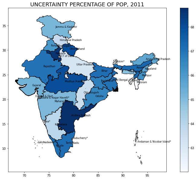
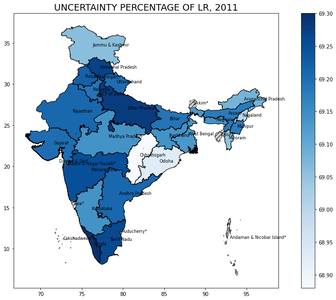
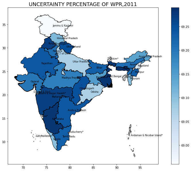
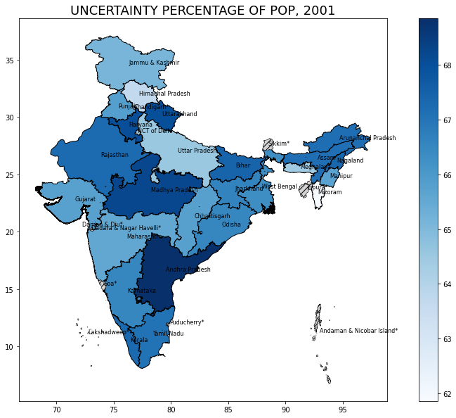
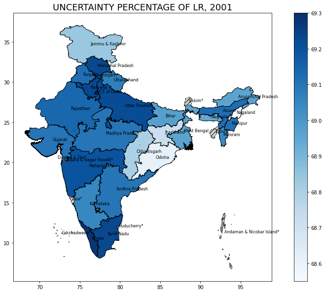
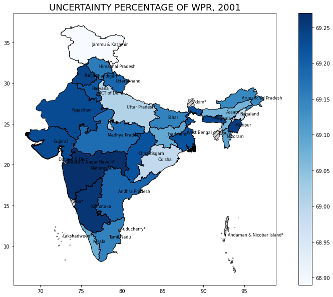
One can see from Figure 2 that the UP values changes mostly for the population and least for the WPR. So, there has been no significant changes in the distributional uncertainty of the work participation rates in all states on India. A little significant increase of 0.14% only is observed for the UP of WPR in Assam whereas it changes less that 0.1% in all other states. The changes in the UP values for LR is also less than 0.5% indicating no significant changes in the distributional uniformity of literacy rates in all the states in India. For the population, however, maximum increase (of 0.72%) in the UP values is observed in West Bengal indicating greater uniformity of its distribution within the states. On the other hand, in Karnataka and Chattisgarh, the UP values of population distribution decreases more than 2% indicating significant relocations of people within these states (mostly from rural areas to major cities).

In absolute term, Andhra Pradesh, Madhya Pradesh and Haryana has maximum UP values and hence more uniform population distribution, whereas those in Mizoram and Uttarakhand are more sparse. In terms of literacy rate, however, Delhi, Kerala and Uttarakhand are most evenly distributed states having highest UP values and Chhattisgarh and Odisha have most uneven distribution of LR (lowest UP values). Finally, Karnataka, West Bengal and Meghalaya have highest UP values for WPR indicating most equally distributed work-participation rates among their districts, whereas Jammu and Kashmir, Nagaland and Odisha have most uneven workforce within the states.

Relationship among the variables:

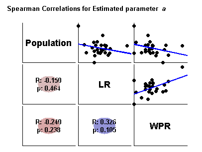
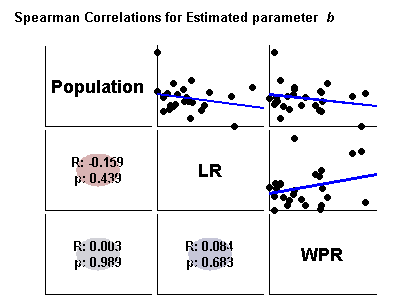
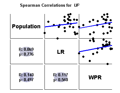
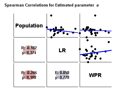
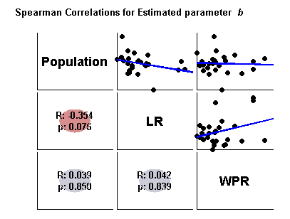
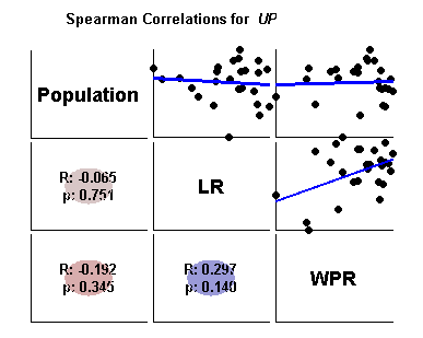
We have verified both the Pearson (linear) and the rank (non-parametric) correlation values between the variables population, LR and WPR in terms of the estimated parameters and the UP values for the years 2001 and 2011 separately; the rank correlations are illustrated in the supplementary Figure S1 (Appendix A). Interestingly, none of these correlations are significant at 95% level; the same is also observed for the Pearson correlations. This leads to the inference that the distributional uncertainty among these three indicators are mostly uncorrelated with each other across all the states of India. It is an important observation in contrast to the fact that the distribution of the numbers of literate and working persons in a population depends directly (linearly) on the corresponding population distribution.

III.3 Gender based analyses

The study on gender composition largely reflect the underlying social, economic and cultural patterns of the society in different ways. According to United Nation estimates, the world had 986 females against 1000 males in 2000. Interestingly the sheer weight of the population of the Asian countries, particularly China (944) and India (933) with low sex ratio contributes to the preponderance of males over females in world.

As per the Indian Census 2011, total population of India comprises of 62,37,24,248 males and 58,64,69,174 females with the sex ratio of 940 females per 1000 males. As per Census 2011, top five states/Union territories which have the highest sex ratio are Kerela (1,084) followed by Puducherry (1,038), Tamil Nadu (995), Andhra Pradesh (992) and Chhattisgarh (991). Five states which have the lowest sex ratio are Daman Diu (618), Dadra Nagar Haveli (775), Chandigarh (818), NCT of Delhi (866) and Andaman Nicobar Islands (878). The gender statistics revealed by Census India 2001, 532 million constituting 52 percent are males and 497 million constituting remaining 48 percent are females in the population. Eighteen states/Uts have recorded sex ratio above the national average of 933, while remaining seventeen falls below this. Chandigarh and Daman Diu occupy the bottom positions with less than 800 females per 1000 males. Though the Census has shown an increase in the sex ratio of total population from 933 in 2001 to 940 in 2011, it still requires further improvement for the balance of male -female ratio.

In any country, higher literacy rates improve development indicators consistently. In this respect, it is important to know the female percentage of the literate persons, as that may lead to better attainment of health and nutritional status, economic growth of community as a whole. The literacy rate of India in 2011 is 74.0 per cent. Literacy rate among females is 65.5 per cent whereas the literacy rate among males is 82.1 per cent showing a gap of 16.6 percent. If we see the data of 2001 census, the gap was 21.6 revealing development in this index .

Moreover, the male and female working population and work participation rate highlights the gender biased occupational distribution of a region. The Work Participation Rate (WPR), which is defined as the percentage of total workers to the total population, is 39.8 and 39.3 per cent as per the 2011 and 2001 census. While the WPR for males marginally increased from 51.6 percent to 51.9 percent during 1991-2001, for females it improved significantly from 22.7 to 25.7 during the corresponding period. Interestingly, this increase is mainly due to increase in proportion of marginal workers which registered significant increase from 3.4 percent to 8.7 percent. According to 2001 census, in the total population percentage of male non-workers and female non-workers are given by 48.1 percent and 74.3 percent respectively.

This gender based information of the census data inspired us to perform a gender-based analysis of the distribution of important socio-economic variables, such as population, literacy and work-participation rates of different states across India. According to our expectation, the analysis also revealed that both the male and female distributions fit very well with the DGBD. Besides, the DGB distribution fits very well with the male-female (sex) ratio of LR and WPR data for all the districts within the states of India with a very low value of KS (RO). For this purpose, we have computed the Sex-Ratio for the LR and WPR as follow:

Sex-Ratio of LR (SR-LR) $$= \frac{\mbox{number of female literate in a district}}{\mbox{number of male literate in that district}}\times 100,$$

Sex-Ratio of WPR (SR-WPR) $$= \frac{\mbox{number of female workers in a district}}{\mbox{number of male workers in that district}}\times 100.$$

(a) SR-LR

(b) SR-WPR

Figure 3: Plot of the UP values for the gender based SR-LR and SR-WPR for different states in the years 2011 vs. 2001, along with the corresponding linear fits. The black solid line represent the $y=x$ line (linear growth)

Table 2: The parameter estimates and the KS measures for different states along with total numbers (N) of districts and the UP values for Gender-based Analysis

		SR-LR				SR-WPR
States	$N$	$\widehat{a}$	$\widehat{b}$	KS	UP	$\widehat{a}$	$\widehat{b}$	KS	UP
Year 2011
Andhra Pradesh	23	0.079	0.027	0.003	69.24	0.010	0.292	0.004	68.77
Arunachal Pradesh	16	-0.003	0.211	0.002	69.03	0.146	0.200	0.008	68.56
Assam	27	0.027	0.018	0.001	69.30	0.125	0.255	0.022	68.48
Bihar	38	0.031	0.036	0.001	69.29	0.178	0.162	0.010	68.60
Chhattisgarh	18	0.017	0.079	0.001	69.26	0.028	0.157	0.006	69.10
Delhi	9	0.052	0.007	0.001	69.29	0.145	0.174	0.012	68.65
Gujarat	26	0.026	0.064	0.002	69.26	0.294	0.208	0.012	67.64
Haryana	21	-0.007	0.126	0.005	69.22	0.106	0.292	0.012	68.39
Himachal Pradesh	12	0.090	0.068	0.002	69.15	0.133	0.144	0.006	68.81
Jammu Kashmir	22	0.075	0.084	0.002	69.15	0.130	0.407	0.009	67.74
Jharkhand	24	0.051	0.044	0.001	69.26	0.062	0.332	0.007	68.44
Karnataka	30	0.064	0.046	0.001	69.24	0.065	0.162	0.003	69.01
Kerala	14	0.023	0.046	0.002	69.28	0.039	0.292	0.014	68.65
Madhya Pradesh	50	0.046	0.059	0.001	69.25	0.073	0.329	0.006	68.50
Maharashtra	35	0.049	0.026	0.000	69.28	0.027	0.294	0.003	68.74
Manipur	9	0.065	0.025	0.005	69.26	0.056	0.111	0.005	69.13
Meghalaya	7	0.153	0.015	0.001	69.11	0.257	-0.005	0.002	68.82
Mizoram	8	-0.014	0.163	0.003	69.16	0.114	0.035	0.004	69.16
Nagaland	11	0.038	0.037	0.002	69.28	-0.086	0.297	0.006	68.98
Odisha	30	0.046	0.062	0.002	69.24	0.023	0.702	0.014	67.03
Punjab	20	0.038	0.024	0.001	69.26	0.245	0.006	0.011	68.80
Rajasthan	33	0.034	0.081	0.001	69.24	0.086	0.141	0.003	69.01
Tamilnadu	32	0.047	0.030	0.001	69.28	0.117	0.192	0.007	68.75
Uttarakhand	13	0.067	0.068	0.002	69.19	-0.134	0.924	0.012	66.39
Uttar Pradesh	71	0.047	0.047	0.001	69.26	0.142	0.314	0.019	68.28
West Bengal	19	-0.009	0.100	0.004	69.25	0.180	0.197	0.008	68.41
Year 2001
Andhra Pradesh	23	0.117	0.045	0.003	69.13	-0.027	0.387	0.005	68.57
Arunachal Pradesh	13	0.038	0.203	0.006	68.95	0.101	0.231	0.003	68.63
Assam	23	0.026	0.037	0.003	69.29	0.193	0.314	0.014	67.81
Bihar	37	0.045	0.091	0.002	69.20	0.153	0.292	0.014	68.22
Chhattisgarh	16	0.089	0.073	0.005	69.14	0.056	0.116	0.008	69.13
Delhi	9	0.052	0.029	0.002	69.27	0.164	0.148	0.009	68.67
Gujarat	25	0.022	0.118	0.002	69.19	0.186	0.227	0.004	68.27
Haryana	19	0.063	0.036	0.001	69.25	0.041	0.445	0.007	68.02
Himachal Pradesh	12	0.134	0.082	0.005	69.00	0.166	0.054	0.002	68.97
Jammu Kashmir	14	0.112	0.081	0.003	69.07	0.140	0.446	0.012	67.37
Jharkhand	18	0.097	0.099	0.002	69.07	0.041	0.389	0.014	68.27
Karnataka	27	0.104	0.064	0.002	69.13	0.034	0.196	0.004	69.00
Kerala	14	0.022	0.047	0.001	69.28	0.037	0.374	0.006	68.32
Madhya Pradesh	45	0.055	0.098	0.002	69.18	0.070	0.280	0.006	68.66
Maharashtra	35	0.067	0.047	0.001	69.23	-0.022	0.381	0.012	68.61
Manipur	9	0.043	0.057	0.002	69.25	0.051	0.076	0.005	69.21
Meghalaya	7	0.142	0.063	0.003	69.03	-0.010	0.208	0.002	69.05
Mizoram	8	0.006	0.118	0.002	69.21	0.096	0.023	0.003	69.21
Nagaland	8	0.065	0.053	0.002	69.22	-0.172	0.480	0.020	68.61
Odisha	30	0.057	0.148	0.007	69.06	0.029	0.719	0.023	66.90
Punjab	17	0.038	0.037	0.001	69.28	0.172	0.170	0.005	68.56
Rajasthan	32	0.095	0.073	0.006	69.14	0.072	0.190	0.003	68.91
Tamilnadu	30	0.068	0.036	0.002	69.24	0.027	0.323	0.005	68.63
Uttarakhand	13	0.034	0.134	0.003	69.13	-0.185	1.054	0.020	69.13
Uttar Pradesh	70	0.061	0.101	0.002	69.17	0.098	0.578	0.022	67.45
West Bengal	18	-0.015	0.161	0.004	69.17	0.181	0.354	0.008	67.64

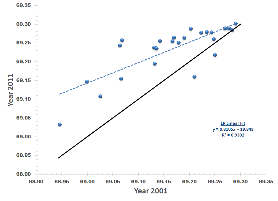
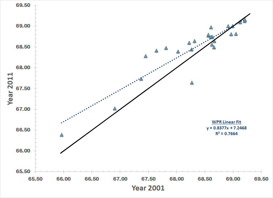
We apply our proposed analysis methodology for these two variables, depicting the gender based inequalities in LR and WPR, and the resulting parameter estimates and the UP values are presented in Table 2. For better understanding of the change in distributional uncertainty from the year 2001 to 2011, the UP values for both SR-LR and SR-WPR are also presented graphically in Figure 3 along with the linear fits. It can be seen that, on an average, there are sublinear growth of the distributional uncertainty (UP values) for both SR-LR and SR-WPR between years 2001 and 2011, indicating reduced gender-discriminations in literacy rate as well as in work-participation rate. For SR-LR, all states indeed have increased UP value in 2011, except for Haryana and Mizoram. The lowest UP value (most discrimination) is observed in Arunachal Pradesh for SR-LR and in Uttarakhand for SR-WPR. In general, the distributional uncertainty for SR-WPR remains mostly stable in the states having higher UP values, with slight uniform variations.

IV Conclusion

In this paper we have quantified the distributional uncertainty present in the various socio-economic indicators of all the Indian states, by studying the distribution of the districts within each individual states. The analysis is based on the DGB distribution, a typical rank-order distribution, which fits very well across many disciplines of Arts and Science. Despite the immense diversity of human settlements and extraordinary geographic variability, we have shown that all states obey DGB distribution not only for population size but also for other socioeconomic factors like literacy rate and work participation rate. The two model parameters of the distribution for different states construct a cluster. With the evolution of time there is no noted change in this cluster structure. Our primary analytical focus here is concerned with the entropy of the distribution. Although, the value of the entropy for a particular state for all factors are different, the Uncertainty Percentage (UP), a measure defined for the uncertainty, is almost the same for all the states of different size, culture and economic and social conditions. This is one of the most intriguing outcome of this analysis. The results also indicate that this value of UP is also nearly equal to the value of the UP when it is studied with all the districts across the states. Remarkably, the study for different years also indicate a similar result.

It is important to note that the proposed UP measure of distributional uncertainty is quite a general formulation which can further be applied to analyze the distributions of different important socio-economic variables of any country having stratified administrative structure. Beside such applications, it would also be important to investigate the detailed theoretical properties of the proposed UP measure as possible future research works.

Acknowledgment:
OM is thankful to Indian Statistical Institute, Kolkata, India for allowing her to work as a Visiting Student at the Physics and Applied Mathematics Unit of the Institute. SC thanks Science and Engineering Research Board (SERB), Government of India for financial support through Junior Research Fellowship (Grant No.CRG/2019/001461). The research of AG and BB is partially supported by a research grant (No. CRG/2019/001461) from the Science and Engineering Research Board (SERB), Government of India.

Appendix A Supplementary Tables and Figures

Table S1: Population (Pop), Literacy Rate (LR) and Work Participation Rate (WPR), along with the number of districts ($N$), for every states of India

	2011				2001
State	$N$	Pop	LR	WPR	$N$	Pop	LR	WPR
Andaman Nicobar (UT)	3	380581	77.32	40.08	2	356152	71.07	38.26
Andhra Pradesh	23	84580777	59.77	46.61	23	76210007	52.40	45.79
Arunachal Pradesh	16	1383727	55.36	42.47	13	1097968	44.15	43.98
Assam	27	31205576	61.46	38.36	23	26655528	52.58	35.78
Bihar	38	104099452	50.44	33.36	37	82998509	37.48	33.70
Chandigarh (UT)	1	1055450	76.31	38.29	1	900635	71.42	37.80
Chattisgarh	18	25545198	60.21	47.68	16	20833803	53.63	46.46
Dadra - Nagar Haveli (UT)	1	343709	64.95	45.73	1	220490	47.12	51.76
Daman - Diu (UT)	2	243247	77.45	49.86	2	158204	68.01	46.01
Delhi (UT)	9	16787941	75.87	33.28	9	13850507	69.78	32.82
Goa	2	1458545	79.91	39.58	2	1347668	73.13	38.80
Gujarat	26	60439692	67.99	40.98	25	50671017	58.87	41.95
Haryana	21	25351462	65.48	35.17	19	21144564	57.20	39.62
Himachal Pradesh	12	6864602	73.42	51.85	12	6077900	66.50	49.24
Jammu Kashmir	22	12541302	56.35	34.47	14	10143700	47.39	37.01
Jharkhand	24	32988134	55.56	39.71	18	26945829	43.71	37.52
Karnataka	30	61095297	66.53	45.62	27	52850562	57.59	44.53
Kerala	14	33406061	84.22	34.78	14	31841374	80.04	32.30
Lakshadweep (UT)	1	64473	81.51	29.09	1	60650	73.67	25.32
Madhya Pradesh	50	72626809	59.00	43.47	50	60348023	52.35	42.74
Maharashtra	35	112374333	72.57	43.99	35	96878627	66.03	42.50
Manipur	9	2855794	66.83	45.68	9	2293896	57.13	41.21
Meghalaya	7	2966889	60.16	39.96	7	2318822	49.93	41.84
Mizoram	8	1097206	77.30	44.36	8	888573	74.44	52.57
Nagaland	11	1978502	67.85	49.24	8	1990036	56.90	42.60
Odisha	30	41974218	63.71	41.79	30	36804660	53.90	38.79
Puducherry (UT)	4	1247953	76.71	35.66	4	974345	71.47	35.17
Punjab	20	27743338	67.43	35.67	17	24358999	60.58	37.47
Rajasthan	33	68548437	55.84	43.60	32	56507188	49.02	42.06
Sikkim	4	610577	72.87	50.47	4	540851	58.86	48.64
Tamilnadu	32	72147030	71.85	45.58	30	62405679	64.94	44.67
Tripura	4	3673917	76.34	40.00	4	3199203	63.21	36.25
Uttar Pradesh	71	199812341	57.25	32.94	70	166197921	45.56	32.48
Uttarakhand	13	10086292	68.22	38.39	13	8489349	60.14	36.92
West Bengal	19	91276115	67.42	38.08	18	80176197	58.87	36.77

(a) Year 2011

(b) Year 2011

(c) Year 2011

(d) Year 2001

(e) Year 2001

(f) Year 2001

Figure S1: Spearman Rank Correlation of the estimated parameters and UP values for Populations, LR and WPR in 2011 and 2001

References

- (1) Bettencourt L.M.A., West G.B., A Unified Theory of Urban Living, Nature 467 912.(2010)
- (2) Lopez-Pellicer F, Florczyk A, Lacasta J, Zarazaga-Soria F, Muro-Medrano P, Administrative units, an ontological perspective. In Proc. of the ER 2008Workshops (CMLSA, ECDM, FP-UML, M2AS, RIGiM, SeCoGIS, WISM) on Advances in Conceptual Modeling: Challenges and Opportunities, ER ’08, pp. 354–363. Berlin,Heidelberg: Springer.( 2008)
- (3) Luiz G.A. Alves, Haroldo V. Ribeiro, Ervin K. Lenzi, Renio S. Mendes Empirical analysis on the connection between power-law distributions and allometries for urban indicators, Physica A 409, 175 (2014)
- (4) Grossman G, Lewis J, Administrative unit proliferation. Am. Polit. Sci. Rev. 108, 196–217. (doi:10.1017/S0003055413000567) (2014)
- (5) Ma L, Urban administrative restructuring, changing scale relations and local economic development in China. Polit. Geogr. 24, 477–497. (doi:10.1016/j.polgeo.2004.10.005) (2005)
- (6) Eeckhout J, Gibrat’s Law for (all) cities. Am. Econ. Rev. 94, 1429–1451. (doi:10.1257/0002828043052303) (2004)
- (7) Gangopadhayay K and Basu B, The Morphology of Urban Agglomerations for Developing Countries: A Case Study with China Physica A 388 2682 (2009)
- (8) Ghosh A and Basu B, Universal City-size distributions through rank ordering, Physica A 528 121094 (2019)
- (9) Christenson J, Sachs C. The impact of government size and number of administrative units on the quality of public services. Adm. Sci. Q.25, 89–101. (doi:10.2307/2392228)(1980)
- (10) Human Behaviour and the principle of Least Effort (Addison-Wesley, Cambridge, MA, 1949)
- (11) LAN Amaral, Scala A, Barthlmy M and Stanley H. E., Classes of small-world networks Proc. Nat. Acad. Sci. 97 PNAS 11149 (2000)
- (12) Newman M. J., Power laws, Pareto distributions and Zipf’s law Contemporary Physics 46 323 (2005)
- (13) Batty M. The size, scale, and shape of cities,Science 319, 769–771. (doi:10.1126/science.1151419) (2008)
- (14) Batty M. , A theory of city size. Science 3402,1418–1419. (doi:10.1126/science.1239870) (2013)
- (15) Soo K. Zipf’s Law for cities: a cross-country investigation. Reg. Sci. Urban Econ. 35, 239–263. (doi:10.1016/j.regsciurbeco.2004.04.004) (2005)
- (16) Rozenfeld H, Rybski D, Jr JA, Batty M, Stanley H, Makse H. Laws of population growth. PNAS105, 18702–18707. (doi:10.1073/pnas.0807435105) (2008)
- (17) Holmes T, Lee S. Cities as six-by-six-mile squares: Zipfs Law? In Agglomeration economics (ed. E Glaeser), pp. 105–131. Chicago, IL: University of Chicago Press.(2010)
- (18) Jiang B, Jia T. Zipf’s law for all the natural cities in the United States: a geospatial perspective. Int. J. Geograph. Info. Sci. 25, 1269–1281. (doi:10.1080/ 13658816.2010.510801) (2010)
- (19) Rozenfeld H, Rybski D, Gabaix X, Makse H. The area and population of cities: new insights from a different perspective on cities. Am. Econ. Rev. 101, 2205–2225. (doi:10.3386/w15409) (2011)
- (20) Courtat T, Gloaguen C, Douady S. Mathematics and morphogenesis of cities: a geometrical approach. Phys. Rev. E 83, 036106. (doi:10.1103/PhysRevE 83.036106) (2011)
- (21) Masucci P, Stanilov K, Batty M , Limited urban growth: London’s street network dynamics since the 18th century. PLoS ONE 8, e69469. (doi:10.1371/ journal.pone.0069469) (2013)
- (22) Martínez-Mekler G, Martínez R, del Río MB, Mansilla R, Miramontes P, Cocho G. Universality of rank-ordering distributions in the arts and sciences. PLoS ONE 4, e4791. (doi:10.1371/ journal.pone.0004791) ( 2009)
- (23) Sahasranaman A and Bettencourt Luís M. A, Urban geography and scaling of contemporary Indian cities, J. R. Soc. Interface 16 20180758. http://dx.doi.org/10.1098/rsif.2018.0758 (2019)
- (24) Martínez-Mekler, G., R.A. Martínez, M.B. del Río, R. Mansilla, P. Miramontes, and G. Cocho, Universality of rank-ordering distributions in the arts and sciences. PLoS One, 4(3) e4791. (2009)
- (25) Ausloos M, and Cerqueti R, A universal rank-size law. PloS one, 11(11) e0166011. (2016)
- (26) Alvarez-Martinez, R., G. Martinez-Mekler, and G. Cocho, Order–disorder transition in conflicting dynamics leading to rank–frequency generalized beta distributions. Physica A: Statistical Mechanics and its Applications, 390 (1) 120 (2011)
- (27) Alvarez-Martinez, R., G. Cocho, R.F. Rodríguez, and G. Martínez-Mekler, Birth and death master equation for the evolution of complex networks. Physica A: Statistical Mechanics and its Applications, 402, (2014), 198
- (28) Fontanelli O., Miramontes P, Cocho G. and Li W, Population patterns in World’s administrative units, Royal Soc. Open Science, 4 170281 (2017)
- (29) Alvarez-Martinez R , Cocho G and Martinez-Mekler G, Rank ordered beta distributions of nonlinear map symbolic dynamics families with a first-order transition between dynamical regimes. Chaos: An Interdisciplinary Journal of Nonlinear Science, 28(7) 075515. (2018)
- (30) Ghosh A, Shreya P and Basu B, Maximum Entropy Framework for a Universal Rank Order distribution with Socio-economic Applications, 563, 125433 (2021)
- (31) Shannon, Claude E. . ”A Mathematical Theory of Communication”. Bell System Technical Journal. 27 (3): 379–423. doi:10.1002/j.1538-7305.1948.tb01338.x. hdl:10338.dmlcz/101429. (July 1948)
- (32) Shannon, Claude E. . ”A Mathematical Theory of Communication”. Bell System Technical Journal. 27 (4): 623–656. doi:10.1002/j.1538-7305.1948.tb00917.x. hdl:11858/00-001M-0000-002C-4317-B.(October 1948)
- (33) Jaynes E. T, Information Theory and Statistical Mechanics, Physical Review 106 (4) , 620 ( 1957)
- (34) Kapur, J. N. Maximum-entropy models in science and engineering, John Wiley and sons (1989).