Fair Sparse Regression with Clustering: An Invex Relaxation for a Combinatorial Problem

Abstract

In this paper, we study the problem of fair sparse regression on a biased dataset where bias depends upon a hidden binary attribute. The presence of a hidden attribute adds an extra layer of complexity to the problem by combining sparse regression and clustering with unknown binary labels. The corresponding optimization problem is combinatorial, but we propose a novel relaxation of it as an invex optimization problem. To the best of our knowledge, this is the first invex relaxation for a combinatorial problem. We show that the inclusion of the debiasing/fairness constraint in our model has no adverse effect on the performance. Rather, it enables the recovery of the hidden attribute. The support of our recovered regression parameter vector matches exactly with the true parameter vector. Moreover, we simultaneously solve the clustering problem by recovering the exact value of the hidden attribute for each sample. Our method uses carefully constructed primal dual witnesses to provide theoretical guarantees for the combinatorial problem. To that end, we show that the sample complexity of our method is logarithmic in terms of the dimension of the regression parameter vector.

1 Introduction

In modern times, machine learning algorithms are used in a wide variety of applications, many of which are decision making processes such as hiring [Hoffman et al.(2018)], predicting human behavior [Subrahmanian & Kumar(2017)], COMPAS (Correctional Offender Management Profiling for Alternative Sanctions) risk assessment [Brennan et al.(2009)], among others. These decisions have large impacts on society [Kleinberg et al.(2018)]. Consequently, researchers have shown interest in developing methods that can mitigate unfair decisions and avoid bias amplification. Several fair algorithms have been proposed for machine learning problems such as regression [Agarwal(2019), Berk(2017), Calders(2013)], classification [Agarwal et al.(2018), Donini et al.(2018), Dwork et al.(2012), Feldman et al.(2015), Hardt et al.(2016), Huang & Vishnoi(2019), Pedreshi et al.(2008), Zafar et al.(2019), Zemel et al.(2013)] and clustering [Backurs et al.(2019), Bera et al.(2019), Chen et al.(2019), Chierichetti et al.(2017), Huang et al.(2019)]. A common thread in the above literature is that performance is only viewed in terms of risks, e.g., misclassification rate, false positive rate, false negative rate, mean squared error.

In the literature, fairness is discussed in the context of discrimination based on membership to a particular group (e.g. race, religion, gender) which is considered a sensitive attribute. Fairness is generally modeled explicitly by adding a fairness constraint or implicitly by incorporating it in the model itself. There have been several notions of fairness studied in linear regression. [Berk(2017)] proposed notions of individual fairness and group fairness, and modeled them as penalty functions. [Calders(2013)] proposed the fairness notions of equal means and balanced residuals by modeling them as explicit constraints. [Agarwal(2019)], [Fitzsimons(2019)] and [Chzhen et al.(2020)] studied demographic parity. While [Agarwal(2019)], [Fitzsimons(2019)] modeled it as an explicit constraint, [Chzhen et al.(2020)] included it implicitly in their proposed model.

All the above work assume access to the sensitive attribute in the training samples and provide a framework which are inherently fair. Our work fundamentally differs from these work as we do not assume access to the sensitive attribute. Without knowing the sensitive attribute, it becomes difficult to ascertain bias, even for linear regression. In this work, we focus on identifying unfairly treated members/samples. This adds an extra layer of complexity to linear regression. We solve the linear regression problem while simultaneously solving a clustering problem where we identify two clusters – one which is positively biased and the other which is negatively biased. Table 1 shows a consolidated comparison of our work with the existing literature.

Once one identifies bias (positive or negative) for each sample, one could perform debiasing which would lead to the fairness notion of equal means [Calders(2013)] among the two groups (See Figure 1). It should be noted that identifying groups with positive or negative bias may not be same as identifying the sensitive attribute. The reason is that there may be multiple attributes that are highly correlated with the sensitive attribute. In such a situation, these correlated attributes can facilitate indirect discrimination even if the sensitive attribute is identified and removed. This is called the red-lining effect [Calders(2010)]. Our model avoids this by directly identifying biased groups.

Table 1: Comparison to prior work. Notation: $s$ is the number of non-zero entries in the regression parameter vector and $d$ is its dimension. The terms independent of $s$ and $d$ are not shown in the order notation.

Paper	Hidden sensitive attribute	Modeling type	Sample complexity
[Calders(2013), Agarwal(2019), Fitzsimons(2019)]	No	Explicit constraint	Not provided
[Berk(2017)]	No	Penalty function	Not provided
[Chzhen et al.(2020)]	No	Implicit	Not provided
Our paper	Yes	Implicit	$\Omega(s^{3}\log d)$

(a) Biased data without hidden sensitive attribute

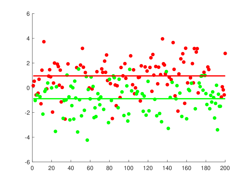
(b) Biased data after identifying hidden sensitive attribute

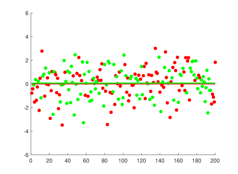
(c) Data after debiasing

Figure 1: Data before debiasing and after debiasing. Notice how means for two groups (shown as horizontal lines) become almost equal after debiasing.

While the standard algorithms solving the sparse/LASSO problem in this setting do provide an estimate of the regression parameter vector, they do not fit the model accurately as they fail to consider any fairness criteria in their formulations. It is natural then to think about including the hidden attribute in LASSO itself. However, this breaks the convexity of the loss function which makes the problem intractable by the standard LASSO algorithms. The resulting problem is a combinatorial version of sparse linear regression with added clustering according to the hidden attribute. In this work, we propose a novel technique to tackle the combinatorial LASSO problem with a hidden attribute and provide theoretical guarantees about the quality of the solution given a sufficient number of samples. Our method provably detects unfairness in the system. It should be noted that observing unfairness does not always imply that the designer of the system intended for such inequalities to arise. In such cases, our method acts as a check to detect and remove such unintended discrimination. While the current belief is that there is a trade-off between fairness and performance [Corbett-Davies et al.(2017), Kleinberg et al.(2017), Pleiss et al.(2017), Zliobaite(2015), Zhao & Gordon(2019)], our theoretical and experimental results show evidence on the contrary. Our theoretical results allow for a new understanding of fairness, as an “enabler” instead of as a “constraint”.

Contribution.

Broadly, we can categorize our contribution in the following points:

• Defining the problem: We formulate a novel combinatorial version of sparse linear regression which takes fairness/bias into the consideration. The addition of clustering comes at no extra cost in terms of the performance.

• Invex relaxation: Most of the current methods solve convex optimization problems as it makes the solution tractable. We propose a novel relaxation of the combinatorial problem and formally show that it is invex. To the best of our knowledge, this is the first invex relaxation for a combinatorial problem.

• Theoretical Guarantees: Our method can detect bias in the system. In particular, our method recovers the exact hidden attributes for each sample and thus provides an exact measure of bias between two different groups. Our method solves linear regression and clustering simultaneously with theoretical guarantees. To that end, we recover the true clusters (hidden attributes) and a regression parameter vector which is correct up to the sign of entries with respect to the true parameter vector. On a more technical side, we provide a primal-dual witness construction for our invex problem and provide theoretical guarantees for recovery. The sample complexity of our method varies logarithmically with respect to dimension of the regression parameter vector.

2 Notation and Problem Definition

In this section, we collect all the notations used throughout the paper. We also formally introduce our novel problem. We consider a problem where we have a binary hidden attribute, and where fairness depends upon the hidden attribute. Let $y\in$ be the response variable and $X\in^{d}$ be the observed attributes. Let $z^{*}\in\{-1,1\}$ be the hidden attribute and $\gamma\in_{>0}$ be the amount of bias due to the hidden attribute. The response $y$ is generated using the following mechanism:

$$\begin{split}y=X^{\intercal}w^{*}+\gamma z^{*}+e\end{split}$$ (1)

where $e$ is an independent noise term. For example, $y$ could represent the market salary of a new candidate, $X$ could represent the candidate’s skills and $z$ could represent the population group the candidate belongs to (e.g., majority or minority). While the group of the candidate is not public knowledge, a bias associated with the candidate’s group may be present in the underlying data. For our problem, we will assume that an estimate of the bias $\gamma\in_{>0}$ is available. In practice, even a rough estimate ($\pm 25\%$) of $\gamma$ also works well (See Appendix J).

Let $[d]$ denote the set $\{1,2,\cdots,d\}$. We assume $X\in^{d}$ to be a zero mean sub-Gaussian random vector [Hsu et al.(2012)] with covariance $\Sigma\in\mathbb{S}^{d}_{+}$, i.e., there exists a $\rho>0$, such that for all $\alpha\in^{d}$ the following holds: $\mathbb{E}(\exp(\alpha^{\intercal}X))\leq\exp(\frac{\|\alpha\|_{2}^{2}\rho^{2}}{2})$. By simply taking $\alpha_{i}=r$ and $\alpha_{k}=0,\forall k\neq i$, it follows that each entry of $X$ is sub-Gaussian with parameter $\rho$. In particular, we will assume that $\forall i\in[d]\,,\frac{X_{i}}{\sqrt{\Sigma_{ii}}}$ is a sub-Gaussian random variable with parameter $\sigma>0$. It follows trivially that $\max_{i\in[d]}\sqrt{\Sigma_{ii}}\sigma\leq\rho$. We will further assume that $e$ is zero mean independent sub-Gaussian noise with variance $\sigma_{e}$. We assume that as the number of samples increases, the noise in the model gently decreases. We model this by taking $\sigma_{e}=\frac{k}{\sqrt{\log n}}$ for some $k>0$. Our setting works with a variety of random variables as the class of sub-Gaussian random variable includes for instance Gaussian variables, any bounded random variable (e.g., Bernoulli, multinomial, uniform), any random variable with strictly log-concave density, and any finite mixture of sub-Gaussian variables. Notice that for the group with $z=+1$, $\mathbb{E}(y)=\gamma$ and for the group with $z=-1$, $\mathbb{E}(y)=-\gamma$. This means that after correctly identifying groups, one could perform debiasing by subtracting or adding $\gamma$ for $z=+1$ and $-1$ respectively. After debiasing, the expected value of both groups would match (and be equal to $0$). This complies with the notion of equal mean fairness proposed by [Calders(2013)].

The parameter vector $w^{*}\in^{d}$ is $s$-sparse, i.e., at most $s$ entries of $w^{*}$ are non-zero. We receive $n$ i.i.d. samples of $X\in^{d}$ and $y\in$ and collect them in $\mathbf{X}\in^{n\times d}$ and $\mathbf{y}\in^{n}$ respectively. Thus, in the finite-sample setting,

$$\begin{split}\mathbf{y}=\mathbf{X}w^{*}+\gamma\mathbf{z}^{*}+\mathbf{e}\,,\end{split}$$ (2)

where $\mathbf{z}^{*}\in\{-1,1\}^{n}$ and $\mathbf{e}\in^{n}$ both collect $n$ independent realizations of $z^{*}\in\{-1,1\}$ and $e\in$. Our goal is to recover $w^{*}$ and $\mathbf{z}^{*}$ using the samples $(\mathbf{X},\mathbf{y})$.

We denote a matrix $A\in^{p\times q}$ restricted to the columns and rows in $P\subseteq[p]$ and $Q\subseteq[q]$ respectively as $A_{PQ}$. Similarly, a vector $v\in^{p}$ restricted to entries in $P$ is denoted as $v_{P}$. We use ${\rm{eig}}_{i}(A)$ to denote the $i$-th eigenvalue ($1$st being the smallest) of matrix $A$. Similarly, ${\rm{eig}}_{\max}(A)$ denotes the maximum eigenvalue of matrix $A$. We use ${\rm{diag}}(A)$ to denote a vector containing the diagonal element of matrix $A$. By overriding the same notation, we use ${\rm{diag}}(v)$ to denote a diagonal matrix with its diagonal being the entries in vector $v$. We denote the inner product between two matrices $A$ and $B$ by $\langle A,B\rangle$, i.e., $\langle A,B\rangle={\rm{trace}}(A^{\intercal}B)$, where ${\rm{trace}}$ denotes the trace of a matrix. The notation $A\succeq B$ denotes that $A-B$ is a positive semidefinite matrix. Similarly, $A\succ B$ denotes that $A-B$ is a positive definite matrix. For vectors, $\|v\|_{p}$ denotes the $\ell_{p}$-vector norm of vector $v\in^{d}$, i.e., $\|v\|_{p}=(\sum_{i=1}^{d}|v_{i}|^{p})^{\frac{1}{p}}$. If $p=\infty$, then we define $\|v\|_{\infty}=\max_{i=1}^{d}|v_{i}|$. For matrices, $\|A\|_{p}$ denotes the induced $\ell_{p}$-matrix norm for matrix $A\in^{p\times q}$. In particular, $\|A\|_{2}$ denotes the spectral norm of $A$ and $\|A\|_{\infty}\triangleq\max_{i\in[p]}\sum_{j=1}^{q}|A_{ij}|$. A function $f(x)$ is of order $\Omega(g(x))$ and denoted by $f(x)=\Omega(g(x))$, if there exists a constant $C>0$ such that for big enough $x_{0}$, $f(x)\geq Cg(x),\forall x\geq x_{0}$. Similarly, a function $f(x)$ is of order $\mathcal{O}(g(x))$ and denoted by $f(x)=\mathcal{O}(g(x))$, if there exists a constant $C>0$ such that for big enough $x_{0}$, $f(x)\leq Cg(x),\forall x\geq x_{0}$. For brevity in our notations, we treat any quantity independent of $d,s$ and $n$ as constant. Detailed proofs for lemmas and theorems are available in the supplementary material.

3 Our New Optimization Problem and Invexity

In this section, we introduce our novel combinatorial problem and propose an invex relaxation. To the best of our knowledge, this is the first invex relaxation for a combinatorial problem. Without any information about the hidden attribute $\mathbf{z}^{*}$ in Equation (2), the following LASSO formulation could be incorrectly and unsuccessfully used to estimate the parameter $w^{*}$.

Definition 1 (Standard LASSO).

$$\begin{split}\begin{matrix}\min_{w}&\frac{1}{n}(\mathbf{X}w-\mathbf{y})^{\intercal}(\mathbf{X}w-\mathbf{y})+\lambda_{n}\|w\|_{1}\end{matrix}\end{split}$$ (3)

However, without including $\mathbf{z}^{*}$, standard LASSO does not provide accurate estimation of $w^{*}$ in Equation (2). We provide the following novel formulation of LASSO which fits our goals of estimating both $w^{*}$ and $z^{*}$:

Definition 2 (Combinatorial Fair LASSO).

$$\begin{split}\begin{matrix}\min_{w,\mathbf{z}}&\frac{1}{n}(\mathbf{X}w+\gamma\mathbf{z}-\mathbf{y})^{\intercal}(\mathbf{X}w+\gamma\mathbf{z}-\mathbf{y})+\lambda_{n}\|w\|_{1},&\text{\rm{such that }}\mathbf{z}_{i}\in\{-1,1\},\,\forall i\in[n],\end{matrix}\end{split}$$ (4)

where $\lambda_{n}>0$ is the regularization level which depends on $n$.

In its current form, optimization problem (4) is a non-convex mixed integer quadratic program (MIQP). Solving MIQP is NP-hard (See Appendix B). Next, we will provide a continuous but still non-convex relaxation of (4). For ease of notation, we define the following quantities:

$$\begin{split}&l(w)\triangleq\frac{1}{n}(\mathbf{X}w-\mathbf{y})^{\intercal}(\mathbf{X}w-\mathbf{y}),\;\mathbf{Z}\triangleq\begin{bmatrix}1&\mathbf{z}^{\intercal}\\ \mathbf{z}&\mathbf{z}\mathbf{z}^{\intercal}\end{bmatrix},\;\mathbf{M}(w)\triangleq\begin{bmatrix}l(w)&\frac{\gamma}{n}(\mathbf{X}w-\mathbf{y})^{\intercal}\\ \frac{\gamma}{n}(\mathbf{X}w-\mathbf{y})&\frac{\gamma^{2}}{n}\mathbf{I}_{n\times n}\end{bmatrix},\end{split}$$ (5)

where $\mathbf{I}$ is an $n\times n$ identity matrix. We provide the following invex relaxation to the optimization problem (4).

Definition 3 (Invex Fair LASSO).

$$\begin{split}\begin{matrix}\min_{w,\mathbf{Z}}&\langle\mathbf{M}(w),\mathbf{Z}\rangle+\lambda_{n}\|w\|_{1},\quad\text{\rm{such that}}&{\rm{diag}}(\mathbf{Z})=\mathbf{1},\;\mathbf{Z}\succeq\mathbf{0}_{n+1\times n+1}\end{matrix}\,.\end{split}$$ (6)

Note that optimization problem (6) is continuous and convex with respect to $w$ and $\mathbf{Z}$ separately but it is not jointly convex (See Appendix N for details). Specifically, for a fixed $w$, the matrix $\mathbf{M}(w)$ becomes a constant and problem (6) resembles a semidefinite program. For a fixed $\mathbf{Z}$, problem (6) resembles a standard LASSO. Unfortunately, problem (6) is not jointly convex on $w$ and $\mathbf{Z}$, and thus, it might still remain difficult to solve. Next, we will provide arguments that despite being non-convex, optimization problem (6) belongs to a particular class of non-convex functions namely “invex” functions. We define “invexity” of functions, as a generalization of convexity [Hanson(1981)].

Definition 4 (Invex function).

Let $\phi(t)$ be a function defined on a set $C$. Let $\eta$ be a vector valued function defined in $C\times C$ such that $\eta(t_{1},t_{2})^{\intercal}\nabla\phi(t_{2})$, is well defined $\forall t_{1},t_{2}\in C$. Then, $\phi(t)$ is a $\eta$-invex function if $\phi(t_{1})-\phi(t_{2})\geq\eta(t_{1},t_{2})^{\intercal}\nabla\phi(t_{2}),\,\forall t_{1},t_{2}\in C$.

Note that convex functions are $\eta$-invex for $\eta(t_{1},t_{2})=t_{1}-t_{2}$. [Hanson(1981)] showed that if the objective function and constraints are both $\eta$-invex with respect to same $\eta$ defined in $C\times C$, then Karush-Kuhn-Tucker (KKT) conditions are sufficient for optimality, while it is well-known that KKT conditions are necessary. [Ben-Israel & Mond(1986)] showed a function is invex if and only if each of its stationarity point is a global minimum.

In the next lemma, we show that the relaxed optimization problem (6) is indeed $\eta$-invex for a particular $\eta$ defined in $C\times C$ and a well defined set $C$. Before that, we will reformulate it into an equivalent optimization problem. Note that in the optimization problem (6), ${\rm{diag}}(\mathbf{Z})=\mathbf{1}$. Thus, $\langle\mathbf{I},\mathbf{Z}\rangle$ is a constant equal to $n+1$. Using this, we can rewrite the optimization problem as:

$$\begin{split}\begin{matrix}\min_{w,\mathbf{Z}}&\langle\mathbf{M}(w),\mathbf{Z}\rangle+\lambda_{n}\|w\|_{1}+\langle\mathbf{I},\mathbf{Z}\rangle,\quad\text{such that}&{\rm{diag}}(\mathbf{Z})=\mathbf{1},\;\mathbf{Z}\succeq\mathbf{0}_{n+1\times n+1}\end{matrix}\,,\end{split}$$ (7)

Let $C=\{(w,\mathbf{Z})\mid w\in^{d},{\rm{diag}}(\mathbf{Z})=\mathbf{1},\mathbf{Z}\succeq\mathbf{0}_{n+1\times n+1}\}$. We take $\mathbf{M}^{\prime}(w)=\mathbf{M}(w)+\mathbf{I}$ and the corresponding optimization problem becomes: $\min_{(w,\mathbf{Z})\in C}\langle\mathbf{M}^{\prime}(w),\mathbf{Z}\rangle+\lambda_{n}\|w\|_{1}$. We will show that $\forall(w,\mathbf{Z})\in C$, $\langle\mathbf{M}^{\prime}(w),\mathbf{Z}\rangle+\lambda_{n}\|w\|_{1}$ is an invex function. Note that by definition of the $\ell_{1}$-norm, $\|w\|_{1}=\sup_{\|a\|_{\infty}=1}\langle a,w\rangle$. Thus, it suffices to show that $\forall a\in^{d}$, $\langle\mathbf{M}^{\prime}(w),\mathbf{Z}\rangle$ and $\langle a,w\rangle$ are invex for the same $\eta(w,\bar{w},\mathbf{Z},\bar{\mathbf{Z}})$.

Lemma 1.

For $(w,\mathbf{Z})\in C$, the functions $f(w,\mathbf{Z})=\langle\mathbf{M}^{\prime}(w),\mathbf{Z}\rangle$ and $g(w,\mathbf{Z})=\langle a,w\rangle$ are $\eta$-invex for $\eta(w,\bar{w},\mathbf{Z},\bar{\mathbf{Z}})\triangleq\begin{bmatrix}w-\bar{w}\\ \mathbf{M}^{\prime}(\bar{w})^{-1}\mathbf{M}^{\prime}(w)(\mathbf{Z}-\bar{\mathbf{Z}})\end{bmatrix}$, where we abuse the vector/matrix notation for clarity of presentation, and avoid the vectorization of matrices.

Now that we have established that optimization problem (6) is invex, we are ready to discuss our main results in the next section.

4 Our Theoretical Analysis

In this section, we show that our Invex Fair Lasso formulation correctly recovers the hidden attributes and the regression parameter vector. More formally, we want to achieve the two goals by solving optimization problem (6) efficiently. First, we want to correctly and uniquely determine the hidden sensitive attribute for each data point, i.e., $\mathbf{z}^{*}\in\{-1,1\}^{n}$. Second, we want to recover regression parameter vector which is close to the true parameter vector $w^{*}\in^{d}$ in $\ell_{2}$-norm. Let $\tilde{w}$ and $\tilde{\mathbf{Z}}$ be the solution to optimization problem (6). Then, we will prove that $\tilde{w}$ and $w^{*}$ have the same support and $\tilde{\mathbf{z}}$ constructed from $\tilde{\mathbf{Z}}$ is exactly equal to $\mathbf{z}^{*}$. We define $\Delta\triangleq(\tilde{w}-w^{*})$.

4.1 KKT conditions

We start by writing the KKT conditions for optimization problem (6). Let $\mathbf{\mu}\in^{n+1}$ and $\Lambda\succeq\mathbf{0}_{n+1\times n+1}$ be the dual variables for optimization problem (6). For a fixed $\lambda_{n}$, the Lagrangian $L(w,\mathbf{Z};\mathbf{\mu},\Lambda)$ can be written as $L(w,\mathbf{Z};\mathbf{\mu},\Lambda)=\langle\mathbf{M}(w),\mathbf{Z}\rangle+\lambda_{n}\|w\|_{1}+\langle{\rm{diag}}(\mathbf{\mu}),\mathbf{Z}\rangle-\mathbf{1}^{\intercal}\mathbf{\mu}-\langle\Lambda,\mathbf{Z}\rangle$. Using this Lagrangian, the KKT conditions at the optimum can be written as:

1. Stationarity conditions:

   $$\begin{split}\frac{\partial{\langle\mathbf{M}(w),\mathbf{Z}\rangle}}{\partial{w}}+\lambda_{n}\mathbf{g}=\mathbf{0}_{d\times 1},\end{split}$$ (8)

   where $\mathbf{g}$ is an element of the subgradient set of $\|w\|_{1}$, i.e., $\mathbf{g}\in\frac{\partial{\|w\|_{1}}}{\partial{w}}$ and $\|\mathbf{g}\|_{\infty}\leq 1$.

   $$\begin{split}\mathbf{M}(w)+{\rm{diag}}(\mathbf{\mu})-\Lambda=\mathbf{0}_{n+1\times n+1}\end{split}$$ (9)

2. Complementary Slackness condition:

   $$\begin{split}\langle\Lambda,\mathbf{Z}\rangle=0\end{split}$$ (10)

3. Dual Feasibility condition:

   $$\begin{split}\Lambda\succeq\mathbf{0}_{n+1\times n+1}\end{split}$$ (11)

4. Primal Feasibility conditions:

   $$\begin{split}w\in^{d},\;{\rm{diag}}(\mathbf{Z})=\mathbf{1},\;\mathbf{Z}\succeq\mathbf{0}_{n+1\times n+1}\end{split}$$ (12)

Next, we will provide a setting for primal and dual variables which satisfies all the KKT conditions. But before that, we will describe a set of technical assumptions which will help us in our analysis.

4.2 Assumptions

Let $S$ denote the support of $w^{*}$, i.e., $S=\{i\,|\,w^{*}_{i}\neq 0,\,i\in[d]\}$. Similarly, we define the complement of support $S$ as $S^{c}=\{i\,|\,w^{*}_{i}=0,\,i\in[d]\}$. Let $|S|=s$ and $|S^{c}|=d-s$. For ease of notation, we define $\mathbf{H}\triangleq\mathbb{E}(XX^{\intercal})$ and $\hat{\mathbf{H}}\triangleq\frac{1}{n}\mathbf{X}^{\intercal}\mathbf{X}$. As the first assumption, we need the minimum eigenvalue of the population covariance matrix of $X$ restricted to rows and columns in $S$ to be greater than zero. Later, we will show that this assumption is needed to uniquely recover $w$ in the optimization problem (6).

Assumption 1 (Positive Definiteness of Hessian).

$\mathbf{H}_{SS}\succ\mathbf{0}_{s\times s}$ or equivalently ${\rm{eig}}_{\min}(\mathbf{H}_{SS})=C_{\min}>0$.

In practice, we only deal with finite samples and not populations. In the next lemma, we will show that with a sufficient number of samples, a condition similar to Assumption 1 holds with high probability in the finite-sample setting.

Lemma 2.

If Assumption 1 holds and $n=\Omega(\frac{s+\log d}{C_{\min}^{2}})$, then ${\rm{eig}}_{\min}(\hat{\mathbf{H}}_{SS})\geq\frac{C_{\min}}{2}$ with probability at least $1-\mathcal{O}(\frac{1}{d})$.

As the second assumption, we will need to ensure that the variates outside the support of $w^{*}$ do not exert lot of influence on the variates in the support of $w^{*}$. This sort of technical condition, known as the mutual incoherence condition, has been previously used in many problems related to regularized regression such as compressed sensing [Wainwright(2009)], Markov random fields [Ravikumar et al.(2010)], non-parametric regression [Ravikumar et al.(2007)], diffusion networks [Daneshmand et al.(2014)], among others. We formally present this technical condition in what follows.

Assumption 2 (Mutual Incoherence).

$\|\mathbf{H}_{S^{c}S}\mathbf{H}_{SS}^{-1}\|_{\infty}\leq 1-\alpha$ for some $\alpha\in(0,1]$.

Again, we will show that with a sufficient number of samples, a condition similar to Assumption 2 holds in the finite-sample setting with high probability.

Lemma 3.

If Assumption 2 holds and $n=\Omega(\frac{s^{3}(\log s+\log d)}{\tau(C_{\min},\alpha,\sigma,\Sigma)})$, then $\|\hat{\mathbf{H}}_{S^{c}S}\hat{\mathbf{H}}_{SS}^{-1}\|_{\infty}\leq 1-\frac{\alpha}{2}$ with probability at least $1-\mathcal{O}(\frac{1}{d})$ where $\tau(C_{\min},\alpha,\sigma,\Sigma)$ is a constant independent of $n,d$ and $s$.

In Appendix L, we experimentally show that Assumption 1 is easier to hold (i.e., $n\in\Omega(s+\log d)$) than Assumption 2 (i.e., $n\in\Omega(s^{3}\log d)$). Eventually, both assumptions hold as the number of samples increases.

4.3 Construction of Primal and Dual Witnesses

In this subsection, we will provide a construction of primal and dual variables which satisfies the KKT conditions for optimization problem (6). To that end, we provide our first main result.

Theorem 1 (Primal Dual Witness Construction).

If Assumptions 1 and 2 hold, $\lambda_{n}\geq\frac{128\rho k}{\alpha}\frac{\sqrt{\log d}}{n}$ and $n=\Omega(\frac{s^{3}\log d}{\tau_{0}(C_{\min},\alpha,\sigma,\Sigma,\rho,k,\gamma)})$, then the following setting of primal and dual variables

$$\begin{split}&\text{Primal Variables:}\quad\tilde{w}=(\tilde{w}_{S},\mathbf{0}_{d-s\times 1})\\ &\text{where, }\tilde{w}_{S}=\arg\min_{w_{S}}\frac{1}{n}(\mathbf{X}_{.S}w_{S}+\gamma\mathbf{z}^{*}-\mathbf{y})^{\intercal}(\mathbf{X}_{.S}w_{S}+\gamma\mathbf{z}^{*}-\mathbf{y})+\lambda_{n}\|w_{S}\|_{1}\\ &\mathbf{Z}=\mathbf{Z}^{*}\triangleq\begin{bmatrix}1&{\mathbf{z}^{*}}^{\intercal}\\ {\mathbf{z}^{*}}&{\mathbf{z}^{*}}{\mathbf{z}^{*}}^{\intercal}\end{bmatrix}\\ &\text{Dual Variables:}\quad\mathbf{\mu}=-{\rm{diag}}(M(\tilde{w})\mathbf{Z}^{*}),\quad\Lambda=M(\tilde{w})-{\rm{diag}}(M(\tilde{w})\mathbf{Z}^{*})\end{split}$$ (13)

satisfies all the KKT conditions for optimization problem (6) with probability at least $1-\mathcal{O}(\frac{1}{n})$, where $\tau_{0}(C_{\min},\alpha,\sigma,\Sigma,\rho,k,\gamma)$ is a constant independent of $s,d$ and $n$ and thus, the primal variables are a globally optimal solution for (6). Furthermore, the above solution is also unique.

Proof Sketch.

The main idea behind our proofs is to verify that the setting of primal and dual variables in Theorem 1 satisfies all the KKT conditions described in subsection 4.1. We do this by proving multiple lemmas in subsequent subsections. The outline of the proof is as follows:

• It can be trivially verified that the primal feasibility condition (12) holds. Similarly, the second stationarity condition (9) holds by construction of $\Lambda$.

• In subsection 4.4, we use Lemmas 4 and 11 to verify that the stationarity condition (8) holds.

• In subsection 4.5, we use Lemma 5 to verify the complementary slackness condition (10).

• In subsection 4.6, we show that the dual feasibility condition (11) is satisfied using results from Lemmas 6, 7, 8 and 12.

• Finally, in subsection 4.7, we show that our proposed solution is also unique.

4.4 Verifying the Stationarity Condition (8)

In this subsection, we will show that the setting of $\tilde{w}$ and $\mathbf{Z}^{*}$ satisfies the first stationarity condition (8) by proving the following lemma.

Lemma 4.

If Assumptions 1 and 2 hold, $\lambda_{n}\geq\frac{128\rho k}{\alpha}\frac{\sqrt{\log d}}{n}$ and $n=\Omega(\frac{s^{3}\log d}{\tau_{1}(C_{\min},\alpha,\sigma,\Sigma,\rho)})$, then the setting of $w$ and $\mathbf{Z}$ from equation (13) satisfies the stationarity condition (8) with probability at least $1-\mathcal{O}(\frac{1}{d})$, where $\tau_{1}(C_{\min},\alpha,\sigma,\Sigma,\rho)$ is a constant independent of $d,s$ or $n$.

4.5 Verifying the Complementary Slackness (10)

Next, we will show that the setting of $\Lambda$ and $\mathbf{Z}$ in (13) satisfies the complementary slackness condition (10). To this end, we will show the following:

Lemma 5.

Let $\Lambda$ be defined as in equation (13), then $\zeta^{*}\triangleq\begin{bmatrix}1\\ \mathbf{z}^{*}\end{bmatrix}$ is an eigenvector of $\Lambda$ corresponding to the eigenvalue $0$. Furthermore, $\langle\Lambda,\mathbf{Z}^{*}\rangle=0$.

Proof.

We will show that $\Lambda\zeta^{*}=\mathbf{0}_{n+1\times 1}$. Note that,

$$\begin{split}\Lambda=M(w)-{\rm{diag}}(M(w)\mathbf{Z}^{*})=\begin{bmatrix}-\frac{\gamma}{n}(Xw-y)^{T}\mathbf{z}^{*}&\frac{\gamma}{n}(Xw-y)^{T}\\ \frac{\gamma}{n}(Xw-y)&-{\rm{diag}}(\frac{\gamma}{n}(Xw-y){\mathbf{z}^{*}}^{T})\end{bmatrix}\end{split}$$

Multiplying the above matrix with $\zeta^{*}$ gives us $\mathbf{0}_{n+1\times 1}$. Now $\langle\Lambda,\mathbf{Z}^{*}\rangle={\rm{trace}}(\Lambda^{\intercal}\mathbf{Z}^{*})={\rm{trace}}(\Lambda\zeta^{*}{\zeta^{*}}^{\intercal})=0$ as $\Lambda\zeta^{*}=\mathbf{0}_{n+1\times 1}$. ∎

4.6 Verifying the Dual Feasibility (11)

We have already shown that $\Lambda$ has $0$ as one of its eigenvalues. To verify that it satisfies the dual feasibility condition (11), we show that second minimum eigenvalue of $\Lambda$ is greater than zero with high probability. At this point, it might not be clear why strict positivity is necessary, but this will be argued later in subsection 4.7. Now, note that:

$$\begin{split}&\mathbb{P}({\rm{eig}}_{2}(\Lambda)>0)\geq\mathbb{P}({\rm{eig}}_{2}(\Lambda)>0,\,\|\Delta\|_{2}\leq h(n))\geq\mathbb{P}({\rm{eig}}_{2}(\Lambda)>0|\|\Delta\|_{2}\leq h(n))\mathbb{P}(\|\Delta\|_{2}\leq h(n))\end{split}$$ (14)

where $h(n)$ is a function of $n$. We bound $\mathbb{P}({\rm{eig}}_{2}(\Lambda)>0)$ in two parts. First, we bound $\mathbb{P}({\rm{eig}}_{2}(\Lambda)>0)$ given that $\|\Delta\|_{2}\leq h(n)$ and then we bound the probability of $\|\Delta\|_{2}\leq h(n)$.

Lemma 6.

Given that $\|\Delta\|_{2}\leq h(n)$, the second minimum eigenvalue of $\Lambda$ as defined in equation (13) is strictly greater than $0$ with probability at least $1-\exp(-\frac{\gamma^{2}}{8(\rho^{2}h(n)^{2}+\sigma_{e}^{2})}+\log n)$.

Proof.

As the first step, we invoke Haynesworth’s inertia additivity formula [Haynsworth(1968)] to prove our claim. Let $R$ be a block matrix of the form $R=\begin{bmatrix}A&B\\ B^{\intercal}&C\end{bmatrix}$, then inertia of matrix $R$, denoted by ${\rm{In}}(R)$, is defined as the tuple $(\pi(R),\nu(R),\delta(R))$ where $\pi(R)$ is the number of positive eigenvalues, $\nu(R)$ is the number of negative eigenvalues and $\delta(R)$ is the number of zero eigenvalues of matrix $R$. Haynesworth’s inertia additivity formula is given as:

$$\begin{split}{\rm{In}}(R)={\rm{In}}(C)+{\rm{In}}(A-B^{\intercal}C^{-1}B)\end{split}$$ (15)

Note that,

$$\begin{split}&\Lambda=\mathbf{M}(w)-{\rm{diag}}(\mathbf{M}(w)\mathbf{Z}^{*})=\begin{bmatrix}-\frac{\gamma}{n}(\mathbf{X}w-\mathbf{y})^{\intercal}\mathbf{z}^{*}&\frac{\gamma}{n}(\mathbf{X}w-\mathbf{y})^{\intercal}\\ \frac{\gamma}{n}(\mathbf{X}w-\mathbf{y})&-{\rm{diag}}(\frac{\gamma}{n}(\mathbf{X}w-\mathbf{y}){\mathbf{z}^{*}}^{\intercal})\end{bmatrix}\end{split}$$

Then the following holds true by applying equation (15):

$$\begin{split}{\rm{In}}(\Lambda)=&{\rm{In}}(-{\rm{diag}}(\frac{\gamma}{n}(\mathbf{X}w-\mathbf{y}){\mathbf{z}^{*}}^{\intercal}))+{\rm{In}}(-\frac{\gamma}{n}(\mathbf{X}w-\mathbf{y})^{\intercal}\mathbf{z}^{*}-\frac{\gamma}{n}(\mathbf{X}w-\mathbf{y})^{\intercal}(-{\rm{diag}}(\frac{\gamma}{n}(\mathbf{X}w-\mathbf{y}){\mathbf{z}^{*}}^{\intercal})^{-1}\\ &\frac{\gamma}{n}(\mathbf{X}w-\mathbf{y}))\end{split}$$

Notice that the term $-\frac{\gamma}{n}(\mathbf{X}w-\mathbf{y})^{\intercal}\mathbf{z}^{*}-\frac{\gamma}{n}(\mathbf{X}w-\mathbf{y})^{\intercal}(-{\rm{diag}}(\frac{\gamma}{n}(\mathbf{X}w-\mathbf{y}){\mathbf{z}^{*}}^{\intercal})^{-1}\frac{\gamma}{n}(\mathbf{X}w-\mathbf{y}))$ evaluates to $0$. Thus, it has $0$ positive eigenvalue, $0$ negative eigenvalue and $1$ zero eigenvalue. We have also shown in Lemma 5 that $\Lambda$ has at least $1$ zero eigenvalue. It follows that

$$\begin{split}&\pi(\Lambda)=\pi(-{\rm{diag}}(\frac{\gamma}{n}(\mathbf{X}w-\mathbf{y}){\mathbf{z}^{*}}^{\intercal})),\quad\nu(\Lambda)=\nu(-{\rm{diag}}(\frac{\gamma}{n}(\mathbf{X}w-\mathbf{y}){\mathbf{z}^{*}}^{\intercal}))\\ &\delta(\Lambda)=\delta(-{\rm{diag}}(\frac{\gamma}{n}(\mathbf{X}w-\mathbf{y}){\mathbf{z}^{*}}^{\intercal}))+1\end{split}$$ (16)

Next, we will show that $-{\rm{diag}}(\frac{\gamma}{n}(\mathbf{X}w-\mathbf{y}){\mathbf{z}^{*}}^{\intercal})$ has all of its eigenvalues being positive.

Lemma 7.

For a given $\|\Delta\|_{2}\leq h(n)$, all eigenvalues of $-{\rm{diag}}(\frac{\gamma}{n}(\mathbf{X}w-\mathbf{y}){\mathbf{z}^{*}}^{\intercal})$ are strictly greater than $0$ with probability at least $1-\exp(-\frac{\gamma^{2}}{8(\rho^{2}h(n)^{2}+\sigma_{e}^{2})}+\log n)$.

Proof.

Using equation (1), we can expand the term $-{\rm{diag}}(\frac{\gamma}{n}(\mathbf{X}w-\mathbf{y}){\mathbf{z}^{*}}^{\intercal})$ as $-{\rm{diag}}(\frac{\gamma}{n}(\mathbf{X}(w-w^{*})-\gamma\mathbf{z}^{*}-\mathbf{e}){\mathbf{z}^{*}}^{\intercal})$. Since eigenvalues of a diagonal matrix are its diagonal elements, we focus on the $i$-th diagonal element of $-{\rm{diag}}(\frac{\gamma}{n}(\mathbf{X}\Delta-\gamma\mathbf{z}^{*}-\mathbf{e}){\mathbf{z}^{*}}^{\intercal})$ which is $\frac{\gamma^{2}}{n}-\frac{\gamma}{n}z_{i}^{*}(\mathbf{X}_{i\cdot}^{\intercal}\Delta+\mathbf{e}_{i})$. Note that $(\mathbf{X}_{i\cdot}^{\intercal}\Delta+\mathbf{e}_{i})$ is a sub-Gaussian random variable with parameter $\rho^{2}\|\Delta\|_{2}^{2}+\sigma_{e}^{2}$. Using the tail inequality for sub-Gaussian random variables, for some $t>0$, we can write:

$$\begin{split}\mathbb{P}((\mathbf{X}_{i\cdot}\Delta+\mathbf{e}_{i})\geq t)\leq\exp(-\frac{t^{2}}{2(\rho^{2}\|\Delta\|_{2}^{2}+\sigma_{e}^{2})})\end{split}$$

We take union bound across all the diagonal elements and replace $t=\frac{\gamma}{2}$ and $\|\Delta\|_{2}\leq h(n)$ to complete the proof, i.e.,

$$\begin{split}\mathbb{P}(\exists i\in[n]\,,(\mathbf{X}_{i\cdot}\Delta+\mathbf{e}_{i})\geq t)\leq n\exp(-\frac{\gamma^{2}}{8(\rho^{2}h(n)^{2}+\sigma_{e}^{2})})\,.\end{split}$$ (17)

∎

The result of Lemma 6 follows directly from Lemma 7 and equation (16). ∎

Now, we are ready to bound $\|\Delta\|_{2}$. Due to our primal dual construction, $\|\Delta\|_{2}$ is simply equal to $\|\Delta_{S}\|_{2}$. We provide a bound on $\Delta_{S}$ in the following lemma:

Lemma 8.

If Assumptions 1 and 2 hold, $\lambda_{n}\geq\frac{128\rho k\sqrt{\log d}}{\alpha n}$ and $n=\Omega(\frac{s^{3}\log d}{\tau_{2}(C_{\min},\rho,k)})$, then $\|\Delta_{S}\|_{2}\leq\frac{2\lambda_{n}\sqrt{s}}{C_{\min}}$ with probability at least $1-\mathcal{O}(\frac{1}{d})$ where $\tau_{2}(C_{\min},\rho,k)$ is a constant independent of $s,d$ or $n$.

By taking $h(n)=\frac{2\lambda_{n}\sqrt{s}}{C_{\min}}$ in (14), we get the following: $\mathbb{P}({\rm{eig}}_{2}(\Lambda)>0)\geq 1-\mathcal{O}(\frac{1}{n})$, as long as $n=\Omega(\frac{s^{3}\log d}{\tau_{3}(C_{\min},\rho,k,\alpha,\gamma)})$, where $\tau_{3}(C_{\min},\rho,k,\alpha,\gamma)$ is a constant independent of $s,d$ and $n$. The above results combined with the property that optimization problem (6) is invex ensure that the setting of primal and dual variables in Theorem 1 is indeed the globally optimal solution to the problem (6). It remains to show that this solution is also unique.

4.7 Uniqueness of the Solution

First, we prove that $\mathbf{Z}^{*}$ is a unique solution. Suppose there is another solution $\bar{\mathbf{Z}}$ which satisfies all KKT conditions and is optimal. Then, $\bar{\mathbf{Z}}\succeq\mathbf{0}_{n+1\times n+1}$ and $\langle\Lambda,\bar{\mathbf{Z}}\rangle=0$. Since, $\Lambda\succeq\mathbf{0}_{n+1\times n+1}$ and ${\rm{eig}}_{2}(\Lambda)>0$, $\zeta^{*}$ spans all of its null space. This enforces that $\bar{\mathbf{Z}}$ is a multiple of $\mathbf{Z}^{*}$. But primal feasibility dictates that ${\rm{diag}}(\bar{\mathbf{Z}})=\mathbf{1}$. It follows that $\bar{\mathbf{Z}}=\mathbf{Z}^{*}$. To show that $\tilde{w}$ is unique, it suffices to show that $\tilde{w}_{S}$ is unique. After substituting $\mathbf{Z}=\mathbf{Z}^{*}$, we observe that the Hessian of optimization problem (6) with respect to $w$ and restricted to rows and columns in $S$, i.e., $\hat{\mathbf{H}}_{SS}$ is positive definite. This ensures that $\tilde{w}$ is a unique solution.

The setting of primal and dual variables in Theorem 1 not only solves the optimization problem (6) but also gives rise to the following results:

Corollary 1.

If Assumptions 1 and 2 hold, $\lambda_{n}\geq\frac{128\rho k}{\alpha}\frac{\sqrt{\log d}}{n}$ and $n=\Omega(\frac{s^{3}\log d}{\tau_{1}(C_{\min},\alpha,\sigma,\Sigma,\rho)})$, then the following statements are true with probability at least $1-\mathcal{O}(\frac{1}{n})$:

1. The solution $\mathbf{Z}$ correctly recovers hidden attribute for each sample, i.e., $\mathbf{Z}=\mathbf{Z}^{*}=\zeta^{*}{\zeta^{*}}^{\intercal}$.

2. The support of recovered regression parameter $\tilde{w}$ matches exactly with the support of $w^{*}$.

3. If $\min_{i\in S}|w_{i}^{*}|\geq\frac{4\lambda_{n}\sqrt{s}}{C_{\min}}$ then for all $i\in[d]$, $\tilde{w}_{i}$ and $w_{i}^{*}$ match up to their sign.

5 Experimental Validation

Synthetic Experiments.

We validate our theoretical result in Theorem 1 and Corollary 1 by conducting experiments on synthetic data. We show that for a fixed $s$, we need $n=10^{\beta}\log d$ samples for recovering the exact support of $w^{*}$ and exact hidden attributes $\mathbf{Z}^{*}$, where $\beta\equiv\beta(s,C_{\min},\alpha,\sigma,\Sigma,\rho,\gamma,k)$ is a control parameter which is independent of $d$. We draw $\mathbf{X}\in^{n\times d}$ and $\mathbf{e}\in^{n}$ from Gaussian distributions. We randomly generate $w^{*}\in^{d}$ with $s=10$ non-zero entries. Regarding the hidden attribute $\mathbf{z}^{*}\in\{-1,1\}^{n}$, we set $\frac{n}{2}$ entries as $+1$ and the rest as $-1$. The response $\mathbf{y}\in^{n}$ is generated according to (1). According to Theorem 1, the regularizer $\lambda_{n}$ is chosen to be equal to $\frac{128\rho k}{\alpha}\frac{\sqrt{\log d}}{n}$. We solve optimization problem (6) by using an alternate optimization algorithm that converges to the optimal solution (See Appendix K for details). Figure 2(a) shows that our method recovers the true support as we increase the number of samples. Similarly, Figure 2(c) shows that as the number of samples increase, our recovered hidden attributes are 100% correct. Curves line up perfectly in Figure 2(b) and 2(d) when plotting with respect to the control parameter $\beta=\log\frac{n}{\log d}$. This validates our theoretical results (Details in Appendix M).

Real World Experiments.

We show applicability of our method by identify groups with bias in the Communities and Crime data set [Redmond(2002)] and the Student Performance data set [Cortez(2008)]. In both cases, our method is able to recover groups with bias (Details in Appendix O).

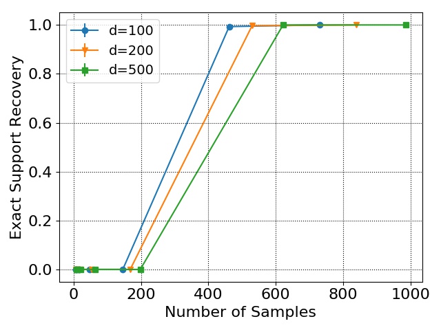
(a) Recovery of $S$ vs $n$

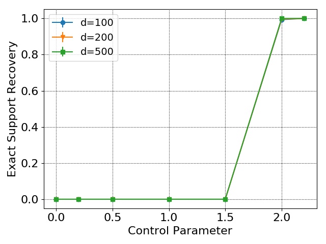
(b) Recovery of $S$ vs $\beta$

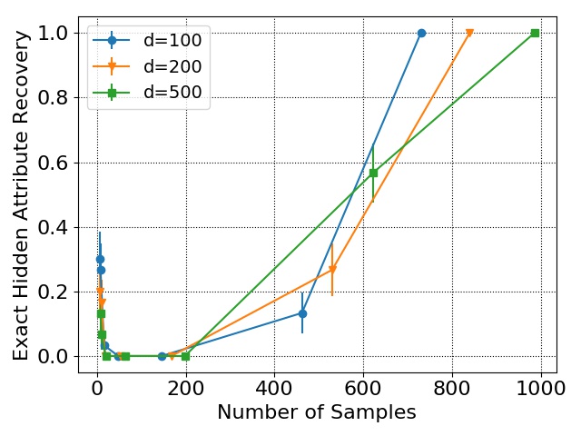
(c) Recovery of $\mathbf{Z}^{*}$ vs $n$

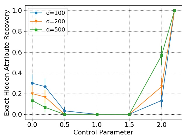
(d) Recovery of $\mathbf{Z}^{*}$ vs $\beta$

Figure 2: Left two: Exact support recovery of $w^{*}$ across $30$ runs. Right two: Exact hidden attribute recovery of $\mathbf{Z}^{*}$ across $30$ runs.

 

Supplementary Material: Fair Sparse Regression with Clustering: An Invex Relaxation for a Combinatorial Problem

 

Appendix A Proof of Lemma 1

Lemma 1

For $(w,\mathbf{Z})\in C$, the functions $f(w,\mathbf{Z})=\langle\mathbf{M}^{\prime}(w),\mathbf{Z}\rangle$ and $g(w,\mathbf{Z})=\langle a,w\rangle$ are $\eta$-invex for $\eta(w,\bar{w},\mathbf{Z},\bar{\mathbf{Z}})\triangleq\begin{bmatrix}w-\bar{w}\\ \mathbf{M}^{\prime}(\bar{w})^{-1}\mathbf{M}^{\prime}(w)(\mathbf{Z}-\bar{\mathbf{Z}})\end{bmatrix}$, where we abuse the vector/matrix notation for clarity of presentation, and avoid the vectorization of matrices.

Proof.

We need to prove the following two inequalities.

$$\begin{split}&f(w,\mathbf{Z})-f(\bar{w},\bar{\mathbf{Z}})-\langle\nabla_{\bar{w},\bar{\mathbf{Z}}}f(w,\mathbf{Z}),\eta(w,\bar{w},\mathbf{Z},\bar{\mathbf{Z}})\rangle\geq 0\,,\end{split}$$ (18)

$$\begin{split}&g(w,\mathbf{Z})-g(\bar{w},\bar{\mathbf{Z}})-\langle\nabla_{\bar{w},\bar{\mathbf{Z}}}g(w,\mathbf{Z}),\eta(w,\bar{w},\mathbf{Z},\bar{\mathbf{Z}})\rangle\geq 0\,.\end{split}$$ (19)

First, we observe that function $g(w,\mathbf{Z})$ only depends on $w$ and moreover, $\forall a\in^{d}$, $g(w,\mathbf{Z})$ is convex in $w$. Thus, the inequality (19) holds trivially. Note that $f(w,\mathbf{Z})=\langle\mathbf{M}^{\prime}(w),\mathbf{Z}\rangle=\sum_{ij}\mathbf{M}_{ij}^{\prime}(w)\mathbf{Z}_{ij}$. Then,

$$\begin{split}\frac{\partial{f(\bar{w},\bar{\mathbf{Z}})}}{\partial{w}}=\sum_{ij}\bar{\mathbf{Z}}_{ij}\frac{\partial{\mathbf{M}_{ij}^{\prime}(\bar{w})}}{\partial{w}},\;\;\;\frac{\partial{f(\bar{w},\bar{\mathbf{Z}})}}{\partial{\mathbf{Z}}}=\mathbf{M}^{\prime}(\bar{w})\end{split}$$

We further note that the diagonal elements of $\mathbf{M}^{\prime}(w)$ are convex with respect to $w$ and the off diagonal elements are linear. Therefore, we can write the following:

$$\begin{split}\mathbf{M}_{ii}^{\prime}(w)-\mathbf{M}_{ii}^{\prime}(\bar{w})&\geq\langle\frac{\partial{\mathbf{M}_{ii}^{\prime}(\bar{w})}}{\partial{w}},w-\bar{w}\rangle,\forall i\in[n+1]\\ \mathbf{M}_{ij}^{\prime}(w)-\mathbf{M}_{ij}^{\prime}(\bar{w})&=\langle\frac{\partial{\mathbf{M}_{ij}^{\prime}(\bar{w})}}{\partial{w}},w-\bar{w}\rangle,\forall i,j\in[n+1],i\neq j\end{split}$$

Since $\bar{\mathbf{Z}}_{ii}\geq 0$, it follows that

$$\begin{split}\bar{\mathbf{Z}}_{ij}\langle\frac{\partial{\mathbf{M}_{ij}^{\prime}(\bar{w})}}{\partial{w}},w-\bar{w}\rangle\leq\bar{\mathbf{Z}}_{ij}(\mathbf{M}_{ij}^{\prime}(w)-\mathbf{M}_{ij}^{\prime}(\bar{w}))\,.\end{split}$$

Now, we prove that $f(w,\mathbf{Z})$ is indeed $\eta$-invex, that is

$$\begin{split}&f(w,\mathbf{Z})-f(\bar{w},\bar{\mathbf{Z}})-\langle\nabla_{\bar{w},\bar{\mathbf{Z}}}f(w,\mathbf{Z}),\eta(w,\bar{w},\mathbf{Z},\bar{\mathbf{Z}})\rangle\\ &=\langle\mathbf{M}^{\prime}(w),\mathbf{Z}\rangle-\langle\mathbf{M}^{\prime}(\bar{w}),\bar{\mathbf{Z}}\rangle-\langle\sum_{ij}\bar{\mathbf{Z}}_{ij}\frac{\partial{\mathbf{M}_{ij}^{\prime}(\bar{w})}}{\partial{w}},w-\bar{w}\rangle-\langle\mathbf{M}^{\prime}(\bar{w}),\mathbf{M}^{\prime}(\bar{w})^{-1}\mathbf{M}^{\prime}(w)(\mathbf{Z}-\bar{\mathbf{Z}})\rangle\\ &\geq\langle\mathbf{M}^{\prime}(w),\mathbf{Z}\rangle-\langle\mathbf{M}^{\prime}(\bar{w}),\bar{\mathbf{Z}}\rangle-\sum_{ij}\bar{\mathbf{Z}}_{ij}(\mathbf{M}_{ij}^{\prime}(w)-\mathbf{M}_{ij}^{\prime}(\bar{w}))-\langle\mathbf{M}^{\prime}(w),\mathbf{Z}\rangle+\langle\mathbf{M}^{\prime}(w),\bar{\mathbf{Z}}\rangle\\ &=0\end{split}$$

This proves that $f(w,\mathbf{Z})$ is $\eta$-invex in $(w,\mathbf{Z})\in C$. ∎

Appendix B Mixed Integer Quadratic Program (MIQP) (4) is NP-Hard

In this section, we will show that the MIQP presented in (4) is at least as hard to solve as a $0-1$ Quadratic Program. It should be noted that MIQP (4) is stated for a fixed $\mathbf{X}$. However, since the entries in $\mathbf{X}$ are drawn from a sub-Gaussian distribution, matrix $\mathbf{X}$ can potentially realize any real matrix in ^n×d.

Lemma 9.

The Mixed Integer Quadratic Program (MIQP) (4) is NP-hard.

Proof.

We will consider the case when $\lambda_{n}=0$. Other cases will be at least as difficult as this case. First, we write optimization problem (4) in the following form:

$$\begin{split}&\min_{w\in^{d},\mathbf{z}\in\{-1,1\}^{n}}\frac{1}{2}w^{\intercal}(\frac{2}{n}\mathbf{X}^{\intercal}\mathbf{X})w+\mathbf{z}^{\intercal}\frac{2}{n}\gamma\mathbf{X}w+\frac{1}{2}\mathbf{z}^{\intercal}\frac{2}{n}\gamma^{2}\mathbf{I}\mathbf{z}-\frac{2}{n}\mathbf{y}^{\intercal}\mathbf{X}w-\frac{2}{n}\gamma\mathbf{y}^{\intercal}\mathbf{z}\\ &=\min_{\mathbf{z}\in\{-1,1\}^{n}}\left(\frac{1}{2}\mathbf{z}^{\intercal}\frac{2}{n}\gamma^{2}\mathbf{I}\mathbf{z}-\frac{2}{n}\gamma\mathbf{y}^{\intercal}\mathbf{z}+\left(\min_{w\in^{d}}\frac{1}{2}w^{\intercal}(\frac{2}{n}\mathbf{X}^{\intercal}\mathbf{X})w+(\mathbf{z}^{\intercal}\frac{2}{n}\gamma\mathbf{X}-\frac{2}{n}\mathbf{y}^{\intercal}\mathbf{X})w\right)\right)\end{split}$$ (20)

We observe that $w=(\mathbf{X}^{\intercal}\mathbf{X})^{\dagger}\mathbf{X}^{\intercal}(-\gamma\mathbf{z}+\mathbf{y})$ solves the nested optimization problem, where $(\cdot)^{\dagger}$ denotes the pseudo-inverse. Thus, substituting the optimal value of $w$, we get the following optimization problem:

$$\begin{split}\min_{\mathbf{z}\in\{-1,1\}^{n}}\frac{\gamma^{2}}{n}\mathbf{z}^{\intercal}(\mathbf{I}-\mathbf{X}(\mathbf{X}^{\intercal}\mathbf{X})^{\dagger}\mathbf{X}^{\intercal})\mathbf{z}-\frac{2\gamma}{n}\mathbf{y}^{\intercal}(\mathbf{I}-\mathbf{X}(\mathbf{X}^{\intercal}\mathbf{X})^{\dagger}\mathbf{X}^{\intercal})\mathbf{z}\end{split}$$ (21)

Observe that $I-\mathbf{X}(\mathbf{X}^{\intercal}\mathbf{X})^{\dagger}\mathbf{X}^{\intercal}$ can potentially be any fixed real matrix in ^n×n. By simply substituting $\mathbf{z}^{\prime}=\frac{\mathbf{z}+1}{2}$, we get a $0-1$ Quadratic Program which is known to be NP-Hard [Billionnet(2010)]. ∎

Appendix C Proof of Lemma 2

Lemma 2

If Assumption 1 holds and $n=\Omega(\frac{s+\log d}{C_{\min}^{2}})$, then ${\rm{eig}}_{\min}(\hat{\mathbf{H}}_{SS})\geq\frac{C_{\min}}{2}$ with probability at least $1-\mathcal{O}(\frac{1}{d})$.

Proof.

By the Courant-Fischer variational representation [Horn & Johnson(2012)]:

$$\begin{split}{\rm{eig}}_{\min}(\mathbb{E}(XX^{\intercal})_{SS})=\min_{\|y\|_{2}=1}y^{\intercal}\mathbb{E}(XX^{\intercal})_{SS}y&=\min_{\|y\|_{2}=1}y^{\intercal}(\mathbb{E}(XX^{\intercal})_{SS}-\frac{1}{n}\mathbf{X}^{\intercal}_{S}\mathbf{X}_{S}+\frac{1}{n}\mathbf{X}^{\intercal}_{S}\mathbf{X}_{S})y\\ &\leq y^{\intercal}(\mathbb{E}(XX^{\intercal})_{SS}-\frac{1}{n}\mathbf{X}^{\intercal}_{S}\mathbf{X}_{S}+\frac{1}{n}\mathbf{X}^{\intercal}_{S}\mathbf{X}_{S})y\\ &=y^{\intercal}(\mathbb{E}(XX^{\intercal})_{SS}-\frac{1}{n}\mathbf{X}^{\intercal}_{S}\mathbf{X}_{S})y+y^{\intercal}\frac{1}{n}\mathbf{X}^{\intercal}_{S}\mathbf{X}_{S}y\end{split}$$ (22)

It follows that

$$\begin{split}{\rm{eig}}_{\min}(\frac{1}{n}\mathbf{X}^{\intercal}_{S}\mathbf{X}_{S})\geq C_{\min}-\|\mathbb{E}(XX^{\intercal})_{SS}-\frac{1}{n}\mathbf{X}^{\intercal}_{S}\mathbf{X}_{S}\|_{2}\end{split}$$ (23)

The term $\|\mathbb{E}(XX^{\intercal})_{SS}-\frac{1}{n}\mathbf{X}^{\intercal}_{S}\mathbf{X}_{S}\|_{2}$ can be bounded using Proposition 2.1 in [Vershynin(2012)] for sub-Gaussian random variables. In particular,

$$\begin{split}\mathbb{P}(\|\mathbb{E}(XX^{\intercal})_{SS}-\frac{1}{n}\mathbf{X}^{\intercal}_{S}\mathbf{X}_{S}\|_{2}\geq\epsilon)\leq 2\exp(-c\epsilon^{2}n+s)\end{split}$$ (24)

for some constant $c>0$. Taking $\epsilon=\frac{C_{\min}}{2}$, we show that ${\rm{eig}}_{\min}(\frac{1}{n}\mathbf{X}^{\intercal}_{S}\mathbf{X}_{S})\geq\frac{C_{\min}}{2}$ with probability at least $1-2\exp(-\frac{cC_{\min}^{2}n}{4}+s)$. ∎

Appendix D Proof of Lemma 3

Lemma 3

If Assumption 2 holds and $n=\Omega(\frac{s^{3}(\log s+\log d)}{\tau(C_{\min},\alpha,\sigma,\Sigma)})$, then $\|\hat{\mathbf{H}}_{S^{c}S}\hat{\mathbf{H}}_{SS}^{-1}\|_{\infty}\leq 1-\frac{\alpha}{2}$ with probability at least $1-\mathcal{O}(\frac{1}{d})$ where $\tau(C_{\min},\alpha,\sigma,\Sigma)$ is a constant independent of $n,d$ and $s$.

Proof.

Before we prove the result of Lemma 3, we will prove a helper lemma.

Lemma 10.

If Assumption 2 holds then for some $\delta>0$, the following inequalities hold:

$$\begin{split}&\mathbb{P}(\|\hat{\mathbf{H}}_{S^{c}S}-\mathbf{H}_{S^{c}S}\|_{\infty}\geq\delta)\leq 4(d-s)s\exp(-\frac{n\delta^{2}}{128s^{2}(1+4\sigma^{2})\max_{l}\Sigma_{ll}^{2}})\\ &\mathbb{P}(\|\hat{\mathbf{H}}_{SS}-\mathbf{H}_{SS}\|_{\infty}\geq\delta)\leq 4s^{2}\exp(-\frac{n\delta^{2}}{128s^{2}(1+4\sigma^{2})\max_{l}\Sigma_{ll}^{2}})\\ &\mathbb{P}(\|(\hat{\mathbf{H}}_{SS})^{-1}-(\mathbf{H}_{SS})^{-1}\|_{\infty}\geq\delta)\leq 2\exp(-\frac{c\delta^{2}C_{\min}^{4}n}{4s}+s)+2\exp(-\frac{cC_{\min}^{2}n}{4}+s)\end{split}$$ (25)

Proof.

Let $A_{ij}$ be $(i,j)$-th entry of $\hat{\mathbf{H}}_{S^{c}S}-\mathbf{H}_{S^{c}S}$. Clearly, $\mathbb{E}(A_{ij})=0$. By using the definition of the $\|\cdot\|_{\infty}$ norm, we can write:

$$\begin{split}\mathbb{P}(\|\hat{\mathbf{H}}_{S^{c}S}-\mathbf{H}_{S^{c}S}\|_{\infty}\geq\delta)&=\mathbb{P}(\max_{i\in S^{c}}\sum_{j\in S}|A_{ij}|\geq\delta)\\ &\leq(d-s)\mathbb{P}(\sum_{j\in S}|A_{ij}|\geq\delta)\\ &\leq(d-s)s\mathbb{P}(|A_{ij}|\geq\frac{\delta}{s})\end{split}$$ (26)

where the second last inequality comes as a result of the union bound across entries in $S^{c}$ and the last inequality is due to the union bound across entries in $S$. Recall that $X_{i},i\in[d]$ are zero mean random variables with covariance $\Sigma$ and each $\frac{X_{i}}{\sqrt{\Sigma_{ii}}}$ is a sub-Gaussian random variable with parameter $\sigma$. Using the results from Lemma 1 of [Ravikumar et al.(2011)], for some $\delta\in(0,s\max_{l}\Sigma_{ll}8(1+4\sigma^{2}))$, we can write:

$$\begin{split}\mathbb{P}(|A_{ij}|\geq\frac{\delta}{s})\leq 4\exp(-\frac{n\delta^{2}}{128s^{2}(1+4\sigma^{2})\max_{l}\Sigma_{ll}^{2}})\end{split}$$ (27)

Therefore,

$$\begin{split}&\mathbb{P}(\|\hat{\mathbf{H}}_{S^{c}S}-\mathbf{H}_{S^{c}S}\|_{\infty}\geq\delta)\leq 4(d-s)s\exp(-\frac{n\delta^{2}}{128s^{2}(1+4\sigma^{2})\max_{l}\Sigma_{ll}^{2}})\end{split}$$ (28)

Similarly, we can show that

$$\begin{split}&\mathbb{P}(\|\hat{\mathbf{H}}_{SS}-\mathbf{H}_{SS}\|_{\infty}\geq\delta)\leq 4s^{2}\exp(-\frac{n\delta^{2}}{128s^{2}(1+4\sigma^{2})\max_{l}\Sigma_{ll}^{2}})\end{split}$$ (29)

Next, we will show that the third inequality in (25) holds. Note that

$$\begin{split}\|(\hat{\mathbf{H}}_{S^{c}S})^{-1}-(\mathbf{H}_{S^{c}S})^{-1}\|_{\infty}&=\|(\mathbf{H}_{SS})^{-1}(\mathbf{H}_{SS}-\hat{\mathbf{H}}_{SS})(\hat{\mathbf{H}}_{SS})^{-1}\|_{\infty}\\ &\leq\sqrt{s}\|(\mathbf{H}_{SS})^{-1}(\mathbf{H}_{SS}-\hat{\mathbf{H}}_{SS})(\hat{\mathbf{H}}_{SS})^{-1}\|_{2}\\ &\leq\sqrt{s}\|(\mathbf{H}_{SS})^{-1}\|_{2}\|(\mathbf{H}_{SS}-\hat{\mathbf{H}}_{SS})\|_{2}\|(\hat{\mathbf{H}}_{SS})^{-1}\|_{2}\\ \end{split}$$ (30)

Note that $\|\mathbf{H}_{SS}\|_{2}\geq C_{\min}$, thus $\|(\mathbf{H}_{SS})^{-1}\|_{2}\leq\frac{1}{C_{\min}}$. Similarly, $\|\mathbf{H}_{SS}\|_{2}\geq\frac{C_{\min}}{2}$ with probability at least $1-2\exp(-\frac{cC_{\min}^{2}n}{4}+s)$. We also have $\|(\mathbf{H}_{SS}-\hat{\mathbf{H}}_{SS})\|_{2}\leq\epsilon$ with probability at least $1-2\exp(-c\epsilon^{2}n+s)$. Taking $\epsilon=\delta\frac{C_{\min}^{2}}{2\sqrt{s}}$, we get

$$\begin{split}\mathbb{P}(\|(\mathbf{H}_{SS}-\hat{\mathbf{H}}_{SS})\|_{2}\geq\delta\frac{C_{\min}^{2}}{2\sqrt{s}})\leq 2\exp(-\frac{c\delta^{2}C_{\min}^{4}n}{4s}+s)\end{split}$$ (31)

It follows that $\|(\hat{\mathbf{H}}_{SS})^{-1}-(\mathbf{H}_{SS})^{-1}\|_{\infty}\leq\delta$ with probability at least $1-2\exp(-\frac{c\delta^{2}C_{\min}^{4}n}{4s}+s)-2\exp(-\frac{cC_{\min}^{2}n}{4}+s)$. ∎

Now we are ready to show that the statement of Lemma 3 holds using the results from Lemma 10. We will rewrite $\hat{\mathbf{H}}_{S^{c}S}(\hat{\mathbf{H}}_{SS})^{-1}$ as the sum of four different terms:

$$\begin{split}\hat{\mathbf{H}}_{S^{c}S}(\hat{\mathbf{H}}_{SS})^{-1}=T_{1}+T_{2}+T_{3}+T_{4},\end{split}$$ (32)

where

$$\begin{split}T_{1}&\triangleq\hat{\mathbf{H}}_{S^{c}S}((\hat{\mathbf{H}}_{SS})^{-1}-(\mathbf{H}_{SS})^{-1})\\ T_{2}&\triangleq(\hat{\mathbf{H}}_{S^{c}S}-\mathbf{H}_{S^{c}S})(\mathbf{H}_{SS})^{-1}\\ T_{3}&\triangleq(\hat{\mathbf{H}}_{S^{c}S}-\mathbf{H}_{S^{c}S})((\hat{\mathbf{H}}_{SS})^{-1}-(\mathbf{H}_{SS})^{-1})\\ T_{4}&\triangleq\mathbf{H}_{S^{c}S}(\mathbf{H}_{SS})^{-1}\,.\end{split}$$ (33)

Then it follows that $\|\hat{\mathbf{H}}_{S^{c}S}(\hat{\mathbf{H}}_{SS})^{-1}\|_{\infty}\leq\|T_{1}\|_{\infty}+\|T_{2}\|_{\infty}+\|T_{3}\|_{\infty}+\|T_{4}\|_{\infty}$. Now, we will bound each term separately. First, recall that Assumption 2 ensures that $\|T_{4}\|_{\infty}\leq 1-\alpha$.

Controlling $T_{1}$.

We can rewrite $T_{1}$ as,

$$\begin{split}T_{1}=-\mathbf{H}_{S^{c}S}(\mathbf{H}_{SS})^{-1}(\hat{\mathbf{H}}_{SS}-\mathbf{H}_{SS})(\hat{\mathbf{H}}_{SS})^{-1}\end{split}$$ (34)

then,

$$\begin{split}\|T_{1}\|_{\infty}&=\|\mathbf{H}_{S^{c}S}(\mathbf{H}_{SS})^{-1}(\hat{\mathbf{H}}_{SS}-\mathbf{H}_{SS})(\hat{\mathbf{H}}_{SS})^{-1}\|_{\infty}\\ &\leq\|\mathbf{H}_{S^{c}S}(\mathbf{H}_{SS})^{-1}\|_{\infty}\|(\hat{\mathbf{H}}_{SS}-\mathbf{H}_{SS})\|_{\infty}\|(\hat{\mathbf{H}}_{SS})^{-1}\|_{\infty}\\ &\leq(1-\alpha)\|(\hat{\mathbf{H}}_{SS}-\mathbf{H}_{SS})\|_{\infty}\sqrt{s}\|(\hat{\mathbf{H}}_{SS})^{-1}\|_{2}\\ &\leq(1-\alpha)\|(\hat{\mathbf{H}}_{SS}-\mathbf{H}_{SS})\|_{\infty}\frac{2\sqrt{s}}{C_{\min}}\\ &\leq\frac{\alpha}{6}\end{split}$$ (35)

The last inequality holds with probability at least $1-2\exp(-\frac{cC_{\min}^{2}n}{4}+s)-4s^{2}\exp(-\frac{nC_{\min}^{2}\alpha^{2}}{18432(1-\alpha)^{2}s^{3}(1+4\sigma^{2})\max_{l}\Sigma_{ll}^{2}})$ by taking $\delta=\frac{C_{\min}\alpha}{12(1-\alpha)\sqrt{s}}$.

Controlling $T_{2}$.

Recall that $T_{2}=(\hat{\mathbf{H}}_{S^{c}S}-\mathbf{H}_{S^{c}S})(\mathbf{H}_{SS})^{-1}$. Thus,

$$\begin{split}\|T_{2}\|_{\infty}&\leq\sqrt{s}\|(\mathbf{H}_{SS})^{-1}\|_{2}\|(\hat{\mathbf{H}}_{S^{c}S}-\mathbf{H}_{S^{c}S})\|_{\infty}\\ &\leq\frac{\sqrt{s}}{C_{\min}}\|(\hat{\mathbf{H}}_{S^{c}S}-\mathbf{H}_{S^{c}S})\|_{\infty}\\ &\leq\frac{\alpha}{6}\end{split}$$ (36)

The last inequality holds with probability at least $1-4(d-s)s\exp(-\frac{nC_{\min}^{2}\alpha^{2}}{4608s^{3}(1+4\sigma^{2})\max_{l}\Sigma_{ll}^{2}})$ by choosing $\delta=\frac{C_{\min}\alpha}{6\sqrt{s}}$.

Controlling $T_{3}$.

Note that,

$$\begin{split}\|T_{3}\|_{\infty}&\leq\|(\hat{\mathbf{H}}_{S^{c}S}-\mathbf{H}_{S^{c}S})\|_{\infty}\|((\hat{\mathbf{H}}_{SS})^{-1}-(\mathbf{H}_{SS})^{-1})\|_{\infty}\\ &\leq\frac{\alpha}{6}\end{split}$$ (37)

The last inequality holds with probability at least $1-4(d-s)s\exp(-\frac{n\alpha}{768s^{2}(1+4\sigma^{2})\max_{l}\Sigma_{l}l^{2}})-2\exp(-\frac{c\alpha C_{\min}^{4}n}{24s}+s)-2\exp(-\frac{cC_{\min}^{2}n}{4}+s)$ by choosing $\delta=\sqrt{\frac{\alpha}{6}}$ in the first and third inequality of equation (25). By combining all the above results, we prove Lemma 3. ∎

Appendix E Proof of Lemma 4

Lemma 4

If Assumptions 1 and 2 hold, $\lambda_{n}\geq\frac{128\rho k}{\alpha}\frac{\sqrt{\log d}}{n}$ and $n=\Omega(\frac{s^{3}\log d}{\tau_{1}(C_{\min},\alpha,\sigma,\Sigma,\rho)})$, then the setting of $w$ and $\mathbf{Z}$ from equation (13) satisfies the stationarity condition (8) with probability at least $1-\mathcal{O}(\frac{1}{d})$, where $\tau_{1}(C_{\min},\alpha,\sigma,\Sigma,\rho)$ is a constant independent of $d,s$ or $n$.

Proof.

Consider the following optimization problem:

$$\begin{split}\begin{matrix}\min_{w}&\frac{1}{n}(\mathbf{X}w+\gamma\mathbf{z}^{*}-\mathbf{y})^{\intercal}(\mathbf{X}w+\gamma\mathbf{z}^{*}-\mathbf{y})+\lambda_{n}\|w\|_{1}\end{matrix}\end{split}$$ (38)

Observe that the above problem is a transformation of optimization problem (6) by fixing $\mathbf{Z}=\mathbf{Z}^{*}$. With infinite samples (i.e., $n\to\infty,\lambda_{n}\to 0$), optimization problem (38) is equivalent to the following population version:

$$\begin{split}\begin{matrix}\min_{w}&\mathbb{E}((Xw+\gamma z^{*}-y)^{\intercal}(Xw+\gamma z^{*}-y))\end{matrix}\,.\end{split}$$ (39)

Clearly, due to Assumption 1, $w^{*}$ is the unique optimal solution to (39). Let $\tilde{w}$ be the solution to the optimization problem (38). Notice that after replacing $\mathbf{Z}$ with $\mathbf{Z}^{*}$ the stationarity condition (8) is same as the stationarity condition for optimization problem (38):

$$\begin{split}&\frac{\partial{L(w,\mathbf{Z};\mathbf{\mu},\Lambda)}}{\partial{w}}=\mathbf{0}_{d\times 1}\end{split}$$ (40)

The above simplifies into the following:

$$\begin{split}\frac{2}{n}\mathbf{X}^{\intercal}\mathbf{X}\tilde{w}-\frac{2}{n}\mathbf{X}^{\intercal}\mathbf{y}+\frac{2\gamma}{n}\mathbf{X}^{\intercal}\mathbf{z}^{*}+\lambda_{n}\mathbf{g}=\mathbf{0}_{d\times 1}\end{split}$$

Substituting $\mathbf{y}$ from equation (2), we get:

$$\begin{split}\frac{2}{n}\mathbf{X}^{\intercal}\mathbf{X}\Delta-\frac{2}{n}\mathbf{X}^{\intercal}\mathbf{e}+\lambda_{n}\mathbf{g}=\mathbf{0}_{d\times 1}\,,\end{split}$$ (41)

where $\Delta$ is a short form notation for $\tilde{w}-w^{*}$. To prove our claim, it suffices to show that $\tilde{w}=(\tilde{w}_{S},\mathbf{0}_{d-s\times 1})$ satisfies the stationarity condition (41). This will be true iff $\mathbf{g}_{S}\in\{-1,1\}^{s}$ and $\mathbf{g}_{S^{c}}\in[-1,1]^{d-s}$. In particular, if we start with $w=[w_{S},\mathbf{0}_{d-s\times 1}]$ and show that $\|\mathbf{g}_{S^{c}}\|_{\infty}<1$, then our claim holds. To show this, we replace $w$ with $[w_{S},\mathbf{0}_{d-s\times 1}]$ and rewrite equation (41) in two parts:

$$\begin{split}\frac{1}{n}\mathbf{X}_{S}^{\intercal}\mathbf{X}_{S}\Delta_{S}-\frac{1}{n}\mathbf{X}_{S}^{\intercal}\mathbf{e}+\frac{\lambda_{n}}{2}\mathbf{g}_{S}=\mathbf{0}_{s\times 1}\,,\end{split}$$ (42)

and

$$\begin{split}\frac{1}{n}\mathbf{X}_{S^{c}}^{\intercal}\mathbf{X}_{S}\Delta_{S}-\frac{1}{n}\mathbf{X}_{S^{c}}^{\intercal}\mathbf{e}+\frac{\lambda_{n}}{2}\mathbf{g}_{S^{c}}=\mathbf{0}_{d-s\times 1}\,,\end{split}$$ (43)

where $\Delta_{S}=w_{S}-w_{S}^{*}$. From equation (42):

$$\begin{split}\Delta_{S}=(\frac{1}{n}\mathbf{X}_{S}^{\intercal}\mathbf{X}_{S})^{-1}\frac{1}{n}\mathbf{X}_{S}^{\intercal}\mathbf{e}-(\frac{1}{n}\mathbf{X}_{S}^{\intercal}\mathbf{X}_{S})^{-1}\frac{\lambda_{n}}{2}\mathbf{g}_{S}\end{split}$$

By substituting $\Delta_{S}$ in equation (43), we get:

$$\begin{split}&\hat{\mathbf{H}}_{S^{c}S}(\hat{\mathbf{H}}_{SS}^{-1}\frac{1}{n}\mathbf{X}_{S}^{\intercal}\mathbf{e}-\hat{\mathbf{H}}_{SS}^{-1}\frac{\lambda_{n}}{2}\mathbf{g}_{S})-\frac{1}{n}\mathbf{X}_{S^{c}}^{\intercal}\mathbf{e}+\frac{\lambda_{n}}{2}\mathbf{g}_{S^{c}}=\mathbf{0}_{d-s\times 1}\end{split}$$

By rearranging terms and using the triangle inequality, we get the following:

$$\begin{split}&\|\frac{\lambda_{n}}{2}\mathbf{g}_{S^{c}}\|_{\infty}\leq\|\hat{\mathbf{H}}_{S^{c}S}\hat{\mathbf{H}}_{SS}^{-1}\frac{1}{n}\mathbf{X}_{S}^{\intercal}\mathbf{e}\|_{\infty}+\|\hat{\mathbf{H}}_{S^{c}S}\hat{\mathbf{H}}_{SS}^{-1}\frac{\lambda_{n}}{2}\mathbf{g}_{S}\|_{\infty}+\|\frac{1}{n}\mathbf{X}_{S^{c}}^{\intercal}\mathbf{e}\|_{\infty}\end{split}$$

Using the norm inequality $\|Ab\|_{\infty}\leq\|A\|_{\infty}\|b\|_{\infty}$ and noticing that $\|\mathbf{g}_{S}\|_{\infty}\leq 1$, it follows that:

$$\begin{split}&\|\frac{\lambda_{n}}{2}\mathbf{g}_{S^{c}}\|_{\infty}\leq\|\hat{\mathbf{H}}_{S^{c}S}\hat{\mathbf{H}}_{SS}^{-1}\|_{\infty}(\|\frac{1}{n}\mathbf{X}_{S}^{\intercal}\mathbf{e}\|_{\infty}+\frac{\lambda_{n}}{2})+\|\frac{1}{n}\mathbf{X}_{S^{c}}^{\intercal}\mathbf{e}\|_{\infty}\end{split}$$

Furthermore, using Lemma 3, $\|\hat{\mathbf{H}}_{S^{c}S}\hat{\mathbf{H}}_{SS}^{-1}\|_{\infty}\leq 1-\frac{\alpha}{2}$ with probability at least $1-\exp(-\frac{n\tau(C_{\min},\alpha,\sigma,\Sigma)}{s^{2}}+\log s)$:

$$\begin{split}&\|\mathbf{g}_{S^{c}}\|_{\infty}\leq(1-\frac{\alpha}{2})(\|\frac{2}{\lambda_{n}}\frac{1}{n}\mathbf{X}_{S}^{\intercal}\mathbf{e}\|_{\infty}+1)+\|\frac{2}{\lambda_{n}}\frac{1}{n}\mathbf{X}_{S^{c}}^{\intercal}\mathbf{e}\|_{\infty}\end{split}$$

Next, we will need to bound $\|\frac{1}{n}\mathbf{X}_{S}^{\intercal}\mathbf{e}\|_{\infty}$ and $\|\frac{1}{n}\mathbf{X}_{S^{c}}^{\intercal}\mathbf{e}\|_{\infty}$ which we do in the following lemma:

Lemma 11.

Let $\lambda_{n}\geq\frac{128\rho k}{\alpha}\frac{\sqrt{\log d}}{n}$ and $n\geq\frac{\log d}{(1-\frac{\alpha}{2})^{2}}$. Then the following holds true:

$$\begin{split}&\mathbb{P}(\|\frac{2}{\lambda_{n}}\frac{1}{n}\mathbf{X}_{S}^{\intercal}\mathbf{e}\|_{\infty}\geq\frac{\alpha}{8-4\alpha})\leq\mathcal{O}(\frac{1}{d}),\quad\mathbb{P}(\|\frac{2}{\lambda_{n}}\frac{1}{n}\mathbf{X}_{S^{c}}^{\intercal}\mathbf{e}\|_{\infty}\geq\frac{\alpha}{8})\leq\mathcal{O}(\frac{1}{d})\end{split}$$

Using results from Lemma 11, we show that $\|\mathbf{g}_{S^{c}}\|_{\infty}\leq 1-\frac{\alpha}{4}$ with probability at least $1-\mathcal{O}(\frac{1}{d})$. This ensures that $\tilde{w}=(\tilde{w}_{S},\mathbf{0}_{d-s\times 1})$ indeed satisfies the stationarity condition (8). ∎

Appendix F Proof of Lemma 11

Lemma 11

Let $\lambda_{n}\geq\frac{128\rho k}{\alpha}\frac{\sqrt{\log d}}{n}$ and $n\geq\frac{\log d}{(1-\frac{\alpha}{2})^{2}}$. Then the following holds true:

$$\begin{split}\mathbb{P}(\|\frac{2}{\lambda_{n}}\frac{1}{n}\mathbf{X}_{S}^{\intercal}\mathbf{e}\|_{\infty}&\geq\frac{\alpha}{8-4\alpha})\leq\mathcal{O}(\frac{1}{d})\\ \mathbb{P}(\|\frac{2}{\lambda_{n}}\frac{1}{n}\mathbf{X}_{S^{c}}^{\intercal}\mathbf{e}\|_{\infty}&\geq\frac{\alpha}{8})\leq\mathcal{O}(\frac{1}{d})\end{split}$$ (44)

Proof.

We will start with $\frac{1}{n}\mathbf{X}_{S}^{\intercal}\mathbf{e}$. We take the $i$-th entry of $\frac{1}{n}\mathbf{X}_{S}^{\intercal}\mathbf{e}$ for some $i\in S$. Note that

$$\begin{split}|\frac{1}{n}\mathbf{X}_{i.}^{\intercal}\mathbf{e}|=|\frac{1}{n}\sum_{j=1}^{n}\mathbf{X}_{ji}\mathbf{e}_{j}|\end{split}$$ (45)

Recall that $\mathbf{X}_{ji}$ is a sub-Gaussian random variable with parameter $\rho^{2}$ and $\mathbf{e}_{j}$ is a sub-Gaussian random variable with parameter $\sigma_{e}^{2}$. Then, $\frac{\mathbf{X}_{ji}}{\rho}\frac{\mathbf{e}_{j}}{\sigma_{e}}$ is a sub-exponential random variable with parameters $(4\sqrt{2},2)$. Using the concentration bounds for the sum of independent sub-exponential random variables [Wainwright(2019)], we can write:

$$\begin{split}\mathbb{P}(|\frac{1}{n}\sum_{j=1}^{n}\frac{\mathbf{X}_{ji}}{\rho}\frac{\mathbf{e}_{j}}{\sigma_{e}}|\geq t)\leq 2\exp(-\frac{nt^{2}}{64}),\;0\leq t\leq 8\end{split}$$ (46)

Taking a union bound across $i\in S$:

$$\begin{split}&\mathbb{P}(\exists i\in S\mid|\frac{1}{n}\sum_{j=1}^{n}\frac{\mathbf{X}_{ji}}{\rho}\frac{\mathbf{e}_{j}}{\sigma_{e}}|\geq t)\leq 2s\exp(-\frac{nt^{2}}{64})\\ &0\leq t\leq 8\end{split}$$ (47)

Taking $t=\frac{\lambda_{n}t}{2\rho\sigma_{e}}$, we get:

$$\begin{split}&\mathbb{P}(\exists i\in S\mid|\frac{2}{\lambda_{n}}\frac{1}{n}\sum_{j=1}^{n}\mathbf{X}_{ji}\mathbf{e}_{j}|\geq t)\leq 2s\exp(-\frac{n\lambda_{n}^{2}t^{2}}{256\rho^{2}\sigma_{e}^{2}})\\ &0\leq t\leq 16\frac{\rho\sigma_{e}}{\lambda_{n}}\end{split}$$ (48)

It follows that $\|\frac{2}{\lambda}\frac{1}{n}\mathbf{X}_{S}^{\intercal}\mathbf{e}\|_{\infty}\leq t$ with probability at least $1-2s\exp(-\frac{n\lambda_{n}^{2}t^{2}}{256\rho^{2}\sigma_{e}^{2}})$.

Using a similar argument, we can show that $\|\frac{2}{\lambda}\frac{1}{n}\mathbf{X}_{S^{c}}^{\intercal}\mathbf{e}\|_{\infty}\leq t$ with probability at least $1-2(d-s)\exp(-\frac{n\lambda_{n}^{2}t^{2}}{256\rho^{2}\sigma_{e}^{2}})$. Taking $t=\frac{\alpha}{8-4\alpha}$ and $\frac{\alpha}{8}$ in the first and second inequality of Lemma 11 and choosing the provided setting of $\lambda_{n}$ and $n$ completes our proof. ∎

Appendix G Proof of Lemma 8

Lemma 8

If Assumptions 1 and 2 hold, $\lambda_{n}\geq\frac{128\rho k\sqrt{\log d}}{\alpha n}$ and $n=\Omega(\frac{s^{3}\log d}{\tau_{2}(C_{\min},\rho,k)})$, then $\|\Delta_{S}\|_{2}\leq\frac{2\lambda_{n}\sqrt{s}}{C_{\min}}$ with probability at least $1-\mathcal{O}(\frac{1}{d})$ where $\tau_{2}(C_{\min},\rho,k)$ is a constant independent of $s,d$ or $n$.

Proof.

Using results from Lemma 4, we can write:

$$\begin{split}\|\Delta_{S}\|_{2}\leq\|\hat{\mathbf{H}}_{SS}^{-1}\frac{1}{n}\mathbf{X}_{S}^{\intercal}\mathbf{e}\|_{2}+\|\hat{\mathbf{H}}_{SS}^{-1}\frac{\lambda_{n}}{2}\mathbf{g}_{S}\|_{2}\end{split}$$

Using the norm inequality $\|Ab\|_{2}\leq\|A\|_{2}\|b\|_{2}$ and noticing that $\|\mathbf{g}_{S}\|_{2}\leq\sqrt{s}$, we can rewrite the above equation as:

$$\begin{split}\|\Delta_{S}\|_{2}\leq\|\hat{\mathbf{H}}_{SS}^{-1}\|_{2}(\|\frac{1}{n}\mathbf{X}_{S}^{\intercal}\mathbf{e}\|_{2}+\frac{\lambda_{n}}{2}\sqrt{s})\end{split}$$

Using Assumption 1 and results from Lemma 2 and substituting $\|\hat{\mathbf{H}}_{SS}^{-1}\|_{2}\leq\frac{2}{C_{\min}}$ in the above inequality, we get:

$$\begin{split}\|\Delta_{S}\|_{2}\leq\frac{2}{C_{\min}}(\|\frac{1}{n}\mathbf{X}_{S}^{\intercal}\mathbf{e}\|_{2}+\frac{\lambda_{n}}{2}\sqrt{s})\end{split}$$

We present the next lemma to bound the term $\|\frac{1}{n}\mathbf{X}_{S}^{\intercal}\mathbf{e}\|_{2}$.

Lemma 12.

If $\lambda_{n}\geq\frac{128\rho k}{\alpha}\frac{\sqrt{\log d}}{n}$ and $n=\Omega(\frac{s^{3}\log d}{\tau_{2}(C_{\min},\rho,k)})$, then $\|\frac{1}{n}\mathbf{X}_{S}^{\intercal}\mathbf{e}\|_{2}\leq\sqrt{s}\frac{\lambda_{n}}{2}$ with probability at least $1-\mathcal{O}(\frac{1}{d})$.

We take $t=\frac{\lambda_{n}}{2}$ in the above lemma and get $\|\Delta\|_{2}\leq\frac{2\lambda_{n}\sqrt{s}}{C_{\min}}$ with probability at least $1-\mathcal{O}(\frac{1}{d})$. ∎

Appendix H Proof of Lemma 12

Lemma 12

If $\lambda_{n}\geq\frac{128\rho k}{\alpha}\frac{\sqrt{\log d}}{n}$ and $n=\Omega(\frac{s^{3}\log d}{\tau_{2}(C_{\min},\rho,k)})$, then $\|\frac{1}{n}\mathbf{X}_{S}^{\intercal}\mathbf{e}\|_{2}\leq\sqrt{s}\frac{\lambda_{n}}{2}$ with probability at least $1-\mathcal{O}(\frac{1}{d})$.

Proof.

We take the $i$-th entry of $\frac{1}{n}\mathbf{X}_{S}^{\intercal}\mathbf{e}$ for some $i\in S$. Note that

$$\begin{split}|\frac{1}{n}\mathbf{X}_{i.}^{\intercal}\mathbf{e}|=|\frac{1}{n}\sum_{j=1}^{n}\mathbf{X}_{ji}\mathbf{e}_{j}|\end{split}$$ (49)

Recall that $\mathbf{X}_{ji}$ is a sub-Gaussian random variable with parameter $\rho$ and $\mathbf{e}_{j}$ is a sub-Gaussian random variable with parameter $\sigma_{e}^{2})$. Then, $\frac{\mathbf{X}_{ji}}{\rho}\frac{\mathbf{e}_{j}}{\sigma_{e}}$ is a sub-exponential random variable with parameters $(4\sqrt{2},2)$. Using the concentration bounds for the sum of independent sub-exponential random variables [Wainwright(2019)], we can write:

$$\begin{split}\mathbb{P}(|\frac{1}{n}\sum_{j=1}^{n}\frac{\mathbf{X}_{ji}}{\rho}\frac{\mathbf{e}_{j}}{\sigma_{e}}|\geq t)\leq 2\exp(-\frac{nt^{2}}{64}),\;0\leq t\leq 8\end{split}$$ (50)

Taking a union bound across $i\in S$, we get

$$\begin{split}&\mathbb{P}(\exists i\in S\mid|\frac{1}{n}\sum_{j=1}^{n}\frac{\mathbf{X}_{ji}}{\rho}\frac{\mathbf{e}_{j}}{\sigma_{e}}|\geq t)\leq 2s\exp(-\frac{nt^{2}}{64}),\\ &0\leq t\leq 8\end{split}$$ (51)

It follows that $\|\frac{1}{n}\mathbf{X}_{S}^{\intercal}\mathbf{e}\|_{2}\leq\sqrt{s}t$ with probability at least $1-2s\exp(-\frac{nt^{2}}{64\rho^{2}\sigma_{e}^{2}})$ for some $0\leq t\leq 8\rho\sigma_{e}$. ∎

Appendix I Proof of Corollary 1

Corollary 1

If Assumptions 1 and 2 hold, $\lambda_{n}\geq\frac{128\rho k}{\alpha}\frac{\sqrt{\log d}}{n}$ and $n=\Omega(\frac{s^{3}\log d}{\tau_{1}(C_{\min},\alpha,\sigma,\Sigma,\rho)})$, then the following statements are true with probability at least $1-\mathcal{O}(\frac{1}{n})$:

1. The solution $\mathbf{Z}$ correctly recovers hidden attribute for each sample, i.e., $\mathbf{Z}=\mathbf{Z}^{*}=\zeta^{*}{\zeta^{*}}^{\intercal}$.

2. The support of recovered regression parameter $\tilde{w}$ matches exactly with the support of $w^{*}$.

3. If $\min_{i\in S}|w_{i}^{*}|\geq\frac{4\lambda_{n}\sqrt{s}}{C_{\min}}$ then for all $i\in[d]$, $\tilde{w}_{i}$ and $w_{i}^{*}$ match up to their sign.

Proof.

Since $\mathbf{Z}=\mathbf{Z}^{*}$, the hidden attributes of each sample can be read by simply looking at the first row or column of $\mathbf{Z}$ and skipping the first entry. The supports of $\tilde{w}$ and $w^{*}$ match exactly through construction (and subsequent proofs). Observe that $\|\Delta\|_{\infty}\leq\|\Delta\|_{2}\leq\frac{2\lambda_{n}\sqrt{s}}{C_{\min}}$. Thus, it follows that if $\min_{i\in S}|w_{i}^{*}|\geq\frac{4\lambda_{n}\sqrt{s}}{C_{\min}}$ then for all $i\in[d]$, $\tilde{w}_{i}$ and $w_{i}^{*}$ will have the same sign. ∎

Appendix J Quality of Solution with bias parameter $\gamma$

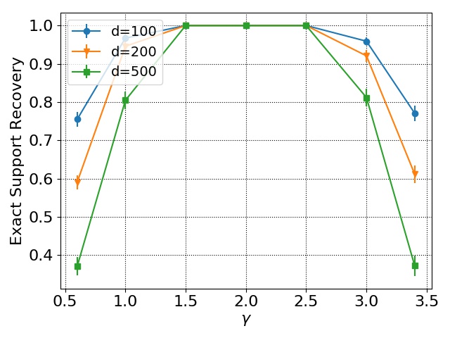
(a) Recovery of $S$ versus $\gamma$

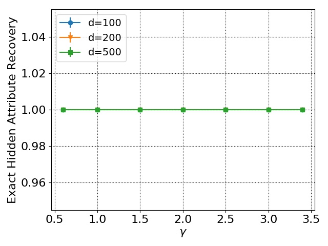
(b) Recovery of $\mathbf{Z}^{*}$ versus $\gamma$

Figure 3: Left: Exact support recovery of $w^{*}$ across $30$ runs. Right: Exact hidden attribute recovery of $\mathbf{Z}*$ across $30$ runs. The true value of $\gamma$ is $2$.

Our method requires a known value of bias parameter $\gamma$ in our analysis. However, in practice, we observe that even a rough estimate (up to $\pm 25\%$) works pretty well. We conducted computational experiments with a range of values of $\gamma$ and the reported results are averaged across $30$ independent runs. The performance measures used here are the same as in Section 5 (See Appendix M for details). Figure 3(a) shows the quality of support recovery for different values of $\gamma$ and Figure 3(b) shows the quality of recovering the hidden attributes for different values of $\gamma$. Note how both the curves show $100\%$ correct recovery for a wide range of $\gamma$. These experiments show that prior knowledge of the exact value of $\gamma$ is not necessary for our method.

Appendix K Alternate Optimization Algorithm for Solving Optimization Problem (6)

We use the following alternate optimization algorithm to solve optimization problem (6) in our computational experiments.

  Input: Data samples $(\mathbf{X},\mathbf{y})$, amount of bias $\gamma$

  Output: $\tilde{w},\mathbf{Z}$

  $\mathbf{Z}_{0}\leftarrow\mathbf{I}_{n+1\times n+1}$

  $\mathbf{z}_{0}\leftarrow\mathbf{Z}_{0}(2:n+1,1)$

  for $t=1,2,\cdots$ until $\mathbf{Z}_{t-1}=\mathbf{Z}_{t}$ do

      $\tilde{w}_{t}\leftarrow\arg\min_{w}\frac{1}{n}(\mathbf{X}w+\gamma\mathbf{z}_{t-1}-\mathbf{y})^{\intercal}(\mathbf{X}w+\gamma\mathbf{z}_{t-1}-\mathbf{y})+\lambda_{n}\|w\|_{1}$

$\mathbf{M}(\tilde{w}_{t})\leftarrow\begin{bmatrix}\frac{1}{n}\|\mathbf{X}\tilde{w}_{t}-\mathbf{y}\|_{2}^{2}&\frac{\gamma}{n}(\mathbf{X}\tilde{w}_{t}-\mathbf{y})^{\intercal}\\ \frac{\gamma}{n}(\mathbf{X}\tilde{w}_{t}-\mathbf{y})^{\intercal}&\frac{\gamma^{2}}{n}\mathbf{I}_{n\times n}\end{bmatrix}$

$\mathbf{Z}_{t}\leftarrow\arg\min_{\mathbf{Z}}{{\rm{trace}}(\mathbf{M}(\tilde{w}_{t})\mathbf{Z})}$, such that ${\rm{diag}}(\mathbf{Z})=\mathbf{1}$, $\mathbf{Z}\succeq\mathbf{0}_{n+1\times n+1}$

$\mathbf{z}_{t}\leftarrow\mathbf{Z}_{t}(2:n+1,1)$

  end for

  $\tilde{w}\leftarrow\tilde{w}_{t},\;\;\mathbf{Z}\leftarrow\mathbf{Z}_{t}$

Algorithm 1 Alternate Optimization Algorithm for our problem

Recall from equation (5) that

$$\begin{split}\mathbf{Z}\triangleq\begin{bmatrix}1&\mathbf{z}^{\intercal}\\ \mathbf{z}&\mathbf{z}\mathbf{z}^{\intercal}\end{bmatrix}.\end{split}$$ (52)

Thus, we can read $\mathbf{z}$ from $\mathbf{Z}$ by considering its first column and skipping the first entry. We denote this as $\mathbf{z}=\mathbf{Z}(2:n+1,1)$. We use a similar notation in Algorithm 1 to assign values to vectors $\mathbf{z}_{0}$ and $\mathbf{z}_{t}$ from matrices $\mathbf{Z}_{0}$ and $\mathbf{Z}_{t}$ respectively.

We will show that if Algorithm 1 converges then it converges to the optimal solution of optimization problem (6). To do this, consider

$$\begin{split}f_{1}(w,\mathbf{Z})&=\frac{1}{n}(\mathbf{X}w+\gamma\mathbf{z}_{t-1}-\mathbf{y})^{\intercal}(\mathbf{X}w+\gamma\mathbf{z}_{t-1}-\mathbf{y})\\ f_{2}(w)&=\lambda_{n}\|w\|_{1}\;.\end{split}$$ (53)

Note that $f_{2}(w)$ is not differentiable. Let $g(\mathbf{Z})\triangleq-{\rm{eig}}_{\min}(\mathbf{Z})$ and $h_{i}(\mathbf{Z})\triangleq\mathbf{Z}_{ii}-1,\forall i\in[n+1]$. Observe that $g(\mathbf{Z})\leq 0$ and $h_{i}(\mathbf{Z})=0,\forall i\in[n+1]$ denote the constraints $\mathbf{Z}\succeq\mathbf{0}_{n+1\times n+1}$ and ${\rm{diag}}(\mathbf{Z})=\mathbf{1}$ respectively. We define $\frac{\partial{f_{2}(w)}}{\partial{w}}$ as the sub-differential set for $f_{2}(w)$ and $f_{2}^{\prime}(w)\in\frac{\partial{f_{2}(w)}}{\partial{w}}$ is an element of the sub-differential set $\frac{\partial{f_{2}(w)}}{\partial{w}}$. Observe that $f_{1}(w,\mathbf{Z})+f_{2}(w)$, $g(\mathbf{Z})$ and $h_{i}(\mathbf{Z})$ are convex with respect to $w$ and $\mathbf{Z}$ separately but they are not jointly convex. Consider the following optimization problem:

$$\begin{split}\tilde{w},\mathbf{Z}^{*}=\begin{matrix}\arg\min_{w,\mathbf{Z}}&f_{1}(w,\mathbf{Z})+f_{2}(w)&\\ \text{such that}&g(\mathbf{Z})\leq 0&\\ &h_{i}(\mathbf{Z})=0&\forall i\in[n+1]\end{matrix}\end{split}$$ (54)

We have already shown that the solution $\tilde{w},\mathbf{Z}^{*}$ is the unique solution to (54). We propose the following alternate optimization algorithm to solve this problem:

  Output: $w,\mathbf{Z}$

  $\mathbf{Z}_{0}\leftarrow\mathbf{I}_{n+1\times n+1}$

  for $t=1,2\cdots$ until $\mathbf{Z}_{t-1}=\mathbf{Z}_{t}$ do

     

$$w_{t}\leftarrow\arg\min_{w}f_{1}(w,\mathbf{Z}_{t-1})+f_{2}(w)$$ (55)

$$\mathbf{Z}_{t}\leftarrow\begin{matrix}\arg\min_{\mathbf{Z}}&f_{1}(w_{t},\mathbf{Z})&\\ \text{such that}&g(\mathbf{Z})\leq 0&\\ &h_{i}(\mathbf{Z})=0&\forall i\in[n+1]\end{matrix}$$ (56)

  end for

  $w\leftarrow w_{t},\;\;\mathbf{Z}\leftarrow\mathbf{Z}_{t}$

Algorithm 2 Alternate Optimization Algorithm

We will prove the following proposition:

Proposition 1.

If Algorithm 2 converges, then $w=\tilde{w}$ and $\mathbf{Z}=\mathbf{Z}^{*}$.

Proof.

We start by writing the KKT conditions for optimization problem (54).

1. Stationarity conditions: $\frac{\partial{f_{1}(\tilde{w},\mathbf{Z}^{*})}}{\partial{w}}+f_{2}^{\prime}(\tilde{w})=0$ and $\frac{\partial{f_{1}(\tilde{w},\mathbf{Z}^{*})}}{\partial{\mathbf{Z}}}+r\frac{\partial{g(\mathbf{Z}^{*})}}{\partial{\mathbf{Z}}}+\sum_{i=1}^{n+1}s_{i}\frac{\partial{h_{i}(\mathbf{Z}^{*})}}{\partial{\mathbf{Z}}}=0$.

2. Complementary slackness condition: $rg(\mathbf{Z}^{*})=0$.

3. Primal feasibility condition: $g(\mathbf{Z}^{*})\leq 0$ and $h_{i}(\mathbf{Z}^{*})=0,\forall i\in[n+1]$.

4. Dual feasibility condition: $r\geq 0$.

Any optimal solution to optimization problem (54) must satisfy the above KKT conditions. Next, we write the KKT conditions for (55) at convergence, i.e., at $\mathbf{Z}_{t}=\mathbf{Z}_{t-1}$:

1. Stationarity condition: $\frac{\partial{f(w_{t},\mathbf{Z}_{t})}}{\partial{w}}+f_{2}^{\prime}(w_{t})=0$

Similarly, we write the KKT conditions for (56) at convergence, i.e., at $\mathbf{Z}_{t}=\mathbf{Z}_{t-1}$:

1. Stationarity conditions: $\frac{\partial{f_{1}(w_{t},\mathbf{Z}_{t})}}{\partial{\mathbf{Z}}}+t\frac{\partial{g(\mathbf{Z}_{t})}}{\partial{\mathbf{Z}}}+\sum_{i=1}^{n+1}u_{i}\frac{\partial{h_{i}(\mathbf{Z}_{t})}}{\partial{\mathbf{Z}}}=0$.

2. Complementary slackness condition: $tg(\mathbf{Z}_{t})=0$.

3. Primal feasibility condition: $g(\mathbf{Z}_{t})\leq 0$ and $h_{i}(\mathbf{Z}_{t})=0,\forall i\in[n+1]$.

4. Dual feasibility condition: $t\geq 0$.

Combining the KKT conditions at $w_{t},\mathbf{Z}_{t}$ for (55) and (56) and taking $r=t$ and $s_{i}=u_{i},\forall i\in[n+1]$, we see that all KKT conditions of (54) are satisfied by $w_{t},\mathbf{Z}_{t}$. Since the solution to (54) is unique, it follows that $w=\tilde{w}$ and $\mathbf{Z}=\mathbf{Z}^{*}$. ∎

Appendix L Our Assumptions Hold for Finite Samples

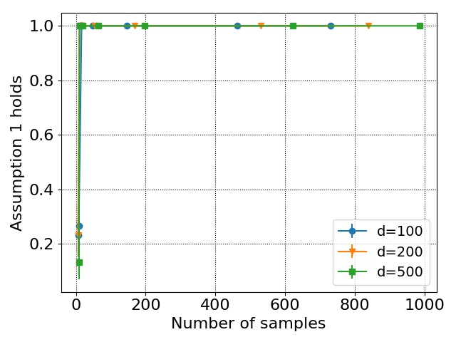
(a) Positive Definiteness against number of samples

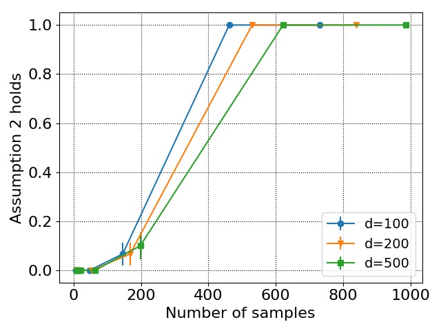
(b) Mutual Incoherence against number of samples

Figure 4: Left: Positive Definiteness Assumption 1 with varying number of samples for $d=100,200$ and $500$, Right: Mutual Incoherence Assumption 2 with varying number of samples for $d=100,200$ and $d=500$.

Figure 4 shows how our assumptions hold (averaged across 30 independent runs) in the finite sample regime with varying number of samples when $X$ is drawn from a standard normal distribution. We notice that for a fixed $s$, Assumption 1 is easier to hold (i.e., $n=\Omega(s+\log d)$) than Assumption 2 (i.e., $n=\Omega(s^{3}\log d)$). Eventually, both assumptions hold as the number of samples increases.

Appendix M Details of Experimental Validation

In this section, we validate our theoretical results by conducting computational experiments on synthetic data. We will show that for a fixed $s$, we need $n=10^{\beta}\log d$ samples for recovering the exact support of $w^{*}$ and exact hidden attributes $\mathbf{Z}^{*}$, where $\beta\equiv\beta(s,C_{\min},\alpha,\sigma,\Sigma,\rho,\gamma,k)$ is a control parameter which is independent of $d$.

Data Generation.

For $d=100,200$ and $500$, we draw $\mathbf{X}\in^{n\times d}$ from a standard Gaussian distribution by varying $n$ as $10^{\beta}\log d$ for a control parameter $\beta$. The $s=10$ non-zero entries of true parameter $w^{*}\in^{d}$ are chosen uniformly at random between $[-1,1]$. Every non-zero entry in $w^{*}$ is changed to at least $0.75$ to make sure that it is not too close to $0$. The independent noise $\mathbf{e}\in^{n}$ is drawn from a zero mean Gaussian distribution with standard deviation $\frac{k}{\sqrt{\log n}}$ for $k=0.15$. The estimate of the bias $\gamma\in_{>0}$ is kept at $2$. Regarding the hidden attribute $\mathbf{z}^{*}\in\{-1,1\}^{n}$, we set $\frac{n}{2}$ entries as $+1$ and the rest as $-1$. The response $\mathbf{y}\in^{n}$ is generated according to (1). This process is repeated $30$ times and the reported results are averaged across these $30$ independent runs.

Choice of Regularizer and Solution.

According to Theorem 1, the regularizer $\lambda_{n}$ is chosen to be equal to $\frac{128\rho k}{\alpha}\frac{\sqrt{\log d}}{n}$. We solve optimization problem (6) by using an alternate optimization algorithm that converges to the optimal solution (See Appendix K for details).

Measure of Performance.

The performance is measured by comparing the recovered solutions $\tilde{w}$ and $\mathbf{Z}$ with the true parameters $w^{*}$ and $\mathbf{Z}^{*}$. The quality of $\tilde{w}$ is measured by comparing its support to the support $S$ of the true parameter $w^{*}$ by computing the Jaccard index $J(S,\hat{S})$, where $\hat{S}$ is the support of $\tilde{w}$, i.e., $\hat{S}=\{i|\tilde{w}_{i}\neq 0,i\in[d]\}$. The average of $J(S,\hat{S})$ across 30 independent runs is plotted against the number of samples $n$ (See Figure 2(a), 2(b)). Similarly, the quality of $\mathbf{Z}$ is measured by the indicator variable $I(\mathbf{Z},\mathbf{Z}^{*})$. The average of $I(\mathbf{Z},\mathbf{Z}^{*})$ across 30 independent runs is plotted against the number of samples $n$ (See Figure 2(c), 2(d)). The Jaccard index $J(S,\hat{S})$ and indicator variable $I(\mathbf{Z},\mathbf{Z}^{*})$ are defined as follows:

$$\begin{split}J(S,\hat{S})\triangleq\frac{|S\cap\hat{S}|}{|S\cup\hat{S}|},\;\;\;I(\mathbf{Z},\mathbf{Z}^{*})\triangleq\begin{cases}0,\;\rm{if}\;\mathbf{Z}\neq\mathbf{Z}^{*}\\ 1\;\rm{if}\;\mathbf{Z}=\mathbf{Z}^{*}\end{cases}\end{split}$$

Observation.

Figure 2(a) shows the Jaccard index of support recovery with varying number of samples. We see that our method recovers the true support for all three values of $d$ as we increase number of samples. Also, notice how all three curves line up perfectly in Figure 2(b) when we plot the support recovery with respect to the control parameter $\beta=\log\frac{n}{\log d}$. This validates our theoretical results. Similarly, Figure 2(c) shows exact recovery of the hidden attribute with varying number of samples. We again see that as the number of samples increase, our recovered hidden attributes are 100% correct. Again, the three different curves for different values of $d$ line up nicely when plotted against $\beta$. Interestingly, a small percentage of our experiments recover the hidden attributes exactly for small number of samples ($<20$). We believe that this can be ascribed to $\mathbf{Z}^{*}$ having small dimensions and thus becoming relatively easier to recover. On a more practical point of view, once hidden attributes are identified for each sample point, the associated bias (for and against) can be duly removed from the model.

Appendix N Optimization Problem (6) is Non-Convex

Before we begin the proof of non-convexity of (6), we note that optimization (6) is stated for a fixed $\mathbf{X}$. However, since the entries in $\mathbf{X}$ are drawn from a sub-Gaussian distribution, matrix $\mathbf{X}$ can potentially realize any real matrix in ^n×d. In particular, we are interested in a problem where $\exists i,k\in[d]$ such that $\sum_{l=1}^{n}\mathbf{X}_{li}^{2}-\mathbf{X}_{ki}$ is non-zero. Since $\mathbf{X}$ can be any real matrix in ^n×d, this is not a strong assumption. With this assumption in mind, we present the following lemma.

Lemma 13.

The optimization problem (6) defined on a convex set $C$, is non-convex.

Proof.

As defined in (6), we define the domain for optimization problem on a convex set $C=\{(w,\mathbf{Z})\mid w\in^{d},{\rm{diag}}(\mathbf{Z})=\mathbf{1},\mathbf{Z}\succeq\mathbf{0}_{n+1\times n+1}\}$. It should be noted that $C$ is a convex set and we will show that the non-convexity of the problem comes from the objective function. We are solving the following optimization problem:

$$\begin{split}\begin{matrix}\min_{(w,\mathbf{Z})\in C}&\langle\mathbf{M}(w),\mathbf{Z}\rangle+\lambda_{n}\|w\|_{1}\\ \end{matrix}\,,\end{split}$$ (57)

It suffices to show that $f(w,\mathbf{Z})=\langle\mathbf{M}(w),\mathbf{Z}\rangle$ is non-convex function. To that end, we will construct a setting of $(w,\mathbf{Z})\in C$ and $(\bar{w},\bar{\mathbf{Z}})\in C$ such that the first order condition for convexity fails to hold, i.e,

$$\begin{split}f(w,\mathbf{Z})-f(\bar{w},\bar{\mathbf{Z}})<\langle\frac{\partial{f(\bar{w},\bar{\mathbf{Z}})}}{\partial{w}},(w-\bar{w})\rangle+\langle\frac{\partial{f(\bar{w},\bar{\mathbf{Z}})}}{\partial{\mathbf{Z}}},\mathbf{Z}-\bar{\mathbf{Z}}\rangle.\end{split}$$ (58)

First notice that,

$$\begin{split}\frac{\partial{f(\bar{w},\bar{\mathbf{Z}})}}{\partial{w}}=\sum_{ij}\bar{\mathbf{Z}}_{ij}\frac{\partial{\mathbf{M}_{ij}(\bar{w})}}{\partial{w}},\;\;\;\frac{\partial{f(\bar{w},\bar{\mathbf{Z}})}}{\partial{\mathbf{Z}}}=\mathbf{M}(\bar{w})\end{split}$$

Recall from equation (5) that,

$$\begin{split}&l(w)\triangleq\frac{1}{n}(\mathbf{X}w-\mathbf{y})^{\intercal}(\mathbf{X}w-\mathbf{y}),\;\;\mathbf{M}(w)\triangleq\begin{bmatrix}l(w)&\frac{\gamma}{n}(\mathbf{X}w-\mathbf{y})^{\intercal}\\ \frac{\gamma}{n}(\mathbf{X}w-\mathbf{y})&\frac{\gamma^{2}}{n}\mathbf{I}_{n\times n}\end{bmatrix},\end{split}$$ (59)

Then $\frac{\partial{f(\bar{w},\bar{\mathbf{Z}})}}{\partial{w}}$ can be simplified as:

$$\begin{split}\frac{\partial{f(\bar{w},\bar{\mathbf{Z}})}}{\partial{w}}=\frac{2}{n}(\mathbf{X}^{\intercal}\mathbf{X}\bar{w}-\mathbf{X}^{\intercal}\mathbf{y}+\mathbf{X}^{\intercal}\bar{\mathbf{z}}),\end{split}$$ (60)

where $\bar{\mathbf{z}}\in^{n}$ denotes the first column of $\bar{\mathbf{Z}}$ after skipping the first entry.

We provide the following construction for $(w,\mathbf{Z})\in C$ and $(\bar{w},\bar{\mathbf{Z}})\in C$. We take $w\in\{0,\beta\}^{d}$ such that $w_{k}=0,\forall k\neq i$ and $w_{i}=\beta$ where $\beta\in$. Similarly, $\bar{w}\in\{0,\beta\}^{d}$ such that $\bar{w}_{k}=0,\forall k\neq i$ and $\bar{w}_{i}=-\beta$. Since $w\in^{d}$, such a setting exists for a non-zero $\beta$. Furthermore, we take $\mathbf{Z}=\mathbf{I}_{n+1\times n+1}$ and $\bar{\mathbf{Z}}\in\{0,1\}^{n+1\times n+1}$ such that $\bar{\mathbf{Z}}_{ii}=1,\forall i\in[n+1]$ and $\bar{\mathbf{Z}}_{1(k+1)}=1,\bar{\mathbf{Z}}_{(k+1)1}=1$. Now, we can compute the following quantities:

$$\begin{split}\langle\mathbf{M}(w),\mathbf{Z}\rangle&=l(w)+\gamma^{2}=\frac{1}{n}\sum_{l=1}^{n}(\mathbf{X}_{li}w_{i}-y_{l})^{2}+\gamma^{2}\\ \langle\mathbf{M}(\bar{w}),\bar{\mathbf{Z}}\rangle&=l(\bar{w})+\gamma^{2}-\frac{2\gamma}{n}(\mathbf{X}_{ki}\bar{w}_{i}-y_{k})=\frac{1}{n}\sum_{l=1}^{n}(\mathbf{X}_{li}\bar{w}_{i}-y_{l})^{2}+\gamma^{2}+\frac{2\gamma}{n}(\mathbf{X}_{ki}\bar{w}_{i}-y_{k})\\ \langle\mathbf{M}(\bar{w}),\mathbf{Z}-\bar{\mathbf{Z}}\rangle&=-\frac{2\gamma}{n}(\mathbf{X}_{ki}\bar{w}_{i}-y_{k})\\ \langle\frac{\partial{f(\bar{w},\bar{\mathbf{Z}})}}{\partial{w}},w-\bar{w}\rangle&=\frac{2}{n}((w_{i}\bar{w}_{i}-\bar{w}_{i}^{2})\sum_{l=1}^{n}\mathbf{X}_{li}^{2}+(-w_{i}+\bar{w}_{i})\sum_{l=1}^{n}\mathbf{X}_{li}\mathbf{y}_{l}+(w_{i}-\bar{w}_{i})\mathbf{X}_{ki})\end{split}$$ (61)

Substituting $w_{i}=\beta$ and $\bar{w}_{i}=-\beta$, we get

$$\begin{split}l(w)-l(\bar{w})&=-\frac{4\beta}{n}\sum_{l=1}^{n}\mathbf{X}_{li}\mathbf{y}_{l}\\ \langle\frac{\partial{f(\bar{w},\bar{\mathbf{Z}})}}{\partial{w}},w-\bar{w}\rangle&=-\frac{4\beta}{n}\sum_{l=1}^{n}\mathbf{X}_{li}^{2}-\frac{4\beta}{n}\sum_{l=1}^{n}\mathbf{X}_{li}\mathbf{y}_{l}+\frac{4\beta}{n}\mathbf{X}_{ki}\end{split}$$ (62)

Clearly,

$$\begin{split}\langle\mathbf{M}(w),\mathbf{Z}\rangle-\langle\mathbf{M}(\bar{w}),\bar{\mathbf{Z}}\rangle&=-\frac{4\beta}{n}\sum_{l=1}^{n}\mathbf{X}_{li}\mathbf{y}_{l}-\frac{2\gamma}{n}(\mathbf{X}_{ki}\bar{w}_{i}-y_{k})\\ \langle\mathbf{M}(\bar{w}),\mathbf{Z}-\bar{\mathbf{Z}}\rangle+\langle\frac{\partial{f(\bar{w},\bar{\mathbf{Z}})}}{\partial{w}},w-\bar{w}\rangle&=-\frac{2\gamma}{n}(\mathbf{X}_{ki}\bar{w}_{i}-y_{k})-\frac{4\beta}{n}\sum_{l=1}^{n}\mathbf{X}_{li}^{2}-\frac{4\beta}{n}\sum_{l=1}^{n}\mathbf{X}_{li}\mathbf{y}_{l}+\frac{4\beta}{n}\mathbf{X}_{ki}\end{split}$$ (63)

It follows that

$$\begin{split}\langle\mathbf{M}(w),\mathbf{Z}\rangle-\langle\mathbf{M}(\bar{w}),\bar{\mathbf{Z}}\rangle-\langle\mathbf{M}(\bar{w}),\mathbf{Z}-\bar{\mathbf{Z}}\rangle-\langle\frac{\partial{f(\bar{w},\bar{\mathbf{Z}})}}{\partial{w}},w-\bar{w}\rangle=\beta(\frac{4}{n}\sum_{l=1}^{n}\mathbf{X}_{li}^{2}-\frac{4}{n}\mathbf{X}_{ki})\end{split}$$ (64)

As $\sum_{l=1}^{n}\mathbf{X}_{li}^{2}-\mathbf{X}_{ki}$ is assumed to be non-zero, it is easy to see that LHS of equation (64)can be made greater than or less than $0$ by simply choosing appropriate $\beta\in$. Thus, optimization problem (6) is non-convex. ∎

Appendix O Real World Experiment

We show applicability of our method by conducting experiments on Communities and Crime Data Set [Redmond(2002)] and Student Performance Data Set [Cortez(2008)].

O.1 Communities and Crime Data Set

This data set contains $1994$ samples with $122$ predictors which might have plausible connection to crime, and the attribute to be predicted (Per Capita Violent Crimes). In the preprocessing step, any predictors with missing values are removed and all the predictors and the attribute to be predicted are standardized to have zero mean and unit standard deviation. The preprocessed dataset contains $d=100$ predictors and $n=1994$ samples.

The optimization problem (6) is solved for $\lambda_{n}=0.15$ and $\gamma$ is chosen to be $\frac{\max(\mathbf{y})-\min(\mathbf{y})}{2}$. As the problem is invex, any algorithm which converges to a stationary point can be used to solve the problem. We used an alternate optimization algorithm (See Appendix K) which converges to an optimal solution.

Main results.

Based on the support (non-zero entries) in the recovered $w$, we found that the following are the most important predictors of Per Capita Violent Crimes:

1. PctHousNoPhone: percentage of occupied housing units without phone

2. PctNotHSGrad: percentage of people 25 and over that are not high school graduates

3. PctLess9thGrade: percentage of people 25 and over with less than a 9th grade education

4. RentLowQ: rental housing - lower quartile rent

We also recovered the hidden sensitive attribute with $816$ instances of positive bias ($z=+1$) with mean crime rate $0.8002$ and $1178$ instances of negative bias ($z=-1$) with mean crime rate $-0.5543$. By plotting data with two of the most important predictors (PctHousNoPhone, PctNotHSGrad), we clearly see the existence of two groups (Figure 5). Our Mean Squared Error (MSE) is $0.0265$. [Chzhen et al.(2020)] can be checked for comparison with other state-of-the-art methods ($12$ methods of $3$ different types) where only the Kernel Regularized Least Square method (MSE=$0.024\pm 0.003$) and the Random Forests method (MSE=$0.020\pm 0.002$) perform better than our method in terms of MSE but suffer heavily in terms of fairness. Other methods incur MSE in the range between $0.028\pm 0.003$ to $0.041\pm 0.004$.

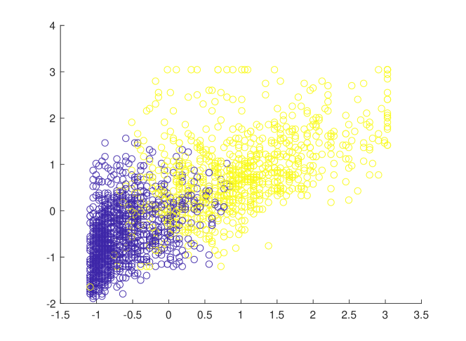
Figure 5: Clusters in Communities and Crime Dataset

O.2 Student Performance Data Set

This data set contains $649$ samples with $33$ demographic, social and school predictors and the attribute to be predicted (grade in the Portuguese Language course). The data set contains some categorical variables which are converted to numerical variables using dummy encoding (thus increasing the number of predictors). Two columns containing partial grades were removed from the data set. In the preprocessing step, all the predictors and the attribute to be predicted are standardized to have zero mean and unit standard deviation. The preprocessed dataset contains $d=39$ predictors and $n=649$ samples.

Similar to subsection O.1, the optimization problem (6) is solved for $\lambda_{n}=0.15$ and $\gamma=\frac{\max(\mathbf{y})-\min(\mathbf{y})}{2}$.

Main results.

The following are the most important predictors of grades in the Portuguese Language course:

1. school: student’s school

2. failures: number of past class failures

3. higher: wants to take higher education

We also recovered the hidden sensitive attribute with $420$ instances of positive bias ($z=+1$) with mean grade $0.2305$ and $229$ instances of negative bias ($z=-1$) with mean grade $-0.4227$. Our Mean Squared Error (MSE) is $0.0494$. [Chzhen et al.(2020)] can be checked for comparison with other state-of-the-art methods ($12$ methods of $3$ different types) where none of the methods performs better than our method in terms of MSE (range between $3.59\pm 0.39$ to $5.62\pm 0.52$).

O.3 Discussion.

While our analysis identifies two groups with bias in both data sets, it cannot only be attributed to the most important recovered predictors. Recall the “red-lining” effect [Calders(2010)] where there might be other correlated predictors which can facilitate indirect discrimination. For example: in the Communities and Crime data set, annual income could be correlated with PctHousNoPhone and similarly in the Student Performance data set, parents’ educational qualification could be correlated with student’s willingness to go for higher education. Our analysis does not ignore such factors. In fact, even after taking the red-lining effect into the consideration, our method is able to identify two groups with bias.

References

- [Agarwal et al.(2018)] Agarwal, A., Beygelzimer, A., Dudík, M., Langford, J., and Wallach, H. A reductions approach to fair classification. International Conference on Machine Learning, 2018.
- [Agarwal et al.(2019)] Agarwal, A., Dudík, M., and Wu, Z. S. Fair regression: Quantitative definitions and reduction-based algorithms. International Conference on Machine Learning, 2019.
- [Backurs et al.(2019)] Backurs, A., Indyk, P., Onak, K., Schieber, B., Vakilian, A., and Wagner, T. Scalable fair clustering. In International Conference on Machine Learning, pp. 405–413. PMLR, 2019.
- [Ben-Israel & Mond(1986)] Ben-Israel, A. and Mond, B. What is invexity? The ANZIAM Journal, 28(1):1–9, 1986.
- [Bera et al.(2019)] Bera, S. K., Chakrabarty, D., Flores, N. J., and Negahbani, M. Fair algorithms for clustering. Neural Information Processing Systems, 2019.
- [Berk et al.(2017)] Berk, R., Heidari, H., Jabbari, S., Joseph, M., Kearns, M., Morgenstern, J., Neel, S., and Roth, A. A convex framework for fair regression. ACM International Conference on Knowledge Discovery and Data Mining, Workshop on Fairness, Accountability, and Transparency in Machine Learning, 2017.
- [Brennan et al.(2009)] Brennan, T., Dieterich, W., and Ehret, B. Evaluating the predictive validity of the compas risk and needs assessment system. Criminal Justice and Behavior, 36(1):21–40, 2009.
- [Calders et al.(2013)] Calders, T., Karim, A., Kamiran, F., Ali, W., and Zhang, X. Controlling attribute effect in linear regression. 2013 IEEE 13th international conference on data mining, pp. 71–80, 2013.
- [Chen et al.(2019)] Chen, X., Fain, B., Lyu, L., and Munagala, K. Proportionally fair clustering. In International Conference on Machine Learning, pp. 1032–1041. PMLR, 2019.
- [Chierichetti et al.(2017)] Chierichetti, F., Kumar, R., Lattanzi, S., and Vassilvitskii, S. Fair clustering through fairlets. Neural Information Processing Systems, 2017.
- [Chzhen et al.(2020)] Chzhen, E., Denis, C., Hebiri, M., Oneto, L., and Pontil, M. Fair regression with wasserstein barycenters. Neural Information Processing Systems, 2020.
- [Corbett-Davies et al.(2017)] Corbett-Davies, S., Pierson, E., Feller, A., Goel, S., and Huq, A. Algorithmic decision making and the cost of fairness. In Proceedings of the 23rd acm sigkdd international conference on knowledge discovery and data mining, pp. 797–806, 2017.
- [Daneshmand et al.(2014)] Daneshmand, H., Gomez-Rodriguez, M., Song, L., and Schoelkopf, B. Estimating Diffusion Network Structures: Recovery Conditions, Sample Complexity & Soft-Thresholding Algorithm. In International Conference on Machine Learning, pp. 793–801, 2014.
- [Donini et al.(2018)] Donini, M., Oneto, L., Ben-David, S., Shawe-Taylor, J. S., and Pontil, M. Empirical risk minimization under fairness constraints. pp. 2791–2801, 2018.
- [Dwork et al.(2012)] Dwork, C., Hardt, M., Pitassi, T., Reingold, O., and Zemel, R. Fairness through awareness. In Proceedings of the 3rd innovations in theoretical computer science conference, pp. 214–226, 2012.
- [Feldman et al.(2015)] Feldman, M., Friedler, S. A., Moeller, J., Scheidegger, C., and Venkatasubramanian, S. Certifying and removing disparate impact. In proceedings of the 21th ACM SIGKDD international conference on knowledge discovery and data mining, pp. 259–268, 2015.
- [Hanson(1981)] Hanson, M. A. On sufficiency of the kuhn-tucker conditions. Journal of Mathematical Analysis and Applications, 80(2):545–550, 1981.
- [Hardt et al.(2016)] Hardt, M., Price, E., and Srebro, N. Equality of opportunity in supervised learning. In Advances in neural information processing systems, pp. 3315–3323, 2016.
- [Haynsworth(1968)] Haynsworth, E. V. Determination of the inertia of a partitioned hermitian matrix. Linear algebra and its applications, 1(1):73–81, 1968.
- [Hoffman et al.(2018)] Hoffman, M., Kahn, L. B., and Li, D. Discretion in hiring. The Quarterly Journal of Economics, 133(2):765–800, 2018.
- [Horn & Johnson(2012)] Horn, R. A. and Johnson, C. R. Matrix analysis. Cambridge university press, 2012.
- [Hsu et al.(2012)] Hsu, D., Kakade, S., Zhang, T., et al. A tail inequality for quadratic forms of subgaussian random vectors. Electronic Communications in Probability, 17, 2012.
- [Huang & Vishnoi(2019)] Huang, L. and Vishnoi, N. K. Stable and fair classification. International Conference on Machine Learning, 2019.
- [Huang et al.(2019)] Huang, L., Jiang, S. H.-C., and Vishnoi, N. K. Coresets for clustering with fairness constraints. Neural Information Processing Systems, 2019.
- [Kleinberg et al.(2017)] Kleinberg, J., Mullainathan, S., and Raghavan, M. Inherent trade-offs in the fair determination of risk scores. Innovations in Theoretical Computer Science, 2017.
- [Kleinberg et al.(2018)] Kleinberg, J., Lakkaraju, H., Leskovec, J., Ludwig, J., and Mullainathan, S. Human decisions and machine predictions. The quarterly journal of economics, 133(1):237–293, 2018.
- [Knutson & Tao(2001)] Knutson, A. and Tao, T. Honeycombs and sums of hermitian matrices. Notices Amer. Math. Soc, 48(2), 2001.
- [Pedreshi et al.(2008)] Pedreshi, D., Ruggieri, S., and Turini, F. Discrimination-aware data mining. In Proceedings of the 14th ACM SIGKDD international conference on Knowledge discovery and data mining, pp. 560–568, 2008.
- [Pleiss et al.(2017)] Pleiss, G., Raghavan, M., Wu, F., Kleinberg, J., and Weinberger, K. Q. On fairness and calibration. Neural Information Processing Systems, 2017.
- [Ravikumar et al.(2007)] Ravikumar, P., Liu, H., Lafferty, J., and Wasserman, L. Spam: Sparse Additive Models. In Proceedings of the 20th International Conference on Neural Information Processing Systems, pp. 1201–1208. Curran Associates Inc., 2007.
- [Ravikumar et al.(2010)] Ravikumar, P., Wainwright, M. J., Lafferty, J. D., et al. High-dimensional ising model selection using l1-regularized logistic regression. The Annals of Statistics, 38(3):1287–1319, 2010.
- [Ravikumar et al.(2011)] Ravikumar, P., Wainwright, M. J., Raskutti, G., Yu, B., et al. High-dimensional covariance estimation by minimizing l1-penalized log-determinant divergence. Electronic Journal of Statistics, 5:935–980, 2011.
- [Subrahmanian & Kumar(2017)] Subrahmanian, V. and Kumar, S. Predicting human behavior: The next frontiers. Science, 355(6324):489–489, 2017.
- [Vershynin(2012)] Vershynin, R. How close is the sample covariance matrix to the actual covariance matrix? Journal of Theoretical Probability, 25(3):655–686, 2012.
- [Wainwright(2009)] Wainwright, M. J. Sharp thresholds for high-dimensional and noisy sparsity recovery using l1-constrained quadratic programming (lasso). IEEE transactions on information theory, 55(5):2183–2202, 2009.
- [Wainwright(2019)] Wainwright, M. J. High-dimensional statistics: A non-asymptotic viewpoint, volume 48. Cambridge University Press, 2019.
- [Zafar et al.(2019)] Zafar, M. B., Valera, I., Gomez-Rodriguez, M., and Gummadi, K. P. Fairness constraints: A flexible approach for fair classification. Journal of Machine Learning Research, 20(75):1–42, 2019.
- [Zemel et al.(2013)] Zemel, R., Wu, Y., Swersky, K., Pitassi, T., and Dwork, C. Learning fair representations. In International Conference on Machine Learning, pp. 325–333, 2013.
- [Zhao & Gordon(2019)] Zhao, H. and Gordon, G. J. Inherent tradeoffs in learning fair representations. Neural Information Processing Systems, 2019.
- [Zliobaite(2015)] Zliobaite, I. On the relation between accuracy and fairness in binary classification. Interna- tional Conference on Machine Learning, Workshop on Fairness, Accountability, and Transparency in Machine Learning, 2015.
- [Calders(2013)] Calders, Toon and Karim, Asim and Kamiran, Faisal and Ali, Wasif and Zhang, Xiangliang Controlling attribute effect in linear regression. IEEE 13th international conference on data mining, 2013.
- [Berk(2017)] Berk, Richard and Heidari, Hoda and Jabbari, Shahin and Joseph, Matthew and Kearns, Michael and Morgenstern, Jamie and Neel, Seth and Roth, Aaron A convex framework for fair regression. Fairness, Accountability, and Transparency in Machine Learning, 2017.
- [Agarwal(2019)] Agarwal, Alekh and Dudik, Miroslav and Wu, Zhiwei Steven Fair regression: Quantitative definitions and reduction-based algorithms. International Conference on Machine Learning, 2019.
- [Fitzsimons(2019)] Fitzsimons, Jack and Al Ali, AbdulRahman and Osborne, Michael and Roberts, Stephen A general framework for fair regression. Entropy, 2019.
- [Calders(2010)] Calders, Toon and Verwer, Sicco Three naive bayes approaches for discrimination-free classification. Data Mining and Knowledge Discovery, 2010.
- [Billionnet(2010)] Billionnet, Alain and Elloumi, Sourour Using a mixed integer quadratic programming solver for the unconstrained quadratic 0-1 problem. Mathematical Programming, 2007.
- [Redmond(2002)] Redmond, Michael and Baveja, Alok A data-driven software tool for enabling cooperative information sharing among police departments. European Journal of Operational Research, 2002.
- [Cortez(2008)] Cortez, Paulo and Silva, Alice Maria Gonçalves Using data mining to predict secondary school student performance. EUROSIS-ETI, 2008.