Near-Optimal Randomized Exploration for Tabular Markov Decision Processes

Abstract

We study algorithms using randomized value functions for exploration in reinforcement learning. This type of algorithms enjoys appealing empirical performance. We show that when we use 1) a single random seed in each episode, and 2) a Bernstein-type magnitude of noise, we obtain a worst-case $\widetilde{O}\left(H\sqrt{SAT}\right)$ regret bound for episodic time-inhomogeneous Markov Decision Process where $S$ is the size of state space, $A$ is the size of action space, $H$ is the planning horizon and $T$ is the number of interactions. This bound polynomially improves all existing bounds for algorithms based on randomized value functions, and for the first time, matches the $\Omega\left(H\sqrt{SAT}\right)$ lower bound up to logarithmic factors. Our result highlights that randomized exploration can be near-optimal, which was previously achieved only by optimistic algorithms. To achieve the desired result, we develop 1) a new clipping operation to ensure both the probability of being optimistic and the probability of being pessimistic are lower bounded by a constant, and 2) a new recursive formula for the absolute value of estimation errors to analyze the regret.

1 Introduction

This paper concerns learning in tabular Markov Decision Processes (MDP), arguably the most fundamental model for reinforcement learning (RL). Existing algorithms that achieve the near-optimal minimax $\widetilde{O}\left(H\sqrt{SAT}\right)$ regret bound are based on the principle of Optimism in the face of Uncertainty (OFU), such as upper confidence bound (UCB) (Azar et al., 2017; Zanette and Brunskill, 2019; Dann et al., 2019; Zhang et al., 2020c, a). Here $S$ is the number of states, $A$ is the number of actions, $H$ is the planning horizon, and $T$ is the total number of interactions between the agent and the environment.

Another broad category is algorithms with randomized exploration such as Thompson Sampling (Osband et al., 2013; Agrawal and Jia, 2017a; Osband et al., 2014). These algorithms inject (carefully tuned) random noise to value function to encourage exploration. UCB-type algorithms enjoy well-established theoretical guarantees but suffer from difficult implementation since an upper confidence bound is usually infeasible for many practical models like neural networks. Instead, practitioners prefer randomized exploration such as noisy networks in Fortunato et al. (2018), and algorithms with randomized exploration have been widely used in practice  (Osband et al., 2017; Chapelle and Li, 2011; Burda et al., 2018; Osband et al., 2018). However, how to design randomized exploration algorithms in a principled way and perform randomized exploration optimally is far from clear. While randomized exploration can have great performance in practice, theoretically, the best known worst-case regret bound for algorithms with randomized exploration is $\widetilde{O}\left(H^{2}S\sqrt{AT}\right)$ (Agrawal et al., 2021), which is far worse than that of the UCB-type algorithms. In this paper, we introduce a new randomized exploration algorithm and show it enjoys a near-optimal $\widetilde{O}\left(H\sqrt{SAT}\right)$ worst-case regret bound, thus closing the gap. Our work sheds new light on randomized exploration on both the algorithmic side and the theoretical side.

Our Contributions.

Our contributions are summarized below:

$\bullet$ We propose a new algorithm, Single Seed Randomization (SSR), which incorporates a crucial algorithmic idea: using a single random seed for the entire episode, in contrast to previous methods of randomized exploration which use one seed for each time step. SSR is able to explore more efficiently than previous methods by avoiding having noise at different time steps canceling with each other. Theoretically, we show, thanks to this new idea, if one uses a Hoeffding-type magnitude of noise, SSR achieves an $\widetilde{O}\left(H^{1.5}\sqrt{SAT}\right)$ regret bound, improving upon the best existing result on randomized exploration algorithm (Agrawal et al., 2021).

$\bullet$ We further design a new Bernstein-type magnitude of noise for our algorithm, and achieve an $\widetilde{O}\left(H\sqrt{SAT}\right)$ regret bound, resolving an open problem raised in Agrawal et al. (2021). To our knowledge, this is the first time that a Bernstein-type bound is used in randomized exploration. More importantly, our upper bound matches the $\Omega\left(H\sqrt{SAT}\right)$ minimax lower bound up to logarithmic factors.

We note that our goal is not to show randomized exploration is better than optimistic algorithms (Azar et al., 2017) in the tabular setting. Instead, we aim to provide a solid theoretical understanding of a practically relevant algorithm. Indeed, understanding randomized exploration itself is an important theoretical research direction and has attracted much interest in the community (Agrawal and Goyal, 2012, 2017; Agrawal and Jia, 2017b; Russo, 2019; Zanette et al., 2020; Vaswani et al., 2020; Agrawal et al., 2021; Osband et al., 2013, 2014, 2017, 2018).

Main Challenge and Technical Overview.

Besides the aforementioned algorithmic ideas (single random seed and Bernstein-type magnitude of noise), we also need additional ideas in analysis to prove the desired regret bound. The main challenge is that unlike UCB-type algorithms, the estimated value in algorithm with randomized exploration, is not an upper bound of the true optimal value. This leads to the failure of directly utilizing their analysis, which only need to analyze the one-sided error in estimation. We instead work on the absolute value of the estimation error, whose analysis is more complicated than that for the one-sided error in UCB-type algorithms. Working with absolute value forces us to ensure that both the probability that the estimated value is optimistic and the probability that the estimated value is pessimistic are lower bounded. However, the clipping strategy in existing algorithm cannot maintain pessimism. To tackle with this issue, we develop a new clipping method. Below we list our technical contributions.

1. First, we propose a new clipping strategy to constrain the estimated value function (cf. Eqn. (4)). Previous clipping strategies in (Zanette et al., 2020; Agrawal et al., 2021) are based on uncertainty and can only maintain optimism. Our clipping strategy directly works on the value function, which is similar to those used in UCB-type algorithms (Azar et al., 2017; Jin et al., 2018; Zhang et al., 2020c). Our clipping strategy can maintain both the optimism and pessimism. In addition, the number of times that the clipping is used can still be bounded.

2. Second, we prove that the single seed randomization ensures that the estimated value function can both be optimistic or pessimistic with constant probability at all states and timesteps. This is stronger than previous randomized exploration algorithms that are only shown to be optimistic at the initial state with constant probability. With this property, we can then bound the difference between the optimal value function and estimated value function from both above and below, which results in a bound on its absolute value. See Section 5.1, Appendix C and Appendix D.

3. Third, we prove a novel recursion argument on the absolute value of the policy estimation error. As mentioned in (Agrawal et al., 2021), the recursion in UCB-type algorithms can not be directly utilized because our estimated value function is not a high-probability upper bound of the true optimal value function. With the bound of absolute value, we are able to prove new recursion formulas and together we can control the policy estimation error. See Section 5.2 and Appendix E.

4. At last, we bound the sum of variance in a novel manner. In (Azar et al., 2017), the UCB-type estimation guarantees that the policy estimation error is always positive so the difference of the variance can be directly bounded. We generalize the argument to the absolute value of the estimation error to bound the sum of variance. See Section 5.3.1 and Appendix G.

2 Related Work

In this section we review existing provably efficient algorithms for tabular MDP. There is a long list of sample complexity guarantees for tabular MDP (Kearns and Singh, 2002; Brafman and Tennenholtz, 2003; Kakade, 2003; Strehl et al., 2006; Strehl and Littman, 2008; Kolter and Ng, 2009; Bartlett and Tewari, 2009; Jaksch et al., 2010; Szita and Szepesvári, 2010; Lattimore and Hutter, 2012; Osband et al., 2013; Dann and Brunskill, 2015; Azar et al., 2017; Dann et al., 2017; Osband and Van Roy, 2017; Agrawal and Jia, 2017a; Jin et al., 2018; Fruit et al., 2018; Talebi and Maillard, 2018; Dann et al., 2019; Dong et al., 2019; Simchowitz and Jamieson, 2019; Russo, 2019; Zhang and Ji, 2019; Cai et al., 2019; Zhang et al., 2020b; Yang et al., 2020; Pacchiano et al., 2020; Neu and Pike-Burke, 2020; Zhang et al., 2020a; Wang et al., 2020; Agrawal et al., 2021; Russo, 2019; Agrawal and Jia, 2017a; Domingues et al., 2021; Menard et al., 2021; Li et al., 2021). The state-of-the-art methods are based on upper confidence bound (UCB) (Azar et al., 2017; Zanette and Brunskill, 2019; Dann et al., 2019; Zhang et al., 2020c, a; Menard et al., 2021; Li et al., 2021). For the setting considered in this paper where the transition is time-inhomogeneous and the reward is bounded by $1$, one can achieve an $\widetilde{O}\left(H\sqrt{SAT}\right)$ in the regime where $T$ is sufficiently large.

Algorithms with randomized exploration have been proved to enjoy favorable regret bounds in bandit problems (Lai and Robbins, 1985; Agrawal and Goyal, 2012; Kaufmann et al., 2012; Bubeck and Liu, 2014; Agrawal and Goyal, 2017). In certain settings, randomized exploration can match the worst-case regret bound of UCB-based approaches and achieve nearly minimax optimal regret bounds (Jin et al., 2020; Agrawal and Goyal, 2017). However, for RL, existing theory for randomized exploration are far from optimal (Agrawal et al., 2021; Russo, 2019; Agrawal and Jia, 2017a; Xu and Tewari, 2019; Zanette et al., 2020). For the setting considered in this paper, the sharpest existing regret bound among algorithms with randomized exploration is $\widetilde{O}\left(H^{2}S\sqrt{AT}\right)$ proved in (Agrawal et al., 2021). Our paper closes this gap and thus deepens our understanding about randomized exploration.

3 Preliminaries

We consider time-inhomogeneous finite-horizon MDP $M=\left(H,\mathcal{S},\mathcal{A},P,R,s_{1}\right)$, where $\left|\mathcal{S}\right|=S$ and $\left|\mathcal{A}\right|=A$. Here, $\mathcal{S}=\{1,...,S\}$ is the finite state space. $\mathcal{A}=\{1,...,A\}$ is the finite action space. $H$ is the length of an episode. For convenience, we take $s_{1}$ to be the fixed initial state, although a more general initial distribution will not change the conclusion. $P:\mathcal{S}\times\mathcal{A}\times[H]\rightarrow\triangle(\mathcal{S})$ is the transition function, where if the agent stays at state $s$ and takes action $a$ at time $h$, it transits to state $s^{\prime}$ with probability $P_{h,s,a}(s^{\prime})\in\left[0,1\right]$. $R:\mathcal{S}\times\mathcal{A}\times[H]\rightarrow[0,1]$ is the reward function, where if the agent stays at $s$ and takes action $a$ at time $h$, it will receive reward $r_{h,s,a}\in\left[0,1\right]$ such that $\mathbb{E}\left[r_{h,s,a}\right]=R_{h,s,a}$.

A deterministic policy for such a MDP is defined as a tuple $\pi=\left(\pi_{1},\dots,\pi_{H}\right)$, where $\pi_{h}:\mathcal{S}\mapsto\mathcal{A}$. The associated value function at state $s\in\mathcal{S}$ and level $h\in\left\{1,\dots,H\right\}$ is recursively defined as

$$V_{h}^{\pi}\left(s\right)=R_{h,s,\pi_{h}\left(s\right)}+\sum_{s^{\prime}\in\mathcal{S}}P_{h,s,\pi_{h}(s)}\left(s^{\prime}\right)V^{\pi}_{h+1}\left(s^{\prime}\right).$$

For convenience, we set $V^{\pi}_{H+1}=\mathbf{0}\in\mathbb{R}^{S}$. The corresponding optimal value function is $V^{*}_{h}\left(s\right)=\max_{\pi\in\Pi}V^{\pi}_{h}\left(s\right)$, where $\Pi$ is the set of all possible deterministic policies. For a particular algorithm $\mathsf{Alg}$, let $\pi^{k}$ denote the policy that $\mathsf{Alg}$ employs during episode $k$. Then, the regret of running $\mathsf{Alg}$ on MDP $M$ for $K$ episodes is defined as

$$\mathrm{Reg}\left(M,K,\mathsf{Alg}\right)=\sum_{k=1}^{K}\left(V_{1}^{*}(s_{1})-V_{1}^{\pi^{k}}(s_{1})\right).$$ (1)

Note that the regret, $\mathrm{Reg}\left(M,K,\mathsf{Alg}\right)$, is a random variable due to randomness in state transition and the algorithm, $\mathsf{Alg}$. In this paper, we show the regret of our proposed algorithm can be upper bounded with high probability, and the upper bound matches the known lower bound up to logarithmic factors.

To facilitate our later analysis, we introduce some notations for empirical estimation. At episode $k$, we collect a trajectory $(s_{1}^{k},a_{1}^{k},r_{1}^{k},\cdots,s_{H}^{k},a_{H}^{k},r_{H}^{k})$ as specified in Algorithm 1. Let $n_{k}\left(h,s,a\right)=\sum_{l=1}^{k-1}\mathds{1}\{(s_{h}^{l},a_{h}^{l})=(s,a)\}$ be the number of times action $a$ is taken at state $s$ and time $h$ before episode $k$, where $\mathds{1}\left\{\cdot\right\}$ is the indicator function. We define

$$\hat{R}^{k}_{h,s,a} =\frac{\sum_{l=1}^{k-1}\mathds{1}\{(s_{h}^{l},a_{h}^{l})=(s,a)\}r^{l}_{h,s_{h}^{l},a_{h}^{l}}}{n_{k}\left(h,s,a\right)+1},$$ (2)

$$\hat{P}^{k}_{h,s,a}\left(s^{\prime}\right) =\frac{\sum_{l=1}^{k-1}\mathds{1}\{(s_{h}^{l},a_{h}^{l},s_{h+1}^{l})=(s,a,s^{\prime})\}}{n_{k}\left(h,s,a\right)+1}.$$ (3)

Then, define empirical MDP based on our observation and estimation before episode $k$ as the tuple $\hat{M}^{k}=(H,\mathcal{S},\mathcal{A},\hat{P}^{k},\hat{R}^{k},s_{1})$. Since $\hat{P}^{k}_{h,s,a}$ is not a valid distribution over $\mathcal{S}$, for being rigorous, we can imagine there is an additional virtual absorbing state that every state will transit to with remaining probability.

In addition to the above notations, let $\widetilde{O}\left(\cdot\right),\widetilde{\Theta}\left(\cdot\right)$ and $\widetilde{\Omega}\left(\cdot\right)$ be asymptotic notations ignoring all poly-logarithmic terms. For distribution $D\in\Delta^{S}$ and value function $V\in\mathbb{R}^{S}$, let $\mathbb{V}\left(D,V\right)$ denote the variance of $V$ under distribution $D$, which is defined as $\mathbb{V}\left(D,V\right)=\sum_{s\in\mathcal{S}}D(s)\left(V(s)-\left\langle D,V\right\rangle\right)^{2}$. For constant $a>0$, we define the corresponding clipping function as $\mathrm{clip}_{a}(\cdot)=\max\left\{-a,\min\left\{a,\cdot\right\}\right\}$. Immediately we have $\left|\mathrm{clip}_{a}(x)\right|\leq a$ for any $a>0$. We introduce the definitions of other notations when used. In appendix, we summarize the notations and definitions used in this paper.

4 Main Results

4.1 Algorithm

Input: $H,S,A$, perturbation type $\mathrm{ty}\in\left\{\mathrm{Ho},\mathrm{Be}\right\}$

1 for episodes $k=1,2,\dots,K$ do

2       Sample $\hat{z}_{k}\sim\mathcal{N}\left(0,1\right)$

3       Define terminal value function $\overline{Q}_{H+1,k}=\mathbf{0}\in\mathbb{R}^{SA}$ and $\overline{V}_{H+1,k}=\mathbf{0}\in\mathbb{R}^{S}$

4       for time periods $h=H,\dots,1$ do

             $\overline{Q}_{h,k}\left(s,a\right)\leftarrow\hat{R}^{k}_{h,s,a}+\left\langle\hat{P}^{k}_{h,s,a},\overline{V}_{h+1,k}\right\rangle+\sigma^{k}_{\mathrm{ty}}\left(h,s,a\right)\hat{z}_{k}$;

              // $\sigma^{k}_{\mathrm{ty}}\left(h,s,a\right)$ is defined in (5) and (6).

5             Define $\overline{V}_{h,k}\left(s\right)=\mathrm{clip}_{2(H-h+1)}\left(\max_{a\in\mathcal{A}}\overline{Q}_{h,k}(s,a)\right)$ for all $s\in\mathcal{S}$

6       end for

7      Agent takes actions $a_{h}^{k}=\operatorname*{argmax}_{a\in\mathcal{A}}\overline{Q}_{h,k}(s_{h}^{k},a)$ throughout this episode

8       Observe data $s_{1}^{k},a_{1}^{k},r_{1}^{k},\dots,s_{H}^{k},a_{H}^{k},r_{H}^{k}$ and compute $\hat{R}^{k+1}_{h,s,a}$, $\hat{P}^{k+1}_{h,s,a}$ and $n_{k+1}\left(h,s,a\right)$ for all $\left(h,s,a\right)\in\left[H\right]\times\mathcal{S}\times\mathcal{A}$

9 end for

Algorithm 1 Single Seed Randomization (SSR)

The main contribution of this paper is that we show algorithm with randomized value functions can achieve regret that matches the known lower bound $\Omega\left(H\sqrt{SAT}\right)$ (Jaksch et al., 2010; Domingues et al., 2021) up to logarithmic factors in the tabular setting. To facilitate exploration, this type of algorithms uses random value perturbation instead of deterministic bonus. The algorithm we consider is summarized in Algorithm 1. In our algorithm, SSR, the random perturbation ensures that optimism/pessimism can be obtained with constant probability in each episode. Moreover, randomized value function has its origin from posterior sampling for reinforcement learning (Thompson sampling). The randomized perturbation can be interpreted as approximate sampling from the posterior distribution of the value function on randomized training data (Russo, 2019).

We first give an overview of SSR. In Algorithm 1, the policy used at episode $k$ is computed using the empirical MDP, $\hat{M}^{k}=(H,\mathcal{S},\mathcal{A},\hat{P}^{k},\hat{R}^{k},s_{1})$, which is based on observation and estimation before episode $k$. However, instead of directly choosing optimal policy for $\hat{M}^{k}$, we add a small random perturbation when computing the value of each state and action pair. To be more precise, at each episode $k$, we first estimate the reward and transition function for each state $s$ and action $a$ based on (2) and (3). Then, we compute the value function for state $s$ and action $a$,

$$\overline{Q}_{h,k}\left(s,a\right)\leftarrow\hat{R}^{k}_{h,s,a}+\left\langle\hat{P}^{k}_{h,s,a},\overline{V}_{h+1,k}\right\rangle+\sigma^{k}_{\mathrm{ty}}\left(h,s,a\right)\hat{z}_{k}.$$

Here, $\hat{z}_{k}\sim\mathcal{N}(0,1)$ is a standard Gaussian random variable sampled once every episode. The magnitude of the perturbation, $\sigma^{k}_{\mathrm{ty}}$ depends on how many samples $n_{k}(h,s,a)$ we have observed and how confident we are on the estimations $\hat{R}_{h,s,a}^{k}$ and $\hat{P}^{k}_{h,s,a}$. We will discuss more about the choice of the magnitude later in this section.

In order to prevent estimated value function from behaving badly, we add a clipping to the value function:

$$\begin{split}\overline{V}_{h,k}(s)&=\mathrm{clip}_{2(H-h+1)}\left(\max_{a\in\mathcal{A}}\overline{Q}_{h,k}(s,a)\right)\end{split}$$ (4)

As our analysis will show, this kind of clipping can bound the value function, maintain optimism and pessimism and also guarantee that clipping will not happen for a lot of times. The constant $2$ (instead of $1$) plays a crucial role because it means the value function grows at an additive rate of $2$ from $h=H$ to $h=1$. If we do not consider the added noise, then the value function should at most grow $1$ at each timestep because the reward is at most $1$. For our clipping technique, if a clip is triggered, there exists a timestep such that the added noise is more than $1$, which is equivalent to a small number of visits (cf. Definition 23 and Lemma 8). As our later analysis will show, the clipping only affects the lower-order term and will not compromise the long-term performance of the algorithm. Finally, after computing the value function and clipping, SSR chooses the action $a_{h}^{k}$ that maximizes $\overline{Q}_{h,k}(s_{h}^{k},a)$ at each time step, $h=1,...,H$, throughout the episode.

Note that from a Bayesian perspective, when there is no clipping, in Algorithm 1, $\overline{Q}_{h,k}$ follows distribution

$$\overline{Q}_{h,k}(s,a)\mid\overline{V}_{h+1,k}\sim\mathcal{N}\left(\hat{R}^{k}_{h,s,a}+\left\langle\hat{P}^{k}_{h,s,a},\overline{V}_{h+1,k}\right\rangle,\left(\sigma^{k}_{\mathrm{ty}}(h,s,a)\right)^{2}\right).$$

This resembles posterior sampling because when estimating some parameter $\theta^{*}\sim\mathcal{N}\left(0,\beta^{2}\right)$ based on noisy observations $\theta_{1},...,\theta_{n}\sim\mathcal{N}(\theta,\beta^{2})$, the posterior distribution of $\theta^{*}$ given $\{\theta_{i}\}_{i=1}^{n}$ is $\theta^{*}\mid\{\theta_{i}\}_{i=1}^{n}\sim\mathcal{N}\left(\frac{1}{n+1}\sum_{i=1}^{n}\theta_{i},\frac{\beta^{2}}{n+1}\right)$. Although exact posterior sampling may not be possible in complex reinforcement learning settings, in SSR, $\sigma^{k}_{\mathrm{ty}}(h,s,a)$ is chosen at scale $\widetilde{\Theta}\left(1/\sqrt{n_{k}(h,s,a)}\right)$ and therefore can be interpreted as doing approximate posterior sampling. Moreover, SSR can be viewed as a variant of Randomized Least Square Value Iteration (RLSVI). The major differences are at the clipping function and a single random seed used in each episode instead of different random seeds at different tuples $(h,s,a)$. We will discuss more about the choice of the random seed later in this section. We refer to Osband et al. (2017) and Russo (2019) for a more detailed discussion on the relationship among RLSVI, posterior sampling and randomized value function.

In the following paragraphs, we discuss in more details about the three major algorithmic innovations:

Single Random Seed in Each Episode.

SSR is similar to the algorithms analyzed in Russo (2019) and Agrawal et al. (2021). The major difference is that in the algorithm we propose, we use a single random seed $\hat{z}_{k}$ to generate the perturbations for all time steps $h=1,...,H$ in an episode $k$.

When using different random seeds in an episode, the algorithm can be optimistic in some time step while being pessimistic in others. Then, the effects of the perturbations at different time steps will cancel with each other. As a result, to ensure sufficient exploration, the magnitude of the perturbation has to large. This issue was also pointed out in Agrawal et al. (2021); Abeille and Lazaric (2017).

A large perturbation magnitude can increase the instability of the algorithm and worsen the algorithm’s performance. When a single random seed is used, a small perturbation magnitude is enough to guarantee that the algorithm is optimistic with constant probability in any episode. We are able to show that using a single random seed can significantly increase the stability of the algorithm and therefore enjoy much smaller regret. Coincidentally, Vaswani et al. (2020) also uses a similar single randomization in bandit problems to build a near-optimal randomized exploration algorithm and our work can be treated as its natural extension to RL problems.

Clipping.

To obtain a tight regret bound, the estimated value function needs to be well bounded. In (Russo, 2019), no clipping is used and the estimated value function is at the order of $\widetilde{O}(H^{5/2}S)$, which results in a suboptimal regret bound. Generally there are two types of clipping methods. The first one is uncertainty-based, i.e. the value is clipped to $H-h+1$ at timestep $h$ whenever the uncertainty is large (Zanette et al., 2020; Agrawal et al., 2021). However this type of clipping cannot maintain pessimism which is critical in our analysis. The other kind of clipping is value-based, mostly in UCB-type algorithms (Jin et al., 2019). These algorithms truncate estimated value greater than a certain threshold, i.e. $H-h+1$ at time step $h$. The problem here is that the number of clippings cannot be bounded because if the true value function is close to $H-h+1$ at timestep $h$, the clipping will happen with some constant probability.

Our clipping method leverages both type of clipping methods in the existing literature. Though our clipping is based on the value function, we show that whenever the clip is triggered, the estimation error must be large, which implies that the uncertainty at that state is large. This clipping method inherits the desired properties from both uncertainty-based and value-based clipping, i.e. the optimism/pessimism is maintained and the number of clippings can be bounded.

Magnitude of Perturbation.

A large magnitude of perturbation can encourage exploration, but at the same time increase instability. In our algorithm, the magnitudes are chosen as the smallest values so that the algorithm can be optimistic with constant probability. Since the value function can roughly be bounded by $O(H)$, a naive choice of the perturbation magnitude can be $\Theta\left(H/\sqrt{n_{k}(h,s,a)}\right)$. In this way, by Hoeffding’s inequality, as long as the random Gaussian variable sampled $\hat{z}_{k}$ is bigger than a constant, which happens with constant probability, the estimated value function will be optimistic. By similar reasoning, we can see that the estimated value function will also be pessimistic with constant probability.

To make the magnitude even smaller, inspired by (Azar et al., 2017) who showed one can use an (empirical) Bernstein’s inequality to derive a sharp exploration bonus for UCB-based algorithms, we propose a new choice of perturbation magnitude based on Bernstein’s inequality. The Bernstein-based perturbation uses the empirical variance of the value function, which makes it smaller than the Hoeffiding-based one mostly, but still maintains optimism with constant probability.

In our paper, we study both types of magnitudes. In particular, we show that the regret of SSR based on Bernstein’s inequality matches the known lower bound $\Omega\left(H\sqrt{SAT}\right)$. Following are the two choices:

$$\sigma^{k}_{\mathrm{Ho}}\left(h,s,a\right)=H\sqrt{\frac{\log\left(2HSAk^{2}\right)}{n_{k}\left(h,s,a\right)+1}}+\frac{H}{n_{k}\left(h,s,a\right)+1},$$ (5)

$$\begin{split}\sigma^{k}_{\mathrm{Be}}\left(h,s,a\right)=\sqrt{\frac{16\mathbb{V}\left(\tilde{P}^{k}_{h,s,a},\overline{V}_{k,h+1}\right)\log\left(2HSAk^{2}\right)}{n_{k}\left(h,s,a\right)+1}}+\frac{65H\log\left(2HSAk^{2}\right)}{n_{k}\left(h,s,a\right)+1}+\sqrt{\frac{\log\left(2HSAk^{2}\right)}{n_{k}\left(h,s,a\right)+1}},\end{split}$$ (6)

where subscript “Ho” represents that the perturbation is based on Hoeffding’s inequality and “Be” represents Bernstein’s inequality, correspondingly. Here, for proof convenience, $\tilde{P}^{k}_{h,s,a}$ is defined by replacing the denominator in $\hat{P}^{k}_{h,s,a}$ by $\max\left\{n_{k}(h,s,a),1\right\}$. To clarify, when subscript “ty” is used, which stands for “type” as a placeholder for “Ho” or “Be”, it means that there is no need to write two copies of expressions for Hoeffding-based and Bernstein-based noises separately.

Practical Considerations.

Here, we explain why randomized exploration is widely used in practice and why our algorithmic formulation practically has advantage over UCB-type algorithms. In randomized exploration, there are usually two important components: (1) the algorithm (e.g., Algorithm 1) and (2) the noise magnitude ($\sigma_{\mathrm{ty}}$). In practice, the main advantage of randomized exploration lies in the algorithm component. The generalization from the tabular setting to the function approximation setting is straightforward: one can just add a random regularization term in the value estimation step, whose details can be found in (Osband et al., 2018). On the other hand, the generalization of optimistic algorithms from the tabular setting to the function approximation setting is more non-trivial because it often requires an explicit construction of the confidence set. For the second component, although generalizing our strategy of tuning noise magnitude to the real-world function approximation setting is indeed not straightforward, it is often set as a hyper-parameter in practice.

4.2 Regret Analysis

We analyze the regret, defined in (1), of our algorithm SSR using both types of perturbations. Our main theorems are presented in Theorem 1 and 2. In particular, Theorem 2 shows SSR with Bernstein-based perturbation can achieve the regret that matches the known lower bound $\Omega\left(H\sqrt{SAT}\right)$ up to logarithmic factors. We sketch the proof of Theorem 1 and Theorem 2 in Section 5.

Theorem 1.

If the Hoeffding-type noise (5) is used, then for any MDP $M=\left(H,\mathcal{S},\mathcal{A},P,R,s_{1}\right)$, with probability at least $1-\delta$, Algorithm 1 satisfies

$$\mathrm{Reg}(M,K,\mathsf{\textsf{SSR}}_{\mathrm{Ho}})\leq\widetilde{O}\left(H^{1.5}\sqrt{SAT}+H^{4}S^{2}A\right).$$

In particular, when $T\geq\widetilde{\Omega}\left(H^{5}S^{3}A\right)$, it holds that $\mathrm{Reg}(M,K,\mathsf{\textsf{SSR}}_{\mathrm{Ho}})\leq\widetilde{O}\left(H^{1.5}\sqrt{SAT}\right)$.

Theorem 2.

If the Bernstein-type noise (6) is used, then when $T\geq\widetilde{\Omega}\left(H^{5}S^{2}A\right)$, for any MDP $M=\left(H,\mathcal{S},\mathcal{A},P,R,s_{1}\right)$, with probability at least $1-\delta$, Algorithm 1 satisfies

$$\mathrm{Reg}(M,K,\mathsf{\textsf{SSR}}_{\mathrm{Be}})\leq\widetilde{O}\left(H\sqrt{SAT}+H^{4}S^{2}A\right).$$

In particular, if we further have $T\geq\widetilde{\Omega}\left(H^{6}S^{3}A\right)$, it then holds that $\mathrm{Reg}(M,K,\mathsf{\textsf{SSR}}_{\mathrm{Be}})\leq\widetilde{O}\left(H\sqrt{SAT}\right)$.

We give a brief comparison between SSR and other related works. Russo (2019) shows that RLSVI, an algorithm similar to SSR, can achieve $\tilde{O}\left(H^{2.5}S^{1.5}\sqrt{AT}\right)$ regret in expectation over the randomness of MDP and the algorithm. In (Agrawal et al., 2021), an improved high probability regret bound $\widetilde{O}\left(H^{2}S\sqrt{AT}\right)$ is proposed, which is the sharpest bound for randomized algorithms prior to this work. Our paper closes the gap between those previous bounds and the lower bound in tabular setting.

We also run numerical simulations to empirically compare SSR and RLSVI in the deep-sea environment, which is commonly used as a benchmark to test an algorithm’s ability to explore. The results show that SSR significantly outperforms RLSVI as predicted by our regret analysis. More details about our experiment can be found in Appendix J.

5 Proof Outline

In this section, we present an proof outline of Theorem 1 and 2. Since their proofs follow the same framework, we will present an unified outline and explain the individual steps particularly for each case when necessary. The details of complete proof are deferred to the appendix.

Notation

For the ease of exposure, we will use a simplified notations during this sketch. Specifically, let $x=\left(h,s,a\right)$ and $x_{h}^{k}=({h,s^{k}_{h},a^{k}_{h}})$.

5.1 Concentration and Optimism/Pessimism

We start by introducing a set of MDPs $\mathcal{M}^{k}_{\mathrm{ty}}$ as a confidence set such that the empirical MDP $\hat{M}^{k}$ belongs to it with high probability, meaning that we have a good estimation of the true MDP. Specifically, with $M^{\prime}=\left(H,\mathcal{S},\mathcal{A},P^{\prime},R^{\prime},s_{1}\right)$, we define

$$\mathcal{M}^{k}_{\mathrm{ty}}:=\left\{M^{\prime}:\forall x=\left(h,s,a\right),\left|\left(R^{\prime}_{x}-R_{x}\right)+\left\langle P^{\prime}_{x}-P_{x},V^{*}_{h+1}\right\rangle\right|\leq\sqrt{e^{k}_{\mathrm{ty}}(x)}\right\},$$

where $\sqrt{e^{k}_{\mathrm{Ho}}(x)}=\sigma^{k}_{\mathrm{Ho}}(x)$ and $\sqrt{e^{k}_{\mathrm{Be}}(x)}\approx\sigma^{k}_{\mathrm{Be}}(x)$.

Define the event $\mathcal{C}^{k}_{\mathrm{ty}}:=\left\{\hat{M}^{k}\in\mathcal{M}^{k}_{\mathrm{ty}}\right\}$. Then, by applying Hoeffding’s inequality or Bernstein’s inequality, for both types of perturbation, it is possible to show that

$$\sum_{k=1}^{\infty}\mathbb{P}\left(\left(\mathcal{C}^{k}_{\mathrm{ty}}\right)^{c}\right)=\sum_{k=1}^{\infty}\mathbb{P}\left(\hat{M}^{k}\notin\mathcal{M}^{k}_{\mathrm{ty}}\right)\leq\frac{\pi^{2}}{3}.$$

Since the value function is bounded in $\left[0,H\right]$, this inequality tells us that the regret incurred by bad estimation is at most $\widetilde{O}\left(H\right)$. To be precise, it holds with high probability that

$$\sum_{k=1}^{K}\mathds{1}\left\{\left(\mathcal{C}^{k}_{\mathrm{ty}}\right)^{c}\right\}\left(V^{*}_{1}-V_{1,k}^{\pi^{k}}\right)(s_{1}^{k})\leq\widetilde{O}\left(H\right).$$ (7)

Then, to better control the estimated value function, we need it to be bounded, which requires us to clip it. Specifically, we will use two crucial properties of our clipping method. First, if $\overline{Q}_{h,k}(s,a)\geq Q_{h}^{*}(s,a)$, $\forall(s,a)\in\mathcal{S}\times\mathcal{A}$, then we have $\overline{V}_{h,k}(s)\geq V_{h}^{*}(s),\forall s\in\mathcal{S}$. Similarly if $\overline{Q}_{h,k}(s,a)\leq Q_{h}^{*}(s,a)$, $\forall(s,a)\in\mathcal{S}\times\mathcal{A}$, then we have $\overline{V}_{h,k}(s)\leq V_{h}^{*}(s),\forall s\in\mathcal{S}$.

In addition, we can prove that whenever a clip is triggered for $s_{h}^{k}$, we have $n_{k}(h,s_{h}^{k},a_{h}^{k})\leq\alpha_{k}$ with $\alpha_{k}=\widetilde{O}(H^{2})$. As a result, it is possible to show that the total regret incurred by clipping is at most $\widetilde{O}\left(H^{4}SA\right)$, which is a lower-order term when $T$ is sufficiently large. That is, let $\mathcal{E}^{cum}_{H,k}$ denote the event that there is no clipping during episode $k$. Then, it holds with high probability that

$$\sum_{k=1}^{K}\mathds{1}\left\{\mathcal{C}^{k}_{\mathrm{ty}}\cap\left(\mathcal{E}^{cum}_{H,k}\right)^{c}\right\}\left(V^{*}_{1}-V_{1,k}^{\pi^{k}}\right)(s_{1}^{k})\leq\widetilde{O}\left(H^{4}S^{2}A\right).$$ (8)

As claimed before, because of the randomness in Gaussian noise, our algorithm SSR will encourage exploration and it takes effect when there is no clipping and the estimation is not too bad. In other words, it can be optimistic. However, also because of this randomness, its optimism only holds in a probabilistic sense. In precise, it is possible to show that

$$\mathbb{P}\left(\overline{V}_{h,k}(s)\geq V^{*}_{h}(s),\forall h\in[H],s\in\mathcal{S}\mid\mathcal{C}^{k}_{\mathrm{ty}}\right)\geq C_{\mathrm{ty}},$$ (9)

where the value of constant $C_{\mathrm{ty}}$ depends on the type of noise we choose. Meanwhile, we can also prove a very similar probabilistic pessimism, which means to have $\overline{V}_{h,k}(s)\leq V^{*}_{h}(s),\forall h\in[H],s\in\mathcal{S}$ with constant probability. The property of optimism and pessimism will help us upper bound the absolute value of $V^{*}_{1}(s_{1}^{k})-\overline{V}_{1,k}(s_{1}^{k})$, which will be discussed soon.

5.2 Regret Decomposition

Now, given equations (7) and (8), we can see that for each episode $k$, it only remains to bound $\mathds{1}\left\{\mathcal{C}^{k}_{\mathrm{ty}}\cap\mathcal{E}^{cum}_{H,k}\right\}\left(V^{*}_{1}-V^{\pi^{k}}_{1,k}\right)(s_{1}^{k})$. Technically, the further defined the good event $\mathcal{G}_{k}$ will help make $\overline{V}_{h,k}$ better-behaved. Its precise definition will be given in the appendix. Therefore, it is sufficient to bound $\mathds{1}\left\{\mathcal{G}_{k}\right\}\left(V^{*}_{1}-V^{\pi^{k}}_{1,k}\right)(s_{1}^{k})$, which means to have

$$\mathrm{Reg}\left(M,K,\textsf{SSR}_{\mathrm{ty}}\right)\leq\sum_{k=1}^{K}\mathds{1}\left\{\mathcal{G}_{k}\right\}(\underbrace{V^{*}_{1}-\overline{V}_{1,k}}_{\text{pessimism}}+\underbrace{\overline{V}_{1,k}-V^{\pi^{k}}_{1,k}}_{\text{estimation error}})(s_{1}^{k})+\widetilde{O}\left(H^{4}SA\right).$$ (10)

To proceed, we need to define two auxiliary value functions $\underline{V}_{h,k}$ and $\overline{\overline{V}}_{h,k}$, which are obtained by virtually running policy $\pi^{k}$ on some deliberately perturbed MDPs. In particular, they are designed such that $\underline{V}_{h,k}\leq\overline{V}_{h,k}\leq\overline{\overline{V}}_{h,k}$ holds under the good event $\mathcal{G}_{k}$.

Pessimism Term

Here, as a technical novelty, we bound the pessimism term’s absolute value. Meanwhile, different from Zanette et al. (2020) and Agrawal et al. (2021), by applying both optimism and pessimism, we do not resort to an independent copy of the perturbed MDP to bound the pessimism term and give a conceptually simpler analysis. In particulary, by defining $C_{1}=1/\min\left\{C_{\mathrm{Ho}},C_{\mathrm{Be}}\right\}$. it is possible to show that

$$\mathds{1}\left\{\mathcal{G}_{k}\right\}\left|V^{*}_{h,k}(s_{h}^{k})-\overline{V}_{h,k}(s_{h}^{k})\right|\leq\mathds{1}\left\{\mathcal{G}_{k}\right\}C_{1}\left(\left|\overline{\overline{V}}^{\pi^{k}}_{h,k}(s_{h}^{k})-V^{\pi^{k}}_{h,k}(s_{h}^{k})\right|+\left|\underline{V}^{\pi^{k}}_{h,k}(s_{h}^{k})-V^{\pi^{k}}_{h,k}(s_{h}^{k})\right|\right).$$ (11)

The full proof is given in Appendix under Lemma 15.

Estimation Error Term

The sum of pessimism term and estimation error term can be further bounded via the techniques of recursion used in Azar et al. (2017). However, we want to emphasize the difference that in their algorithm, the estimated value is optimistic with high probability, which makes $\overline{V}_{h,k}(s_{h}^{k})-V^{*}_{h}(s_{h}^{k})$ always positive. Instead, since our optimism only holds with constant probability, we use absolute value to keep the estimation error terms positive. As a result, we show that

$$\begin{split}\left|\overline{V}_{1,k}-V^{\pi^{k}}_{1,k}\right|(s_{1}^{k})+\left|\overline{\overline{V}}^{\pi^{k}}_{1,k}-V^{\pi^{k}}_{1,k}\right|(s_{1}^{k})+\left|\underline{V}^{\pi^{k}}_{1,k}-V^{\pi^{k}}_{1,k}\right|(s_{1}^{k})\lesssim&e^{3C}\sum_{h=1}^{H}\left(L\sigma^{k}_{\mathrm{ty}}(x_{h}^{k})+\mathcal{M}_{h,k}\right),\end{split}$$ (12)

where $L$ denotes some poly-logarithmic term and $\mathcal{M}_{h,k}$ denotes some martingale difference sequence term at period $h$, episode $k$. The full proof is given in Appendix under Lemma 19,

5.3 Combining Different Terms

By combining equations (10), (11) and (12) and applying concentration inequalities to MDP $\mathcal{M}_{h,k}$, it is possible to show that

$$\mathrm{Reg}\left(M,K,\mathsf{\textsf{SSR}}_{\mathrm{ty}}\right)\leq e^{3C_{1}}\sum_{k=1}^{K}\sum_{h=1}^{H}\mathds{1}\left\{\mathcal{G}_{k}\right\}L\sigma^{k}_{\mathrm{ty}}(x_{h}^{k})+\widetilde{O}\left(H\sqrt{T}+H^{4}S^{2}A\right).$$ (13)

Then, a final high-probability regret bound can be obtained by summing each individual terms over $k,h$ separately. It is well-known among literature that

$$\sum_{k=1}^{K}\sum_{h=1}^{H}\sqrt{\frac{1}{n_{k}(x_{h}^{k})+1}}\leq\widetilde{O}\left(\sqrt{HSAT}\right),\qquad\sum_{k=1}^{K}\sum_{h=1}^{H}\frac{1}{n_{k}(x_{h}^{k})+1}\leq\widetilde{O}\left(HSA\right).$$ (14)

Recall the definition of $\sigma^{k}_{\mathrm{Ho}}$ in equation (5). By using these two inequalities, the bound in equation (13) can be made explicit if we use Hoeffding-type noise. As a result, we have

$$\mathrm{Reg}\left(M,K,\mathsf{\textsf{SSR}}_{\mathrm{Ho}}\right)\leq\widetilde{O}\left(H^{1.5}\sqrt{SAT}+H^{4}S^{2}A\right).$$

5.3.1 Bound on Sum of Variance

Analyses become more involved when Bernstein-type noise is used. Specifically, notice that inequalities in (14) cannot directly be used to bound $\sum_{k,h}\mathbb{V}\left(\tilde{P}^{k}_{x_{h}^{k}},\overline{V}_{h+1,k}\right)$. Here, we apply some techniques developed in Azar et al. (2017). However, since the optimism only holds with constant probability, the details for specific terms are quite different.

For the ease of exposure, we will ignore all constants and define $\hat{\mathbb{V}}^{*}_{h,k}=\mathbb{V}\left(\tilde{P}^{k}_{x_{h}^{k}},V^{*}_{h}\right)$, $\hat{\overline{\mathbb{V}}}_{h,k}=\mathbb{V}\left(\tilde{P}^{k}_{x_{h}^{k}},\overline{V}_{h,k}\right)$. Then, by using Cauchy-Schwartz inequality and equation (14), we can get

$$U \overset{\mathrm{def}}{=}\sum_{k,h}\mathds{1}\left\{\mathcal{G}_{k}\right\}\sqrt{\frac{L}{n_{k}(x_{h}^{k})+1}}\left(\sqrt{\hat{\mathbb{V}}^{*}_{h,k}}+\sqrt{\hat{\overline{\mathbb{V}}}_{h,k}}\right)\leq\sqrt{\widetilde{O}\left(HSA\right)\sum_{k,h}\mathds{1}\left\{\mathcal{G}_{k}\right\}\left(\hat{\mathbb{V}}^{*}_{h,k}+\hat{\overline{\mathbb{V}}}_{h,k}\right)}$$ (15)

Here, note that $U\approx\sum_{k,h}\sigma^{k}_{\mathrm{Be}}(x_{h}^{k})$. Then, after some steps of algebra, it is possible to show that

$$\sum_{k=1}^{K}\sum_{h=1}^{H}\mathds{1}\left\{\mathcal{G}_{k}\right\}\left(\hat{\mathbb{V}}^{*}_{h,k}+\hat{\overline{\mathbb{V}}}_{h,k}\right) \leq\widetilde{O}\left(HT+H^{2}U\right) T\geq\widetilde{\Omega}\left(H^{5}S^{2}A\right)$$ (When )

$$\implies U\leq\widetilde{O}\left(\sqrt{HSA\left(HT+H^{2}U\right)}\right) \leq\widetilde{O}\left(H\sqrt{SAT}+H^{1.5}\sqrt{U}\right).$$ (By using equation (15))

Now, we can see that $\sum_{k,h}\sigma^{k}_{\mathrm{Be}}(x_{h}^{k})\approx U\leq\widetilde{O}\left(H\sqrt{SAT}\right)$ satisfies this inequality. Finally, by plugging this result back into equation (13), we can have

$$\mathrm{Reg}\left(M,K,\mathsf{\textsf{SSR}}_{\mathrm{Be}}\right)\leq\widetilde{O}\left(H\sqrt{SAT}+H^{4}S^{2}A\right),$$

which matches the known lower bound when $T\geq\widetilde{\Omega}\left(H^{6}S^{3}A\right)$.

6 Conclusion

We gave a new algorithm with randomized exploration, SSR, for tabular MDP, which enjoys a near-optimal $\widetilde{O}\left(H\sqrt{SAT}\right)$ regret bound in the time-homogeneous model. Previously, near-optimal regret bounds can only be achieved by optimistic algorithms. Our result also highlights the importance of using a single random seed for the entire episode and using the variance information in tuning the magnitude of noise (cf. Bernstein’s inequality).

One important open problem is whether randomized exploration can a achieve a horizon-free regret bound in the time-homogeneous model where the transition is the same at different levels (Zanette and Brunskill, 2019; Wang et al., 2020; Zhang et al., 2020a). Another possible future direction is to consider whether the sub-optimal lower order terms $\widetilde{O}\left(H^{4}S^{2}A\right)$ can be further improved to relax the current requirement $T\geq\widetilde{\Omega}\left(H^{6}S^{3}A\right)$ for being near-optimal.

Appendix A Table of Notations

Symbol	Meaning
$\mathcal{S}$	The state space
$\mathcal{A}$	The action space
$S$	Size of state space
$A$	Size of action space
$H$	The length of horizon
$K$	The total number of episodes
$T$	The total number of steps, $T=HK$
$\pi^{k}$	The greedy policy generated in Algorithm 1 at episode $k$
$R_{h,s,a}$	Expected reward function at $(h,s,a)$
${P}_{h,s,a}\left(s^{\prime}\right)$	Transition probability
$M$	Underlying true MDP, $M=(H,\mathcal{S},\mathcal{A},R,P,s_{1})$
$n_{k}(h,s,a)$	$\sum_{k^{\prime}=1}^{k-1}\mathds{1}\{(s_{h}^{k^{\prime}},a_{h}^{k^{\prime}})=(s,a)\}$
$\hat{R}^{k}_{h,s,a}$	Estimated reward function, $\frac{1}{n_{k}\left(h,s,a\right)+1}\sum_{l=1}^{k-1}\mathds{1}\{(s_{h}^{l},a_{h}^{l})=(s,a)\}r^{l}_{h,s_{h}^{l},a_{h}^{l}}$
$\hat{P}^{k}_{h,s,a}\left(s^{\prime}\right)$	Estimated transition kernel, $\frac{1}{n_{k}\left(h,s,a\right)+1}\sum_{l=1}^{k-1}\mathds{1}\{(s_{h}^{l},a_{h}^{l},s_{h+1}^{l})=(s,a,s^{\prime})\}$
$\tilde{P}^{k}_{h,s,a}\left(s^{\prime}\right)$	Estimated transition probability with a slightly different
	denominator, $\frac{1}{\max\left\{n_{k}\left(h,s,a\right),1\right\}}\sum_{l=1}^{k-1}\mathds{1}\{(s_{h}^{l},a_{h}^{l},s_{h+1}^{l})=(s,a,s^{\prime})\}$
$\hat{M}^{k}$	Estimated MDP, $\hat{M}^{k}=(H,\mathcal{S},\mathcal{A},\hat{P},\hat{R},s_{1})$
$\gamma^{k}_{\mathrm{ty}}(h,s,a)$	$\sigma^{k}_{\mathrm{ty}}(h,s,a)\sqrt{\log(40k^{4})}$
$\hat{z}_{k}$	Perturbation’s single random source during episode $k$
	from a standard Gaussian, $\hat{z}_{k}\sim\mathcal{N}(0,1)$
$w^{k}_{\mathrm{ty}}(h,s,a)$	Noise of type “ty”, $w^{k}_{\mathrm{ty}}(h,s,a)=\sigma^{k}_{\mathrm{ty}}(h,s,a)\hat{z}_{k}$
$\underline{w}^{k}_{\mathrm{ty}}(h,s,a)$	$-\gamma^{k}_{\mathrm{ty}}\left(h,s,a\right)$
$\overline{w}^{k}_{\mathrm{ty}}(h,s,a)$	$\gamma^{k}_{\mathrm{ty}}\left(h,s,a\right)$
$\overline{M}^{k}_{\mathrm{ty}}$	Perturbed estimated MDP with ty-type noise, $\overline{M}^{k}=(H,\mathcal{S},\mathcal{A},\hat{P},\hat{R}+w^{k}_{\mathrm{ty}},s_{1})$
$\underline{M}^{k}_{\mathrm{ty}}$	Negatively perturbed MDP, $\underline{M}^{k}_{\mathrm{ty}}=(H,\mathcal{S},\mathcal{A},\hat{P},\hat{R}+\underline{w}^{k}_{\mathrm{ty}},s_{1})$
$\overline{\overline{M}}^{k}_{\mathrm{ty}}$	Positively perturbed MDP, $\underline{M}^{k}_{\mathrm{ty}}=(H,\mathcal{S},\mathcal{A},\hat{P},\hat{R}+\overline{w}^{k}_{\mathrm{ty}},s_{1})$
$V^{*}_{h}$ / $V^{*}_{h,k}$	Optimal value function at step $h$ for true MDP $M$
$V^{\pi^{k}}_{h}$ / $V^{\pi^{k}}_{h,k}$	Value function at step $h$ by running policy ${\pi^{k}}$ on true MDP $M$
$\overline{Q}_{h,k}$	$Q$-value function obtained by running Algorithm 1
$\overline{V}_{h,k}$	Value function obtained by running policy ${\pi^{k}}$ on $\overline{M}^{k}$
	with a clipping of threshold $2(H-h+1)$
$\underline{V}_{h,k}$	Value function obtained by running policy ${\pi^{k}}$ on $\underline{M}^{k}$
	with a clipping of threshold $2(H-h+1)$
$\overline{\overline{V}}_{h,k}$	Value function obtained by running policy ${\pi^{k}}$ on $\overline{\overline{M}}^{k}$
	with a clipping of threshold $2(H-h+1)$
$\mathcal{R}^{k}_{h,s,a}$	$\hat{R}^{k}_{h,s,a}-R_{h,s,a}$
$\mathcal{P}^{k}_{h,s,a}$	$\left\langle\hat{P}^{k}_{h,s,a}-P_{h,s,a},V^{*}_{h+1}\right\rangle$
$\mathcal{H}^{k}_{h}$	The historical observations and actions till time $h$ in episode $k$,
	$\left\{(s_{l}^{j},a_{l}^{j},r_{l}^{j}):j\leq k\text{ and }l\leq H\text{ if }j<k,\text{ else }l\leq h\right\}$
$\overline{\mathcal{H}}^{k}_{h}$	The historical observations and actions till time $h$ and episode $k$,
	plus the randomness in episode $k$, $\mathcal{H}_{h}^{k}\cup\left\{\hat{z}_{k}\right\}$
$\mathbb{V}\left(P,V\right)$	Variance of $V\in\mathbb{R}^{S}$ under distribution $P\in\Delta^{S}$, $\sum_{s\in\mathcal{S}}P(s)(V(s)-\left\langle P,V\right\rangle)^{2}$
$\alpha_{k}$	$200H^{2}\log(2HSAk^{2})\log(40k^{4})$
$\sigma^{k}_{\mathrm{ty}}\left(h,s,a\right)$	Magnitude of perturbation. $\mathrm{ty}\in\left\{\mathrm{Ho},\mathrm{Be}\right\}$
$\mathrm{ty}$	Reserved subscript for denoting perturbation type, $\mathrm{ty}\in\left\{\mathrm{Ho},\mathrm{Be}\right\}$,
	where “Ho” denotes Hoeffding-type and “Be” denotes Bernstein-type
$\sigma^{k}_{\mathrm{Ho}}\left(h,s,a\right)$	$H\sqrt{\frac{\log\left(2HSAk^{2}\right)}{n_{k}\left(h,s,a\right)+1}}+\frac{H}{n_{k}\left(h,s,a\right)+1}$
$\sigma^{k}_{\mathrm{Be}}\left(h,s,a\right)$	$\sqrt{\frac{16\mathbb{V}\left(\tilde{P}^{k}_{h,s,a},\overline{V}_{k,h+1}\right)\log\left(2HSAk^{2}\right)}{n_{k}\left(h,s,a\right)+1}}+\frac{65H\log\left(2HSAk^{2}\right)}{n_{k}\left(h,s,a\right)+1}+\sqrt{\frac{\log\left(2HSAk^{2}\right)}{n_{k}\left(h,s,a\right)+1}}$
$\sqrt{e^{k}_{\mathrm{Ho}}(h,s,a)}$	$H\sqrt{\frac{\log\left(2HSAk^{2}\right)}{n_{k}\left(h,s,a\right)+1}}+\frac{H}{n_{k}\left(h,s,a\right)+1}$
$\sqrt{e^{k}_{\mathrm{Be}}(h,s,a)}$	$\sqrt{\frac{6\mathbb{V}\left(\tilde{P}^{k}_{h,s,a},V^{*}_{h+1}\right)\log\left(2HSAk^{2}\right)}{n_{k}\left(h,s,a\right)+1}}+\frac{9H\log\left(2HSAk^{2}\right)}{n_{k}\left(h,s,a\right)+1}+\sqrt{\frac{\log\left(2HSAk^{2}\right)}{n_{k}\left(h,s,a\right)+1}}$
$C_{1}$	$\frac{1}{\Phi(1.5)-\Phi(1)}$

Appendix B Good Events

Definition 1.

Let $M^{\prime}=\left(H,\mathcal{S},\mathcal{A},P^{\prime},R^{\prime},s_{1}\right)$. We define the following confidence sets for both Bernstein-type and Hoeffding-type noise

$$\mathcal{M}^{k}_{\mathrm{ty}}=\left\{M^{\prime}:\forall\left(h,s,a\right),\left|\left(R^{\prime}_{h,s,a}-R_{h,s,a}\right)+\left\langle P^{\prime}_{h,s,a}-P_{h,s,a},V^{*}_{h+1}\right\rangle\right|\leq\sqrt{e^{k}_{\mathrm{ty}}\left(h,s,a\right)}\right\},$$ (16)

where the confidence widths are set as

$$\begin{split}\sqrt{e^{k}_{\mathrm{Be}}\left(h,s,a\right)}=&\sqrt{\frac{6\mathbb{V}\left(\tilde{P}^{k}_{h,s,a},V^{*}_{h+1}\right)\log\left(2HSAk^{2}\right)}{n_{k}\left(h,s,a\right)+1}}\\ &\qquad+\frac{9H\log\left(2HSAk^{2}\right)}{n_{k}\left(h,s,a\right)+1}+\sqrt{\frac{\log\left(2HSAk^{2}\right)}{n_{k}\left(h,s,a\right)+1}},\end{split}$$ (17)

$$\sqrt{e^{k}_{\mathrm{Ho}}\left(h,s,a\right)}=H\sqrt{\frac{\log\left(2HSAk^{2}\right)}{n_{k}\left(h,s,a\right)+1}}+\frac{H}{n_{k}\left(h,s,a\right)+1}.$$ (18)

We also define two events $\mathcal{E}^{1}_{k}$ and $\mathcal{E}^{2}_{k}$ as the following:

$$\mathcal{E}^{1}_{k}=\left\{\left|\hat{R}^{k}_{h,s,a}-R_{h,s,a}\right|\leq\sqrt{\frac{\log\left(2HSAk^{2}\right)}{n_{k}\left(h,s,a\right)+1}}+\frac{1}{n_{k}\left(h,s,a\right)+1},\ \forall\left(h,s,a\right)\right\},$$ (19)

$$\begin{split}\mathcal{E}^{2}_{k}=\Bigg{\{}\left|\left\langle\hat{P}^{k}_{h,s,a}-P_{h,s,a},V^{*}_{h+1}\right\rangle\right|\leq&\sqrt{\frac{6\mathbb{V}\left(\tilde{P}^{k}_{h,s,a},V^{*}_{h+1}\right)\log\left(2HSAk^{2}\right)}{n_{k}\left(h,s,a\right)+1}}\\ &\qquad+\frac{8H\log\left(2HSAk^{2}\right)}{n_{k}\left(h,s,a\right)+1},\forall\left(h,s,a\right)\Bigg{\}}.\end{split}$$ (20)

We have the following lemmas about concentration of events.

Lemma 1.

For fixed $\left(k,h,s,a\right)$, let $n=n_{k}\left(h,s,a\right)$. Then, if $n\geq 1$, for any fixed $\delta>0$, we have

$$\mathbb{P}\left(|\hat{R}^{k}_{h,s,a}-R_{h,s,a}|\geq\sqrt{\frac{\log\left(2/\delta\right)}{n+1}}+\frac{1}{n+1}\right)\leq\delta.$$

Proof.

Let $\hat{R}^{k}_{h,s,a}=\frac{1}{n+1}\sum_{i=1}^{n}r_{\left(h,s,a\right),i}$, where $r_{\left(h,s,a\right),i}\sim\mathscr{R}_{h,s,a}$ are i.i.d. samples. By definition of the MDP, we have $\mathbb{E}\left[r_{\left(h,s,a\right),i}\right]=R_{h,s,a}$. Then, notice that

$$\hat{R}^{k}_{h,s,a}=\frac{1}{n+1}\sum_{i=1}^{n}r_{\left(h,s,a\right),i}=\frac{1}{n}\sum_{i=1}^{n}r_{\left(h,s,a\right),i}-\frac{1}{n\left(n+1\right)}\sum_{i=1}^{n}r_{\left(h,s,a\right),i}.$$

Since the reward is assumed to be bounded in $\left[0,1\right]$, we have $\frac{1}{n\left(n+1\right)}\sum_{i=1}^{n}r_{\left(h,s,a\right),i}\leq\frac{1}{n+1}$. Then, for fixed $\delta>0$, we have

$$\mathbb{P}\left(|\hat{R}^{k}_{h,s,a}-R_{h,s,a}|\geq\sqrt{\frac{\log\left(2/\delta\right)}{n+1}}+\frac{1}{n+1}\right)$$

$$= \mathbb{P}\left(\left|\frac{1}{n}\sum_{i=1}^{n}r_{\left(h,s,a\right),i}-R_{h,s,a}-\frac{1}{n\left(n+1\right)}\sum_{i=1}^{n}r_{\left(h,s,a\right),i}\right|\geq\sqrt{\frac{\log\left(2/\delta\right)}{n+1}}+\frac{1}{n+1}\right)$$

$$\leq \mathbb{P}\left(\left|\frac{1}{n}\sum_{i=1}^{n}r_{\left(h,s,a\right),i}-R_{h,s,a}\right|+\frac{1}{n+1}\geq\sqrt{\frac{\log\left(2/\delta\right)}{n+1}}+\frac{1}{n+1}\right)$$ (By triangle inequality)

$$\leq \mathbb{P}\left(\left|\frac{1}{n}\sum_{i=1}^{n}r_{\left(h,s,a\right),i}-R_{h,s,a}\right|\geq\sqrt{\frac{\log\left(2/\delta\right)}{2n}}\right) n+1\leq 2n n\geq 1$$ (Since for )

$$\leq \delta.$$ (By standard Hoeffding’s inequality)

∎

Lemma 2.

For fixed $\left(k,h,s,a\right)$, let $n=n_{k}\left(h,s,a\right)$ and $V\in\mathbb{R}^{S}$ be some non-negative value function such that $\left\|V\right\|_{\infty}\leq H$. Then, if $n\geq 1$, for any fixed $\delta>0$, we have

$$\mathbb{P}\left(\left|\left\langle\hat{P}^{k}_{h,s,a}-P_{h,s,a},V\right\rangle\right|\geq H\sqrt{\frac{\log\left(2/\delta\right)}{n+1}}+\frac{H}{n+1}\right)\leq\delta,$$ (21)

$$\mathbb{P}\left(\left|\left\langle\hat{P}^{k}_{h,s,a}-P_{h,s,a},V\right\rangle\right|\geq\sqrt{\frac{6\mathbb{V}\left(\tilde{P}^{k}_{h,s,a},V\right)\log\left(2/\delta\right)}{n+1}}+\frac{8H\log\left(2/\delta\right)}{n+1}\right)\leq\delta.$$ (22)

Proof.

For fixed $\left(h,s,a\right)$, we generate $n$ i.i.d. samples of $s_{\left(h,s,a\right),i}\sim P_{h,s,a}$ and consider $V\left(s_{\left(h,s,a\right),i}\right)$. Then, by taking $n_{k}\left(h,s,a\right)=n$, we have

$$\left\langle\hat{P}^{k}_{h,s,a},V\right\rangle=\frac{1}{n}\sum_{i=1}^{n}V\left(s_{\left(h,s,a\right),i}\right)-\frac{1}{n\left(n+1\right)}\sum_{i=1}^{n}V\left(s_{\left(h,s,a\right),i}\right).$$

The first result in equation (21) can be proved very similarly as Lemma 1 using Hoeffding’s inequality by simply replacing the upper bound of 1 in reward by $H$.

Then, for second result, we first consider $n\geq 2$. For some $\delta>0$, define

$$b_{\left(h,s,a\right),n}=\sqrt{\frac{2\mathbb{V}\left(\tilde{P}^{k}_{h,s,a},V\right)\log\left(2/\delta\right)}{n-1}}+\frac{7H\log\left(2/\delta\right)}{3\left(n-1\right)}+\frac{H}{n+1}.$$

By noticing that $F\left(s\right)\leq H$ and applying similar technique in proof of Lemma 1, we have

$$\mathbb{P}\left(\left|\left\langle\hat{P}^{k}_{h,s,a}-P_{h,s,a},V\right\rangle\right|\geq b_{\left(h,s,a\right),n}\right)$$

$$\leq \mathbb{P}\left(\left|\left\langle\tilde{P}^{k}_{h,s,a}-P_{h,s,a},V\right\rangle\right|\geq\sqrt{\frac{2\mathbb{V}\left(\tilde{P}^{k}_{h,s,a},V\right)\log\left(2/\delta\right)}{n-1}}+\frac{7H\log\left(2/\delta\right)}{3\left(n-1\right)}\right)$$

$$\leq \delta.$$ (By Lemma 31, the empirical Bernstein’s inequality)

Then, since $3\left(n-1\right)\geq n+1$ when $n\geq 2$, we can easily check that

$$b_{\left(h,s,a\right),n}\leq\sqrt{\frac{6\mathbb{V}\left(\tilde{P}^{k}_{h,s,a},V\right)\log\left(2/\delta\right)}{n+1}}+\frac{8H\log\left(2/\delta\right)}{n+1}.$$

Finally, since $\left\|V\right\|_{\infty}\leq H$, when $n=1$, we trivially have

$$\left|\left\langle\hat{P}^{k}_{h,s,a}-P_{h,s,a},V\right\rangle\right|\leq H\leq\sqrt{\frac{6\mathbb{V}\left(\tilde{P}^{k}_{h,s,a},V\right)\log\left(2/\delta\right)}{n+1}}+\frac{8H\log\left(2/\delta\right)}{n+1}.$$

Therefore, we can conclude that

$$\mathbb{P}\left(\left|\left\langle\hat{P}^{k}_{h,s,a}-P_{h,s,a},V\right\rangle\right|\geq\sqrt{\frac{6\mathbb{V}\left(\tilde{P}^{k}_{h,s,a},V\right)\log\left(2/\delta\right)}{n+1}}+\frac{8H\log\left(2/\delta\right)}{n+1}\right)\leq\delta.$$

∎

Lemma 3.

$\sum_{k=1}^{\infty}\mathbb{P}\left(\left(\mathcal{E}_{k}^{1}\right)^{c}\right)\leq\frac{\pi^{2}}{6}.$

Proof.

Let $n=n_{k}\left(h,s,a\right)$. Then, for some fixed $\left(h,s,a\right)$, $n\geq 1$ and $\delta_{n}>0$, by Lemma 1, we have

$$\mathbb{P}\left(|\hat{R}^{k}_{h,s,a}-R_{h,s,a}|\geq\sqrt{\frac{\log\left(2/\delta_{n}\right)}{n+1}}+\frac{1}{n+1}\right)\leq\delta_{n}.$$

Therefore, by taking $\delta_{n}=\frac{1}{HSAn^{2}}$, a union bound will give us

$$\sum_{n=1}^{\infty}\sum_{h,s,a}\mathbb{P}\left(\left\{|\hat{R}^{k}_{h,s,a}-R_{h,s,a}|\geq\sqrt{\frac{\log\left(2HSAn^{2}\right)}{n+1}}+\frac{1}{n+1}\right\}\right)\leq\sum_{n=1}^{\infty}\frac{1}{n^{2}}=\frac{\pi^{2}}{6}.$$

Therefore, we have

$$\sum_{k=1}^{\infty}\mathbb{P}\left(\exists\left(h,s,a\right):n_{k}\left(h,s,a\right)>0,|\hat{R}^{k}_{h,s,a}-R_{h,s,a}|\geq\sqrt{\frac{\log\left(2HSAn_{k}\left(h,s,a\right)^{2}\right)}{n_{k}\left(h,s,a\right)+1}}+\frac{1}{n_{k}\left(h,s,a\right)+1}\right)$$

$$\leq\frac{\pi^{2}}{6}.$$

Since the MDP is time-inhomogeneous, each $\left(h,s,a\right)$ can only be visited at most once during one episode, which implies $n_{k}\left(h,s,a\right)\leq k$. Therefore, we have

$$\sqrt{\frac{\log\left(2HSAn_{k}\left(h,s,a\right)\right)}{n_{k}\left(h,s,a\right)+1}}+\frac{1}{n_{k}\left(h,s,a\right)+1}\leq\sqrt{\frac{\log\left(2HSAk^{2}\right)}{n_{k}\left(h,s,a\right)+1}}+\frac{1}{n_{k}\left(h,s,a\right)+1}$$

and thus the proof is complete. ∎

Lemma 4.

$\sum_{k=1}^{\infty}\mathbb{P}\left(\left(\mathcal{E}_{k}^{2}\right)^{c}\right)\leq\frac{\pi^{2}}{6}.$

Proof.

This proof will be very similar to proof of Lemma 3. In specific, for fixed $\left(h,s,a\right)$, let $n=n_{k}\left(h,s,a\right)\geq 1$. Then, for any $\delta_{n}>0$, since $\left\|V^{*}_{h+1}\right\|_{\infty}\leq H$, by Lemma 2, we have

$$\mathbb{P}\left(\left|\left\langle\hat{P}^{k}_{h,s,a}-P_{h,s,a},V^{*}_{h+1}\right\rangle\right|\geq\sqrt{\frac{6\mathbb{V}\left(\tilde{P}^{k}_{h,s,a},V^{*}_{h+1}\right)\log\left(2/\delta_{n}\right)}{n+1}}+\frac{8H\log\left(2/\delta_{n}\right)}{n+1}\right)\leq\delta_{n}.$$

Therefore, by taking $\delta_{n}=\frac{1}{HSAn^{2}}$ and applying a similar union bound argument used in the proof of Lemma 3, we can conclude $\sum_{k=1}^{\infty}\mathbb{P}\left(\left(\mathcal{E}^{2}_{k}\right)^{c}\right)\leq\frac{\pi^{2}}{6}$. ∎

We further define the event $\mathcal{C}^{k}_{\mathrm{ty}}=\left\{\hat{M}^{k}\in\mathcal{M}^{k}_{\mathrm{ty}}\right\}$. With what we have proved above, it will be straightforward to show the following results about $\mathcal{C}^{k}_{\mathrm{ty}}$.

Lemma 5.

$\sum_{k=1}^{\infty}\mathbb{P}\left(\left(\mathcal{C}^{k}_{\mathrm{Be}}\right)^{c}\right)=\sum_{k=1}^{\infty}\mathbb{P}\left(\hat{M}^{k}\notin\mathcal{M}^{k}_{\mathrm{Be}}\right)\leq\frac{\pi^{2}}{3}$

Proof.

We can easily notice $\mathcal{E}_{k}^{1}\cap\mathcal{E}_{k}^{2}\implies\hat{M}^{k}\in\mathcal{M}^{k}_{\mathrm{Be}}$, which implies $\hat{M}^{k}\notin\mathcal{M}^{k}_{\mathrm{Be}}\implies\left(\mathcal{E}_{k}^{1}\right)^{c}\cup\left(\mathcal{E}^{2}_{k}\right)^{c}$. The first result then follows straightforwardly by applying Lemma 3 and Lemma 4. ∎

Lemma 6.

$\sum_{k=1}^{\infty}\mathbb{P}\left(\left(\mathcal{C}^{k}_{\mathrm{Ho}}\right)^{c}\right)=\sum_{k=1}^{\infty}\mathbb{P}\left(\hat{M}^{k}\notin\mathcal{M}_{\mathrm{Ho}}^{k}\right)\leq\frac{\pi^{2}}{3}$.

Proof.

Similarly, for fixed $\left(h,s,a\right)$, we generate $n$ i.i.d. samples $s_{\left(h,s,a\right),i}\sim P_{h,s,a}$ and $r_{\left(h,s,a\right),i}\sim\mathscr{R}_{h,s,a}$ for $i=1,\dots,n$ respectively. Define $Y_{\left(h,s,a\right),i}=r_{\left(h,s,a\right),i}+V^{*}_{h+1}(s_{\left(h,s,a\right),i})$ and we have $\mathbb{E}\left[Y_{\left(h,s,a\right),i}\right]=R_{h,s,a}+\left\langle P_{h,s,a},V^{*}_{h+1}\right\rangle$.

By definition of MDP, we know that $Y_{\left(h,s,a\right),i}\leq H$. Thus, we can use an argument similar to the proof of Lemma 1. In specific, let $n=n_{k}(h,s,a)$ and for $\delta_{n}>0$, we have

$$\mathbb{P}\left(\left|\frac{1}{n+1}\sum_{i=1}^{n}Y_{\left(h,s,a\right),i}-\mathbb{E}\left[Y_{\left(h,s,a\right),i}\right]\right|\geq H\sqrt{\frac{\log\left(2/\delta_{n}\right)}{n+1}}+\frac{H}{n+1}\right)$$

$$= \mathbb{P}\left(\left|\left(\hat{R}^{k}_{h,s,a}-R_{h,s,a}\right)+\left\langle\hat{P}^{k}_{h,s,a}-P_{h,s,a},V^{*}_{h+1}\right\rangle\right|\geq H\sqrt{\frac{\log\left(2/\delta_{n}\right)}{n+1}}+\frac{H}{n+1}\right)$$

$$\leq \delta_{n}.$$

Then, we can take $\delta_{n}=\frac{1}{HSAn^{2}}$ and apply a similar union bound argument in used in the proof of Lemma 3. As a result, we can obtain

$$\sum_{k=1}^{\infty}\mathbb{P}\left(\hat{M}^{k}\notin\mathcal{M}^{k}_{\mathrm{Ho}}\right)\leq\frac{\pi^{2}}{6}\leq\frac{\pi^{2}}{3}.$$

∎

We can also have well-behaved bounds on magnitude of noise and estimated value functions.

Definition 2.

We define $w^{k}_{\mathrm{ty}}(h,s,a)=\sigma^{k}_{\mathrm{ty}}(h,s,a)\hat{z}_{k}$ and $\gamma^{k}_{\mathrm{ty}}(h,s,a)=\sigma^{k}_{\mathrm{ty}}(h,s,a)\sqrt{\log(40k^{4})}$. We define the event $\mathcal{E}_{k}^{w}$ as

$$\mathcal{E}_{k}^{w}=\left\{\forall(h,s,a),|w^{k}_{\mathrm{ty}}(h,s,a)|\leq\gamma^{k}_{\mathrm{ty}}(h,s,a)\right\}.$$

Lemma 7.

$\sum_{k=1}^{K}\mathbb{P}\left(\left(\mathcal{E}^{w}_{k}\right)^{c}\right)\leq\frac{\pi^{2}}{3}$ regardless the type of noise we choose.

Proof.

For any $k\in[K]$, by the tail bound of Gaussian distribution,

$$\mathbb{P}\left(|\hat{z}_{k}|\geq\sqrt{\log\left(40k^{4}\right)}\right)\leq 2\exp\left(-\frac{\log\left(40k^{4}\right)}{2}\right)\leq\frac{2}{k^{2}}.$$

Summing over $k\in[K]$,

$$\sum_{k=1}^{K}\mathbb{P}\left(\left(\mathcal{E}_{w}^{k}\right)^{c}\right)=\sum_{k=1}^{K}\mathbb{P}\left(|\hat{z}_{k}|\geq\sqrt{\log\left(40k^{4}\right)}\right)\leq\sum_{k=1}^{\infty}\frac{2}{k^{2}}\leq\frac{\pi^{2}}{3}.$$

Note that this result does not depend on the type of noise we choose. ∎

Now, we define the following good events that hold with high probability and will be used throughout the whole proof.

Definition 3 (Good events $\mathcal{G}_{k}$).

Let $\mathcal{G}_{k,\mathrm{ty}}=\left\{{\mathcal{C}_{\mathrm{ty}}^{k}\cap\mathcal{E}_{k}^{w}}\right\}$.

The subscript “ty” will be ignored later since it is clear from the context.

Definition 4.

With $\alpha_{k}=200H^{2}\log(2HSAk^{2})\log(40k^{4})$, we define events $\mathcal{E}^{th}_{h,k}$ and $\mathcal{E}^{cum}_{h,k}$ as

$$\mathcal{E}^{th}_{h,k}=\left\{n_{k}(h,s_{h}^{k},a_{h}^{k})\geq\alpha_{k}\right\},\quad\mathcal{E}^{cum}_{h,k}=\bigcap_{i=1}^{h}\mathcal{E}^{th}_{i,k}.$$ (23)

We will show that under events $\mathcal{E}_{k}^{w}$, $\mathcal{E}^{th}_{h,k}$ and $\hat{M}^{k}\in\mathcal{M}^{k}_{\mathrm{ty}}$, no clipping happens on $s_{h}^{k}$.

Lemma 8.

Assume that $\mathcal{E}_{k}^{w}$, $\mathcal{E}^{th}_{h,k}$ and $\hat{M}^{k}\in\mathcal{M}^{k}_{\mathrm{ty}}$ hold. Then, regardless the type of noise we choose, it holds that

$$|\overline{Q}_{h,k}(s_{h}^{k},a_{h}^{k})|\leq 2(H-h+1),$$

which immediately tells us that no clipping is triggered for any $(s_{h}^{k},a_{h}^{k})$.

Proof.

We have that

$$\overline{Q}_{h,k}(s_{h}^{k},a_{h}^{k})= \hat{R}^{k}_{h,s^{k}_{h},a^{k}_{h}}+\left\langle\hat{P}^{k}_{h,s^{k}_{h},a^{k}_{h}},\overline{V}_{h+1,k}\right\rangle+\sigma_{\mathrm{ty}}^{k}({h,s^{k}_{h},a^{k}_{h}})\hat{z}_{k}.$$

As we have $\left|\overline{V}_{h+1,k}\right|\leq 2(H-h)$ by clipping and $\hat{R}^{k}_{h,s^{k}_{h},a^{k}_{h}}\in[0,1]$, we only need to show that $\sigma_{\mathrm{ty}}^{k}({h,s^{k}_{h},a^{k}_{h}})\hat{z}_{k}\leq 1$. Under event $\mathcal{E}_{w}^{k}$, we have $\left|\sigma_{\mathrm{ty}}^{k}({h,s^{k}_{h},a^{k}_{h}})\hat{z}_{k}\right|$ is bounded by $\gamma^{k}_{\mathrm{ty}}({h,s^{k}_{h},a^{k}_{h}})=\sigma^{k}_{\mathrm{ty}}({h,s^{k}_{h},a^{k}_{h}})\sqrt{\log(40k^{4})}$. Note that we have $\overline{V}_{h+1,k}(s)\in[-2H,2H]$ by clipping for any $s\in\mathcal{S}$. Thus, by Lemma 32, we have $\mathbb{V}\left(\tilde{P}^{k}_{h,s,a},\overline{V}_{h+1,k}\right)\leq 4H^{2}$ for any $(h,s,a)$.

By taking $\alpha_{k}=200H^{2}\log(2HSAk^{2})\log(40k^{4})$ and referring to the definitions of $\sigma^{k}_{\mathrm{Be}}(h,s,a)$ in Equation (6), we can check that

$$\gamma^{k}_{\mathrm{Be}}({h,s^{k}_{h},a^{k}_{h}})$$

$$= \sigma^{k}_{\mathrm{Be}}({h,s^{k}_{h},a^{k}_{h}})\sqrt{\log(40k^{4})}$$

$$= \left(\sqrt{\frac{16\mathbb{V}\left(\tilde{P}^{k}_{{h,s^{k}_{h},a^{k}_{h}}},\overline{V}_{k,h+1}\right)\log\left(2HSAk^{2}\right)}{n_{k}\left({h,s^{k}_{h},a^{k}_{h}}\right)+1}}+\frac{65H\log\left(2HSAk^{2}\right)}{n_{k}\left({h,s^{k}_{h},a^{k}_{h}}\right)+1}\right)\sqrt{\log(40k^{4})}$$

$$\qquad+\sqrt{\frac{\log\left(2HSAk^{2}\right)}{n_{k}\left({h,s^{k}_{h},a^{k}_{h}}\right)+1}}\cdot\sqrt{\log(40k^{4})}$$

$$\leq \left(\sqrt{\frac{64H^{2}\log\left(2HSAk^{2}\right)}{\alpha_{k}}}+\frac{65H\log\left(2HSAk^{2}\right)}{\alpha_{k}}+\sqrt{\frac{\log\left(2HSAk^{2}\right)}{\alpha_{k}}}\right)\sqrt{\log(40k^{4})} \mathcal{E}_{k}^{th} n_{k}({h,s^{k}_{h},a^{k}_{h}})\geq\alpha_{k}$$ (Event implies )

$$\leq \sqrt{\frac{64}{200}}+\frac{65}{200H}+\sqrt{\frac{1}{200H^{2}}}\leq 1.$$

Thus, we have $\gamma^{k}_{\mathrm{Be}}\left(h,s,a\right)\leq 1$ and we can similarly check that $\gamma^{k}_{\mathrm{Ho}}\left(h,s,a\right)\leq 1$. As a result, we have

$$\left|\overline{Q}_{h,k}(s_{h}^{k},a_{h}^{k})\right|\leq 2(H-h+1),$$

which completes the proof. ∎

Appendix C Optimism

Let $\mathcal{H}^{k}_{h}$ denote the history trajectory, which is defined as

$$\mathcal{H}^{k}_{h}=\left\{(s_{l}^{j},a_{l}^{j},r_{l}^{j}):j\leq k\text{ and }l\leq H\text{ if }j<k,\text{ else }l\leq h\right\}.$$ (24)

We will prove that for both types of noise, $\overline{V}_{h,k}$ is optimistic with constant probability under certain conditions.

C.1 Hoeffding-type Noise

Lemma 9.

Condition on history $\mathcal{H}^{k-1}_{H}$, if $\mathcal{G}_{k,\mathrm{Ho}}$ holds and Hoeffding-based noise is applied, then $\overline{V}_{h,k}$ is optimisitic with constant probability for any $h\in[H]$. Specifically, we have

$$\mathbb{P}\left(\overline{V}_{h,k}(s)\geq V^{*}_{h}(s),\forall h\in[H],s\in\mathcal{S}\mid\mathcal{H}^{k-1}_{H},\mathcal{G}_{k,\mathrm{Ho}}\right)\geq\Phi(1.9)-\Phi(1):=C_{\mathrm{Ho}}.$$

Proof.

We will show that if $\hat{z}_{k}\geq 1$, then for all $h\in[H]$ and $s\in\mathcal{S}$, we have $\overline{V}_{h,k}(s)\geq V^{*}_{h}(s)$. The proof will use induction and the argument is true for $h=H+1$ as $\overline{V}_{H+1,k}(s)=V_{H+1}^{*}(s)=0$. Suppose the argument is true for timestep $h+1$ and for timestep $h$ we have

$$\overline{V}_{h,k}(s)= \mathrm{clip}_{2(H-h+1)}\left(\max_{a\in\mathcal{A}}\overline{Q}_{h,k}(s,a)\right)$$

$$\geq \min\left\{2(H-h+1),\max_{a\in\mathcal{A}}\overline{Q}_{h,k}(s,a)\right\}$$

$$\geq \min\left\{(H-h+1),\overline{Q}_{h,k}(s,\pi_{h}^{*}(s))\right\}$$

$$\geq \min\left\{(H-h+1),\hat{R}_{h,s,\pi_{h}^{*}(s)}^{k}+\left\langle\hat{P}_{h,s,\pi_{h}^{*}(s)}^{k},\overline{V}_{h+1,k}\right\rangle+\sigma_{\mathrm{ty}}^{k}(h,s,\pi_{h}^{*}(s))\hat{z}_{k}\right\}$$

$$\geq \min\left\{(H-h+1),\hat{R}_{h,s,\pi_{h}^{*}(s)}^{k}+\left\langle\hat{P}_{h,s,\pi_{h}^{*}(s)}^{k},V^{*}_{h+1,k}\right\rangle+\sigma_{\mathrm{ty}}^{k}(h,s,\pi_{h}^{*}(s))\hat{z}_{k}\right\}$$ (Inductive hypothesis)

$$\geq \min\left\{(H-h+1),R_{h,s,\pi_{h}^{*}(s)}^{k}+\left\langle P_{h,s,\pi_{h}^{*}(s)}^{k},V^{*}_{h+1,k}\right\rangle\right\} \hat{M}^{k}\in\mathcal{M}^{k}_{\mathrm{Ho}} \mathcal{G}_{k,\mathrm{Ho}} \hat{z}_{k}\geq 1$$ (Since inferred by and )

$$\geq \min\left\{(H-h+1),Q^{*}_{h}(s,\pi_{h}^{*}(s))\right\}$$

$$\geq V_{h}^{*}(s).$$

Then by induction we have that the optimism is achieved for all $h\in[H]$ and $s\in\mathcal{S}$ simultaneously. Meanwhile, as stated in Definition 2, we have $\hat{z}_{k}\leq\sqrt{\log\left(40k^{4}\right)}$ under event $\mathcal{E}^{w}_{k}$ and numerically, $\sqrt{\log\left(40k^{4}\right)}\geq 1.9$. Therefore, the probability that $\hat{z}_{k}\geq 1$ under $\mathcal{E}^{w}_{k}$, inferred by $\mathcal{G}_{k,\mathrm{Ho}}$, is at least

$$\mathbb{P}\left(\hat{z}_{k}\geq 1\mid\mathcal{H}^{k-1}_{H},\mathcal{G}_{k,\mathrm{Ho}}\right)=\frac{\Phi(1.9)-\Phi(1)}{\Phi(1.9)-\Phi(-1.9)}\geq\Phi(1.9)-\Phi(1):=C_{\mathrm{Ho}}.$$

Thus, we can conclude that

$$\mathbb{P}\left(\overline{V}_{h,k}(s)\geq V^{*}_{h}(s),\forall h\in[H],s\in\mathcal{S}\mid\mathcal{H}^{k-1}_{H},\mathcal{G}_{k,\mathrm{Ho}}\right)\geq C_{\mathrm{Ho}}.$$

∎

C.2 Bernstein-type Noise

The following proof of optimism applies some techniques used in Zhang et al. [2020a]. We first present a technical lemma.

Lemma 10.

Let $f_{z}:\Delta^{S}\times\mathbb{R}_{+}^{S}\times\mathbb{R}\times\mathbb{R}\mapsto\mathbb{R}$ with $f_{z}\left(p,v,n,L\right)=\frac{n}{n+1}\left\langle p,v\right\rangle+\max\left\{4\sqrt{\frac{\mathbb{V}\left(p,v\right)L}{n+1}},\frac{64HL}{n+1}\right\}\cdot z$ for some constant $H>0$ and $z\in\mathbb{R}$. Then, $f_{z}$ satisfies

1. $f_{z}\left(p,v,n,L\right)$ is non-decreasing in $v\left(s\right)$ for all $p\in\Delta^{S}$, $\left\|v\right\|_{\infty}\leq 2H$, $L>0$, $n\geq 3$ and $z\in\left[-1.5,1.5\right]$

2. $f_{z}\left(p,v,n,L\right)\geq\frac{n}{n+1}\left\langle p,v\right\rangle+\left(3\sqrt{\frac{\mathbb{V}\left(p,v\right)L}{n+1}}+\frac{8HL}{n+1}\right)\cdot z$ for $z\in\left[1,1.5\right]$.

3. $f_{z}\left(p,v,n,L\right)\leq\frac{n}{n+1}\left\langle p,v\right\rangle+\left(3\sqrt{\frac{\mathbb{V}\left(p,v\right)L}{n+1}}+\frac{8HL}{n+1}\right)\cdot z$ for $z\in\left[-1.5,-1\right]$.

Proof.

It is obvious that $f_{z}\left(p,v,n,L\right)$ is continuous in $v\left(s\right)$ and not differentiable at only one point where $4\sqrt{\frac{\mathbb{V}\left(p,v\right)L}{n+1}}=\frac{64HL}{n+1}$. Therefore, to prove statement (i), we only need to show that $\frac{\partial f_{z}\left(p,v,n,L\right)}{\partial v\left(s\right)}\geq 0$. Specifically, we have

$$\frac{\partial f_{z}\left(p,v,n,L\right)}{\partial v\left(s\right)} =\frac{n}{n+1}\cdot p\left(s\right)+\mathds{1}\left\{4\sqrt{\frac{\mathbb{V}\left(p,v\right)L}{n+1}}\geq\frac{64HL}{n+1}\right\}\frac{4p\left(s\right)\left(v\left(s\right)-\left\langle p,v\right\rangle\right)L}{\sqrt{\left(n+1\right)\mathbb{V}\left(p,v\right)L}}\cdot z$$

$$\overset{\text{(a)}}{\geq}\frac{n}{n+1}\cdot p\left(s\right)+\mathds{1}\left\{4\sqrt{\frac{\mathbb{V}\left(p,v\right)L}{n+1}}\geq\frac{64HL}{n+1}\right\}\frac{-8HL}{\sqrt{\left(n+1\right)\mathbb{V}\left(p,v\right)L}}\cdot z$$

$$\overset{\text{(b)}}{\geq}p(s)\left(\frac{n}{n+1}-\frac{z}{2}\right)$$

$$\geq 0.$$

Here, The inequality (a) holds because $\left\|v\right\|_{\infty}\leq 2H$ and $v$ is non-negative, which means to have $v\left(s\right)-\left\langle p,v\right\rangle\geq-2H$. The inequality (b) above holds because when the condition inside indicator $\mathds{1}\left\{\cdot\right\}$ holds, we will have $\sqrt{\left(n+1\right)\mathbb{V}\left(p,v\right)L}\geq 16HL$. The last inequality holds because we have $n\geq 3$ and $z\leq 1.5$. Therefore, $f_{z}\left(p,v,n,L\right)$ is non-decreasing in $v\left(s\right)$.

For the statement (ii), we consider two cases. First, when $4\sqrt{\frac{\mathbb{V}\left(p,v\right)L}{n+1}}\geq\frac{64HL}{n+1}$ holds, we have $\frac{8HL}{n+1}\leq\frac{1}{2}\sqrt{\frac{\mathbb{V}\left(p,v\right)L}{n+1}}$, which means to have

$$\frac{n}{n+1}\left\langle p,v\right\rangle+\left(3\sqrt{\frac{\mathbb{V}\left(p,v\right)L}{n+1}}+\frac{8HL}{n+1}\right)\cdot z\leq\frac{n}{n+1}\left\langle p,v\right\rangle+\frac{7z}{2}\sqrt{\frac{\mathbb{V}\left(p,v\right)L}{n+1}}\leq f_{z}\left(p,v,n,L\right).$$

When $4\sqrt{\frac{\mathbb{V}\left(p,v\right)L}{n+1}}\leq\frac{64HL}{n+1}$ holds, we have $3\sqrt{\frac{\mathbb{V}\left(p,v\right)L}{n+1}}\leq\frac{48HL}{n+1}$, which similarly leads to

$$\frac{n}{n+1}\left\langle p,v\right\rangle+\left(3\sqrt{\frac{\mathbb{V}\left(p,v\right)L}{n+1}}+\frac{8HL}{n+1}\right)\cdot z\leq f_{z}\left(p,v,n,L\right).$$

The state (iii) can be shown similarly and thus the proof is complete. ∎

Lemma 11.

Condition on history $\mathcal{H}^{k-1}_{H}$, if $\mathcal{G}_{k,\mathrm{Ho}}$ holds and Bernstein-based noise is applied, then $\overline{V}_{h,k}$ is optimisitic with constant probability for any $h\in[H]$. Specifically, we have

$$\mathbb{P}\left(\overline{V}_{h,k}\left(s\right)\geq V^{*}_{h}\left(s\right),\forall h\in[H],s\in\mathcal{S}\mid\mathcal{H}^{k-1}_{H},\mathcal{G}_{k,\mathrm{Be}}\right)\geq\Phi\left(1.5\right)-\Phi\left(1\right):=C_{\mathrm{Be}}$$

Proof.

Similar to what we have discussed in the proof of Lemma 9, under event $\mathcal{E}^{w}_{k}$, we have $\hat{z}_{k}\in\left[1,1.5\right]$ with probability at least $\Phi\left(1.5\right)-\Phi\left(1\right)=C_{\mathrm{Be}}$. Then, we will show that $\overline{Q}_{h,k}\left(s,a\right)\geq Q^{*}_{h}\left(s,a\right)$ for any $h$ with arbitrary $s,a$ and $\hat{z}_{k}\in\left[1,1.5\right]$. The proof will use induction. For simplicity, let $L=\log\left(2HSAk^{2}\right)$.

For $h=H+1$, the inequality holds trivially because both sides are 0. Then, by assuming $\overline{Q}_{h+1,k}\left(s,a\right)\geq Q^{*}_{h}\left(s,a\right)$ for any $\left(s,a\right)$ such that $n_{k}(h,s,a)\geq 3$, we have

$$\overline{Q}_{h,k}\left(s,a\right) =\hat{R}^{k}_{h,s,a}+\left\langle\hat{P}^{k}_{h,s,a},\overline{V}_{h+1,k}\right\rangle+\sigma^{k}_{\mathrm{Be}}\left(h,s,a\right)\hat{z}_{k}$$

$$\geq R_{h,s,a}+\left\langle\hat{P}^{k}_{h,s,a},\overline{V}_{h+1,k}\right\rangle+\left(4\sqrt{\frac{\mathbb{V}\left(\tilde{P}^{k}_{h,s,a},\overline{V}_{h+1,k}\right)L}{n_{k}\left(h,s,a\right)+1}}+\frac{64HL}{n_{k}\left(h,s,a\right)+1}\right)\cdot\hat{z}_{k} \hat{R}_{h,s,a} R_{h,s,a} \mathcal{E}^{1}_{k}$$ (Replace by through applying event defined in (19))

$$\geq R_{h,s,a}+\left\langle\hat{P}^{k}_{h,s,a},\overline{V}_{h+1,k}\right\rangle+\max\left\{4\sqrt{\frac{\mathbb{V}\left(\tilde{P}^{k}_{h,s,a},\overline{V}_{h+1,k}\right)L}{n_{k}\left(h,s,a\right)+1}},\frac{64HL}{n_{k}\left(h,s,a\right)+1}\right\}\cdot\hat{z}_{k}$$

$$\overset{\text{(a)}}{\geq}R_{h,s,a}+\left\langle\hat{P}^{k}_{h,s,a},V^{*}_{h+1}\right\rangle+\max\left\{4\sqrt{\frac{\mathbb{V}\left(\tilde{P}^{k}_{h,s,a},V^{*}_{h+1}\right)L}{n_{k}\left(h,s,a\right)+1}},\frac{64HL}{n_{k}\left(h,s,a\right)+1}\right\}\cdot\hat{z}_{k}$$

$$\geq R_{h,s,a}+\left\langle\hat{P}^{k}_{h,s,a},V^{*}_{h+1}\right\rangle+\left(3\sqrt{\frac{\mathbb{V}\left(\tilde{P}^{k}_{h,s,a},V^{*}_{h+1}\right)L}{n_{k}\left(h,s,a\right)+1}}+\frac{8HL}{n_{k}\left(h,s,a\right)+1}\right)\cdot\hat{z}_{k}$$ (By applying statement (ii) of Lemma 10)

$$\geq R_{h,s,a}+\left\langle\hat{P}^{k}_{h,s,a},V^{*}_{h+1}\right\rangle+\sqrt{\frac{6\mathbb{V}\left(\tilde{P}^{k}_{h,s,a},V^{*}_{h+1}\right)}{n_{k}\left(h,s,a\right)+1}}+\frac{8HL}{n_{k}\left(h,s,a\right)+1} \hat{z}_{k}\geq 1$$ (Since )

$$\geq R_{h,s,a}+\left\langle P_{h,s,a},V^{*}_{h+1}\right\rangle \mathcal{E}_{k}^{2}$$ (By applying event defined in (20))

$$=Q^{*}_{h}\left(s,a\right).$$

Here, the above inequality (a) holds by applying inductive hypothesis and statement (i) in Lemma 10. It is applicable because when $\mathcal{E}^{w}_{k}$ holds, and by the clipping function, $\left\|\overline{V}_{h+1,k}\right\|_{\infty}\leq 2H$. When $n_{k}(h,s,a)<3$, $\overline{Q}_{h,k}(s,a)\geq Q^{*}_{h}(s,a)$ holds trivially because $Q^{*}_{h}(s,a)\leq H$ by definition. Therefore, the induction is complete.

Now, for arbitrary $(k,h,s)$, set $a=\operatorname*{argmax}_{a\in\mathcal{A}}\overline{Q}_{h,k}(s,a)$ and we have

$$\overline{V}_{h,k}(s)= \mathrm{clip}_{2(H-h+1)}\left(\max_{a\in\mathcal{A}}\overline{Q}_{h,k}(s,a)\right)$$

$$\geq \min\left\{2(H-h+1),\max_{a\in\mathcal{A}}\overline{Q}_{h,k}(s,a)\right\}$$

$$\geq \min\left\{(H-h+1),\overline{Q}_{h,k}(s,\pi_{h}^{*}(s))\right\}$$

$$\geq \min\left\{(H-h+1),Q^{*}_{h,k}(s,\pi_{h}^{*}(s))\right\}$$

$$\geq V^{*}_{h,k}(s)$$

∎

Appendix D Pessimism

Similar to what we have proved in Section C, in this section we will prove that for both types of noise, $\overline{V}_{h,k}$ is pessimistic with constant probability under certain conditions.

D.1 Hoeffding-type Noise

Lemma 12.

Condition on history $\mathcal{H}^{k-1}_{H}$, if $\mathcal{G}_{k,\mathrm{Ho}}$ holds and Hoeffding-based noise is applied, then $\overline{V}_{h,k}$ is optimisitic with constant probability for any $h\in[H]$. Specifically, we have

$$\mathbb{P}\left(\overline{V}_{h,k}(s)\leq V^{*}_{h}(s),\forall h\in[H],s\in\mathcal{S}\mid\mathcal{H}^{k-1}_{H},\mathcal{G}_{k,\mathrm{Ho}}\right)\geq\Phi(1.9)-\Phi(1):=C_{\mathrm{Ho}}.$$

Proof.

We will show that if $\hat{z}_{k}\leq-1$, then for all $h\in[H]$ and $s\in\mathcal{S}$, we have $\overline{V}_{h,k}(s)\leq V^{*}_{h}(s)$. The proof will use induction and the argument is true for $h=H+1$ as $\overline{V}_{H+1,k}(s)=V_{H+1}^{*}(s)=0$. Suppose the argument is true for timestep $h+1$ and we consider timestep $h$. Set $a=\operatorname*{argmax}_{a\in\mathcal{A}}\overline{Q}_{h,k}(s,a)$.

$$\overline{V}_{h,k}(s)= \mathrm{clip}_{2(H-h+1)}\left(\overline{Q}_{h,k}(s,a)\right)$$

$$\leq \max\left\{-2(H-h+1),\overline{Q}_{h,k}(s,a)\right\}$$

$$\leq \max\left\{-(H-h+1),\overline{Q}_{h,k}(s,a)\right\}$$

$$\leq \max\left\{-(H-h+1),\hat{R}_{h,s,a}^{k}+\left\langle\hat{P}_{h,s,a}^{k},\overline{V}_{h+1,k}\right\rangle+\sigma_{\mathrm{ty}}^{k}(h,s,a)\hat{z}_{k}\right\}$$

$$\leq \max\left\{-(H-h+1),\hat{R}_{h,s,a}^{k}+\left\langle\hat{P}_{h,s,a}^{k},V^{*}_{h+1,k}\right\rangle+\sigma_{\mathrm{ty}}^{k}(h,s,a)\hat{z}_{k}\right\}$$ (Induction Hypothesis)

$$\leq \max\left\{-(H-h+1),R_{h,s,a}^{k}+\left\langle P_{h,s,a}^{k},V^{*}_{h+1,k}\right\rangle\right\} \hat{M}^{k}\in\mathcal{M}^{k}_{\mathrm{Ho}} \hat{z}_{k}\leq-1$$ (Since and )

$$\leq \max\left\{-(H-h+1),Q^{*}_{h}(s,a)\right\}$$

$$\leq \max\left\{-(H-h+1),\max_{a\in\mathcal{A}}Q^{*}_{h}(s,a)\right\}$$

$$\leq V_{h}^{*}(s).$$

Then by induction we have that the optimism is achieved for all $h\in[H]$ and $s\in\mathcal{S}$ simultaneously. By using argument similar to the proof of Lemma 9, we can see that when $\hat{z}_{k}\leq-1$, we have $\overline{V}_{h,k}(s)\leq V^{*}_{h}(s)$ an this hold simultaneously for any $h\in[H]$, $s\in\mathcal{S}$. Furtherm as stated in Definition 2, we have $|\hat{z}_{k}|\leq\sqrt{\log\left(40k^{4}\right)}$ under event $\mathcal{E}^{w}_{k}$ and numerically, $\sqrt{\log\left(40k^{4}\right)}\geq 1.9$. Therefore, the probability that $\hat{z}_{k}\leq-1$ under $\mathcal{E}^{w}_{k}$ is at least

$$\mathbb{P}\left(\hat{z}_{k}\leq-1\mid\mathcal{H}^{k-1}_{H},\mathcal{G}_{k,\mathrm{Ho}}\right)=\frac{\Phi(1.9)-\Phi(1)}{\Phi(1.9)-\Phi(-1.9)}\geq\Phi(1.9)-\Phi(1)=C_{\mathrm{Ho}}.$$

Thus, we can conclude that

$$\mathbb{P}\left(\overline{V}_{h,k}(s)\leq V^{*}_{h}(s),\forall h\in[H],s\in\mathcal{S}\mid\mathcal{H}^{k-1}_{H},\mathcal{G}_{k,\mathrm{Ho}}\right)\geq C_{\mathrm{Ho}}.$$

∎

D.2 Bernstein-type Noise

Lemma 13.

Condition on history $\mathcal{H}^{k-1}_{H}$, if $\mathcal{G}_{k,\mathrm{Ho}}$ holds and Bernstein-based noise is applied, then $\overline{V}_{h,k}$ is pessimistic with constant probability for any $h\in[H]$. Specifically, we have

$$\mathbb{P}\left(\overline{V}_{h,k}\left(s\right)\leq V^{*}_{h}\left(s\right),\forall h\in[H],s\in\mathcal{S}\mid\mathcal{H}^{k-1}_{H},\mathcal{G}_{k,\mathrm{Be}}\right)\geq C_{\mathrm{Be}}$$

Proof.

Similar to what we have discussed in the proof of Lemma 12, under event $\mathcal{E}^{w}_{k}$, we have $\hat{z}_{k}\in\left[-1.5,-1\right]$ with probability at least $\Phi\left(1.5\right)-\Phi\left(1\right)=C_{\mathrm{Be}}$. Then, we will show that $\overline{Q}_{h,k}\left(s,a\right)\leq Q^{*}_{h}\left(s,a\right)$ for any $h$ with arbitrary $s,a$ and $\hat{z}_{k}\in\left[-1.5,-1\right]$. The proof will go by induction. For simplicity, let $L=\log\left(2HSAk^{2}\right)$.

For $h=H+1$, the inequality holds trivially because both sides are 0. Then, by assuming $\overline{Q}_{h+1,k}\left(s,a\right)\leq Q^{*}_{h}\left(s,a\right)$ for any $\left(s,a\right)$ such that $n_{k}(h,s,a)\geq 3$, we have

$$\overline{Q}_{h,k}\left(s,a\right) =\hat{R}^{k}_{h,s,a}+\left\langle\hat{P}^{k}_{h,s,a},\overline{V}_{h+1,k}\right\rangle+\sigma^{k}_{\mathrm{Be}}\left(h,s,a\right)\hat{z}_{k}$$

$$\leq R_{h,s,a}+\left\langle\hat{P}^{k}_{h,s,a},\overline{V}_{h+1,k}\right\rangle-\left(4\sqrt{\frac{\mathbb{V}\left(\tilde{P}^{k}_{h,s,a},\overline{V}_{h+1,k}\right)L}{n_{k}\left(h,s,a\right)+1}}+\frac{64HL}{n_{k}\left(h,s,a\right)+1}\right) \hat{R}_{h,s,a} R_{h,s,a} \mathcal{E}^{1}_{k}$$ (Replace by through applying event defined in (19))

$$\overset{\text{(a)}}{\leq}R_{h,s,a}+\left\langle\hat{P}^{k}_{h,s,a},V^{*}_{h+1}\right\rangle-\max\left\{4\sqrt{\frac{\mathbb{V}\left(\tilde{P}^{k}_{h,s,a},V^{*}_{h+1}\right)L}{n_{k}\left(h,s,a\right)+1}},\frac{64HL}{n_{k}\left(h,s,a\right)+1}\right\}$$

$$\leq R_{h,s,a}+\left\langle\hat{P}^{k}_{h,s,a},V^{*}_{h+1}\right\rangle-\left(3\sqrt{\frac{\mathbb{V}\left(\tilde{P}^{k}_{h,s,a},V^{*}_{h+1}\right)L}{n_{k}\left(h,s,a\right)+1}}+\frac{8HL}{n_{k}\left(h,s,a\right)+1}\right)$$ (By applying statement (iii) of Lemma 10)

$$\leq R_{h,s,a}+\left\langle\hat{P}^{k}_{h,s,a},V^{*}_{h+1}\right\rangle-\sqrt{\frac{6\mathbb{V}\left(\tilde{P}^{k}_{h,s,a},V^{*}_{h+1}\right)}{n_{k}\left(h,s,a\right)+1}}-\frac{8HL}{n_{k}\left(h,s,a\right)+1}$$

$$\leq R_{h,s,a}+\left\langle P_{h,s,a},V^{*}_{h+1}\right\rangle \mathcal{E}_{k}^{2}$$ (By applying event defined in (20))

$$=Q^{*}_{h}\left(s,a\right).$$

Here, the above inequality (a) holds by applying inductive hypothesis and statement (i) in Lemma 10. It is applicable because when $\mathcal{E}^{w}_{k}$ holds, by the clipping function, $\left\|\overline{V}_{h+1,k}\right\|_{\infty}\leq 2H$. When $n_{k}(h,s,a)<3$, $\overline{Q}_{h,k}(s,a)\leq Q^{*}_{h}(s,a)$ holds trivially because $0\leq Q^{*}_{h}(s,a)\leq H$ by definition. Therefore, the induction is complete.

Now, for arbitrary $(k,h,s)$, set $a=\operatorname*{argmax}_{a\in\mathcal{A}}\overline{Q}_{h,k}(s,a)$ and we have

$$\overline{V}_{h,k}(s)= \mathrm{clip}_{2(H-h+1)}\left(\overline{Q}_{h,k}(s,a)\right)$$

$$\leq \max\left\{-2(H-h+1),\overline{Q}_{h,k}(s,a)\right\}$$

$$\leq \max\left\{-(H-h+1),\overline{Q}_{h,k}(s,a)\right\}$$

$$\leq \max\left\{-(H-h+1),Q^{*}_{h,k}(s,a)\right\}$$

$$\leq \max\left\{-(H-h+1),Q^{*}_{h,k}(s,\pi^{*}_{h}(s))\right\}$$

$$\leq V^{*}_{h,k}(s).$$

∎

Appendix E Regret Decomposition

In this section, we prove the multiple lemmas necessary for bounding the regret. The regret is mainly composed of two terms, the pessimism term and the estimation error term. The pessimism term, $V^{*}_{1,k}(s_{1}^{k})-\overline{V}_{1,k}(s_{1}^{k})$, measures how much regret is due to the value the algorithm uses, $\overline{V}_{1,k}$, is smaller than the true value, $V^{*}_{1,k}(s_{1}^{k})$. The estimation error term, $\overline{V}_{1,k}(s_{1}^{k})-V_{1,k}^{\pi^{k}}(s_{1}^{k})$ measure how much regret is due to the value, $\overline{V}_{1,k}$, does not estimate $V_{1,k}^{\pi^{k}}(s_{1}^{k})$, the true value of the policy $\pi^{k}$ accurately.

We first introduce a few definitions key to this section. In this section, we omit $k$ if it is clear from the context. Let $a_{h}^{k}=\pi^{k}_{h}(s_{h}^{k})$ unless specified otherwise.

Definition 5.

Let $\mathcal{P}^{k}_{h,s,a}=\left\langle\hat{P}^{k}_{h,s,a}-P_{h,s,a},V^{*}_{h+1}\right\rangle$ and $\mathcal{R}^{k}_{h,s,a}=\hat{R}^{k}_{h,s,a}-R_{h,s,a}$.

Definition 6 ($\underline{M}^{k}_{\mathrm{ty}}$ and $\underline{V}_{h,k}$).

Given history $\mathcal{H}_{H}^{k-1}$ (defined in equation (24)), $\hat{P}^{k}$ and $\hat{R}^{k}$, we define $\underline{w}^{k}_{\mathrm{ty}}\left(h,s,a\right)=-\gamma^{k}_{\mathrm{ty}}\left(h,s,a\right)$ and $\underline{V}_{h,k}$ be the value function obtained by running policy $\pi^{k}$ on the MDP $\underline{M}^{k}_{\mathrm{ty}}=(H,\mathcal{S},\mathcal{A},\hat{P}^{k},\hat{R}^{k}+\underline{w}^{k}_{\mathrm{ty}},s_{1}^{k})$ plus a magnitude clipping with threshold $2(H-h+1)$.

Definition 7 ($\overline{\overline{M}}^{k}_{\mathrm{ty}}$ and $\overline{\overline{V}}_{h,k}$).

Given history $\mathcal{H}_{H}^{k-1}$ (defined in equation (24)), $\hat{P}^{k}$ and $\hat{R}^{k}$, we define $\overline{w}^{k}_{\mathrm{ty}}\left(h,s,a\right)=\gamma^{k}_{\mathrm{ty}}\left(h,s,a\right)$ and $\overline{\overline{V}}_{h,k}$ be the value function obtained by running policy $\pi^{k}$ on the MDP $\overline{\overline{M}}^{k}_{\mathrm{ty}}=(H,\mathcal{S},\mathcal{A},\hat{P}^{k},\hat{R}^{k}+\overline{w}^{k}_{\mathrm{ty}},s_{1}^{k})$ plus a magnitude clipping with threshold $2(H-h+1)$.

Similar to Lemma 8, we can also show that under good event $\mathcal{G}_{k}$ and $\mathcal{E}^{th}_{h,k}$, no clipping happens on $s_{h}^{k}$ for $\underline{V}_{h,k}(s_{h}^{k})$ and $\overline{\overline{V}}_{h,k}(s_{h}^{k})$.

Lemma 14.

Under the good event $\mathcal{G}_{k}$, we have $\underline{V}_{h,k}(s)\leq\overline{V}_{h,k}(s)\leq\overline{\overline{V}}_{h,k}(s)$ for all $h\in[H]$, $s\in\mathcal{S}$.

Proof.

This is an immediate result by noticing that under good event $\mathcal{G}_{k}$, we have $\underline{w}^{k}_{\mathrm{ty}}(h,s,a)\leq w^{k}_{\mathrm{ty}}(h,s,a)\leq\overline{w}^{k}_{\mathrm{ty}}(h,s,a)$ for all $h\in[H]$ and $s\in\mathcal{S}$. ∎

Definition 8.

Define $\underline{\delta}^{\pi}_{h}(s_{h})$, $\overline{\delta}^{\pi}_{h}(s_{h})$, $\overline{\overline{\delta}}^{\pi}_{h}(s_{h})$, $\delta^{\pi}_{h}(s_{h})$ ,$\underline{\delta}_{h}(s_{h})$, $\overline{\delta}_{h}(s_{h})$ and $\overline{\overline{\delta}}_{h}(s_{h})$ as

$$\underline{\delta}^{\pi}_{h}(s_{h}) =\underline{V}_{h}(s_{h})-V_{h}^{\pi}(s_{h}),$$

$$\overline{\delta}_{h}^{\pi}(s_{h}) =\overline{V}_{h}(s_{h})-V_{h}^{\pi}(s_{h}),$$

$$\overline{\overline{\delta}}^{\pi}_{h}(s_{h}) =\overline{\overline{V}}(s_{h})-V_{h}^{\pi}(s_{h}),$$

$$\delta^{\pi}_{h}(s_{h}) =V^{*}_{h}(s_{h})-V^{\pi}_{h}(s_{h}),$$

$$\underline{\delta}_{h}(s_{h}) =\underline{V}_{h}(s_{h})-V_{h}^{*}(s_{h}),$$

$$\overline{\delta}_{h}(s_{h}) =\overline{V}_{h}(s_{h})-V_{h}^{*}(s_{h}),$$

$$\overline{\overline{\delta}}_{h}(s_{h}) =\overline{\overline{V}}_{h}(s_{h})-V_{h}^{*}(s_{h}).$$

Definition 9.

We denote the history trajectory $\overline{\mathcal{H}}_{h}^{k}=\mathcal{H}_{h}^{k}\cup\left\{\hat{z}_{k}\right\}$. With filtration sets $\left\{\overline{\mathcal{H}}_{h}^{k}\right\}_{h,k}$, we define the following sequences:

$$\mathcal{M}_{\delta_{h}(s_{h})} =\mathds{1}\{\mathcal{G}_{k}\cap\mathcal{E}^{cum}_{h,k}\}\left[\left\langle P_{h,s_{h},a_{h}},\delta_{h+1}\right\rangle-{\delta_{h+1}(s_{h+1})}\right],$$

where $\delta\in\{\underline{\delta}^{\pi},\overline{\delta}^{\pi},\overline{\overline{\delta}}^{\pi},\delta^{\pi},\underline{\delta},\overline{\delta},\overline{\overline{\delta}}\}$. We will show the sequences are martingales in Lemma 22.

Finally, the regret can be decomposed as

$$\mathrm{Regret}\left(M,K,\mathsf{SSR}_{\mathrm{ty}}\right)$$

$$= \sum_{k=1}^{K}\left(V^{*}_{1}(s_{1}^{k})-V^{{\pi^{k}}}_{1,k}(s_{1}^{k})\right)$$

$$= \sum_{k=1}^{K}\mathds{1}\left(\mathcal{C}^{k}_{\mathrm{ty}}\right)\left(V^{*}_{1}(s_{1}^{k})-V^{{\pi^{k}}}_{1,k}(s_{1}^{k})\right)+\sum_{k=1}^{K}\mathds{1}\left(\left(\mathcal{C}^{k}_{\mathrm{ty}}\right)^{c}\right)\left(V^{*}_{1}(s_{1}^{k})-V^{{\pi^{k}}}_{1,k}(s_{1}^{k})\right)$$

$$= \sum_{k=1}^{K}\mathds{1}\left\{\mathcal{C}^{k}_{\mathrm{ty}}\right\}\Biggl{(}\underbrace{V^{*}_{1,k}(s_{1}^{k})-\overline{V}_{1,k}(s_{1}^{k})}_{\text{pessimism term}=-\overline{\delta}_{1,k}(s_{1}^{k})}+\underbrace{\overline{V}_{1,k}(s_{1}^{k})-V^{\pi^{k}}_{1,k}(s_{1}^{k})}_{\text{estimation error term}=\overline{\delta}^{{\pi^{k}}}_{1,k}(s_{1}^{k})}\Biggr{)}$$

$$\qquad+\underbrace{\sum_{k=1}^{K}\mathds{1}\left(\left(\mathcal{C}^{k}_{\mathrm{ty}}\right)^{c}\right)\left(V^{*}_{1}(s_{1}^{k})-V^{{\pi^{k}}}_{1,k}(s_{1}^{k})\right)}_{\text{(a)}}.$$

By Lemma 5 and 6, we know that

$$\mathbb{E}\left[\sum_{k=1}^{K}\mathds{1}\left(\left(\mathcal{C}^{k}_{\mathrm{ty}}\right)^{c}\right)\right]=\sum_{k=1}^{K}\mathbb{P}\left(\left(\mathcal{C}^{k}_{\mathrm{ty}}\right)^{c}\right)\leq\sum_{k=1}^{\infty}\mathbb{P}\left(\left(\mathcal{C}^{k}_{\mathrm{ty}}\right)^{c}\right)\leq\frac{\pi^{2}}{3}.$$

Therefore, by standard Hoeffding’s inequality, it holds with probability at least $1-\delta$ that

$$\sum_{k=1}^{K}\mathds{1}\left(\left(\mathcal{C}^{k}_{\mathrm{ty}}\right)^{c}\right)\leq\frac{\pi^{2}}{3}+\sqrt{\frac{\log(1/\delta)}{2K}}.$$

Since the value functions of true MDP is bounded in $\left[0,H\right]$, with probability at least $1-\delta$, we have

$$\text{(a)}\leq H\sum_{k=1}^{K}\mathds{1}\left(\left(\mathcal{C}^{k}_{\mathrm{ty}}\right)^{c}\right)\leq\frac{\pi^{2}H}{3}+H\sqrt{\frac{\log(1/\delta)}{2K}}=\widetilde{O}\left(H\right).$$

Further, notice that the good event $\mathcal{G}_{k}=\mathcal{C}^{k}_{\mathrm{ty}}\cap\mathcal{E}^{w}_{k}$ and by Lemma 7, we have $\sum_{k=1}^{\infty}\mathbb{P}\left(\left(\mathcal{E}^{w}_{k}\right)^{c}\right)\leq\frac{\pi^{2}}{3}$. Therefore, we can similarly address the regret incurred by $\left(\mathcal{E}^{w}_{k}\right)^{c}$ as the bound for term (a). As a result, it will be sufficient to only consider $\mathds{1}\left\{\mathcal{G}_{k}\right\}(V^{*}_{1,k}(s_{1}^{k})-V^{\pi^{k}}_{1,k}(s_{1}^{k}))$ when bounding pessimism and estimation error terms. That is, with probability at least $1-\delta$, it holds that

$$\mathrm{Regret}\left(M,K,\mathsf{SSR}_{\mathrm{ty}}\right) \leq\sum_{k=1}^{K}\mathds{1}\left\{\mathcal{G}_{k}\right\}\left(\left|\overline{\delta}_{1,k}(s_{1}^{k})\right|+\left|\overline{\delta}_{1,k}^{\pi^{k}}(s_{1}^{k})\right|\right)+\widetilde{O}\left(H\right).$$ (25)

Then, we decompose the estimation error term in Section E.2. We decompose the pessimism term in Section E.1. We combine the decomposition of the pessimism term and the estimation error term in Section E.3.

E.1 Pessimism Term

Lemma 15.

Let $C_{1}=\max\left\{\frac{1}{\Phi\left(1.9\right)-\Phi(1)},\frac{1}{\Phi\left(1.5\right)-\Phi\left(1\right)}\right\}=\frac{1}{\Phi\left(1.5\right)-\Phi\left(1\right)}\approx 10.9$. Then, for any $h,k,s_{h}^{k}$ and the type of noise we used, under the good event $\mathcal{G}_{k}$, the following bound holds,

$$\mathds{1}\left\{\mathcal{G}_{k}\right\}\left|\overline{\delta}_{h,k}(s_{h}^{k})\right| \leq\mathds{1}\left\{\mathcal{G}_{k}\right\}C_{1}\left(\left|\overline{\overline{\delta}}^{\pi^{k}}_{h,k}(s_{h}^{k})\right|+\left|\underline{\delta}^{\pi^{k}}_{h,k}(s_{h}^{k})\right|\right).$$ (26)

Proof.

Let $\mathcal{O}_{k}$ be the event that $\overline{V}_{h,k}(s)\geq V^{*}_{h}(s)$ simultaneously for all $s\in\mathcal{S}$ and $h\in[H]$. By Lemma 9 and 11, we know that $\mathbb{P}\left(\mathcal{O}_{k}\mid\mathcal{H}^{k-1}_{H},\mathcal{G}_{k}\right)\geq\min\left\{\Phi(1.9)-\Phi(1),\Phi(1.5)-\Phi(1)\right\}=\Phi(1.5)-\Phi(1)$, which means $\frac{1}{\mathbb{P}\left(\mathcal{O}_{k}\right)}\leq C_{1}$ regardless the type of noise used.

The definition of $\mathcal{O}_{k}$ implies $V^{*}_{h}\leq\mathbb{E}\left[\overline{V}_{h,k}\mid\mathcal{O}_{k},\mathcal{H}^{k-1}_{H},\mathcal{G}_{k}\right]$. Meanwhile, notice that

$$\mathds{1}\left\{\mathcal{G}_{k}\right\}\left(\mathbb{E}\left[\overline{V}_{h,k}\mid\mathcal{H}^{k-1}_{H},\mathcal{G}_{k}\right]-\underline{V}_{h,k}\right)$$

$$= \mathds{1}\left\{\mathcal{G}_{k}\right\}\mathbb{P}\left(\mathcal{O}_{k}\mid\mathcal{H}_{H}^{k-1},\mathcal{G}_{k}\right)\left(\mathbb{E}\left[\overline{V}_{h,k}\mid\mathcal{O}_{k},\mathcal{H}^{k-1}_{H},\mathcal{G}_{k}\right]-\underline{V}_{h,k}\right)$$

$$\qquad+\mathds{1}\left\{\mathcal{G}_{k}\right\}\mathbb{P}\left(\left(\mathcal{O}_{k}\right)^{c}\mid\mathcal{H}^{k-1}_{H},\mathcal{G}_{k}\right)\underbrace{\left(\mathbb{E}\left[\overline{V}_{h,k}\mid\left(\mathcal{O}_{k}\right)^{c},\mathcal{H}^{k-1}_{H},\mathcal{G}_{k}\right]-\underline{V}_{h,k}\right)}_{\text{(a)}\geq\bm{0}}$$

$$\geq \mathds{1}\left\{\mathcal{G}_{k}\right\}\mathbb{P}\left(\mathcal{O}_{k}\mid\mathcal{H}_{H}^{k-1},\mathcal{G}_{k}\right)\left(\mathbb{E}\left[\overline{V}_{h,k}\mid\mathcal{O}_{k},\mathcal{H}^{k-1}_{H},\mathcal{G}_{k}\right]-\underline{V}_{h,k}\right)$$

$$\implies\mathds{1}\left\{\mathcal{G}_{k}\right\}\left(\mathbb{E}\left[\overline{V}_{h,k}\mid\mathcal{O}_{k},\mathcal{H}^{k-1}_{H},\mathcal{G}_{k}\right]-\underline{V}_{h,k}\right)\leq\mathds{1}\left\{\mathcal{G}_{k}\right\}C_{1}\left(\mathbb{E}\left[\overline{V}_{h,k}\mid\mathcal{H}^{k-1}_{H},\mathcal{G}_{k}\right]-\underline{V}_{h,k}\right).$$

Here, we have term $\text{(a)}\geq\bm{0}$ since $\underline{V}_{h,k}\leq\overline{V}_{h,k}$ under event $\mathcal{G}_{k}$, by Lemma 14.

Therefore, we have

$$\mathds{1}\{\mathcal{G}_{k}\}\left(V^{*}_{h}(s_{h}^{k})-\overline{V}_{h,k}(s_{h}^{k})\right) \leq\mathds{1}\left\{\mathcal{G}_{k}\right\}\left(\mathbb{E}\left[\overline{V}_{h,k}\mid\mathcal{O}_{k},\mathcal{H}^{k-1}_{H},\mathcal{G}_{k}\right](s_{h}^{k})-\overline{V}_{h,k}(s_{h}^{k})\right)$$

$$\leq\mathds{1}\left\{\mathcal{G}_{k}\right\}\left(\mathbb{E}\left[\overline{V}_{h,k}\mid\mathcal{O}_{k},\mathcal{H}^{k-1}_{H},\mathcal{G}_{k}\right](s_{h}^{k})-\underline{V}_{h,k}(s_{h}^{k})\right)$$

$$\leq\mathds{1}\left\{\mathcal{G}_{k}\right\}C_{1}\left(\mathbb{E}\left[\overline{V}_{h,k}\mid\mathcal{H}^{k-1}_{H},\mathcal{G}_{k}\right](s_{h}^{k})-\underline{V}_{h,k}(s_{h}^{k})\right).$$ (27)

We can similarly use constant probability pessimism shown in Lemma 12 and 13. In particular, let $\mathcal{N}_{k}$ be the event that $\overline{V}_{h,k}(s)\leq V^{*}_{h}(s)$ for all $s\in\mathcal{S}$ and $h\in[H]$. Then, we have

$$\mathds{1}\left\{\mathcal{G}_{k}\right\}\left(\mathbb{E}\left[\overline{V}_{h,k}\mid\mathcal{H}^{k-1}_{H},\mathcal{G}_{k}\right]-\overline{\overline{V}}_{h,k}\right)$$

$$= \mathds{1}\left\{\mathcal{G}_{k}\right\}\mathbb{P}\left(\mathcal{N}_{k}\mid\mathcal{H}_{H}^{k-1},\mathcal{G}_{k}\right)\left(\mathbb{E}\left[\overline{V}_{h,k}\mid\mathcal{N}_{k},\mathcal{H}^{k-1}_{H},\mathcal{G}_{k}\right]-\overline{\overline{V}}_{h,k}\right)$$

$$\qquad+\mathds{1}\left\{\mathcal{G}_{k}\right\}\mathbb{P}\left(\left(\mathcal{N}_{k}\right)^{c}\mid\mathcal{H}^{k-1}_{H},\mathcal{G}_{k}\right)\underbrace{\left(\mathbb{E}\left[\overline{V}_{h,k}\mid\left(\mathcal{N}_{k}\right)^{c},\mathcal{H}^{k-1}_{H},\mathcal{G}_{k}\right]-\overline{\overline{V}}_{h,k}\right)}_{\text{(b)}\leq\bm{0}}$$

$$\leq \mathds{1}\left\{\mathcal{G}_{k}\right\}\mathbb{P}\left(\mathcal{N}_{k}\mid\mathcal{H}_{H}^{k-1},\mathcal{G}_{k}\right)\left(\mathbb{E}\left[\overline{V}_{h,k}\mid\mathcal{N}_{k},\mathcal{H}^{k-1}_{H},\mathcal{G}_{k}\right]-\overline{\overline{V}}_{h,k}\right)$$

$$\implies\mathds{1}\left\{\mathcal{G}_{k}\right\}\left(\mathbb{E}\left[\overline{V}_{h,k}\mid\mathcal{N}_{k},\mathcal{H}^{k-1}_{H},\mathcal{G}_{k}\right]-\overline{\overline{V}}_{h,k}\right)\geq\mathds{1}\left\{\mathcal{G}_{k}\right\}C_{1}\left(\mathbb{E}\left[\overline{V}_{h,k}\mid\mathcal{H}^{k-1}_{H},\mathcal{G}_{k}\right]-\overline{\overline{V}}_{h,k}\right).$$

Thus, we have

$$\mathds{1}\{\mathcal{G}_{k}\}\left(V^{*}_{h}(s_{h}^{k})-\overline{V}_{h,k}(s_{h}^{k})\right) \geq\mathds{1}\left\{\mathcal{G}_{k}\right\}\left(\mathbb{E}\left[\overline{V}_{h,k}\mid\mathcal{N}_{k},\mathcal{H}^{k-1}_{H},\mathcal{G}_{k}\right](s_{h}^{k})-\overline{\overline{V}}_{h,k}(s_{h}^{k})\right)$$

$$\geq\mathds{1}\left\{\mathcal{G}_{k}\right\}C_{1}\left(\mathbb{E}\left[\overline{V}_{h,k}\mid\mathcal{H}^{k-1}_{H},\mathcal{G}_{k}\right](s_{h}^{k})-\overline{\overline{V}}_{h,k}(s_{h}^{k})\right).$$ (28)

Since good event $\mathcal{G}_{k}$ implies $\underline{V}_{h,k}\leq\overline{V}_{h,k}\leq\overline{\overline{V}}_{h,k}$ by Lemma 14, the RHS of (27) is non-negative and the RHS of (28) is non-positive. Therefore, we can then conclude

$$\mathds{1}\left\{\mathcal{G}_{k}\right\}\left|V^{*}_{h}(s_{h}^{k})-\overline{V}_{h,k}(s_{h}^{k})\right|$$

$$\leq \mathds{1}\left\{\mathcal{G}_{k}\right\}C_{1}\left(\left(\mathbb{E}\left[\overline{V}_{h,k}\mid\mathcal{H}^{k-1}_{H},\mathcal{G}_{k}\right](s_{h}^{k})-\underline{V}_{h,k}(s_{h}^{k})\right)-\left(\mathbb{E}\left[\overline{V}_{h,k}\mid\mathcal{H}^{k-1}_{H},\mathcal{G}_{k}\right](s_{h}^{k})-\overline{\overline{V}}_{h,k}(s_{h}^{k})\right)\right)$$

$$= \mathds{1}\left\{\mathcal{G}_{k}\right\}C_{1}\left(\overline{\overline{V}}_{h,k}(s_{h}^{k})-\underline{V}_{h,k}(s_{h}^{k})\right)$$

$$\leq \mathds{1}\left\{\mathcal{G}_{k}\right\}C_{1}\left(\left|\overline{\overline{\delta}}^{\pi^{k}}_{h,k}(s_{h}^{k})\right|+\left|\underline{\delta}^{\pi^{k}}_{h,k}(s_{h}^{k})\right|\right).$$

∎

E.2 Estimation Error Term

We first bound the estimation error of $\overline{\overline{V}}$, which can be regarded as the optimistic estimate used in UCB-type algorithms. For convenience, we will ignore notation $\mathds{1}\left\{\mathcal{G}_{k}\right\}$ in this section since all statements are proved under the good event $\mathcal{G}_{k}$.

Lemma 16.

With probability at least $1-\delta$, for all $(k,h,s_{i}^{k})$, under the good event $\mathcal{G}_{k}$ it holds that

$$\mathds{1}\left\{\mathcal{E}^{cum}_{h,k}\right\}\left|\overline{\overline{\delta}}_{h,k}^{\pi^{k}}(s_{h}^{k})\right|$$

$$\leq\mathds{1}\left\{\mathcal{E}^{cum}_{h,k}\right\}\left(\left|\mathcal{P}^{k}_{h,s_{h}^{k},a_{h}^{k}}+\mathcal{R}^{k}_{h,s_{h}^{k},a_{h}^{k}}+\overline{w}_{\mathrm{ty}}^{k}({h,s^{k}_{h},a^{k}_{h}})\right|+\mathcal{M}_{\left|\overline{\overline{\delta}}^{{\pi^{k}}}_{h,k}(s_{h}^{k})\right|}+\mathcal{M}_{\left|\overline{\overline{\delta}}_{h,k}(s_{h}^{k})\right|}+\frac{2SH^{2}L}{n_{k}(h,s_{h}^{k},a_{h}^{k})}\right)$$

$$+\mathds{1}\left\{\mathcal{E}^{cum}_{h+1,k}\right\}\left(\frac{C_{1}}{H}\left|\underline{\delta}_{h+1,k}^{\pi^{k}}(s_{h+1}^{k})\right|+\frac{H+1+C_{1}}{H}\left|\overline{\overline{\delta}}_{h+1,k}^{\pi^{k}}(s_{h+1}^{k})\right|+\frac{1}{H}\left|\overline{\delta}_{h+1,k}^{\pi^{k}}(s_{h+1}^{k})\right|\right)$$

$$+\mathds{1}\left\{\mathcal{E}^{cum}_{h,k}\cap\left(\mathcal{E}^{th}_{h+1,k}\right)^{c}\right\}\left(\frac{C_{1}}{H}\left|\underline{\delta}_{h+1,k}^{\pi^{k}}(s_{h+1}^{k})\right|+\frac{H+1+C_{1}}{H}\left|\overline{\overline{\delta}}_{h+1,k}^{\pi^{k}}(s_{h+1}^{k})\right|+\frac{1}{H}\left|\overline{\delta}_{h+1,k}^{\pi^{k}}(s_{h+1}^{k})\right|\right),$$

where $L=\log(2HS^{2}AK/\delta)$.

Proof.

Since both $\overline{\overline{V}}$ and $V^{\pi^{k}}$ are obtained by choosing actions based on policy $\pi^{k}$ under event $\mathcal{G}_{k}$, we have

$$\mathds{1}\left\{\mathcal{E}^{cum}_{h,k}\right\}\left|\overline{\overline{\delta}}_{h,k}^{\pi^{k}}(s_{h}^{k})\right|$$

$$= \mathds{1}\left\{\mathcal{E}^{cum}_{h,k}\right\}\left|\overline{\overline{V}}_{h,k}(s_{h}^{k})-V_{h,k}^{{\pi^{k}}}(s_{h}^{k})\right|$$

$$= \mathds{1}\left\{\mathcal{E}^{cum}_{h,k}\right\}\left|\overline{\overline{Q}}_{h,k}(s_{h}^{k},a_{h}^{k})-Q^{\pi^{k}}_{h,k}(s_{h}^{k},a_{h}^{k})\right| \mathcal{E}^{cum}_{h,k} \overline{\overline{V}}_{h,k}(s_{h}^{k})$$ (Since no clipping under for )

$$= \mathds{1}\left\{\mathcal{E}^{cum}_{h,k}\right\}\left|\hat{R}^{k}_{{h,s^{k}_{h},a^{k}_{h}}}-R_{{h,s^{k}_{h},a^{k}_{h}}}+\overline{w}_{\mathrm{ty}}^{k}({h,s^{k}_{h},a^{k}_{h}})+\left\langle\hat{P}^{k}_{{h,s^{k}_{h},a^{k}_{h}}},\overline{\overline{V}}_{h+1,k}\right\rangle-\left\langle P^{k}_{{h,s^{k}_{h},a^{k}_{h}}},V^{\pi^{k}}_{h+1,k}\right\rangle\right|$$

$$= \mathds{1}\left\{\mathcal{E}^{cum}_{h,k}\right\}\left|\hat{R}^{k}_{{h,s^{k}_{h},a^{k}_{h}}}-R_{{h,s^{k}_{h},a^{k}_{h}}}+\overline{w}_{\mathrm{ty}}^{k}({h,s^{k}_{h},a^{k}_{h}})+\left\langle\hat{P}^{k}_{{h,s^{k}_{h},a^{k}_{h}}},\overline{\overline{V}}_{h+1,k}\right\rangle-\left\langle P_{{h,s^{k}_{h},a^{k}_{h}}},V^{\pi^{k}}_{h+1,k}\right\rangle\right.$$

$$\qquad+\left.\left\langle\hat{P}^{k}_{{h,s^{k}_{h},a^{k}_{h}}}-P_{{h,s^{k}_{h},a^{k}_{h}}},V^{*}_{h+1}\right\rangle-\left\langle\hat{P}^{k}_{{h,s^{k}_{h},a^{k}_{h}}}-P_{h,s^{k}_{h},a^{k}_{h}},V^{*}_{h+1}\right\rangle\right|$$

$$\leq \mathds{1}\left\{\mathcal{E}^{cum}_{h,k}\right\}\left(\left|\mathcal{P}^{k}_{h,s^{k}_{h},a^{k}_{h}}+\mathcal{R}^{k}_{h,s^{k}_{h},a^{k}_{h}}+\overline{w}_{\mathrm{ty}}^{k}({h,s^{k}_{h},a^{k}_{h}})\right|+\left\langle P_{{h,s^{k}_{h},a^{k}_{h}}},\left|\overline{\overline{V}}_{h+1,k}-V^{\pi^{k}}_{h+1,k}\right|\right\rangle\right)$$

$$\qquad+\mathds{1}\left\{\mathcal{E}^{cum}_{h,k}\right\}\left|\left\langle\hat{P}^{k}_{h,s^{k}_{h},a^{k}_{h}}-P_{{h,s^{k}_{h},a^{k}_{h}}},\overline{\overline{V}}_{h+1,k}-V^{*}_{h+1}\right\rangle\right|$$

$$= \mathds{1}\left\{\mathcal{E}^{cum}_{h,k}\right\}\left(\left|\mathcal{P}^{k}_{{h,s^{k}_{h},a^{k}_{h}}}+\mathcal{R}^{k}_{{h,s^{k}_{h},a^{k}_{h}}}+\overline{w}_{\mathrm{ty}}^{k}({h,s^{k}_{h},a^{k}_{h}})\right|+\left|\overline{\overline{\delta}}^{\pi^{k}}_{h+1,k}(s_{h+1}^{k})\right|+\mathcal{M}_{\left|\overline{\overline{\delta}}^{{\pi^{k}}}_{h,k}(s_{h}^{k})\right|}\right)$$

$$\qquad+\mathds{1}\left\{\mathcal{E}^{cum}_{h,k}\right\}\left|\left\langle\hat{P}^{k}_{h,s^{k}_{h},a^{k}_{h}}-P_{{h,s^{k}_{h},a^{k}_{h}}},\overline{\overline{V}}_{h+1,k}-V^{*}_{h+1}\right\rangle\right|.$$

For the last term, we use Lemma 33 and then for $L=\log(2HS^{2}AK/\delta)$, with probability at least $1-\delta$, we have

$$\left|\left\langle\hat{P}^{k}_{h,s^{k}_{h},a^{k}_{h}}-P_{{h,s^{k}_{h},a^{k}_{h}}},\overline{\overline{V}}_{h+1,k}-V^{*}_{h+1}\right\rangle\right|$$

$$\leq \sum_{s_{h+1}\in\mathcal{S}}\left|\hat{P}^{k}_{h,s^{k}_{h},a^{k}_{h}}(s_{h+1})-P_{h,s^{k}_{h},a^{k}_{h}}(s_{h+1})\right|\left|\overline{\overline{V}}_{h+1,k}(s_{h}+1)-V_{h+1}^{*}(s_{h+1})\right|$$

$$\leq \sum_{s_{h+1}\in\mathcal{S}}\left(2\sqrt{\frac{P_{{h,s^{k}_{h},a^{k}_{h}}}(s_{h+1})L}{n_{k}(h,s_{h}^{k},a_{h}^{k})}}+\frac{4L}{3n_{k}(h,s_{h}^{k},a_{h}^{k})}\right)\left|\overline{\overline{\delta}}_{h+1,k}(s_{h+1})\right|$$

$$= \sum_{s_{h+1}:P_{{h,s^{k}_{h},a^{k}_{h}}}(s_{h+1})n_{k}(h,s_{h}^{k},a_{h}^{k})\geq 4LH^{2}}2P_{{h,s^{k}_{h},a^{k}_{h}}}(s_{h+1})\sqrt{\frac{L}{P_{{h,s^{k}_{h},a^{k}_{h}}}(s_{h+1})n_{k}(h,s_{h}^{k},a_{h}^{k})}}\left|\overline{\overline{\delta}}_{h+1,k}(s_{h+1})\right|$$

$$+\sum_{s_{h+1}:P_{{h,s^{k}_{h},a^{k}_{h}}}(s_{h+1})n_{k}(h,s_{h}^{k},a_{h}^{k})<4LH^{2}}2\sqrt{\frac{LP_{{h,s^{k}_{h},a^{k}_{h}}}(s_{h+1})n_{k}(h,s_{h}^{k},a_{h}^{k})}{n_{k}(h,s_{h}^{k},a_{h}^{k})^{2}}}\left|\overline{\overline{\delta}}_{h+1,k}(s_{h+1})\right|$$

$$+\frac{4SHL}{3n_{k}(h,s_{h}^{k},a_{h}^{k})}$$

$$\leq \sum_{s_{h+1}\in\mathcal{S}}P_{{h,s^{k}_{h},a^{k}_{h}}}(s_{h+1})\frac{1}{H}\left|\overline{\overline{\delta}}_{h+1,k}(s_{h+1})\right|+\frac{4SHL+2SH^{2}\sqrt{L}}{3n_{k}(h,s_{h}^{k},a_{h}^{k})}$$

$$\leq \frac{1}{H}\left|\overline{\overline{\delta}}_{h+1,k}(s_{h+1}^{k})\right|+\mathcal{M}_{\left|\overline{\overline{\delta}}_{h,k}(s_{h}^{k})\right|}+\frac{2SH^{2}L}{n_{k}(h,s_{h}^{k},a_{h}^{k})}$$

$$\leq \frac{1}{H}\left|\overline{\overline{\delta}}_{h+1,k}^{\pi^{k}}(s_{h+1}^{k})\right|+\frac{1}{H}\left|\overline{\delta}_{h+1,k}^{\pi^{k}}(s_{h+1}^{k})\right|+\frac{1}{H}\left|\overline{\delta}_{h+1,k}(s_{h+1}^{k})\right|+\mathcal{M}_{\left|\overline{\overline{\delta}}_{h,k}(s_{h}^{k})\right|}+\frac{2SH^{2}L}{n_{k}(h,s_{h}^{k},a_{h}^{k})}$$ (By triangle inequality)

$$\leq \frac{1+C_{1}}{H}\left|\overline{\overline{\delta}}_{h+1,k}^{\pi^{k}}(s_{h+1}^{k})\right|+\frac{1}{H}\left|\overline{\delta}_{h+1,k}^{\pi^{k}}(s_{h+1}^{k})\right|+\frac{C_{1}}{H}\left|\underline{\delta}_{h+1,k}^{\pi^{k}}(s_{h+1}^{k})\right|+\mathcal{M}_{\left|\overline{\overline{\delta}}_{h,k}(s_{h}^{k})\right|}+\frac{2SH^{2}L}{n_{k}(h,s_{h}^{k},a_{h}^{k})}.$$ (By using Lemma 15)

Combining the above two arguments, we can prove the argument:

$$\mathds{1}\left\{\mathcal{E}^{cum}_{h,k}\right\}\left|\overline{\overline{\delta}}_{h,k}^{\pi^{k}}(s_{h}^{k})\right|$$

$$\leq \mathds{1}\left\{\mathcal{E}^{cum}_{h,k}\right\}\left(\left|\mathcal{P}^{k}_{{h,s^{k}_{h},a^{k}_{h}}}+\mathcal{R}^{k}_{{h,s^{k}_{h},a^{k}_{h}}}+\overline{w}_{\mathrm{ty}}^{k}({h,s^{k}_{h},a^{k}_{h}})\right|+\mathcal{M}_{\left|\overline{\overline{\delta}}^{{\pi^{k}}}_{h,k}(s_{h}^{k})\right|}+\mathcal{M}_{\left|\overline{\overline{\delta}}_{h,k}(s_{h}^{k})\right|}+\frac{2SH^{2}L}{n_{k}(h,s_{h}^{k},a_{h}^{k})}\right)$$

$$\quad+\mathds{1}\left\{\mathcal{E}^{cum}_{h,k}\right\}\left(\frac{H+1+C_{1}}{H}\left|\overline{\overline{\delta}}_{h+1,k}^{\pi^{k}}(s_{h+1}^{k})\right|+\frac{1}{H}\left|\overline{\delta}_{h+1,k}^{\pi^{k}}(s_{h+1}^{k})\right|+\frac{C_{1}}{H}\left|\underline{\delta}_{h+1,k}^{\pi^{k}}(s_{h+1}^{k})\right|\right).$$

Then, the proof is complete by noticing that $\mathcal{E}^{cum}_{h+1,k}=\mathcal{E}^{cum}_{h,k}\cap\mathcal{E}^{th}_{h+1,k}$. ∎

Lemma 17.

With probability at least $1-\delta$, for all $(k,h,s_{h}^{k})$, under good event $\mathcal{G}_{k}$ it holds that

$$\mathds{1}\left\{\mathcal{E}^{cum}_{h,k}\right\}\left|\underline{\delta}_{h,k}^{\pi^{k}}(s_{h}^{k})\right|$$

$$\leq \mathds{1}\left\{\mathcal{E}^{cum}_{h,k}\right\}\left(\left|\mathcal{P}^{k}_{{h,s^{k}_{h},a^{k}_{h}}}+\mathcal{R}^{k}_{{h,s^{k}_{h},a^{k}_{h}}}+\underline{w}_{\mathrm{ty}}^{k}({h,s^{k}_{h},a^{k}_{h}})\right|+\mathcal{M}_{\left|\underline{\delta}^{{\pi^{k}}}_{h,k}(s_{h}^{k})\right|}+\mathcal{M}_{\left|\underline{\delta}_{h,k}(s_{h}^{k})\right|}+\frac{2SH^{2}L}{n_{k}(h,s_{h}^{k},a_{h}^{k})}\right)$$

$$+\mathds{1}\left\{\mathcal{E}^{cum}_{h+1,k}\right\}\left(\frac{C_{1}}{H}\left|\overline{\overline{\delta}}_{h+1,k}^{\pi^{k}}(s_{h+1}^{k})\right|+\frac{H+1+C_{1}}{H}\left|\underline{\delta}_{h+1,k}^{\pi^{k}}(s_{h+1}^{k})\right|+\frac{1}{H}\left|\overline{\delta}_{h+1,k}^{\pi^{k}}(s_{h+1}^{k})\right|\right)$$

$$+\mathds{1}\left\{\mathcal{E}^{cum}_{h,k}\cap\left(\mathcal{E}^{th}_{h+1,k}\right)^{c}\right\}\left(\frac{C_{1}}{H}\left|\overline{\overline{\delta}}_{h+1,k}^{\pi^{k}}(s_{h+1}^{k})\right|+\frac{H+1+C_{1}}{H}\left|\underline{\delta}_{h+1,k}^{\pi^{k}}(s_{h+1}^{k})\right|+\frac{1}{H}\left|\overline{\delta}_{h+1,k}^{\pi^{k}}(s_{h+1}^{k})\right|\right).$$

Proof.

The proof exactly follows the proof of Lemma 16. ∎

Lemma 18.

With probability at least $1-\delta$, for all $(k,h,s_{h}^{k})$, under good event $\mathcal{G}_{k}$ it holds that

$$\mathds{1}\left\{\mathcal{E}^{cum}_{h,k}\right\}\left|\overline{\delta}_{h,k}^{\pi^{k}}(s_{h}^{k})\right|$$

$$\leq \mathds{1}\left\{\mathcal{E}^{cum}_{h,k}\right\}\left(\left|\mathcal{P}^{k}_{{h,s^{k}_{h},a^{k}_{h}}}+\mathcal{R}^{k}_{{h,s^{k}_{h},a^{k}_{h}}}+w_{\mathrm{ty}}^{k}({h,s^{k}_{h},a^{k}_{h}})\right|+\mathcal{M}_{\left|\overline{\delta}^{{\pi^{k}}}_{h,k}(s_{h}^{k})\right|}+\mathcal{M}_{\left|\overline{\delta}_{h,k}(s_{h}^{k})\right|}+\frac{2SH^{2}L}{n_{k}(h,s_{h}^{k},a_{h}^{k})}\right)$$

$$+\mathds{1}\left\{\mathcal{E}^{cum}_{h+1,k}\right\}\left(\frac{C_{1}}{H}\left|\overline{\overline{\delta}}_{h+1,k}^{\pi^{k}}(s_{h+1}^{k})\right|+\frac{C_{1}}{H}\left|\underline{\delta}_{h+1,k}^{\pi^{k}}(s_{h+1}^{k})\right|+\frac{H+1}{H}\left|\overline{\delta}_{h+1,k}^{\pi^{k}}(s_{h+1}^{k})\right|\right)$$

$$+\mathds{1}\left\{\mathcal{E}^{cum}_{h,k}\cap\left(\mathcal{E}^{th}_{h+1,k}\right)^{c}\right\}\left(\frac{C_{1}}{H}\left|\overline{\overline{\delta}}_{h+1,k}^{\pi^{k}}(s_{h+1}^{k})\right|+\frac{C_{1}}{H}\left|\underline{\delta}_{h+1,k}^{\pi^{k}}(s_{h+1}^{k})\right|+\frac{H+1}{H}\left|\overline{\delta}_{h+1,k}^{\pi^{k}}(s_{h+1}^{k})\right|\right).$$

Proof.

The proof exactly follows the proof of Lemma 16. ∎

Lemma 19.

With probability at least $1-\delta$, for all $(k,i,s_{i}^{k})$, under good event $\mathcal{G}_{k}$ it holds that

$$\mathds{1}\left\{\mathcal{E}^{cum}_{i,k}\right\}\left(\left|\overline{\delta}_{i,k}^{\pi^{k}}(s_{i}^{k})\right|+\left|\overline{\overline{\delta}}_{i,k}^{\pi^{k}}(s_{i}^{k})\right|+\left|\underline{\delta}_{i,k}^{\pi^{k}}(s_{i}^{k})\right|\right)$$

$$\leq 3e^{3C_{1}}\left(\sum_{h=i}^{H}\sqrt{e_{\mathrm{ty}}^{k}({h,s^{k}_{h},a^{k}_{h}})}+\sum_{h=i}^{H}\gamma_{\mathrm{ty}}^{k}({h,s^{k}_{h},a^{k}_{h}})+\sum_{h=i}^{H}\frac{SH^{2}L}{n_{k}(h,s_{h}^{k},a_{h}^{k})}\right)$$

$$\quad+e^{3C_{1}}\sum_{h=i+1}^{H}\mathds{1}\left\{\left(\mathcal{E}^{th}_{i+1,k}\right)^{c}\right\}\left(\left|\overline{\delta}_{i+1,k}^{\pi^{k}}(s_{i+1}^{k})\right|+\left|\overline{\overline{\delta}}_{i+1,k}^{\pi^{k}}(s_{i+1}^{k})\right|+\left|\underline{\delta}_{i+1,k}^{\pi^{k}}(s_{i+1}^{k})\right|\right)$$

$$\quad+\sum_{h=i}^{H}(1+\frac{3C_{1}}{H})^{h-1}\mathds{1}\left\{\mathcal{E}^{cum}_{h,k}\right\}\mathcal{M}_{h,k},$$

$$\text{where }\mathcal{M}_{h,k}= \mathcal{M}_{\left|\overline{\overline{\delta}}^{{\pi^{k}}}_{h,k}(s_{h}^{k})\right|}+\mathcal{M}_{\left|\overline{\overline{\delta}}_{h,k}(s_{h}^{k})\right|}+\mathcal{M}_{\left|\underline{\delta}^{{\pi^{k}}}_{h,k}(s_{h}^{k})\right|}$$

$$\qquad+\mathcal{M}_{\left|\underline{\delta}_{h,k}(s_{h}^{k})\right|}+\mathcal{M}_{\left|\overline{\delta}^{{\pi^{k}}}_{h,k}(s_{h}^{k})\right|}+\mathcal{M}_{\left|\overline{\delta}_{h,k}(s_{h}^{k})\right|}.$$

Proof.

By summing results in Lemma 16, Lemma 17 and Lemma 18, we have

$$\mathds{1}\left\{\mathcal{E}^{cum}_{h,k}\right\}\left(\left|\overline{\delta}_{h,k}^{\pi^{k}}(s_{h}^{k})\right|+\left|\overline{\overline{\delta}}_{h,k}^{\pi^{k}}(s_{h}^{k})\right|+\left|\underline{\delta}_{h,k}^{\pi^{k}}(s_{h}^{k})\right|\right)$$

$$\leq \mathds{1}\left\{\mathcal{E}^{cum}_{h+1,k}\right\}\left(1+\frac{3C_{1}}{H}\right)\left(\left|\overline{\delta}_{h+1,k}^{\pi^{k}}(s_{h+1}^{k})\right|+\left|\overline{\overline{\delta}}_{h+1,k}^{\pi^{k}}(s_{h+1}^{k})\right|+\left|\underline{\delta}_{h+1,k}^{\pi^{k}}(s_{h+1}^{k})\right|\right)$$

$$+\left|w_{\mathrm{ty}}^{k}({h,s^{k}_{h},a^{k}_{h}})\right|+\left|\overline{w}_{\mathrm{ty}}^{k}({h,s^{k}_{h},a^{k}_{h}})\right|+\left|\underline{w}_{\mathrm{ty}}^{k}({h,s^{k}_{h},a^{k}_{h}})\right|+\frac{6SH^{2}L}{n_{k}(h,s_{h}^{k},a_{h}^{k})}+\mathds{1}\left\{\mathcal{E}^{cum}_{h,k}\right\}\mathcal{M}_{h,k}$$

$$+\mathds{1}\left\{\mathcal{E}^{cum}_{h,k}\cap\left(\mathcal{E}^{th}_{h+1,k}\right)^{c}\right\}\left(1+\frac{3C_{1}}{H}\right)\left(\left|\overline{\delta}_{h+1,k}^{\pi^{k}}(s_{h+1}^{k})\right|+\left|\overline{\overline{\delta}}_{h+1,k}^{\pi^{k}}(s_{h+1}^{k})\right|+\left|\underline{\delta}_{h+1,k}^{\pi^{k}}(s_{h+1}^{k})\right|\right)$$

$$+3\left|\mathcal{P}^{k}_{{h,s^{k}_{h},a^{k}_{h}}}+\mathcal{R}^{k}_{{h,s^{k}_{h},a^{k}_{h}}}\right|$$

$$\overset{(\text{i})}{\leq} \mathds{1}\left\{\mathcal{E}^{cum}_{h+1,k}\right\}\left(1+\frac{3C_{1}}{H}\right)\left(\left|\overline{\delta}_{h+1,k}^{\pi^{k}}(s_{h+1}^{k})\right|+\left|\overline{\overline{\delta}}_{h+1,k}^{\pi^{k}}(s_{h+1}^{k})\right|+\left|\underline{\delta}_{h+1,k}^{\pi^{k}}(s_{h+1}^{k})\right|\right)$$

$$+3\sqrt{e^{k}_{\mathrm{ty}}({h,s^{k}_{h},a^{k}_{h}})}+3\gamma_{\mathrm{ty}}^{k}({h,s^{k}_{h},a^{k}_{h}})+\frac{6SH^{2}L}{n_{k}(h,s_{h}^{k},a_{h}^{k})}+\mathds{1}\left\{\mathcal{E}^{cum}_{h,k}\right\}\mathcal{M}_{h,k}$$

$$+\mathds{1}\left\{\left(\mathcal{E}^{th}_{h+1,k}\right)^{c}\right\}\left(1+\frac{3C_{1}}{H}\right)\left(\left|\overline{\delta}_{h+1,k}^{\pi^{k}}(s_{h+1}^{k})\right|+\left|\overline{\overline{\delta}}_{h+1,k}^{\pi^{k}}(s_{h+1}^{k})\right|+\left|\underline{\delta}_{h+1,k}^{\pi^{k}}(s_{h+1}^{k})\right|\right)$$

Here, the inequality (i) above holds because of two reasons. Firstly, under event $\mathcal{G}_{k}$, we have $|w^{k}_{\mathrm{ty}}({h,s^{k}_{h},a^{k}_{h}})|\leq|\underline{w}^{k}_{\mathrm{ty}}({h,s^{k}_{h},a^{k}_{h}})|$ and

$$\left|\mathcal{P}^{k}_{h,s_{h}^{k},a_{h}^{k}}+\mathcal{R}^{k}_{h,s_{h}^{k},a_{h}^{k}}\right| =\left|\left\langle\hat{P}^{k}_{h,s^{k}_{h},a^{k}_{h}}-P_{h,s^{k}_{h},a^{k}_{h}},V^{*}_{h+1}\right\rangle+\left(\hat{R}^{k}_{h,s^{k}_{h},a^{k}_{h}}-R_{h,s^{k}_{h},a^{k}_{h}}\right)\right|$$ (By Definition 5)

$$\leq\sqrt{e^{k}_{\mathrm{ty}}({h,s^{k}_{h},a^{k}_{h}})}. \mathcal{G}_{k} \hat{M}\in\mathcal{M}^{k}_{\mathrm{ty}}$$ (Under event , )

Then, the proof is complete by using this recursion from $h=i$ to $h=H$ and utilizing the fact that $(1+\frac{3C_{1}}{H})^{H}\leq e^{3C_{1}}$. ∎

E.3 Combining Estimation and Pessimism Terms

Lemma 20.

With probability at least $1-\delta$, it holds that

$$\mathrm{Regret}\left(M,K,\mathsf{SSR}_{\mathrm{ty}}\right)\leq \mathds{1}\left\{\mathcal{G}_{k}\right\}3C_{1}e^{3C_{1}}\sum_{k=1}^{K}\sum_{h=i}^{H}\left(\sqrt{e_{\mathrm{ty}}^{k}({h,s^{k}_{h},a^{k}_{h}})}+\gamma_{\mathrm{ty}}^{k}({h,s^{k}_{h},a^{k}_{h}})\right)$$

$$\quad+\widetilde{O}\left(H^{4}S^{2}A+H\sqrt{T}\right).$$

Proof.

Recall in equation (25), with probability at least $1-\delta$, we have

$$\mathrm{Regret}\left(M,K,\mathsf{SSR}_{\mathrm{ty}}\right)$$

$$\leq \sum_{k=1}^{K}\mathds{1}\left\{\mathcal{G}_{k}\right\}\left(\left|\overline{\delta}_{1,k}(s_{1}^{k})\right|+\left|\overline{\delta}_{1,k}^{\pi^{k}}(s_{1}^{k})\right|\right)+\widetilde{O}\left(H\right)$$

$$\leq \sum_{k=1}^{K}\mathds{1}\left\{\mathcal{G}_{k}\right\}C_{1}\left(\left|\overline{\delta}^{\pi^{k}}_{1,k}(s_{1}^{k})\right|+\left|\overline{\overline{\delta}}^{\pi^{k}}_{1,k}(s_{1}^{k})\right|+\left|\underline{\delta}^{\pi^{k}}_{1,k}(s_{1}^{k})\right|\right)+\widetilde{O}\left(H\right)$$ (By using Lemma 15)

$$= \sum_{k=1}^{K}\mathds{1}\left\{\mathcal{G}_{k}\cap\mathcal{E}^{cum}_{1,k}\right\}C_{1}\left(\left|\overline{\delta}^{\pi^{k}}_{1,k}(s_{1}^{k})\right|+\left|\overline{\overline{\delta}}^{\pi^{k}}_{1,k}(s_{1}^{k})\right|+\left|\underline{\delta}^{\pi^{k}}_{1,k}(s_{1}^{k})\right|\right)+\widetilde{O}\left(H\right)$$

$$\qquad+\sum_{k=1}^{K}\mathds{1}\left\{\left(\mathcal{E}^{th}_{1,k}\right)^{c}\right\}\left(\left|\overline{\delta}^{\pi^{k}}_{1,k}(s_{1}^{k})\right|+\left|\overline{\overline{\delta}}^{\pi^{k}}_{1,k}(s_{1}^{k})\right|+\left|\underline{\delta}^{\pi^{k}}_{1,k}(s_{1}^{k})\right|\right)$$

$$\leq \mathds{1}\left\{\mathcal{G}_{k}\right\}3C_{1}e^{3C_{1}}\left(\sum_{k=1}^{K}\sum_{h=i}^{H}\sqrt{e_{\mathrm{ty}}^{k}({h,s^{k}_{h},a^{k}_{h}})}+\sum_{k=1}^{K}\sum_{h=i}^{H}\gamma_{\mathrm{ty}}^{k}({h,s^{k}_{h},a^{k}_{h}})+\sum_{k=1}^{K}\sum_{h=i}^{H}\frac{SH^{2}L}{n_{k}(h,s_{h}^{k},a_{h}^{k})}\right)$$

$$\qquad+\sum_{k=1}^{K}\sum_{h=i}^{H}(1+\frac{3C_{1}}{H})^{h-1}\mathds{1}\left\{\mathcal{G}_{k}\cap\mathcal{E}^{cum}_{h,k}\right\}\mathcal{M}_{h,k}+\widetilde{O}\left(H\right)$$

$$\qquad+\sum_{k=1}^{K}\sum_{h=1}^{H}\mathds{1}\left\{\left(\mathcal{E}^{th}_{h,k}\right)^{c}\right\}\left(\left|\overline{\delta}^{\pi^{k}}_{h,k}(s_{1}^{k})\right|+\left|\overline{\overline{\delta}}^{\pi^{k}}_{h,k}(s_{h}^{k})\right|+\left|\underline{\delta}^{\pi^{k}}_{h,k}(s_{h}^{k})\right|\right)$$ (By using Lemma 19)

$$\overset{\text{(i)}}{\leq} \mathds{1}\left\{\mathcal{G}_{k}\right\}3C_{1}e^{3C_{1}}\sum_{k=1}^{K}\sum_{h=i}^{H}\left(\sqrt{e_{\mathrm{ty}}^{k}({h,s^{k}_{h},a^{k}_{h}})}+\gamma_{\mathrm{ty}}^{k}({h,s^{k}_{h},a^{k}_{h}})\right)+\widetilde{O}\left(H^{3}S^{2}A+H\sqrt{T}\right)$$

$$\qquad+\widetilde{O}\left(H\right)\sum_{k=1}^{K}\sum_{h=1}^{H}\mathds{1}\left\{\left(\mathcal{E}^{th}_{h,k}\right)^{c}\right\}$$

$$\leq \mathds{1}\left\{\mathcal{G}_{k}\right\}3C_{1}e^{3C_{1}}\sum_{k=1}^{K}\sum_{h=i}^{H}\left(\sqrt{e_{\mathrm{ty}}^{k}({h,s^{k}_{h},a^{k}_{h}})}+\gamma_{\mathrm{ty}}^{k}({h,s^{k}_{h},a^{k}_{h}})\right)+\widetilde{O}\left(H^{4}S^{2}A+H\sqrt{T}\right).$$ (By using Lemma 21)

The inequality (i) above holds for two reasons. First, it uses Lemma 22 and 24. Second, by our clipping threshold, we know that $\left(\left|\overline{\delta}^{\pi^{k}}_{h,k}(s_{1}^{k})\right|+\left|\overline{\overline{\delta}}^{\pi^{k}}_{h,k}(s_{h}^{k})\right|+\left|\underline{\delta}^{\pi^{k}}_{h,k}(s_{h}^{k})\right|\right)\leq\widehat{O}\left(H\right)$. ∎

Lemma 21 (Lemma 20 in Agrawal et al. [2021]).

$$\sum_{k=1}^{K}\sum_{h=1}^{H}\mathds{1}\left\{\left(\mathcal{E}^{th}_{h,k}\right)^{c}\right\}\leq\widetilde{O}\left(H^{3}SA\right).$$

Proof.

It holds that

$$\sum_{k=1}^{K}\sum_{h=1}^{H}\mathds{1}\left\{\left(\mathcal{E}^{th}_{h,k}\right)^{c}\right\} =\sum_{k=1}^{K}\sum_{h=1}^{H}\mathds{1}\left\{n_{k}({h,s^{k}_{h},a^{k}_{h}})\leq\alpha_{k}\right\}$$

$$\leq\sum_{s\in\mathcal{S}}\sum_{a\in\mathcal{A}}\sum_{h=1}^{H}\alpha_{k}$$

$$\leq 200H^{3}SA\log\left(2HSAK^{2}\right)\log\left(40K^{4}\right) \alpha_{k}$$ (By our choice of )

$$=\widetilde{O}\left(H^{3}SA\right).$$

∎

Appendix F Bounds on Individual Terms

F.1 Bounds on Martingale Difference

Lemma 22.

For $i\in[H]$, the sequences starting from $0$ and with difference between two consecutive terms given by $\mathds{1}\{\mathcal{G}_{k}\}\mathcal{M}_{h,k}$ for $h=i,...,H$, $k=1,...K$ are martingales with respect to filtration $\left\{\overline{\mathcal{H}}_{h}^{k}\right\}_{\begin{subarray}{c}h=i,...,H,\\ k=1,...,K\end{subarray}}$. Moreover, for any $\delta^{\prime}>0$, with probability at least $1-\delta^{\prime}$, for any $i\in[H]$, the following hold,

$$\left|\sum_{k=1}^{K}\sum_{h=i}^{H}\left(1+\frac{3C_{1}}{H}\right)^{h}\mathds{1}\{\mathcal{G}_{k}\cap\mathcal{E}^{cum}_{h,k}\}\mathcal{M}_{h,k}\right| =\tilde{O}\left(H\sqrt{T}\right).$$

Proof.

We first show the sequence starting from $0$ and with difference between two consecutive terms given by $\mathds{1}\{\mathcal{G}_{k}\cap\mathcal{E}^{cum}_{h,k}\}\left(1+\frac{3C_{1}}{H}\right)^{h}\mathcal{M}_{|\overline{\delta}^{\pi^{k}}_{h,k}(s_{h}^{k})|}$ is a martingale sequence. For any $h\in\{i,...,H\}$ and $k\in[K]$,

$$\mathbb{E}\left[\mathds{1}\{\mathcal{G}_{k}\cap\mathcal{E}^{cum}_{h,k}\}\mathcal{M}_{|\overline{\delta}^{\pi^{k}}_{h,k}(s_{h}^{k})|}\mid{\overline{\mathcal{H}}_{h}^{k}}\right]$$

$$= \mathbb{E}\left[\mathds{1}\{\mathcal{G}_{k}\cap\mathcal{E}^{cum}_{h,k}\}\left(\left\langle P_{{h,s^{k}_{h},a^{k}_{h}}},\left|\overline{\delta}^{\pi^{k}}_{h+1,k}(s^{k}_{h+1})\right|\right\rangle-\left|\overline{\delta}^{\pi^{k}}_{h+1,k}(s_{h+1}^{k})\right|\right)\mid{\overline{\mathcal{H}}_{h}^{k}}\right]=0.$$

Similarly, we have $\mathds{1}\{\mathcal{G}_{k}\cap\mathcal{E}^{cum}_{h,k}\}\mathcal{M}_{|\overline{\overline{\delta}}^{\pi^{k}}_{h,k}(s_{h}^{k})|}$, $\mathds{1}\{\mathcal{G}_{k}\cap\mathcal{E}^{cum}_{h,k}\}\mathcal{M}_{|\underline{\delta}^{\pi^{k}}_{h,k}(s_{h}^{k})|}$, $\mathds{1}\{\mathcal{G}_{k}\cap\mathcal{E}^{cum}_{h,k}\}\mathcal{M}_{|\overline{\delta}_{h,k}(s_{h}^{k})|}$, $\mathds{1}\{\mathcal{G}_{k}\cap\mathcal{E}^{cum}_{h,k}\}\mathcal{M}_{|\overline{\overline{\delta}}_{h,k}(s_{h}^{k})|}$, $\mathds{1}\{\mathcal{G}_{k}\cap\mathcal{E}^{cum}_{h,k}\}\mathcal{M}_{|\underline{\delta}_{h,k}(s_{h}^{k})|}$ are martingale difference sequences. As $\mathds{1}\{\mathcal{G}_{k}\cap\mathcal{E}^{cum}_{h,k}\}\mathcal{M}_{h,k}$ is the sum of several martingale difference sequences, it is a martingale difference sequence.

Next, we bound $\left|\mathds{1}\{\mathcal{G}_{k}\cap\mathcal{E}^{cum}_{h,k}\}\mathcal{M}_{|\overline{\delta}^{\pi^{k}}_{h,k}(s_{h}^{k})|}\right|$. When $h=H$, $\left|\mathds{1}\{\mathcal{G}_{k}\cap\mathcal{E}^{cum}_{h,k}\}\mathcal{M}_{|\overline{\delta}^{\pi^{k}}_{h,k}(s_{h}^{k})|}\right|$ = 0. When ${\mathcal{G}_{k}}$ holds, for $h<H$ and any state $x$,

$$\left|\overline{\delta}^{\pi^{k}}_{h+1,k}(x)\right|=\left|\overline{V}_{h+1}(x)-V_{h+1}^{\pi}(x)\right| =\left|\left\langle P_{h+2,x,\pi(x)},\overline{V}_{h+2}-V_{h+2}^{\pi}\right\rangle+w^{k}_{\mathrm{ty}}(h+1,x,\pi(x))\right|$$

$$\leq\left\langle P_{h+2,x,\pi(x)},\left|\overline{V}_{h+2}-V_{h+2}^{\pi}\right|\right\rangle+\left|w^{k}_{\mathrm{ty}}(h+1,x,\pi(x))\right|$$

By our choice of $\alpha_{k}$, when $\mathcal{G}_{k}$ holds, $\left|w^{k}_{\mathrm{ty}}(h,s,a)\right|\leq\gamma^{k}_{\mathrm{ty}}(h,s,a)\leq 1$ for all $k,h,s,a$ as shown in Lemma 8. Then, by expanding $\left|\overline{\delta}^{\pi^{k}}_{h+1,k}(x)\right|=\left|\overline{V}_{h+1}(x)-V_{h+1}^{\pi}(x)\right|$ recursively from $h+1$ to $H$, we have

$$\left|\mathds{1}\{\mathcal{G}_{k}\cap\mathcal{E}^{cum}_{h,k}\}\mathcal{M}_{|\overline{\delta}^{\pi^{k}}_{h,k}(s_{h}^{k})|}\right|\leq 2H\gamma^{k}_{\mathrm{ty}}(h,s,a)\leq 2H.$$

Similarly, we have the bound on $\mathds{1}\{\mathcal{G}_{k}\cap\mathcal{E}^{cum}_{h,k}\}\mathcal{M}_{|\overline{\overline{\delta}}^{\pi^{k}}_{h,k}(s_{h}^{k})|}$, $\mathds{1}\{\mathcal{G}_{k}\cap\mathcal{E}^{cum}_{h,k}\}\mathcal{M}_{|\underline{\delta}^{\pi^{k}}_{h,k}(s_{h}^{k})|}$, $\mathds{1}\{\mathcal{G}_{k}\cap\mathcal{E}^{cum}_{h,k}\}\mathcal{M}_{|\overline{\delta}_{h,k}(s_{h}^{k})|}$, $\mathds{1}\{\mathcal{G}_{k}\cap\mathcal{E}^{cum}_{h,k}\}\mathcal{M}_{|\overline{\overline{\delta}}_{h,k}(s_{h}^{k})|}$ and $\mathds{1}\{\mathcal{G}_{k}\cap\mathcal{E}^{cum}_{h,k}\}\mathcal{M}_{|\underline{\delta}_{h,k}(s_{h}^{k})|}$.

As a result, $\left|\mathds{1}\{\mathcal{G}_{k}\cap\mathcal{E}^{cum}_{h,k}\}\left(1+\frac{3C_{1}}{H}\right)^{h}\mathcal{M}_{h,k}\right|$ is bounded by $12e^{3C_{1}}H$. By Azuma-Hoeffding inequality, with probability at least $1-\delta^{\prime}$, we have

$$\left|\sum_{k=1}^{K}\sum_{h=i}^{H}\left(1+\frac{3C_{1}}{H}\right)^{h}\mathds{1}\{\mathcal{G}_{k}\cap\mathcal{E}^{cum}_{h,k}\}\mathcal{M}_{h,k}\right|\leq\widetilde{O}\left(\sqrt{\sum_{k=1}^{K}\sum_{h=i}^{H}H^{2}}\right)=\widetilde{O}\left(H\sqrt{T}\right).$$

∎

F.2 Bounds on Lower-order Terms

The following two lemmas are standard results in literature and we present their proofs here for completeness.

Lemma 23.

$$\sum_{k=1}^{K}\sum_{h=1}^{H}\sqrt{\frac{\log\left(2HSAk^{2}\right)}{n_{k}\left({h,s^{k}_{h},a^{k}_{h}}\right)+1}}\leq\widetilde{O}\left(\sqrt{HSAT}\right).$$

Proof.

Let $L=\log\left(2HSAK^{2}\right)$. Then, it can be bounded as

$$\sum_{k=1}^{K}\sum_{h=1}^{H}\sqrt{\frac{\log\left(2HSAk^{2}\right)}{n_{k}\left({h,s^{k}_{h},a^{k}_{h}}\right)+1}} \leq\sqrt{L}\sum_{k=1}^{K}\sum_{h=1}^{H}\sqrt{\frac{1}{n_{k}({h,s^{k}_{h},a^{k}_{h}})+1}}$$

$$=\sqrt{L}\sum_{h,s,a}\sum_{n=1}^{n_{K}(h,s,a)}\sqrt{\frac{1}{n+1}}$$

$$\leq\sqrt{L}\sum_{h,s,a}\int_{0}^{n_{K}\left(h,s,a\right)}\sqrt{\frac{1}{x}}\mathrm{d}x$$

$$\leq 2\sqrt{L}\sum_{h,s,a}\sqrt{n_{K}\left(h,s,a\right)}$$

$$\leq 2\sqrt{L}\cdot\sqrt{HSA\sum_{h,s,a}n_{K}\left(h,s,a\right)}$$ (By Cauchy-Schwartz inequality)

$$=\widetilde{O}\left(\sqrt{HSAT}\right). \sum_{h,s,a}n_{K}\left(h,s,a\right)=T$$ (Since )

∎

Lemma 24.

$$\sum_{k=1}^{K}\sum_{h=1}^{H}\frac{\log\left(2HSAk^{2}\right)}{n_{k}\left({h,s^{k}_{h},a^{k}_{h}}\right)+1}\leq\widetilde{O}\left(HSA\right).$$

Proof.

Let $L=\log\left(2HSAK^{2}\right)$. Then, it can be bounded as

$$\sum_{k=1}^{K}\sum_{h=1}^{H}\frac{\log\left(2HSAk^{2}\right)}{n_{k}\left({h,s^{k}_{h},a^{k}_{h}}\right)+1} \leq L\sum_{k=1}^{K}\sum_{h=1}^{H}\frac{1}{n_{k}({h,s^{k}_{h},a^{k}_{h}})+1}$$

$$=L\sum_{h,s,a}\sum_{n=1}^{n_{K}(h,s,a)}\frac{1}{n+1}$$

$$\leq L\sum_{h,s,a}\log\left(n_{K}(h,s,a)\right) \sum_{n=1}^{N}\frac{1}{n}\leq\log(N)+1$$ (Since )

$$\leq LHSA\cdot\max_{h,s,a}\log(n_{K}(h,s,a))$$

$$\leq LHSA\log(T)$$

$$=\widetilde{O}\left(HSA\right).$$

∎

Appendix G Bounds on Sum of Variance

When we use the Bernstein-type noise, the regret analysis needs to bound the sum of variance. This proof applies some techniques developed in Azar et al. [2017]. However, since our optimism only holds with constant probability instead of deterministically, the details are quite different. For simplicity, we first define

$$\hat{\mathbb{V}}^{*}_{h+1,k} =\mathbb{V}\left(\tilde{P}^{k}_{h,s_{h}^{k},a_{h}^{k}},V^{*}_{h+1}\right),\quad\mathbb{V}^{*}_{h+1,k}=\mathbb{V}\left(P_{h,s_{h}^{k},a_{h}^{k}},V^{*}_{h+1}\right),$$

$$\hat{\overline{\mathbb{V}}}_{h+1,k} =\mathbb{V}\left(\tilde{P}^{k}_{h,s_{h}^{k},a_{h}^{k}},\overline{V}_{h+1,k}\right),\quad\overline{\mathbb{V}}_{h+1,k}=\mathbb{V}\left(P_{h,s_{h}^{k},a_{h}^{k}},\overline{V}_{h+1,k}\right),$$

$$\mathbb{V}^{\pi^{k}}_{h+1,k} =\mathbb{V}\left(P_{h,s_{h}^{k},a_{h}^{k}},V^{\pi^{k}}_{h+1,k}\right),$$

$$U_{h,k,1} =\sqrt{\frac{\hat{\mathbb{V}}^{*}_{h+1,k}\log\left(2HSAK^{2}\right)}{n_{k}({h,s^{k}_{h},a^{k}_{h}})+1}},\quad U_{h,k,2}=\sqrt{\frac{\hat{\overline{\mathbb{V}}}_{h+1,k}\log\left(2HSAK^{2}\right)}{n_{k}({h,s^{k}_{h},a^{k}_{h}})+1}},$$

We will first give a full proof of the bound on sum of variance and then present all the auxiliary lemmas in Section G.1.

Lemma 25.

Let $U_{h,k}=U_{h,k,1}+U_{h,k,2}$. For any $\delta>0$, with probability at least $1-\delta$, when $T\geq\Omega\left(H^{5}S^{2}A\right)$, it holds that

$$\sum_{k=1}^{K}\sum_{h=1}^{H-1}\mathds{1}\left\{\mathcal{G}_{k}\right\}U_{h,k}\leq\widetilde{O}\left(H\sqrt{SAT}\right).$$

Proof.

First, we have

$$\sum_{k=1}^{K}\sum_{h=1}^{H-1}\mathds{1}\left\{\mathcal{G}_{k}\right\}U_{h,k} \leq\sum_{k=1}^{K}\sum_{h=1}^{H-1}\mathds{1}\left\{\mathcal{G}_{k}\right\}\sqrt{\frac{\log\left(2HSAK^{2}\right)}{n_{k}({h,s^{k}_{h},a^{k}_{h}})+1}}\left(\sqrt{\hat{\mathbb{V}}^{*}_{h+1,k}}+\sqrt{\hat{\overline{\mathbb{V}}}_{h+1,k}}\right)$$

$$\leq\sum_{k=1}^{K}\sum_{h=1}^{H-1}\mathds{1}\left\{\mathcal{G}_{k}\right\}\sqrt{\frac{\log\left(2HSAK^{2}\right)}{n_{k}({h,s^{k}_{h},a^{k}_{h}})+1}}\cdot\sqrt{2}\sqrt{\hat{\mathbb{V}}^{*}_{h+1,k}+\hat{\overline{\mathbb{V}}}_{h+1,k}} \sqrt{a}+\sqrt{b}\leq\sqrt{2(a+b)} a,b\geq 0$$ (Since for )

$$\leq\sqrt{2}\sqrt{\left(\sum_{k=1}^{K}\sum_{h=1}^{H-1}\frac{\log\left(2HSAK^{2}\right)}{n_{k}({h,s^{k}_{h},a^{k}_{h}})+1}\right)\left(\sum_{k=1}^{K}\sum_{h=1}^{H-1}\mathds{1}\left\{\mathcal{G}_{k}\right\}\left(\hat{\mathbb{V}}^{*}_{h+1,k}+\hat{\overline{\mathbb{V}}}_{h+1,k}\right)\right)}$$ (By Cauchy-Schwartz inequality)

$$\leq\sqrt{\widetilde{O}\left(HSA\right)\left(\sum_{k=1}^{K}\sum_{h=1}^{H-1}\mathds{1}\left\{\mathcal{G}_{k}\right\}\left(\hat{\mathbb{V}}^{*}_{h+1,k}+\hat{\overline{\mathbb{V}}}_{h+1,k}\right)\right)},$$ (29)

where the last inequality above applies Lemma 24.

We will then bound the two sums of variance separately. Specifically, by applying Lemma 26 and Lemma 28, we have with probability at least $1-\delta/3$,

$$\sum_{k=1}^{K}\sum_{h=1}^{H-1}\mathds{1}\left\{\mathcal{G}_{k}\right\}\hat{\mathbb{V}}^{*}_{h+1,k}$$ (30)

$$= \frac{3}{2}\sum_{k=1}^{K}\sum_{h=1}^{H-1}\mathds{1}\left\{\mathcal{G}_{k}\right\}\mathbb{V}^{{\pi^{k}}}_{h+1,k}+\sum_{k=1}^{K}\sum_{h=1}^{H-1}\mathds{1}\left\{\mathcal{G}_{k}\right\}\left(\hat{\mathbb{V}}^{*}_{h+1,k}-\frac{3}{2}\mathbb{V}^{{\pi^{k}}}_{h+1,k}\right)$$

$$\leq \widetilde{O}\left(HT+H^{2}\sqrt{T}+H^{3}+H^{3}S^{2}A+H\sum_{k=1}^{K}\sum_{h=1}^{H-1}\mathds{1}\left\{\mathcal{G}_{k}\right\}\delta^{\pi^{k}}_{h+1,k}(s_{h+1}^{k})\right).$$ (31)

By similarly applying Lemma 26 and Lemma 29, we have with probability at least $1-\delta/3$,

$$\sum_{k=1}^{K}\sum_{h=1}^{H-1}\mathds{1}\left\{\mathcal{G}_{k}\right\}\hat{\overline{\mathbb{V}}}_{h+1,k}$$ (32)

$$= \frac{3}{2}\sum_{k=1}^{K}\sum_{h=1}^{H-1}\mathds{1}\left\{\mathcal{G}_{k}\right\}\mathbb{V}^{\pi^{k}}_{h+1,k}+\sum_{k=1}^{K}\sum_{h=1}^{H-1}\mathds{1}\left\{\mathcal{G}_{k}\right\}\left(\hat{\overline{\mathbb{V}}}_{h+1,k}-\frac{3}{2}\mathbb{V}^{\pi^{k}}_{h+1,k}\right)$$

$$\leq \widetilde{O}\left(HT+H^{2}\sqrt{T}+H^{3}+H^{3}S^{2}A+H\sum_{k=1}^{K}\sum_{h=1}^{H-1}\mathds{1}\left\{\mathcal{G}_{k}\right\}\left|\overline{\delta}^{\pi^{k}}_{h+1,k}(s_{h+1}^{k})\right|\right),$$ (33)

By combining equations (31) and (33), we have

$$\sum_{k=1}^{K}\sum_{h=1}^{H-1}\mathds{1}\left\{\mathcal{G}_{k}\right\}\left(\hat{\mathbb{V}}^{*}_{h+1,k}+\hat{\overline{\mathbb{V}}}_{h+1,k}\right)$$

$$\leq \widetilde{O}\left(HT+H^{2}\sqrt{T}+H^{3}S^{2}A+H\sum_{k=1}^{K}\sum_{h=1}^{H-1}\mathds{1}\left\{\mathcal{G}_{k}\right\}\left(\delta^{\pi^{k}}_{h+1,k}(s_{h+1}^{k})+\left|\overline{\delta}^{\pi^{k}}_{h+1,k}(s_{h+1}^{k})\right|\right)\right).$$ (34)

Then, by referring to definitions of $\sqrt{e^{k}_{\mathrm{Be}}({h,s^{k}_{h},a^{k}_{h}})}$ and $\gamma^{k}_{\mathrm{Be}}({h,s^{k}_{h},a^{k}_{h}})$, with probability at least $1-\delta/3$, we have

$$\sum_{k=1}^{K}\sum_{h=1}^{H-1}\mathds{1}\left\{\mathcal{G}_{k}\right\}\left(\delta^{\pi^{k}}_{h+1,k}(s_{h+1}^{k})+\left|\overline{\delta}^{\pi^{k}}_{h+1,k}(s_{h+1}^{k})\right|\right)$$

$$\leq \sum_{h=1}^{H-1}\left(\sum_{k=1}^{K}\mathds{1}\left\{\mathcal{G}_{k}\right\}\left(\left|\delta^{\pi^{k}}_{h+1,k}(s_{h+1}^{k})\right|+\left|\overline{\delta}^{\pi^{k}}_{h+1,k}(s_{h+1}^{k})\right|\right)\right)$$

$$\leq \mathds{1}\left\{\mathcal{G}_{k}\right\}3C_{1}e^{3C_{1}}H\sum_{k=1}^{K}\sum_{h=1}^{H}\left(\sqrt{e_{\mathrm{ty}}^{k}({h,s^{k}_{h},a^{k}_{h}})}+\gamma_{\mathrm{ty}}^{k}({h,s^{k}_{h},a^{k}_{h}})\right)+\widetilde{O}\left(H^{5}S^{2}A+H^{2}\sqrt{T}\right)$$ (By referring to the proof of Lemma 20)

$$\leq \widetilde{O}\left(H^{5}S^{2}A+H^{2}\sqrt{T}+\sqrt{H^{3}SAT}+H\sum_{k=1}^{K}\sum_{h=1}^{H-1}\mathds{1}\left\{\mathcal{G}_{k}\right\}U_{h,k}\right)$$ (By Lemma 23 and 24)

$$\leq \widetilde{O}\left(H^{5}S^{2}A+H^{2}\sqrt{SAT}+H\sum_{k=1}^{K}\sum_{h=1}^{H-1}\mathds{1}\left\{\mathcal{G}_{k}\right\}U_{h,k}\right).$$ (35)

By plugging equation (35) into equation (34), we can have

$$\sum_{k=1}^{K}\sum_{h=1}^{H-1}\mathds{1}\left\{\mathcal{G}_{k}\right\}\left(\hat{\mathbb{V}}^{*}_{h+1,k}+\hat{\overline{\mathbb{V}}}_{h+1,k}\right)$$

$$\leq \widetilde{O}\left(HT+H^{2}\sqrt{T}+H^{3}S^{2}A+H^{6}S^{2}A+H^{3}\sqrt{SAT}+H^{2}\sum_{k=1}^{K}\sum_{h=1}^{H-1}\mathds{1}\left\{\mathcal{G}_{k}\right\}U_{h,k}\right)$$

$$\leq \widetilde{O}\left(HT+H^{3}\sqrt{SAT}+H^{6}S^{2}A+H^{2}\sum_{k=1}^{K}\sum_{h=1}^{H-1}\mathds{1}\left\{\mathcal{G}_{k}\right\}U_{h,k}\right)$$

$$\leq \widetilde{O}\left(HT+H^{2}\sum_{k=1}^{K}\sum_{h=1}^{H-1}\mathds{1}\left\{\mathcal{G}_{k}\right\}U_{h,k}\right) T\geq\Omega\left(H^{5}S^{2}A\right)$$ (When )

Now, by plugging the above result into equation (29), when $T\geq\Omega\left(H^{5}S^{2}A\right)$, it holds that

$$\sum_{k=1}^{K}\sum_{h=1}^{H-1}\mathds{1}\left\{\mathcal{G}_{k}\right\}U_{h,k} \leq\sqrt{\widetilde{O}\left(HSA\left(HT+H^{2}\sum_{k=1}^{K}\sum_{h=1}^{H-1}\mathds{1}\left\{\mathcal{G}_{k}\right\}U_{h,k}\right)\right)}$$

$$\leq\widetilde{O}\left(H\sqrt{SAT}+H^{1.5}\sqrt{\sum_{k=1}^{K}\sum_{h=1}^{H-1}\mathds{1}\left\{\mathcal{G}_{k}\right\}U_{h,k}}\right).$$

It is easy to check that the above inequality implies $\sum_{k=1}^{K}\sum_{h=1}^{H-1}\mathds{1}\left\{\mathcal{G}_{k}\right\}U_{h,k}\leq\widetilde{O}\left(H\sqrt{SAT}\right)$ and thus the proof is complete. ∎

G.1 Auxiliary Lemmas

The lemmas used for proving Lemma 25 are presented as the following.

Lemma 26 (Lemma 8 in Azar et al. [2017]).

For any $\delta>0$, with probability at least $1-\delta$, it holds that

$$\sum_{k=1}^{K}\sum_{h=1}^{H-1}\mathds{1}\left(\mathcal{G}_{k}\right)\mathbb{V}^{\pi^{k}}_{h+1,k}\leq\tilde{O}\left(HT+H^{2}\sqrt{T}+H^{3}\right).$$

Lemma 27.

For any $\delta>0$, with probability at least $1-\delta$, for any $k\in\left[K\right]$, $h\in\left[H\right]$, it holds that

$$\hat{\mathbb{V}}^{*}_{h+1,k}\leq\frac{3}{2}\mathbb{V}^{*}_{h+1,k}+\frac{2H^{2}S\log\left(2HS^{2}AK/\delta\right)}{n_{k}\left(h,s_{h}^{k},a_{h}^{k}\right)},$$

$$\hat{\overline{\mathbb{V}}}_{h+1,k}\leq\frac{3}{2}\overline{\mathbb{V}}_{h+1,k}+\frac{2H^{2}S\log\left(2HS^{2}AK/\delta\right)}{n_{k}\left(h,s_{h}^{k},a_{h}^{k}\right)}.$$

Proof.

The proof apply some techniques in Zhang et al. [2020a]. Fix some $\delta>0$ and let $L=\log\left(2HS^{2}AK/\delta\right)$ for simplicity. First, by Lemma 30, for some tuple $\left(k,h,s,a,s^{\prime}\right)$, we have

$$\mathbb{P}\left(\tilde{P}^{k}_{h,s,a}(s^{\prime})\geq\frac{3}{2}P_{h,s,a}(s^{\prime})+\frac{2L}{n_{k}\left(h,s,a\right)}\right)$$

$$\leq \mathbb{P}\left(\tilde{P}^{k}_{h,s,a}(s^{\prime})-P_{h,s,a}(s^{\prime})\geq\sqrt{\frac{2P_{h,s,a}(s^{\prime})L}{n_{k}\left(h,s,a\right)}}+\frac{L}{n_{k}\left(h,s,a\right)}\right) a+b\geq 2\sqrt{ab} a,b\geq 0$$ (Since for )

$$\leq \frac{\delta}{HS^{2}AK}.$$

Then, a union bound says that its complement holds for any $\left(k,h,s,a,s^{\prime}\right)$ with probability at least $1-\delta$. Thus, we have

$$\hat{\mathbb{V}}^{*}_{h+1,k} =\sum_{s^{\prime}\in\mathcal{S}}\tilde{P}^{k}_{h,s_{h}^{k},a_{h}^{k}}(s^{\prime})\left(V^{*}_{h+1}(s^{\prime})-\left\langle\tilde{P}^{k}_{h,s_{h}^{k},a_{h}^{k}},V^{*}_{h+1}\right\rangle\right)^{2}$$

$$\leq\sum_{s^{\prime}\in\mathcal{S}}\tilde{P}^{k}_{h,s_{h}^{k},a_{h}^{k}}(s^{\prime})\left(V^{*}_{h+1}(s^{\prime})-\left\langle P_{h,s_{h}^{k},a_{h}^{k}},V^{*}_{h+1}\right\rangle\right)^{2} \mathbb{E}\left[X\right] \min_{x}\mathbb{E}\left[\left(X-x\right)^{2}\right]$$ (Since is the minimizer of )

$$\leq\sum_{s^{\prime}\in\mathcal{S}}\left(\frac{3}{2}P_{h,s,a}(s^{\prime})+\frac{2L}{n_{k}(h,s,a)}\right)\left(V^{*}_{h+1}(s^{\prime})-\left\langle P_{h,s_{h}^{k},a_{h}^{k}},V^{*}_{h+1}\right\rangle\right)^{2}$$

$$\leq\frac{3}{2}\mathbb{V}^{*}_{h+1,k}+\frac{2H^{2}S\log\left(2HS^{2}AK/\delta\right)}{n_{k}(h,s_{h}^{k},a_{h}^{k})}.$$

For $\hat{\overline{\mathbb{V}}}_{h+1,k}$, we just need to follow a similar argument and thus the proof is complete. ∎

Lemma 28.

For any $\delta>0$, with probability at least $1-\delta$, it holds that

$$\sum_{k=1}^{K}\sum_{h=1}^{H-1}\mathds{1}\left\{\mathcal{G}_{k}\right\}\left(\hat{\mathbb{V}}^{*}_{h+1,k}-\frac{3}{2}\mathbb{V}^{\pi^{k}}_{h+1,k}\right)\leq\widetilde{O}\left(H\sum_{k=1}^{K}\sum_{h=1}^{H-1}\mathds{1}\left\{\mathcal{G}_{k}\right\}\delta^{\pi^{k}}_{h+1,k}(s_{h+1}^{k})+H^{2}\sqrt{T}+H^{3}S^{2}A\right).$$

Proof.

We begin by applying Lemma 27. Thus, with probability at least $1-\frac{\delta}{2}$, we have

$$\sum_{k=1}^{K}\sum_{h=1}^{H-1}\mathds{1}\left\{\mathcal{G}_{k}\right\}\left(\hat{\mathbb{V}}^{*}_{h+1,k}-\frac{3}{2}\mathbb{V}^{\pi^{k}}_{h+1,k}\right)$$

$$\leq \sum_{k=1}^{K}\sum_{h=1}^{H-1}\mathds{1}\left\{\mathcal{G}_{k}\right\}\left(\frac{3}{2}\mathbb{V}^{*}_{h+1,k}-\frac{3}{2}\mathbb{V}^{\pi^{k}}_{h+1,k}\right)+\frac{4H^{2}S\log\left(4HS^{2}AK/\delta\right)}{3n_{k}(h,s_{h}^{k},a_{h}^{k})}$$ (By Lemma 27)

$$\leq \sum_{k=1}^{K}\sum_{h=1}^{H-1}\mathds{1}\left\{\mathcal{G}_{k}\right\}\left(\frac{3}{2}\mathbb{V}^{*}_{h+1,k}-\frac{3}{2}\mathbb{V}^{\pi^{k}}_{h+1,k}\right)+\widetilde{O}\left(H^{3}S^{2}A\right)$$ (By Lemma 24)

$$\leq \sum_{k=1}^{K}\sum_{h=1}^{H-1}\mathds{1}\left\{\mathcal{G}_{k}\right\}\frac{3}{2}\mathbb{E}_{s^{\prime}\sim P_{h,s_{h}^{k},a_{h}^{k}}}\left[\left(V^{*}_{h+1}(s^{\prime})\right)^{2}-\left(V^{\pi^{k}}_{h+1,k}(s^{\prime})\right)^{2}\right]+\widetilde{O}\left(H^{3}S^{2}A\right) V^{\pi^{k}}_{h+1,k}\leq V^{*}_{h+1}$$ (Since )

$$\leq 3H\sum_{k=1}^{K}\sum_{h=1}^{H-1}\mathds{1}\left\{\mathcal{G}_{k}\right\}\mathbb{E}_{s^{\prime}\sim P_{h,s_{h}^{k},a_{h}^{k}}}\left[\delta^{\pi^{k}}_{h+1,k}(s^{\prime})\right]+\widetilde{O}\left(H^{3}S^{2}A\right) V^{\pi^{k}}_{h+1,k}\leq V^{*}_{h+1}\leq H a^{2}-b^{2}=(a+b)(a-b)$$ (Since and )

$$\leq \widetilde{O}\left(H\sum_{k=1}^{K}\sum_{h=1}^{H-1}\mathds{1}\left\{\mathcal{G}_{k}\right\}\delta^{\pi^{k}}_{h+1,k}(s_{h+1}^{k})+H^{2}\sqrt{T}+H^{3}S^{2}A\right).$$ (By Lemma 22)

The last line above holds because by Lemma 22, with probability at least $1-\frac{\delta}{2}$, we have

$$\left|\sum_{k=1}^{K}\sum_{h=1}^{H-1}\mathds{1}\left\{\mathcal{G}_{k}\right\}\left(\mathbb{E}_{s^{\prime}\sim P_{h,s_{h}^{k},a_{h}^{k}}}\left[\delta^{\pi^{k}}_{h+1,k}(s^{\prime})\right]-\delta^{\pi^{k}}_{h+1,k}(s_{h+1}^{k})\right)\right|\leq\widetilde{O}\left(H\sqrt{T}\right).$$

∎

Lemma 29.

For any $\delta>0$, w ith probability at least $1-\delta$, it hold that

$$\sum_{k=1}^{K}\sum_{h=1}^{H-1}\mathds{1}\left\{\mathcal{G}_{k}\right\}\left(\hat{\overline{\mathbb{V}}}_{h+1,k}-\frac{3}{2}\mathbb{V}^{\pi^{k}}_{h+1,k}\right) \leq\widetilde{O}\left(H\sum_{k=1}^{K}\sum_{h=1}^{H-1}\mathds{1}\left\{\mathcal{G}_{k}\right\}\left|\overline{\delta}^{\pi^{k}}_{h+1,k}(s_{h+1}^{k})\right|+H^{2}\sqrt{T}+H^{3}S^{2}A\right).$$

Proof.

Similarly, we begin by applying Lemma 27 and with probability at least $1-\frac{\delta}{3}$, we have

$$\sum_{k=1}^{K}\sum_{h=1}^{H-1}\mathds{1}\left\{\mathcal{G}_{k}\right\}\left(\hat{\overline{\mathbb{V}}}_{h+1,k}-\frac{3}{2}\mathbb{V}^{\pi^{k}}_{h+1,k}\right)$$

$$\leq \sum_{k=1}^{K}\sum_{h=1}^{H-1}\mathds{1}\left\{\mathcal{G}_{k}\right\}\left(\frac{3}{2}\overline{\mathbb{V}}_{h+1,k}-\frac{3}{2}\mathbb{V}^{\pi^{k}}_{h+1,k}\right)+\frac{4H^{2}S\log\left(6HS^{2}AK/\delta\right)}{3n_{k}(h,s_{h}^{k},a_{h}^{k})}$$

$$\leq \sum_{k=1}^{K}\sum_{h=1}^{H-1}\mathds{1}\left\{\mathcal{G}_{k}\right\}\left(\frac{3}{2}\overline{\mathbb{V}}_{h+1,k}-\frac{3}{2}\mathbb{V}^{\pi^{k}}_{h+1,k}\right)+\widetilde{O}\left(H^{3}S^{2}A\right)$$ (By Lemma 24)

$$= \frac{3}{2}\underbrace{\sum_{k=1}^{K}\sum_{h=1}^{H-1}\mathds{1}\left\{\mathcal{G}_{k}\right\}\left(\left\langle P_{h,s_{h}^{k},a_{h}^{k}},\left(\overline{V}_{h+1,k}\right)^{2}\right\rangle-\left\langle P_{h,s_{h}^{k},a_{h}^{k}},\left(V^{\pi^{k}}_{h+1,k}\right)^{2}\right\rangle\right)}_{\text{(a)}}$$

$$\qquad+\frac{3}{2}\underbrace{\sum_{k=1}^{K}\sum_{h=1}^{H-1}\mathds{1}\left\{\mathcal{G}_{k}\right\}\left(\left\langle P_{h,s_{h}^{k},a_{h}^{k}},V^{\pi^{k}}_{h+1,k}\right\rangle^{2}-\left\langle P_{h,s_{h}^{k},a_{h}^{k}},\overline{V}_{h+1,k}\right\rangle^{2}\right)}_{\text{(b)}}+\widetilde{O}\left(H^{3}S^{2}A\right).$$ (By definition of variance)

We will bound (a) and (b) separately. For term (a), with probability at least $1-\frac{\delta}{3}$, we have

(a) $$=\sum_{k=1}^{K}\sum_{h=1}^{H-1}\mathds{1}\left\{\mathcal{G}_{k}\right\}\left\langle P_{h,s^{k}_{h},a^{k}_{h}},\left(\overline{V}_{h+1,k}\right)^{2}-\left(V^{\pi^{k}}_{h+1,k}\right)^{2}\right\rangle$$

$$\leq\sum_{k=1}^{K}\sum_{h=1}^{H-1}\mathds{1}\left\{\mathcal{G}_{k}\right\}\left\langle P_{h,s^{k}_{h},a^{k}_{h}},\left|\overline{V}_{h+1,k}-V^{\pi^{k}}_{h+1,k}\right|\left|\overline{V}_{h+1,k}+V^{\pi^{k}}_{h+1,k}\right|\right\rangle a^{2}-b^{2}=(a+b)(a-b)$$ (Since )

$$\leq 3H\sum_{k=1}^{K}\sum_{h=1}^{H-1}\mathds{1}\left\{\mathcal{G}_{k}\right\}\left\langle P_{h,s^{k}_{h},a^{k}_{h}},\left|\overline{V}_{h+1,k}-V^{\pi^{k}}_{h+1,k}\right|\right\rangle \left\|\overline{V}_{h+1,k}\right\|_{\infty}\leq 2H \mathcal{G}_{k}$$ (Since under )

$$\leq 3H\sum_{k=1}^{K}\sum_{h=1}^{H-1}\mathds{1}\left\{\mathcal{G}_{k}\right\}\left|\overline{\delta}^{\pi^{k}}_{h+1,k}(s_{h+1}^{k})\right|+\widetilde{O}\left(H^{2}\sqrt{T}\right).$$ (By Lemma 22)

For term (b), with probability at least $1-\frac{\delta}{3}$, we have

(b) $$=\sum_{k=1}^{K}\sum_{h=1}^{H-1}\mathds{1}\left\{\mathcal{G}_{k}\right\}\left\langle P_{h,s_{h}^{k},a_{h}^{k}},V^{\pi^{k}}_{h+1,k}+\overline{V}_{h+1,k}\right\rangle\left\langle P_{h,s_{h}^{k},a_{h}^{k}},V^{\pi^{k}}_{h+1,k}-\overline{V}_{h+1,k}\right\rangle$$

$$\leq 3H\sum_{k=1}^{K}\sum_{h=1}^{H-1}\mathds{1}\left\{\mathcal{G}_{k}\right\}\left\langle P_{h,s_{h}^{k},a_{h}^{k}},\left|V^{\pi^{k}}_{h+1,k}-\overline{V}_{h+1,k}\right|\right\rangle$$

$$\leq 3H\sum_{k=1}^{K}\sum_{h=1}^{H-1}\mathds{1}\left\{\mathcal{G}_{k}\right\}\left|\overline{\delta}^{\pi^{k}}_{h+1,k}(s_{h+1}^{k})\right|+\widetilde{O}\left(H^{2}\sqrt{T}\right).$$ (By Lemma 22)

Therefore, in summary, we have with probability at least $1-\delta/2$,

$$\sum_{k=1}^{K}\sum_{h=1}^{H-1}\mathds{1}\left\{\mathcal{G}_{k}\right\}\left(\hat{\overline{\mathbb{V}}}_{h+1,k}-\frac{3}{2}\mathbb{V}^{\pi^{k}}_{h+1,k}\right) \leq\widetilde{O}\left(H\sum_{k=1}^{K}\sum_{h=1}^{H-1}\mathds{1}\left\{\mathcal{G}_{k}\right\}\left|\overline{\delta}^{\pi^{k}}_{h+1,k}(s_{h+1}^{k})\right|+H^{2}\sqrt{T}+H^{3}S^{2}A\right).$$

∎

Appendix H Proof of the Main Theorems

In this section, we state and prove our two main theorems.

Theorem 1.

If the Hoeffding-type noise is used, then for any MDP $M=\left(H,\mathcal{S},\mathcal{A},P,R,s_{1}\right)$, for any $\delta>0$, with probability at least $1-\delta$, Algorithm 1 satisfies

$$\mathrm{Reg}(M,K,\mathsf{SSR}_{\mathrm{Ho}})\leq\widetilde{O}\left(H^{1.5}\sqrt{SAT}+H^{4}S^{2}A\right).$$

In particular, when $T\geq\widetilde{\Omega}\left(H^{5}S^{3}A\right)$, it holds that $\mathrm{Reg}(M,K,\mathsf{SSR}_{\mathrm{Ho}})\leq\widetilde{O}\left(H^{1.5}\sqrt{SAT}\right)$.

Proof.

By using the result of Lemma 20, under Hoeffding-type noise, with probability at least $1-\delta$, we have

$$\mathrm{Reg}\left(M,K,\mathsf{SSR}_{\mathrm{Ho}}\right)$$

$$\leq \mathds{1}\left\{\mathcal{G}_{k}\right\}3C_{1}e^{3C_{1}}\sum_{k=1}^{K}\sum_{h=i}^{H}\left(\sqrt{e_{\mathrm{Ho}}^{k}({h,s^{k}_{h},a^{k}_{h}})}+\gamma_{\mathrm{Ho}}^{k}({h,s^{k}_{h},a^{k}_{h}})\right)+\widetilde{O}\left(H^{4}S^{2}A+H\sqrt{T}\right)$$

$$\leq 6C_{1}e^{3C_{1}}\sum_{k=1}^{K}\sum_{h=1}^{H-1}\left(H\sqrt{\frac{\log(2HSAk^{2})}{n_{k}(h,s,a)+1}}+\frac{H}{n_{k}(h,s,a)+1}\right)+\widetilde{O}\left(H^{4}S^{2}A+H\sqrt{T}\right)$$

$$= \widetilde{O}(H^{1.5}\sqrt{SAT}+H^{4}S^{2}A).$$

Here, the second inequality is from the definitions of $\sqrt{e_{\mathrm{Ho}}^{k}({h,s^{k}_{h},a^{k}_{h}})}$ and $\gamma_{\mathrm{Ho}}^{k}({h,s^{k}_{h},a^{k}_{h}})$, and the last step is from Lemma 23 and 24.

∎

Theorem 2.

For Bernstein-type noise and $T\geq\widetilde{\Omega}\left(H^{5}S^{2}A\right)$, then for any MDP $M=\left(H,\mathcal{S},\mathcal{A},P,R,s_{1}\right)$, for any $\delta>0$, with probability at least $1-\delta$, Algorithm 1 satisfies

$$\mathrm{Reg}(M,K,\mathsf{SSR}_{\mathrm{Be}})\leq\widetilde{O}\left(H\sqrt{SAT}+H^{4}S^{2}A\right).$$

In particular, if we further have $T\geq\widetilde{\Omega}\left(H^{6}S^{3}A\right)$, it then holds that $\mathrm{Reg}(M,K,\mathsf{SSR}_{\mathrm{Be}})\leq\widetilde{O}\left(H\sqrt{SAT}\right)$.

Proof.

Similar to the proof of Theorem 1, under Bernstein-type noise, it holds with probability at least $1-\frac{\delta}{2}$ that

$$\mathrm{Reg}\left(M,K,\mathsf{SSR}_{\mathrm{Be}}\right)$$

$$\leq \mathds{1}\left\{\mathcal{G}_{k}\right\}3C_{1}e^{3C_{1}}\sum_{k=1}^{K}\sum_{h=i}^{H}\left(\sqrt{e_{\mathrm{Be}}^{k}({h,s^{k}_{h},a^{k}_{h}})}+\gamma_{\mathrm{Be}}^{k}({h,s^{k}_{h},a^{k}_{h}})\right)+\widetilde{O}\left(H^{4}S^{2}A+H\sqrt{T}\right)$$

$$\leq \widetilde{O}\left(\sum_{k=1}^{K}\sum_{h=1}^{H-1}\left(\mathds{1}\left\{\mathcal{G}_{k}\right\}U_{h,k}+\sqrt{\frac{\log(2HSAk^{2})}{n_{k}(h,s,a)+1}}+\frac{H}{n_{k}(h,s,a)+1}\right)\right)+\widetilde{O}(H^{4}S^{2}A+H\sqrt{T})$$

$$= \widetilde{O}(H\sqrt{SAT}+H^{4}S^{2}A),$$

where the last step is from Lemma 25.

∎

Appendix I Technical Lemmas

Lemma 30 (Bennet’s Inequality).

Let $Z_{1},\dots,Z_{n}$ be i.i.d. random variables bounded in $\left[0,1\right]$. Then, for any $\delta>0$, we have

$$\mathbb{P}\left(\left|\frac{1}{n}\sum_{i=1}^{n}Z_{i}-\mathbb{E}\left[Z\right]\right|\geq\sqrt{\frac{2\mathrm{Var}\left(Z\right)\log\left(2/\delta\right)}{n}}+\frac{\log\left(2/\delta\right)}{n}\right)\leq\delta.$$

Lemma 31 (from Maurer and Pontil [2009]).

Let $Z_{1},\dots,Z_{n}$ with $n\geq 2$ be i.i.d. random variables bounded in $\left[0,H\right]$. Define $\bar{Z}=\frac{1}{n}\sum_{i=1}^{n}Z_{i}$ and $\hat{V}_{n}=\frac{1}{n}\sum_{i=1}^{n}\left(Z_{i}-\bar{Z}\right)^{2}$. Then, for any $\delta>0$, we have

$$\mathbb{P}\left(\left|\mathbb{E}\left[\bar{Z}\right]-\sum_{i=1}^{n}Z_{i}\right|\geq\sqrt{\frac{2\hat{V}_{n}\log\left(2/\delta\right)}{n-1}}+\frac{7\log\left(2/\delta\right)}{3\left(n-1\right)}\right)\leq\delta.$$

Lemma 32.

Let $X$ be arbitrary random variable bounded in $[a,b]$ for some $a,b\in\mathbb{R}$. Then, we have $\mathrm{Var}(X)\leq\frac{(b-a)^{2}}{4}$.

Lemma 33.

For any $\delta>0$, with probability at least $1-\delta$, it holds for all $k,h,s,a,s^{\prime}$ that

$$\left|\hat{P}^{k}_{h,s,a}(s^{\prime})-P_{h,s,a}(s^{\prime})\right|\leq\sqrt{\frac{4P_{h,s,a}(s^{\prime})(1-P_{h,s,a}(s^{\prime}))\log(2HS^{2}AK/\delta)}{n_{k}(h,s,a)+1}}+\frac{3\log(2HS^{2}AK/\delta)}{n_{k}(h,s,a)+1}.$$

Proof.

Let $\delta^{\prime}=\frac{\delta}{HS^{2}AK}$ and fix $(k,h,s,a,s^{\prime})$ such that $n_{k}(h,s,a)\geq 1$. Then, we have

$$\mathbb{P}\left(\left|\hat{P}^{k}_{h,s,a}(s^{\prime})-P_{h,s,a}(s^{\prime})\right|\geq\sqrt{\frac{4P_{h,s,a}(s^{\prime})(1-P_{h,s,a}(s^{\prime}))\log(2/\delta^{\prime})}{n_{k}(h,s,a)+1}}+\frac{3\log(2/\delta^{\prime})}{n_{k}(h,s,a)+1}\right)$$

$$\leq \mathbb{P}\left(\left|\tilde{P}^{k}_{h,s,a}(s^{\prime})-P_{h,s,a}(s^{\prime})\right|\geq\sqrt{\frac{4P_{h,s,a}(s^{\prime})(1-P_{h,s,a}(s^{\prime}))\log(2/\delta^{\prime})}{n_{k}(h,s,a)+1}}+\frac{3\log(2/\delta^{\prime})-1}{n_{k}(h,s,a)+1}\right)$$

$$\leq \mathbb{P}\left(\left|\tilde{P}^{k}_{h,s,a}(s^{\prime})-P_{h,s,a}(s^{\prime})\right|\geq\sqrt{\frac{4P_{h,s,a}(s^{\prime})(1-P_{h,s,a}(s^{\prime}))\log(2/\delta^{\prime})}{n_{k}(h,s,a)+1}}+\frac{2\log(2/\delta^{\prime})}{n_{k}(h,s,a)+1}\right)$$

$$\leq \mathbb{P}\left(\left|\tilde{P}^{k}_{h,s,a}(s^{\prime})-P_{h,s,a}(s^{\prime})\right|\geq\sqrt{\frac{2P_{h,s,a}(s^{\prime})(1-P_{h,s,a}(s^{\prime}))\log(2/\delta^{\prime})}{n_{k}(h,s,a)}}+\frac{\log(2/\delta^{\prime})}{n_{k}(h,s,a)}\right) n+1\leq 2n n\geq 1$$ (Since for )

$$\leq \delta^{\prime}=\frac{\delta}{HS^{2}AK}.$$ (By Lemma 30, the Bennet’s inequality)

Then, the proof is complete by taking a union bound over all possible $(k,h,s,a,s^{\prime})$. ∎

Appendix J Numeric Simulations

In this section, we empirically compare RLSVI Russo [2019], UCBVI Azar et al. [2017] and our algorithm SSR on the famous deep sea environment, which is a tabular environment frequently used to test an algorithm’s ability to do efficient exploration Osband et al. [2018, 2017], Tan et al. [2020].

Deep sea, as shown in Figure 1, is a grid-like deterministic environment with $N\times N$ cell states, action space $\left\{0,1\right\}$ and action mask $M_{ij}\sim\mathsf{Bernoulli}\left(0.5\right)$, $\left(i,j\right)\in\mathcal{S}$, whose values are sampled when initializing the environment. At each cell $\left(i,j\right)$. Action $M_{ij}$ represents going “right”, which leads the agent to the lower right cell, and $1-M_{ij}$ represents going “left”, which leads the agent to the lower left cell. An episode of this environment will end after $N$ steps. When going “left” or going “right” at the off-diagonal, the agent will receive 0 reward; when going “right” along the diagonal before reaching the lower right corner, the agent will receive negative reward $-\frac{0.01}{N}$. Finally, when reaching the lower right corner, depending on the environment initialization, the agent will either receive reward $+1$ or $-1$. In our experiment, we set this to $+1$, which results in an obvious optimal policy “always going right” with total reward 0.99 per episode.

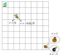
Figure 1: An example deep sea environment with $N=8$ Osband et al. [2017].

The experiment results are shown in Figure 2. From the plots, we can see that in both settings, SSR performs significantly better than RLSVI as predicted by our theory. Specifically, because of the instability incurred by the independent random seeds and large perturbation magnitude, RLSVI almost never reaches the lower right corner in both settings and thus incurs linear regret. On the other hand, SSR obtains a much lower sub-linear regret because it can explore consistently with the single random seed.

Meanwhile, in both settings, SSR performs comparably with the UCBVI, which is expected since both algorithms achieve the minimax lower bound and our analysis does not indicate that one is better than the other.

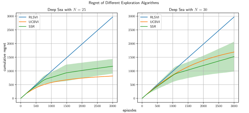
Figure 2: Empirical evaluation of RLSVI, UCBVI and SSR in deep sea environments with $N=25$ and $N=30$. The results are averaged over 10 repeated trials and the shaded area represents the standard deviation. For simplicity, we use Hoeffding-type bonus for both UCBVI and SSR.

Finally, we also do an ablation study to show that the better performance of SSR over the RLSVI indeed comes from the single seed randomization instead of smaller noise magnitude. In particular, we run both algorithms in a deep sea environment with $N=25$ and apply the same noise magnitude, whose results are shown in Figure 3. We can see that although using the same noise magnitude, SSR  still significantly outperforms RLSVI.

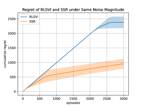
Figure 3: Empirical evaluation of RLSVI and SSR in deep sea environments with $N=25$, where both algorithms use the same noise magnitude.

References

- Abeille and Lazaric (2017) Marc Abeille and Alessandro Lazaric. Linear thompson sampling revisited. In Artificial Intelligence and Statistics, pages 176–184. PMLR, 2017.
- Agrawal et al. (2021) Priyank Agrawal, Jinglin Chen, and Nan Jiang. Improved worst-case regret bounds for randomized least-squares value iteration. Thirty-fifth AAAI conference on artificial intelligence, 2021.
- Agrawal and Goyal (2012) Shipra Agrawal and Navin Goyal. Analysis of thompson sampling for the multi-armed bandit problem. In Conference on learning theory, pages 39–1. JMLR Workshop and Conference Proceedings, 2012.
- Agrawal and Goyal (2017) Shipra Agrawal and Navin Goyal. Near-optimal regret bounds for thompson sampling. J. ACM, 64(5), September 2017. ISSN 0004-5411. doi: 10.1145/3088510. URL https://doi.org/10.1145/3088510.
- Agrawal and Jia (2017a) Shipra Agrawal and Randy Jia. Optimistic posterior sampling for reinforcement learning: worst-case regret bounds. In Advances in Neural Information Processing Systems, pages 1184–1194, 2017a.
- Agrawal and Jia (2017b) Shipra Agrawal and Randy Jia. Posterior sampling for reinforcement learning: worst-case regret bounds. In Advances in Neural Information Processing Systems, pages 1184–1194, 2017b.
- Azar et al. (2017) Mohammad Gheshlaghi Azar, Ian Osband, and Rémi Munos. Minimax regret bounds for reinforcement learning. In Proceedings of the 34th International Conference on Machine Learning-Volume 70, pages 263–272. JMLR. org, 2017.
- Bartlett and Tewari (2009) Peter L Bartlett and Ambuj Tewari. Regal: A regularization based algorithm for reinforcement learning in weakly communicating mdps. In Proceedings of the Twenty-Fifth Conference on Uncertainty in Artificial Intelligence, pages 35–42. AUAI Press, 2009.
- Brafman and Tennenholtz (2003) Ronen I. Brafman and Moshe Tennenholtz. R-max - a general polynomial time algorithm for near-optimal reinforcement learning. J. Mach. Learn. Res., 3(Oct):213–231, March 2003. ISSN 1532-4435.
- Bubeck and Liu (2014) Sébastien Bubeck and Che-Yu Liu. Prior-free and prior-dependent regret bounds for thompson sampling. In 2014 48th Annual Conference on Information Sciences and Systems (CISS), pages 1–9. IEEE, 2014.
- Burda et al. (2018) Yuri Burda, Harrison Edwards, Amos Storkey, and Oleg Klimov. Exploration by random network distillation. arXiv preprint arXiv:1810.12894, 2018.
- Cai et al. (2019) Qi Cai, Zhuoran Yang, Chi Jin, and Zhaoran Wang. Provably efficient exploration in policy optimization. arXiv preprint arXiv:1912.05830, 2019.
- Chapelle and Li (2011) Olivier Chapelle and Lihong Li. An empirical evaluation of thompson sampling. In Advances in neural information processing systems, pages 2249–2257, 2011.
- Dann and Brunskill (2015) Christoph Dann and Emma Brunskill. Sample complexity of episodic fixed-horizon reinforcement learning. In Advances in Neural Information Processing Systems, pages 2818–2826, 2015.
- Dann et al. (2017) Christoph Dann, Tor Lattimore, and Emma Brunskill. Unifying PAC and regret: Uniform PAC bounds for episodic reinforcement learning. In Proceedings of the 31st International Conference on Neural Information Processing Systems, NIPS’17, page 5717–5727, Red Hook, NY, USA, 2017. Curran Associates Inc. ISBN 9781510860964.
- Dann et al. (2019) Christoph Dann, Lihong Li, Wei Wei, and Emma Brunskill. Policy certificates: Towards accountable reinforcement learning. In Proceedings of the 36th International Conference on Machine Learning, volume 97 of Proceedings of Machine Learning Research, pages 1507–1516, Long Beach, California, USA, 09–15 Jun 2019. PMLR.
- Domingues et al. (2021) Omar Darwiche Domingues, Pierre Ménard, Emilie Kaufmann, and Michal Valko. Episodic reinforcement learning in finite mdps: Minimax lower bounds revisited. In Algorithmic Learning Theory, pages 578–598. PMLR, 2021.
- Dong et al. (2019) Kefan Dong, Yuanhao Wang, Xiaoyu Chen, and Liwei Wang. Q-learning with ucb exploration is sample efficient for infinite-horizon mdp. arXiv preprint arXiv:1901.09311, 2019.
- Fortunato et al. (2018) Meire Fortunato, Mohammad Gheshlaghi Azar, Bilal Piot, Jacob Menick, Matteo Hessel, Ian Osband, Alex Graves, Volodymyr Mnih, Remi Munos, Demis Hassabis, et al. Noisy networks for exploration. In International Conference on Learning Representations, 2018.
- Fruit et al. (2018) Ronan Fruit, Matteo Pirotta, and Alessandro Lazaric. Near optimal exploration-exploitation in non-communicating markov decision processes. In Advances in Neural Information Processing Systems, pages 2994–3004, 2018.
- Jaksch et al. (2010) Thomas Jaksch, Ronald Ortner, and Peter Auer. Near-optimal regret bounds for reinforcement learning. Journal of Machine Learning Research, 11(Apr):1563–1600, 2010.
- Jin et al. (2018) Chi Jin, Zeyuan Allen-Zhu, Sebastien Bubeck, and Michael I Jordan. Is Q-learning provably efficient? In Advances in Neural Information Processing Systems, pages 4863–4873, 2018.
- Jin et al. (2019) Chi Jin, Zhuoran Yang, Zhaoran Wang, and Michael I Jordan. Provably efficient reinforcement learning with linear function approximation. arXiv preprint arXiv:1907.05388, 2019.
- Jin et al. (2020) Tianyuan Jin, Pan Xu, Jieming Shi, Xiaokui Xiao, and Quanquan Gu. Mots: Minimax optimal thompson sampling. arXiv preprint arXiv:2003.01803, 2020.
- Kakade (2003) Sham M Kakade. On the sample complexity of reinforcement learning. PhD thesis, University of London London, England, 2003.
- Kaufmann et al. (2012) Emilie Kaufmann, Nathaniel Korda, and Rémi Munos. Thompson sampling: An asymptotically optimal finite-time analysis. In International conference on algorithmic learning theory, pages 199–213. Springer, 2012.
- Kearns and Singh (2002) Michael Kearns and Satinder Singh. Near-optimal reinforcement learning in polynomial time. Machine learning, 49(2-3):209–232, 2002.
- Kolter and Ng (2009) J Zico Kolter and Andrew Y Ng. Near-bayesian exploration in polynomial time. In Proceedings of the 26th annual international conference on machine learning, pages 513–520, 2009.
- Lai and Robbins (1985) Tze Leung Lai and Herbert Robbins. Asymptotically efficient adaptive allocation rules. Advances in applied mathematics, 6(1):4–22, 1985.
- Lattimore and Hutter (2012) Tor Lattimore and Marcus Hutter. Pac bounds for discounted mdps. In International Conference on Algorithmic Learning Theory, pages 320–334. Springer, 2012.
- Li et al. (2021) Gen Li, Laixi Shi, Yuxin Chen, Yuantao Gu, and Yuejie Chi. Breaking the sample complexity barrier to regret-optimal model-free reinforcement learning. Advances in Neural Information Processing Systems, 34, 2021.
- Maurer and Pontil (2009) Andreas Maurer and Massimiliano Pontil. Empirical Bernstein bounds and sample variance penalization. arXiv preprint arXiv:0907.3740, 2009.
- Menard et al. (2021) Pierre Menard, Omar Darwiche Domingues, Xuedong Shang, and Michal Valko. Ucb momentum q-learning: Correcting the bias without forgetting. arXiv preprint arXiv:2103.01312, 2021.
- Neu and Pike-Burke (2020) Gergely Neu and Ciara Pike-Burke. A unifying view of optimism in episodic reinforcement learning. arXiv preprint arXiv:2007.01891, 2020.
- Osband and Van Roy (2017) Ian Osband and Benjamin Van Roy. Why is posterior sampling better than optimism for reinforcement learning? In Proceedings of the 34th International Conference on Machine Learning-Volume 70, pages 2701–2710. JMLR. org, 2017.
- Osband et al. (2013) Ian Osband, Daniel Russo, and Benjamin Van Roy. (more) efficient reinforcement learning via posterior sampling. In Advances in Neural Information Processing Systems, pages 3003–3011, 2013.
- Osband et al. (2014) Ian Osband, Benjamin Van Roy, and Zheng Wen. Generalization and exploration via randomized value functions. arXiv preprint arXiv:1402.0635, 2014.
- Osband et al. (2017) Ian Osband, Daniel Russo, Zheng Wen, and Benjamin Van Roy. Deep exploration via randomized value functions. arXiv preprint arXiv:1703.07608, 2017.
- Osband et al. (2018) Ian Osband, John Aslanides, and Albin Cassirer. Randomized prior functions for deep reinforcement learning. In Advances in Neural Information Processing Systems, pages 8617–8629, 2018.
- Pacchiano et al. (2020) Aldo Pacchiano, Philip Ball, Jack Parker-Holder, Krzysztof Choromanski, and Stephen Roberts. On optimism in model-based reinforcement learning. arXiv preprint arXiv:2006.11911, 2020.
- Russo (2019) Daniel Russo. Worst-case regret bounds for exploration via randomized value functions. In Advances in Neural Information Processing Systems, pages 14433–14443, 2019.
- Simchowitz and Jamieson (2019) Max Simchowitz and Kevin G Jamieson. Non-asymptotic gap-dependent regret bounds for tabular mdps. In Advances in Neural Information Processing Systems, pages 1153–1162, 2019.
- Strehl and Littman (2008) Alexander L Strehl and Michael L Littman. An analysis of model-based interval estimation for markov decision processes. Journal of Computer and System Sciences, 74(8):1309–1331, 2008.
- Strehl et al. (2006) Alexander L Strehl, Lihong Li, Eric Wiewiora, John Langford, and Michael L Littman. Pac model-free reinforcement learning. In Proceedings of the 23rd international conference on Machine learning, pages 881–888. ACM, 2006.
- Szita and Szepesvári (2010) István Szita and Csaba Szepesvári. Model-based reinforcement learning with nearly tight exploration complexity bounds. In ICML, 2010.
- Talebi and Maillard (2018) Mohammad Sadegh Talebi and Odalric-Ambrym Maillard. Variance-aware regret bounds for undiscounted reinforcement learning in mdps. arXiv preprint arXiv:1803.01626, 2018.
- Tan et al. (2020) Tian Tan, Zhihan Xiong, and Vikranth R Dwaracherla. Parameterized indexed value function for efficient exploration in reinforcement learning. In Proceedings of the AAAI Conference on Artificial Intelligence, volume 34, pages 5948–5955, 2020.
- Vaswani et al. (2020) Sharan Vaswani, Abbas Mehrabian, Audrey Durand, and Branislav Kveton. Old dog learns new tricks: Randomized ucb for bandit problems. In Proceedings of the Twenty Third International Conference on Artificial Intelligence and Statistics, pages 1988–1998, 2020.
- Wang et al. (2020) Ruosong Wang, Simon S Du, Lin F Yang, and Sham M Kakade. Is long horizon reinforcement learning more difficult than short horizon reinforcement learning? arXiv preprint arXiv:2005.00527, 2020.
- Xu and Tewari (2019) Ziping Xu and Ambuj Tewari. Worst-case regret bound for perturbation based exploration in reinforcement learning. Ann Arbor, 1001:48109, 2019.
- Yang et al. (2020) Kunhe Yang, Lin F Yang, and Simon S Du. -learning with logarithmic regret. arXiv preprint arXiv:2006.09118, 2020.
- Zanette and Brunskill (2019) Andrea Zanette and Emma Brunskill. Tighter problem-dependent regret bounds in reinforcement learning without domain knowledge using value function bounds. In International Conference on Machine Learning, pages 7304–7312, 2019.
- Zanette et al. (2020) Andrea Zanette, David Brandfonbrener, Emma Brunskill, Matteo Pirotta, and Alessandro Lazaric. Frequentist regret bounds for randomized least-squares value iteration. In International Conference on Artificial Intelligence and Statistics, pages 1954–1964, 2020.
- Zhang and Ji (2019) Zihan Zhang and Xiangyang Ji. Regret minimization for reinforcement learning by evaluating the optimal bias function. In Advances in Neural Information Processing Systems, pages 2823–2832, 2019.
- Zhang et al. (2020a) Zihan Zhang, Xiangyang Ji, and Simon S Du. Is reinforcement learning more difficult than bandits? a near-optimal algorithm escaping the curse of horizon. arXiv preprint arXiv:2009.13503, 2020a.
- Zhang et al. (2020b) Zihan Zhang, Yuan Zhou, and Xiangyang Ji. Almost optimal model-free reinforcement learning via reference-advantage decomposition. arXiv preprint arXiv:2004.10019, 2020b.
- Zhang et al. (2020c) Zihan Zhang, Yuan Zhou, and Xiangyang Ji. Model-free reinforcement learning: from clipped pseudo-regret to sample complexity. arXiv preprint arXiv:2006.03864, 2020c.