Ge, Wang, Xiong, Ye

From an Interior Point to a Corner Point: Smart Crossover

From an Interior Point to a Corner Point: Smart Crossover

Dongdong Ge Research Institute for Interdisciplinary Sciences, Shanghai University of Finance and Economics, Shanghai, 200433, China. ge.dongdong@shufe.edu.cn Chengwenjian Wang Department of Industrial and Systems Engineering, Univesity of Minnesota, Minneapolis, MN, 55414, USA. wcwj@umn.edu Zikai Xiong MIT Operations Research Center, Cambridge, MA, 02139, USA. zikai@mit.edu Yinyu Ye Department of Management Science and Engineering, Stanford University, Stanford, CA, 94305, USA. yyye@stanford.edu

Identifying optimal basic feasible solutions to linear programming problems is critical for mixed integer programming and other applications. The crossover method, which aims at deriving an optimal extreme point from a suboptimal solution (the output of a starting method such as interior-point methods or first-order methods), is crucial in this process. This method, compared with the starting method, frequently represents the primary computational bottleneck in practical applications. We propose some approaches to overcome this bottleneck by smartly exploiting problem characteristics and implementing customized strategies. For problems arising from network applications and exhibiting network structures, we take advantage of the graph structure of the problem and the tree structure of the optimal solutions. Based on these structures, we propose a tree-based crossover method, aimed at recovering basic solutions by identifying nearby spanning tree structures. For general linear programs, we propose to recover an optimal basic solution by identifying the optimal face and employing controlled perturbations based on the suboptimal solution provided by interior-point methods. We prove that an optimal solution for the perturbed problem is an extreme point, and its objective value is at least as good as that of the initial interior point solution. Computational experiments show significant speed-ups achieved by our methods compared to state-of-the-art commercial solvers on classical linear programming problem benchmarks, network flow problem benchmarks, and optimal transport problems.

linear programming; optimal transport; network flow problem; first-order method; interior-point method

1 Introduction

Linear Program (LP) is a fundamental problem and important tool in operations research, widely used in various applications like transportation, scheduling, inventory control, and revenue management (Bowman 1956, Charnes and Cooper 1954, Hanssmann and Hess 1960, Liu and Van Ryzin 2008). In LP problems, basic feasible solutions (BFS) – also known as corner points – correspond identically to vertices and extreme points of the feasible set. These solutions are particularly important for several reasons: Firstly, to warm start the simplex method, a BFS is required. Secondly, a BFS, compared to other feasible points, has an inclusive-maximal set of active constraints. This feature is especially valuable for certain applications, such as discrete optimization problems. Additionally, in integer programming, finding the optimal BFS for LP relaxation problems is essential. In certain instances, such as network flow problems with integral right-hand side vectors, an optimal BFS is inherently integral. In such cases, finding an optimal BFS for the LP relaxation is all that is needed to address the integer program.

1.1 Challenges for Current Crossover Approaches

Crossover allows us to combine the advantages of both simplex algorithms and interior-point methods, the two classic algorithms that have driven advancements in operations research for decades. Simplex algorithms perform pivot iterations through basic solutions, ultimately yielding an optimal BFS. Simplex algorithms are usually very powerful in practice, but can be inefficient for some problems. In contrast, interior-point methods might converge faster in both theory and practice for these problems, but they return an interior-point solution rather than a BFS. By employing the crossover approach, it is possible to leverage the speed of interior-point methods for such problems while still obtaining a BFS.

Crossover in LP solvers.

Crossover has been an essential research topic in conjunction with the studies on interior-point methods. Megiddo (1991) demonstrated that, given a complementary primal-dual pair of solutions, an optimal BFS could be identified after at most $n$ pivots, where $n$ denotes the number of variables. In each pivot, one variable is pushed to the upper or lower bound while the solution remains optimal and feasible. Although the theory is elegant, crossover in practice might not fulfill the guarantees of the theoretical results, as it begins with a solution that is only approximately complementary and feasible. To address this issue, Bixby and Saltzman (1994) proposed an approach that first identified a near-optimal candidate basis, which might even be infeasible, by ranking the magnitude of variables’ distances to the bounds. They then adapted Wolfe’s piecewise-linear phase I algorithm (Wolfe 1965). Upon reaching a primal feasible solution, they applied Cplex’s phase-II algorithm to solve for the optimal solution. Indeed, Megiddo’s crossover is a special case of Bixby and Saltzman’s method, which was then included in Cplex 2.2 (Bixby 1994). Furthermore, Andersen and Ye (1996) showed that once the interior-point method’s solution was sufficiently accurate, it formed an optimal complementary primal-dual pair for a modified LP, whose optimal basis was an optimal basis for the original problem. In this case, directly adopting Megiddo’s approach for the modified problem yields an optimal basis for the original problem. However, Andersen (1999) noted that ensuring the accuracy of the interior-point method remained challenging, and the basis obtained could still be infeasible; thus, more pivots are necessary to start from the obtained candidate basis in practice. This approach was subsequently implemented by MOSEK (Andersen and Andersen 2000).

In general, the procedure of solving an LP typically contains the following three phases, in which we call the second and third phases the crossover.

• Starting method: Obtain a suboptimal solution via a “starting method”, which is usually an interior-point method in commercial solvers.

• Basis Identification: Identify a candidate basis from the suboptimal solution and then perform pivots to obtain a nearby primal/dual feasible basis.

• Reoptimization: Adopt primal/dual simplex algorithms starting from the obtained primal/dual feasible basis until reaching an optimal BFS.

The commercial solver Gurobi adopts a similar strategy but it names the task of identifying a candidate basis “push” and the task of performing pivots “cleanup” (Maes et al. 2014, Gurobi Optimization, LLC 2023). Since the distance of the candidate basis to feasible or optimal bases is unknown, crossover’s running time lacks a reliable theoretical estimate.

In spite of crossover’s significance for practical performance and competitiveness in the solver industry, the literature on this topic is not as extensive as one might expect. Berkelaar et al. (1999) extended crossover to quadratic programming. Glavelis et al. (2018) applied the idea of crossover to accelerate the exterior-point simplex algorithms. Schork and Gondzio (2020) proposed an interior-point method with basis preconditioning and its associated crossover approach. Galabova and Hall (2020) revealed that the open-source solver Clp (CORE-OR 2023) implements a crash method (whose the idea comes from Forrest and Goldfarb (1992)) to increase the sparsity of the given solution via a penalty method. El-Bakry et al. (1994) and Ye (1992) studied how to identify the optimal face (or the active constraints at optima); in the special case of non-degeneracy, it is equivalent to identifying the optimal BFS.

Challenges for modern crossover.

In many recent real LP applications, the crossover has become a crucial component, on average taking over a quarter of the overall running time, as Maes et al. (2014) presented. Given the lack of guarantees on the quality of the candidate basis, the number of pivots could frequently be enormous, especially for huge-scale problems. On the other hand, these large-scale instances are becoming increasingly common in real-world applications.

The challenges for crossover also stem from the specificities of new methods used as the starting method. For general-purpose LP problems, many first-order methods have been proposed recently to address the huge-scale applications (O’donoghue et al. 2016, Lin et al. 2020, Deng et al. 2022, Applegate et al. 2021, Li et al. 2020, Lu and Yang 2023, Wang et al. 2023). Although first-order methods can handle larger-scale LPs, there is a recognized challenge in obtaining a reliable and highly accurate solution. The challenge emphasizes the need for further improvements of crossover methods. Furthermore, for LPs with special structures, fast problem-focused first-order algorithms have been proposed (Cuturi 2013, Ge et al. 2019, Altschuler et al. 2017, Gao et al. 2021). These methods usually do not obtain basic solutions, and the traditional crossover method, designed for general-purpose LPs, cannot utilize the special structure of the problem either. This limitation makes the crossover a computational bottleneck in solving such structured LP problems.

Furthermore, in some cases, obtaining a nearly-optimal BFS within a given tolerance is sufficient. Compared with the usual aim of finding an optimal BFS, potential running time benefits could have come from early stopping the starting method and dropping the phase of reoptimization. However, the running time of the basis identification phase and the optimality error of the BFS obtained rely on the quality of the solution returned by the starting method, which means early stopping the starting method cannot guarantee benefits and sometimes even hurt. To deal with this issue, Mehrotra (1991) proposed a controlled perturbation strategy on the objective vector so that the perturbed problem only has a unique optimal solution. When the optimal solution is unique, the optimal basis could be identified more easily (Tapia and Zhang 1991). While Mehrotra’s perturbation strategy has demonstrated promising results in practical tests, the obtained BFS cannot be guaranteed with a better objective than the given solution from the starting method.

In this paper, we propose two novel crossover approaches to address those issues. First, for the minimum cost flow (MCF) problem and other problems with a network structure, we present a crossover approach that exploits the graph structure of the problem and the tree structure of the BFS. This approach allows us to efficiently identify an optimal or near-optimal basis, even if we start from a low-accuracy solution from the starting method. Second, for general LP problems, we propose an alternative crossover approach based on optimal face detection and a minor perturbation. This approach aims to obtain a near-optimal BFS whose objective is at least as good as the solution given by an interior-point method.

1.2 Minimum Cost Flow Problem

As a prominent and important case of LP, the minimum cost flow (MCF) problem possesses a notable property: its incidence matrix is totally unimodular. This means that when the right-hand side vector (in the standard form) is integral, every basic solution is also integer-valued. In this case, if the problem is the LP relaxation of an integer program, one gets an integer solution for free by solving the LP to an optimal BFS. It is worth mentioning that the per-iteration complexity of the simplex method can be significantly reduced using the network simplex method (Ahuja et al. 1993), although it sometimes still suffers from the scale of the problem and may require special pivoting rules. Fast algorithms have been proposed to deal with some special cases, such as (Applegate et al. 2021) for huge-scale problems, and the Sinkhorn method (Cuturi 2013) for optimal transport problems. These new methods are usually not designed to obtain the optimal solution that is BFS so a followed crossover is required for getting an optimal BFS.

The optimal transport problem, as a class of MCF problems, is an important research topic with applications in mathematics (Santambrogio 2015), economics (Galichon 2018), and machine learning (Nguyen 2013, Ho et al. 2019). Machine learning applications in particular place huge demands on the calculation efficiency of optimal transport problems. Due to the usage of entropy regularization, the Sinkhorn algorithm (Cuturi 2013) has significantly reduced this complexity and triggered a series of research works on different regularization terms. However, due to the regularization terms, in spite of the increased speed, the solution obtained by these methods is not an optimal BFS.

1.3 Our Contributions

In this paper, for simplicity of notation, we consider problems in the following standard form:

$$\min_{x\in\mathbb{R}^{n}}\,\,\,\,c^{\top}x\quad\operatorname{s.t.}\,\,Ax=b,~{}x\geq 0,$$ (1)

where $A\in\mathbb{R}^{m\times n}$, $c\in\mathbb{R}^{n}$ and $b\in\mathbb{R}^{m}$.

• For LP problems with an inherent network structure, we propose two basis identification strategies and the corresponding crossover approaches. Based on the spanning tree characteristics of BFS, we develop a tree-based basis identification method. For problems with a large number of arcs, we develop a column-based strategy. These basis identification phases do not require any knowledge of the dual solution but exploit the graph structure of the problem. Experiments with MCF problems are conducted on public network flow datasets, and optimal transport problems are tested on the MNIST dataset. Compared with commercial solvers’ crossover, our crossover method exhibits significant speed-ups, especially when the given starting method solution is only of low accuracy. Furthermore, we also describe how the combination of first-order methods, such as the Sinkhorn algorithm, and our crossover method, has advantages in practice.

• For general LP problems, we propose a crossover approach that first identifies an approximate optimal face via the primal-dual solution pair and then finds a high-quality near-optimal BFS via adopting a minor perturbation. Depending on the requirements of applications, the reoptimization phase can be carried out via the primal or dual simplex method. Experiments on LP benchmark problems reveal that our crossover method can notably enhance the performance of state-of-the-art commercial solvers, particularly on currently challenging problems.

1.4 Outline

In Section 2, we introduce some preliminaries and background. In Section 3, we propose a network structure based crossover method for MCF problems and its extension to general LP problems. In Section 4, we propose a perturbation crossover method to accelerate the crossover procedure in general-purpose LP solvers. The computational results are presented in Section 5.

1.5 Notation

We use $[n]$ to denote the set $\{1,2,\dots,n\}$. For a set $\mathcal{X}$, the notation $|\mathcal{X}|$ denotes the cardinality of $\mathcal{X}$. For $\mathcal{X}\subseteq[n]$ and vector $u\in\mathbb{R}^{n}$, $u_{\mathcal{X}}$ is the $|\mathcal{X}|$-vector constituted by the components of $u$ with indices in $\mathcal{X}$. For a matrix $X$ and scalar $x$, $X\geq x$ means each component of $X$ is greater than or equal to $x$. For a matrix $A=(A)_{ij}$, the positive part and negative part of $A$ are $A^{+}$ and $A^{-}$, $(A^{+})_{ij}:=\max\{(A)_{ij},~{}0\},$ and $(A^{-})_{ij}:=\max\{-(A)_{ij},0\}.$ $A_{i\cdot}$, $A_{\cdot j}$ and $A_{ij}$ denote the $i$-th row, $j$-th column and the component in the $i$-th row and the $j$-th column of $A$, respectively. For a graph $(\mathcal{N},\mathcal{A})$ and $i\in\mathcal{N}$, $\mathcal{O}(i),\mathcal{I}(i)$ denote the node sets connecting to i, specifically, $\mathcal{O}(i):=\{j:(i,j)\in\mathcal{A}\},\mathcal{I}(i):=\{j:(j,i)\in\mathcal{A}\}$. And for any two sets $\mathcal{X}$ and $\mathcal{Y}$, we use $\mathcal{X}\setminus\mathcal{Y}$ to denote $\{x:x\in\mathcal{X}\text{ but }x\notin\mathcal{Y}\}$. We denote the Euclidean norm using $\|\cdot\|$. For any set $\mathcal{X}$, we use $P_{\mathcal{X}}(\cdot)$ to denote the projection onto $\mathcal{X}$, i.e., $P_{\mathcal{X}}(z):=\arg\min_{\hat{z}\in\mathcal{X}}\|z-\hat{z}\|$. For a matrix $A\in\mathbb{R}^{n\times n}$, we use $A^{\dagger}$ to denote the Moore–Penrose inverse of $A$. Moreover, we use $\operatorname{Null}(A)$ and $\operatorname{Im}(A)$ to denote the null space and image space of the matrix $A$, respectively, when viewed as a linear map.

2 Preliminaries

MCF problem.

Let $\mathcal{G}=(\mathcal{N},\mathcal{A})$ be a directed graph consisting of nodes $\mathcal{N}$ and arcs $\mathcal{A}$. Each node $i\in\mathcal{N}$ is associated with a signed supply value $b_{i}$. Each arc $(i,j)\in\mathcal{A}$ is associated with a capacity $u_{ij}$ (possibly infinite) and a cost $c_{ij}$ per unit of flow. Then the MCF problem is defined as

$$\begin{array}[]{ll}\min_{f}&\sum_{(i,j)\in\mathcal{A}}c_{ij}f_{ij}\\ \operatorname{s.t.}&b_{i}+\sum_{j\in\mathcal{I}(i)}f_{ji}=\sum_{j\in\mathcal{O}(i)}f_{ij},~{}\forall~{}i\in\mathcal{N},\text{ and }0\leq f_{ij}\leq u_{ij},\ \forall\ (i,j)\in\mathcal{A},\end{array}$$ (2)

where $\mathcal{O}(i):=\{j:(i,j)\in\mathcal{A}\}$, $\mathcal{I}(i):=\{j:(j,i)\in\mathcal{A}\}$.

Optimal transport problem.

The optimal transport problem is a special equivalent form of the general MCF problems. Following the definition of the general MCF problem, the nodes $\mathcal{N}$ can be divided into two groups, suppliers $\mathcal{S}$ and consumers $\mathcal{C}$. And arcs $\mathcal{A}$ pairwisely connect suppliers and consumers, in the direction from the former to the latter, i.e., $\mathcal{A}=\mathcal{S}\times\mathcal{C}:=\{(i,j):i\in\mathcal{S},j\in\mathcal{C}\}$. For any supplier $i$ and consumer $j$, $s_{i}$ and $d_{j}$ respectively denote the capacity of the supply and demand. Then an optimal transport problem can be rewritten as follows:

$$\begin{array}[]{lll}\operatornamewithlimits{min}_{f}&\sum_{(i,j)\in\mathcal{S}\times\mathcal{C}}c_{ij}f_{ij}\\ \operatorname{s.t.}&\sum_{j\in\mathcal{C}}f_{ij}=s_{i},~{}\forall~{}i\in\mathcal{S},\ \sum_{i\in\mathcal{S}}f_{ij}=d_{j},~{}\forall j\in\mathcal{C},\text{ and }f_{ij}\geq 0,~{}\forall~{}(i,j)\in\mathcal{S}\times\mathcal{C}\end{array}$$ (3)

Optimal Face.

For the general primal problem (1), the dual problem is

$$\begin{array}[]{l}\operatornamewithlimits{max}_{y\in\mathbb{R}^{m},s\in\mathbb{R}^{n}}~{}b^{\top}y\quad\operatorname{s.t.}~{}A^{\top}y+s=c,~{}~{}s\geq 0\end{array}$$ (4)

Note that in textbooks such as Bertsimas and Tsitsiklis (1997), the dual problem only has decision variable $y$, but here we use the equivalent form (4) with slackness $s$ as part of variables. To be specific, for any feasible $(y,s)$, $s=c-A^{\top}y$, and for any feasible $s$, a feasible $(y,s)$ pair can be recovered by $y=(AA^{\top})^{\dagger}A(c-s)$, so we will then mainly work on $s$ instead of $y$. For (1) and (4), there exists at least one optimal solution pair $(x^{\star},s^{\star})$ that is strictly complementary (Goldman and Tucker 1956), i.e., $\mathcal{P}(x^{\star})\cap\mathcal{P}(s^{\star})=\emptyset$ and $\mathcal{P}(x^{\star})\cup\mathcal{P}(s^{\star})=[n]$, in which $\mathcal{P}(z):=\{i:z_{i}>0\}$ denotes the set of indices for the strictly positive components of $z$. Moreover, if we denote $\mathcal{P}^{\star}$ as $\mathcal{P}(x^{\star})$, and denote $\mathcal{D}^{\star}$ as $\mathcal{P}(s^{\star})$, then $\{\mathcal{P}^{\star},~{}\mathcal{D}^{\star}\}$ is called the optimal partition. Then for any optimal solutions $x^{\star}$ and $s^{\star}$, $\mathcal{P}(x)\subseteq\mathcal{P}^{\star},$ and $\mathcal{P}(s)\subseteq\mathcal{D}^{\star}$. With the above definitions, the optimal face of the primal problem (1) and dual problem (4) can be rewritten as

$$\begin{array}[]{ll}&\Theta_{p}:=\{x:Ax=b,~{}x_{\mathcal{P}^{\star}}\geq 0,\text{and }x_{\mathcal{D}^{\star}}=0\},\\ &\Theta_{d}:=\{(y,s):A^{\top}y+s=c,~{}s_{\mathcal{D}^{\star}}\geq 0,\text{ and }s_{\mathcal{P}^{\star}}=0\}.\end{array}$$ (5)

Column generation method.

The column generation method is an approach for large-scale LP problems. Instead of directly solving the original problem (1), the column generation method involves a sequence of master iterations. In each iteration, a collection of columns $A_{\cdot i}$, $i\in\Lambda$, is formed and the following restricted problem is solved:

$$LP(\Lambda):\quad\min_{x\in\mathbb{R}^{n}}~{}\sum_{i\in\Lambda}c_{i}x_{i}~{}~{}\operatorname{s.t.}~{}\sum_{i\in\Lambda}A_{\cdot i}x_{i}=b,~{}x_{[n]\setminus\Lambda}=0,~{}x_{\Lambda}\geq 0.$$ (6)

Refer to Algorithm 1 for the general framework. See Bertsimas and Tsitsiklis (1997) for specific rules of updating $\Lambda_{k}$. The collection $\Lambda_{k+1}$ contains the basis of the solution $x^{k}$ from $LP(\Lambda_{k})$, so a simple method for $LP(\Lambda_{k+1})$ can easily warm start from $x^{k}$.

Algorithm 1 General Column Generation Method

1:  Iteration counter $k=1$, and initial set of columns $\Lambda_{1}$.

2:  while the reduced cost $\bar{c}\ngeq 0$ do

3:     Update column set: Update $\Lambda_{k}$ according to some rules.

4:     Solve the restricted problem: Solve $LP(\Lambda_{k})$ and obtain an optimal basis $B_{k}$.

5:     Compute reduced cost: $\bar{c}\leftarrow c-c^{\top}_{B_{k}}B_{k}^{-1}A$, and $k\leftarrow k+1$.

6:  end while

3 Network Crossover Method

As already mentioned in Section 1, traditional crossover methods select the candidate basis by directly ranking the magnitude of variables or comparing ratios between variables. However, these methods do not take the graph structure of the problem into account.

We first use an optimal transport example to show that ranking the magnitude of variables may introduce errors. Figure 1 illustrates an example of a small optimal transport problem with supply nodes in blue and demand nodes in brown. The supplies, demands, and transportation costs per unit are displayed in Figure 1a. Suppose that we are given a central-path solution generated by a starting method such as a typical path-following interior-point method, and this solution has an objective value that is 7% higher than the optimal objective value. Then the relative variable values of this solution are represented in the arc widths of Figure 1b. The arc in green denotes the variables in the optimal basis and the arc in red denote the variables not in the optimal basis. From the problem setting, the arc $(S3,D3)$ should be included in the optimal basis; however, its width is not as great as that of arcs $(S2,D1)$ or $(S2,D3)$. Indeed, by taking into account the graph structure, since every basis corresponds to a spanning tree, the optimal basis must contain an arc that originates from node $S3$. Therefore, in this section, we will define flow ratio (whose relative value is represented the arc widths in Figure 1c) to depict the graph structure and do the crossover.

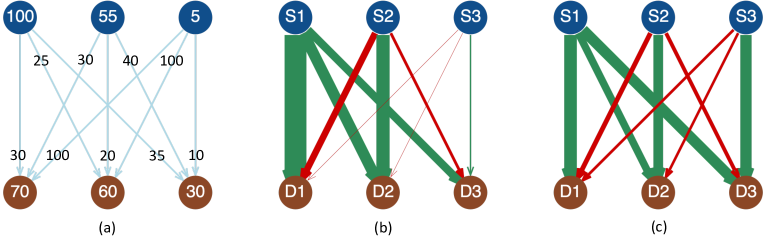
Figure 1: An example of an optimal transport problem, with supply nodes in blue and demand nodes in brown. Figure (a) presents the problem coefficients of supplies, demands, and transportation costs per unit. Figure (b) shows the relative values of an interior solution as the line width of arcs. Figure (c) shows the relative flow ratios defined in (7) as the line width of arcs.

Before we define the flow ratio, we first transform the MCF problem into an uncapacitated problem based on variables of the given suboptimal solution. Assume that we have obtained a feasible suboptimal solution $\tilde{f}$ for the problem (2), denoted as $MCF(b,c,u)$, through a starting method. In this case, there exists a transformation of the problem variables such that each $\tilde{f}_{ij}$ is closer to the lower bound $0$ than the capacity upper bound $u_{ij}$. Specifically, let $\mathcal{L}:=\{(i,j)\in\mathcal{A}:\tilde{f}_{ij}-0<u_{ij}-\tilde{f}_{ij}\}$ and $\mathcal{U}:=\mathcal{A}\setminus\mathcal{L}$. Our requirement is then satisfied by replacing variables $f_{\mathcal{U}}$ in $MCF(b,c,u)$ with $u_{\mathcal{U}}-f_{\mathcal{U}}$. We denote the problem after the variable transformation as $MCF(\bar{b},\bar{c},\bar{u})$. Note that if $\tilde{f}$ is already an optimal solution of $MCF(b,c,u)$, then the corresponding $MCF(\bar{b},\bar{c},\bar{u})$ has an optimal solution that is never active in any constraint of the capacity upper bound. Moreover, when $\tilde{f}$ is close enough to the optimal solutions (for example, when the $l_{\infty}$ norm distance is smaller than $\frac{1}{2}\min_{i}|\bar{u}_{i}|$), $MCF(\bar{b},\bar{c},\bar{u})$ shares the same optimal solutions with the uncapacitated MCF problem $MCF(\bar{b},\bar{c},\infty)$. Also, any optimal BFS of $MCF(\bar{b},\bar{c},\infty)$, after being transformed back to the original MCF problem, remains an optimal BFS of the original problem. Consequently, to identify a near-optimal basis for $MCF(b,c,u)$, we can instead identify a near-optimal basis for $MCF(\bar{b},\bar{c},\infty)$ by constructing a nearby basis for the transformation of the given flow vector $\tilde{f}$.

In uncapacitated MCF problems, a solution $f$ is a basic (feasible) solution if and only if it is a (feasible) tree solution (Ahuja et al. 1993). The tree solutions in uncapacitated MCF problems are those whose nonzero components can form a spanning tree without considering the direction of flows. For a nondegenerate BFS of the uncapacitated MCF problem in a connected graph, there are exactly $|\mathcal{N}|-1$ strictly positive flows (positive components of the BFS), connecting each node in the graph and corresponding to a spanning tree in $\mathcal{G}$. Taking into account the tree structure of basic solutions, we will select $|\mathcal{N}|-1$ arcs in a specific order. For a nonbasic suboptimal feasible solution, the arc that delivers the most flow to a single node has a higher likelihood and priority to be in the basis compared to other flows. Therefore, we use the following flow ratio to measure the potential of an arc to be part of an optimal basis.

Given any flow $f$ of a directed graph $\mathcal{G}=(\mathcal{N},\mathcal{A})$, for each arc $(i,j)$ in $\mathcal{A}$, the flow ratio is defined as the maximum proportion of the flow that $f_{ij}$ serves over the total flow that passes node $i$ or $j$, i.e.,

$$r_{ij}:=\max\left\{\frac{f_{ij}}{\sum_{l\in\mathcal{O}(i)}f_{il}+\sum_{l\in\mathcal{I}(i)}f_{li}},\ \frac{f_{ij}}{\sum_{l\in\mathcal{O}(j)}f_{jl}+\sum_{l\in\mathcal{I}(j)}f_{lj}}\right\}\ .$$ (7)

The flow ratio measures the proportion that the flow in a specific arc serves in all the conjoint arcs. All optimal solutions are convex combinations of optimal basic feasible solutions, so for any method generating iterates that converge to optimal solutions, the flow ratio of the arcs that are never in any optimal basis would converge to zero. Unlike traditional indicators that only consider the magnitude of the arc, the flow ratio takes into account the connected nodes and all adjacent arcs. For instance, in Figure 1c, the linewidths represent the relative flow ratios, which align better with the optimal basis than when solely using variable values in Figure 1b. Although no strong theoretical guarantee exists for these indicators just like the indicators in traditional crossover methods, based on them we will provide two crossover methods that are powerful in practice.

Recall that after the starting method, the crossover phase is composed of two phases, namely basis identification and reoptimization. Let arcs be ranked in descending order based on their corresponding flow ratios and form the array $(s_{1},s_{2},\dots,s_{|\mathcal{A}|})$ of $\mathcal{A}$. Then based on this order, we propose two crossover methods for the basis identification phase.

3.1 Tree-based Basis Identification (Tree-BI)

Similarly to the standard crossover, the basis identification first identifies a candidate basis and then obtains a nearby feasible basis as a starting point for reoptimization. Since the BFS of any MCF problem has to be a feasible tree solution, and a tree solution corresponds to a spanning tree in the graph, candidate bases can be identified from the construction of a spanning tree. If the given suboptimal solution is of sufficient accuracy and the optimal solution is unique, such a spanning tree corresponds exactly to the optimal BFS. This spanning tree problem can be efficiently solved using combinatorial algorithms for minimum spanning tree problems (Prim 1957, Dijkstra et al. 1959, Chazelle 2000). When the suboptimal solution is not of sufficient accuracy, the obtained basis may still be infeasible. In such cases, in a fashion similar to traditional crossover methods, a piecewise-linear phase I simplex method is then required to find a nearby feasible basis.

For the special case of optimal transport problems, the following proposition enables us to design an efficient phase I method for obtaining a feasible basis:

Proposition 3.1

For the optimal transport problem (3), suppose that the basic solution/flow $f$ is infeasible, say $f_{ij}<0$, for $(i,j)\in\mathcal{A}$. Then, there exist $j^{\prime},i^{\prime}\in\mathcal{N}$ such that $(i,j^{\prime})$, $(i^{\prime},j)$ are also arcs in $\mathcal{A}$ and $f_{ij^{\prime}}>0$, $f_{i^{\prime}j}>0$. Moreover, for any such $i^{\prime},j^{\prime}$, $(i^{\prime},j^{\prime})$ is also an arc in $\mathcal{A}$ and $f_{i^{\prime}j^{\prime}}=0$.

Proof 3.2

Proof. Since $(i,j)\in\mathcal{A}$, we have $i\in\mathcal{S}$ and $j\in\mathcal{C}$. Moreover, $\sum_{l\in\mathcal{C}}f_{il}=s_{i}\geq 0$ and $\sum_{l\in S}f_{lj}=d_{j}\geq 0$ due to the definition of optimal transport problems. Noting that $f_{ij}<0$, there must exist $f_{ij^{\prime}}>0$, $j^{\prime}\in\mathcal{C}$ and $f_{i^{\prime}j}>0$, $i^{\prime}\in\mathcal{S}$. Furthermore, because $i^{\prime}\in\mathcal{S}$, $j^{\prime}\in\mathcal{C}$ and $\mathcal{A}=\mathcal{S}\times\mathcal{C}$, then $(i^{\prime},j^{\prime})$ is an arc in $\mathcal{A}$. Since the subgraph corresponding to the nonzeros in $f$ is a tree, it must contain no cycle. In particular, there must be zero flow in $f_{ij},f_{ij^{\prime}},f_{i^{\prime}j},f_{i^{\prime}j^{\prime}}$, and thus $f_{i^{\prime}j^{\prime}}=0$.

Using this result, we can eliminate the negative flows of the candidate basic solution, denoted as $f_{ij}$, by repeatedly executing the following steps:

1. Find adjacent positive flows: $j^{\prime}\leftarrow\textup{arg max}_{l\in\mathcal{C}}f_{il}$ , $i^{\prime}\leftarrow\textup{arg max}_{k\in\mathcal{S}}f_{kj}$;

2. Adjust the flows: Let $\theta\leftarrow\min\{-f_{ij},f_{i^{\prime}j},f_{ij^{\prime}}\}$ and then update the flow: $f_{ij}\leftarrow f_{ij}+\theta$, $f_{ij^{\prime}}\leftarrow f_{ij^{\prime}}-\theta$, $f_{i^{\prime}j}\leftarrow f_{i^{\prime}j}-\theta$, $f_{i^{\prime}j^{\prime}}\leftarrow\theta$.

Note that this procedure does not influence any other negative flows but decreases the negativity of $f_{ij}$, so repeating it must lead to a feasible basic flow in the end. Furthermore, the $j^{\prime}$ and $i^{\prime}$ found in step 1 do not have to be the maximum in practice.

3.2 Column-based Basis Identification (Col-BI)

Although Tree-BI can identify a candidate basis by solving a minimum-spanning tree problem in fast combinatorial algorithms, there is no guarantee that the obtained nearby feasible BFS will remain close to the variables with high flow ratios after the additional pivots. To address this issue, we propose an alternative method that utilizes column generation to identify a candidate basis, where high flow ratios are maintained at the basic variables. This method is referred to as Col-BI.

Let $E\in\mathbb{R}^{|\mathcal{N}|\times|\mathcal{A}|}$ be the node-arc incidence matrix of the network $\mathcal{G}$, defined as follows: $E_{ij}:=1$ if the $j$-th arc leaves node $i$, $E_{ij}:=-1$ if the $j$-th arc enters node $i$, and $E_{ij}:=0$ for all other cases. Then, the MCF problem (2) is equivalent to the big-M method formulation on the graph with one additional root node and artificial flows in arcs between each node in $\mathcal{N}$ and the root node. This formulation is a common approach for initializing the network simplex method. If we use indices $1,\dots,|\mathcal{A}|$ to denote the arcs and indices $|\mathcal{A}|+1,\dots,|\mathcal{A}|+|\mathcal{N}|$ to denote the artificial arcs, the corresponding LP formulation is as follows:

$$\begin{array}[]{lll}\min_{\bar{f}:=(f;\hat{f})\in\mathbb{R}^{|\mathcal{N}|+|\mathcal{A}|}}&c^{\top}f+Me^{\top}\hat{f}&\\ \operatorname{s.t.}&Ef+D\hat{f}=b,\ e^{\top}D\hat{f}=e^{\top}b\\ &0\leq f\leq u,\,\hat{f}\geq 0\end{array}$$ (8)

where $e$ is the all-one vector, $D$ is a diagonal matrix in $\mathbb{R}^{|\mathcal{N}|\times|\mathcal{N}|}$ with the diagonal entries being $\{\operatorname{sgn}(b_{i})\}_{i=1}^{|\mathcal{N}|}$, and $M$ is a large positive scalar, such as $|\mathcal{A}|\cdot\|c\|_{\infty}$. Problem (8) is equivalent to (2) but has an obvious BFS in which $f$ is a zero vector and $\hat{f}$ is a nonnegative vector with components equal to the absolute values of $b$’s entries. We introduce problem (8) because it can be used for the column generation method in Algorithm 1. The column sets are then generated as $\Lambda_{0}:=\{|\mathcal{A}|+1,\dots,|\mathcal{A}|+|\mathcal{N}|\}$ and

$$\Lambda_{k+1}\leftarrow\bar{\Lambda}_{k}\cup\big{(}\Lambda_{0}\setminus\{i:\bar{f}^{k}_{i}\text{ is nonbasic and artificial}\}\big{)}\ ,$$ (9)

where $\bar{f}^{k}$ is the solution of the $k$-th problem $LP(\Lambda_{k})$, and $\bar{\Lambda}_{k}$ is the column sets that could be priced at iteration $k$. We choose $\bar{\Lambda}_{k}$ according to the arc order $(s_{1},\dots,s_{|\mathcal{A}|})$ to represent the columns that may contain the optimal basis. We set the number of components in $\bar{\Lambda}_{k}$ be $\theta_{k}$ for a certain monotonically increasing series $(\theta_{k})_{k\in\mathbb{N}}$, and let $\bar{\Lambda}_{k}$ be $\{i_{s_{1}},i_{s_{2}},\dots,i_{s_{\theta_{k}}}\}$. Here the $i_{s_{j}}$ is the index of the column in the formulation (8) corresponding to the arc $s_{j}$ in the graph. In this way, the column-generation method initiates from the given artificial basis and then progressively incorporates additional columns with high flow ratios. Concurrently, it eliminates the artificial arcs of zero variables. Since (9) is still a MCF problem, the restricted problem could be solved by the network simplex method more efficiently. Once all artificial variables reach zero, the solution of the restricted subproblem emerges as a BFS for the original problem.

3.3 Reoptimization Phase

After obtaining a feasible BFS from either Tree-BI or Col-BI, we can proceed to the reoptimization phase to obtain an optimal BFS. In this phase, the column generation algorithm 1 on the original MCF problem is still used to give the columns with higher flow ratios more priority when doing pivots. The sequence $(\Lambda_{k})_{k\in\mathbb{N}}$ is initialized by $\Lambda_{0}$ equal to the starting basis and then generated by involving the columns with negative reduced cost or with high flow ratios, i.e., $\Lambda_{k+1}\leftarrow\Lambda_{k}\cup\{i:\bar{c}_{i}<0\}\cup\{i_{s_{1}},i_{s_{2}},\dots,i_{s_{\theta_{k}}}\},$ until $\bar{c}\geq 0$, where $(\theta_{k})_{k\in\mathbb{N}}$ is any monotonously increasing integer series.

3.4 Extension to General LP Problems

The MCF problem is only a special case of LP problems and the definition of the flow ratio could also be extended to general LP problems. For the general primal LP problem (1), we define the general flow ratio as, for each $i\in[n]$,

$$r_{i}:=\max\left\{\frac{|A_{ki}x_{i}|}{\sum_{j=1}^{n}|A_{kj}x_{j}|}:k=1,\dots m,\text{ and }A_{ki}x_{i}\neq 0\right\}$$ (10)

to represent the maximal proportion that $x_{i}$ serves in a certain row $k$’s sum of $\sum_{j}|A_{kj}x_{j}|$. The definition of flow ratio for MCF problems in (7) is only a special case of (10). The approach of using the general flow ratio (10) to do crossover for general LP problems is exactly the same as the approach for MCF problems, except for replacing the network simplex method with the normal simplex method. For LP problems that are not MCF problems but share similar structures, the flow ratio could still capture both the problem structure and the information of the suboptimal solution.

4 Perturbation Crossover Method

The network crossover method in Section 3 is for problems with network structure. In this section, we propose a new perturbation based crossover procedure when the starting method is an interior-point method and returns a highly accurate interior-point method solution. This is the most typical scenario for the traditional crossover for interior-point methods. This method combines two techniques, optimal face detection (Section 4.1) and smart perturbation (Section 4.2), to obtain a high-quality BFS. We prove that this BFS is at least as good as the given interior point solution when the given solution is on the central path. Before discussing the techniques, we first introduce the following lemma about using perturbations to find a BFS via ensuring only one unique solution exists.

Lemma 4.1

Let $P$ be the region so that for any $p\in P$ the perturbed primal problem

$$\min_{x}\ (c+p)^{\top}x\ \operatorname{s.t.}Ax=b,x\geq 0$$ (11)

has optimal solutions, then the $p$ in $P$ such as 11 has multiple optimal solutions is of zero measure. Similarly, if for any $p\in P$ the perturbed dual problem

$$\max_{y,s}\ (b+Ap)^{\top}y\ \operatorname{s.t.}A^{\top}y+s=c,s\geq 0$$ (12)

has optimal solutions, then the $p$ in $P$ such as 12 has multiple optimal solutions is of zero measure.

Proof 4.2

Proof of Lemma 4.1 If the problem has two solutions that are optimal, then the objective value must be the same at these two solutions. This implies that the objective vector is perpendicular to the straight line spanned by these two solutions. The objective vector is $c+p$ for 11 and $b+Ap$ for 12. The set of $c+p$ (or $b+Ap$) that is perpendicular to a given line is a subset of measure zero in the full space because they are within a subspace within a strictly smaller dimension. Therefore, the $p$ in $P$ such as the perturbed problem has multiple optimal solutions is of zero measure.

Because when the LP has only one unique solution, it has to be a BFS solution, Lemma 4.1 proves that solving a randomly perturbed problem is very likely to return an optimal solution that is a BFS of the original problem.

4.1 Optimal Face Detection

Mehrotra and Ye (1993) demonstrated that for a class of classic interior-point algorithms, an optimal partition can be obtained by $\{\mathcal{P}^{k},\mathcal{D}^{k}\}$ when $k$ is large enough, where ${\mathcal{P}}^{k}:=\{j:x_{j}^{k}\geq s_{j}^{k}\}$, ${\mathcal{D}}^{k}:=\{j:x_{j}^{k}\leq s_{j}^{k}\}$, and $(x^{k},s^{k})$ are the iterates of the interior-point method. Once having the optimal partition, Lemma 4.1 implies that an optimal primal (or dual) BFS can be obtained by solving randomly perturbed problems, restricted on the optimal faces $\Theta_{p}$ or $\Theta_{d}$ defined in (5).

However, since it is difficult to determine the point at which the value $k$ becomes large enough that the identified partition $(\mathcal{P}^{k},\mathcal{D}^{k})$ is equal to the actual optimal partition, directly restricting the variables $x_{i}$ (or $s_{i}$) at zero for all $i\in\mathcal{D}^{k}$ (or $\mathcal{P}^{k}$) might accidentally exclude all optimal solutions or make the corresponding primal or dual problems infeasible. Therefore, in practice we use the following relaxed candidate optimal faces for constructing the primal or dual perturbed problem.

$$\begin{array}[]{ll}&\Theta_{p,\gamma}^{k}:=\{x:Ax=b,~{}x\geq 0,\text{and }x_{j}=0\text{ for }j\notin\mathcal{P}^{k}_{\gamma}\}\text{, where }\mathcal{P}^{k}_{\gamma}:=\{j:x^{k}_{j}\geq\gamma s^{k}_{j}\}\\ &\Theta_{d,\gamma}^{k}:=\{(y,s):A^{\top}y+s=c,~{}s\geq 0,\text{and }s_{j}=0\text{ for }j\notin\mathcal{D}^{k}_{\gamma}\}\text{, where }\mathcal{D}^{k}_{\gamma}:=\{j:s^{k}_{j}\geq\gamma x^{k}_{j}\}\ .\end{array}$$ (13)

Here, $\gamma\in(0,1]$ is a given relaxation parameter that determines how conservative the candidate optimal faces are. Note that there is still no guarantee that the relaxed candidate optimal faces in 13 are nonempty. To address this issue, whenever the perturbed restricted problem is identified infeasible, the $\gamma$ is decreased to impose fewer restrictions on variables at zero. However, for this reason, the relaxed candidate optimal face can be overly conservative and contain nonoptimal solutions, which means directly solving the problem with a random objective vector on the candidate optimal face is not a good approach.

4.2 Smart Perturbation Based on Interior-Point Method Solutions

In this subsection, we now introduce a smart perturbation technique based on the central-path solutions, a type of nicely interior points, to guarantee the quality of the solutions of the perturbed problems. For simplicity of analysis, following standard textbook such as (Renegar 2001), we assume that both the primal problem (1) and its dual problem are strictly feasible. Note that if the problem is not strictly feasible, practical interior-point methods solve an equivalent reformulation, such as the homogeneous self-dual reformulation, to ensure the strictly feasibility (Andersen 2009).

The practical interior-point methods generate a sequence of solutions $(x^{k},y^{k},s^{k})$ following the central-path (Renegar 2001, Nesterov and Nemirovskii 1994). The primal-dual solution pair $(x,y,s)$ is on the central path if it is feasible and all products $x_{i}s_{i}$ are equal to $\mu$ for a certain $\mu>0$. We say $x$ is on the central path if there exists $(y,s)$ such as $(x,y,s)$ is on the central path. We will use $X_{k}$ and $S_{k}$ to denote the diagonal matrices with the diagonal entries being the components of $x^{k}$ and $s^{k}$. The following theorem will show that if $x^{k}$ is on the central path, and the size of the perturbation is nicely controlled, then any optimal solutions of the perturbed problem are at least as good as $x^{k}$ in terms of the corresponding objective value on the original problem.

Theorem 4.3

Let $x^{k}$ be on the central path of the LP problem

$$\min\ c^{\top}x,\ \operatorname{s.t.}\ x\in L^{\prime}:=L+x_{0},\ x\in\mathbb{R}^{n}_{+}\ ,$$ (14)

where $L^{\prime}$ is an affine subspace in $\mathbb{R}^{n}$, associated with linear subspace $L$. Let $p$ be any perturbation in $\mathbb{R}^{n}$ such that

$$\|X_{k}p\|_{2}<\frac{1}{4n+2}\|P_{X_{k}^{-1}\cdot L}(X_{k}c)\|_{2}.$$ (15)

Then for the optimal solution $\hat{x}$ of the perturbed problem

$$\min\ (c+p)^{\top}x,\quad\operatorname{s.t.}\ x\in L^{\prime}:=L+x_{0},\ x\in\mathbb{R}^{n}_{+}\ ,$$ (16)

the objective value is no higher than $x^{k}$, namely, $c^{\top}\hat{x}\leq c^{\top}x^{k}$.

An instance of (14) is the primal problem 1, where $L=\operatorname{Null}(A)$, and $x_{0}$ is any solution of the linear system $Ax=b$. For this type of problems, $P_{X_{k}^{-1}\cdot L}(c)$ has closed form

$$(I-X_{k}A^{\top}(AX_{k}^{2}A^{\top})^{\dagger}AX_{k})c.$$ (17)

In this case, Theorem 4.3 presents a range of perturbation on the objective vector $c$ so that the solution $\hat{x}$ is no worse than $x^{k}$ in the objective value. Another example of (14) is the dual problem 4 after replacing $y$ by the function of $s$, $(AA^{\top})^{\dagger}A(c-x)$. This symmetric formulation of the dual problem is proposed by Todd and Ye (1990). For the dual problem, Theorem 4.3 presents a range of the perturbation on the right-hand-side vector $b$ so that the obtained dual solution has no worse objective value than interior-point dual solution $(y^{k},s^{k})$.

Together with Lemma 4.1, Theorem 4.3 implies that, when the given interior-point method solution $x^{k}$ (or $(y^{k},s^{k})$) is on the central path and no non-optimal BFS has better objective values of the primal (or dual) problem, then using the random perturbations that satisfy 15 on the objective vector $c$ (or the right-hand-side vector $b$) would directly ensure that the solution of the perturbed problem is an optimal primal (or dual) BFS almost surely. Even if the interior point solution is not accurate enough, the perturbations that satisfy 15 also ensure that the solutions of the perturbed problems are at least as good as the given interior point solutions. We will call the perturbation $p$ that satisfies 15 a “smart perturbation.”

Before proving Theorem 4.3, we first recall a result about the self-concordant barrier $\sum_{i=1}^{n}\log(x_{i})$ (Nesterov and Nemirovskii 1994). For simplicity, we rewrite an equivalent result from (Renegar 2001) as follows:

Lemma 4.4

Given any strictly feasible solution $x^{k}$ on the central path of the problem (14), then for any feasible $\hat{x}$ of (14) such that $c^{\top}\hat{x}\leq c^{\top}x^{k}$, we have $\|X_{k}^{-1}(\hat{x}-x^{k})\|_{2}\leq 4n+1$.

This lemma is Theorem 2.3.4 of (Renegar 2001) in the case when $x$ is on the central path. It provides an upper bound of the distance from $x^{k}$ to any feasible $\hat{x}$ that has better objective value than $x^{k}$. Now, we can proceed to prove Theorem 4.3:

Proof 4.5

Proof of Theorem 4.3 Suppose $\hat{x}$ is not in the sublevel set $\mathcal{F}_{k}:=\{x\geq 0:x\in L^{\prime},c^{\top}x\leq c^{\top}x^{k}\}$, then due to the convexity of the feasible set, the linear minimizer $\tilde{x}:=\arg\min_{\bar{x}\in\mathcal{F}_{k}}(c+p)^{\top}\bar{x}$ on the sublevel set must lie on the hyperplane of $x^{k}$, $\{x:c^{\top}x=c^{\top}x^{k}\}$. Therefore, our goal can be achieved via showing the perturbation $p$ satisfying (15) is sufficiently small so that the minimizer $\tilde{x}$ is not in the hyperplane $\{x:c^{\top}x=c^{\top}x^{k}\}$, namely,

$$\min_{\tilde{x}\in\mathcal{F}_{k}\cap\{x:c^{\top}x=c^{\top}x^{k}\}}(c+p)^{\top}\tilde{x}>\min_{z\in\mathcal{F}_{k}}(c+p)^{\top}z\ .$$ (18)

The above inequality (18) can be rewritten as

$$\min_{\tilde{x}\in\mathcal{F}_{k}\cap\{x:c^{\top}x=c^{\top}x^{k}\}}(c+p)^{\top}(\tilde{x}-x^{k})>\min_{z\in\mathcal{F}_{k}}(c+p)^{\top}(z-x^{k})\ .$$ (19)

By applying Lemma 4.4 and using $d$ to denote $\tilde{x}-x^{k}$, the left-hand side of (19) satisfies

$$\min_{\tilde{x}\in\mathcal{F}_{k}\cap\{x:c^{\top}x=c^{\top}x^{k}\}}(c+p)^{\top}(\tilde{x}-x^{k})\geq\min_{d:c^{\top}d=0,\|X_{k}^{-1}d\|_{2}\leq 4n+1}(c+p)^{\top}d\geq-(4n+1)\|X_{k}p\|_{2}.$$ (20)

For the right-hand side of (19), since $\mathbb{R}^{n}_{+}$ contains $\big{\{}z:\sum_{i=1}^{n}\big{(}z_{i}/x^{k}_{i}-1\big{)}^{2}\leq 1\big{\}}$, which is $\big{\{}z:\|X_{k}^{-1}(z-x^{k})\|\leq 1\big{\}}$, then, using $r$ to denote $z-x^{k}$, the following inequality holds:

$$\min_{z\in\mathcal{F}_{k}}(c+p)^{\top}(z-x^{k})\leq\min_{r\in L:c^{\top}r\leq 0,\|X_{k}^{-1}r\|\leq 1}(c+p)^{\top}r\leq\|X_{k}p\|_{2}+\min_{r\in L:\|X_{k}^{-1}r\|\leq 1}c^{\top}r\ .$$ (21)

By replacing $X_{k}^{-1}r$ with $\bar{r}$, the inequality becomes $\min_{z\in\mathcal{F}_{k}}(c+p)^{\top}(z-x_{k})\leq\|X_{k}p\|_{2}+\min_{\bar{r}:\bar{r}\in X_{k}^{-1}L,\|\bar{r}\|\leq 1}(X_{k}c)^{\top}\bar{r}$. Since $\bar{r}\in X_{k}^{-1}L$, it follows that $(X_{k}c)^{\top}\bar{r}=(P_{X_{k}^{-1}L}(X_{k}c))^{\top}\bar{r}$ and the optimal value of $\min_{\bar{r}:\bar{r}\in X_{k}^{-1}L,\|\bar{r}\|\leq 1}(X_{k}c)^{\top}\bar{r}$ is $-\|P_{X_{k}^{-1}L}(X_{k}c)\|_{2}$. Therefore,

$$\min_{z\in\mathcal{F}_{k}}(c+p)^{\top}(z-x^{k})\leq\|X_{k}p\|_{2}-\|P_{X_{k}^{-1}L}(X_{k}c)\|_{2}.$$ (22)

Then (22) and 20 together imply that when $\|X_{k}p\|_{2}<\|P_{X_{k}^{-1}L}(X_{k}c)\|_{2}/(4n+2)$, 19 holds, which then leads to 18 and $c^{\top}\hat{x}\leq c^{\top}x_{k}$.

However, although the smart perturbation ensures the quality of perturbed problem’s solution, solving this perturbed problem requires applying the interior-point method on an LP problem that is of the same size with the original LP. Running such an extra interior-point method is potentially overly expensive and thus the perturbation, as a standalone tool, was not used for crossover.

4.3 Perturbation Crossover Method

Instead of using only perturbation, in this subsection we introduce a method that integrates both the smart perturbation and the candidate optimal face. This approach will be referred to as the “perturbation crossover method.” Overall it is summarized in Figure 2, in which we focus on the perturbation crossover applied to the primal problem to get a BFS with the primal-dual objective gap smaller than $\varepsilon$. Note that the corresponding crossover applied to the dual problem is symmetric and will return a dual BFS.

Figure 2: The flowchart of the perturbation crossover for obtaining an optimal basic feasible solution

The first step is to detect whether all feasible solutions are optimal, and we call the LP in this case a feasibility problem. In practice, when $P_{L}(c)=0$, we say the problem is a feasibility problem. If the problem is identified as a feasibility problem, according to Lemma 4.1, solving any randomly perturbed problem that has an optimal solution provides an optimal BFS $x^{\star}$. If the problem is not a feasibility problem, the crossover proceeds by computing a smart perturbation that satisfies (15) and detecting the candidate optimal face. Then the BFS is obtained from solving the perturbed restricted problem, which is the LP whose variables not in the optimal face are fixed at their bounds and the objective vector is changed by the smart perturbation. If the restricted problem is infeasible, then the $\gamma$ is decreased and the restricted problem is solved again with the same perturbation but more unfixed variables. If it is feasible, the optimal solution $\hat{x}$ of the perturbed restricted problem is a BFS for the original LP, and the quality of its objective value can be examined by the duality gap between the BFS $\hat{x}$ and the given interior-point dual solution $y^{k}$, namely $c^{\top}\hat{x}-b^{\top}y^{k}$. If the duality gap is larger than the tolerance $\varepsilon$, the reoptimization phase follows by warm starting the simplex method from $\hat{x}$.

In practice, the original LP problem may not be of the standard form, so we transform the problem into the standard form before computing the smart perturbation. Subsequently, after identifying the optimal face, we apply the restrictions and the perturbation to the original LP and let an LP solver solve it. In this framework, solving one linear system is required when checking whether the LP is a feasibility problem and computing the perturbation. However, given that the interior-point method solves a linear system in each iteration (and may have already stored the needed matrix factorization), the cost of solving the additional linear system incurred by our approach is negligible.

It should be mentioned that Mehrotra (1991) also proposed an innovative approach to identify corner solutions via perturbations. Mehrotra’s method specifically focused on primal perturbations for 1. While their method provided valuable insights, we provide a theoretical guarantee for managing the magnitude of the perturbation, ensuring the high quality of the perturbed problem’s solutions. In practice, our method additionally restricts the variables inside a candidate optimal face, which helps largely reduce the computation time of the perturbed problem.

5 Numerical Experiments

In Section 5.1, we first evaluate our network crossover method (Section 3) on optimal transport and MCF problems with three datasets: 1) MNIST image data, 2) Hans Mittelmann’s benchmark problems, and 3) GOTO (Grid on Torus) instances. We follow by evaluating the perturbation crossover method (Section 4) on LP problems from Hans Mittelmann’s benchmarks for optimization software in Section 5.2. Details of how these data sets are collected and used can be found in the Appendices. We run and compare our methods mainly with the typical commercial solvers: Gurobi (9.0.3) and Cplex (Studio 12.9). The experiments are implemented using Python 3.7 and run on a macOS system (Ventura 13.0) with a hardware configuration of 64 GB RAM and Apple M1 Max chip. Our code is available at https://github.com/wcwj0147/smart-crossover.

5.1 Network Crossover Method

In Section 3, we propose Tree-BI and Col-BI algorithms for the basis identification step of the network crossover method. For ease of reference, we denote TNET and CNET as the network crossover method when employing these two basis identification methods and the corresponding reoptimization phase. First, we show the experimental results on optimal transport problems.

5.1.1 Optimal Transport.

We conduct experiments on the optimal transport problem because it has extensively-studied first-order methods available, making it an ideal testing ground for assessing not only the crossover’s efficacy but also the power of combining crossover and first-order methods.

Experiment Configurations.

For Col-BI, we set $\theta_{k}$ in 9, the value controlling the number of entering columns, as $2^{k}$. We set the regularization coefficient in the Sinkhorn algorithm ($\lambda$ in (Cuturi 2013)) to 10. In the Col-BI in CNET and the reoptimization stage in TNET & CNET, we repeatedly call the simplex algorithm from the corresponding commercial solver we use for comparison. For simplicity of notations, we use TNET-grb and CNET-grb, to denote TNET and CNET with Gurobi’s simplex algorithm. Similarly, we use TNET-cpl and CNET-cpl to denote the same scheme with Cplex’s network simplex method. For fairness of comparison, we set the pricing strategy to use the steepest edge, to exclude the impact of heuristic pricing. We also turn off the presolve because the presolve only removes one constraint for each optimal transport problem and does not change the solving time much, while it takes a very long time for large instances.

First, we show that the basic solution found via Tree-BI presents much higher sparsity while maintaining similarity to the solution of the starting method. For an optimal transport problem from two randomly selected images, Figure 3 shows the weight of the nonzeros in the initial interior-point solution, the basic solution found by Tree-BI and the output after reoptimization. One can observe that the BFS found by Tree-BI can promote higher sparsity while closely approximating the key information of the interior-point solution and the optimal BFS.

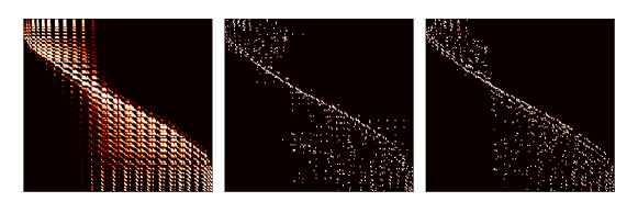
Figure 3: Transport plans of an optimal transport problem. The left, the middle, and the right subfigures are the transportation plans with respect to the initial interior-point solution, the basic solution from Tree-BI, and the optimal BFS after reoptimization. The solution in the left subfigure is generated by Gurobi’s barrier algorithm with the barrier convergence tolerance set to 0.01. In these figures, the brightness of each point at $(i,j)$ represents the amount of grayscale transported from the $i$-th pixel to the $j$-th pixel.

Then, our main experiments will examine the two following questions:

• The crossover procedure in isolation. We use the solutions from Gurobi’s barrier method, with different convergence tolerances, to approximate a solution form the starting method. Based on this solution, we compare TNET, CNET, and Gurobi’s internal crossover stage.

• The overall running time of obtaining an optimal BFS (the time of the crossover procedure coupled with the preceding interior-point or the first-order method). The methods in the comparison include Gurobi’s default method, Cplex’s network simplex algorithm, and the Sinkhorn algorithm augmented with TNET or CNET.

First, we verify (a), comparing different crossover methods. Table 1 compares crossover methods, on optimal transport problems of different scales. Both TNET and CNET show improvements than Gurobi’s crossover in larger instances. Interestingly, TNET exhibits a larger advantage when the given initial interior-point solution has higher accuracy.

Table 1: Crossover procedure comparison of Gurobi’s barrier part (grbBarrier), Gurobi’s crossover part (grbCrossover), CNET-grb and TNET-grb on optimal transport problems generated from MNIST dataset. For each scalarization factor $\alpha$, we test on 10 independent trials and report the geometric average running time (in seconds). The barrier convergence tolerance of the interior-point solution is set to be 1e-8 (the left subtable) and 1e-2 (the right subtable) respectively.

$\alpha$	grbBarrier	grbCrossover	CNET-grb	TNET-grb
1	0.12	0.02	0.02	0.02
2	2.05	0.11	0.14	0.15
3	11.23	0.66	0.64	0.73
4	50.60	8.74	3.78	3.89
5	79.45	29.55	5.70	4.82
6	165.71	98.24	13.53	11.00
7	813.71	809.67	60.75	53.55

$\alpha$	grbBarrier	grbCrossover	CNET-grb	TNET-grb
1	0.10	0.02	0.02	0.02
2	1.70	0.22	0.14	0.15
3	9.19	1.45	0.65	0.74
4	40.69	22.07	3.76	4.12
5	59.83	37.47	5.38	5.04
6	126.31	125.26	14.70	11.69
7	570.56	1015.20	76.75	72.85

Next, we verify (b), comparing the overall running time of different methods. As Table 2 shows, the Sinkhorn+CNET-cpl is slightly better when compared with Sinkhorn+TNET-cpl, and often faster than the network simplex algorithm, particularly in larger-scale scenarios. These advantages also show the potential of combining other first-order methods and network simplex methods, compared with directly running the network simplex method.

Table 2: Total running time comparison of Gurobi’s default method (grbDefault), Cplex’s network simplex method (cplNetSimplex), Sinkhorn+CNET-cpl, and Sinkhorn+TNET-cpl on optimal transport problems generated from MNIST. For each scalarization factor $\alpha$, we test on 10 independent trials and report the geometric average running time (in seconds) and iteration number, which includes all simplex iterations applied, and the push iterations to find a feasible tree BFS (only for TNET).

$\alpha$	grbDefault	cplNetSimplex		Sinkhorn+CNET-cpl		Sinkhorn+TNET-cpl
		time	iterations	time	iterations	time	iterations
1	0.02	0.01	1.6e+03	0.02	1.5e+03	0.02	6.0e+02
2	0.24	0.03	1.2e+04	0.10	1.0e+04	0.17	5.1e+03
3	2.43	0.34	6.1e+04	0.50	3.4e+04	0.84	1.9e+04
4	12.60	2.87	2.0e+05	2.18	9.4e+04	3.38	5.5e+04
5	40.47	4.84	3.0e+05	3.74	1.2e+05	5.78	8.9e+05
6	245.34	12.84	6.3e+05	8.54	2.6e+05	12.50	1.6e+05
7	1521.80	62.10	1.6e+06	37.14	6.1e+05	54.12	3.9e+05

5.1.2 Minimum Cost Flow.

Then, we extend experiments to more general MCF problems. These experiments still use the solutions from early-stopping Gurobi’s barrier method (to approximate the solution of the starting method) and compare our crossover methods with Gurobi’s crossover. We conclude by noting that the potential value of our approach lies particularly in the context of solving large-scale MCF problems in which the solution given by the starting method is of low accuracy, such as outputs of first-order methods in large-scale LP tasks.

We conducted our experiments using benchmark problems from two sources: 1) Hans Mittelmann’s large network-LP benchmark, and 2) networks generated by GOTO. The experiment configurations are the same as the experiments on optimal transport problems in Section 5.1.1.

Table 3 shows that on the large network-LP benchmark dataset, when the given solution is of low accuracy, CNET is much better than Gurobi’s crossover in both overall running time and iteration number. When the given solution is of high accuracy, Gurobi’s crossover has advantages, but both crossover methods are very fast (no more than 10 seconds) in this case. Figure 4 compares CNET with Gurobi’s crossover with the problem scale varying from small to large, in which the largest problems (GOTO_sr with $2^{16}$ nodes) contain over 10 million variables. See the Appendix for the complete tables of the experiments in Table 3 and Figure 4. These results demonstrate the consistent advantages of our crossover methods over Gurobi’s crossover when the given solution from the starting method is of low accuracy (for example, solution of first-order methods). In general, Gurobi’s crossover heavily relies on high-accuracy input solutions while CNET is more stable. This demonstrates that the graph information used in CNET allows for a more robust crossover, which is particularly advantageous when starting from solutions obtained with first-order methods.

Table 3: The comparison of Gurobi’s crossover (grbCrossover) and CNET-grb on large network-LP benchmark dataset. The primal-dual gap of the interior-point solution is set to be 1e-2 and 1e-8. The “GeoAvg Time” and “GeoAvg Iterations” denote the geometric average of running time and iteration number for all problems.

gap	grbBarrier	grbCrossover		CNET-grb
		GeoAvg Time	GeoAvg Iterations	GeoAvg Time	GeoAvg Iterations
1e-2	395.6	68.0	9.8e+05	8.40	4.8e+04
1e-8	581.1	0.52	5.5e+03	4.92	3.9e+04

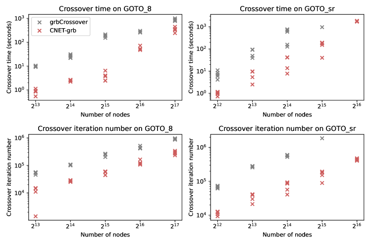
Figure 4: Comparison of Gurobi’s crossover and CNET-grb on GOTO_8 and GOTO_sr with different scales. The barrier convergence tolerance of the interior point solution is set to be 1e-2. The iterations of Gurobi are all the iterations in the crossover (push phase and reoptimization) and the iterations of CNET-grb are all iterations of Col-BI and reoptimization. For each problem scale, we report the results of 5 different generated problems. The time limit is set as 4000 seconds.

5.2 Perturbation Crossover Method

In this subsection, we describe the implementation of the perturbation crossover, in which the perturbed problems are solved by commercial solvers. We then compare it with the solvers’ internal crossover. The experiment setup for the perturbation crossover on one LP problem is as follows:

• Preprocessing. For the given LP problem, we apply Gurobi’s presolve function and obtain a presolved model. In LP solving, the presolve function reduces the problem size by removing redundancies and eliminating variables. It changes the model and advances the realistic solving substantially. Thus, by starting with presolve, we ensure that our experimental framework reflects a realistic and practical optimization setting.

• Barrier method of the solver. We first employ the solver’s barrier method to solve the problem, and the resulting interior-point solution will be used for the perturbation crossover method. We follow the solver’s default tolerance for all problems.

• Perturbation crossover. We adhere to the procedure outlined in the flowchart presented in Figure 2. The initial parameter $\gamma$, for estimating the candidate optimal face, is set to ${1}\mathrm{e}{-3}$. The perturbation vector $p$ on the objective vector, inspired by Theorem 4.3, is calculated on the standard form reformulation and applied more aggressively in practice. For the new artificial variables in the standard form, $p_{i}$ is zero. For other indices $i$, the perturbation is defined as:

  $$p_{i}:=\frac{\xi_{i}}{\|\xi\|_{2}}\cdot\frac{\|P_{X^{-1}\cdot L}(Xc)\|_{2}}{0.01\cdot n\cdot\max\{10^{-6},x_{i}\}},\quad\text{for all }i\in[n].$$ (23)

  Here, $\xi$ is a random vector from a uniform distribution between $0.9$ and $1$, $x=(x_{i})_{i\in[n]}$ represents the interior-point primal solution, and $P_{X^{-1}\cdot L}(c)$ is as defined in 17. Note that 23 is constructed in such a way that 15 is satisfied, particularly when substituting $0.01\cdot n\cdot\max\{10^{-6},x_{i}\}$ to $n\cdot x_{i}$. The reason we use the former expression with dividing by $0.01$ is to intensify the perturbation, a strategy that has been proven more efficient. And taking maximum with $10^{-6}$ mitigates numerical issues with small values of $x_{i}$. In cases where the restricted problem is infeasible, $\gamma$ is reduced by $\gamma\leftarrow\gamma\cdot{1}\mathrm{e}{-5}$, and this step is repeated. The presolve function is activated when solving the perturbed problem.

• Reoptimization. When the relative objective gap between $f_{p}$ (the obective value of the solution of the perturbed restricted problem) and $f_{d}$ (the objective value of the given dual interior-point solution), defined as $\frac{\lvert f_{p}-f_{d}\rvert}{\lvert f_{p}\rvert+\lvert f_{d}\rvert+1}$, is smaller than the default tolerance $\varepsilon:={1}\mathrm{e}{-8}$, then the obtained BFS is considered sufficiently optimal. This tolerance is similar to those of most commercial solvers, like BarConvTol in Gurobi and intpntTolRelGap in Mosek. If the gap exceeds the tolerance, the reoptimization follows by warm starting the simplex method from the BFS.

We measure the running time of the perturbation method by tracking the total elapsed time taken to solve the perturbed model and the time for the following reoptimization phase. The time consumed in determining the feasibility of the problem and in computing the perturbations would be negligible if these processes are integrated within the solvers internally. Consequently, these time components are excluded from the reported running time of the perturbation crossover method.

The first experiment is carried out on the LP relaxation of five max cut packing problems from Bergner et al. (2014). These problems are also collected in the MIPLIB 2017 dataset (Gleixner et al. 2021). For the original mixed integer program, a BFS of the LP relaxation is critical for the subsequent branches and cuts. Table 4 shows the runtime for Gurobi’s barrier method and crossover, and our perturbation crossover, along with the basic information of the problems. As shown in Table 4, the five problems vary not only in scale but also in the dimensions of their optimal faces. While Gurobi is consistently fast in the barrier method part, it tends to consume a considerable amount of time during the crossover phase, especially when the (estimated) dimension of the optimal face is large. When this dimension is large, many linear constraints are inactive for the given interior-point solution, in which case the traditional crossover spends more time identifying an optimal basis. In contrast, our perturbation crossover significantly outperforms Gurobi’s crossover in these cases.

Table 4: The experimental results of $5$ max cut packing problems. “Est. Dim.” denotes the estimated dimension of the optimal face. “grbBarrier”, “grbCrossover”, and “perturbCrossover” show running time (in seconds) of Gurobi’s barrier methods, Gurobi’s crossover methods, and the perturbation crossover method respectively.

Problem	Instance Statistics			grbBarrier	Crossover Time
	Constraints	Variables	Est. Dim.1		grbCrossover	perturbCrossover
graph20-20-1rand	5587	2183	2035	0.01	0.05	0.04
graph20-80-1rand	55107	16263	15912	0.05	2.42	1.11
graph40-20-1rand	99067	31243	30772	0.09	15.84	8.33
graph40-40-1rand	360900	102600	101700	0.41	323.41	50.79
graph40-80-1rand	1050112	283648	282112	1.4	$>$10000	872.07

• For the “optimal face” determined by 13 with $\gamma=1$, the estimated dimension is calculated by $n$ minus the number of
  linear equality constraints.

We then compare the perturbation crossover method with solvers’ internal crossover on Hans Mittelmann’s LPopt Benchmark problems. To validate the perturbation crossover’s effectiveness across different solvers, the same experiments are also done for another widely used commercial solver Mosek (9.2). Different from Gurobi, Mosek applies interior-point method on the homogeneous self-dual model (Andersen 2009) so the iterates follow a different central path. For this reason, Theorem 4.3 cannot directly apply on Mosek. See Table 9 and Table 10 of the Appendix for the complete and comprehensive results of the perturbation crossover based on Gurobi and Mosek.

Figure 5 presents the time for solving the perturbed restricted problem and Gurobi’s internal crossover, as well as the corresponding relative objective gap of the obtained BFS. One can observe that if the goal is to obtain a BFS within default tolerance (achieving a relative objective gap smaller than $10^{-8}$), the obtained BFS is usually already optimal enough except in only 4 instances. Furthermore, the time taken to acquire such a BFS is frequently considerably less than that required by the solver’s own crossover method. It should be mentioned that there is a notable variation in the time for solving the perturbed restricted problem and the time for Gurobi’ internal crossover, which implies in practice if the computing resource is unlimited (which is often seen in practical applications), concurrently running the two crossover methods yields the shortest running time.

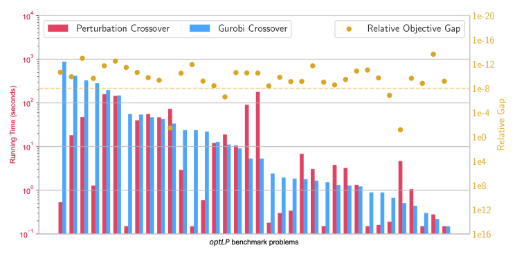
Figure 5: Results of the perturbation crossover and Gurobi’s crossover. The x-axis denotes the benchmark problems, arranged according to the crossover time of Gurobi. The red and blue bars (left y-axis) represent the perturbed model’s solving time and the solver’s original crossover time. The orange dots (right y-axis) represents the relative objective gap between the objective value of the solution of the perturbed restricted problem, and the objective value of the given dual interior-point solution.

Table 5 provides the statistics of the total running time of the perturbation crossover, which includes the time spent on necessary reoptimization phase when the relative objective gap is not within the tolerance. Specifically, we exclude problems that fail in the barrier algorithm (including cases in which Gurobi automatically switches to the homogeneous barrier algorithm) or the barrier algorithm exceeds one hour.

Table 5: Performance statistics of the perturbation crossover method using Gurobi and Mosek on finding a primal BFS within the default tolerance in 36 instances. “Faster” and “Slower” counts how many instances get faster when running in our perturbation crossover methods. “Best per Instance” denotes the minimum of the solver’s original crossover running time or the perturbation crossover method’s running time, to approximate concurrently running the two methods.

Solver	Faster	Slower	GeoAvg Running Time
			Solver’s Crossover	Perturbation Crossover	Best per Instance
Gurobi	19	17	6.83	3.44	1.53
Mosek	15	21	5.16	10.00	2.03

Although the perturbation crossover method is not consistently better than the traditional crossover implemented in solvers, it presents advantages on some problems, especially those used to be considered challenging, such as the 4 instances that Gurobi spends the most time on (see Figure 5). Since Mosek follows a different central path, it makes sense that in Mosek our perturbation crossover does not work as well as the internal crossover, which in turn validates Theorem 4.3. Note that when given sufficient computing resources, running both the traditional crossover and our perturbation crossover methods concurrently can greatly improve computational efficiency and robustness. This is evidenced by the “Best per Instance” column, which exhibits a remarkable speedup — approximately 4 to 5 times faster than Gurobi’s internal crossover alone. Moreover, this technique also applies to Mosek, in which the “Best per Instance” is 2 to 3 times faster than the internal crossover, despite the perturbation crossover itself not outperforming the internal crossover of Mosek. It is important to note that different solvers employ varied parameter setups and algorithms. For example, the barrier methods used by different solvers may follow distinct central paths because of different internal reformulations. As a result, the results in Gurobi and Mosek are different. Despite these discrepancies, the experimental results obtained thus far strongly support the broad applicability and generalizability of the perturbation crossover approach.

Through the experiments comparing our new perturbation crossover method with the internal crossover methods of commercial solvers, we have demonstrated the distinct advantages of our approach. Our crossover method showcases its capability to navigate issues that have historically challenged traditional crossover methods. Moreover, our results reveal the potential for significant speed enhancements when running both the traditional and perturbation crossover methods concurrently. This indicates a promising direction for future optimization methods and tools.

This research is partially supported by the National Natural Science Foundation of China (NSFC) [Grant NSFC-72150001, 72225009, 11831002]. We thank Fangkun Qiu for some valuable experiments in the preliminary version of this paper. We thank the developers from the solver COPT, such as Qi Huangfu, for fruitful discussions. We also thank the anonymous referees for their helpful comments and suggestions, which improved the quality of the manuscript.

6 Complete Numerical Results for Network Problems

MNIST Dataset.

We experiment with the MNIST dataset for the optimal transport problem. This dataset contains 60,000 images of handwritten digits ($28\times 28$ pixels for each), from which an optimal transport problem is generated by first randomly selecting two images and normalizing the sum of their non-zero grayscale values to 1. And then the optimal transport problem is to find an optimal transport plan from one image (as a discrete distribution with $28\times 28$ supports) to the other, with the transport cost defined as the Manhattan distance between the corresponding pixels. To illustrate, transporting the grayscale value from a pixel at location $(7,9)$ to a pixel at index $(13,10)$ incurs a cost of $\|(7,9)-(13,10)\|_{1}=7$ per unit. Furthermore, to expand the problem scale, we artificially increase the image size by a factor of $\alpha$ ($\alpha=1,2,\dots,7$) and create images sized at $28\alpha\times 28\alpha$. The creation is to split each original pixel into $\alpha\times\alpha$ pixels with the same grayscale and normalize as before. The problems of the largest generated group ($\alpha=7$) have on average 60 million variables.

GOTO Problems.

GOTO (Grid on Torus) is one of the hardest problems sets on MCF. We generate our GOTO problems in the same way as Kovács (2015) do. Two types of instances are considered: 1) GOTO_8: sparse network: $m=8n$; 2) GOTO_sr: dense network: $m\approx n\sqrt{n}$, where $m,n$ are the number of arcs and nodes in the network respectively. Note that GOTO problems have been included in Han’s Mittelmann’s Network LP benchmark problems. Since we do experiments on GOTO separately, we ignore all GOTO problems when considering benchmark problems in Table 3 and Table 6.

Table 6: Complete results of Table 3 with a starting interior-point solution of primal-dual gap $1e-2$.

Problem	Node	Arc	grbBarrier	grbCrossover		CNET-grb
				time	iterations	time	iterations
16_n14	16381	261873	31.09	17.1	1.8e+05	6.01	40547
i_n13	8181	739733	24.98	100.8	2.7e+05	7.84	38642
lo10	23728	383578	668.46	295.51	3.2e+05	3.13	55341
long15	32767	753676	812.86	31.54	7.6e+05	3.97	51486
netlarge1	45774	7238591	289.08	345.61	1.7e+06	44.95	89712
netlarge2	39893	1158027	1043.61	41.29	1.2e+06	9.41	69478
netlarge3	38502	4489009	990.27	117.03	3.9e+06	24.50	69326
netlarge6	8000	15000000	774.88	60.26	1.5e+07	19.33	11736
square15	32760	753512	1191.03	39.45	7.6e+05	3.83	53391
wide15	32767	753676	807.88	33.29	7.6e+05	3.86	51486

Table 7: Complete results of Figure 4, GOTO_8

prob	node	arc	grbBarrier	grbCrossover		CNET-grb
				time	iteration	time	iteration
8_13a	8192	65536	6.889	9.18	56895	1.13	15007
8_13b	8192	65536	7.65	9.62	53017	0.85	14448
8_13c	8192	65536	8.96	10.42	45673	0.54	11044
8_13d	8192	65536	6.7	9.53	53242	0.85	1409
8_13e	8192	65536	8.41	10.48	53550	0.93	14943
8_14a	16384	131072	19.22	26.17	108311	2.59	27530
8_14b	16384	131072	24.31	31.39	107992	2.66	29288
8_14c	16384	131072	15.36	21.84	102828	2.21	25294
8_14d	16384	131072	16.79	22.77	100342	2.47	25109
8_14e	16384	131072	21.82	28.15	102061	2.67	28538
8_15a	32768	262144	159.43	209.64	267968	4.07	60136
8_15b	32768	262144	147.3	185.93	262017	3.73	57446
8_15c	32768	262144	177.38	180.61	244905	2.48	44871
8_15d	32768	262144	150.96	152.57	202674	2.44	44258
8_15e	32768	262144	165.39	213.27	262002	6.44	60810
8_16a	65536	524288	130.68	256.75	441523	52.47	112601
8_16b	65536	524288	143.36	255.64	413308	47.15	106872
8_16c	65536	524288	121.97	261.29	422912	53.19	122950
8_16d	65536	524288	129.88	265.76	424800	53.4	123567
8_16e	65536	524288	97.37	300.54	519098	72.13	164305
8_17a	131072	1048576	318.76	773.08	883037	241.51	234596
8_17b	131072	1048576	324.16	872.61	872017	358.82	280343
8_17c	131072	1048576	262.28	796.8	865727	324.32	270919
8_17d	131072	1048576	248.78	892.76	916503	364.76	307621
8_17e	131072	1048576	317.87	1006.43	973954	446.39	339690

Table 8: Complete results of Figure 4, GOTO_sr

prob	node	arc	grbBarrier	grbCrossover		CNET-grb
				time	iteration	time	iteration
sr_12a	4096	262144	9.11	4.13	61338	0.72	9257
sr_12b	4096	262144	11.36	8.45	74070	1.13	12128
sr_12c	4096	262144	9.92	5.91	73286	0.93	12464
sr_12d	4096	262144	8.93	10.95	69361	1.17	12790
sr_12e	4096	262144	8.81	6.98	65259	1.03	10744
sr_13a	8192	741455	24.64	94.02	283373	9.76	39252
sr_13b	8192	741455	22.01	39.54	280913	2.5	21259
sr_13c	8192	741455	28.57	49.29	256458	5.37	30001
sr_13d	8192	741455	29.86	91.38	277565	9.53	39677
sr_13e	8192	741455	29.34	93.98	274104	9.52	41648
sr_14a	16384	2097152	94.78	773.83	596187	41.47	93324
sr_14b	16384	2097152	127.57	694	595303	42.28	87569
sr_14c	16384	2097152	148.57	598.3	602842	41.21	85370
sr_14d	16384	2097152	190.37	127.52	522578	7.74	40602
sr_14e	16384	2097152	248.13	156.52	574786	13.7	56660
sr_15a	32768	5931642	778.51	t	-	203.16	193826
sr_15b	32768	5931642	831.5	t	-	176.6	152008
sr_15c	32768	5931642	1582.08	966.51	1862371	40.06	89170
sr_15d	32768	5931642	758.11	t	-	202.62	190106
sr_15e	32768	5931642	747.57	t	-	195.94	178075
sr_16a	65536	16777216	1715.79	t	-	1796	437039
sr_16b	65536	16777216	1605.52	t	-	1701.88	478398
sr_16c	65536	16777216	1677.75	t	-	1821.62	404442
sr_16d	65536	16777216	1376.29	t	-	1840.97	453485
sr_16e	65536	16777216	1310.3	t	-	1868	420691

7 Complete Numerical Results of Perturbation Crossover Method

Problem set.

Our experiment uses all problems from Hans Mittelmann’s benchmark, excluding the ones that failed or timeout in the barrier algorithm. For example, neos-5251015 (Gurobi changes to the homogeneous algorithm automatically when solving this problem) and physiciansched3-3 (Gurobi solves to a sub-optimal solution and does not return it as the found solution) fail in Gurobi. ns1687037 fails in Mosek (Mosek reports the solution is not found), and ns1688926 fails in both (Gurobi changes to the homogeneous algorithm and Mosek reports the solution is not found). Some problems are too large such that the barrier runs out of time (exceeds one hour), like thk_48, thk_63, and fhnw-binschedule1. Table 9 and Table 10 list the results for all the other problems.

We also note that among all the tested problems, datt256_lp and ex10 are feasibility problems. Therefore, we only solve randomly perturbed problems for these two problems (see Figure 2).

For some instances, the estimated optimal face might be initially infeasible. In that case, we need to decrease $\gamma$ (from 1e-3 to 1e-8, 1e-13, 1e-18, etc) to enlarge the estimated optimal face (see Figure 2). Such cases apply for 5 instances during our experiment, namely cont11, dlr1, set-cover-model, and irish-electricity, for both Gurobi and Mosek, and Linf_520c for Mosek only. For irish-electricity, the first $\gamma$ that makes the candidate optimal face feasible is 1e-13, while for the rest 4 instances, such $\gamma$ is 1e-8.

Table 9: Complete result of the Gurobi part in Table 5. The columns ‘$\text{P}_{\text{bfs}}$ Time’ and ’$\text{PD}_{\text{bfs}}$ Time’ represent the running time needed to obtain an optimal primal BFS within tolerance ${1}\mathrm{e}{-8}$ and the running time needed to obtain primal and dual optimal BFSs.

Problem1	Barrier2	Crossover3	Perturbation Crossover
			Perturb. Time4	Gap5	$\text{P}_{\text{bfs}}$ Time	$\text{PD}_{\text{bfs}}$ Time
s82	143.38	881.19	0.53	2.2e-11	0.53	2329.26
datt256_lp	1.65	415.94	18.19	1.2e-10	18.19	21.66
graph40-40_lp	0.38	327.07	47.15	1.1e-13	47.15	47.34
set-cover-model	132.85	282.14	1.28	2.3e-10	1.28	103.79
woodlands09	6.59	196.39	157.94	1.9e-12	157.94	158.08
a2864	0.23	147.84	144.48	3.2e-13	144.48	229.58
nug08-3rd	0.87	55.7	0.01	3.6e-12	0.01	566.2
savsched1	7.17	54.14	39.8	2.4e-11	39.8	40.13
karted	6.55	46.72	55.6	1.7e-10	55.6	85.48
degme	22.05	42.77	46.8	4.6e-10	46.8	61.51
dlr1	89.66	33.73	73.12	3.4e-02	1511.18	1511.18
neos3	1.83	23.74	2.92	3.2e-11	2.92	1555.26
s100	17.62	23.73	0.06	1.2e-12	0.06	116.6
rmine15	56.06	22.01	0.59	6.4e-10	0.59	187.88
tpl-tub-ws1617	55.08	12.76	12.07	3.7e-09	12.07	58.73
cont11	3.47	11.12	18.92	2.6e-07	841.23	841.23
cont1	2.39	9.05	10.57	2.5e-11	10.57	12.68
ex10	9.51	5.34	90.86	2.9e-11	90.86	90.9
ns1687037	6.91	5.31	178.69	3e-11	178.69	179.13
supportcase19	30.83	2.41	0.18	3.9e-09	0.18	237.49
rail02	41.33	1.95	0.3	1.5e-10	0.3	2969.26
rail4284	26.74	1.84	0.34	7.6e-10	0.34	1.33
Linf_520c	9.86	1.8	6.82	7.2e-10	6.82	6.91
stormG2_1000	88.8	1.66	3.05	1.9e-12	3.05	8.45
square41	1.24	1.52	0.05	9.5e-10	0.05	14.55
qap15	0.57	1.32	3.8	2.7e-09	3.8	22.76
scpm1_lp	21.59	1.28	3.23	3.4e-10	3.23	3.42
pds-100	36.57	1.22	1.33	1.4e-11	1.33	15.6
stp3d	7.92	0.89	0.08	9.4e-12	0.08	81.51
fome13	1.1	0.89	0.16	1.9e-10	0.16	17.2
shs1023	28.42	0.67	0.19	1.4e-07	23.33	23.33
irish-electricity	4.5	0.51	4.68	6.7e-02	54.3	54.3
neos-5052403-cygnet	4.78	0.44	1.06	2.2e-10	1.06	16.75
s250r10	12.81	0.3	0.07	1.5e-09	0.07	1.12
neos	15.06	0.22	0.28	2.4e-14	0.28	0.58
L1_sixm250obs	2.14	0.02	0.05	6.6e-10	0.05	0.06

• The problems are sorted by the running time of the crossover method of the solver.

• Gurobi’s barrier method on the original problem without crossover stage;

• Gurobi’s crossover stage on the original problem;

• The time for solving the perturbed model via Gurobi

• The relative gap between the primal (from the perturbed model) and the dual (from the barrier).

Table 10: Complete result of the Mosek part in Table 5. The columns ‘$\text{P}_{\text{bfs}}$ Time’ and ’$\text{PD}_{\text{bfs}}$ Time’ represent the running time needed to obtain an optimal primal BFS within tolerance ${1}\mathrm{e}{-8}$ and the running time needed to obtain primal and dual optimal BFSs.

Problem1	Barrier2	Crossover3	Perturbation Crossover
			Perturb. Time4	Gap5	$\text{P}_{\text{bfs}}$ Time	$\text{PD}_{\text{bfs}}$ Time
cont11	2.64	2950.6	1070.38	4.5e-01	t6	t
a2864	61.5	555.86	t	nan	t	t
tpl-tub-ws1617	36.24	315.11	5.42	7.3e-07	1300.5	1300.5
datt256_lp	1.38	205.85	3.14	1.8e-12	3.14	4.56
woodlands09	11.41	143.76	159.64	4.2e-09	159.64	t
cont1	3.45	91.08	2534.38	1.79e-12	2534.38	2634.29
nug08-3rd	14.12	69.79	0.01	4.9e-12	0.01	3604.22
savsched1	8.45	60.33	1578.21	1.4e-12	1578.21	2691.28
graph40-40_lp	3.84	42.82	17.59	3.5e-13	17.59	18.58
degme	140.89	38.02	77.35	1.5e-09	77.35	224.08
dlr1	176.46	37.09	249.78	1.3e-01	t	t
karted	96.22	27.58	35.24	3.9e-09	35.24	134.57
set-cover-model	176.38	12.76	1.14	1.1e-10	1.14	15.07
Linf_520c	9.27	7.97	160.39	9.4e-01	1940.92	1940.92
neos3	5.26	6.87	85.89	1.3e-08	494.79	494.79
rmine15	47.85	5.93	3.81	2.4e-10	3.81	1213.63
ex10	7.12	5.41	13.24	2.8e-08	t	t
fome13	4.54	3.95	0.34	9.7e-09	0.34	213.4
s82	45.44	2.38	0.29	1.3e-10	0.29	1225.62
stormG2_1000	26.7	2.3	1.87	4.9e-08	26.86	26.86
supportcase19	9.42	1.96	0.07	1.5e-11	0.07	3343.68
pds-100	33.11	1.32	0.88	2e-10	0.88	114.26
scpm1_lp	20.09	1.3	3.66	6.8e-11	3.66	6.06
qap15	4.58	1.12	1.63	9.4e-14	1.63	6.28
stp3d	6.85	1.06	0.08	8.2e-12	0.08	639.58
square41	4.21	1.04	0.1	5.5e-15	0.1	48.92
rail4284	10.93	0.79	0.72	6.7e-14	0.72	4.57
rail02	46.01	0.61	0.47	1.5e-07	827.25	827.25
physiciansched3-3	22.27	0.58	5.01	4.1e-11	5.01	91.31
neos-5052403-cygnet	3.68	0.53	1.11	4.4e-12	1.11	6.24
neos	9.16	0.48	0.47	2.9e-09	0.47	5.79
shs1023	23.63	0.41	0.14	1.9e-08	30.49	30.49
irish-electricity	7.3	0.38	11.17	8.8e-02	243.57	243.57
s100	4.9	0.12	0.02	3.6e-13	0.02	39.61
s250r10	3.47	0.09	0.05	2.2e-12	0.05	14.51
L1_sixm250obs	3.17	0.02	0.03	1e-10	0.03	0.07

• The problems are sorted by the running time of the crossover method of the solver.

• Mosek’s barrier method on the original problem without crossover stage;

• Mosek’s crossover stage on the original problem;

• The time for solving the perturbed model via Mosek

• The relative gap between the primal (from the perturbed model) and the dual (from the barrier).

• Exceeds time limit: 3600 seconds.

8 A Comparison between Different Perturbation Methods

In this section, we compare different perturbation crossover methods, including an apriori perturbation method, Mehrotra (1991)’s perturbation method, and our method. An apriori perturbation aims at perturbing the cost vector to avoid mutiple optimal solutions, before running the barrier algorithm. Mehrotra (1991)’s method uses an interior-point solution to estimate a better perturbation, while ours added more techniques to control the magnitude of the perturbation and restricted the problem to an estimated optimal face.

Table 11: Differences among perturbation methods.

	Use info from an interior-point solution $x$	Perturbation strategy	Estimate the optimal face
Apriori perturb	No	Random	No
Mehrotra’s method	Yes	Random + info of $x$	No
Our method	Yes	Random + info of $x$ and problem data	Yes

We test these methods in the same problem set as we did in Section 5.2. Mehrotra’s method can be referred to as (2.6) in Mehrotra (1991) and we set the $\epsilon$ to be 1. In Mehrotra’s method, we additionally set the perturbation corresponding to tiny components of the given solution as zero to avoid ill-condition cases. Table 12 shows the significant advantage of our perturbation crossover method.

Table 12: Performance statistics of different perturbation crossover methods: an apriori random perturbation, Mehrotra’s method (Mehrotra 1991), and our method using Gurobi. The goals are to find a primal BFS within precision ${1}\mathrm{e}{-8}$ for all three methods. The numbers of total tested problems are 36 for all three methods. The time limit is set to 500 seconds for this experiment.

	Faster	Slower	Timeout	GeoAvg Time
Apriori perturbation	6	30	5	53.41
Mehrotra’s method	2	34	4	40.75
Our method	19	17	2	3.38

References

- Ahuja et al. (1993) Ahuja RK, Orlin JB, Magnanti TL (1993) Network flows: theory, algorithms, and applications (Prentice Hall).
- Altschuler et al. (2017) Altschuler J, Weed J, Rigollet P (2017) Near-linear time approximation algorithms for optimal transport via Sinkhorn iteration. Advances in Neural Information Processing Systems 30, 1961––1971.
- Andersen (1999) Andersen ED (1999) On exploiting problem structure in a basis identification procedure for linear programming. INFORMS Journal on Computing 11(1):95–103.
- Andersen (2009) Andersen ED (2009) The homogeneous and self-dual model and algorithm for linear optimization. Technical report, Technical Report TR-1-2009, MOSEK ApS.
- Andersen and Andersen (2000) Andersen ED, Andersen KD (2000) The MOSEK interior point optimizer for linear programming: an implementation of the homogeneous algorithm. High performance optimization, 197–232.
- Andersen and Ye (1996) Andersen ED, Ye Y (1996) Combining interior-point and pivoting algorithms for linear programming. Management Science 42(12):1719–1731.
- Applegate et al. (2021) Applegate D, Díaz M, Hinder O, Lu H, Lubin M, O’Donoghue B, Schudy W (2021) Practical large-scale linear programming using primal-dual hybrid gradient. Advances in Neural Information Processing Systems 34:20243–20257.
- Bergner et al. (2014) Bergner M, Lübbecke ME, Witt JT (2014) A branch-price-and-cut algorithm for packing cuts in undirected graphs. Experimental Algorithms: 13th International Symposium, SEA 2014, Copenhagen, Denmark, June 29–July 1, 2014. Proceedings 13, 34–45 (Springer).
- Berkelaar et al. (1999) Berkelaar AB, Jansen B, Roos K, Terlaky T (1999) Basis- and partition identification for quadratic programming and linear complementarity problems. Mathematical Programming 86(2):261–282.
- Bertsimas and Tsitsiklis (1997) Bertsimas D, Tsitsiklis JN (1997) Introduction to linear optimization (Athena Scientific Belmont, MA).
- Bixby (1994) Bixby RE (1994) Commentary—progress in linear programming. ORSA Journal on Computing 6(1):15–22.
- Bixby and Saltzman (1994) Bixby RE, Saltzman MJ (1994) Recovering an optimal LP basis from an interior point solution. Operations Research Letters 15(4):169–178.
- Bowman (1956) Bowman EH (1956) Production scheduling by the transportation method of linear programming. Operations Research 4(1):100–103.
- Charnes and Cooper (1954) Charnes A, Cooper WW (1954) The stepping stone method of explaining linear programming calculations in transportation problems. Management Science 1(1):49–69.
- Chazelle (2000) Chazelle B (2000) A minimum spanning tree algorithm with inverse-Ackermann type complexity. Journal of the ACM (JACM) 47(6):1028–1047.
- CORE-OR (2023) CORE-OR (2023) Clp. URL https://github.com/coin-or/Clp.
- Cuturi (2013) Cuturi M (2013) Sinkhorn distances: Lightspeed computation of optimal transport. Advances in Neural Information Processing Systems 26, 2292–2300.
- Deng et al. (2022) Deng Q, Feng Q, Gao W, Ge D, Jiang B, Jiang Y, Liu J, Liu T, Xue C, Ye Y, et al. (2022) New developments of ADMM-based interior point methods for linear programming and conic programming. arXiv preprint arXiv:2209.01793 .
- Dijkstra et al. (1959) Dijkstra EW, et al. (1959) A note on two problems in connexion with graphs. Numerische Mathematik 1(1):269–271.
- El-Bakry et al. (1994) El-Bakry A, Tapia RA, Zhang Y (1994) A study of indicators for identifying zero variables in interior-point methods. SIAM Review 36(1):45–72.
- Forrest and Goldfarb (1992) Forrest JJ, Goldfarb D (1992) Steepest-edge simplex algorithms for linear programming. Mathematical programming 57(1-3):341–374.
- Galabova and Hall (2020) Galabova I, Hall J (2020) The ‘Idiot’ crash quadratic penalty algorithm for linear programming and its application to linearizations of quadratic assignment problems. Optimization Methods and Software 35(3):488–501.
- Galichon (2018) Galichon A (2018) Optimal transport methods in economics (Princeton University Press).
- Gao et al. (2021) Gao W, Sun C, Ye Y, Ye Y (2021) Boosting method in approximately solving linear programming with fast online algorithm. arXiv preprint arXiv:2107.03570 .
- Ge et al. (2019) Ge D, Wang H, Xiong Z, Ye Y (2019) Interior-point methods strike back: solving the Wasserstein barycenter problem. Advances in Neural Information Processing Systems 32, 6894–6905.
- Glavelis et al. (2018) Glavelis T, Ploskas N, Samaras N (2018) Improving a primal–dual simplex-type algorithm using interior point methods. Optimization 67(12):2259–2274.
- Gleixner et al. (2021) Gleixner A, Hendel G, Gamrath G, Achterberg T, Bastubbe M, Berthold T, Christophel P, Jarck K, Koch T, Linderoth J, et al. (2021) MIPLIB 2017: data-driven compilation of the 6th mixed-integer programming library. Mathematical Programming Computation 13(3):443–490.
- Goldman and Tucker (1956) Goldman AJ, Tucker AW (1956) Theory of linear programming. Linear Inequalities and Related Systems 38:53–97.
- Gurobi Optimization, LLC (2023) Gurobi Optimization, LLC (2023) Gurobi Optimizer Reference Manual. URL https://www.gurobi.com.
- Hanssmann and Hess (1960) Hanssmann F, Hess SW (1960) A linear programming approach to production and employment scheduling. Management Science MT-1(1):46–51.
- Ho et al. (2019) Ho N, Huynh V, Phung D, Jordan M (2019) Probabilistic multilevel clustering via composite transportation distance. The 22nd International Conference on Artificial Intelligence and Statistics, 3149–3157.
- Kovács (2015) Kovács P (2015) Minimum-cost flow algorithms: an experimental evaluation. Optimization Methods and Software 30(1):94–127.
- Li et al. (2020) Li X, Sun D, Toh KC (2020) An asymptotically superlinearly convergent semismooth Newton augmented Lagrangian method for linear programming. SIAM Journal on Optimization 30(3):2410–2440.
- Lin et al. (2020) Lin T, Ma S, Ye Y, Zhang S (2020) An ADMM-based interior-point method for large-scale linear programming. Optimization Methods and Software 36(2-3):1–36.
- Liu and Van Ryzin (2008) Liu Q, Van Ryzin G (2008) On the choice-based linear programming model for network revenue management. Manufacturing & Service Operations Management 10(2):288–310.
- Lu and Yang (2023) Lu H, Yang J (2023) cuPDLP.jl: A GPU implementation of restarted primal-dual hybrid gradient for linear programming in Julia. arXiv preprint arXiv:2311.12180 .
- Maes et al. (2014) Maes C, Rothberg E, Gu Z, Bixby R (2014) Initial basis selection for LP crossover. https://cerfacs.fr/en/sparse-days-meeting-2014-at-cerfacs-toulouse, accessed: 2023–03-24.
- Megiddo (1991) Megiddo N (1991) On finding primal-and dual-optimal bases. ORSA Journal on Computing 3(1):63–65.
- Mehrotra (1991) Mehrotra S (1991) On finding a vertex solution using interior point methods. Linear Algebra and its Applications 152:233–253.
- Mehrotra and Ye (1993) Mehrotra S, Ye Y (1993) Finding an interior point in the optimal face of linear programs. Mathematical Programming 62(1-3):497–515.
- Nesterov and Nemirovskii (1994) Nesterov Y, Nemirovskii A (1994) Interior-point polynomial algorithms in convex programming (SIAM).
- Nguyen (2013) Nguyen X (2013) Convergence of latent mixing measures in finite and infinite mixture models. The Annals of Statistics 41(1):370–400.
- O’donoghue et al. (2016) O’donoghue B, Chu E, Parikh N, Boyd S (2016) Conic optimization via operator splitting and homogeneous self-dual embedding. Journal of Optimization Theory and Applications 169(3):1042–1068.
- Prim (1957) Prim RC (1957) Shortest connection networks and some generalizations. The Bell System Technical Journal 36(6):1389–1401.
- Renegar (2001) Renegar J (2001) A mathematical view of interior-point methods in convex optimization (SIAM).
- Santambrogio (2015) Santambrogio F (2015) Optimal transport for applied mathematicians (Springer).
- Schork and Gondzio (2020) Schork L, Gondzio J (2020) Implementation of an interior point method with basis preconditioning. Mathematical Programming Computation 12(4):603–635.
- Tapia and Zhang (1991) Tapia R, Zhang Y (1991) An optimal-basis identification technique for interior-point linear programming algorithms. Linear algebra and its applications 152:343–363.
- Todd and Ye (1990) Todd MJ, Ye Y (1990) A centered projective algorithm for linear programming. Mathematics of Operations Research 15(3):508–529.
- Wang et al. (2023) Wang H, Ghosal P, Mazumder R (2023) Linear programming using diagonal linear networks. arXiv preprint arXiv:2310.02535 .
- Wolfe (1965) Wolfe P (1965) The composite simplex algorithm. SIAM Review 7(1):42–54.
- Ye (1992) Ye Y (1992) On the finite convergence of interior-point algorithms for linear programming. Mathematical Programming 57(1-3):325–335.