ReSonAte: A Runtime Risk Assessment Framework for Autonomous Systems

Abstract

Autonomous cps are often required to handle uncertainties and self-manage the system operation in response to problems and increasing risk in the operating paradigm. This risk may arise due to distribution shifts, environmental context, or failure of software or hardware components. Traditional techniques for risk assessment focus on design-time techniques such as hazard analysis, risk reduction, and assurance cases among others. However, these static, design-time techniques do not consider the dynamic contexts and failures the systems face at runtime. We hypothesize that this requires a dynamic assurance approach that computes the likelihood of unsafe conditions or system failures considering the safety requirements, assumptions made at design time, past failures in a given operating context, and the likelihood of system component failures. We introduce the ReSonAte dynamic risk estimation framework for autonomous systems. ReSonAte reasons over Bow-Tie Diagrams (BTDs) which capture information about hazard propagation paths and control strategies. Our innovation is the extension of the BTD formalism with attributes for modeling the conditional relationships with the state of the system and environment. We also describe a technique for estimating these conditional relationships and equations for estimating risk based on the state of the system and environment. To help with this process, we provide a scenario modeling procedure that can use the prior distributions of the scenes and threat conditions to generate the data required for estimating the conditional relationships. To improve scalability and reduce the amount of data required, this process considers each control strategy in isolation and composes several single-variate distributions into one complete multi-variate distribution for the control strategy in question. Lastly, we describe the effectiveness of our approach using two separate autonomous system simulations: CARLA and an unmanned underwater vehicle.

I introduction

Autonomous Cyber Physical Systems (cps) are expected to handle uncertainties and self-manage the system operation in response to problems and increase in risk to system safety. This risk may arise due to distribution shifts [1], environmental context or failure of software or hardware components [2]. srm [3] has been a well-known approach used to assess the system’s operational risk. It involves design-time activities such as hazard analysis for identifying the system’s potential hazards, risk assessment to identify the risk associated with the identified hazards, and a system-level assurance case [4] to argue the system’s safety. However, the design-time hazard analysis and risk assessment information it uses is inadequate in highly dynamic situations at runtime. To better address the dynamic operating nature of cps, dynamic assurance approaches such as runtime certification [5], dynamic assurance cases [6], and modular safety certificates [7] have been proposed. These approaches extend the assurance case to include system monitors whose values are used to update the reasoning strategy at runtime. A prominent approach for using the runtime information has been to design a discrete state space model for the system, identity the risk associated with each possible state transition action, then perform the action with the least risk [8].

The effectiveness of dynamic risk estimation has been demonstrated in the avionics [9] and medical [10] domains, but these techniques often encounter challenges with state space explosion which may limit their applicability to relatively low-complexity systems. Also, real-time cps often have strict timing deadlines in the order of tens of milliseconds requiring any dynamic risk assessment technique to be computationally lightweight. Besides, the dynamic risk assessment technique should also take into consideration the uncertainty introduced by the lec because of ood data [11]. Assurance monitors [12, 11] are a type of ood detector often used to tackle the ood data problem. The output of these monitors should be considered when computing the dynamic risk.

Recently, there is a growing interest in dynamic risk assessment of autonomous cps. For example, the authors in [13] have used Dynamic Bayesian Networks to incorporate the broader effect of spatio-temporal risk gathered from road information on the system’s operational risk. To perform dynamic risk assessment of a system with autonomous components, this paper introduces the resonate framework. resonate uses the design-time hazard analysis information to build btd which describe potential hazards to the system and how common events may escalate to consequences due to those hazards. The risk posed by these hazards can change dynamically since the frequency of events and effectiveness of hazard controls may change based on the state of the system and environment. To account for these dynamic events at runtime, resonate uses design-time btd models along with information about the system’s current state derived from system monitors (e.g. anomaly detectors, assurance monitors, etc.) and the operating environment (e.g. weather, traffic, etc.) to estimate dynamic hazard rates. The estimated hazard rate can be used for high-level decision making tasks at runtime, to support self-adaptation of cps.

The specific contributions of this paper are the following. We present the resonate framework and outline the dynamic risk estimation technique which involves design-time measurement of the conditional relationships between hazard rates and the state of the system and environment. These conditional relationships are then used at run-time along with state observations from multiple sources to dynamically estimate system risk. Further, we describe a process that uses an extended btd model for estimating the conditional relationships between the effectiveness of hazard control strategies and the state of the system and environment. To improve scalability and reduce the amount of data required, this process considers each control strategy in isolation and composes several single-variate distributions into one complete multi-variate distribution for the control strategy in question. A key contribution is our scenario specific language that enables data collection by specifying prior distributions over threat conditions and environmental conditions and initial conditions of the vehicle. We implement ReSonAte for an av example in the CARLA simulator [14] and through comprehensive simulations across 600 executions, we show that there is a strong correlation between our risk estimates and eventual vehicular collisions. The dynamic risk calculations on average take only 0.3 milliseconds at runtime in addition to the overhead introduced by the system monitors. Further, we exhibit ReSonAte’s generalizability with preliminary results from an uuv example.

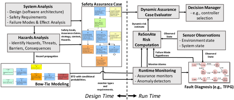
Figure 1: Overview of the steps involved in resonate. Steps performed at design-time/run-time are shown on the left/right.

II Related Work

System health management [15, 16] with model based reasoning have been popularly used for self-adaptation of traditional cps. As discussed in [17], a pre-requisite in these approaches has been that the system has knowledge about itself, its objectives, and its operating environments, including the ability to estimate when the adaption should occur. One way to do this is to estimate the operational risk to the system at runtime. Estimating the runtime risk is more difficult in autonomous systems with lec due to the black box nature of the learning components and their susceptibility to distribution shifts and environmental changes.

Our hypothesis is that we can use btd derived from the system information and static assurance cases and use them to compose the anomaly and the threat likelihoods at runtime, including the likelihood for the failure of lec [11, 12, 18, 1]. btd are graphical models that provide a mechanism to learn the conditional relationships between threat events, hazards, and the success probability of barriers. btd have been proactively used for qualitative risk assessment at design-time [19, 20], and has been recently combined with assurance arguments for operational safety assurance [21, 22].

Although btd have been proactively used for risk assessment, there are several limitations in using them for quantitative risk computations, they are: (1) Static structure - btd have mostly been used as a graphical visualization tool for hazard analysis, and its static structure limits real-data updating which is required for dynamic risk estimation[23], (2) Reliance on domain experts - quantitative risk estimations mostly rely on domain experts to compute the probabilities for the btd events such as threats, and barriers [24], (3) Data uncertainty - introduced because of data non-availability or insufficiency, and expert’s limited knowledge makes it difficult to compute quality probability estimates [25].

Several approaches have been proposed to overcome these limitations and make btd suitable for quantitative risk assessment. Bayesian techniques are one widely used approach that dynamically learns the btd structure from design-time data, and updates the conditional probabilities for its events (e.g., threats, barriers) [26, 27]. Further, [28] transforms a btd into a Bayesian Network where each node of the btd is modelled as a Bayesian Node. The other approach uses techniques such as fuzzy set and evidence theory to address the data uncertainty problems [25, 29]. In this approach, the expert’s knowledge is translated into numerical quantities that are used in the btd. [30] extends btd with petri-nets models and monte-carlo simulations to generate data.

Although prior approaches have made btd suitable for quantitative risk estimation, the design-time hazard information used for risk estimation is inadequate for cps. The main focus of this work is to dynamically estimate risk by fusing design-time information captured in the btd with run-time information about the system and the environment. Additionally, we concentrate on generating large-scale simulation data for conditional probability estimation of the btd events.

III ReSonAte Framework

The goal of the resonate framework is the dynamic estimation of risk based on runtime observations about the state of the system and environment. We define risk as a product of the likelihood and severity of undesirable events, or consequences. Fig. 1 outlines the ReSonAte workflow which is divided into design-time and run-time steps. The design-time steps include System Analysis, Hazard Analysis, Assurance Case Construction, and btd Modeling. Sections III-A1 through III-B provide background information about each of these well-studied techniques. However, our btd formalism described in Section III-B is distinct from existing formalisms with additional model attributes and restrictions for the resonate framework. Sections III-C through III-E introduce the risk calculation equations, the conditional probability estimation process, and the dynamic assurance case evaluation method of the resonate framework respectively.

III-A Background

III-A1 System Analysis

System analysis involves the design-time analysis of the system operation, system faults, the available runtime monitors, and the operating environment such as weather (e.g. rain, snow, fog, etc.), traffic, etc. Thereafter, we perform failure mode analysis to identify the possible component faults and their potential impacts on the safety of the system. Fault propagation paths can be described with the use of an appropriate fault modeling language (e.g. tfpg [31]), and run-time monitors for fault identification can be designed as appropriate. Monitors to detect faults in traditional components have been designed in prior work [32], but monitors for lec are often more complex (e.g. assurance monitors [11]). Alarms raised by these monitors at run-time can then be fed into an appropriate fault diagnosis engine (e.g. the tfpg reasoning engine) to isolate particular fault modes that may be present in the system.

III-A2 Hazard Analysis

Hazard analysis involves the identification of events that may lead to hazardous conditions, implementation of barriers to prevent loss of control over hazard conditions or recovery control after a loss, and estimation of the risk posed by the identified hazards. Guidelines for performing hazard analysis are available in a variety of domains including the ISO 26262 standard [33] for the automotive domain and the FAA System Safety Handbook [34] for the aerospace domain.

III-A3 Assurance Case Construction

An assurance case [4] is a structured argument supported by a body of evidence which shows that system goals will be met in a defined operating environment and is often documented using the gsn [35]. Multiple authors have noted the importance of having ”hazard analysis and risk reduction arguments” within an assurance case [36],[37]. In this work, we only concentrate on the hazard analysis argument of the assurance case, and earlier works [38, 6] can be referred for a more comprehensive dynamic assurance case.

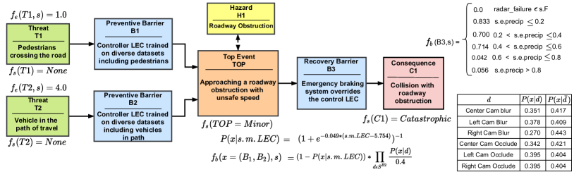
Figure 2: Example Bow-Tie Diagram for autonomous vehicle example ”Roadway Obstruction” hazard created using the ALC Toolchain. Each block includes a brief description and the type of each node is denoted at the top of the block. The equations depicted are described in Section III-B.

III-B Our Contributions: Bow-Tie Formalization & Extensions

btds are used in resonate as the means of describing hazard propagation paths and the control strategies used to prevent that propagation. btd are intended for describing linear propagation and do not have concepts for capturing non-linear causality or complex interactions between events. However, these linear models are sufficient for many hazards commonly encountered by cps such as those demonstrated for the example systems described in Section IV. To perform dynamic risk estimation, the hazard models must also contain information about the expected rate of threat events and the success probability of barriers, both of which may be conditional on the current conditions. In this section, we present a btd formalization which includes this conditional information not captured in existing btd interpretations. Under our formalism, each node has an associated function that is conditional on the state of the system and environment. Before constructing a btd, we assume the following sets have been identified: all potential hazard classes $H$, all events $E$ relevant for hazard analysis, barriers $B$ which may either prevent a loss of control or recover after such a loss has occurred, possible system failure modes $FM$, and event severity classes $SV$. We also assume a function $f_{a}$ which maps each severity class to the maximum acceptable rate of occurrence threshold $f_{a}:SV\rightarrow\mathbb{R}$ has been defined.

For risk calculation, we define the state of the system and the environment as $S=(F,e,m)$ where:

• $F$ is a set of failure modes currently present in the system. $F\subseteq FM$

• $e$ is an n-tuple describing the current environmental conditions where $n$ is the number of environmental parameters that are relevant for risk calculations and each parameter may be continuous or discrete valued.

• $m$ is a k-tuple containing the outputs of runtime monitors in the system where $k$ is the number of such monitors and each monitor may be continuous or discrete valued.

When modeling the environment, the system developer should choose an appropriate level of abstraction based on which environmental parameters are relevant for risk calculation. More environmental parameters may increase the fidelity of the model but also increases the required effort when determining conditional probabilities for events and barriers. It is not required to consider every environmental parameter for all events and barriers. Instead, each event or barrier may be conditional upon a smaller subset of environmental parameters that have the largest impact on that particular event or barrier. Formally, we define a btd as a tuple $(N,C,f_{t},h,f_{d},f_{b},f_{e},f_{s})$ where:

• $N$ is a set of nodes where each node represents either an event $e\in E$ or a barrier $b\in B$.

• $C$ represents a set of directed connections such that $C\subseteq N\times N$. For a given connection $c\in C$, $src(c)$ and $dst(c)$ represent the source and destination of $c$ respectively.

• The tuple $(N,C)$ is a dag representing the temporal ordering of events as well as the barriers which may break this ordering and prevent further propagation of events.

• The function $f_{t}$ gives the type of each node. $f_{t}:N\rightarrow\{event,barrier\}$. Using this function, we let $N_{e}=\{n\in N\ |\ f_{t}(n)=event\}$ and $N_{b}=\{n\in N\ |\ f_{t}(n)=barrier\}$. This gives the following properties: $N_{e}\subseteq E$, $N_{b}\subseteq B$, $N=N_{e}\cup N_{b}$, and $N_{e}\cap N_{b}=\emptyset$.

• $h\in H$ is the hazard class associated with the btd.

• The function $f_{d}$ gives a textual description of each node. $f_{d}:N\rightarrow string$

• $f_{b}$ is a probability function conditional on the state of the system and environment defined for each barrier node. This function represents the probability that the barrier will successfully prevent further event propagation. $f_{b}:N_{b}\times S\rightarrow[0,1]$.

• $f_{e}$ is a function conditional on the state of the system and environment defined for each event node. It gives the expected frequency of the event over a fixed period. The values of this function must be specified for threat events (i.e. root events with no preceding input events), but can be calculated for subsequent events in the diagram as discussed in Section III-C. $f_{e}:N_{e}\times S\rightarrow[0,\inf)$.

• A function $f_{s}$ which maps each event to the appropriate severity class. $f_{s}:N_{E}\rightarrow SV$

btd are often constructed in a chained manner where a consequence event in one section of the btd may serve as a threat or top event in a subsequent section of the same btd. However, such a chained btd can be broken into multiple, single-scope btd where each event has one unique type (i.e. threat, top event, or consequence). As a simplification, resonate operates only on these single-scope btd which satisfy the additional restrictions listed below. Note that the symbol $\Rightarrow$ is used to denote precedence in the graph. That is, given two nodes $a,b\in N$, then $a\Rightarrow b$ states that $a$ precedes $b$ in the btd, but this does not necessitate a direct edge such that $a\rightarrow b$. Instead, there may be any number of intermediate nodes $c_{i}\in N$ such that $a\rightarrow c_{1}\rightarrow c_{2}\rightarrow...\rightarrow c_{n}\rightarrow b$.

• Exactly one event must be designated as the top event, denoted $e_{top}$.

• There must be at least one threat. i.e. $\exists\ t\in N_{e}\ |\ t\Rightarrow e_{top}\land\nexists\ n\in N\ |\ n\Rightarrow t$. We denote the set of all threat events as $N_{t}$.

• There must be at least one consequence. i.e. $\exists\ c\in N_{e}\ |\ e_{top}\Rightarrow c\land\nexists\ n\in N\ |\ c\Rightarrow n$. We denote the set of all consequence events as $N_{c}$.

• All events must be a threat, a top event, or a consequence. i.e. No intermediate events.

• All barriers must lie between a threat and the top event, or between the top event and a consequence. i.e. $\forall\ b\in N_{b}$ either $t\Rightarrow b\Rightarrow e_{top}$ or $e_{top}\Rightarrow b\Rightarrow c$

• No branching or joining of the graph is allowed, except for at the top event.

For the example btd shown in Fig. 2, the type of each event is denoted on the top of the block and we can define the sets $N_{e}$ = $\{T1,T2,TOP,C1\}$ and $N_{b}$ = $\{B1,B2,B3\}$. For each event $e\in N_{e}$, the associated severity class is given by the function $f_{s}(e)$ which is shown under each event block. Each of the threats, $T1$ and $T2$, have been assigned to the ”None” severity class because these events are considered to be common occurrences that do not result in any safety violation by themselves. The top event $TOP$ has been assigned to the ”Minor” severity class since this event can still be mitigated before a safety violation occurs but mitigation requires the aebs to override the primary LEC controller. Finally, the consequence $C1$ has been assigned to the ”Catastrophic” severity class since this event is a safety violation and may result in significant damage to the system or environment.

The conditional functions $f_{e}$ and $f_{b}$ are shown near their respective nodes in Fig. 2. The functions $f_{e}(T1,\textbf{s})$ and $f_{e}(T2,\textbf{s})$ give the expected frequency of threats $T1$ and $T2$ in units of expected number of occurrences per minute, and their values were measured for our simulator configuration described in Section IV. The probability function for barriers $B1$ and $B2$, $f_{b}$(x = (B1,B2), s), shows how these barriers are dependent on both the continuous-valued output from the assurance monitor and on the binary state of other monitors. A sigmoid function, $P(x|\textbf{s}.m.LEC)$, is used to capture the conditional relationship with the assurance monitor output. Finally, $f_{b}(B3,\textbf{s})$ shows how barrier $B3$ is less likely to succeed as the precipitation increases and will not function in the case of a radar failure. Section III-C explains the generic process for conditional probability estimation and Section IV-A4 provides more detail on the functions in this btd.

III-C Run-time Risk Computation

Each btd includes functions describing the conditional frequency for all threat events and the conditional probability of success for all barrier nodes. However, the likelihood of each consequence is necessary to estimate the overall level of risk for the system. These probabilities can be calculated by the propagation of the initial threat rates through the btd. When a particular event occurs, barrier nodes reduce the probability that the event will continue to propagate through the btd based on the following equation:

$$R(e_{2}|s)=R(e_{1}|s)P(\overline{b_{1}}\land\overline{b_{2}}\land...\land\overline{b_{n}}|s)$$

$$assume\ a\perp b\ \forall\ a,b\in\{b_{1},b_{2},...,b_{n}\}\ |\ a\neq b$$

$$R(e_{2}|s)=R(e_{1}|s)[\Pi_{i=1}^{n}P(\overline{b_{i}}|s)]$$ (1)

where $e_{1},e_{2}\in N_{e}$ and $b_{i}\in N_{b}$ such that $e_{1}\rightarrow b_{1}\rightarrow b_{2}\rightarrow...\rightarrow b_{n}\rightarrow e_{2}$. $R(e_{i}|s)$ represents the frequency of event $e_{i}$ given state $s$. Eq. 1 makes the assumption that no barriers share any common failure modes and that the effectiveness of each barrier is independent from the outcome of other barriers. Similarly, $P(\overline{b_{i}}|s)$ represents the probability that barrier $b_{i}$ will fail to prevent event propagation given state $s$, i.e. $P(\overline{b_{i}}|s)$ = $1-P(b_{i}|s)$. Letting $S$ represent the set of all states we are concerned with, then we can calculate the overall frequency of $e_{2}$ as $R(e_{2})=\Sigma_{s\in S}[R(e_{2}|s)P(s)]$ where $P(s)$ is the probability of each particular state $s\in S$. As discussed in the btd formalization in Section III-B, no joining or splitting of paths is allowed in a btd with the exception of the top event $e_{top}$. We treat the top event as a summation operation for all incoming edges, i.e. any threat event may independently cause a top event if the associated barriers are unsuccessful. All outgoing edges from the top event are treated as independent causal chains, i.e. any potential consequence may occur from a top event, independent of other consequences in the btd. The probability for the top event can be calculated as:

$$R(t^{top})=\Sigma_{s\in S}[R(t|s)P(s)[\Pi_{i=1}^{n}P(\overline{b_{i}}|s)]]$$

$$R(e_{top})=\Sigma_{t\in N_{t}}R(t^{top})$$ (2)

where $R(e_{top})$ is the frequency for the top event and $P(t^{top})$ represents the contribution of each threat $t$ to this rate after passing through any intermediate prevention barriers $b_{i}\in N_{b}$ such that $t_{i}\rightarrow b_{1}\rightarrow b_{2}\rightarrow...\rightarrow b_{n}\rightarrow e_{top}$. Finally, the probability of each consequence can be calculated with:

$$R(c_{i})=R(e_{top})\Sigma_{s\in S}[P(s)[\Pi_{i=1}^{n}P(\overline{b_{i}}|s)]]$$ (3)

where $R(c_{i})$ is the frequency of consequence $c_{i}\in N_{c}$ after passing through any recovery barriers $b_{i}\in N_{b}$ such that $e_{top}\rightarrow b_{1}\rightarrow b_{2}\rightarrow...\rightarrow b_{n}\rightarrow c_{i}$.

If the state is not known uniquely, then each potential state $\textbf{s}\in S$ must be enumerated and a probability function $P(\textbf{s})$ must be assigned such that $\Sigma_{\textbf{s}\in S}P(\textbf{s})=1$. At design-time when only the expected distributions of the state variables are known, this state probability function is typically calculated as a product of the probability mass functions (or probability density functions for continuous variables) of each individual state variable. Recall that for resonate the state $S$ is restricted to only those variables which have a conditional impact on the functions contained in the btd and thus not all state variables describing the system must be considered in this calculation. When the system is deployed at run-time, observations about the current state can be used to refine the set of prior probabilities $P(s)$ and dynamically calculate current risk values. The equations outlined here use a discrete treatment of probability, but continuous distributions can be used as well where summation operations are replaced by an appropriate integration. If the state can be identified uniquely to a particular state $\textbf{s}_{0}\in S$, then we can assign $P(\textbf{s}_{0})=1$ and simplify the risk equations. For example, we could calculate the rate of occurrence for events $TOP$ and $C1$ which are part of the btd $B$ shown in Fig. 2 using the following equations:

$$R(TOP|s_{0}) =B.f_{e}(T1,s_{0})*(1-B.f_{b}(B1,s_{0}))$$

$$+B.f_{e}(T2,s_{0})*(1-B.f_{b}(B2,s_{0}))$$

$$R(C1|s_{0})=R(TOP|s_{0})*[1-B.f_{b}(B3,s_{0})]$$ (4)

III-D Estimating Conditional Relationships

III-D1 Conditional Relationships

In resonate, both the rate of occurrence of events and the effectiveness of barriers may be conditionally dependent on the state including system failure modes, runtime monitor values, and environmental conditions. For each of these categories, it is necessary to identify the factors which should be examined for their impact on this conditional relationship. A failure analysis should be performed using an appropriate failure modeling language as discussed in Section III-A1. Similarly, the environmental parameters relevant to the system must be identified and the operating environment defined in terms of bounds and expected distributions of these parameters. We assume the environmental conditions are known uniquely and provided to resonate. Monitor values that may impact the conditional relationships should also be identified.

For some nodes in a btd it may be possible to analytically derive the appropriate conditional relationship with each state variable, but often this relationship must be inferred from data. In this section, we consider a generic threat to the top event chain with a single barrier described as $t\rightarrow b\rightarrow e_{top}$. The contribution to the rate of the top event $e_{top}$ from this singular threat $t$ with a single barrier $b$ is shown in Eq. 5. Normally, multiple threats can lead to the top event and the contribution of all threats must be considered as described in Eq. 2. However, if all other threat conditions can be eliminated, then the top event may only occur as a result of threat $t$. In this case, the probability of success for barrier $b$ can be calculated as a function of the ratio of frequencies between the top event and threat $t$ shown in Eq. 6. This approach can also be used for threats with multiple associated barriers by considering each barrier in isolation since individual barriers are assumed to be independent in Eq. 1.

$$R(e_{top}^{t}|\textbf{s})=R(t|\textbf{s})*(1-P(b|\textbf{s}))$$ (5)

$$R(t_{j}|\textbf{s})=0\ \forall\ t_{j}\in N_{t}\ |\ t_{j}\neq t\rightarrow R(e_{top}|\textbf{s})=R(e_{top}^{t}|\textbf{s})$$

$$P(b|\textbf{s})=1-[R(e_{top}|\textbf{s})/R(t|\textbf{s})]$$ (6)

We isolate individual threats in simulation using a custom sdl, described in Section III-D2, to generate scenarios where only the one threat of interest is allowed to occur and all other possible threats are eliminated. Each time the threat $t$ is encountered, the top event $e_{top}$ may either occur or not occur. If the top event does not occur, then the associated barrier $b$ was successful - i.e. prevented hazard propagation along this path. Otherwise, the barrier was unsuccessful. Since the occurrence of a threat is a discrete event that results in a boolean outcome (i.e. top event does/does not occur), the barrier effectiveness can be modeled as a conditional Binomial distribution where the probability of barrier success is dependent on the ratio of top event frequency to threat frequency as shown in Eq. 6.

For each barrier $b$ in the btd, any state variables which are likely to impact the conditional frequency or probability of that node should be identified, and we denote this reduced set of state variables as $S^{b}$. For discrete state variables (e.g., presence or absence of a particular fault condition, urban/rural/suburban environment, etc.), this ratio can be estimated using Laplace’s rule of succession [39] as shown in Eq. 7 where $n_{s_{i}=a}$ is the number of scenes where the state variable $s_{i}$ had the desired value $a$ and $k_{s_{i}=a}$ is the number of such scenes where the top event also occurred. This equation can be applied for each of the possible values of the state variable $s_{i}$ to estimate the discrete probability distribution $P(b|s_{i})$, and the process can then be repeated for each relevant state variable $s_{i}\in S^{c}$. Eq. 8 can be used to fuse the estimated distributions of each individual state variable into one multivariate distribution $P(b|\textbf{s})$. Similar to Naive Bayes classifiers, this equation assumes each of the state variables $s_{i}$ are mutually independent conditional on the success of barrier $b$. If a stronger assumption is used that the state variables in $S^{b}$ are mutually independent, then the term $\Pi_{j=0}^{m}[P(s_{j})]P(s_{0}s_{1}...s_{m})^{-1}$ reduces to 1 as was the case for all of the probabilities estimated in our examples. For each continuous state variable $s_{j}$ (e.g. output of an assurance monitor), maximum likelihood estimation was used in place of Eq. 7 to estimate $P(b|s_{j})$. Similarly, Eq. 8 can be revised for continuous values by replacing the probability mass functions $P(s_{j})$ with probability density functions $p(s_{j})$.

$$P(b|s_{i}=a)=1-\frac{k_{s_{i}=a}+1}{n_{s_{i}=a}+2}$$ (7)

$$P(b|\textbf{s})=\frac{P(s_{0},s_{1},...,s_{m}|b)P(b)}{P(s_{0},s_{1},...,s_{m})}$$

$$assume\ s_{j}\perp s_{k}\ |\ b\ \forall\ s_{j},s_{k}\in S^{b}\ |\ s_{j}\neq s_{k}$$

$$P(b|s_{0},s_{1},...,s_{m})=\frac{P(b)\Pi_{j=0}^{m}P(s_{j}|b)}{P(s_{0},s_{1},...,s_{m})}$$

$$P(b|s_{0},s_{1},...,s_{m})=\frac{\Pi_{j=0}^{m}P(b|s_{j})P(s_{j})}{P(b)^{m-1}P(s_{0}s_{1}...s_{m})}$$ (8)

While the conditional probability estimation process is outlined here for prevention barriers, it may be modified for recovery barriers by replacing occurrences of any threats t with the top event $e_{top}$ and replacing occurrences of the top event with each consequence of interest.

III-D2 Scenario Description Language

Description and generation of scenarios that cover the full range of expected operating environments is an important aspect for the design of cps. Several domain-specific sdl such as Scenic [40] and MSDL [41] with probabilistic scene generation capabilities are available. While these languages have powerful scene generation capabilities, they are targeted specifically at the automotive domain. We have developed a simplified sdl using the textX [42] meta language to generate varied scenes for multiple domains including our av and uuv systems.

⬇

scene sample {

type string

type int

entity town_description{

id:string

map:string }

entity weather_description{

cloudiness: uniform

precipitation: uniform

precipitation_deposits: uniform }

entity uniform{

low: int

high: int }

}

Figure 3: This listing shows a fragment of a CARLA scene description that was generated using our sdl written in textX meta language.

A fragment of the scene description for the CARLA av example is shown in Fig. 3. A scene S = {$e_{1}$,$e_{2}$,…,$e_{i}$} is described as a collection of entities (or set points), with each entity representing information either about the ego vehicle (e.g., type, route, etc.), or the operating environment (e.g., weather, obstacle). Further, each of these entities has parameters whose value can be sampled using techniques such as Markov chain Monte Carlo to generate different scenes in the simulation space. The larger the number of sampling, the wider is the simulation space coverage. For the av example, our scene was defined as S = {town_description, weather_description, av_route}. While the parameters of town_description and av_route remained fixed, the parameters of weather_description such as cloud, precipitation, and precipitation deposits were randomly sampled to take a value in [0,100]. We generated 46 different CARLA scenes by randomly sampling the weather parameters, a few of which were used for estimating the conditional relationships.

Currently we perform unbiased sampling to generate each scenario, then use the resulting unbiased dataset for the probability calculations described in Section III-D. This approach proved sufficient for the example systems described in Section IV. However, these systems are prototypes where consequences occur relatively often. For more refined production systems, consequences do not typically occur under nominal operation but instead are often the result of rare combinations of adverse operating conditions and/or system failure modes. This is an example of the long tails problem where the probability of observing this undesired system behavior is low if unbiased random sampling is used. In future work, guided sampling of the state space (e.g. [43]) can be used to better observe these rare events and perform conditional probability estimation with the resulting biased dataset.

III-E Dynamic Assurance Case Evaluation

srm [3] is a common technique used in the system safety assurance process which involves identification of potential hazards, analysis of the risks posed by those hazards, and reduction of these risks to acceptable levels. The amount of risk remaining after risk control strategies have been implemented is known as the residual risk. An appropriate assurance argument pattern, such as the alarp pattern outlined by Kelly [35], is often used to document the means used for risk reduction and show that the estimated levels of residual risk are within tolerable bounds. With traditional srm techniques, residual risk estimates are static results of design-time analysis techniques. However, using the risk estimated by resonate the residual risk for each hazard can be updated dynamically at run-time and the associated goal in the assurance argument can be invalidated if the risk exceeds a predefined threshold. When this risk threshold is violated, contingency plans can be enacted to place the system in a safe state. For example, stopping the AV or surfacing the UUV are simple contingency actions used for the example systems described in Section IV. The risk scores produced by resonate may also be used in assurance case adaptation techniques such as Dynamic Safety Cases [6] or ENTRUST [44].

IV Evaluation

We evaluate resonate using an av example in the CARLA simulator [14] and show its generalizability with preliminary results from an uuv example [45]. The experiments in this section were performed on a desktop with AMD Ryzen Threadripper 16-Core Processor, 4 NVIDIA Titan Xp GPU’s and 128 GiB memory.

(a) Screenshot from CARLA simulator.

(b) Top-down view of BlueROV2.

Figure 4: Screenshots from each autonomous system simulation. Fig. 4(a) shows an image from the forward-looking camera of the av as it navigates through the city. Fig. 4(b) shows a top-down view of the uuv where the vehicle (trajectory shown as a green line) is inspecting a pipeline (thick blue line) until an obstacle (grey box) is detected by the forward-looking sonar and the vehicle performs an avoidance maneuver.

IV-A Autonomous Ground Vehicle

IV-A1 System Overview

Our first example system is an autonomous car which must safely navigate through an urban environment while avoiding collisions with pedestrians and other vehicles in a variety of environmental and component failure conditions. The architecture of our av, shown in Fig. 5, relies on a total of 9 sensors including two forward-looking radars, three forward-looking cameras, a gps receiver, an imu, and a speedometer. The ”Navigation” lec, adapted from previous work [46], produces waypoints for the desired position and velocity of the vehicle at a sub-meter granularity using a neural network for image processing along with higher-level information about the desired route provided by a map. These waypoints are passed to the ”Motion Estimator” which computes throttle and steering angle error between the current and desired waypoints. The Motion Estimator also serves as a supervisory controller which will override the primary Navigation component if an alarm is sent by the aebs safeguard component. This aebs component will raise an alarm when the vehicle safe stopping distance, estimated based on the current vehicle speed, exceeds the distance returned by the radars indicating that the av is approaching an object at an unsafe speed. Finally, the output of the Motion Estimator is sent to two PID controllers which generate appropriate steering, throttle, and brake control signals.

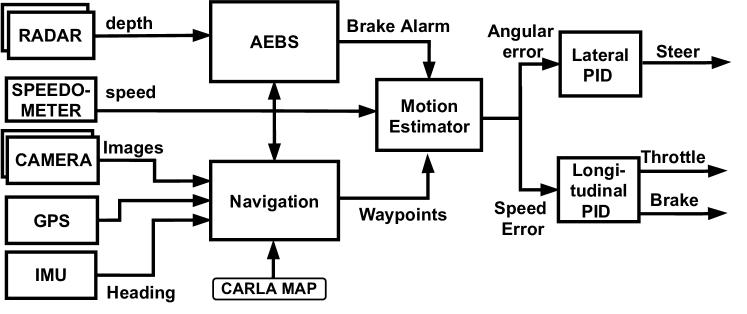
Figure 5: A block diagram of our av example in CARLA simulation.

IV-A2 System Analysis

We start with the analysis of the av system and its operating environment (e.g., weather, traffic, etc). As the av primarily uses a perception lec, parameters such as weather conditions (e.g., cloud spread, precipitation level, and precipitation deposit level), high brightness, and camera related faults such as blur and occlusion influenced the control actions generated by the LEC controller. To detect the camera faults and adverse operating conditions, we have designed several monitors. Each of the three cameras is equipped with OpenCV based blur and occlusion detectors to detect image distortions. The blur detector uses the variance of the laplacian [47] to quantify the level of blur in the image where a high variance indicates that the image is not blurred, while a low value ($<$30) indicates the image is blurred. The occlusion detector is designed to detect continuous black pixels in the images, with the hypothesis that an occluded image will have a higher percentage of connected black pixels. In this work, a large value ($>$15%) of connected black pixels indicated an occlusion. The blur detector has an F1-score of 99% and the blur detector has an F1-score of 97% in detecting the respective anomalies.

Additionally, we leverage our previous work [11] to design a reconstruction based $\beta$-VAE assurance monitor for identifying changes in the operating scenes such as high brightness. The $\beta$-VAE network has four convolutional layers $32/64/128/256$ with (5x5) filters and (2x2) max-pooling followed by four fully connected layers with $2048$, $1000$, and $250$ neurons. A symmetric deconvolutional decoder structure is used as a decoder, and the network uses hyperparameters of $\beta$=1.2 and a latent space of size=100. This network is trained for 150 epochs on 6000 images from CARLA scenes of both clear and rainy scenarios. The reconstruction mean square error of the $\beta$-VAE is used with Inductive Conformal Prediction [48] and power martingale [49] to compute a martingale value. The assurance monitor has an F1 score of 98% in detecting operating scenes with high brightness. Further, tfpg models for the identified camera faults were constructed, but the tfpg reasoning engine was not used since the available monitors were sufficient to uniquely isolate fault conditions without any additional diagnostic procedures.

IV-A3 Hazard Analysis and btd Modeling

For our av example, we consider a single hazard of a potential collision with roadway obstructions. The potential threats for this hazard were identified to be pedestrians crossing the road (T1), and other vehicles in the av’s path of travel (T2). The top event was defined as a condition where the av is approaching a roadway obstruction with an unsafe speed. The primary lec is trained to safely navigate in the presence of either of these threats and served as the first hazard control strategy for both threat conditions, denoted by prevention barriers B1 and B2. Finally, the aebs served as a secondary hazard control strategy denoted by the recovery barrier B3. The btd shown in Fig. 2 was constructed based on these identified events and control strategies. For full-scale systems, the btd construction process will usually result in the identification of a large number of events and barriers modeled across many btd. For our example, we have restricted our analysis to these few events and barriers contained in a single btd.

IV-A4 Conditional Relationships

Here we consider the barrier node B2 in Fig. 2 as an example for the probability calculation technique described in Section III-D. Barrier B2 is part of the event chain $T2\rightarrow B2\rightarrow TOP$ and describes the primary control system’s ability to recognize when it is approaching a slow-moving or stopped vehicle in our lane of travel (T2) too quickly and slow down before control of the roadway obstruction hazard (H1) is lost. To isolate barrier B2, simulation scenes were generated using our sdl where T2 was the only threat condition present but all other system and environmental parameters were free to vary. It is important for these scenes to cover the range of expected system states and environmental conditions since the resulting dataset is used to estimate the conditional probability of success for barrier B2. A total of 300 simulation scenarios were used for estimating the probability of barrier B2. As a convenience for our example, the threat (T2) was set to occur once during each scene, regardless of other state parameters, which allows the denominator of this ratio to be set as $R(T2|\textbf{s})=1$ occurrence per scene.

As perception lec is the primary controller, the success rate of barriers B1 and B2 will be dependent on the image quality. The image quality will in turn be dependent on image blurriness, occlusion, and environmental conditions. While the level of blur and occlusion for each camera is a configurable simulation parameter, our example system is not provided this information and instead relies on blur and occlusion detectors for each of the three cameras as discussed in Section IV-A2. Each detector provides a boolean output indicating if the level of blur or occlusion exceeds a fixed threshold. The primary lec is also susceptible to ood data, and an assurance monitor was trained for this lec to detect such conditions.

This results in barrier $B2$ being dependent on a total of 7 state-variables described as the set $S^{B2}$. For the 6 boolean variables, Laplace’s rule of succession shown in Eq. 7 was applied to the simulation dataset resulting in probability table in the lower-right section of Fig. 2. A sigmoid function was chosen to model the conditional relationship with the continuous assurance monitor output. Maximum likelihood estimation was used to produce the function $P(x|\textbf{s}.m.LEC)$ shown in Fig. 2 where $\textbf{s}.m.LEC$ represents the output of the lec assurance monitor. Each of these single variable functions was combined into the multivariate conditional probability distribution $f_{b}(B2,\textbf{s})$ using Eq. 8. Note that the lec was observed to be similarly effective in identifying pedestrians and vehicles, and a simplifying assumption was made to use the same conditional probability function for both barriers B1 and B2 given by function $f_{b}$(x = (B1,B2), s) in Fig. 2.

The aebs described by barrier B3 is independent of the camera images and relies on the forward looking radar. The level of noise in our simulated radar sensor increased with increasing precipitation levels, indicating that the effectiveness of barrier B3 would likely decrease as precipitation increased. Also, failure of the radar sensor may occur on a random basis which reduces the effectiveness of the aebs to zero. A similar conditional estimation process as used for B2 was applied here to calculate the function $f_{b}(B3,\textbf{s})$ shown in Fig. 2.

IV-A5 Results

To validate the resonate framework, the av was tasked to navigate 46 different validation scenes that were generated using our sdl. In these scenes, the weather_description parameters of cloud (c), precipitation (p), and precipitation deposits (d) were varied in the range [0,100]. Other adversities were synthetically introduced using OpenCV including increased image brightness, camera occlusion (15%-30% black pixels), and camera blur (using 10x10 Gaussian filters). During each simulation, the ReSonAte’s risk calculations continuously estimate the hazard (or collision) rate $h(t)$ based on changing environmental conditions, presence of faults, and outputs from the runtime monitors. The frequency of the risk estimation can be selected either based on the vehicle’s speed, environmental changes, or available compute resources. In our experiments, we estimate the risk every inference cycle.

Figure 6: ReSonAte estimated collision rate and likelihood of collision for 2 validation scenes. (Top) Scene1 - nominal scene with good weather and an intermittent occlusion fault for left and center cameras. (Bottom) Scene2 - initially nominal scene until 27 seconds when image brightness is increased. A collision occurs at 38 seconds denoted by the vertical dotted line.

Fig. 6 shows the estimated collision rate and the likelihood of collision as the av navigates 2 validation scenes. The occurrence of a collision can be described as a random variable following a Poisson distribution where the estimated collision rate is the expected value $\lambda$. The likelihood of collision can then be computed as ($1-e^{-\lambda\cdot t}$), where $\lambda$ is the estimated collision rate and $t$ is the operation time which is fixed to 1 minute in our experiments.

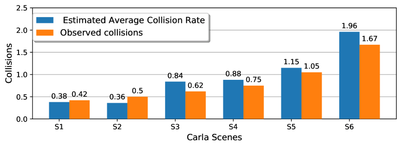
Figure 7: ReSonAte estimated average collision rate vs. observed collisions compared across 6 validation scenes. The results are averaged across 20 simulation runs for each scene. Each subsequent scene represents increasingly adverse weather and component failure conditions.

Fig. 7 shows the estimated average collision rate plotted against the observed collisions for 6 validation scenes described in the figure caption. The estimated average collision rate is calculated as $\frac{\int_{T_{1}}^{T_{2}}h(t)\,dt}{T_{2}-T_{1}}$, where, h(t) is the estimated collision rate, $T_{1}$ = 0 and $T_{2}$ = 1 minute for our simulations. A moving average is used to smooth the estimated collision rate and a window size of 20 was selected to balance the desired smoothing against the delay incurred by the moving average. An overall trend in the plot shows a strong correlation between the actual and the estimated collisions. Also, a visible trend is that the collision rate changes with the weather patterns, increasing for adverse weather conditions (S5-S6). However, the estimated risk tends to slightly overestimate when the collision rate is greater than 1.0.

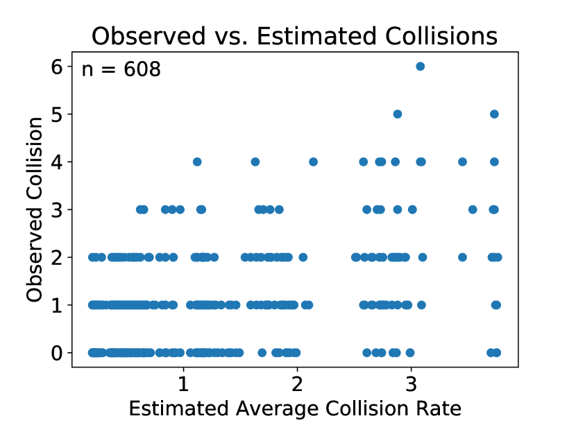
(a) Validation data scatter plot.

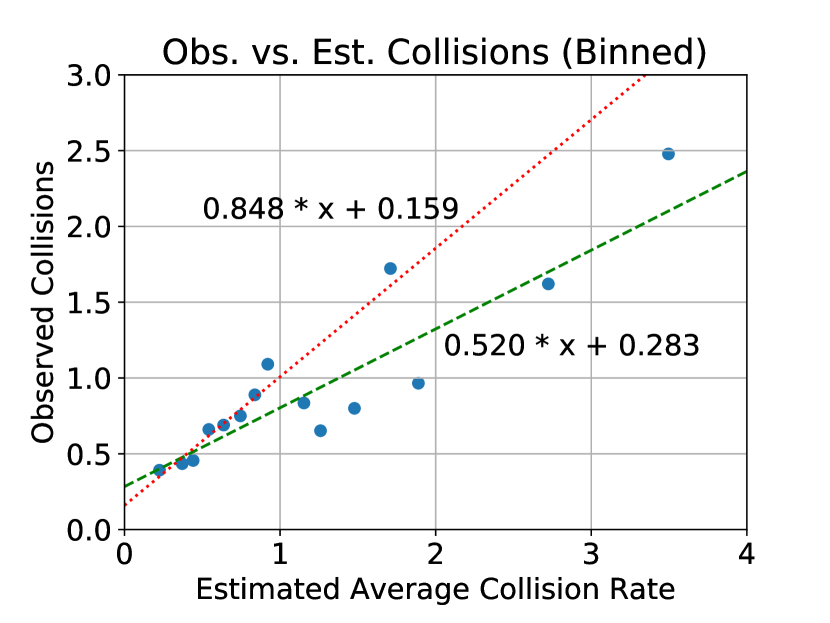
(b) Binned validation data.

Figure 8: Results from validation scenes for the resonate framework. Each data point shown in Fig. 8(a) represents the outcome of one simulated scene with the actual number of collisions observed plotted against the estimated average collision rate. These same data points have been divided into bins and averaged in Fig. 8(b), along with two least-squares fit trend lines.

Further, each of the 608 data points shown in Fig. 8(a) represents the outcome of one simulated scene with the actual number of collisions plotted against the average collision rate estimated by resonate. Since the occurrence of a collision is a probabilistic event, there is significant variation in the actual number of collisions observed in each scene. Using our dynamic rate calculation approach, the rate parameter $\lambda$ of the Poisson distribution changes for each scene as shown on the x-axis of Fig. 8(a). Maximum likelihood analysis was used to compare our dynamic approach against a static, design-time collision rate estimate where $\lambda$ is fixed for all scenes. The observed average collision rate across all scenes was found to be 0.829 collisions per minute. Using this static $\lambda$ value gave a log likelihood of -740.7 while the dynamically updated $\lambda$ resulted in a log likelihood of -709.8 for a likelihood ratio of 30.9 in favor of our dynamic approach. Note that the static collision rate used here is a posterior estimate calculated from the true number of collisions observed. Any static risk estimate made without this post facto knowledge would result in a lower likelihood value and further increase the gap between the dynamic and static approaches.

To better show the correlation between estimated and actual collisions, the same data points have been divided into bins and averaged in Fig. 8(b) along with two least-squares fit trend lines. The dashed green trend line shows a linear fit to the complete data set while the dotted red line shows a linear fit to only those data points where the average estimated collision rate was less than or equal to 1.0. Both trend lines show a strong positive correlation between the estimated collision rate and the number of observed collisions, but the dotted red line more closely resembles the desired 1-to-1 correspondence between estimated and actual collisions (i.e. slope of 1). These results indicate that our dynamic risk calculation tends to over-estimate when the estimated collision rate is greater than 1.0.

	GPU		CPU
System Configuration	Util (%)	Mem (%)	Util (%)	Mem (%)	Execution Time (s)
LEC only	14.3	47.2	17.6	10.4	0.024
LEC + Runtime Monitors	14.7	86.5	18.5	10.5	0.217
LEC + Monitors + ReSonAte	16.1	87.0	18.7	10.4	0.218

TABLE I: Resource requirements and execution times for different configurations of the system. Average values computed across 20 simulation runs.

Table I shows the resource requirements and execution times for system with different configurations. As seen from the shaded columns, the additional sensors, and system monitors, particularly the resource intensive $\beta$-VAE monitor, increases the GPU memory used by $\sim$ 40% and execution time by $\sim$ 0.2 seconds. However, the ReSonAte risk calculations require minimal computational resources taking only 0.3 milliseconds.

IV-B Unmanned Underwater Vehicle

In this section we discuss the primary results of applying ReSonAte to a uuv testbed based on the BlueROV2 [45] vehicle. The testbed is built on the ROS middleware [50] and simulated using the Gazebo simulator environment [51] with the uuv Simulator [52] extensions.

IV-B1 System Overview and btd Modeling

In this example, the uuv was tasked to track a pipeline while avoiding static obstacles (e.g., plants, rocks, etc.) as shown in Fig. 4(b). The uuv is equipped with 6 thrusters, a forward looking sonar (FLS), 2 side looking sonars (SLS), an IMU, a GPS, an altimeter, an odometer, and a pressure sensor. The vehicle has several ROS nodes for performing pipe tracking, obstacle avoidance, degradation detection, contingency planning, and control. Additional contingency management features such as thruster reallocation, return-to-home, and resurfacing are available. The uuv uses the SLS along with the FLS, odometry, and altimeter to generate the HSD commands for pipe tracking and obstacle avoidance. The degradation detector is an lec which employs a feed-forward neural network to detect possible thruster degradation based on thruster efficiency information. This lec sends information to the contingency manager including the identifier of the degraded thruster, level of degradation, and a value measuring confidence in the predictions. The contingency manager may then perform a thruster reallocation (i.e. adjustment of the vehicle control law) if necessary to adapt to any degradation. A ROS node implementation of resonate was used to dynamically estimate and publish the likelihood of a collision.

IV-B2 Hazard Analysis and btd Modeling

Using the system requirements and its operating conditions we identified uuv operating in presence of static obstacles as the hazard condition which could result in the uuv’s collision. The static obstacle which appears at a distance less than the desired separation distance of 30 meters is considered to be a threat in this example. Further, the static obstacle appearing at a distance less than a minimum separation distance of 5 meters is considered to be a TOP event for the btd. This information was used to outline a btd for the uuv example.

IV-B3 Conditional Relationships

The probability estimation method described in Section III-D was used to compute the conditional probabilities for the btd. We used data from 350 simulation scenarios for the conditional probability calculations. These simulations were generated using several scenes generated by varying parameters such as the obstacle sizes (cubes with lengths (0.5,1,2,5,10) meters), the obstacle spawn distance (value in range [5-30] meters), and random thruster failures that were synthetically introduced by varying the thruster1 efficiency in the range [0-60].

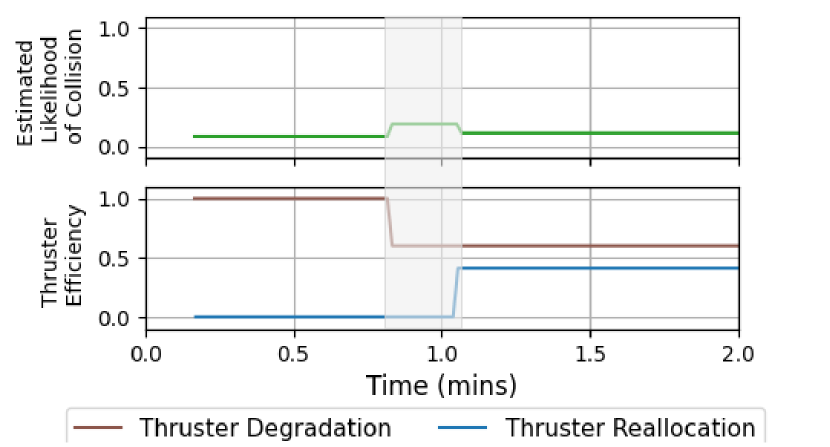
Figure 9: ReSonAte estimated likelihood of collision for the BlueROV2 example. As seen in gray shaded region, the likelihood of collision increases when thruster degradation occurs, then reduces after thruster control reallocation.

IV-B4 Results

Fig. 9 shows the ReSonAte estimated likelihood of collision. The efficiency of thruster 1 degrades to 60% at 45 seconds, and the estimated likelihood of collision increases to 0.25. Soon after, the contingency manager performs a thruster reallocation to improve the uuv’s stability, the likelihood of collision decreases to 0.15. We are currently validating the estimated likelihood across large simulation runs.

V Conclusion and Future Work

resonate captures design-time information about system hazard propagation, control strategies, and potential consequences using btd, then uses the information contained in these models to calculate risk at run-time. The frequency of threat events and the effectiveness of hazard control strategies influence the estimated risk and may be conditionally dependent on the state of the system and operating environment. A technique for measuring these conditional relationships in simulation using a custom sdl was demonstrated. resonate was then applied to an av example in the CARLA simulator to dynamically assess the risk of collision, and a strong correlation was found between the estimated likelihood of a collision and the observed collisions. Additionally, resonate’s risk calculations require minimal computational resources making it suitable for resource-constrained and real-time cps.

Future extensions and applications for resonate include: (1) dynamic estimation of event severity in addition to event likelihood, (2) inclusion of state uncertainty into risk calculations to produce confidence bounds on risk estimates, (3) forecasting future risk based on expected changes to system or environment, (4) use of estimated risk for higher-level decision making such as controller switching or enactment of contingency plans, and (5) continuous improvement of conditional probability estimates at run-time from operational data.

Acknowledgement: This work was supported by the DARPA Assured Autonomy project and Air Force Research Laboratory.

References

- [1] G. Schwalbe and M. Schels, “A survey on methods for the safety assurance of machine learning based systems,” in 10th European Congress on Embedded Real Time Software and Systems (ERTS 2020), 2020.
- [2] P. Koopman and M. Wagner, “Challenges in autonomous vehicle testing and validation,” SAE International Journal of Transportation Safety, vol. 4, no. 1, pp. 15–24, 2016.
- [3] FAA, “FAA System Safety Handbook,” December 2000.
- [4] P. Bishop and R. Bloomfield, “A methodology for safety case development,” in Safety and Reliability, vol. 20, no. 1. Taylor & Francis, 2000, pp. 34–42.
- [5] J. Rushby, “Runtime certification,” in International Workshop on Runtime Verification. Springer, 2008, pp. 21–35.
- [6] E. Denney, G. Pai, and I. Habli, “Dynamic safety cases for through-life safety assurance,” in 2015 IEEE/ACM 37th IEEE International Conference on Software Engineering, vol. 2. IEEE, 2015, pp. 587–590.
- [7] D. Schneider and M. Trapp, “Conditional safety certification of open adaptive systems,” ACM Transactions on Autonomous and Adaptive Systems (TAAS), vol. 8, no. 2, pp. 1–20, 2013.
- [8] A. Wardziński, “Safety assurance strategies for autonomous vehicles,” in International Conference on Computer Safety, Reliability, and Security. Springer, 2008, pp. 277–290.
- [9] Z. Kurd, T. Kelly, J. McDermid, R. Calinescu, and M. Kwiatkowska, “Establishing a framework for dynamic risk management in ‘intelligent’aero-engine control,” in International Conference on Computer Safety, Reliability, and Security. Springer, 2009, pp. 326–341.
- [10] F. L. Leite, D. Schneider, and R. Adler, “Dynamic risk management for cooperative autonomous medical cyber-physical systems,” in International Conference on Computer Safety, Reliability, and Security. Springer, 2018, pp. 126–138.
- [11] V. K. Sundar, S. Ramakrishna, Z. Rahiminasab, A. Easwaran, and A. Dubey, “Out-of-distribution detection in multi-label datasets using latent space of -vae,” arXiv preprint arXiv:2003.08740, 2020.
- [12] F. Cai and X. Koutsoukos, “Real-time out-of-distribution detection in learning-enabled cyber-physical systems,” in 2020 ACM/IEEE 11th International Conference on Cyber-Physical Systems (ICCPS). Los Alamitos, CA, USA: IEEE Computer Society, apr 2020, pp. 174–183. [Online]. Available: https://doi.ieeecomputersociety.org/10.1109/ICCPS48487.2020.00024
- [13] C. Katrakazas, M. Quddus, and W.-H. Chen, “A new integrated collision risk assessment methodology for autonomous vehicles,” Accident Analysis & Prevention, vol. 127, pp. 61–79, 2019.
- [14] A. Dosovitskiy, G. Ros, F. Codevilla, A. Lopez, and V. Koltun, “Carla: An open urban driving simulator,” arXiv:1711.03938, 2017.
- [15] N. Mahadevan, A. Dubey, and G. Karsai, “Application of software health management techniques,” in Proceedings of the 6th international symposium on software engineering for adaptive and self-managing systems, 2011, pp. 1–10.
- [16] A. N. Srivastava and J. Schumann, “The case for software health management,” in 2011 IEEE Fourth International Conference on Space Mission Challenges for Information Technology. IEEE, 2011, pp. 3–9.
- [17] G. Steinbauer and F. Wotawa, “Model-based reasoning for self-adaptive systems–theory and practice,” in Assurances for Self-Adaptive Systems. Springer, 2013, pp. 187–213.
- [18] T. Byun and S. Rayadurgam, “Manifold for machine learning assurance,” in Proceedings of the ACM/IEEE 42nd International Conference on Software Engineering: New Ideas and Emerging Results, 2020, pp. 97–100.
- [19] R. A. Clothier, B. P. Williams, and N. L. Fulton, “Structuring the safety case for unmanned aircraft system operations in non-segregated airspace,” Safety science, vol. 79, pp. 213–228, 2015.
- [20] B. P. Williams, R. Clothier, N. Fulton, S. Johnson, X. Lin, and K. Cox, “Building the safety case for uas operations in support of natural disaster response,” in 14th AIAA Aviation Technology, Integration, and Operations Conference, 2014, p. 2286.
- [21] E. Denney, G. Pai, and I. Whiteside, “Modeling the safety architecture of uas flight operations,” in Computer Safety, Reliability, and Security, S. Tonetta, E. Schoitsch, and F. Bitsch, Eds. Cham: Springer International Publishing, 2017, pp. 162–178.
- [22] ——, “The role of safety architectures in aviation safety cases,” Reliability Engineering & System Safety, vol. 191, p. 106502, 2019.
- [23] N. Khakzad, F. Khan, and P. Amyotte, “Dynamic risk analysis using bow-tie approach,” Reliability Engineering & System Safety, vol. 104, pp. 36–44, 2012.
- [24] C. Delvosalle, C. Fievez, A. Pipart, and B. Debray, “Aramis project: A comprehensive methodology for the identification of reference accident scenarios in process industries,” Journal of Hazardous Materials, vol. 130, no. 3, pp. 200–219, 2006.
- [25] R. Ferdous, F. Khan, R. Sadiq, P. Amyotte, and B. Veitch, “Handling data uncertainties in event tree analysis,” Process safety and environmental protection, vol. 87, no. 5, pp. 283–292, 2009.
- [26] A. Badreddine and N. Ben Amor, “A new approach to construct optimal bow tie diagrams for risk analysis,” in Trends in Applied Intelligent Systems, N. García-Pedrajas, F. Herrera, C. Fyfe, J. M. Benítez, and M. Ali, Eds. Berlin, Heidelberg: Springer Berlin Heidelberg, 2010, pp. 595–604.
- [27] A. Badreddine and N. B. Amor, “A bayesian approach to construct bow tie diagrams for risk evaluation,” Process Safety and Environmental Protection, vol. 91, no. 3, pp. 159–171, 2013.
- [28] M. Teimourikia, M. Fugini, and C. Raibulet, “Run-time security and safety management in adaptive smart work environments,” in 2017 IEEE 26th International Conference on Enabling Technologies: Infrastructure for Collaborative Enterprises (WETICE). IEEE, 2017, pp. 256–261.
- [29] Y. Zhang and X. Guan, “Selecting project risk preventive and protective strategies based on bow-tie analysis,” Journal of Management in Engineering, vol. 34, no. 3, p. 04018009, 2018.
- [30] M. Vileiniskis and R. Remenyte-Prescott, “Quantitative risk prognostics framework based on petri net and bow-tie models,” Reliability Engineering & System Safety, vol. 165, pp. 62–73, 2017.
- [31] A. Misra, “Senor-based diagnosis of dynamical systems,” Ph.D. dissertation, Vanderbilt University Ph. D. dissertation, 1994.
- [32] N. Mahadevan, A. Dubey, and G. Karsai, “Architecting health management into software component assemblies: Lessons learned from the arinc-653 component mode,” in 2012 IEEE 15th International Symposium on Object/Component/Service-Oriented Real-Time Distributed Computing. IEEE, 2012, pp. 79–86.
- [33] ISO, “ISO 26262:2018 Road vehicles - Functional safety,” December 2018.
- [34] O. Federal Aviation Administration, “Risk management handbook (faa-h-8083-2),” 2019. [Online]. Available: https://www.faa.gov/regulations_policies/handbooks_manuals/aviation/media/FAA-H-8083-2.pdf
- [35] T. P. Kelly, “Arguing safety: a systematic approach to managing safety cases,” Ph.D. dissertation, University of York York, UK, 1999.
- [36] C. Haddon-Cave, The Nimrod Review: an independent review into the broader issues surrounding the loss of the RAF Nimrod MR2 aircraft XV230 in Afghanistan in 2006, report. DERECHO INTERNACIONAL, 2009, vol. 1025.
- [37] N. G. Leveson, “The use of safety cases in certification and regulation,” 2011.
- [38] Y. Matsuno and S. Yamamoto, “Toward dynamic assurance cases.” in JCKBSE, 2012, pp. 154–160.
- [39] S. L. Zabell, “The rule of succession,” Erkenntnis, vol. 31, no. 2, pp. 283–321, 1989.
- [40] D. J. Fremont, T. Dreossi, S. Ghosh, X. Yue, A. L. Sangiovanni-Vincentelli, and S. A. Seshia, “Scenic: A language for scenario specification and scene generation,” in Proceedings of the 40th annual ACM SIGPLAN conference on Programming Language Design and Implementation (PLDI), June 2019.
- [41] O. foretellix, “Open m-sdl.” [Online]. Available: https://www.foretellix.com/open-language/
- [42] I. Dejanović, R. Vaderna, G. Milosavljević, and Ž. Vuković, “Textx: a python tool for domain-specific languages implementation,” Knowledge-Based Systems, vol. 115, pp. 1–4, 2017.
- [43] D. Karunakaran, S. Worrall, and E. Nebot, “Efficient statistical validation with edge cases to evaluate highly automated vehicles,” in 2020 IEEE 23rd International Conference on Intelligent Transportation Systems (ITSC). IEEE, 2020, pp. 1–8.
- [44] R. Calinescu, D. Weyns, S. Gerasimou, M. U. Iftikhar, I. Habli, and T. Kelly, “Engineering trustworthy self-adaptive software with dynamic assurance cases,” IEEE Transactions on Software Engineering, vol. 44, no. 11, pp. 1039–1069, 2017.
- [45] B. Robotics, “Bluerov2,” Datasheet, June, 2016.
- [46] D. Chen, B. Zhou, V. Koltun, and P. Krähenbühl, “Learning by cheating,” in Conference on Robot Learning. PMLR, 2020, pp. 66–75.
- [47] J. L. Pech-Pacheco, G. Cristóbal, J. Chamorro-Martinez, and J. Fernández-Valdivia, “Diatom autofocusing in brightfield microscopy: a comparative study,” in Proceedings 15th International Conference on Pattern Recognition. ICPR-2000, vol. 3. IEEE, 2000, pp. 314–317.
- [48] G. Shafer and V. Vovk, “A tutorial on conformal prediction,” Journal of Machine Learning Research, vol. 9, no. Mar, pp. 371–421, 2008.
- [49] V. Fedorova, A. Gammerman, I. Nouretdinov, and V. Vovk, “Plug-in martingales for testing exchangeability on-line,” arXiv preprint arXiv:1204.3251, 2012.
- [50] M. Quigley, K. Conley, B. P. Gerkey, J. Faust, T. Foote, J. Leibs, R. Wheeler, and A. Y. Ng, “Ros: an open-source robot operating system,” in ICRA Workshop on Open Source Software, 2009.
- [51] N. P. Koenig and A. Howard, “Design and use paradigms for gazebo, an open-source multi-robot simulator.” in Proceedings of 2004 IEEE/RSJ International Conference on Intelligent Robots and Systems. Citeseer, 2004.
- [52] M. M. M. Manhães, S. A. Scherer, M. Voss, L. R. Douat, and T. Rauschenbach, “UUV simulator: A gazebo-based package for underwater intervention and multi-robot simulation,” in OCEANS 2016 MTS/IEEE Monterey. IEEE, sep 2016. [Online]. Available: https://doi.org/10.1109%2Foceans.2016.7761080