Modulational instability and soliton generation in chiral Bose-Einstein condensates with zero-energy nonlinearity

Abstract

By means of analytical and numerical methods, we address the modulational instability (MI) in chiral condensates governed by the Gross-Pitaevskii equation including the current nonlinearity. The analysis shows that this nonlinearity partly suppresses off the MI driven by the cubic self-focusing, although the current nonlinearity is not represented in the system’s energy (although it modifies the momentum), hence it may be considered as zero-energy nonlinearity. Direct simulations demonstrate generation of trains of stochastically interacting chiral solitons by MI. In the ring-shaped setup, the MI creates a single traveling solitary wave. The sign of the current nonlinearity determines the direction of propagation of the emerging solitons.

I Introduction

Since the creation of the Bose-Einstein condensates (BECs) in 1995, they became versatile testbeds for the study of various physical phenomena in quantum states of matter Greiner et al. (2002); Bloch et al. (2008). One of striking properties of the condensates is their ability to emulate physics of charged particles under the action of magnetic fields Lin et al. (2011); Dalibard et al. (2011); Goldman et al. (2014) through engineering of synthetic gauge fields in such charge-neutral ultracold atomic gases.

Synthetic gauge fields can be introduced by means of rapid rotation of the condensate Matthews et al. (1999); Madison et al. (2000), optical coupling between internal states of atoms Juzeliūnas and Öhberg (2004); Juzeliūnas et al. (2006); Lin et al. (2009), laser-assisted tunneling Miyake et al. (2013); Aidelsburger et al. (2011), and Floquet engineering Parker et al. (2013). The nature of these gauge fields is essentially static, as parameters of field-inducing laser beams, including their intensity and phase gradients, cannot reproduce the time dependence of the Maxwell’s equations. Dynamical gauge fields, affected by nonlinear feedback from matter, to which the fields are coupled, are required to emulate a full time-dependent field theory. A number of schemes Banerjee et al. (2012); Zohar et al. (2013); Tagliacozzo et al. (2013); Greschner et al. (2014); Dong et al. (2014); Ballantine et al. (2017) have been proposed for creating dynamical gauge fields with ultra-cold atoms, including the ones which give rise to density-dependent gauge potentials and current nonlinearities Edmonds et al. (2013); Zheng et al. (2015). Following these proposals, such dynamical gauge fields have been experimentally realized recently Martinez et al. (2016); Clark et al. (2018); Görg et al. (2019).

The chiral condensates, interacting with gauge potentials, enrich physics of atomic and nonlinear systems, thus drawing much interest in experimental and theoretical studies. The presence of density-dependent gauge fields makes it possible to create anyonic structures Keilmann et al. (2011) and chiral solitons Edmonds et al. (2013); Aglietti et al. (1996), which opens new perspectives for quantum simulations. The chiral solitons move unidirectionally, the selected direction being determined by the current nonlinearity. The chiral solitons were considered for emulation of quantum time crystals (first envisaged by Wilczek in 2012 Wilczek (2012)) in circumferentially confined condensates with density-dependent gauge potentials Öhberg and Wright (2019, 2020, 2020). However, this proposal was disputed since, in the thermodynamic limit of the latter setting, the lowest-energy ground state is realized by a static soliton, hence a genuine time crystal is not feasible Syrwid et al. (2020a, b).

The chiral condensates have also been studied in the presence of persistent currents Edmonds et al. (2013) and collective excitations Edmonds, M. J. et al. (2015) in them. The evolution of the excitations is affected by the current nonlinearity, leading to irregular dynamics in a strongly nonlinear regime and related violation of the Kohn’s theorem. The current nonlinearities in chiral condensates, in addition to being responsible for nonintegrable collision dynamics in soliton pairs Dingwall et al. (2018), help to maintain rich dynamics in trapped condensates Saleh and Öhberg (2018).

In this paper, we study effects of the current nonlinearity on modulational instability (MI) (alias Benjamin-Feir instability Benjamin and Feir (1967)) of the chiral BEC. It is well known that MI is a natural precursor to the formation of solitonic coherent structures, as a result of the interplay between intrinsic self-interaction of the medium and diffraction or dispersion, and has been studied in diverse physical settings theoretically Benjamin and Feir (1967); Agrawal ; Mithun et al. (2020) and experimentally Everitt et al. (2017); Nguyen et al. (2017); Sanz et al. (2019). The MI strongly depends on the nature of two-body interactions in single-component condensates, where it occurs only in the case of self-attraction Theocharis et al. (2003); Salasnich et al. (2003). However, the intercomponent interactions make MI scenarios more diverse in multicomponent condensates. In particular, binary condensates with repulsive interactions are modulationally unstable under the condition of immiscibility Goldstein and Meystre (1997); Kasamatsu and Tsubota (2004, 2006). Static gauge fields which impose spin-orbit coupling make condensates still more vulnerable to MI Bhat et al. (2015); Mithun and Kasamatsu (2019). Further, helicoidal gauge potentials break the MI symmetry and thus strongly modify patterns of instability regions and gain in the underlying parameter space Li et al. (2019). In this connection, we investigate the effect of density-dependent gauge potentials on the MI and subsequent generation of solitons. Additionally, we consider the solitons in a circumferentially confined condensate in a moving reference frame. A specific peculiarity of the system is that the gauge potential is represented in the respective Gross-Pitaevskii (GP) equation by a current nonlinearity, which, however, is not represented by any term in the system’s energy. Thus, this term may be identified as an example of zero-energy nonlinearity. To the best of our knowledge, effects of such terms on the MI were not studied before.

The subsequent material is organized as follows. Sec. II introduces the model and the corresponding GP equation including the density-dependent gauge potential. In Sec. III the dispersion relation produced by the linear MI analysis is derived and discussed. Sec. IV reports results of numerical simulations of the system under the consideration. The work is concluded by Sec. V.

II The model

We consider a condensate of two-level atoms with the Rabi coupling imposed by an incident laser beam, as described by the following mean-field Hamiltonian Goldman et al. (2014); Edmonds et al. (2013):

$$\begin{split}\mathcal{\hat{H}}&=\bigg{(}\frac{\mathbf{\hat{p}}^{2}}{2m}+V(\mathbf{r})\bigg{)}\mathbf{\check{I}}+\\ &\begin{pmatrix}g_{11}\lvert\Psi_{1}\rvert^{2}+g_{12}\lvert\Psi_{2}\rvert^{2}&\frac{\hbar\Omega_{r}}{2}e^{-i\phi(\mathbf{r})}\\ \frac{\hbar\Omega_{r}}{2}e^{i\phi(\mathbf{r})}&g_{22}\lvert\Psi_{2}\rvert^{2}+g_{12}\lvert\Psi_{1}\rvert^{2}\end{pmatrix}\end{split}$$ (1)

where $\mathbf{\hat{p}}$ is the momentum operator, $V(\mathbf{r})$ is the trapping potential, $\mathbf{\check{I}}$ is the unity matrix, $\Omega_{r}$ is the Rabi-coupling strength, $\phi(\mathbf{r})$ is a spatially varying phase of the coupling beam, and $g_{\mu\nu}=\left(2\pi\hbar^{2}/m\right)a_{\mu\nu}$ are the mean-field interaction strengths, proportional to respective scattering lengths, $a_{\mu\nu}$, of collisions between atoms in internal states $\mu$ and $\nu$ ($\mu,\nu=1,2$). At the mean-field level, atomic collisions result in effective density-dependent detunings of the atomic states. In the case of dilute condensates, when the Rabi-coupling energy dominates over the collisional detunings, the perturbative approach leads to the following density-dependent gauge potential Edmonds et al. (2013):

$$\mathbf{A}=\mathbf{A}_{0}+n\leavevmode\nobreak\ \frac{g_{11}-g_{22}}{8\Omega_{r}}\nabla\phi(\mathbf{r})$$ (2)

where $\mathbf{A}_{0}=-\left(\hbar/2\right)\nabla\phi(\mathbf{r})$ represents the single-particle vector potential, and $n$ is the density of the condensate. By projecting the coupled two-level atom onto a single dressed state, one arrives at the following mean-field GP equation governing the dynamics of chiral condensates: Aglietti et al. (1996); Edmonds et al. (2013); Edmonds, M. J. et al. (2015); Saleh and Öhberg (2018):

$$i\hbar\frac{\partial\Psi}{\partial t}=\bigg{[}\frac{(\mathbf{\hat{p}}-\mathbf{A)^{2}}}{2m}+W(\mathbf{r})+V(\mathbf{r})+\mathfrak{g}|\Psi|^{2}+\mathbf{a_{1}}\cdot\mathbf{J}(\Psi,\Psi^{\ast})\bigg{]}\Psi$$ (3)

where $\Psi$ is the wave function of the dressed state. Further, $W(\mathbf{r})=\lvert A_{0}\rvert^{2}/\left(2m\right)$, together with the trapping potential, $V(\mathbf{r})$, defines the scalar potential, $\mathbf{a_{1}}=\left(g_{11}-g_{22}\right)/\left(8\Omega_{r}\right)\nabla\phi(\mathbf{r})$ is the strength of the density-dependent vectorial gauge potential, and $\mathfrak{g}=(1/4)(g_{11}+g_{22}+2g_{12})$ determines the effective interaction in the dressed-state picture. The unconventional nonlinearity in the chiral condensates manifests itself in Eq. (3) through the current,

$$\mathbf{J}(\Psi,\Psi^{\ast})=\frac{\hbar}{2im}\bigg{[}\Psi\bigg{(}\nabla+\frac{i}{\hbar}\mathbf{A}\bigg{)}\Psi^{\ast}-\Psi^{\ast}\bigg{(}\nabla-\frac{i}{\hbar}\mathbf{A}\bigg{)}\Psi\bigg{]}$$ (4)

Defining $\phi(x)=k_{l}x$, where $k_{l}$ is the wavenumber of the incident laser beam, following the usual procedure of the dimensional reduction Dingwall et al. (2018), and applying the nonlinear phase transformation,

$$\Psi(x,t)=\psi(x,t)\leavevmode\nobreak\ \exp\left[-i\frac{\phi(x)}{2}+i\frac{a_{1}}{\hbar}\int_{-\infty}^{x}dx^{\prime}n(x^{\prime},t)-i\frac{Wt}{\hbar}\right]\text{,}$$ (5)

Eq. (3) is cast in the form of the following one-dimensional (1D) GP equation:

$$i\hbar\frac{\partial}{\partial t}\psi=\bigg{(}-\frac{\hbar^{2}}{2m}\frac{\partial^{2}}{\partial x^{2}}+V(x)+g|\psi|^{2}-2\alpha J(x)\bigg{)}\psi$$ (6)

where $V(x)=\left(1/2\right)m\omega_{x}^{2}x^{2}$ is the 1D trapping potential with axial trapping frequency $\omega_{x}$, $g\equiv\mathfrak{g}/2\pi a_{\perp}^{2}$ is the usual coefficient of the cubic nonlinearity, and $a_{\perp}=\sqrt{\hbar/\left(m\omega_{\perp}\right)}$ is the harmonic-oscillator length of the transverse confining potential. In Eq. (6) $\alpha=\left(2\pi a_{\perp}^{2}\right)^{-1}\left[k_{l}(g_{11}-g_{22})/\left(8\Omega_{r}\right)\right]$ is the strength of the unconventional current nonlinearity, which involves the current density, $J(x)=\left(i\hbar/2m\right)(\psi\partial_{x}\psi^{\ast}-\psi^{\ast}\partial_{x}\psi)$. Spatiotemporal rescaling,

$$t^{\prime}=\omega_{\perp}t,\leavevmode\nobreak\ \leavevmode\nobreak\ x^{\prime}=\frac{x}{a_{\perp}},\leavevmode\nobreak\ \psi^{\prime}=\sqrt{a_{\perp}}\psi,$$ (7)

casts Eq. (6) in the normalized form:

$$i\partial_{t}\psi=\bigg{(}-\frac{1}{2}\partial_{xx}+\sigma|\psi|^{2}-2\rho J(x)\bigg{)}\psi.$$ (8)

In Eq. (8), the current density is now defined as

$$J(x)=\left(i/2\right)(\psi\partial_{x}\psi^{\ast}-\psi^{\ast}\partial_{x}\psi),$$ (9)

and the axial potential, which is $V(x)$ in Eq. (6), is dropped, as the following analysis deals with the dynamics in free space. The generalized GP equation (8), with scaled interaction parameters $\sigma=\left(a_{11}+a_{22}+2a_{12}\right)/\left(2a_{\perp}\right)$ and $\rho=\left(\hbar k_{l}/4m\Omega_{r}\right)(a_{11}-a_{22})/a_{\perp}^{2}$, is used below for the consideration of MI and formation of chiral solitons. Note that solutions of Eq. (8) with $\sigma<0$ for quiescent solitons, with an arbitrary real chemical potential, $\mu<0$, are precisely the same as in the case of $\rho=0$:

$$\psi_{\mathrm{sol}}=e^{-i\mu t}\sqrt{2\mu/\sigma}\mathrm{sech}\left(\sqrt{-2\mu}x\right).$$ (10)

Equations (8) and (9) conserve the integral norm (proportional to the total number of particles), $N=\int_{-\infty}^{+\infty}dx|\psi|^{2}$, energy,

$$E=-\frac{1}{2}\int_{-\infty}^{+\infty}dx\left(\left|\frac{\partial\psi}{\partial x}\right|^{2}+\sigma|\psi|^{4}\right),$$ (11)

and momentum,

$$P=-\int_{-\infty}^{+\infty}dx\left(J(x)+\rho|\psi|^{4}\right)$$ (12)

Dingwall et al. (2018); Jackiw (1997). Unlike the underlying chiral GP equation (3), the transformed equation (8) cannot be written in the Lagrangian form. It cannot be written in the Hamiltonian form either, but, nevertheless, energy $E$, defined by Eq. (11), is its dynamical invariant. It is worthy to note that the energy conservation holds in spite of the fact $E$ does not include any term $\sim\rho$ (in fact, $E$ is the same as for the usual non-chiral GP equation), i.e., the current term may be identified as zero-energy nonlinearity [although it affects expression (12) for the conserved momentum]. The conservation of $E$ can be readily verified by the straightforward calculation of $dE/dt$, substituting $\partial\psi/\partial t$ and $\partial\psi^{\ast}/\partial t$ in the integrand by what is produced by Eq. (8). As a result, the terms $\sim\rho$ amount to expressions in the form of full $x$-derivatives, hence their contribution to the integral expression for $dE/dt$ identically vanishes for all localized states, the result being $dE/dt=0$.

Qualitatively, a term in conservative equations which does not affect the energy may be compared to the Lorentz force acting on a charged particle in magnetic field, or the Coriolis force for a body moving on a rotating sphere. However, such an analogy is not an accurate one, because the Lorentz and Coriolis forces, although they are not represented in the particle’s Hamiltonian, appear in the Lagrangian, while, as mentioned above, the term $\sim\rho$ in Eq. (8) cannot be derived from a Lagrangian. In terms of models governed by GP-like equations, somewhat similar effects are produced by the stimulated Raman scattering (SRS) in fiber optics Gordon (1986) and its pseudo-SRS counterpart in the system of interacting high- and low-frequency waves (the Zakharov system) Gromov and Malomed (2013), as well as by the nonlinear Landau damping in plasmas Ichikawa (1979). However, in those cases the non-Lagrangian terms conserve only the norm of the wave fields, while causing the dissipation of the energy and momentum (in particular, self-decelaration of solitons Gordon (1986)), therefore the latter analogy is not accurate either.

On the other hand, the current nonlinearity in Eq. (8) makes the total momentum, as given by Eq. (12), different from the standard expression for the non-chiral GP equation. In this connection, it is also relevant to mention that, unlike the usual GP equation, Eq. (8) is not invariant with respect to the Galilean transform: the substitution of

$$\tilde{x}=x-ut,\leavevmode\nobreak\ \psi=\exp\left(iux-iu^{2}t/2\right)\tilde{\psi}\left(\tilde{x},t\right),$$ (13)

transforms Eq. (8) not into the equation of the same form for wave function $\tilde{\psi}\left(\tilde{x},t\right)$, written in the reference frame moving with arbitrary velocity $u$, but into one with $\sigma$ replaced by

$$\tilde{\sigma}=\sigma-2\rho u.$$ (14)

Note that taking $\rho u>\sigma/2$ replaces $\sigma>0$ (self-repulsion) by $\tilde{\sigma}<0$ (self-attraction), and vice versa, taking $\rho u<\sigma/2$, in the case of $\sigma<0$.

According to Eqs. (13) and (14), the solution of Eq. (8) for a soliton moving with velocity $u$ is obtained from the quiescent one (10) Dingwall et al. (2018):

$$\begin{split}\psi_{\mathrm{sol}}&=\exp\left(iux-i\left(\mu+u^{2}/2\right)t\right)\sqrt{2\mu/\left(\sigma-2\rho u\right)}\\ &\times\mathrm{sech}\left(\sqrt{-2\mu}\left(x-ut\right)\right).\end{split}$$ (15)

Obviously, this solution exists for $\mu<0$ and $2\rho u-\sigma>0$. In the framework of the non-integrable GP equation (8), collisions between solitons moving at different velocities were studied in Ref. Dingwall et al. (2018), revealing various inelastic outcomes of the collisions.

Lastly, as concerns dissipative effects, parameters of the loss, chiefly induced by collisions of atoms from the condensate with ones belonging to the thermal component of the gas, were calculated, in particular, in Ref. Choi et al. (1998). Estimates based on these values easily demonstrate that the dissipation is not an essential factor for experimentally relevant times.

III The linear-stability analysis (LSA)

We examine the MI via linear instability analysis (LSA) of the spatially uniform (alias continuous-wave, CW) state of the chiral condensate in the absence of the external potential, $V(x)=0$. The respective linearized Bogoliubov-de Gennes equations for small perturbations about the CW wave function were derived in Refs. Edmonds, M. J. et al. (2015); Dingwall et al. (2018), though the MI spectrum has not been derived, and is addressed here. The usual CW solution to Eq. (8) is

$$\psi(x,t)=\sqrt{n}\exp\left(iKx-i\mu_{\mathrm{CW}}t\right),$$ (16)

with arbitrary density, $n=|\psi|^{2}$, real wavenumber $K$, and chemical potential $\mu_{\mathrm{CW}}={\sigma n-2\rho K}$. It is more convenient to develop the MI analysis in the reference frame moving at velocity $u=K$, applying the Galilean transformation provided by Eq. (13). It removes term $Kx$ from the CW phase, replacing $\sigma$ by

$$\tilde{\sigma}=\sigma-2\rho K,$$ (17)

as per Eq. (14).

We perturb the CW state (16), replacing it by (in the moving reference frame, if $K\neq 0$)

$$\psi=(\sqrt{n}+\delta\psi\left(x,t\right))\exp\left(-i\mu_{\mathrm{CW}}t\right),$$ (18)

which results in the following linearized equation for the small perturbation, $\delta\psi(x,t)$:

$$i\partial_{t}(\delta\psi)=-\frac{1}{2}\partial_{xx}^{2}(\delta\psi)+n\tilde{\sigma}(\delta\psi+\delta\psi^{\ast})+in\rho\left(\partial_{x}\delta\psi-\partial_{x}\delta\psi^{\ast}\right)$$ (19)

where $\ast$ stands for the complex conjugate, and $x$ is written instead of $\tilde{x}$, to simplify the notation, if the moving reference frame is used. We look for eigenmodes of the perturbations in the usual plane-wave form, $\delta\psi=a\cos(kx-\Omega t)+ib\sin(kx-\Omega t)$, with real wavenumber $k$ and complex eigenfrequency, $\Omega$, assuming that the actual system’s size is much greater than the healing length which determines a characteristic MI length scale. The substitution of this in Eqs. (19) and (9) results in the following dispersion equation:

$$\Omega^{2}+2n\rho k\leavevmode\nobreak\ \Omega-n\tilde{\sigma}k^{2}-\frac{k^{4}}{4}=0,$$ (20)

which yields two branches of the $\Omega(k)$ dependence:

$$\Omega_{\pm}=-n\rho k\pm\sqrt{\frac{k^{4}}{4}+k^{2}n(n\rho^{2}+\tilde{\sigma})}$$ (21)

Equation (21) is the Bogoliubov dispersion relation Bogolyubov (1947) for the propagation of small perturbations on top of the CW background. The expression on the right-hand side of Eq. (21) may be positive, negative or complex, depending on the signs and magnitudes of the interaction parameters. The CW solutions are stable if $\Omega_{\pm}(k)$ are real for all real $k$; otherwise, the instability gain is defined as $\xi\equiv\lvert\text{Im}(\Omega_{\pm})\rvert$. For $\rho=0$ (no current nonlinearity), the above consideration reproduces the well-known results for BEC with the cubic self-attraction ($\sigma<0$), yielding the MI in the wavenumber band $0<k<2\sqrt{n\lvert\sigma\rvert}$, with the maximum MI gain, $\xi_{\max}=n\lvert\sigma\rvert$, attained at $k_{\max}=\sqrt{2n\lvert\sigma\rvert}$ Benjamin and Feir (1967); Theocharis et al. (2003).

The effect of the current nonlinearity, quantified by coefficient $\rho$, on the MI can be understood in the framework of Eq. (21). It is evident that the MI gain is essentially the same for both signs of the current nonlinearity, $\rho$. Further, such chiral condensates may be modulationally unstable only for the attractive sign of the two-body interactions, i.e., $\tilde{\sigma}<0$. The current-nonlinearity’s strength, $\rho$, controls the MI region and gain for a fixed value of $\tilde{\sigma}$, as shown in Fig. 1. It is found from Eq. (21) that the system is subject to the MI in the wavenumber range of $0<k<2\sqrt{n\lvert\tilde{\sigma}\rvert-n^{2}\rho^{2}}$, provided that

$$\rho<\sqrt{\lvert\tilde{\sigma}\rvert/n}.$$ (22)

For $\rho\geq\sqrt{\lvert\tilde{\sigma}\rvert/n}$, the CW state is modulationally stable even for attractive two-body interactions, thereby revealing the stabilizing effect of the current nonlinearity in the chiral condensates. Further, substituting definition (17) in Eq. (22), the parameter region in which the MI takes place for $\rho K\neq 0$ amounts to the following interval of the current-nonlinearity’s strength:

$$K-\sqrt{K^{2}-\sigma n}<n\rho<K+\sqrt{K^{2}-\sigma n},$$ (23)

which exists provided that the cubic-nonlinearity coefficient satisfies condition

$$\sigma n<K^{2}.$$ (24)

In particular, this condition holds for all $\sigma<0$, while $K\neq 0$ may impose the MI even in the case when the cubic term in Eq. (8) is self-defocusing, with $\sigma>0$.

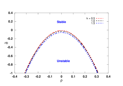
Figure 1: (Color online) The MI stability diagram, determined by Eq. (21) for $n=10$ and different values of $k$ in the $\left(\tilde{\sigma},\rho\right)$ plane: as it follows Eq. (21), the CW state is modulationally stable for $\rho^{2}\geq\left(k^{2}-4\tilde{\sigma}n\right)/\left(4n^{2}\right)$. Note the symmetry of the curves about $\rho=0$.

In combination with the Feshbach-resonance techniques Blatt et al. (2011); Inouye et al. (1998); Cornish et al. (2000), which makes it possible to adjust the value of $\sigma$, the chiral-interaction strength, $\rho,$ can be used to tune the MI gain, including suppression of the instability. This possibility can be adequately described in terms of the change of the maximum MI gain $\xi_{\max}$ at $k=k_{\max}$, following the variation of $\rho$. It follows from Eq. (21) that, for $\rho<\sqrt{\lvert\tilde{\sigma}\rvert/n}$, the largest MI gain,

$$\xi_{\max}=n(|\tilde{\sigma}|-n\rho^{2})$$ (25)

is attained at

$$k_{\max}=\pm\sqrt{2n(|\tilde{\sigma}|-n\rho^{2})}.$$ (26)

It is seen from Eqs. (25) and (26) that both $\xi_{\max}$ and $k_{\max}$ decrease monotonically with the increase of $\rho$, up to $\rho=\sqrt{\lvert\tilde{\sigma}\rvert/n}$, as shown in Fig. 2. The value $\xi_{\max}$ vanishes at $\rho^{2}=|\tilde{\sigma}|/n$, which is the above-mentioned MI boundary, given by Eq. (22).

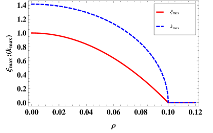
Figure 2: (Color online) Variation of $\xi_{\max}$ and $k_{\max}$ as a function of the current-nonlinearity’s strength, $\rho$, for $n=10\leavevmode\nobreak\ \text{and}\leavevmode\nobreak\ \tilde{\sigma}=-0.1$, as per Eqs. (25) and Eq. (26). The MI boundary, $\rho=0.1$, is given by Eq. (22).

A plot of the variation of $k_{\max}$ with the change of the strength of the nonlinearity coefficients, $\rho$ and $\tilde{\sigma}$, is presented, in the form of a heatmap, in Fig. 3, as per Eq. (26). This plot also shows that the addition of the current nonlinearity results in the stabilization of the condensate against the modulational perturbations.

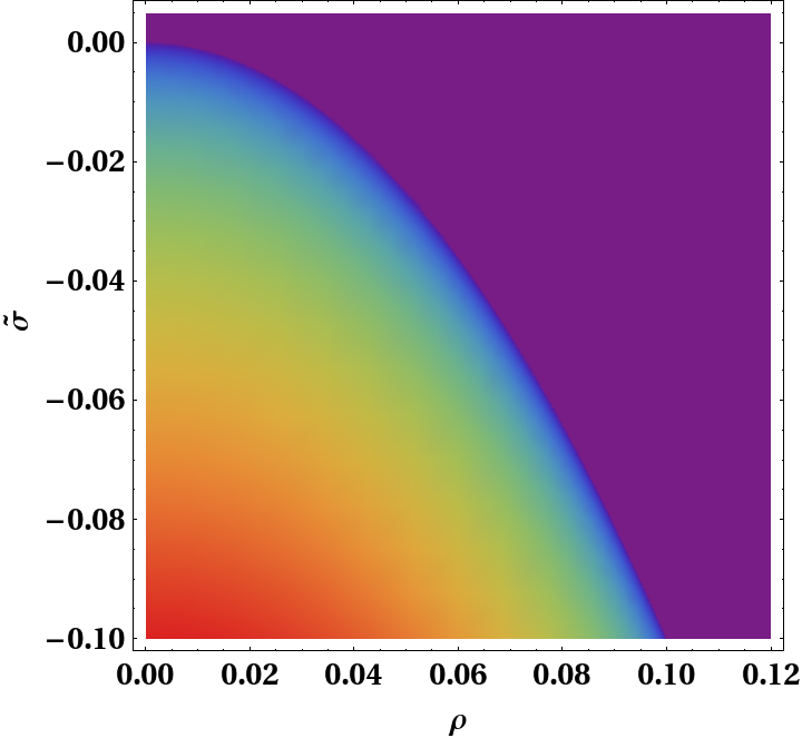
Figure 3: (Color online) The perturbation wavenumber, $k_{\max}$, at which the MI gain attains its maximum, as a function of the strengths of the two-body (cubic) attraction, $\tilde{\sigma}$, and the current nonlinearity, $\rho$, for $n=10$.

Next we study the variation of MI gain with respect to the strength of the two-body attraction, $\tilde{\sigma}$, at a fixed value of the current-nonlinearity’s strength, $\rho$. As mentioned above, the system is modulationally unstable if and only if the two-body interaction is attractive and condition (22) holds. The maximum MI gain, $\xi_{\max}$, as given by Eq. (25), is plotted in Fig. 4. Accordingly, the dependence of $\xi_{\max}$ on $\tilde{\sigma}$ is linear, with the slope determined by the CW density $n$.

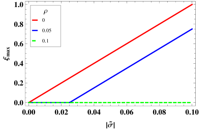
Figure 4: (Color online) Variation of $\xi_{\max}$ as a function of the strength of the two-body interaction, $\lvert\tilde{\sigma}\rvert$, for three fixed values of the current-nonlinearity’s strength, $\rho$ and $n=10$.

IV Numerical results

Proceeding to the numerical analysis, we employed a sixth-order Runge-Kutta scheme for simulations of the GP equation (8), cf. Refs. Sarafyan (1972); Edwards and Burnett (1995). The kinetic-energy term was dealt with by dint of the fast Fourier transform, while the spatial derivative in the current-nonlinearity part we approximated by the fourth-order central-difference formula. In the simulations, we fixed the timestep, $\Delta t=0.0001$, the domain size, $L=100$, and the spatial mesh size, $\Delta x=L/N$ with $N=2048$, unless mentioned otherwise.

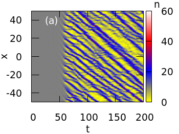
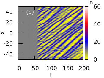
Figure 5: (Color online) The evolution of the condensate density due to the development of the MI for the cubic-attraction strength $\sigma=-0.1$ with (a) $\rho=0.08$, and (b) $\rho=-0.08$.

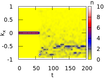
Figure 6: (Color online) The evolution of the condensate density in the $k$-space for the cubic-attraction and current-nonlinearity’s strengths $\sigma=-0.1$ and $\rho=0.08$. The circle at $t=62$ indicates the wavenumber, $k_{\max}\approx 0.81$, at which the MI-induced mode features the maximum of $n(k_{x})$, see the text.

The initial condition was taken as the CW background with uniform density, $n=10$, and $K=0$ [see Eq. (16)], seeded by weak random perturbations. It is clearly seen from Fig. 2 that the system is modulationally unstable for $\sigma=-0.1$, provided that $\rho<0.1$. Figure 5(a) shows the spatiotemporal evolution of the initially perturbed CW density for parameters $\sigma=-0.1,\leavevmode\nobreak\ \rho=0.08$. It shows generation of a train of chiral solitons at $t\geq 50$, propagating in the negative $x$-direction. The unidirectional propagation is a signature of the chiral solitons, see Eq. (15). Further, solitons belonging to the train collide inelastically due to the nonintegrability of the model Dingwall et al. (2018). The direction of motion of the solitons is determined by the sign of $\rho$, while the occurrence of the MI is independent of this sign, as shown in the previous section. To confirm this expectation, in Fig. 5(b) we set $\rho=-0.08$ for the same $\sigma=-0.1$. This simulation gives rise to a soliton train, with the same structure, but propagating in the positive $x$-direction. The choice of the propagation direction by the generated solitons can be understood from the $k$-space density, $n(k_{x})$, shown in Fig. 6, where modes with $k_{x}<0$ are chiefly excited.

The wavenumber corresponding to the maximum of $n\left(k_{x}\right)$ in the spontaneously excited mode is $k_{x}\approx 0.81$. Note that it is close to $k_{\max}=0.84$ predicted by the LSA. Further, values $k_{\max}=0.84$ and $\xi_{\max}=0.36$ correspond, severally, to the fastest growing mode with wavelength $\lambda_{\max}\equiv 2\pi/k_{\max}\approx 7.4$ and growth time scale $\tau=2\pi/\xi_{\max}\approx 17$. In turn, $\lambda_{\max}$ determines the number of solitons in the train observed in Fig. 5, as $\mathrm{n}_{\mathrm{sol}}\simeq L/\lambda\approx 14$, where $L=100$ is the above-mentioned size of the simulation domain.

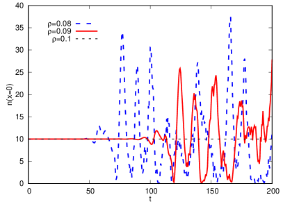
Figure 7: (Color online) The evolution of MI at different values of the current-nonlinearity’s strengths, $\rho$, and fixed self-attraction coefficient, $\sigma=-0.1$, is displayed in terms of the midpoint density, $n(x=0)$. For $\sigma<0$, the condensate is modulationally stable at $\rho\geq\sqrt{|\sigma|/n}$, see Eq. (22).

We extend the numerical analysis by varying $\rho$ at fixed $\sigma$. Figure 7 shows the temporal evolution of the midpoint density, $n(x=0)$, for $\rho=(0.1,0.09,0.08)$. The MI condition (22), predicted by LSA, is exactly confirmed by the figure. Further, it is seen that, as $\rho$ increases towards value $\sqrt{|\sigma|/n}$, above which the MI is suppressed, instability-growth time increases, due to the decrease in the MI gain, in agreement with Fig. 2. Numerical data produced by these simulations are summarized in Table 1. It is clearly seen that the findings agree with the predictions of the LSA analysis.

Table 1: The summary of the MI characteristics produced by the LSA and numerical simulations for the fixed cubic-attraction coefficient, $\sigma=0.1$, fixed CW density, $n=10$, and different values of the current-nonlinearity’s strength, $\rho$. Wavenumber $k_{\max}$ and the respective wavelength, $\lambda=2\pi/k_{\max}$, corresponding to the largest MI gain, $\xi_{\max}$, are given by Eq. (26). The MI growth time, $\tau=1/\xi_{\max}$, is determined by Eq. (25). The number of solitons in the MI-generated train is accurately approximated by estimate $\mathrm{n}_{\mathrm{sol}}\simeq L/\lambda$, see the text.

$\sigma$	$\rho$	$k_{max}$	$\lambda$	$\tau$	number of solitons
$-0.1$	$0.05$	$1.22$	$5.13$	$8.37$	$\sim 19$
	$0.08$	$0.84$	$7.40$	$17.45$	$\sim 14$
	$0.09$	$0.61$	$10.19$	$33.06$	$\sim 10$
	$0.1$	$0$	$\infty$	$\infty$	$\leavevmode\nobreak\ \leavevmode\nobreak\ \leavevmode\nobreak\ \leavevmode\nobreak\ 0$

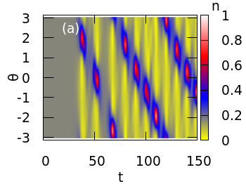
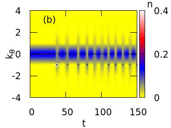
Figure 8: (Color online) Numerically simulated evolution of MI in a circumferentially confined condensate with $\tilde{g}=-3.6$, $\mathit{a}=\frac{\pi}{4}$ and $\int_{0}^{2\pi}d\theta|\varphi(\theta,\tau)|^{2}=1$. The white circle represents the wave vector corresponding to the initially excited mode.

Lastly, we address the 1D setting corresponding to the ring geometry with radius $R$ and periodic boundary conditions, the accordingly rescaled form of Eqs. (8) and (9) being

$$i\frac{\partial\varphi(\theta,\tau)}{\partial\tau}=\bigg{(}-\frac{1}{2}\frac{\partial^{2}}{\partial\theta^{2}}+\tilde{g}|\varphi|^{2}-2\mathit{a}J(\theta)\bigg{)}\varphi(\theta,\tau),$$ (27)

with $J(\theta)=(i/2)\text{Im}(\varphi\partial_{\theta}\varphi^{\ast}-\varphi^{\ast}\partial_{\theta}\varphi)$ and wave function $\varphi$ subject to the normalization condition $\int_{0}^{2\pi}d\theta|\varphi(\theta,\tau)|^{2}=1$, where $\theta$ is the angular coordinate on the ring. The accordingly scaled parameters are $\tilde{g}=\left(g-2\alpha u\right)\left(mR^{2}/\hbar^{2}\right)$ and $\mathit{a}=\alpha R/\hbar$, with $\alpha\equiv q(g_{11}-g_{22})/\left(8\Omega_{r}R\right)$ determined by integer winding number $q$ of the laser beam used to induce the circumferential gauge potentials. In this case, the CW state (18), including term $K\theta$ in the phase, can be constructed too, with integer values of $K$ allowed by the circular boundary condition.

As typical parameter values, we take $\mathit{a}=\pi/4$, $u=-1/4$ and $g=-4$, the respective cubic-term coefficient in Eq. (27) being $\tilde{g}=-3.6$. Note that this value satisfies condition $g<-\pi$, which is necessary to the transition from the uniform state in the ring to a soliton-like pattern Kanamoto et al. (2003). For this case, Fig. 8 shows the nonlinear evolution of the weak perturbations, initiated by the MI, that ultimately coalesce into a single chiral soliton, which performs circular motion on the ring. Note that the system does not converge to an equilibrium state that would be appropriate for the realization of the quantum time crystal. In addition to the spatial distribution of the density, displayed in 8(a), panel 8(b) shows that the wavenumber corresponding to the initially excited mode is $|k_{\theta}|=1$. It matches well to the analytical estimate given by the Eq. (26), even if it was derived for the infinite system, rather than for the circumference. As mentioned above, owing to the ring geometry of the condensate, only integer values are allowed for wavenumbers $k$. Consequently, the condensate undergoes oscillation in the $k-$space, as observed in Fig. 8(b).

V Conclusion

We have studied the MI (modulational instability) of the chiral condensate by means of LSA (linear stability analysis) and direct simulations. The chirality is introduced by the action of the current nonlinearity. A peculiar property of this nonlinearity is its zero-energy character, as, being accounted for by term $\sim\rho$ in the underlying GP equation (8), it is not represented in the respective energy, given by Eq. (11). Nevertheless, the current nonlinearity strongly affects the MI, tending to suppress it. Direct simulations demonstrate that, as long as the MI is present, it generates a train of stochastically interacting chiral solitons in the extended system, or a single soliton in the ring-shaped one. The MI gain does not depend on the sign of the current nonlinearity, although the sign determines the direction of the motion of the generated solitons.

An interesting extension of the work may be the consideration of GP (Gross-Pitaevskii) equations including the current nonlinearity in a combination with nonlinear terms that give rise to the onset of the critical collapse. In the 1D setting, the collapse is induced by the self-focusing quintic term, which may represent attractive three-body interactions in the atomic condensate Abdullaev et al. (2001); Abdullaev and Salerno (2005). A crude estimate of the virial type Fibich (2015) suggests that the current nonlinearity, although it is not represented in the system’s energy, may compete on a par with the quintic self-attraction, hence it may essentially affect the collapse dynamics. Further, the same current term can be added, as a quasi-1D one, to the two-dimensional (2D) GP equation, with the usual cubic self-attraction, which drives the development of the critical collapse in 2D Fibich (2015). An estimate suggests that, in the 2D setup, the current nonlinearity will be the strongest term in the collapsing regime, hence its effect may be crucially important.

VI Acknowledgements

We thank Dr. T. Mithun for useful discussions. The work of B.A.M. was supported, in part, by the Israel Science Foundation through grant No. 1286/17.

References

- Greiner et al. (2002) M. Greiner, O. Mandel, T. Esslinger, T. W. Hänsch, and I. Bloch, “Quantum phase transition from a superfluid to a mott insulator in a gas of ultracold atoms,” Nature 415, 39 (2002).
- Bloch et al. (2008) I. Bloch, J. Dalibard, and W. Zwerger, “Many-body physics with ultracold gases,” Rev. Mod. Phys. 80, 885 (2008).
- Lin et al. (2011) Y.-J. Lin, K. Jiménez-García, and I. B. Spielman, “Spin–orbit-coupled bose–einstein condensates,” Nature 471, 83 (2011).
- Dalibard et al. (2011) J. Dalibard, F. Gerbier, G. Juzeliūnas, and P. Öhberg, “Colloquium: Artificial gauge potentials for neutral atoms,” Rev. Mod. Phys. 83, 1523 (2011).
- Goldman et al. (2014) N. Goldman, G. Juzeliūnas, P. Öhberg, and I. B. Spielman, “Light-induced gauge fields for ultracold atoms,” Reports on Progress in Physics 77, 126401 (2014).
- Matthews et al. (1999) M. R. Matthews, B. P. Anderson, P. C. Haljan, D. S. Hall, C. E. Wieman, and E. A. Cornell, “Vortices in a bose-einstein condensate,” Phys. Rev. Lett. 83, 2498 (1999).
- Madison et al. (2000) K. W. Madison, F. Chevy, W. Wohlleben, and J. Dalibard, “Vortex formation in a stirred bose-einstein condensate,” Phys. Rev. Lett. 84, 806 (2000).
- Juzeliūnas and Öhberg (2004) G. Juzeliūnas and P. Öhberg, “Slow light in degenerate fermi gases,” Phys. Rev. Lett. 93, 033602 (2004).
- Juzeliūnas et al. (2006) G. Juzeliūnas, J. Ruseckas, P. Öhberg, and M. Fleischhauer, “Light-induced effective magnetic fields for ultracold atoms in planar geometries,” Phys. Rev. A 73, 025602 (2006).
- Lin et al. (2009) Y.-J. Lin, R. L. Compton, K. Jiménez-García, J. V. Porto, and I. B. Spielman, “Synthetic magnetic fields for ultracold neutral atoms,” Nature 462, 628 (2009).
- Miyake et al. (2013) H. Miyake, G. A. Siviloglou, C. J. Kennedy, W. C. Burton, and W. Ketterle, “Realizing the harper hamiltonian with laser-assisted tunneling in optical lattices,” Phys. Rev. Lett. 111, 185302 (2013).
- Aidelsburger et al. (2011) M. Aidelsburger, M. Atala, S. Nascimbène, S. Trotzky, Y.-A. Chen, and I. Bloch, “Experimental realization of strong effective magnetic fields in an optical lattice,” Phys. Rev. Lett. 107, 255301 (2011).
- Parker et al. (2013) C. V. Parker, L.-C. Ha, and C. Chin, “Direct observation of effective ferromagnetic domains of cold atoms in a shaken optical lattice,” Nature Physics 9, 769 (2013).
- Banerjee et al. (2012) D. Banerjee, M. Dalmonte, M. Müller, E. Rico, P. Stebler, U.-J. Wiese, and P. Zoller, “Atomic quantum simulation of dynamical gauge fields coupled to fermionic matter: From string breaking to evolution after a quench,” Phys. Rev. Lett. 109, 175302 (2012).
- Zohar et al. (2013) E. Zohar, J. I. Cirac, and B. Reznik, “Simulating ()-dimensional lattice qed with dynamical matter using ultracold atoms,” Phys. Rev. Lett. 110, 055302 (2013).
- Tagliacozzo et al. (2013) L. Tagliacozzo, A. Celi, P. Orland, M. W. Mitchell, and M. Lewenstein, “Synthetic magnetic fields for ultracold neutral atoms,” Nature Communications 4, 2615 (2013).
- Greschner et al. (2014) S. Greschner, G. Sun, D. Poletti, and L. Santos, “Density-dependent synthetic gauge fields using periodically modulated interactions,” Phys. Rev. Lett. 113, 215303 (2014).
- Dong et al. (2014) L. Dong, L. Zhou, B. Wu, B. Ramachandhran, and H. Pu, “Cavity-assisted dynamical spin-orbit coupling in cold atoms,” Phys. Rev. A 89, 011602(R) (2014).
- Ballantine et al. (2017) K. E. Ballantine, B. L. Lev, and J. Keeling, “Meissner-like effect for a synthetic gauge field in multimode cavity qed,” Phys. Rev. Lett. 118, 045302 (2017).
- Edmonds et al. (2013) M. J. Edmonds, M. Valiente, G. Juzeliūnas, L. Santos, and P. Öhberg, “Simulating an interacting gauge theory with ultracold bose gases,” Phys. Rev. Lett. 110, 085301 (2013).
- Zheng et al. (2015) J.-h. Zheng, B. Xiong, G. Juzeliūnas, and D.-W. Wang, “Topological condensate in an interaction-induced gauge potential,” Phys. Rev. A 92, 013604 (2015).
- Martinez et al. (2016) E. A. Martinez, C. A. Muschik, P. Schindler, D. Nigg, A. Erhard, M. Heyl, P. Hauke, M. Dalmonte, T. Monz, P. Zoller, and R. Blatt, “Real-time dynamics of lattice gauge theories with a few-qubit quantum computer,” Nature 534, 516 (2016).
- Clark et al. (2018) L. W. Clark, B. M. Anderson, L. Feng, A. Gaj, K. Levin, and C. Chin, “Observation of density-dependent gauge fields in a bose-einstein condensate based on micromotion control in a shaken two-dimensional lattice,” Phys. Rev. Lett. 121, 030402 (2018).
- Görg et al. (2019) F. Görg, K. Sandholzer, J. Minguzzi, R. Desbuquois, M. Messer, and T. Esslinger, “Realization of density-dependent peierls phases to engineer quantized gauge fields coupled to ultracold matter,” Nature Physics 15, 1161 (2019).
- Keilmann et al. (2011) T. Keilmann, S. Lanzmich, I. McCulloch, and M. Roncaglia, “Statistically induced phase transitions and anyons in 1d optical lattices,” Nature Communications 2, 361 (2011).
- Aglietti et al. (1996) U. Aglietti, L. Griguolo, R. Jackiw, S.-Y. Pi, and D. Seminara, “Anyons and chiral solitons on a line,” Phys. Rev. Lett. 77, 4406 (1996).
- Wilczek (2012) F. Wilczek, “Quantum time crystals,” Phys. Rev. Lett. 109, 160401 (2012).
- Öhberg and Wright (2019) P. Öhberg and E. M. Wright, “Quantum time crystals and interacting gauge theories in atomic bose-einstein condensates,” Phys. Rev. Lett. 123, 250402 (2019).
- Öhberg and Wright (2020) P. Öhberg and E. M. Wright, “Comment on ”lack of a genuine time crystal in a chiral soliton model” by syrwid, kosior, and sacha,” (2020), arXiv:2008.10940 [cond-mat.quant-gas] .
- Öhberg and Wright (2020) P. Öhberg and E. M. Wright, “öhberg and wright reply:,” Phys. Rev. Lett. 124, 178902 (2020).
- Syrwid et al. (2020a) A. Syrwid, A. Kosior, and K. Sacha, “Lack of a genuine time crystal in a chiral soliton model,” Phys. Rev. Research 2, 032038(R) (2020a).
- Syrwid et al. (2020b) A. Syrwid, A. Kosior, and K. Sacha, “Response to comment on ”lack of a genuine time crystal in a chiral soliton model” by öhberg and wright,” (2020b), arXiv:2010.00414 [cond-mat.quant-gas] .
- Edmonds, M. J. et al. (2015) Edmonds, M. J., Valiente, M., and Öhberg, P., “Elementary excitations of chiral bose-einstein condensates,” EPL 110, 36004 (2015).
- Dingwall et al. (2018) R. J. Dingwall, M. J. Edmonds, J. L. Helm, B. A. Malomed, and P. Öhberg, “Non-integrable dynamics of matter-wave solitons in a density-dependent gauge theory,” New Journal of Physics 20, 043004 (2018).
- Saleh and Öhberg (2018) M. Saleh and P. Öhberg, “Trapped bose–einstein condensates in the presence of a current nonlinearity,” Journal of Physics B: Atomic, Molecular and Optical Physics 51 (2018), 10.1088/1361-6455/aaa64b.
- Benjamin and Feir (1967) T. B. Benjamin and J. E. Feir, “The disintegration of wave trains on deep water part 1. theory,” Journal of Fluid Mechanics 27, 417–430 (1967).
- (37) G. P. Agrawal, Nonlinear Fiber Optics.
- Mithun et al. (2020) T. Mithun, A. Maluckov, K. Kasamatsu, B. A. Malomed, and A. Khare, “Modulational instability, inter-component asymmetry, and formation of quantum droplets in one-dimensional binary bose gases,” Symmetry 12, 174 (2020).
- Everitt et al. (2017) P. J. Everitt, M. A. Sooriyabandara, M. Guasoni, P. B. Wigley, C. H. Wei, G. D. McDonald, K. S. Hardman, P. Manju, J. D. Close, C. C. N. Kuhn, S. S. Szigeti, Y. S. Kivshar, and N. P. Robins, “Observation of a modulational instability in bose-einstein condensates,” Phys. Rev. A 96, 041601(R) (2017).
- Nguyen et al. (2017) J. H. V. Nguyen, D. Luo, and R. G. Hulet, “Formation of matter-wave soliton trains by modulational instability,” Science 356, 422 (2017), https://science.sciencemag.org/content/356/6336/422.full.pdf .
- Sanz et al. (2019) J. Sanz, A. Frölian, C. Chisholm, C. Cabrera, and L. Tarruell, “Interaction control and bright solitons in coherently-coupled bose-einstein condensates,” arXiv preprint arXiv:1912.06041 (2019).
- Theocharis et al. (2003) G. Theocharis, Z. Rapti, P. G. Kevrekidis, D. J. Frantzeskakis, and V. V. Konotop, “Modulational instability of gross-pitaevskii-type equations in dimensions,” Phys. Rev. A 67, 063610 (2003).
- Salasnich et al. (2003) L. Salasnich, A. Parola, and L. Reatto, “Modulational instability and complex dynamics of confined matter-wave solitons,” Phys. Rev. Lett. 91, 080405 (2003).
- Goldstein and Meystre (1997) E. V. Goldstein and P. Meystre, “Quasiparticle instabilities in multicomponent atomic condensates,” Phys. Rev. A 55, 2935 (1997).
- Kasamatsu and Tsubota (2004) K. Kasamatsu and M. Tsubota, “Multiple domain formation induced by modulation instability in two-component bose-einstein condensates,” Phys. Rev. Lett. 93, 100402 (2004).
- Kasamatsu and Tsubota (2006) K. Kasamatsu and M. Tsubota, “Modulation instability and solitary-wave formation in two-component bose-einstein condensates,” Phys. Rev. A 74, 013617 (2006).
- Bhat et al. (2015) I. A. Bhat, T. Mithun, B. A. Malomed, and K. Porsezian, “Modulational instability in binary spin-orbit-coupled bose-einstein condensates,” Phys. Rev. A 92, 063606 (2015).
- Mithun and Kasamatsu (2019) T. Mithun and K. Kasamatsu, “Modulation instability associated nonlinear dynamics of spin–orbit coupled bose–einstein condensates,” Journal of Physics B: Atomic, Molecular and Optical Physics 52, 045301 (2019).
- Li et al. (2019) X.-X. Li, R.-J. Cheng, A.-X. Zhang, and J.-K. Xue, “Modulational instability of bose-einstein condensates with helicoidal spin-orbit coupling,” Phys. Rev. E 100, 032220 (2019).
- Jackiw (1997) R. Jackiw, “A nonrelativistic chiral soliton in one dimension,” Journal of Nonlinear Mathematical Physics 4, 261 (1997), https://doi.org/10.2991/jnmp.1997.4.3-4.2 .
- Gordon (1986) J. P. Gordon, “Theory of the soliton self-frequency shift,” Opt. Lett. 11, 662 (1986).
- Gromov and Malomed (2013) E. M. Gromov and B. A. Malomed, “Soliton dynamics in an extended nonlinear schrödinger equation with a spatial counterpart of the stimulated raman scattering,” Journal of Plasma Physics 79, 1057–1062 (2013).
- Ichikawa (1979) Y. H. Ichikawa, “Topics on solitons in plasmas,” Physica Scripta 20, 296 (1979).
- Choi et al. (1998) S. Choi, S. A. Morgan, and K. Burnett, “Phenomenological damping in trapped atomic bose-einstein condensates,” Phys. Rev. A 57, 4057 (1998).
- Bogolyubov (1947) N. N. Bogolyubov, “On the theory of superfluidity,” J. Phys.(USSR) 11, 23 (1947), [Izv. Akad. Nauk Ser. Fiz.11,77(1947)].
- Blatt et al. (2011) S. Blatt, T. L. Nicholson, B. J. Bloom, J. R. Williams, J. W. Thomsen, P. S. Julienne, and J. Ye, “Measurement of optical feshbach resonances in an ideal gas,” Phys. Rev. Lett. 107, 073202 (2011).
- Inouye et al. (1998) S. Inouye, M. R. Andrews, J. Stenger, H.-J. Miesner, D. M. Stamper-Kurn, and W. Ketterle, “Observation of feshbach resonances in a bose–einstein condensate,” Nature 392, 151 (1998).
- Cornish et al. (2000) S. L. Cornish, N. R. Claussen, J. L. Roberts, E. A. Cornell, and C. E. Wieman, “Stable bose-einstein condensates with widely tunable interactions,” Phys. Rev. Lett. 85, 1795 (2000).
- Sarafyan (1972) D. Sarafyan, “Improved sixth-order runge-kutta formulas and approximate continuous solution of ordinary differential equations,” Journal of Mathematical Analysis and Applications 40, 436 (1972).
- Edwards and Burnett (1995) M. Edwards and K. Burnett, “Numerical solution of the nonlinear schrödinger equation for small samples of trapped neutral atoms,” Phys. Rev. A 51, 1382 (1995).
- Kanamoto et al. (2003) R. Kanamoto, H. Saito, and M. Ueda, “Quantum phase transition in one-dimensional bose-einstein condensates with attractive interactions,” Phys. Rev. A 67, 013608 (2003).
- Abdullaev et al. (2001) F. K. Abdullaev, A. Gammal, L. Tomio, and T. Frederico, “Stability of trapped bose-einstein condensates,” Phys. Rev. A 63, 043604 (2001).
- Abdullaev and Salerno (2005) F. K. Abdullaev and M. Salerno, “Gap-townes solitons and localized excitations in low-dimensional bose-einstein condensates in optical lattices,” Phys. Rev. A 72, 033617 (2005).
- Fibich (2015) G. Fibich, “The nonlinear schrödinger equation: Singular solutions and optical collapse,” (2015).