Adaptive Rational Activations to Boost Deep Reinforcement Learning

Abstract

Latest insights from biology show that intelligence not only emerges from the connections between neurons but that individual neurons shoulder more computational responsibility than previously anticipated. Specifically, neural plasticity should be critical in the context of constantly changing reinforcement learning environments, yet current approaches still primarily employ static activation functions. In this work, we motivate why rationals are particularly suitable for adaptable activation functions in deep neural networks. Inspired by residual networks, we derive a condition under which rational units are closed under residual connections and formulate a naturally regularised version. The proposed joint rational activation allows for desirable degrees of flexibility, yet regularises plasticity to an extent that avoids overfitting by leveraging a mutual set of activation function parameters across layers. We demonstrate that equipping popular algorithms with (joint) rational activations leads to consistent improvements on Atari games, notably making DQN competitive to DDQN and Rainbow.

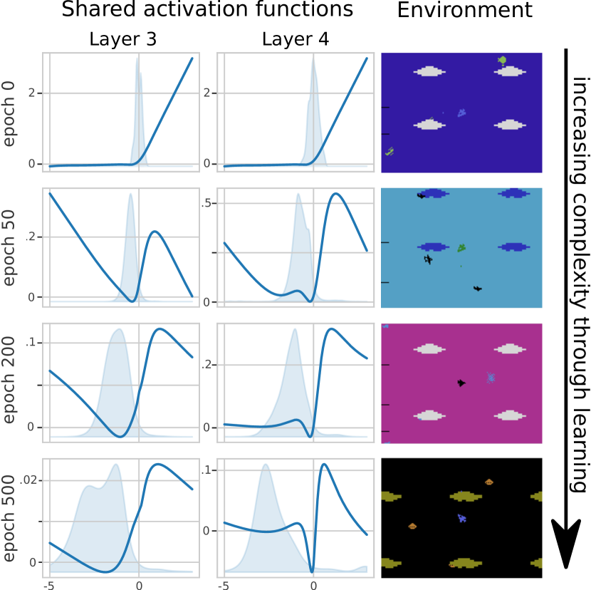
Figure 1: Neural plasticity due to trainable activation functions allows Deep RL agents to adapt to environments of increasing complexity. Rational activations (left columns), with shared parameters in the last two layers, evolve together with their input distributions (shaded blue) when learning with DQN on Time Pilot. Each row corresponds to a state where a new, more challenging part of the environment (right column, e.g. increasing enemy speed and complexity) has been uncovered and is additionally trained on.

1 Introduction

Neural Networks’ efficiency in approximating any function has made them the most used approximation function for many machine learning tasks. This is no different in reinforcement learning (RL), where the introduction of the DQN algorithm (Mnih et al., 2015) has sparked the development of various neural solutions. In concurrence with neuroscientific explanations of brainpower residing in combinations stemming from trillions of connections (Garlick, 2002), present advances have emphasised the role of the neural architecture (Liu et al., 2018; Xie et al., 2019). As such, RL improvements have first been mainly obtained through a focus on enhancing algorithms (Mnih et al., 2016; Haarnoja et al., 2018; Banerjee et al., 2021) and only recently by searching for well-performing architectural patterns (Miao et al., 2021).

However, research has also progressively shown that individual neurons shoulder more complexity than initially expected, with the latest results demonstrating that dendritic compartments can compute complex functions (e.g. XOR) (Gidon et al., 2020), previously categorised as unsolvable by single-neuron systems. This finding seems to have renewed interest in activation functions (Georgescu et al., 2020; Misra, 2020). In fact, many functions have been adopted across different domains (Redmon et al., 2016; Brown et al., 2020; Schulman et al., 2017). To reduce the bias introduced by a fixed activation function and achieve higher expressive power, one can further learn which activation function is performant for a particular task (Zoph & Le, 2017; Liu et al., 2018), learn to combine arbitrary families of activation functions (Manessi & Rozza, 2018), or find coefficients for polynomial activations as weights to be optimised (Goyal et al., 2019).

Whereas these prior approaches have all contributed to their respective investigated scenarios, there exists a finer approach that elegantly encapsulates the challenges brought on by reinforcement learning problems. Specifically, we can learn rational activation functions (Molina et al., 2020). Not only can rational activation functions converge to any continuous function, but they have further been proven to be better approximants than polynomials in terms of convergence (Telgarsky, 2017). Even more crucially, their ability to adapt while learning equips a model with high neural plasticity, i.e. capability to adjust to the environment and its transformations (Garlick, 2002). We argue that adapting to environmental changes is essential, making rational activation functions particularly suitable for dynamic RL environments. To provide a visual intuition, we showcase an exemplary evolution of two rational activation functions together with their respective changing input distributions in the dynamic “Time Pilot” environment in Fig. 1.

In this work, we propose the use of plasticity via rational activations in deep RL agents, as a central element to satisfy the requirements originating from diverse and dynamic environments. Apart from demonstrating the suitability of adaptive activation functions, we further identify and address potential caveats to overcome remaining practical barriers. Our specific contributions are:

(i)

We motivate why neural plasticity is a key aspect for Deep RL agents and that rational activations are adequate as adaptable activation functions. For this purpose, we not only highlight that rational activation functions adapt their parameters over time, but further prove that they can dynamically embed residual connections, which we refer to as residual plasticity.

(ii)

As the introduction of additional representational capacity could hinder generalisation, we then propose a joint rational variant. By making use of weight-sharing across rational activations in different layers, we thus include regularisation, necessary for RL (Farebrother et al., 2018; Roy et al., 2020; Yarats et al., 2021).

(iii)

We empirically demonstrate that the inclusion of rational activations brings significant improvements to DQN and Rainbow algorithms on Atari games and that our joint variant further increases performance.

(iv)

Finally, we investigate the overestimation phenomenon of predicting too large return values, which has previously been argued to originate from an unsuitable representational capacity of the learning architecture (van Hasselt et al., 2016). As a result of our introduced (rational) neural and residual plasticity, such overestimation can practically be reduced.

We proceed as follows. We start off by arguing in favour of plasticity for deep reinforcement learning. Then we show how rational activation functions provide a particularly suitable candidate to provide plasticity in neural networks and present our empirical evaluation. Before concluding, we touch upon related work.

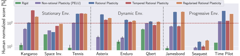
Figure 2: Neural plasticity is essential for reinforcement learning. Human normalised mean scores for rigid DQN agents, agents with non-rational, rational, tempered, and regularised plasticity are shown with standard deviation across 5 random seeded experimental repetitions. Larger scores are better. Tempered plasticity, allowing initial adaptation to the environments, but not their transformations in experimental repetitions, performs better on stationary environments. Regularised plasticity performs well across all environment types. Figure best viewed in colour. A full description of the environments and their types is provided in Appendix A.4.

2 Plasticity via Rational Activation Functions for Deep RL

Let us start by arguing why deep reinforcement learning agents require extensive plasticity and show that parametric rational activation functions provide appropriate means to add such additional plasticity to the network.

As motivated in the introduction, RL is subject to inherent distribution shifts. During the training process, agents progressively uncover new states (input drift) and, as the policy improves, the cumulative reward signal is modified (output drift). More precisely, for input drifts, we can distinguish environments according to how much they change through learning. For simplicity, we categorise according to three intuitive categories: stationary, dynamic and progressive environments. To illustrate, consider the example of Atari 2600 games. Kangaroo, Space Invaders and Tennis can be characterised as stationary since the game’s input distribution does not change significantly. Asterix, Enduro and Q*bert are dynamic environments, as different inputs are provided to the agents early in the game; hence no policy improvement is required to uncover (input) distribution shifts. On the contrary, Jamesbond, Seaquest, and Time Pilot are progressive environments. The agent needs to master early stages before being provided with additional states, i.e. exposed to a significant shift in the input distribution.

How do we efficiently improve RL agents’ ability to adapt to environments and their changes? To deal with these distribution shifts, our agents require high neural plasticity and thus benefit from adaptive architectures. To elaborate further in our work, let us consider the popular DQN algorithm (Mnih et al., 2015), that employs a $\boldsymbol{\theta}$-parameterised neural network to approximate the Q-value function of a state $S_{t}$ and action $a$. This network is updated following the Q-learning equation: $Q\left(S_{t},a;\boldsymbol{\theta}\right)\equiv R_{t+1}+\gamma\max_{a}Q\left(S_{t+1},a;\boldsymbol{\theta}\right)$. In addition to network connectivity playing an important role, we now highlight the importance of individual neurons by modifying the network architecture of the algorithm via the use of learnable activation functions, to show that they are a presently underestimated component. To emphasise the utility of the upcoming proposed rational and joint rational activation functions, we will interleave early results into this section. The latter serves the primary purpose to not only motivate the suitability of the rational parameterisation to provide plasticity, but also discern the individual benefits of (joint-) rational activations, in the spirit of ablation studies.

2.1 Rational Neural Plasticity

A rational function of order $(m,n)$ is a universal approximator, defined by:

$$\operatorname{R}(x)=\frac{\operatorname{P}(x)}{\operatorname{Q}(x)}=\frac{\sum_{j=0}^{m}a_{j}x^{j}}{1+\sum_{k=1}^{n}b_{k}x^{k}}\ ,$$ (1)

where $a_{j}$ and $b_{k}$ are learnable parameters (corresponding to $m\!+\!n\!+\!1$ parameters in total).

In Fig. 2, we show that our proposition to use such a rational parametrisation substantially enhances RL agents. More precisely, by comparing agents with rigid networks (a fixed Leaky ReLU baseline) to agents with rational plasticity (i.e. with a rational activation function at each layer), we see that using rational functions boosts the agents to super-human performances on 7 out of 9 games. The acquired extra neural plasticity seems to play a significant role in these Atari environments, especially in progressive ones.

In order to discern the benefits of general plasticity through any adaptive activation function, over the proposed use of the rational parametrisation, Fig. 2 additionally includes PELU (Trottier et al., 2017). PELU is a parametrised ELU that uses 3 parameters to control its slope, saturation and exponential decay, and has been shown to outperform other learnable alternatives on classification tasks (Godfrey, 2019). However, in contrast to the rational parameterisation, it seems to fall behind and only boosts the agents to super-human performance on 3 out of 9 games (contrary to 7). This implies that the type of parameterisation provided by the rational activation choice is particularly suitable.

To highlight the desirability of rational activations even further, we additionally distinguish between the plasticity of agents towards their specific environment and the plasticity allowing them to adapt while the environment itself is changing. To this end, we also show agents with rational activations that are tempered in Fig. 2. They have been extracted from agents with rational plasticity, that adapted to their specific environment. The plasticity of the rational activation functions is then tempered (“stopped”) in repeated application to emphasise the necessity to continuously adapt during training. Whereas providing agents with such tempered, tailored to the task, activations already boosts performances, rational plasticity at all times seems essential, particularly in the dynamic and progressive environments.

2.2 Rational Residual Plasticity

The prior paragraphs have showcased the advantage of agents equipped with rational activation functions, rooted in their ability to update their parameters over time. However, we argue that the observed boost in performance is not only due to parameters adapting to distributional drifts. In addition to neural plasticity, rational activations can embed one of the most popular techniques to stabilise training of deep neural networks; namely, they can dynamically make use of a residual connection. We refer to this as residual plasticity.

Rationals are closed under residual connection and provide residual plasticity. We here show that using a residual connection together with a rational function is equivalent to using a rational with strictly higher degree in the numerator.

Theorem 2.1.

Let R be a rational activation function of order (m, n). If $m>n$, then R embeds a residual connection.

Proof.

Let us consider a rational function R $=$ P/Q of order $(m,n)$, with coefficients $A^{[m]}=(a_{j})_{j=0}^{m}\in\mathbb{R}^{m+1}$ of P and $B^{[n]}=(b_{i})_{i=0}^{n}\in\mathbb{R}^{n+1}$ of Q (with $b_{0}=1$).
We denote by $\otimes$ (resp. $\oslash$) the Hadamard product (resp. division). Let $X\in\mathbb{R}^{n_{1}\times\dots\times n_{x}}$ be a tensor corresponding to the input of the rational function of an arbitrary layer in a given neural network. We derive $X$${}^{\otimes k}=\bigotimes_{i=1}^{k}$ $X$.
Furthermore, we use $GV^{[k]}(X)=[\textbf{1},X,X^{\otimes 2},...,X^{\otimes k}]\in\mathbb{R}^{(n_{1}\times\dots\times n_{x})\times k+1}$ to denote the tensor containing the powers up to $k$ of the tensor $X$. Note that $GV^{[k]}$ can be understood as a generalised Vandermonde tensor, similar as introduced in (Xu et al., 2016).
For $V^{[k]}\!=\!(v_{i})_{i=0}^{k}\!\in\!\mathbb{R}^{k+1}$, let $GV^{[k]}.V^{[k]}\!=\!\sum_{i=0}^{k}\!v_{i}X^{\otimes i}$ be the weighted sum over the tensor elements of the last dimension.

Now, we apply the rational activation function R with residual connection to $X$:

$$\small\mathbf{y}(X) =\text{R}(X)+X$$

$$=GV^{[m]}(X).A^{[m]}\oslash GV^{[n]}(X).B^{[n]}+X$$

$$=(GV^{[m]}(X).A^{[m]}+X\otimes GV^{[n]}(X).B^{[n]})$$

$$\qquad\qquad\qquad\qquad\oslash GV^{[n]}(X).B^{[n]}$$

$$=(GV^{[m]}(X).A^{[m]}+GV^{[n+1]}(X).B_{0}^{[n+1]})$$

$$\qquad\qquad\qquad\qquad\oslash GV^{[n]}(X).B^{[n]}$$

$$=GV^{[\max(m,n+1)]}(X).C^{[\max(m,n+1)]}$$

$$\qquad\qquad\qquad\qquad\oslash GV^{[n]}(X).B^{[n]}$$

$$=\widetilde{\text{R}}(X),$$

where $B_{0}^{[n+1]}=(b_{0,i})_{i=0}^{n+1}\in\mathbb{R}^{n+2}$ (with $b_{0,0}=0$ and $b_{0,i}=b_{i-1}$ for $i\in\{1,\makebox[6.99997pt][c]{.\hfil.\hfil.},n+1\}$),
$C^{[\max(m,n+1)]}=(c_{j})_{j=0}^{\max(m,n+1)}$ with $c_{j}=a_{j}+b_{j-1}$, $a_{j}\!=\!0$ for all $j\!\notin\!\{0,\makebox[6.99997pt][c]{.\hfil.\hfil.},m\}$ and $b_{j}\!=\!0$ for all $j\!\notin\!\{0,\makebox[6.99997pt][c]{.\hfil.\hfil.},n\}$.
$\widetilde{\text{R}}$ is a rational function of order $(m^{\prime},n^{\prime})$, with $m^{\prime}>n^{\prime}$. ∎

In other words, rational activation functions of order $m>n$ can embed residual connections if necessary. Using the same degrees for numerator and denominator certifies asymptotic stability, but our derived configuration allows rationals to implicitly use residual connections. Importantly, note that these potential residual connections are not rigid, as these functions can progressively learn $a_{j}\!=\!0$ for all $j\!>\!n$, i.e. we have residual plasticity.

Rationals to potentially replace residual blocks. Recall that residual neural networks (ResNets) were initially introduced following the intuition that it is easier to optimise the residual mapping than to optimise the original, unreferenced mapping (He et al., 2016). Formally, residual blocks of ResNets propagate an input $X$ through two paths: a transforming block of layers that preserves the dimensionality ($F$) and a residual connection (identity). In very deep ResNets, it has been observed that feature re-combinations does not occur inside the residual blocks but that transitions to new levels of representations occur during dimensionality changes (Veit et al., 2016; Greff et al., 2017).

To investigate this hypothesis, Veit et al. have conducted lesioning experiments, where a residual block is removed from the network, and surrounding ones are fine-tuned to recover. Whereas we emphasize that we do not claim that the residual in rationals can replace entire convolutional blocks or that they are generally equivalent, we hypothesize that under the conditions investigated by Veit et al. of very deep networks, residual blocks could learn complex activation function-like behaviours. To test this conjecture, we repeat the lesioning experiments, but also test replacing the lesioned block with a rational function that satisfies the residual connection condition derived above. Results are provided in appendix (cf. A.1) and show that such rational functions can efficiently replace some residual blocks of very deep ResNets.

2.3 Natural Rational Regularisation

We have motivated and shown that the combination of neural and residual plasticity form the central pillars for why rational activation functions are desirable in deep RL. In particular for dynamic and progressive environments, rational plasticity has been observed to provide a substantial boost over alternatives. However, if we circle back to this figure and take a more careful look at the stationary environments, we can observe that our previously investigated tempered rational plasticity (for emphasis, initially allowed to tailor to the task but later “stopped” in experimental repetition) can also have an upper edge over full plasticity. The extra rational plasticity at all times might reduce the generalisation capabilities of its agents, particularly on non-diverse stationary environments. In fact, prior works have highlighted the necessity for regularisation methods in RL (Farebrother et al., 2018; Roy et al., 2020; Yarats et al., 2021).

We thus propose a naturally regularised rational activation version. For this regularised variant, we again draw inspiration from residual blocks. In particular, Greff et al. have indicated that sharing the weights can improve learning performances, as shown in Highway (Lu & Renals, 2016) and Residual Networks (Liao & Poggio, 2016). In the spirit of these findings, we propose the regularised joint rationals, where the key idea is to constraint the input to propagate through different layers but always be activated by the same learnable rational activation function. Rational functions thus share a mutual set of parameters across the network. As observable in Fig. 2, this regularised form of plasticity increases the agents’ scores in the stationary environments and does not deteriorate performances in the progressive ones.

Table 1: Neural plasticity leads to vast performance improvements. Normalised mean scores and standard deviations (in percentage, cf. Appendix A.6 for the equation) of rigid baselines (i.e. DQN and DDQN with Leaky ReLU, DQN with SiLU and SiLU + dSiLU), as well as DQN with plasticity: using PELU, rational (full) and joint-rational (regularised), are reported over five experimental random seeded repetitions (larger mean values are better). The best results are highlighted in bold and runner-ups denoted with $\bullet$ markers. The last rows summarise the number of times best mean scores were obtained by each agent and the number of super-human performances.

Algorithm	DQN			DDQN	DQN with Plasticity
Activation	LReLU	SiLU	d+SiLU	LReLU	PELU	rational	joint-rational
Asterix	1.85$\pm$1.2	0.52$\pm$0.6	2.14$\pm$1.4	48.9$\pm$17.7	25.8$\pm$3.7	242$\pm$23.5	168$\pm$32.6$\bullet$
Battlezone	11.4$\pm$7.0	21.2$\pm$15.0	11.3$\pm$6.7	68.2$\pm$34.8	46.6$\pm$19.5	70.1$\pm$2.1$\bullet$	77.4$\pm$8.7
Breakout	558$\pm$166	93.9$\pm$57.6	11.7$\pm$14.0	286$\pm$122	788$\pm$79.2	1134$\pm$130$\bullet$	1210$\pm$36.0
Enduro	16.3$\pm$21.3	37.0$\pm$17.7	0.37$\pm$0.5	47.7$\pm$18.1	24.5$\pm$42.6	141$\pm$15.0	129$\pm$14.7$\bullet$
Jamesbond	8.62$\pm$6.4	6.08$\pm$3.7	5.28$\pm$4.4	10.7$\pm$11.1	74.2$\pm$51.5	308$\pm$48.5$\bullet$	312$\pm$59.5
Kangaroo	11.8$\pm$12.5	128$\pm$95.6$\bullet$	13.9$\pm$18.5	17.2$\pm$14.5	57.7$\pm$14.6	107$\pm$43.1	193$\pm$86.8
Pong	101$\pm$5.5	96.1$\pm$12.0	104$\pm$3.3	91.3$\pm$30.8	106.4$\pm$2.2	107.0$\pm$2.4$\bullet$	107.3$\pm$2.7
Qbert	55.4$\pm$17.1	14.2$\pm$17.0	2.74$\pm$0.2	74.0$\pm$21.7	101$\pm$6.6	120$\pm$2.8	117$\pm$4.9$\bullet$
Seaquest	0.57$\pm$0.4	3.67$\pm$4.1	0.18$\pm$0.2	2.17$\pm$0.9	9.21$\pm$2.5	16.3$\pm$0.5$\bullet$	18.4$\pm$3.3
Skiing	-90.7$\pm$37.9	-111$\pm$-0.7	-85.5$\pm$43.4	-86.9$\pm$46.6	-111$\pm$-.7	-59.5$\pm$60.7	-60.2$\pm$56.1$\bullet$
Spaceinvaders	33.9$\pm$4.3	33.1$\pm$11.9	32.4$\pm$12.4	31.0$\pm$1.0	50.1$\pm$3.3$\bullet$	42.3$\pm$3.1	95.1$\pm$17.7
Tennis	8.94$\pm$17.3	26.3$\pm$53.3	78.5$\pm$64.3	32.1$\pm$51.6	106$\pm$53.3	257.8$\pm$2.8$\bullet$	258.3$\pm$5.2
Timepilot	14.9$\pm$14.3	19.3$\pm$31.0	18.3$\pm$38.1	6.61$\pm$7.5	124$\pm$26.1	341$\pm$105	253$\pm$11.0$\bullet$
Tutankham	0.03$\pm$2.8	58.2$\pm$48.6	2.89$\pm$4.0	24.4$\pm$-0.4	91.6$\pm$29.3	130$\pm$10.7$\bullet$	134$\pm$29.3
Videopinball	440$\pm$123	55.8$\pm$61.9	-4.03$\pm$32.5	626$\pm$241	299$\pm$168	1616$\pm$1026	906$\pm$539$\bullet$
# Wins	0/15	0/15	0/15	0/15	0/15	6/15	9/15
# Super-Human	3/15	1/15	1/15	2/15	6/15	11/15	11/15

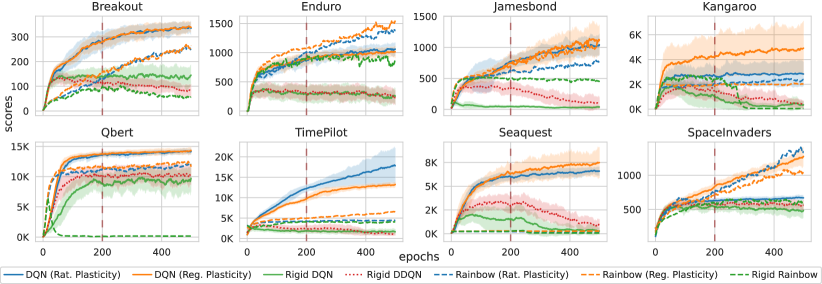
Figure 3: Networks with rational (Rat.) and regularized (Reg.) rational plasticity compared to rigid baselines (DQN, DDQN and Rainbow) over five random seeded runs on eight Atari 2600 games. The resulting mean scores (lines) and standard deviation (transparent area) during training are shown. As one can see, DDQN does not resolve performance drops but only delays them (e.g. particularly pronounced on Seaquest). A figure including the evolution of every agent on all Atari 2600 games is provided in Appendix A.3. Best viewed in colour.

3 Empirical Evidence for Plasticity

Our intention here is to investigate the benefits of neural plasticity through rational networks for deep reinforcement learning. That is, we investigated the following questions:

(Q1)

Do neural networks equipped with rational plasticity outperform rigid baselines?

(Q2)

Can neural plasticity make up for more heavy algorithmic RL advancements?

(Q3)

Can plasticity address the overestimation problem?

(Q4)

As plasticity can be obtained via adding parameters, how many more parameters would rigid networks need to measure up to rational ones?

To this end, we compare our rational networks using the original DQN algorithm (Mnih et al., 2015) on 15 different games of the Atari 2600 domain (Brockman et al., 2017) and compare these architectures to ones equipped with the Leaky ReLU baseline, the learnable PELU, as well as SiLU ($\operatorname{SiLU}(x)=x\cdot\operatorname{sigmoid}(x)$) and its derivative dSiLU. Elfwing et al. showed that SiLU or a combination of SiLU (on convolutional layers) and its derivative (on fully connected layers) perform better than ReLU in DQN agents on several games (2018). SiLU and dSiLU are —to our knowledge— the only activation functions specifically designed for RL applications. We then compare increased neural plasticity provided by (joint-)rational networks to algorithm improvements, namely the Double DQN (DDQN) method (van Hasselt et al., 2016), that tackles DQN’s overestimation problem, as well as Rainbow (Hessel et al., 2018). Rainbow incorporates multiple algorithm improvements brought to DQN—Double Q-learning, prioritised experience replay, duelling network architecture, multi-step target, distributional learning and stochastic networks—and is widely used also as a baseline (Lin et al., 2020; Hafner et al., 2021). We further explain how neural plasticity can help readdress overestimation. Finally, we evaluate the number of additional weights needed by rigid networks to approximate rational ones.

In practice, we used safe rational activation functions (Molina et al., 2020), i.e. we used the absolute value of the sum in the denominator to avoid poles. This stabilises training and makes the function continuous without creating instabilities. Rationals are shared across layers (adding only $10$ parameters per layer) or through the whole network for the regularised version. We base our experiments on the original neural networks used by the DQN, DDQN and SiLU authors and the same hyper-parameters (cf. Appendix A.6.2) across all the Atari agents. For a fair comparison, we report performances using the normalised (cf. Eq. 4 in Appendix) mean and standard deviation of the scores obtained by fully trained agents over five seeded reruns for every (D)DQN agent. However, since often only the best performing RL agent (among the reruns) is reported in the literature, we also provide tables of such scores (cf. Appendix A.2). For the Rainbow algorithm, we unfortunately can only report the results of single runs. A single run took more than 40 days on an NVIDIA Tesla V100 GPU; Rainbow is known to be computationally quite demanding (Obando-Ceron & Castro, 2021).

(Q1) DQN with neural plasticity is better than rigid baselines. To start off, we compared RL agents with additional plasticity (from PELU and rationals) to rigid DQN baselines: Leaky ReLU, as well as agents equipped with SiLU and SiLU+dSiLU activation functions.

The results summarised in Tab. 1 confirm what our earlier figure had shown, but on a larger scale. As one can see, DQN agents with plasticity clearly outperform their rigid activation counterparts. Furthermore, RL agents with functions of the SiLU family outperform Leaky ReLU ones on less than half of the tested games. More importantly, they do not perform better than non-rigid rational networks. DQN with regularised plasticity even obtains higher mean scores than the non-regularised versions 9 out of 15 times. Actually, DQN with non-rational plasticity (PELU) obtained super-human performances on 6 out of 15 games, in contrast to the 11 out of 15 times of agents with rational plasticity.

This clearly shows that plasticity, and above all rational plasticity pays off for (deep) RL agents, providing an affirmative answer to Q1.

(Q2) DQN with neural plasticity can beat more complex RL approaches such as Rainbow.

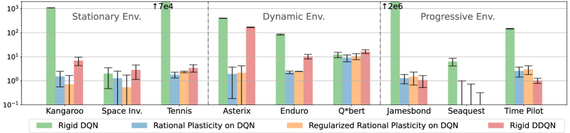
Figure 4: Plasticity naturally reduces overestimation. Relative overestimation values (log scale, smaller values are better, see Eq. 2) of both rigid DQN and DDQN, as well as DQN with rational and regularised rational plasticity. Each trained agent is evaluated on 100 completed games (5 random seeds per game per agent, i.e. 20 completed games for each seed). Agents with rational plasticity lower overestimation values as much or further than rigid DDQN ones, which has specifically been introduced to this end. Figure best viewed in colour.

Fig. 3 shows the learning curves of Rainbow and DQN, both with Leaky ReLU baselines, as well as with full and regularised plasticity. While Rainbow is computationally much heavier ($\sim 8$ times slower than DQN in our experiments, with higher memory needs), its rigid form never outperforms the much simpler and more efficient DQN with neural plasticity, and its rational versions dominate in only 1 out of 8 games (Enduro). Rainbow even lost to vanilla DQN on 3 games.

Therefore, DQN agents with rational plasticity are competitive alternatives to the complicated and expensive Rainbow method, answering question (Q2) affirmatively.

(Q3) Neural plasticity directly tackles the overestimation problem. Revisiting Fig. 3, one can see that Rainbow variants are worst on dynamic environments such as Jamesbond, Time Pilot and particularly Seaquest. For these games, the performance of rigid (Leaky ReLU) DQN progressively decreases.

Such drops are well known in the literature and are typically attributed to the overestimation problem of DQN. This overestimation is due to the combination of bootstrapping, off-policy learning and a function approximator (neural network) operating by DQN. van Hasselt et al. showed that inadequate flexibility of the function approximator (either insufficient or excessive) can lead to a slight overestimation of a state-action pair (2016). The max operator in the update rule of DQN then propagates this overestimation while learning with the replay buffer. The overestimated states can stay in the buffer long before the agent revisit (and thus update) them. This can lead to catastrophic performance drops. To mitigate this problem, van Hasselt et al. introduced a second network to separate action selection from action evaluation, resulting in Double DQN (DDQN).

We have compared the original DDQN approach (i.e. equipped with Leaky ReLU), which is rigid, to vanilla DQN with neural plasticity on Atari games. As one can see in Tab. 1, DQN with rational plasticity even outperforms the more complex DDQN algorithm on every considered Atari game. This reinforces the affirmative answer to (Q1) from earlier on.

More importantly, we have computed the relative overestimation values of the (D)DQN, both with and without neural plasticity, following:

$$\text{overestimation}=\frac{\text{Q-value}-R}{R},$$ (2)

where the return $R$ corresponds to $R=\sum_{t=0}^{\infty}{\gamma^{t}r_{t}}$, with the observed reward $r_{t}$ and the discount factor $\gamma$.

The results are summarised in Fig. 4. As one can see, plasticity helps to reduce overestimation drastically. The game for which DDQN substantially reduces the overestimation are Jamesbond, Kangaroo, Tennis, Time Pilot and Seaquest. For these games, DDQN obtains the best performances among all rigid variants only on Jamesbond (cf. Tab. 1). Moreover, Fig. 3 reveals that the performance drops of corresponding DDQN rigid agents are only delayed and not prevented. The performance drops thus happen after the 200th epoch, after which the training of RL agents is usually stopped.

Whereas we agree that overestimation might play a role in the performance drops on progressive environments (cf. Fig. 3: Jamesbond, TimePilot and Seaquest), it cannot fully explain the phenomena. Instead, RL agents with higher neural plasticity can handle these games much better while only having a few more parameters. Hence, we advocate that neural plasticity better deals with distribution shifts due to the dynamics of games with progressive environments.

Perhaps surprisingly, (regularised) rational plasticity not only works well on challenging progressive environments but also on much simpler ones such as Enduro, Pong and Q*bert, where more flexibility is likely to hurt. Luckily, overestimation due to high flexibility does not happen here, as one can see in Fig. 4. Moreover, the activation functions learned for these games have a simpler profile than those learned on more complicated games like Kangaroo and Time Pilot (cf. Appendix A.5). The rational activation functions thus seem to adapt to the environment’s complexity and the policy they need to model. This clearly provides an affirmative answer to (Q3).

(Q4) Adding parameters through rationals efficiently augments plasticity. Compared to rigid alternatives, the joint-rational networks embed $10$ more parameters in total and always outperform (cf. Tab. 1) PELU ones (that have 12 additional parameters). Our proposed method to add plasticity via rational activation functions thus efficiently augments the capacity of the network. However, ReLU layers can theoretically approximate rational functions (Telgarsky, 2017). Augmenting the number of layers (or neurons per layer) is thus, theoretically, a costly alternative to augment the plasticity. How many parameters are practically needed in rigid networks to obtain similar performances? Searching for bigger equivalent architectures for RL agents is tedious, as RL training curves possess considerably more variance and noise than SL ones (Miao et al., 2021), but this question is not restricted to reinforcement learning. We thus answer it by highlighting the generality of our insights, demonstrated by further investigation on a classification scenario, in addition to the RL experiments of Tab 1. We report our findings in Tab. 2, where networks with rational activations are shown to not only outperform Leaky ReLU ones at the same amount of parameters, but also to outperform deeper and more heavily parametrised neural networks (indicated by the pairs of colours). For example, a rational activated VGG4 not only performs better than a rigid Leaky ReLU VGG4 at 1.37M parameters, but even performs similarly to the 4.71M parameters VGG6 that uses Leaky ReLU.

Table 2: Shallow Rational Networks perform as deeper Leaky ReLU ones. VGG networks with different numbers of layers are evaluated on CIFAR10 and CIFAR100. Rational VGG4 has similar performances as VGG6 network, with $3.5$ times less parameters, and Rational VGG6 outperforms VGG8, with two times less parameters. Shaded colour pairs included for emphasis.

Architecture		VGG4		VGG6		VGG8
Activation		LReLU	Rat.	LReLU	Rat.	LReLU	Rat.
C10	Train	83.0±.3	87.1±.6	86.9±.1	89.2±.2	86.7±.2	89.2±.1
	Test	80.0±1.	84.3±.5	83.2±.6	85.4±.6	83.4±1.	85.8±.9
C100	Train	64.7±.8	70.2±.0	70.6±.6	75.4±.1	71.8±.3	74.3±.3
	Test	56.6±.8	58.9±.6	59.0±.5	58.4±.3	57.1±1.	59.1±.9
# Net params		1.37M		4.71M		9.27M

All experimental results together clearly show that neural plasticity through rational networks considerably benefits deep reinforcement learning in highly efficient manner.

4 Related Work

Next to the related work discussed throughout the paper, our work on plasticity is also related to research lines on neural architecture search and activation functions in deep reinforcement learning.

Neural Architectures for Deep Reinforcement Learning. Cobbe et al. showed that the architecture of IMPALA (Espeholt et al., 2018), notably containing residual blocks, improved the performances over the original Nature-CNN network used in DQN (2019). Motivated by these findings, (Miao et al., 2021) recently applied neural architecture search to RL tasks and demonstrated that the optimal architecture and its complexity highly depend on the environment. Their search provides different architectures for different environments, with varying activation functions across layers and potential residual connections. Continuously modifying the complexity of the neural network based on the noisy reward signal in a complex architectural space is extremely resource demanding, particularly for large scale problems. Many RL specific problems, such as noisy rewards (Henderson et al., 2018), input interdependency (Mnih et al., 2015), policy instabilities (Haarnoja et al., 2018), sparse rewards, difficult credit assignment (Mesnard et al., 2021), complicate an automated architecture search.

The choice of activation functions. Many different activation functions have been adopted across different domains (e.g. Leaky ReLU in YOLO (Redmon et al., 2016), Tanh in PPO (Schulman et al., 2017), GELU in GPT-3 (Brown et al., 2020)), indicating that the relationship between the choice of activation functions and performance of neural networks is highly dependent on the task, architecture, hyper-parameters and the dataset (or environment). As shown in this paper, parametric functions provide plasticity. Molina et al. showed that rationals outperform other learnable activation function types on a set of SL tasks (2020). Telgarsky showed that rationals are locally better approximants than polynomials (2017). Finally, Boullé et al. later showed that composing low-degree rational functions require fewer parameters to approximate a ReLU Network (2020). While this is indeed more efficient in terms of parameters, compositions of rationals functions need to be computed sequentially, which is slower when using gradient descent methods.

5 Limitations and Future Work

We have shown the benefits of rational activation functions for deep RL as a consequence of both their neural and residual plasticity. In our derivation for closure under residuals, we have deduced that the degree of the polynomial in the numerator needs to be greater than that of the denominator. Correspondingly, we have based our empirical investigations on the degrees (5, 4). Interesting future work would be to further automatically select suitable degrees that fulfil this condition. As additional future avenues, one should also explore neural plasticity in more advanced deep RL approaches, including short term memory (Kapturowski et al., 2019), finer exploration strategy (Badia et al., 2020), or include neural plasticity into architecture search, without having to perform a combinatorial search across possible activation functions.

6 Conclusion

In this work, we have highlighted the central role of neural plasticity in deep reinforcement learning algorithms, and have motivated the use of rational activation functions, as a lightweight way of boosting RL agents performances. We derived a condition, under which rational functions embed residual connections. Then the naturally regularised joint-rational activation function was developed inspired by weight sharing in residual networks.

The simple DQN algorithm equipped with these (regularised) rational forms of plasticity becomes a competitive alternative to more complicated and costly algorithms, such as Double DQN and Rainbow. Fortunately, the complexity of these rational functions also seem to automatically adapt to the one of the environment used for training. Their use could be a substitute for more expensive architectural searches. We thus hope that they will be adopted in future deep reinforcement learning algorithms, as they can provide agents with the necessary neural plasticity required by stationary, dynamic and progressive reinforcement learning environments.

Appendix A Appendix

As mentioned in the main body, the appendix contains additional materials and supporting information for the following aspects: results on replacing residual blocks with rational activation functions (A.1), every final and maximal scores obtained by the reinforcement learning agents used in our experiments (A.2), the evolutions of these scores (A.3), the different environment types with illustrations of their changes (A.4), graphs of the learned rational activation functions (A.5) and technical details for reproducibility (A.6).

A.1 Residual block learn of deep ResNet learn activation function-like behavior.

We present in this section lesioning experiments, where a residual block is lesioned from a pretrained Residual Network, and the surrounding blocks are fine-tuned (with a learning rate of $0.001$) for $15$ epochs. These lesioning experiments were first conducted by Veit et al. (2016). We also perform rational lesioning, where we replace a block by an (identity initialised) rational activation function (instead of removing the block), and train the activation function along with the surrounding blocks. The used rational functions have the same order as in every other experiment ($(m,n)=(5,4)$), that satisfies the rational residual property derive in the paper). We report recovery percentages, computed following:

$$\text{recovery}=100\times\frac{\text{finetuned}-\text{surgered}}{\text{original}-\text{surgered}}.$$ (3)

We also provide the amount of dropped parameters of each lesioning.

Table 3: Rational functions improve lesioning. The recovery percentages for finetuned networks after lesioning (Veit et al., 2016) of a ResNet layer’s (L) block (B) are shown. Residual blocks were lesioned, i.e. replaced with the identity (Base) or a rational from a pretrained ResNet101 (44M parameters). Then, the surrounding blocks (and implanted rational activation function) are retrained for 15 epochs. Larger percentages are better, best results are in bold.

Recovery (%)	Lesioning	L2B3	L3B19	L3B22	L4B2
Training	Original (Veit et al., 2016)	100.9	90.5	100	58.9
	Rational (ours)	101.1	104	120	91.1
Testing	Original (Veit et al., 2016)	93.1	97.1	81.6	81.7
	Rational (ours)	90.5	97.6	91.5	85.3
% dropped params		0.63	2.51	2.51	10.0

As the goal is to show that flexible rational functions can achieve similar modelling capacities to the residual blocks, we did not apply regularisation methods and mainly focused on training accuracies. We can clearly observe that rational activation functions lead to performance improvements that even surpass the original model, or are able to maintain performances when the amount of dropped parameters rises.

A.2 Complete raw scores table for Deep Reinforcement Learning

Through this work, we showed the performance superiority of reinforcement learning agents that embed additional plasticity provided by learnable rational activation functions. We used human normalised scores (cf. Eq. 4) for readability. For completeness, we provide in this section the final raw scores of every trained agent. As many papers provide the maximum obtained score among every epoch and every agent, even if we consider it to be an inaccurate and noisy indicator of the performances, for which random actions can still be taken (because of $\epsilon$-greedy strategy also being used in evaluation). A fairer indicator to compare methods is the mean score. We thus also provide final mean scores (of agents retrained among 5 seeded reruns) with standard deviation. We start off by providing the human scores used for normalisation (provided by van Hasselt et al., in Table 5), then provide final mean and maximum obtained raw scores of every agent.

Human scores used for normalisation:
Asterix: $7536$,    Battlezone: $33030$,    Breakout: $27.9$,    Enduro: $740.2$,    Jamesbond: $368.5$,    Kangaroo: $2739$,    Pong: $15.5$,    Q*bert: $12085$,    Seaquest: $40425.8$,    Skiing: $-3686.6$,    Space Invaders: $1464.9$,   Tennis: $-6.7$,    Time Pilot: $5650$,    Tutankham: $138.3$,    Video Pinball: $15641.1$

Final mean scores of other agents:

Algorithm	Random	DQN			DDQN	DQN with Plasticity
Network type	-	LReLU	SiLU	d+SiLU	LReLU	PELU	full	regularised
Asterix	67.9$\pm$2.2	206$\pm$90	107$\pm$45	228$\pm$108	3723$\pm$1324	1998$\pm$275	18109$\pm$1755	12621$\pm$2436
Battlezone	788$\pm$38	4464$\pm$2291	7612$\pm$4877	4429$\pm$2183	22775$\pm$11265	15807$\pm$6320	23403$\pm$701	25749$\pm$2837
Breakout	0.14$\pm$01	155$\pm$46	26.2$\pm$16	3.4$\pm$3.89	79.4$\pm$33.8	219$\pm$22	315$\pm$36	336$\pm$10
Enduro	0$\pm$0	121$\pm$158	274$\pm$131	2.77$\pm$3.41	353$\pm$134	181$\pm$315	1043$\pm$111	957$\pm$109
Jamesbond	6.39$\pm$0.41	37.6$\pm$23.6	28.4$\pm$13.8	25.5$\pm$16.2	45.2$\pm$40.7	275$\pm$187	1122$\pm$176	1137$\pm$216
Kangaroo	14.2$\pm$0.9	335$\pm$342	3500$\pm$2607	393$\pm$504	484$\pm$395	1586$\pm$398	2940$\pm$1175	5266$\pm$2365
Pong	-20.2$\pm$0	15.9$\pm$2	14.1$\pm$4.3	16.9$\pm$1.2	12.4$\pm$11	17.8$\pm$0.8	18$\pm$0.9	18.1$\pm$1
Q*bert	40.6$\pm$2.8	6715$\pm$2058	1754$\pm$2048	371$\pm$28	8954$\pm$2616	12143$\pm$795	14436$\pm$336	14080$\pm$593
Seaquest	20.1$\pm$0.4	250$\pm$162	1504$\pm$1677	94.6$\pm$87.2	898$\pm$353	3740$\pm$991	6603$\pm$200	7461$\pm$1321
Skiing	-16104$\pm$92	-27365$\pm$4794	-29890$\pm$4	-26725$\pm$5485	-26892$\pm$5881	-29912$\pm$10	-23487$\pm$7624	-23582$\pm$7058
Space Inv.	51.6$\pm$1.1	531$\pm$62	520$\pm$169	509$\pm$176	490$\pm$15	759$\pm$48	650$\pm$45	1395$\pm$251
Tennis	-23.9$\pm$0.0	-22.4$\pm$3.0	-19.4$\pm$9.2	-10.4$\pm$11.1	-18.4$\pm$8.9	-5.6$\pm$9.2	20.5$\pm$0.5	20.6$\pm$0.9
TimePilot	688$\pm$30	1428$\pm$739	1644$\pm$1566	1594$\pm$1918	1016$\pm$401	6818$\pm$1323	17632$\pm$5242	13261$\pm$576
Tutankham	3.51$\pm$0.54	3.55$\pm$4.3	81.9$\pm$66	7.41$\pm$5.96	36.4$\pm$0	127$\pm$40	179$\pm$15	184$\pm$40
VideoPinb.	6795$\pm$461	45683$\pm$11383	11730$\pm$5941	6439$\pm$3336	62151$\pm$21791	42051$\pm$15356	149712$\pm$91219	86942$\pm$48143

Table 4: Final mean raw scores (with std. dev.) of rigid baselines (i.e. DQN and DDQN with Leaky ReLU, DQN with SiLU and SiLU + dSiLU), as well as DQN with full plasticity (i.e. using rational activation functions) and regularised plasticity (i.e. using joint-rational ones) on Atari 2600 games, averaged over $5$ seeded reruns (larger mean values are better).

Maximum obtained scores:

Algorithm	Random	DQN			DDQN	DQN with Plasticity
Network type	-	LReLU	SiLU	d+SiLU	LReLU	PELU	full	regularised
Asterix	71	9250	3400	3800	20150	9300	84950	49700
Battlezone	843	88000	81000	70000	97000	68000	78000	94000
Breakout	0	427	370	344	411	430	864	864
Enduro	0	1243	928	1041	1067	1699	1946	1927
Jamesbond	6	5600	5750	700	7500	6150	9250	13300
Kangaroo	15	14800	15600	10200	13000	12400	16200	16800
Pong	-20	21	21	21	21	21	21	21
Q*bert	45	19425	11700	5625	19200	18900	24325	25075
Seaquest	20	7440	8300	740	15830	14860	9100	26990
Skiing	-15997	-5987	-6505	-6267	-5359	-5495	-5368	-5612
Space Inv.	53	2435	2205	2460	2290	2030	2490	3790
Tennis	-23	8	1	-1	4	-1	24	36
Time Pilot	730	11900	15500	12500	12200	16300	72000	28000
Tutankham	4	249	267	267	274	397	334	309
VideoPinb.	7599	998535	950250	338512	991669	322655	997952	998324

Table 5: Maximum obtained scores (with std. dev.) of rigid baselines (i.e. DQN and DDQN with Leaky ReLU, DQN with SiLU and SiLU + dSiLU), as well as DQN with full plasticity (i.e. using rational activation functions) and regularised plasticity (i.e. using joint-rational ones) on Atari 2600 games, averaged over $5$ seeded reruns (larger values are better).

Final mean and maximum obtained scores of Rainbow agents:

Evaluation	Final Mean Scores			Max. Obtained Scores
Plasticity	rigid	full	regularised	rigid	full	regularised
Breakout	52	279	303	383	569	569
Enduro	844	1473	1470	1388	1973	1964
Kangaroo	40	2157	2139	6300	6000	4800
Q*bert	149	11931	11551	16125	23550	23550
Seaquest	82	247	282	920	1280	1280
Space Inv.	595	1263	1157	2070	3395	2875
Time Pilot	3926	5386	6411	12700	15900	15900

Table 6: Final mean and maximum obtained scores obtained by rigid Rainbow agents (i.e. using Leaky ReLU), as well as Rainbow with full (i.e. using rational activation functions) and regularised (i.e. using joint-rational ones) plasticity (only 1 run because of computational cost, larger values are better).

A.3 Evolution of the scores on every game

The main part present some graphs that compares performance evolutions of the Rainbow and DQN agents with plasticity, as well as Rigid DQN, DDQN and Rainbow agents. We provide hereafter the evolution of the scores of every tested DQN and the DDQN agents on the complete game set. DQN agents with higher plasticity are always the best-performing ones. Experiments on several games (e.g. Jamesbond, Seaquest) show that using DDQN does not prevent the agent’s performance drop but only delays it.

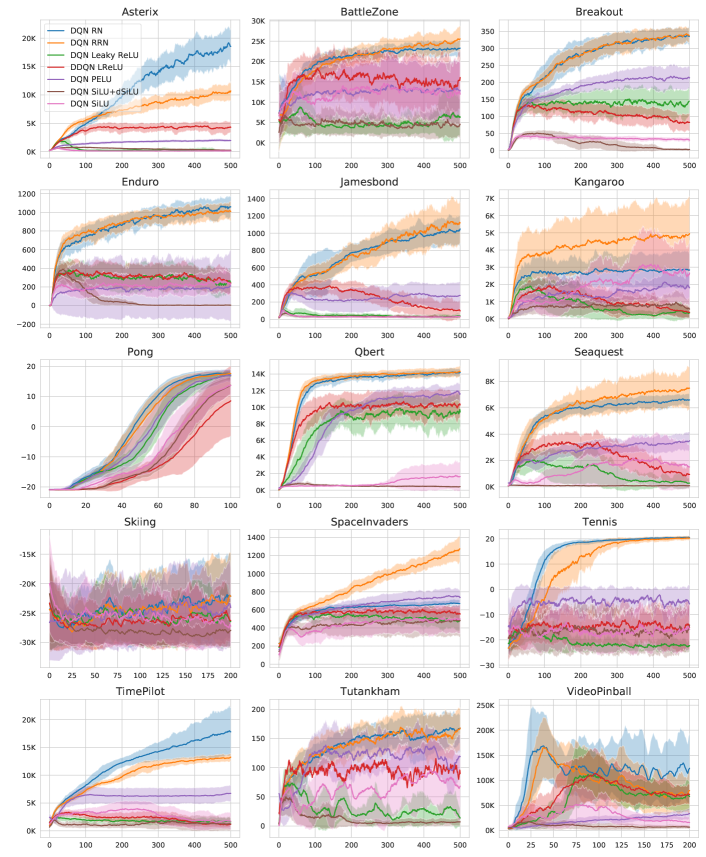
Figure 5: Smoothed (cf. Eq. 5) evolutions of the scores on every tested game for DQN agents with full (i.e. using rational activation functions) and regularised (i.e. using joint-rational ones) plasticity, and original DQN agents using Leaky ReLU, SiLU and SiLU+dSiLU, as well as for DDQN agents with Leaky ReLU.

A.4 Environments types: stationary, dynamics and progressive

The used environments have been separated in 3 categories, describing their potential changes through agents learning. This categorisation is here illustrated with frames of the tested games. As one can see: Breakout, Kangaroo, Pong, Skiing, Space Invaders, Tennis, Tutankham and VideoPinball can be categorised as stationary environment, as changes are minimal for the agents in these games. Asterix, BattleZone, Q*bert and Enduro present environment changes, that are early reached by the playing agents, and are thus dynamic environments. Finally, Jamesbond, Seaquest and Time Pilot correspond to progressive environments, as the agents needs to master early changes to access new parts of these environments.

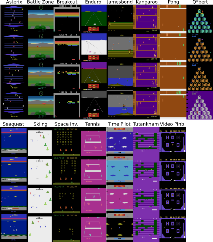
Figure 6: Images extracted from DQN agents with full plasticity playing the set of 15 Atari 2600 games used in this paper. Stationary environments (e.g. Pong, Video Pinball) do not evolve during training, dynamic ones provide different input/output distributions that are early accessible in the game (e.g Q*bert, Enduro) and progressive ones (e.g. Jamesbond, Time Pilot) require the agent to improve for the it to evolve.

A.5 Learned rational activation functions

We have explained in the main text how rational functions of agents used on different games can exhibit different complexities. This section provides the learned parametric rational functions learned by DQN agents with full plasticity (left) and by those with regularised plasticity (right) after convergence for every different tested game of the gym Atari 2600 environment. Kernel Density Estimations (with Gaussian kernels) of input distributions indicates where the functions are most activated. Rational functions from agents trained on simpler games (e.g. Enduro, Pong, Q*bert) have simpler profiles (i.e. fewer distinct extremas).

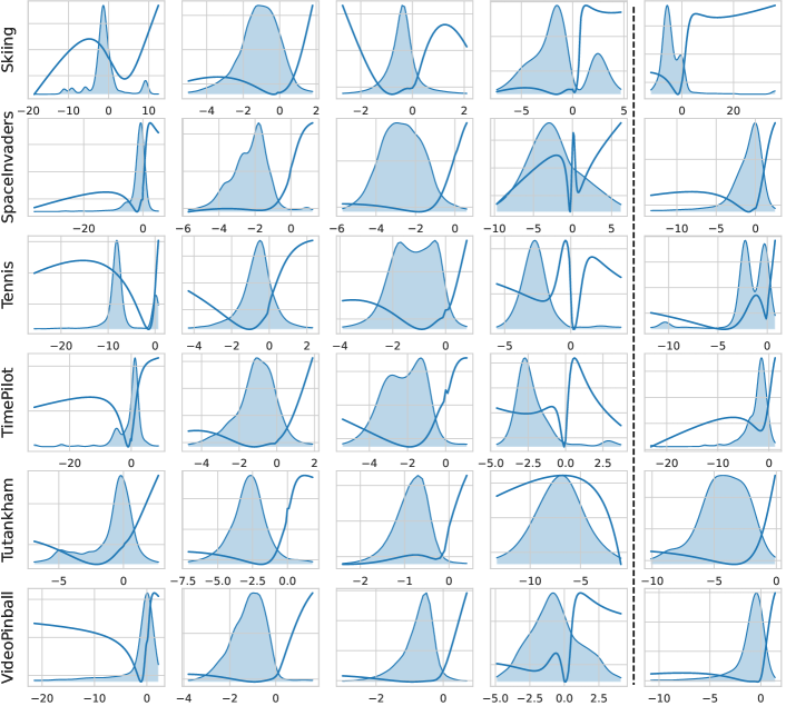
Figure 7: Profiles (dark blue) and input distributions (light blue) of rational functions (left) and joint-rational ones (right) of DQN agents on the different tested games. (Joint-)rational functions from agents of simpler games have simpler profiles (i.e. fewer distinct extrema).

A.6 Technical details to reproduce the experiments

We here provide details on our experiments for reproducibility.

A.6.1 Supervised Learning Experiments

For the lesioning experiment, we used an available pretrained Residual Network (original). We then remove the corresponding block (and potentially replace it with an identity initialised rational activation function) (surgered). We finetune the new models, allowing for optimisation of the previous and next layers (and potentially the rational function) for $15$ epochs with SGD (learning rate of $0.001$).

For the classification experiments conducted on CIFAR10 and CIFAR100, we let every network learn for $60$ epochs. We use SGD as the optimisation algorithm, with a learning rate of $0.02$ and $128$ as batch size. The VGG networks contain successive VGG blocks that all consist of $n$ convolutional layers, $i$ input channels and $o$ output channels, stride $3$ and padding $1$, followed by an activation function, and $1$ Max Pooling layer. For each used architecture, the ($n$, $i$, $o$) parameters of the successive blocks are:

• VGG4: $(1,3,64)\xrightarrow{}(1,64,128)\xrightarrow{}(2,128,256)$

• VGG6: $(1,3,64)\xrightarrow{}(1,64,128)\xrightarrow{}(2,128,256)\xrightarrow{}(2,256,512)$

• VGG8: $(1,3,64)\xrightarrow{}(1,64,128)\xrightarrow{}(2,128,256)\xrightarrow{}(2,256,512)\xrightarrow{}(2,512,512)$

The output of these blocks is then passed on to a classifier (linear layer). Only activation functions differ between the Leaky ReLU and the Rational versions.

A.6.2 Reinforcement Learning Experiments

To ease the reproducibility of our the reinforcement learning experiments, we used the Mushroom RL library (D’Eramo et al., 2020). We used states consisting of 4 consecutive grey-scaled images, downsampled to $84\times 84$.

Network Architecture. The input to the network is thus a 84x84x4 tensor containing a rescaled, and gray-scaled, version of the last four frames. The first convolution layer convolves the input with 32 filters of size 8 (stride 4), the second layer has 64 layers of size 4 (stride 2), the final convolution layer has 64 filters of size 3 (stride 1). This is followed by a fully-connected hidden layer of 512 units.
All these layers are separated by the corresponding activation functions (either Leaky ReLU, SiLU, SiLU for convolution layers and dSiLU for linear ones, PELU, rational functions and joint-rational ones (of order $m=5$ and $n=4$, initialised to approximate Leaky ReLU).

Hyper-parameters. We evaluate the agents every $250$K steps, for $125$K steps. The target network is updated every $10$K steps, with a replay buffer memory of initial size $500$K, and maximum size $500$K, except for Pong, for which all these values are divided by $10$. The discount factor $\gamma$ is set to $0.99$ and the learning rate is $0.00025$. We do not select the best policy among seeds between epochs. We use the simple $\epsilon$-greedy exploration policy, with the $\epsilon$ decreasing linearly from $1$ to $0.1$ over 1M steps, and an $\epsilon$ of $0.05$ is used for testing.

The only difference from the evaluation of (Mnih et al., 2015) and of (van Hasselt et al., 2016) evaluation is the use of the Adam optimiser instead of RMSProp, for every evaluated agent.

Normalisation techniques. To compute human normalised scores, we used the following equation:

$$\text{score}_{\text{normalised }}=100\times\frac{\text{ score }_{\text{agent }}-\text{ score }_{\text{random }}}{\text{ score }_{\text{human }}-\text{ score }_{\text{random }}},$$ (4)

For readability, the curves plotted in the Fig. 3 and Fig. 6 are smoothed following:

$$score_{t}=\alpha\times score_{t-1}+(1-\alpha)\times scores_{t},$$ (5)

with $\alpha=0.9$.

References

- Badia et al. (2020) Badia, A. P., Sprechmann, P., Vitvitskyi, A., Guo, Z. D., Piot, B., Kapturowski, S., Tieleman, O., Arjovsky, M., Pritzel, A., Bolt, A., and Blundell, C. Never give up: Learning directed exploration strategies. In 8th International Conference on Learning Representations (ICLR), 2020.
- Banerjee et al. (2021) Banerjee, C., Chen, Z., and Noman, N. Improved soft actor-critic: Mixing prioritized off-policy samples with on-policy experience. CoRR, abs/2109.11767, 2021.
- Boullé et al. (2020) Boullé, N., Nakatsukasa, Y., and Townsend, A. Rational neural networks. In Advances in Neural Information Processing Systems 33: Annual Conference on Neural Information Processing Systems (NeurIPS), 2020.
- Brockman et al. (2017) Brockman, G., Cheung, V., Pettersson, L., Schneider, J., Schulman, J., Tang, J., and Zaremba, W. Openai gym. CoRR, abs/1707.06347, 2017.
- Brown et al. (2020) Brown, T. B., Mann, B., Ryder, N., Subbiah, M., Kaplan, J., Dhariwal, P., Neelakantan, A., Shyam, P., Sastry, G., Askell, A., Agarwal, S., Herbert-Voss, A., Krueger, G., Henighan, T., Child, R., Ramesh, A., Ziegler, D. M., Wu, J., Winter, C., Hesse, C., Chen, M., Sigler, E., Litwin, M., Gray, S., Chess, B., Clark, J., Berner, C., McCandlish, S., Radford, A., Sutskever, I., and Amodei, D. Language models are few-shot learners. In Advances in Neural Information Processing Systems 33: Annual Conference on Neural Information Processing Systems (NeurIPS), 2020.
- Cobbe et al. (2019) Cobbe, K., Klimov, O., Hesse, C., Kim, T., and Schulman, J. Quantifying generalization in reinforcement learning. In Proceedings of the 36th International Conference on Machine Learning, (ICML), 2019.
- D’Eramo et al. (2020) D’Eramo, C., Tateo, D., Bonarini, A., Restelli, M., and Peters, J. Mushroomrl: Simplifying reinforcement learning research. CoRR, abs/2001.01102, 2020.
- Elfwing et al. (2018) Elfwing, S., Uchibe, E., and Doya, K. Sigmoid-weighted linear units for neural network function approximation in reinforcement learning. Neural Networks, 2018.
- Espeholt et al. (2018) Espeholt, L., Soyer, H., Munos, R., Simonyan, K., Mnih, V., Ward, T., Doron, Y., Firoiu, V., Harley, T., Dunning, I., Legg, S., and Kavukcuoglu, K. IMPALA: scalable distributed deep-rl with importance weighted actor-learner architectures. In Proceedings of the 35th International Conference on Machine Learning (ICML), 2018.
- Farebrother et al. (2018) Farebrother, J., Machado, M. C., and Bowling, M. Generalization and regularization in DQN. CoRR, abs/1810.00123, 2018.
- Garlick (2002) Garlick, D. Understanding the nature of the general factor of intelligence: the role of individual differences in neural plasticity as an explanatory mechanism. Psychological review, 2002.
- Georgescu et al. (2020) Georgescu, M., Ionescu, R. T., Ristea, N., and Sebe, N. Non-linear neurons with human-like apical dendrite activations. CoRR, abs/2003.03229, 2020.
- Gidon et al. (2020) Gidon, A., Zolnik, T. A., Fidzinski, P., Bolduan, F., Papoutsi, A., Poirazi, P., Holtkamp, M., Vida, I., and Larkum, M. E. Dendritic action potentials and computation in human layer 2/3 cortical neurons. Science, 2020.
- Godfrey (2019) Godfrey, L. B. An evaluation of parametric activation functions for deep learning. IEEE International Conference on Systems, Man and Cybernetics (SMC), 2019.
- Goyal et al. (2019) Goyal, M., Goyal, R., and Lall, B. Learning activation functions: A new paradigm of understanding neural networks. CoRR, abs/1906.09529, 2019.
- Greff et al. (2017) Greff, K., Srivastava, R. K., and Schmidhuber, J. Highway and residual networks learn unrolled iterative estimation. In 5th International Conference on Learning Representations (ICLR), 2017.
- Haarnoja et al. (2018) Haarnoja, T., Zhou, A., Abbeel, P., and Levine, S. Soft actor-critic: Off-policy maximum entropy deep reinforcement learning with a stochastic actor. In Proceedings of the 35th International Conference on Machine Learning (ICML), 2018.
- Hafner et al. (2021) Hafner, D., Lillicrap, T. P., Norouzi, M., and Ba, J. Mastering atari with discrete world models. In 9th International Conference on Learning Representations (ICLR), 2021.
- He et al. (2016) He, K., Zhang, X., Ren, S., and Sun, J. Deep residual learning for image recognition. In 2016 IEEE Conference on Computer Vision and Pattern Recognition (CVPR), 2016.
- Henderson et al. (2018) Henderson, P., Islam, R., Bachman, P., Pineau, J., Precup, D., and Meger, D. Deep reinforcement learning that matters. In Proceedings of the Thirty-Second Conference on Artificial Intelligence AAAI, 2018.
- Hessel et al. (2018) Hessel, M., Modayil, J., van Hasselt, H., Schaul, T., Ostrovski, G., Dabney, W., Horgan, D., Piot, B., Azar, M. G., and Silver, D. Rainbow: Combining improvements in deep reinforcement learning. In Proceedings of the Thirty-Second Conference on Artificial Intelligence (AAAI), 2018.
- Kapturowski et al. (2019) Kapturowski, S., Ostrovski, G., Quan, J., Munos, R., and Dabney, W. Recurrent experience replay in distributed reinforcement learning. In 7th International Conference on Learning Representations (ICLR), 2019.
- Liao & Poggio (2016) Liao, Q. and Poggio, T. A. Bridging the gaps between residual learning, recurrent neural networks and visual cortex. CoRR, abs/1604.03640, 2016.
- Lin et al. (2020) Lin, Z., Wu, Y., Peri, S. V., Sun, W., Singh, G., Deng, F., Jiang, J., and Ahn, S. SPACE: unsupervised object-oriented scene representation via spatial attention and decomposition. In 8th International Conference on Learning Representations (ICLR), 2020.
- Liu et al. (2018) Liu, C., Zoph, B., Neumann, M., Shlens, J., Hua, W., Li, L., Fei-Fei, L., Yuille, A. L., Huang, J., and Murphy, K. Progressive neural architecture search. In 15th European Conference on Computer Vision (ECCV), 2018.
- Lu & Renals (2016) Lu, L. and Renals, S. Small-footprint deep neural networks with highway connections for speech recognition. In 17th Annual Conference of the International Speech Communication Association (INTERSPEECH), 2016.
- Manessi & Rozza (2018) Manessi, F. and Rozza, A. Learning combinations of activation functions. In 24th International Conference on Pattern Recognition (ICPR), 2018.
- Mesnard et al. (2021) Mesnard, T., Weber, T., Viola, F., Thakoor, S., Saade, A., Harutyunyan, A., Dabney, W., Stepleton, T. S., Heess, N., Guez, A., Moulines, E., Hutter, M., Buesing, L., and Munos, R. Counterfactual credit assignment in model-free reinforcement learning. In Proceedings of the 38th International Conference on Machine Learning (ICML), 2021.
- Miao et al. (2021) Miao, Y., Song, X., Peng, D., Yue, S., Brevdo, E., and Faust, A. RL-DARTS: differentiable architecture search for reinforcement learning. CoRR, abs/2106.02229, 2021.
- Misra (2020) Misra, D. Mish: A self regularized non-monotonic activation function. In 31st British Machine Vision Conference 2020, (BMVC), 2020.
- Mnih et al. (2015) Mnih, V., Kavukcuoglu, K., Silver, D., Rusu, A. A., Veness, J., Bellemare, M. G., Graves, A., Riedmiller, M. A., Fidjeland, A., Ostrovski, G., Petersen, S., Beattie, C., Sadik, A., Antonoglou, I., King, H., Kumaran, D., Wierstra, D., Legg, S., and Hassabis, D. Human-level control through deep reinforcement learning. Nature, 2015.
- Mnih et al. (2016) Mnih, V., Badia, A. P., Mirza, M., Graves, A., Lillicrap, T. P., Harley, T., Silver, D., and Kavukcuoglu, K. Asynchronous methods for deep reinforcement learning. In Proceedings of the 33rd International Conference on Machine Learning (ICML), 2016.
- Molina et al. (2020) Molina, A., Schramowski, P., and Kersting, K. Padé activation units: End-to-end learning of flexible activation functions in deep networks. In 8th International Conference on Learning Representations (ICLR), 2020.
- Obando-Ceron & Castro (2021) Obando-Ceron, J. S. and Castro, P. S. Revisiting rainbow: Promoting more insightful and inclusive deep reinforcement learning research. In Proceedings of the 38th International Conference on Machine Learning (ICML), 2021.
- Redmon et al. (2016) Redmon, J., Divvala, S. K., Girshick, R. B., and Farhadi, A. You only look once: Unified, real-time object detection. In IEEE Conference on Computer Vision and Pattern Recognition (CVPR), 2016.
- Roy et al. (2020) Roy, J., Barde, P., Harvey, F. G., Nowrouzezahrai, D., and Pal, C. Promoting coordination through policy regularization in multi-agent deep reinforcement learning. In Advances in Neural Information Processing Systems 33: Annual Conference on Neural Information Processing Systems 2020 (NeurIPS), 2020.
- Schulman et al. (2017) Schulman, J., Wolski, F., Dhariwal, P., Radford, A., and Klimov, O. Proximal policy optimization algorithms. CoRR, abs/1707.06347, 2017.
- Telgarsky (2017) Telgarsky, M. Neural networks and rational functions. In Proceedings of the 34th International Conference on Machine Learning (ICML), Proceedings of Machine Learning Research, 2017.
- Trottier et al. (2017) Trottier, L., Giguère, P., and Chaib-draa, B. Parametric exponential linear unit for deep convolutional neural networks. In IEEE International Conference on Machine Learning and Applications (ICMLA), 2017.
- van Hasselt et al. (2016) van Hasselt, H., Guez, A., and Silver, D. Deep reinforcement learning with double q-learning. In Proceedings of the Thirtieth Conference on Artificial Intelligence (AAAI), 2016.
- Veit et al. (2016) Veit, A., Wilber, M. J., and Belongie, S. J. Residual networks behave like ensembles of relatively shallow networks. In Advances in Neural Information Processing Systems 29: Annual Conference on Neural Information Processing Systems (NeurIPS), 2016.
- Xie et al. (2019) Xie, S., Zheng, H., Liu, C., and Lin, L. SNAS: stochastic neural architecture search. In 7th International Conference on Learning Representations (ICLR), 2019.
- Xu et al. (2016) Xu, C., Wang, M., and Li, X. Generalized vandermonde tensors. Frontiers of Mathematics in China, 2016.
- Yarats et al. (2021) Yarats, D., Kostrikov, I., and Fergus, R. Image augmentation is all you need: Regularizing deep reinforcement learning from pixels. In 9th International Conference on Learning Representations, (ICLR), 2021.
- Zoph & Le (2017) Zoph, B. and Le, Q. V. Neural architecture search with reinforcement learning. In 5th International Conference on Learning Representations (ICLR), 2017.