Simulations of Dynamical Gas–Dust Circumstellar Disks:
Going Beyond the Epstein Regime

Abstract

In circumstellar disks, the size of dust particles varies from submicron to several centimeters, while planetesimals have sizes of hundreds of kilometers. Therefore, various regimes for the aerodynamic drag between solid bodies and gas can be realized in these disks, depending on the grain sizes and velocities: Epstein, Stokes, and Newton, as well as transitional regimes between them. This means that simulations of the dynamics of gas–dust disks require the use of a drag coefficient that is applicable for a wide range for sizes and velocities for the bodies. Furthermore, the need to compute the dynamics of bodies of different sizes in the same way imposes high demands on the numerical method used to find the solution. For example, in the Epstein and Stokes regimes, the force of friction depends linearly on the relative velocity between the gas and bodies, while this dependence is non-linear in the transitional and Newton regimes. On the other hand, for small bodies moving in the Epstein regime, the time required to establish the constant relative velocity between the gas and bodies can be much less than the dynamical time scale for the problem—the time for the rotation of the disk about the central body. In addition, the dust may be concentrated in individual regions of the disk, making it necessary to take into account the transfer of momentum between the dust and gas. It is shown that, for a system of equations for gas and monodisperse dust, a semi-implicit first-order approximation scheme in time in which the interphase interaction is calculated implicitly, while other forces, such as the pressure gradient and gravity are calculated explicitly, is suitable for stiff problems with intense interphase interactions and for computations of the drag in non-linear regimes. The piece-wise drag coefficient widely used in astrophysical simulations has a discontinuity at some values of the Mach and Knudsen numbers that are realized in a circumstellar disk. A continuous drag coefficient is presented, which corresponds to experimental dependences obtained for various drag regimes.

1 INTRODUCTION

Simulations of the dynamics of circumstellar gas–dust disks are necessary to improve our understanding of mechanisms for the formation of planets, and have been carried out in many studies, such as [5, 49, 10, 33, 6, 13, 43, 35, 14]. Thus far, models for the dynamics of gas–dust disks have been developed in which the gas is taken to be a carrier phase, and solid particles to be a dispersed phase. In this case, the dynamics of a dust cloud can be described like the dynamics of a continuous medium (the basis for applying this approximation is presented in Appendix A). If we suppose that the solid phase is represented by particles of a single size at each point in space, the continuity equation and equation of motion of the gas and dust in the disk will have the form

$$\frac{\partial\rho_{\rm g}}{\partial t}+\nabla(\rho_{\rm g}v)=S_{\rm g},\ \ \ \rho_{\rm g}\left[\displaystyle\frac{\partial v}{\partial t}+(v\cdot\nabla)v\right]=-\nabla p+\rho_{\rm g}g-f_{\rm D}+f_{\rm g},$$ (1)

$$\frac{\partial\rho_{\rm d}}{\partial t}+\nabla(\rho_{\rm d}u)=S_{\rm d},\ \ \ \rho_{\rm d}\left[\displaystyle\frac{\partial u}{\partial t}+(u\cdot\nabla)u\right]=\rho_{\rm d}g+f_{\rm D}+f_{\rm d},$$ (2)

where $\rho_{\textrm{g}}$ and $\rho_{\textrm{d}}$ are the volume densities of the gas and dust, $v$ and $u$ the velocities of the gas and dust, $p$ the gas pressure, $g$ the acceleration due to the self-gravitation of the gas and dust, as well as the gravity of the central star, $S_{\textrm{g}},S_{\textrm{d}}$ the sources and sinks for the gas and dust, $f_{\textrm{g}},f_{\textrm{d}}$ the forces acting on the gas and dust, apart from the pressure force, gravitation, and drag, $f_{\textrm{D}}$ the drag force per unit volume of the medium,

$$f_{\rm D}=n_{\rm d}F_{\rm D},$$ (3)

where $n_{\rm d}$ is the volume number density of dust particles, $F_{\rm D}$ the force of friction per particle,

$$F_{\rm D}=\frac{1}{2}C_{\rm D}s\rho_{\rm g}\|v-u\|(v-u),\\$$ (4)

where $s$ is the area of the “frontal” cross section of a particle (for example, for a sphere of radius ), and $C_{\rm D}$ is the dimensionless drag coefficient, which is a function of two dimensionless quantities – the Mach number,

$$\textrm{Ma}=\frac{\|v-u\|}{c_{s}}$$ (5)

and the Knudsen number,

$$\textrm{Kn}=\frac{\lambda}{a},$$ (6)

Here, $\lambda$ is the mean free path of a gas molecule $c_{s}$ is a sound speed in pure gas.

The dust and solid bodies in the circumstellar disk comprise objects with various sizes, from submicron dust particles to planetesimals up to hundreds of kilometers. Large and small bodies interact differently with the gas. Small dust particles intensively exchange momentum with the gas, and their steady-state or terminal velocities relative to the gas are small. Large bodies can have velocities that are appreciably different from the gas velocity. This means that $\rm{Ma}$, $\rm{Kn}$ and $||f_{\rm D}||$ in the disk vary by orders of magnitude. Consequently, for numerical simulations of the dynamics of the two-phase medium in the disk, it is necessary to use a coefficient of friction that is applicable over a broad range of values of $\rm{Ma}$ and $\rm{Kn}$. Therefore, 2 presents an analysis of various forms of drag coefficients and shows important differences between them and their advantages when applied in models of a disk. Furthermore, $||f_{\rm D}||$ in Eqs. (1) and (2) appreciably exceeds the sum of the other forces for small bodies, but is comparable to the other forces for large bodies. In general, $f_{\rm D}$ depends non-linearly on the relative velocity between the gas and bodies. These factors impose high demands on the numerical method used to solve the equations of motion (1) and (2). Section 3.1 presents a review of this problematic situation and published results of studies on methods for the simulation of the dynamics of a gas–dust medium with intense interphase interactions. Section 3.2 presents a semi-implicit scheme that is first order in time, and Section 3.3 shows that this scheme satisfies the necessary requirements for its application in simulations of circumstellar disks. The conclusions are presented in Section 4. The applicability of the model to a continuous–medium description of the dynamics of the dust in the disk is justified in Appendix A, where alternative approaches are also presented. Appendix B describes the simple, one-dimensional model for a circumstellar disk used for our simulations.

2 DRAG COEFFICIENTS

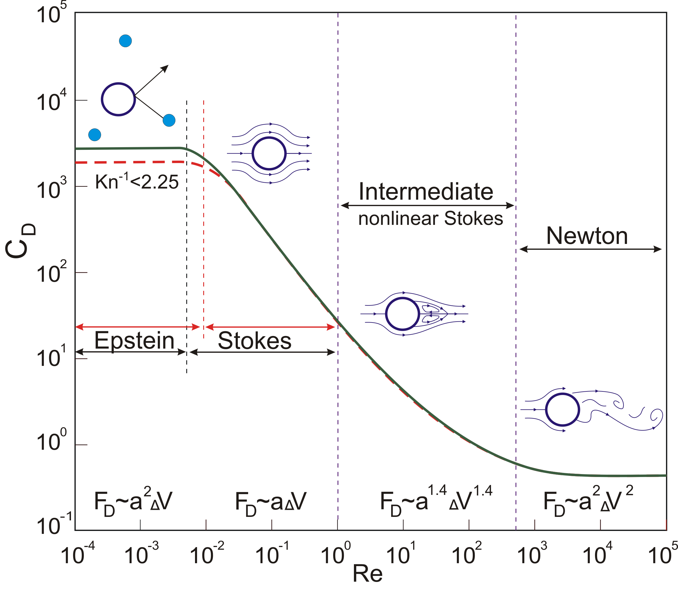
Figure 1: Drag coefficient as a function of the Reynolds and Mach numbers for the free-molecular flow regime (Epstein regime) and the case when the matter flows around a body like a continuous medium (the Stokes, transition, and Newton regimes). The boundary between free-molecular flow and continuous-medium flow is determined by the Knudsen number, and the boundaries of the continuous-medium flow regime by the Reynolds number. Stream lines around spherical particles are shown for the continuous-medium flow regimes. The functional dependence of the drag force $F_{\rm D}$ on the particle radius $a$ and relative velocity between the particles and gas $\Delta V=\|v-u\|$ are presented for all regimes.

In the case of a compressible gas, the drag coefficient $C_{\rm D}$ in (4) is a function of the two independent variables $\rm{Ma}$ and $\rm{Kn}$. The characteristic form of $C_{\rm D}$ is presented in Fig. 1. In a regime where the gas flows around the bodies like a continuous medium, the drag coefficient is determined by the Reynolds number $\rm{Re}$ (see, for example, [4]), which is derived from $\rm{Ma}$ and $\rm{Kn}$:

$$\rm{Re}=4\frac{\rm{Ma}}{\rm Kn}.$$ (7)

Particles with radii less than $2.25\lambda$, interact with the gas in a free-molecular-flow regime, or Epstein regime [15]. The drag coefficients for such bodies do not depend on $\rm{Re}$, but do depend on $\rm{Ma}$. This dependence corresponds to the standard astrophysical coefficient proposed in [46]:

$$C_{\rm D}=\left\{\begin{array}[]{lcl}\displaystyle\frac{8}{3}\rm{Ma}^{-1},\quad\rm{Kn^{-1}}<\frac{9}{4}\quad\textrm{(Epstein regime; I),}\\[10.0pt] \displaystyle 24\rm{Re}^{-1},\quad\rm{Re}<1\quad\textrm{(Stokes regime; II),}\\[10.0pt] \displaystyle 24\rm{Re}^{-0.6},\quad 1<\rm{Re}<800\quad\textrm{(transition regime or non-linear Stokes regime; III),}\\[10.0pt] \displaystyle 0.44,\quad\rm{Re}>800\quad\textrm{(Newton regime; IV).}\end{array}\right.$$ (8)

An approximation for the Stokes regime, the transition regime (also known as the non-linear Stokes regime), and the Newton regime in (8) was proposed in [32], and was applied in [47] to the aerodynamics of solid bodies in a disk. This approximation was expanded to encompass the Epstein regime in [46]. The coefficient (8) is used in [33, 23] and other studies in the framework of modern models for circumstellar disks.

Figure 2: Regions of determination of the piecewise function $C_{\rm D}$ (8), corresponding to the various flow regimes. I—Epstein, II—Stokes, III—transition (non-linear Stokes), IV—Newton. The green arrows indicate the boundaries at which a function is continuous, and the red x’s boundaries where a function is discontinuous.

Figure 2 presents the regions I–IV within which the drag coefficient $C_{\rm D}$ (as a function of $\rm{Kn^{-1}}$ and $\rm{Ma}$) is continuously differentiable. At the boundaries I–II, II–III, and III–IV, $C_{\rm D}$ is continuous, whereas this coefficient is discontinuous at the boundaries I–III and I–IV. The presence of a discontinuity is a serious inadequacy for simulations, since this can lead to the appearance of artificial singularities in the solution. We convinced ourselves that the conditions for which a particle makes the transition from the Epstein regime I to the transition regime (non-linear Stokes regime) III, which is accompanied by a discontinuity of the coefficient of friction (8). is indeed realized in simulations of the dynamics of a disk. This conclusion was based on the simulations of the dynamics of a viscous, self-gravitating, gaseous disk with a dust component using the FEOSAD model, which is described in detail in [43]. The disk model used differs from the basic model presented in [43]in the additional consideration of the influence of the dust dynamics on the gas dynamics, and also in the absence of the restriction on the size of the dust $a<2.25\lambda$, which artificially maintains the particles in the Epstein regime. We used drag coefficient (8) and the numerical scheme from Section 3.2 for our simulations. We used a constant value for the Shakura–Syunyaev viscosity over the disk, $\alpha=10^{-4}$, and the fragmentation velocity $v_{\rm frag}=30$ m s^-1. This Shakura–Syunyaev viscosity corresponds to a disk with suppressed magnetorotational instability, in which the transport of mass and angular momentum occurs mainly via gravitational torques in a non-axially symmetric disk. A fragmentation velocity $v_{\rm frag}$ determines the maximum particle size. The fragmentation velocity chosen corresponds to an enhanced probability of adhesion, as is realized when the particles are covered in a thick layer of ice.

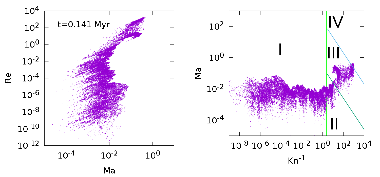
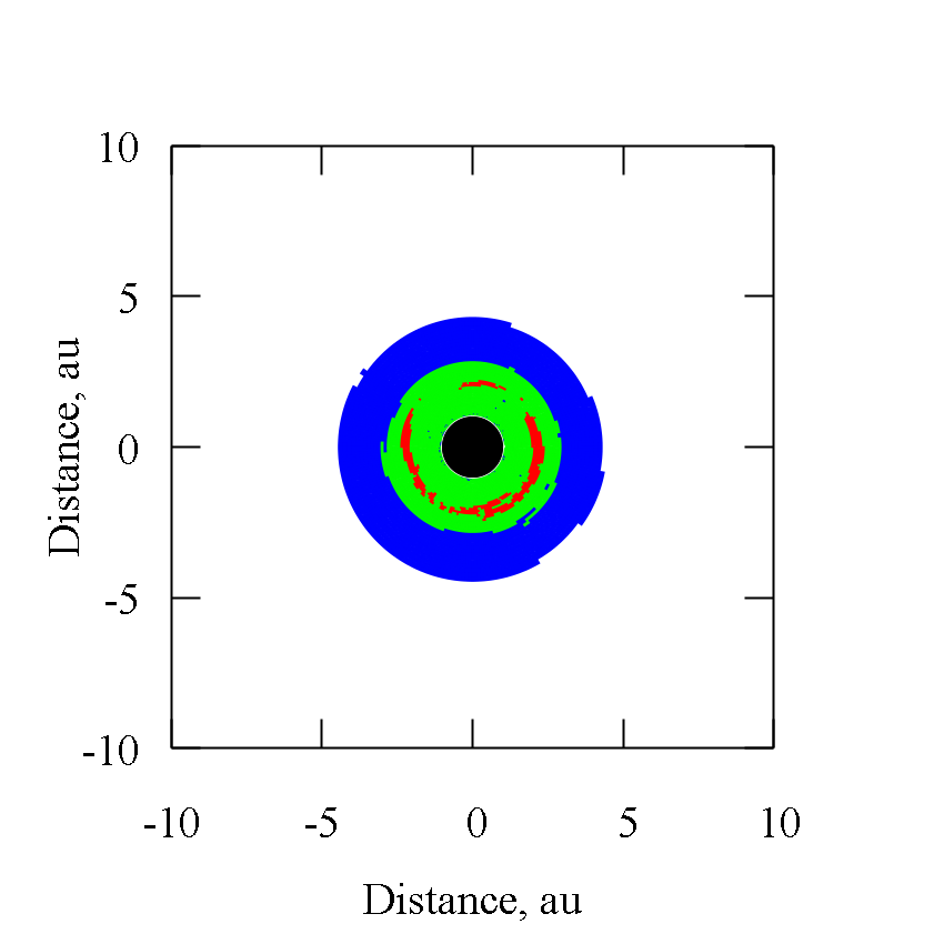
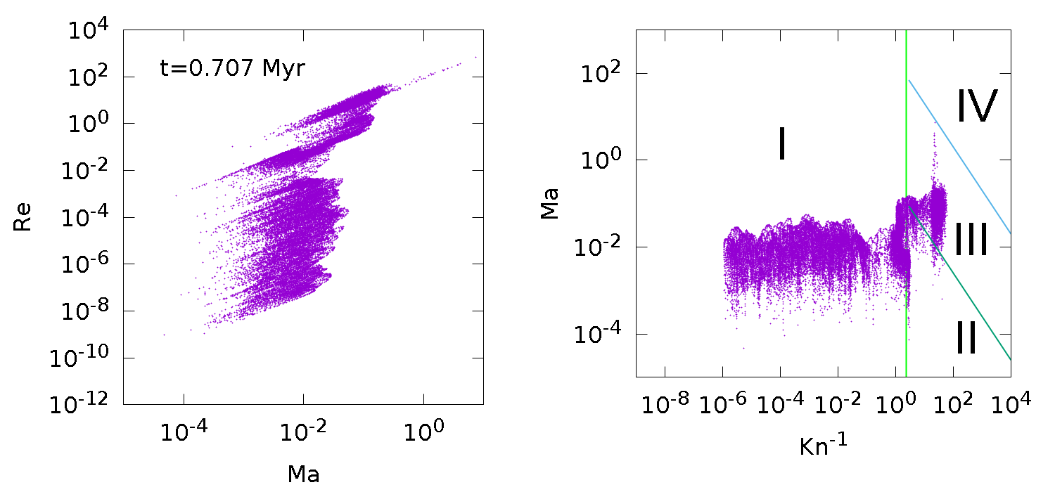
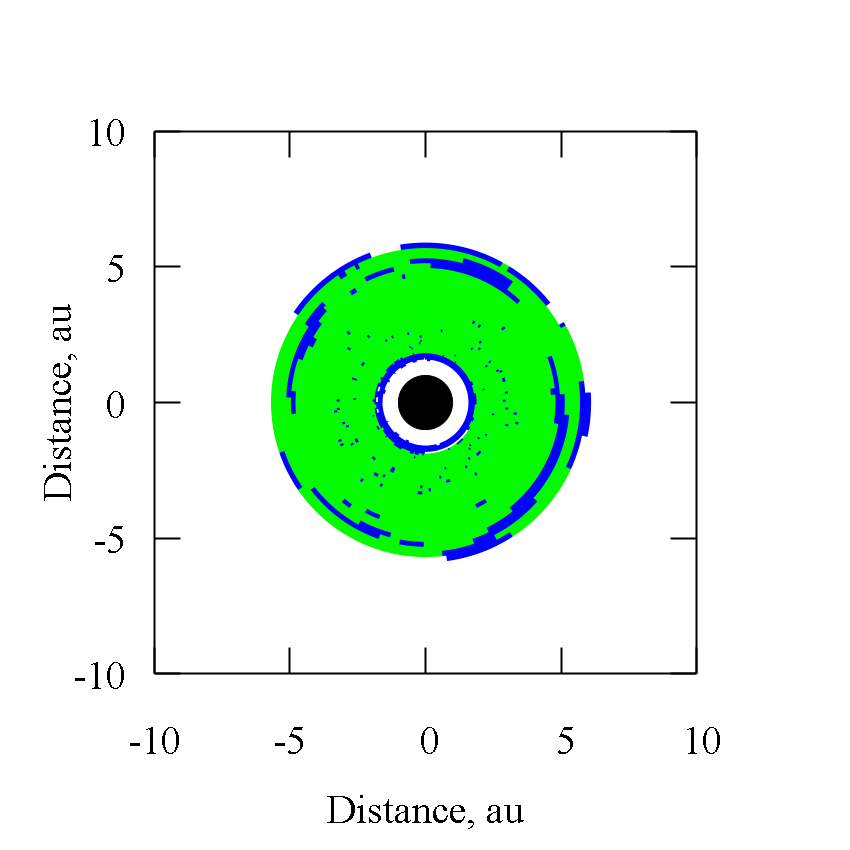
Figure 3: Values of $\rm{Ma}$ and $\rm{Re}$ (left column) and of $\rm{Ma}$ and $\rm{Kn}^{-1}$ (central column) for dust grains in all cells of circumstellar disks with ages of 141 000 years (upper row) and 707000 years (lower row). The various drag regimes from (8) are shown in the central panels by Roman numerals and in the right panels by different colors. I—Epstein (white), II—Stokes (blue), III—transition (non-linear Stokes) (green), IV—Newton (red). Black indicates drag cells of the disk. The standard astrophysical drag coefficient (8) is discontinuous at the boundary between the white and green region.

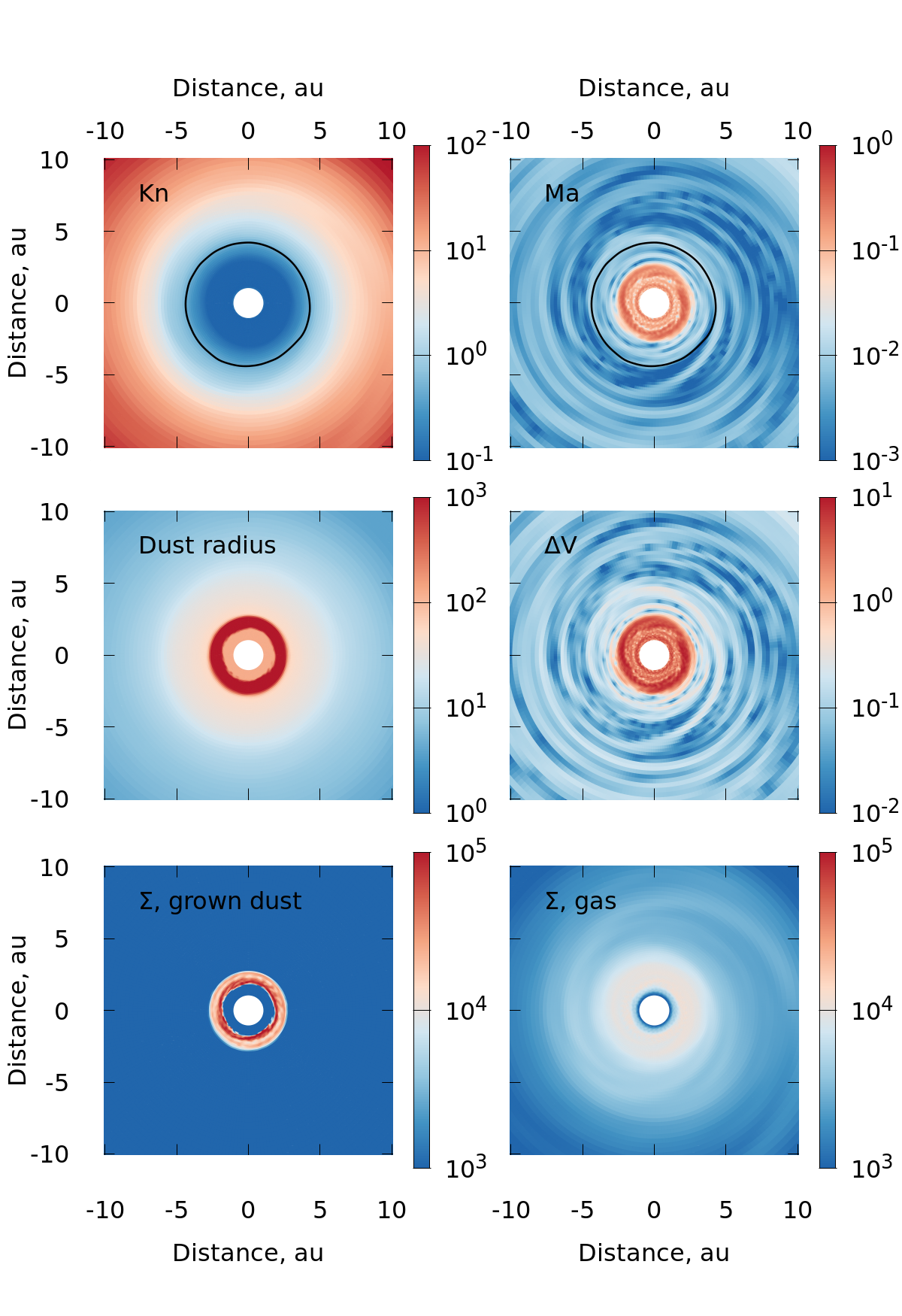
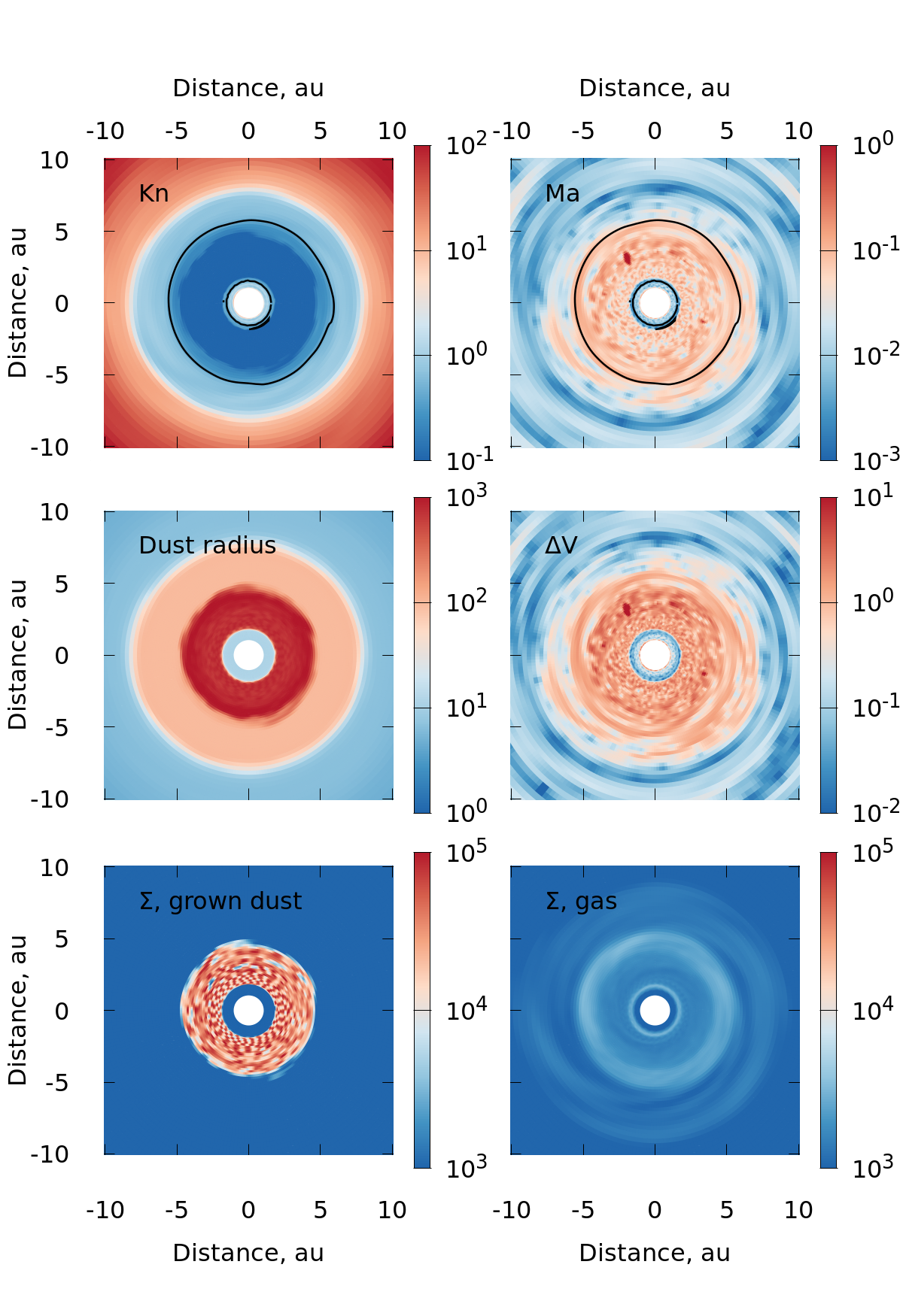
Figure 4: Distributions of physical quantities determining the drag regimes in the central regions of circumstellar disks with ages of 141000 years (left six panels) and 707000 years (right six panels). The upper panels present the Knudsen and Mach numbers and the lower panels present the surface densities of gas and grown dust in g cm^-2, The central panels show the maximum grain size $a$ in cm and the relative velocity between the gas and dust $\Delta V$ in km s^-1. The black contours in the upper panels show the boundary at which $a=4\lambda/9$. For a disk with an age of 141000 years, this passes through the region $\rm{Ma}\approx 0.01$, providing a continuous drag coefficient, while it passes through the region $\rm{Ma}\approx 1/9$, leading to a discontinuous drag coefficient for a disk with an age of 707000 years.

We computed the quantities $\rm{Kn}$, $\rm{Ma}$ and $\rm{Re}$ in each computational cell for the evolution of the disk over one million years. Figure 3 presents the set of values of these quantities in the disk in the $\rm{Ma}$, $\rm{Re}$ (left panels) and $\rm{Kn}^{-1}$, $\rm{Ma}$ (central panels) axis for ages of 141000 and 707000 years. The central panels show that the dust and gas interact in the free-molecular flow Epstein regime in the most part of the disk, however all four of the drag regimes indicated in (8) are realized in the disk. At a time of 707000 years (central panel in the second row), particles are present in the disk at the boundary of regions I–III, where the drag coefficient (8) undergoes a discontinuity. The right lower panel in Fig.3 where different colours indicate different regions in the disk with different drag regimes, shows that this discontinuity occurs at a distance of 6 au from the star. The distribution of physical quantities determining the drag regime in the central region of the circumstellar disk at the same times are shown in Fig. 4. The black contour in the upper panels, which present the Knudsen and Mach numbers, shows the boundary where $a=4\lambda/9$. In a disk with an age of 141000 years, this boundary passes through the region $\rm{Ma}\approx 0.01$, corresponding to a continuous coefficient of friction, while it passes through the region $\rm{Ma}\approx 1/9$ in a disk with an age of 707000 years, indicating the presence of a discontinuity in the drag coefficient.

Therefore, we investigated an alternative drag coefficient for cases when the medium flowing around the particles is compressible—the coefficient of Henderson [17]. The approximation of Henderson provides a good description of known experimental dependences for $\rm{Re}<3\times 10^{5}$ and $\rm{Ma}<6$(details can be found in [17] and references therein). It takes into account the difference between the gas and particle temperatures. For subsonic flow regimes (${\rm Ma}\leq 1$)

$$C_{\rm D}=\displaystyle\frac{24}{\mathrm{Re}+S\left(4.33+\displaystyle\frac{3.65-1.53T_{\rm d}/T_{\rm g}}{1+0.353T_{\rm d}/T_{\rm g}}\exp(-0.247\frac{\rm{Re}}{S})\right)}+0.6S\left(1-\exp\left(-\displaystyle\frac{\rm Ma}{\rm Re}\right)\right)$$ (9)

$$+\exp\left(-0.5\displaystyle\frac{\rm Ma}{\sqrt{\rm Re}}\right)\left(\displaystyle\frac{4.5+0.38\left(0.03{\rm Re}+0.48\sqrt{\rm Re}\right)}{1+0.03{\rm Re}+0.48\sqrt{\rm Re}}+0.1{\rm Ma}^{2}+0.2{\rm Ma}^{8}\right)$$ (10)

while for supersonic regimes (${\rm Ma}\geq 1.75$)

$$C_{\rm D}=\displaystyle\frac{0.9+\displaystyle\frac{0.34}{\rm{Ma}^{2}}+1.86\sqrt{\displaystyle\frac{\rm Ma}{\rm Re}}\left(2+\displaystyle\frac{2}{S^{2}}+\displaystyle\frac{1.058}{S}\sqrt{\frac{T_{\rm d}}{T_{\rm g}}}-\displaystyle\frac{1}{S^{4}}\right)}{1+1.86\displaystyle\sqrt{\frac{\rm Ma}{\rm Re}}},$$ (11)

where

$$S=\rm{Ma}\displaystyle\sqrt{\frac{\gamma}{2}},$$ (12)

$T_{\rm d}/T_{\rm g}$ is the ratio of the dust and gas temperatures. Intermediate values for the drag coefficient (when $1<\rm{Ma}<1.75$) can be obtained using a linear interpolation:

$$C_{\rm D}=C_{\rm D}({\rm Ma=1})+\displaystyle\frac{4}{3}(\mathrm{Ma}-1)\left(C_{\rm D}({\rm Ma=1.75})-C_{\rm D}({\rm Ma=1})\right),$$ (13)

where $C_{\rm D}({\rm Ma=1})$ can be found from (10), by substituting $\rm{Ma}=1$, and $C_{\rm D}({\rm Ma=1.75})$ can be found from (11), by substituting $\rm{Ma}=1.75$. Here and below, we assume $\gamma=1.4$, $T_{\rm d}/T_{\rm g}=1$.

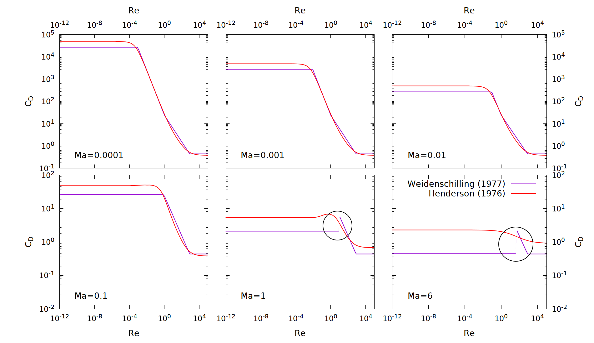
Figure 5: Henderson drag coefficient (10)-(13) and the standard astrophysical expression (8) for various $\rm{Ma}$ as a function of $\rm{Re}$.

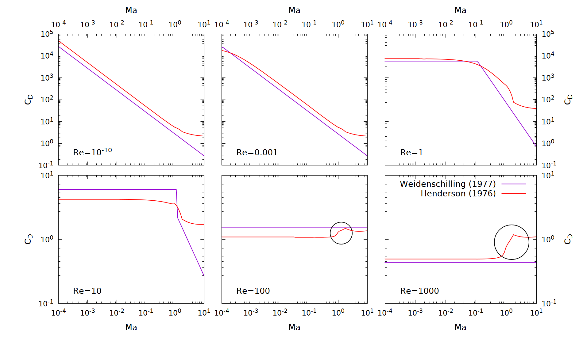
Figure 6: Henderson drag coefficient (10)–(13) and the standard astrophysical expression (8) for various $\rm{Re}$ as a function of $\rm{Ma}$.

The values of the standard astrophysical coefficient (8) and the Henderson coefficient (10)–(13) for the range of parameters of a circumstellar disk $10^{-4}\leq\rm{Ma}\leq 100$, $10^{-12}\leq\rm{Re}\leq 10^{3}$ are presented in Figs.5 and 6. It follows from the upper row of panels in Fig. 5 that both coefficients are similar when $\rm{Ma}\leq 0.01$ for any value of $\rm{Re}$. This is confirmed by the upper panels of Fig. 6. The values of the two drag coefficients differ quantitatively when $0.1\leq\rm{Ma}\leq 1$ and qualitatively when $\rm{Ma}\geq 1$. First, a discontinuity of the first type is visible in the standard astrophysical coefficient in the central and right panels of the lower row of Fig. 5. Furthermore, the lower right panel shows that the Henderson coefficient falls with growth in $\rm{Re}$, while the standard astrophysical coefficient grows. Second, the central and right panels of the lower row in Fig. 6 show that the Henderson coefficient has a feature (a bump near $\rm{Ma}=1$, well known in aeromechanics), which is absent in the simpler astrophysical approximation for the coefficient.

Thus, when simulating the dynamics of a gas–dust medium with $\rm{Ma}>1/9$, it is recommended to use only the Henderson coefficient. However, if the treatment is restricted to $\rm{Ma}\leq 1/9$, the standard astrophysical coefficient is less computationally expensive and convenient for programming.

3 NUMERICAL METHODS FOR SOLVING THE EQUATIONS OF MOTION OF A GAS-DUST MEDIUM WITH INTENSE INTER-PHASE INTERACTIONS

3.1 Review of Earlier Studies

We define the time scale for the velocity of a spherically symmetrical particle to relax to the velocity of the ambient gas as follows:

$$t_{\rm stop}=\frac{m_{\rm p}\|v-u\|}{\|F_{\rm D}\|}=\frac{\frac{4}{3}\pi a^{3}\rho_{\rm s}\|v-u\|}{\frac{1}{2}C_{\rm D}\pi a^{2}\rho_{\rm g}\|v-u\|^{2}}=\frac{8}{3}\frac{a\rho_{\rm s}}{C_{\rm D}\rho_{\rm g}\|v-u\|},$$ (14)

where $m_{\rm p}$ is the mass of the particle and $\rho_{\rm s}$ is the material density of the grains.

For dust grains with sizes of about one micron in an orbit with a radius of 100 au, the estimated relaxation, or stopping, time $t_{\rm stop}$ in the disk is of order 100 s (see, for example, [40, 22]), while the disk dynamics require simulations over $10^{4}$ yrs $\approx 10^{11}$ s or more. This means that the equations of motion of the gas and dust have stiff relaxation terms associated with intense interphase interactions. This makes simulations the dynamics of gas–dust disks a challenging task in modern computational astrophysics (see, for example, [16]).

Problems with stiff relaxation terms have been actively studied in applied mathematics [11]. In addition to the dynamics of multiphase media, such problems also arise in plasma physics, models for elasticity with memory, problems in kinetic theory, and so forth. When explicit methods are used to obtain stable numerical solutions, the time step must satisfy the condition $\tau\leq t_{\rm stop}$, which is unacceptably expensive for simulations of multi-physics systems of equations in the two-dimensional and three-dimensional cases, even on modern supercomputers.

In particular, when modeling the dynamics of a gaseous, self-gravitating disk (e.g., [42, 39]), the time step indicated by the Courant condition is several Earth days. When necessary, this step can be made up to a factor of 100 shorter, but the time for the solutions to be obtained then increases by a factor of 100–1000, making it infeasible to carry out series of computational experiments.

There is no restriction on the time step from the stability point of view when using implicit methods, but restrictions can arise due to the required accuracy [31]. For example, in an early study, Jim and Livermore [20] showed that, in general, in the presence of stiff relaxation terms, even high-accuracy grid methods can reproduce asymptotic behavior of the solutions only if a very small spatial step is used. Examples of the manifestation of such effects in simulations of the dynamics of circumstellar disks can be found in [40, 43, 23]. In particular, the diffusion overdissipation of solutions obtained in simulations of the dynamics of a gas–dust medium using smoothed particle hydrodynamics (SPH) with computations of the interphase interactions using a classical approach [29] were studied in [24, 23]. An empirical criterion was derived, according to which the overdissipation of the solutions is at an acceptable level if the smoothing radius $h<c_{\rm s}t_{\rm stop}$ is used. According to this criterion, simulations of the dynamics of micron-sized particles in a circumstellar disk requires a spatial resolution $h\approx 10$ km, whereas the radius of the disk is of order $10^{10}$ km. It is clear that such a spatial resolution is beyond the capabilities of modern computational technology.

In a number of cases, a search for a numerical solution of a stiff problem can be substituted with the solution to a simpler problem obtained from the original one via expansion in a small parameter (this general idea is presented in [11], and its application to simulations of a gas–dust medium in a circumstellar disk in [21, 1, 2], for example). The simplified problem becomes non-stiff, but this approach is justified only if the relaxation time is much smaller than the time scale for the motion of the carrier phase, and it cannot be used to model the transition regime when the relaxation time is close to the dynamical time scale. Moreover, this approach may involve a change in the type of equations considered.

Therefore, an alternative to adopting a simplified problem is the development of implicit and semiimplicit numerical methods that are able to precisely reproduce the equilibrium values, even with crude spatial resolution. Attempts are currently being made to find a general approach to the construction of highaccuracy methods for problems with relaxation terms (see, e.g., [3]). However, in most studies of the numerical solution of such systems, the methods are constructed taking into account the specifics of the problem to be solved and specific forms for the “stiff relaxation term”. In particular, when simulating the dynamics of a gas–dust medium, the system has not one, but two stiff relaxation terms—in the equations of motion for the gas and dust [27, 24, 19, 48]). On average over the disk, $\varepsilon=\displaystyle\frac{\rho_{\rm d}}{\rho_{\rm g}}$ is equal to 0.01, to order of magnitude, so that the influence of the dust on the gas dynamics can often be neglected. On the other hand, the results of simulations indicate that the dust particles may be concentrated in specific regions of the disk (e.g., in spiral arms [33], in the inner part of the disk [43], in self-gravitating gaseous clumps [10]), increasing the density ratios in these locations to values $\varepsilon\approx 1$ or more.

Several groups of researchers are currently working on creating numerical models for the dynamics of a gas–dust medium with a high concentration of the dispersed phase and intense interphase interactions, based on grid methods and SPH.

Benitez-Llambay et al. [7] presented a non-iterative implicit grid method and set of test problems for a medium of gas and polydisperse dust in a circumstellar disk. In their model, each fraction of the polydisperse dust exchanges momentum with gas, but there is no energy exchange between the gas and dust. They showed that their proposed method is stable, has low dissipative properties, and preserves the asymptotic behaviour of the solution for any time step.

Sadin [41] and Sadin and Odoev [34] proposed a finite-difference scheme with customizable dissipative properties aimed at simulating the dynamics of a medium of gas and monodisperse dust.

A non-iterative, implicit method based on SPH for monodispersive and polydisperse dust is presented in [25, 23, 18]. This model for the dynamics of the gas– dust medium is based on a one-fluid approach (the equations for the properties of the gas–dust medium as a whole are solved, solving the diffusion equation for the concentration of the solid phase). In this approach, each SPH particle carries the features of both the gas and the dust. This approach is fast, and free of the numerical dissipation that arises in the application of Lagrangian methods in a two-fluid approach. On the other hand, the conservation of mass for the dispersed phase is not guaranteed in a one-fluid approach. In addition, there is a stricter bound from above on the size of the dispersed phase particles, compared to the two-fluid approach.

Lóren-Aguilar and Bate [27, 28] developed a twofluid approach based on SPH for a medium of gas and monodispersive dust. They found that the numerical overdissipation in the gas–dust medium was smaller in their solutions than in the classical SPH approach [29]. However, this dissipation was higher than the diffusion dissipation in the gas due to artificial viscosity.

Stoyanovskaya et al. [38] proposed a new method for solving the motion equations of gas and monodisperse dust with intense interphase interactions based on SPH. Their proposed method for computing the interphase interactions is non-iterative and has low dissipative properties. These features of the method are determined by the implicit linear approximation for the drag force used, together with the local conservation of momentum in the computations of the drag between the gas and dust.

All these developments were made for the most common regime for the interactions between particles and gas in a circumstellar disk—the Epstein regime. In this regime, there are intense interphase interactions, and drag term depends linearly on the relative velocity between the gas and particles. However, the simulation results show that grown solids interact with the gas in a transition and Newton regimes, when the interphase interactions are moderate and the drag depends non-linearly on the relative velocity between the gas and particles. Accordingly, in our current study, we propose a scheme for the time discretization of the equations of motion of the gas and dust that encompasses both cases and can be used with any method for computing the spatial derivatives if the velocities of the gas and dust are determined at the same points in space. This method for the simulation of the dynamics of a medium of gas and dust with drag that depends linearly on the relative velocity between the gas and dust is a special case of the approach of [7], which is well justified in the linear case. Thus, our study can be considered as a basis for the approach to the simulation of polydisperse dust [7] with a transition from linear to non-linear drag.

3.2 Fast and Asymptotic Preserving Scheme for the Time Discretization of the Equations of Motion of the Gas and Dust

To approximate the interphase interactions in the equations of motion in (1)-(2), we linearized the drag term on the relative velocity between the gas and particles, with the stopping time $t_{\rm stop}(\rho_{\rm g},u-v)$ computed using known quantities from the previous step and the relative velocity of the gas and particles computed from the subsequent step. A simple description of this approach has the form:

$$\frac{v^{n+1}-v^{n}}{\tau}+(v^{n}\cdot\nabla)v^{n}=-\displaystyle\frac{\nabla p^{n}}{\rho_{\rm g}^{n}}+g^{n}-\frac{\rho^{n}_{\rm d}}{\rho^{n}_{\rm g}}\frac{v^{n+1}-u^{n+1}}{t^{n}_{\rm stop}}+\frac{f^{n}_{\rm g}}{\rho_{\rm g}^{n}},$$ (15)

$$\frac{u^{n+1}-u^{n}}{\tau}+(u^{n}\cdot\nabla)u^{n}=g^{n}+\frac{v^{n+1}-u^{n+1}}{t^{n}_{\rm stop}}+\frac{f^{n}_{\rm d}}{\rho_{\rm d}^{n}}.$$ (16)

We solved the entire system (1)-(2) using a two-stage scheme based on the operator splitting method with respect to physical processes (as in our earlier studies [40, 37]). We solved the continuity equation and the equation of motion using the finite-difference method described in detail for a pure gas in [36]. In the first stage of the scheme, the advective terms and transport of mass and momentum are computed:

$$\frac{\partial\rho_{\rm g}}{\partial t}+\nabla(\rho_{\rm g}v)=0,\ \ \ \rho_{\rm g}\left[\displaystyle\frac{\partial v}{\partial t}+(v\cdot\nabla)v\right]=0,$$ (17)

$$\frac{\partial\rho_{\rm d}}{\partial t}+\nabla(\rho_{\rm d}u)=0,\ \ \ \rho_{\rm d}\left[\displaystyle\frac{\partial u}{\partial t}+(u\cdot\nabla)u\right]=0.$$ (18)

We computed the spatial derivatives in each stage using the piecewise-parabolic method of [12]. In this stage, we determined the quantities $\rho_{\rm g}^{n+1/2}$, $\rho_{\rm d}^{n+1/2}$, $v^{n+1/2}$, $u^{n+1/2}$.

In the next stage, we computed the influence of the forces of pressure, drag, gravitation, and other effects using the updated densities and velocities of the gas from the first stage:

$$\frac{v^{n+1}-v^{n+1/2}}{\tau}=-\displaystyle\frac{\nabla p^{n+1/2}}{\rho_{\rm g}^{n+1/2}}+g^{n+1/2}-\frac{\rho^{n+1/2}_{\rm d}}{\rho^{n+1/2}_{\rm g}}\frac{v^{n+1}-u^{n+1}}{t^{n+1/2}_{\rm stop}}+\frac{f^{n+1/2}_{\rm g}}{\rho_{\rm g}^{n+1/2}},$$ (19)

$$\frac{u^{n+1}-u^{n+1/2}}{\tau}=g^{n+1/2}+\frac{v^{n+1}-u^{n+1}}{t^{n+1/2}_{\rm stop}}+\frac{f^{n+1/2}_{\rm d}}{\rho_{\rm d}^{n+1/2}}.$$ (20)

Thanks to the fact that $v^{n+1}$ and $u^{n+1}$ can be expressed explicitly using (15), (16), the computational costs required for the semi-implicit approximation of friction are similar to those for an explicit approximation.

3.3 Testing of the Scheme

In Section (3.3.1), we will consider the degree of numerical overdissipation of the scheme (15), (16) during the computation of intense interphase interaction using a time step $\tau$, determined by the Courant condition, and not $t_{\rm stop}$. In Section 3.3.2 we will compare the accuracy of solutions obtained using the firstorder scheme (15), (16) and a fourth-order scheme to simulate the motion of single dust grain in a gaseous disk whose angular velocity is slightly sub-Keplerian.

3.3.1 Test 1. Strong shocks in a gas–dust medium.

In the one-dimensional equations (1) and (2), we set $g=0$, $S_{\rm g}=S_{\rm d}=0$, $f_{\rm g}=f_{\rm d}=0$, $f_{\rm D}=\displaystyle\frac{\rho_{\rm d}(v-u)}{t_{\rm stop}}$ and wrote the energy equation:

$$\rho_{\rm g}\left(\frac{\partial e}{\partial t}+v\frac{\partial e}{\partial x}\right)=-p\frac{\partial v}{\partial x},$$ (21)

where $e$ is the internal energy of the gas, which is related to the pressure as

$$p=\rho_{\rm g}e(\gamma-1),$$ (22)

where $\gamma$ is the adiabatic index. We made this system dimensionless using the length $l_{*}$, mass $m_{*}$, and time $t_{*}$units, so that the derivative dimensional quantities have the form $\rho_{*}=\displaystyle\frac{m_{*}}{l_{*}^{3}}$, $v_{*}=\displaystyle\frac{l_{*}}{t_{*}}$, $p_{*}=\displaystyle\frac{m_{*}}{t_{*}^{2}l_{*}}$, $e_{*}=\displaystyle\frac{l_{*}^{2}}{t_{*}^{2}}$. We solved the system in the dimensionless variables.

For the resulting system (1), (2), (21), (22), we specified a no-flow condition at the boundaries of an interval. We specified the velocities to be zero at the initial time, and specified the jumps in the gas pressure and in the densities of the gas and dust to be

$$\left[\displaystyle\frac{\rho_{\rm{g}}}{\rho_{*}},\frac{p}{p_{*}},\frac{e}{e_{*}},\frac{\rho_{\rm{d}}}{\rho_{*}}\right]_{\it l}=[1,1,2.5,1],$$

$$\left[\displaystyle\frac{\rho_{\rm{g}}}{\rho_{*}},\frac{p}{p_{*}},\frac{e}{e_{*}},\frac{\rho_{\rm{d}}}{\rho_{*}}\right]_{\it r}=[0.125,0.1,2,0.125],$$

$$\gamma_{l}=\gamma_{r}=7/5.$$

We specified $\lambda=\displaystyle 5\cdot 10^{-6}l_{*}\frac{\rho_{*}}{\rho_{\rm g}}$, $\rho_{\rm s}=2.3\rho_{*}$ and considered two particle sizes: small grains with $a=5\cdot 10^{-6}l_{*}$ and large grains with $a=10^{-2}l_{*}$.

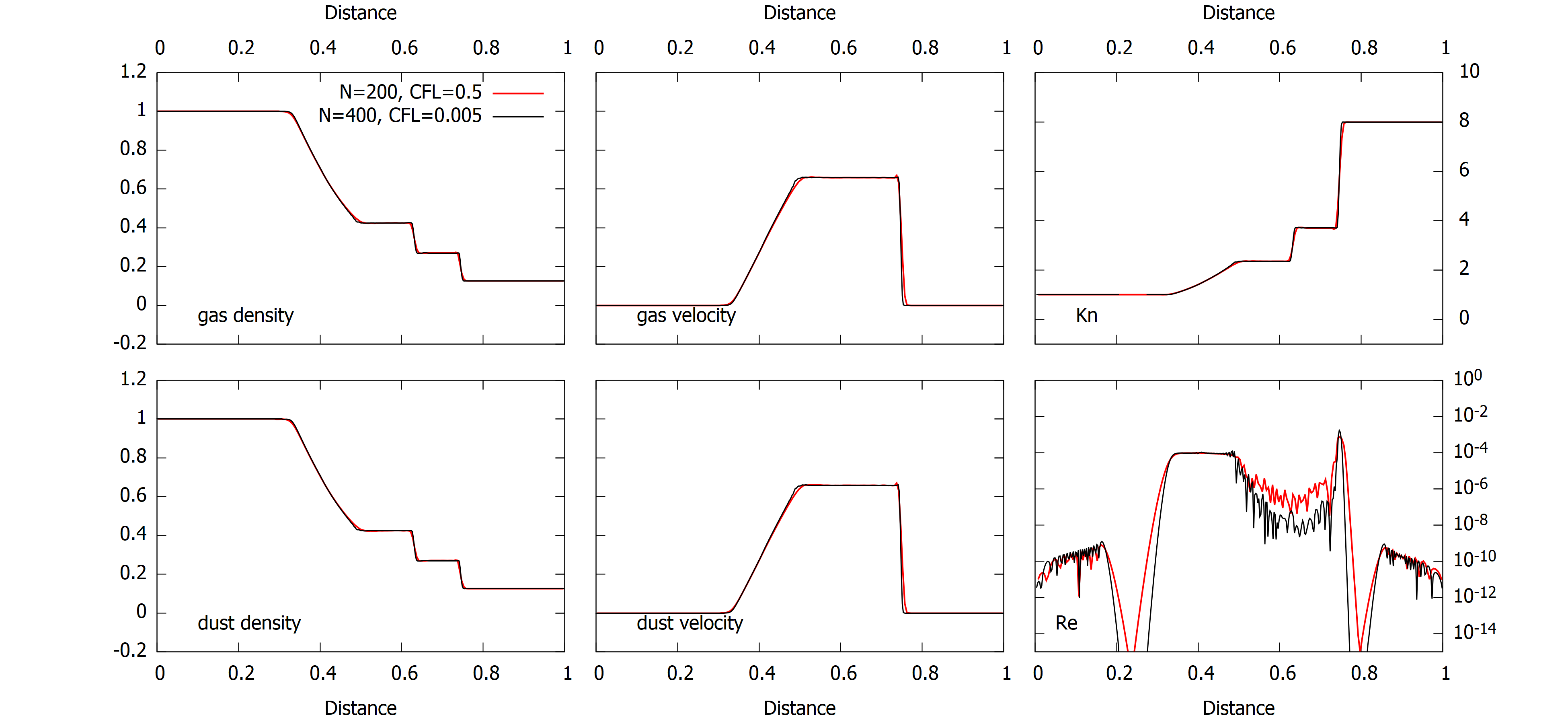
Figure 7: Solution for a Sod shock tube for the scheme (15), (16), which preserves the asymptotic behavior, for $\rm{Kn}\geq 1$ (small dust with $a=5\cdot 10^{-6}l_{*}$, the Epstein regime, Henderson drag coefficient (10)–(13)).

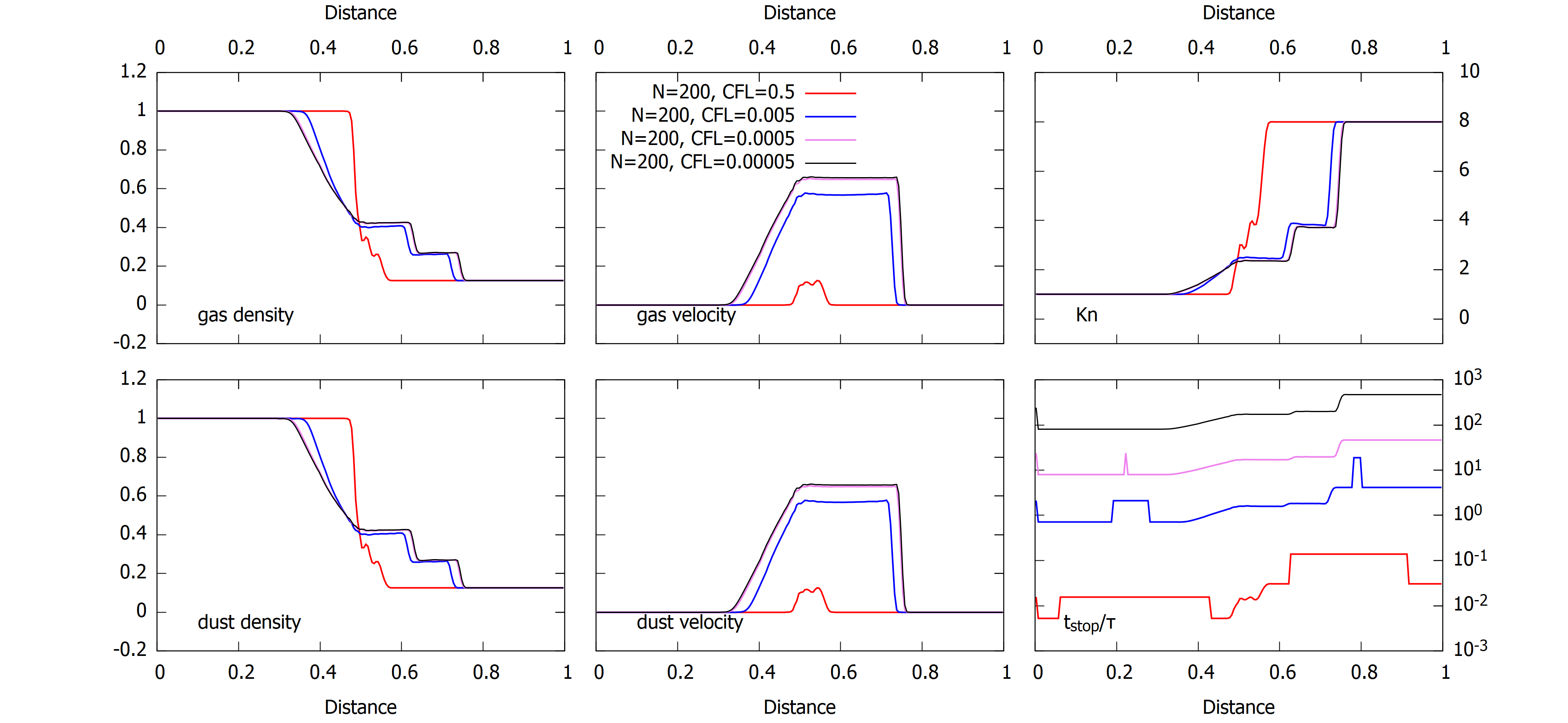
Figure 8: Solution for a Sod shock tube for the scheme (23), (24), which does not preserve the asymptotic behavior, with various time steps for $\rm{Kn}\geq 1$ (small dust with $a=5\cdot 10^{-6}l_{*}$, Epstein regime, Henderson drag coefficient (10)–(13)).

It was shown in [40] that the semi-implicit, first-order operator splitting scheme (15), (16) preserves the asymptotic solutions in computations of intense interphase interactions with a constant drag coefficient. This same conclusion follows from Fig.. 7 for the case when $C_{\rm D}$ varies in space and time and $t_{\rm stop}=t_{\rm stop}(\|u-v\|)$.

Figure 7 presents simulations with the Henderson drag coefficient (10)–(13) for a grain size $a=5\cdot 10^{-6}l_{*}$. We adopted the results for our simulations with detailed spatial resolution with $N=400$ cells per segment and a time step for which the Courant parameter is $\mathrm{CFL}=0.005$ as a reference. It is clear that the computations of the gas and dust velocities and densities with $N=200,\mathrm{CFL}=0.5$ differ only slightly from the reference results. In addition to computations with $\rho_{\rm d}/\rho_{\rm g}=1$, we also carried out simulations for the same problem with the dust content relative to the gas content enhanced by a factor of 10 and 1000. We confirmed that the level of numerical overdissipation of the solution remained insignificant for these cases in computations using the asymptotic-preserving scheme.

An example of a semi-implicit drag term approximation that does not preserve the asymptotic behavior is

$$\frac{v^{n+1}-v^{n}}{\tau}+(v^{n}\cdot\nabla)v^{n}=-\displaystyle\frac{\nabla p^{n}}{\rho_{\rm g}^{n}}+g^{n}-\frac{\rho^{n}_{\rm d}}{\rho^{n}_{\rm g}}\frac{v^{n+1}-u^{n}}{t^{n}_{\rm stop}}+\frac{f^{n}_{\rm g}}{\rho_{\rm g}^{n}},$$ (23)

$$\frac{u^{n+1}-u^{n}}{\tau}+(u^{n}\cdot\nabla)u^{n}=g^{n}+\frac{v^{n+1}-u^{n+1}}{t^{n}_{\rm stop}}+\frac{f^{n}_{\rm d}}{\rho_{\rm d}^{n}}.$$ (24)

The solution of this problem obtained using the scheme (23), (24) is presented in Fig. 8. This figure shows that, when $\mathrm{CFL}$ is varied from 0.5 to 0.00005, the computed wave-propagation speeds vary significantly, with the accuracy of the resulting solution being satisfactory only when $\tau<0.1t_{\rm stop}$.

It follows from the upper panel of Fig. 7 that the Knudsen number for the small grains exceeds unity. This means that, according to the regime classification (8), the interaction of the gas and dust occurs in the Epstein free-molecular-flow regime. The computation of $t_{\rm stop}^{n}$ was carried out using the general formula (14) for linear and non-linear drag term. Note that the influence of the numerical resolution on the results is visible only in the lower right panel of Fig. 7, which presents the quantity $\rm{Re}$, which depends linearly on $\|u-v\|$. It is known, however (see, e.g., [22]), that the relative velocity of the gas and dust can be ignored in the case $t_{\rm stop}\max(u,v)\ll l_{*}$, and the solution for a gas–dust medium can be obtained from the solution for a gaseous medium by replacing $c_{\rm s}$ by

$$c^{*}_{s}=c_{s}\left(1+\displaystyle\frac{\rho_{\rm d}}{\rho_{\rm g}}\right)^{-1/2}.$$ (25)

This means that the solution of the stationary problem does not depend on the drag coefficient and $t_{\rm stop}$, and is determined by the ratio of the dust and gas densities. Therefore, the appreciable deviations of $\rm{Re}$ for different spatial resolutions presented in the lower right panel of Fig. 7, do not lead to substantial differences in the quantities depicted in the other panels. This conclusion is supported by the right panels of Fig. 10, which show the velocities of the gas and dust obtained for small grains with $N=200$ and $\mathrm{CFL}=0.5$ and for various drag coefficients.

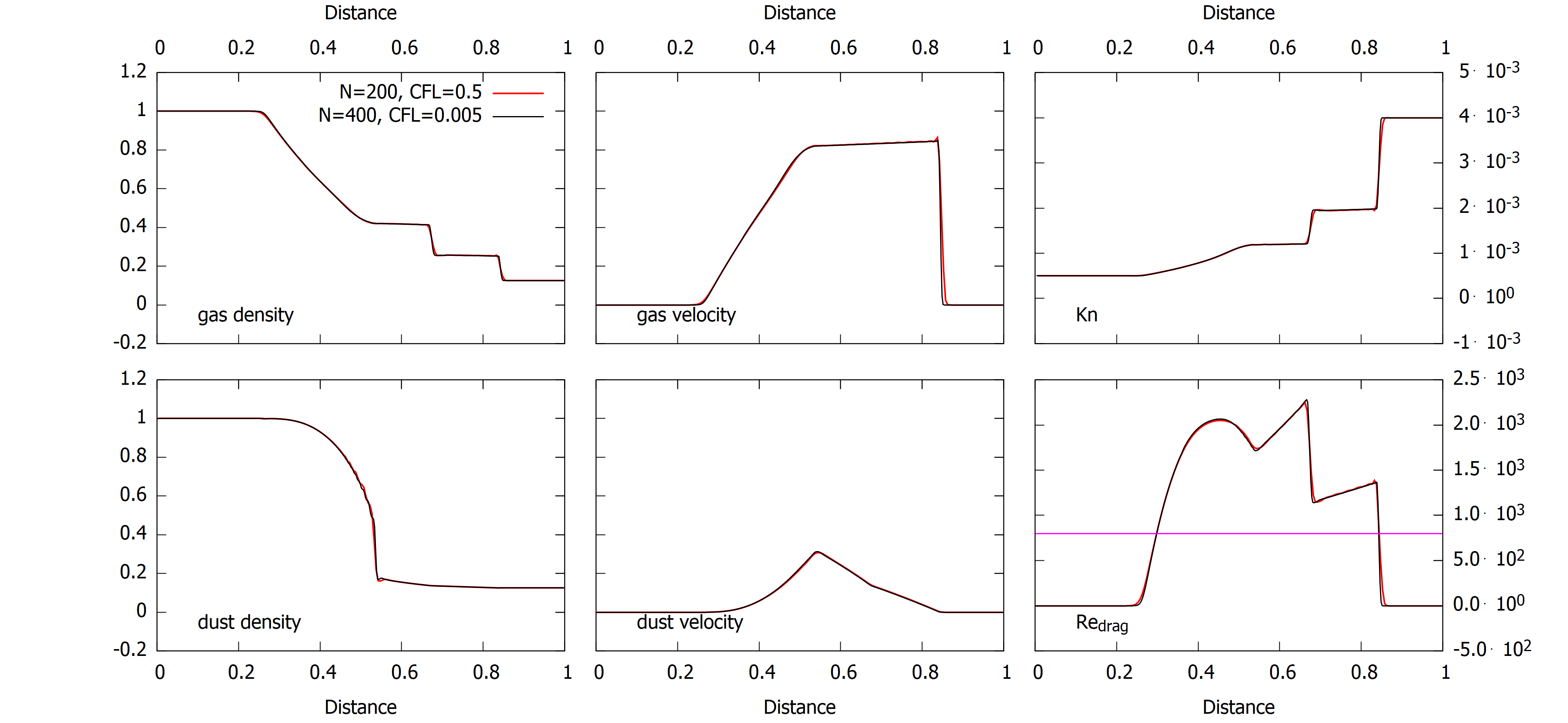
Figure 9: Solution for a Sod shock tube for the scheme (15), (16), which preserves the asymptotic behavior, with various steps in space and time, for $\rm{Kn}\ll 1$ (large bodies, the Stokes, transition, and Newton regimes, non-linear drag), Henderson drag coefficient (10)–(13)).

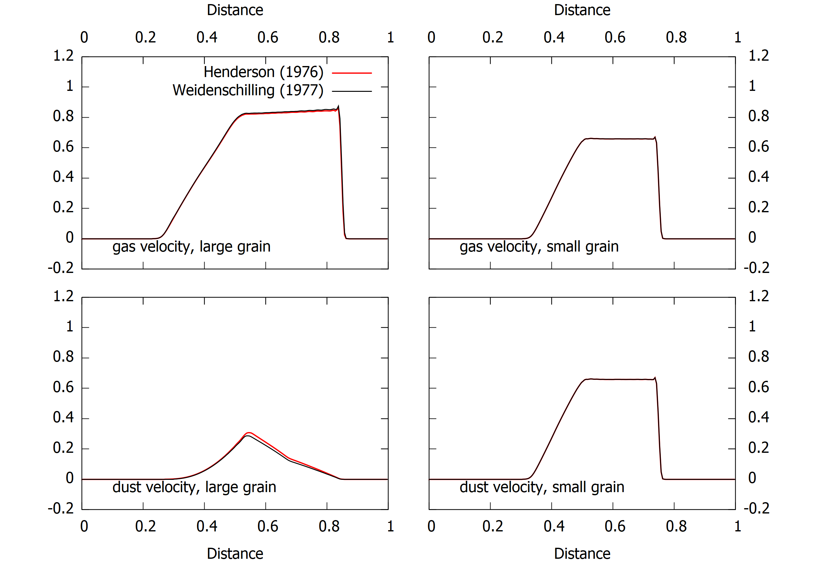
Figure 10: Solution for a Sod shock tube for large bodies (left panels) and small grains (right panels) with the Henderson (10)–(13) and standard astrophysical (8) drag coefficients.

The level of numerical overdissipation of the solution obtained using the scheme (15), (16) for the case of moderate interphase interactions can be seen in Fig. 9, which shows the same computational results as in Fig. 7 for an enhanced grain size of $a=10^{-2}l_{*}$. It follows from the right panels of Fig. 9 that, for the specified grain size, the gas flows around the particles like a continuous medium ($\rm{Kn}\ll 1$) with the Stokes regime, transition regime, and Newton regime being realized. The simulation results for $N=200,\mathrm{CFL}=0.5$ differ only insignificantly from the reference solution. In contrast to the regime with intense interphase interactions, the velocity and density distribution of the dust differ appreciably from those for the gas. In the left panels of Fig. 10, which show the velocities of the gas and dust, we can see a more clearly defined dependence of the solution on the drag coefficient for larger than for smaller grains.

Overall, the results presented show that the scheme (15), (16) preserves the asymptotic behavior of the solution in simulations with both intense and moderate interphase interactions.

3.3.2 Test 2. Simulation of a particle trajectory in a stationary circumstellar disk.

The equation of motion of a particle in the field of a massive central body in polar coordinates is presented, for example, in [26]. If gas drag acts on the particle together with gravitational and the centrifugal force, according to (4), these equations acquire the form:

$$\left\{\begin{array}[]{lcl}\displaystyle\frac{dr}{dt}=v_{r},\\ \displaystyle\frac{dv_{r}}{dt}=\frac{v_{\varphi}^{2}}{r}-\frac{GM}{r^{2}}-\frac{3}{8}\frac{C_{\rm D}\rho_{\rm g}(u_{r}-v_{r})||u-v||}{a\rho_{s}},\\ \displaystyle\frac{dv_{\varphi}}{dt}=-\frac{v_{r}v_{\varphi}}{r}-\frac{3}{8}\frac{C_{\rm D}\rho_{\rm g}(u_{\varphi}-v_{\varphi})||u-v||}{a\rho_{\rm s}},\end{array}\right.$$ (26)

where $r$ is the orbital radius of the particle, $(v_{r},v_{\varphi})$ the radial and azimuthal velocities of the particle, $(u_{r},u_{\varphi})$ the velocity of the gas, $M$ the mass of the central body, and $G$ the gravitational constant. We took the distributions of the density, temperature, and velocity in the axially symmetric gaseous disk to be given by the model [33] (a detailed description of the model is presented in the Appendix B), and to display the following dependences on the radius: $\rho_{\rm g}\sim r^{-2.25}$, $c_{s}\sim r^{-0.75}$, $u_{r}=0$. Let us supposed that the central body has a mass of $0.5$ $M_{\odot}$ and the disk extends from 1 au to 100 au and has a mass of $0.4$ $M_{\odot}$. Let the material density of solid bodies be $\rho_{\rm s}=2.2$ g cm ^-3.

At the initial time, we specified the particle to have an orbital radius $r_{0}=10$ au and a velocity $v_{\varphi 0}=0.25V_{\rm K}(r_{0})$, where $V_{\rm K}(r)=\displaystyle\sqrt{\frac{GM}{r}}$, $v_{r0}=-10^{-4}$ au$\cdot\Omega(r=1$ au), where $\Omega(r)=\displaystyle\frac{V_{\rm K}(r)}{r}$. We assumed that the size of particles drifting in the disk grows as $a=a_{0}\left(\displaystyle\frac{r}{r_{0}}\right)^{-3}$, with the particles a distance $r_{0}$ from the central body having sizes $a_{0}=134.64$ cm (Toy Model 1) or $a_{0}=13.464$ cm (Toy Model 2). We simulated the motion of a particle toward the central body until its orbital radius reached 1 au. We used the semi-implicit first-order scheme

$$\left\{\begin{array}[]{lcl}\displaystyle\frac{r^{n+1}-r^{n}}{\tau}=v^{n}_{r},\\ \displaystyle\frac{v^{n+1}_{r}-v^{n}_{r}}{\tau}=\frac{(v^{n}_{\varphi})^{2}}{r^{n}}-\frac{GM}{(r^{n})^{2}}-\frac{3}{8}\frac{C^{n}_{\rm D}\rho^{n}_{\rm g}(u^{n+1}_{r}-v^{n+1}_{r})||u^{n}-v^{n}||}{a^{n}\rho_{s}},\\ \displaystyle\frac{v^{n+1}_{\varphi}-v^{n}_{\varphi}}{\tau}=-\frac{v^{n}_{r}v^{n}_{\varphi}}{r^{n}}-\frac{3}{8}\frac{C^{n}_{\rm D}\rho^{n}_{\rm g}(u^{n+1}_{\varphi}-v^{n+1}_{\varphi})||u^{n}-v^{n}||}{a^{n}\rho_{\rm s}},\end{array}\right.$$ (27)

with a time step of $\tau=0.01\Omega^{-1}(r=1$ au). This value of $\tau$ means that a particle that moves with Keplerian velocity in a circular orbit of radius 1 au makes a full orbit in 628 steps. This time step will be obtained from the Courant condition when the dynamics of a gaseous disk is modeled in cylindrical coordinates with a resolution of 256 cells in azimuth and with Courant number $\mathrm{CFL}=0.4$.

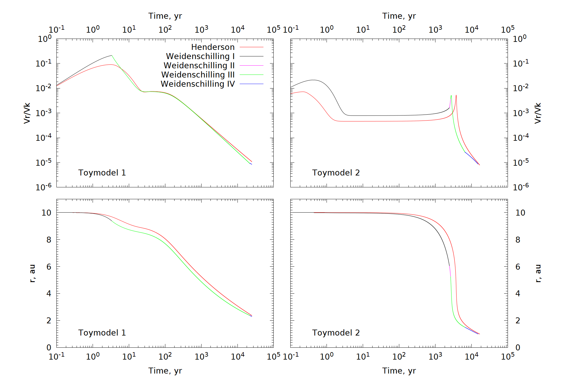
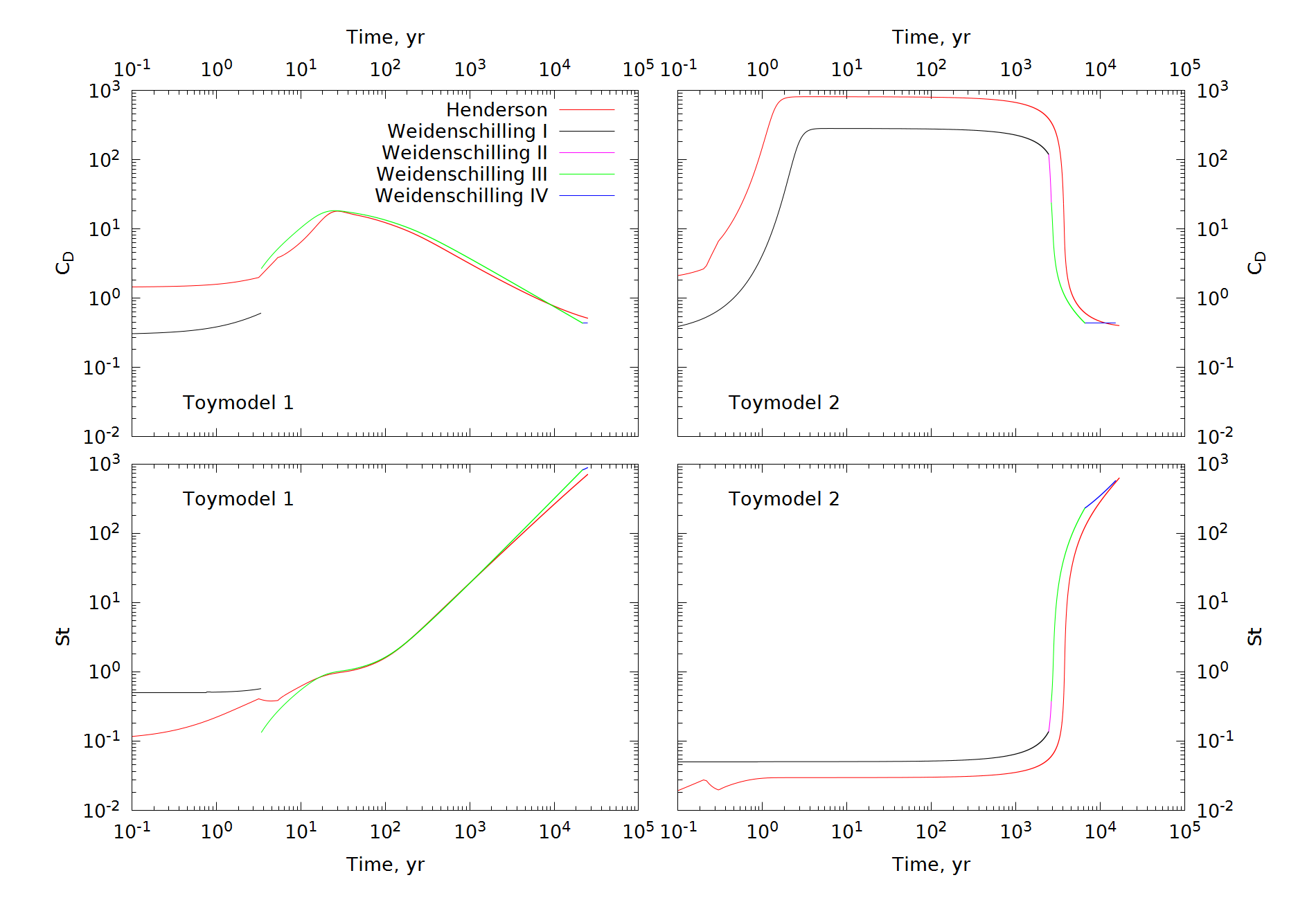
Figure 11: Simulations of the trajectory of a growing dust particle in a stationary gaseous disk with mass 0.4 $M_{\odot}$ around a central body with mass 0.5 $M_{\odot}$ with various drag coefficients. The red curve shows the Henderson drag coefficient (10)–(13), he multicolored curve the standard astrophysical coefficient (8) with the various regimes I–IV indicated.

The drag coefficient $C_{\rm D}$, Stokes number $\mathrm{St}=t_{\rm stop}\Omega$, and radial component of the particle velocity $v_{r}$, relative to the Keplerian velocity via radius are presented in Fig. 11. for Toy Models 1 and 2. The red curve shows the results obtained with the Henderson coefficient and the multicolored curve the results obtained with the standard astrophysical drag coefficient. The upper panels of Fig. 11 show that, in Toy Model 1, the standard astrophysical drag coefficient undergoes a discontinuity of the first type in the first ten years. The discontinuity point coincides with an extremum of the radial velocity. The radial velocity also changes from growing to decreasing in the first ten years of motion of the particle in Toy Model 1 using the continuous Henderson coefficient. The discontinuity points in Toy Models 1 and 2, which are extrema or inflection points of $C_{\rm D}$, are also extrema or inflection points of $v_{r}$.

On the whole, apart from the discontinuity in $C_{\rm D}$ the simulations for Toy Model 1 with the different drag coefficients are qualitatively and quantitatively similar: the times over which the particle drifts from 10 au to 1 au are of order $3\times 10^{4}$ yrs, with the Stokes number reaching $\mathrm{St}=10^{3}$. at a radius of 1 au. We can see that, over the time of its motion in the disk, the particle interacts with the gas in the Epstein I, transition III, and Newton IV regimes in (8), bypassing the Stokes II regime. The lower panels of Fig. 11 show that, with decreasing grain size in Toy Model 2, the drag coefficient does not change at early times [by virtue of (8), it is determined by $\rm{Ma}$ in the Epstein regime], however the Stokes number changes by an order of magnitude compared to Toy Model 1. As a result, the time for the particle to drift from 10 au to 1 au is shortened, with the particle successively passing through regimes I, II, III, and IV during its interaction with the gas. The computational results for Toy Model 2 with the standard astrophysical drag coefficient and with the Henderson coefficient are qualitatively and quantitatively similar.

As in Toy Model 1, the maximum differences in the radial velocity when using the different drag coefficients arise in the Epstein regime. This differs from the shock tube problem, where the sensitivity of the solution to changes in the drag coefficient were more clearly expressed for large bodies in the Stokes, transition, and Newton regimes. The sensitivity of the system (27) to a change in the coefficient of friction in the Epstein regime is determined by the fact that the stationary value of the radial velocity of the particle depends on $t_{\rm stop}$ [30] as

$$\frac{v_{r}}{V_{\rm K}}=-{\eta\over\mathrm{St}(r)+\mathrm{St}(r)^{-1}}\;,$$ (28)

where $\eta$ is determined from $u^{2}_{\varphi}=(1-\eta)V^{2}_{\rm K}$ and satisfies $0<\eta\ll 1$. The upper panels of Fig. 5 show that, in the Epstein regime, the Henderson coefficient differs from the standard astrophysical coefficient by approximately a factor of three, which, by virtue of (28), leads to a substantial difference in the radial velocity of the particle.

Two quantities are present in the second equation of (27) whose difference is many orders of magnitude less than their magnitudes ($\displaystyle{v_{\varphi}^{2}}/{r}$ and $\displaystyle{GM}/{r^{2}}$). Therefore, in computations of the trajectories of particles whose dynamics are determined by the comparable actions of the centrifugal and inward gravitational forces, high-order methods require less computational resources than first-order methods (here, we are referring to methods for the solution of an arbitrary system of ordinary differential equations, and not specialized simplex methods adapted for specific problems). We investigated how the requirements for the numerical method change in computations of particle trajectories influenced by additional forces.

Table 1: Errors in the values of variables in the system (27), found using two different methods: an explicit fourth-order Runge–Kutta method and the first-order semi-implicit method, relative to the reference solution

Model—Drag coefficient	Weidenschilling (1977)	Henderson (1976)
Toy Model 1	$\Delta r/r=1.3453\times 10^{-5}$	$\Delta r/r=7.837\times 10^{-6}$
	$\Delta v_{r}/v_{r}=1.3718\times 10^{-3}$	$\Delta v_{r}/v_{r}=8.3969\times 10^{-4}$
	$\Delta v_{\varphi}/v_{\varphi}=4.297\times 10^{-6}$	$\Delta v_{\varphi}/v_{\varphi}=3.358\times 10^{-6}$
Toy Model 2	$\Delta r/r=4.1573\times 10^{-5}$	$\Delta r/r=1.0109\times 10^{-5}$
	$\Delta v_{r}/v_{r}=9.4828\times 10^{-4}$	$\Delta v_{r}/v_{r}=4.1845\times 10^{-4}$
	$\Delta v_{\varphi}/v_{\varphi}=1.4979\times 10^{-5}$	$\Delta v_{\varphi}/v_{\varphi}=1.8898\times 10^{-5}$

For this, we computed Toy Model 1 and Toy Model 2 using an explicit fourth-order Runge–Kutta method with the same step, $\tau=0.01\Omega^{-1}(r=1$ au). We determined the values of $r$, $v_{r}$ and $v_{\varphi}$ at the time when the particle crossed $r=1$ au, and further compared these values with those computed using the semi-implicit first-order scheme. The results of this comparison are presented in Table 1. In both models and with both drag coefficients, the accuracy of the computations for the first-order scheme differs from that for the fourth-order scheme by less than 1%, even though the Stokes number for the large particles exceeds $10^{2}$ in both models. Among the three variables of the system, the maximum relative errors are displayed by $v_{r}$. The computations for Toy Model 2 using the different methods and drag coefficients differ only insignificantly. However, in Toy Model 1, where the standard astrophysical drag coefficient has a discontinuity, the use of the Henderson coefficient makes it possible to obtain more similar solutions using the first- and fourth-order methods.

In order to investigate the differences in the accuracy of the solutions obtained using the first- and fourth-order methods in more detail, we first compared the solutions of the system (27) without drag force. This system of three equations has two first integrals, which express the conservation of angular momentum and energy:

$$C_{1}=rv_{\varphi},$$ (29)

$$C_{2}=\displaystyle\frac{v_{r}^{2}}{2}+\frac{v_{\varphi}^{2}}{2}-\frac{GM}{r}.$$ (30)

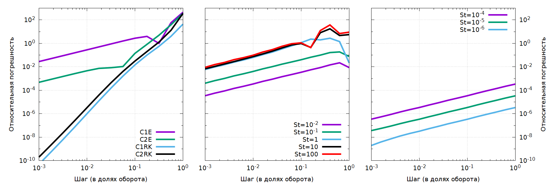
Figure 12: The left panel shows the relative error in the solution of the system without friction after 40 orbital periods [the integrals (29), (30)], obtained using the first- and fourth-order methods in the time step, the central and right panels the errors in $v_{r}$ in the solution of the system with drag using the first-order semi-implicit method for various Stokes numbers. The integration time was two orbital periods for the central panel and 40 orbital periods for the right panel.

At the initial time, we placed the particle at the radius $r_{0}=10$ au and specified its radial velocity to be close to zero and its azimuthal velocity to be the Keplerian value. We computed the particle’s trajectory over a time $t=40\times 2\pi\Omega^{-1}(r_{0})$ (40 orbits around the central body) using an explicit Euler method (into which the semi-implicit, first-order scheme with zero drag is degenerate) and the explicit Runge–Kutta method. At the final time, we calculated the values of $C_{1}$ and $C_{2}$ and compared them to the initial values of these integrals. The dependence of the relative errors in $C_{1}$ and $C_{2}$ on the time step $\tau$ re presented in the left panel of Fig. 12. Both schemes give the stated order of approximation in the solution, with the accuracy of the computation of the angular momentum in the first-order scheme being almost a factor of 100 worse than the accuracy of the computation of the energy. Computing $C_{1}$ with an accuracy of up to 1% using the first-order scheme requires more than 1000 steps in one orbit of the central body, whereas 10 steps per orbit is sufficient for the Runge–Kutta method.

We also studied how many steps per orbit are required by the first-order scheme in order to obtain an accuracy of 1% when drag force is added to the system (27). We solved the system (27), where the components of the drag force have the form $\left(\displaystyle\frac{(v_{r}-u_{r})\Omega(r)}{\rm{St}},\displaystyle\frac{(v_{\varphi}-u_{\varphi})\Omega(r)}{\rm{St}}\right)$ with the constant value of $\rm{St}$. For $\rm{St}=10^{-6},\quad 10^{-5},\quad 10^{-4}$ we carried out the integration over a time $t=40\times 2\pi\Omega^{-1}(r_{0})$, and for $\rm{St}=10^{-2},\quad 10^{-1},\quad 1,\quad 10,\quad 100$ over the shorter time $t=2\times 2\pi\Omega^{-1}(r_{0})$. We used the solution of this same problem obtained using the fourth-order method with a time resolution of $10^{7}$ steps per orbit $t=2\pi\Omega^{-1}(r_{0})$, as a reference. The relative errors in $v_{r}$, computed in the semi-implicit, first-order scheme are presented in the central and right panels of Fig. 12. For all values of $\rm{St}$ the semi-implicit scheme demonstrates first-order in its approximation, but the actual accuracy attained in the solution depends on $\rm{St}$. In the computations presented in the right panel, $\rm{St}\ll 1$, and the dynamics of the particle are determined by the gas drag, not by the balance between centrifugal and gravitational forces. In these computations, the lower the value of $\rm{St}$, the higher the accuracy of the numerical solution. In the computations with $\rm{St}\geq 1$, presented in the central panel, the dynamics of the particle are determined by the balance between the centrifugal and gravitational forces, and the actual accuracy in $v_{r}$ does not depend on $\rm{St}$ ,and is close to the accuracy with which $C_{1}$ is calculated in the computations without friction using the same time steps.

On the whole, the data presented in Fig. 12 and Table 1 show the expediency of using the first-order scheme for simulations of the dynamics of particles in a disk at orbital radii greater than 1 au.

4 CONCLUSION

The sizes of dust grains in circumstellar and protoplanetary disks vary from submicron to several centimeters, and planetesimals have sizes of hundreds of kilometers. Therefore, the exchange of momentum between solid bodies and gas in disks occurs in a variety of regimes, determined by the sizes and velocities of the solid bodies: Epstein, Stokes, and Newton. We have compared different drag coefficients encompassing these regimes. We have shown that the standard astrophysical drag coefficient (8) is a discontinuous function for Mach numbers corresponding to the motion of the grains relative to the gas $\rm{Ma}>1/9$, but is continuous when $\rm{Ma}<1/9$. Application of the standard astrophysical coefficient in simulations of circumstellar disks with $\rm{Ma}<1/9$ is justified by the speed of the computations. When $\rm{Ma}>1/9$, it is recommended to use the Henderson drag coefficient (10)–(13), which is valid and continuous when $\rm{Ma}<6$, $\rm{Re}<3\times 10^{5}$. Each computation of the Henderson coefficient requires of about 100 arithmetic operations.

In addition, the need to compute the dynamics of bodies of different sizes in the same way imposes high demands on numerical methods used for this purpose. We have shown that our semi-implicit, first-order approximation scheme, in which the interphase interactions are linearized and the relative velocity is calculated implicitly, while the stopping time and other forces, such as the pressure gradient and gravitation are calculated explicitly, preserve the asymptotic behavior of the solutions of problems with intense interphase interactions. This means that the scheme is suitable for computing the dynamics of both small bodies that are strongly coupled to the gas and larger bodies for which the drag force depends non-linearly on the relative velocity between the gas and bodies, including the influence of the dispersed phase on the gas dynamics.

Appendix A APPROACH TO DESCRIBING THE DYNAMICS OF DUST IN A CIRCUMSTELLAR DISK

The suitability of a hydrodynamical approach to describing a medium is usually determined using two conditions:

• The mean free path of the particles making up the medium should be much shorter than the length scale of the system. We will take the disk scale height $H$ as a length scale of the system.

Further, some element of the medium is distinguished whose size is much less than the length scale of the medium, but much larger than the mean free path of the particles. In our case, this is the size of a computational grid cell, $\delta R$.

• The number of particles in a given volume of the medium $\delta R$ should be sufficiently large.

The first condition is required so that the loss/gain of particles by an element of the medium as a result of chaotic motions of the particles does not appreciably influence the mean characteristics of the element. The second condition is required for computations using the particle distribution function in the six-dimensional space (coordinates and velocities) of the mean characteristics, such as the mean density in a cell, the mean velocity, and the mean energy.

There is no doubt that these conditions are satisfied by the gas in a circumstellar disk. However, we must investigate this question for the dust component. We estimated the mean free path of a solid particle assuming that the dust subdisk consists of monodisperse, spherical particles. In this case,

$$\lambda_{\rm d}=\displaystyle\frac{1}{\sqrt{2}\pi a^{2}n_{\rm d}}=\displaystyle\frac{4a\rho_{\rm s}}{2\sqrt{2}\rho_{\rm d}},$$ (31)

since, by virtue of their monodisperse nature,

$$n_{\rm d}(a)=\displaystyle\frac{3\rho_{\rm d}}{4\pi\rho_{\rm s}a^{3}}.$$ (32)

We assumed that the volume density of the dust in the equatorial plane of the disk was given by

$$\rho_{\rm d}=\frac{\Sigma_{\rm d}}{H\sqrt{\pi}},$$ (33)

where the height of the disk is

$$H=\sqrt{\frac{2k_{\rm B}T}{\mu_{\rm H}}\frac{r^{3}}{GM}}$$ (34)

Let the surface density of the dust and the temperature be power-law functions of the radius, $\Sigma_{\rm d}(r)=\Sigma_{0}(r/1\,{\textrm{AU}})^{p}$, $T=T_{0}(r/1\,{\textrm{AU}})^{q}$. Adopting the characteristic values for a circumstellar disk $\Sigma_{0}=1$ g cm^-2, $T_{0}$=300 K, $\mu_{\rm H}=2.3$, $M=1M_{\odot}$, $p=-1,q=-0.5$, we obtain

$$\rho_{\rm d}=7.6\cdot 10^{-13}(r/1\,{\textrm{AU}})^{-2.25}\quad{\textrm{g\leavevmode\nobreak\ cm}}^{-3}.$$ (35)

It follows from (31) and (35)that grains smaller than 1 cm in the outer parts of a disk have mean free paths much shorter than $\delta R$. It is clear that the dust subdisk can be modeled as a continuous medium in this case. On the other hand, these estimates indicate that $\lambda_{\rm d}$ is close to $H$ in inner regions of the disk. In this case, instead of the mean velocity over the volume, we must consider the velocity of the solid phase as a vector plus a dispersion. A possible development of the model could be the use of the Vlasov–Boltzmann equation [35] or moments of the Boltzmann equation [44]. The solution of the Vlasov–Boltzmann equation in Lagrange coordinates implies the use of discrete particles when modeling the dynamics of the solid phase [5, 50, 48]. Solution for the moment Boltzmann equation can be found in an Euler approach using grid methods [45].

The moment Boltzmann equation take into account the possible anisotropic behaviour of the velocity dispersion of the medium, but computing the components of the velocity dispersion requires the introduction of additional equations. When solving the Vlasov–Boltzmann equation using a particle method, the velocity dispersion varies in a self-consistent way [9], but the difficulty is correctly computing the collision integral. In gas dynamics, this integral is zero for frequent elastic collisions. This may not be the case for the grains.

We have concluded that dust in the main part of the disk can be represented as a continuous medium, while there may be regimes in the central region of the disk in which solid particles have a velocity dispersion, based on estimates of the mean free paths of particles, neglecting their interactions with the gas. However, the same conclusion is supported by estimates of the spatial scale on which exchanges of momentum between the gas and dust occur:

$$\lambda_{\rm stop}=\|u-v\|t_{\rm stop},$$ (36)

where $t_{\rm stop}={\rm St}/\Omega_{\rm K}$. According to [8] Eq.(8), the azimuthal velocity of a particle can be estimated as

$$u=v_{\rm K}\left(1-\frac{1}{1+{\rm St}^{2}}\eta\right).$$ (37)

Here, $\eta$ characterizes the degree of deviation of the velocity of the gas from the Keplerian value, and, for typical disk parameters, $\eta\sim 0.01$. We then find that

$$\lambda_{\rm stop}=r{\rm St}\left(1-\frac{1}{1+{\rm St}^{2}}\eta\right)\sim r{\rm St}.$$ (38)

It is clear that, when $St<0.01$, the velocities of grains within a single cell will differ little, while they will differ appreciably when $St\sim 1$. The simulation results [43] indicate that dust that has grown is located in the inner part of the disk.

Appendix B MODEL OF A STATIONARY GASEOUS DISK

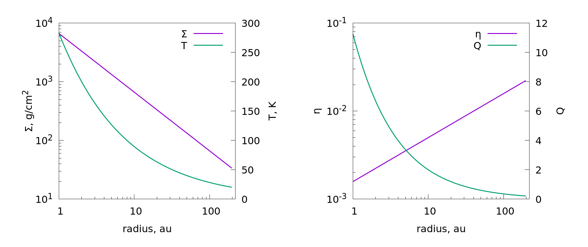
Figure 13: (Left panel) Radial distributions of the surface density and temperature in a circumstellar disk for Toy Models 1 and 2. (Right panel) Radial distribution of $\eta$ and Toomre parameter for Toy Models 1 and 2.

We calculated the radial distributions of parameters of an axially symmetric, gaseous disk with inner boundary $R_{\rm min}$ and outer boundary $R_{\rm max}$ with mass $M_{\rm disk}$ around a star with mass $M$ using the model of [33], which is based on the following assumptions:

• the surface density of the matter in the disk displays a power-law dependence on the radius with power-law index $\xi$:

  $$\Sigma(r)=\Sigma_{0}\left(\frac{r}{R_{0}}\right)^{-\xi},$$ (39)

  where $\Sigma_{0}R_{0}^{\xi}$ is given by

  $$\int_{0}^{2\pi}\int_{R_{\rm min}}^{R_{\rm max}}\Sigma(r)r\,dr\,d\varphi=M_{\rm{disk}},$$ (40)

• the density and temperature of the gas in the disk are such that the Toomre parameter varies as

  $$Q(r)=\frac{c_{s}(r)\Omega(r)}{\pi G\Sigma(r)}=2\left(\frac{R_{\rm{max}}}{r}\right)^{0.75},$$ (41)

• the gaseous disk is in equilibrium, so that

  $$u_{r}=0,\quad u_{\varphi}(r)=\sqrt[]{\displaystyle\frac{GM}{r}+\frac{r}{\rho_{\rm g}(r)}\frac{dp(r)}{dr}},$$ (42)

• the height $H$ and radius $r$ of the disk are related as

  $$\frac{c_{\rm s}(r)}{V_{\rm K}(r)}=\frac{H(r)}{r},$$ (43)

• the gas density at each radius does not vary in the vertical direction, so

  $$\rho_{\rm g}(r)=\displaystyle\frac{\Sigma(r)}{H(r)}.$$ (44)

We assumed $\xi=1$ and used the above assumptions to find the distributions $c_{\rm s}(r)$, $\rho_{\rm g}(r)$, $u_{\varphi}(r)$ in the disk, which are required for the solution of (27).

It follows from (40) that

$$\Sigma_{0}=\frac{M_{\rm{disk}}(2-\xi)}{2\pi R_{0}^{\xi}(R_{\rm{max}}^{2-\xi}-R_{\rm{min}}^{2-\xi})}.$$ (45)

It follows from (41) that

$$c_{s}(r)=\frac{Q(r)\pi G\Sigma(r)}{\Omega(r)}=\frac{\pi rQ(r)G\Sigma(r)}{V_{\rm K}(r)},$$ (46)

and therefore

$$\frac{c_{s}(r)}{V_{\rm K}(r)}=\frac{\pi Q(r)G\Sigma(r)r}{V_{\rm K}^{2}}=\frac{\pi Q(r)\Sigma(r)r^{2}}{M}.$$ (47)

We then obtain from (47) and (43)

$$H(r)=\displaystyle\frac{\pi Q(r)\Sigma(r)r^{3}}{M},$$ (48)

whence

$$\rho_{\rm g}(r)=\displaystyle\frac{\Sigma(r)}{H(r)}=\frac{M}{\pi Q(r)r^{3}}.$$ (49)

Note that, by virtue of (41)

$$\rho_{\rm g}(r)=\rho_{\rm g0}\displaystyle\left(\frac{r}{R_{0}}\right)^{-2.25}.$$ (50)

We took $u_{\varphi}$ to be related to $V_{\rm K}$ as

$$u_{\varphi}^{2}=V_{\rm K}^{2}+\left(\frac{d\ln\rho_{\rm g}}{d\ln r}\right)c_{s}^{2}=V_{\rm K}^{2}(1-\eta),$$ (51)

where

$$\eta=\frac{c_{s}^{2}}{V_{\rm K}^{2}}\left|\frac{d\ln\rho_{\rm g}}{d\ln r}\right|=2.25\frac{c_{s}^{2}}{V_{\rm K}^{2}}=\frac{2.25\pi^{2}Q^{2}(r)\Sigma^{2}(r)r^{4}}{M^{2}},$$ (52)

so that

$$u_{\varphi}=V_{\rm K}\,\sqrt[]{1-\frac{2.25\pi^{2}Q^{2}(r)\Sigma^{2}(r)r^{4}}{M^{2}}}=V_{\rm K}\,\sqrt[]{1-\frac{2.25\Sigma^{2}(r)}{\rho^{2}_{\rm g}(r)r^{2}}}$$ (53)

The distribution of the surface density and temperature for the disk in Toy Models 1 and 2 is shown in Fig. 13.

Appendix C ACKNOWLEDGMENTS

We thank V.N. Snytnikov and M.I. Osadchii for productive discussions of our results.

Appendix D FUNDING

This work was founded by the Russian Science Foundation (grant 17-12-01168).

References

- [1] V. V. Akimkin, M. S. Kirsanova, Y. N. Pavlyuchenkov, and D. S. Wiebe. Dust dynamics and evolution in expanding H II regions. I. Radiative drift of neutral and charged grains. MNRAS, 449:440–450, May 2015.
- [2] V. V. Akimkin, M. S. Kirsanova, Y. N. Pavlyuchenkov, and D. S. Wiebe. Dust dynamics and evolution in H ii regions - II. Effects of dynamical coupling between dust and gas. MNRAS, 469:630–638, July 2017.
- [3] G. Albi, G. Dimarco, and L. Pareschi. Implicit-Explicit multistep methods for hyperbolic systems with multiscale relaxation. arXiv e-prints, page arXiv:1904.03865, Apr 2019.
- [4] G.h Bagheri and C. Bonadonna. On the drag of freely falling non-spherical particles. Powder Technology, 301:526–544, 06 2016.
- [5] X.-N. Bai and J. M. Stone. Particle-gas Dynamics with Athena: Method and Convergence. ApJSS, 190:297–310, October 2010.
- [6] L. Barrière-Fouchet, J.-F. Gonzalez, J. R. Murray, R. J. Humble, and S. T. Maddison. Dust distribution in protoplanetary disks. Vertical settling and radial migration. AAp, 443:185–194, November 2005.
- [7] P. Benítez-Llambay, L. Krapp, and M. E. Pessah. Asymptotically Stable Numerical Method for Multispecies Momentum Transfer: Gas and Multifluid Dust Test Suite and Implementation in FARGO3D. ApJSS, 241:25, April 2019.
- [8] T. Birnstiel, M. Fang, and A. Johansen. Dust Evolution and the Formation of Planetesimals. Space Science Reviews, 205:41–75, December 2016.
- [9] R. A. Booth and C. J. Clarke. Collision velocity of dust grains in self-gravitating protoplanetary discs. MNRAS, 458:2676–2693, May 2016.
- [10] S.-H. Cha and S. Nayakshin. A numerical simulation of a ’Super-Earth’ core delivery from 100 to 8 au. MNRAS, 415:3319–3334, August 2011.
- [11] G.-Q. Chen, C. D. Livermore, and T.-P. Liu. Hyperbolic conservation laws with stiff relaxation terms and entropy. Communications in Pure and Applied Mathematics, 47:787–830, june 1994.
- [12] P. Colella and P. R. Woodward. The Piecewise Parabolic Method (PPM) for Gas-Dynamical Simulations. Journal of Computational Physics, 54:174–201, September 1984.
- [13] N. Cuello, J.-F. Gonzalez, and F. C. Pignatale. Effects of photophoresis on the dust distribution in a 3D protoplanetary disc. MNRAS, 458:2140–2149, May 2016.
- [14] T. V. Demidova and V. P. Grinin. SPH simulations of structures in protoplanetary disks. Astronomy Letters, 43:106–119, February 2017.
- [15] P. S. Epstein. On the Resistance Experienced by Spheres in their Motion through Gases. Physical Review, 23:710–733, June 1924.
- [16] T. J. Haworth, J. D. Ilee, D. H. Forgan, S. Facchini, D. J. Price, D. M. Boneberg, R. A. Booth, C. J. Clarke, J.-F. Gonzalez, M. A. Hutchison, I. Kamp, G. Laibe, W. Lyra, F. Meru, S. Mohanty, O. Panić, K. Rice, T. Suzuki, R. Teague, C. Walsh, P. Woitke, and Community authors. Grand Challenges in Protoplanetary Disc Modelling. PASA, 33:e053, October 2016.
- [17] C. B. Henderson. Drag coefficient of spheres in continuum and rarefied flows. AIAA Journal, 14:707–707, 1976.
- [18] M. Hutchison, D. J. Price, and G. Laibe. MULTIGRAIN: a smoothed particle hydrodynamic algorithm for multiple small dust grains and gas. MNRAS, 476:2186–2198, May 2018.
- [19] S. Ishiki, T. Okamoto, and A. K. Inoue. The effect of radiation pressure on dust distribution inside HII regions. MNRAS, 474(2):1935–1943, 2018.
- [20] S. Jin and C. D. Livermore. Numerical Schemes for Hyperbolic Conservation Laws with Stiff Relaxation Terms. Journal of Computational Physics, 126:449–467, 1996.
- [21] A. Johansen and H. Klahr. Dust Diffusion in Protoplanetary Disks by Magnetorotational Turbulence. ApJ, 634:1353–1371, December 2005.
- [22] G. Laibe and D. J. Price. Dusty gas with smoothed particle hydrodynamics - I. Algorithm and test suite. MNRAS, 420:2345–2364, March 2012.
- [23] G. Laibe and D. J. Price. Dusty gas with smoothed particle hydrodynamics - II. Implicit timestepping and astrophysical drag regimes. MNRAS, 420:2365–2376, March 2012.
- [24] G. Laibe and D. J. Price. Dust and gas mixtures with multiple grain species - a one-fluid approach. MNRAS, 444:1940–1956, October 2014.
- [25] G. Laibe and D. J. Price. Dusty gas with one fluid. MNRAS, 440:2136–2146, May 2014.
- [26] L.D. Landau and E.M. Lifshitz. Fluid Mechanics. Vol. 6 (2nd ed.). Butterworth-Heinemann, 1987.
- [27] P. Lorén-Aguilar and M. R. Bate. Two-fluid dust and gas mixtures in smoothed particle hydrodynamics: a semi-implicit approach. MNRAS, 443:927–945, September 2014.
- [28] P. Lorén-Aguilar and M. R. Bate. Two-fluid dust and gas mixtures in smoothed particle hydrodynamics II: an improved semi-implicit approach. MNRAS, 454:4114–4119, December 2015.
- [29] J. J. Monaghan and A. Kocharyan. SPH simulation of multi-phase flow. Computer Physics Communications, 87:225–235, May 1995.
- [30] Y. Nakagawa, M. Sekiya, and C. Hayashi. Settling and growth of dust particles in a laminar phase of a low-mass solar nebula. Icarus, 67:375–390, September 1986.
- [31] R. Pember. Numerical methods for hyperbolic conservation laws with stiff relaxation i. spurious solutions. SIAM Journal on Applied Mathematics, 53:1293–1330, February 1993.
- [32] R. F. Probstein and F. Fassio. Dusty Hipersonic Flows. AIAA Journal, 8:772–779, 1970.
- [33] W. K. M. Rice, G. Lodato, J. E. Pringle, P. J. Armitage, and I. A. Bonnell. Accelerated planetesimal growth in self-gravitating protoplanetary discs. MNRAS, 355:543–552, December 2004.
- [34] D.V. Sadin and S.A. Odoev. Comparison of difference scheme with customizable dissipative properties and weno scheme in the case of one-dimensional gas and gas-particle dynamics problems. Scientific and Technical Journal of Information Technologies, Mechanics and Optics, pages 719–724, 07 2017.
- [35] V. N. Snytnikov and O. P. Stoyanovskaya. Clump formation due to the gravitational instability of a multiphase medium in a massive protoplanetary disc. MNRAS, 428:2–12, January 2013.
- [36] J. M. Stone and M. L. Norman. ZEUS-2D: A radiation magnetohydrodynamics code for astrophysical flows in two space dimensions. I - The hydrodynamic algorithms and tests. ApJSS, 80:753–790, June 1992.
- [37] O. P. Stoyanovskaya, V. V. Akimkin, E. I. Vorobyov, T. A. Glushko, Y. N. Pavlyuchenkov, V. N. Snytnikov, and N. V. Snytnikov. Development and application of fast methods for computing momentum transfer between gas and dust in supercomputer simulation of planet formation. In Journal of Physics Conference Series, volume 1103 of Journal of Physics Conference Series, page 012008, October 2018.
- [38] O. P. Stoyanovskaya, T. A. Glushko, N. V. Snytnikov, and V. N. Snytnikov. Two-fluid dusty gas in smoothed particle hydrodynamics: Fast and implicit algorithm for stiff linear drag. Astronomy and Computing, 25:25–37, October 2018.
- [39] O. P. Stoyanovskaya, N. V. Snytnikov, and V. N. Snytnikov. Modeling circumstellar disc fragmentation and episodic protostellar accretion with smoothed particle hydrodynamics in cell. Astronomy and Computing, 21:1–14, October 2017.
- [40] O. P. Stoyanovskaya, V. N. Snytnikov, and E. I. Vorobyov. Analysis of methods for computing the trajectories of dust particles in a gas-dust circumstellar disk. Astron.Rep., 94:1033–1049, December 2017.
- [41] D V. Sadin. Tvd scheme for stiff problems of wave dynamics of heterogeneous media of nonhyperbolic nonconservative type. Computational Mathematics and Mathematical Physics, 56:2068–2078, 12 2016.
- [42] E. I. Vorobyov. Embedded Protostellar Disks Around (Sub-)Solar Protostars. I. Disk Structure and Evolution. ApJ, 723:1294–1307, November 2010.
- [43] E. I. Vorobyov, V. Akimkin, O. Stoyanovskaya, Y. Pavlyuchenkov, and H. B. Liu. Early evolution of viscous and self-gravitating circumstellar disks with a dust component. Astronomy and Astrophysics, 614:A98, June 2018.
- [44] E. I. Vorobyov and C. Theis. Boltzmann moment equation approach for the numerical study of anisotropic stellar discs. MNRAS, 373:197–208, November 2006.
- [45] E. I. Vorobyov and C. Theis. Shape and orientation of stellar velocity ellipsoids in spiral galaxies. MNRAS, 383:817–830, January 2008.
- [46] S. J. Weidenschilling. Aerodynamics of solid bodies in the solar nebula. MNRAS, 180:57–70, July 1977.
- [47] F. L. Whipple. On certain aerodynamic processes for asteroids and comets. In A. Elvius, editor, From Plasma to Planet, page 211, 1972.
- [48] C.-C. Yang and A. Johansen. Integration of Particle-gas Systems with Stiff Mutual Drag Interaction. ApJS, 224:39, June 2016.
- [49] Z. Zhu, R. P. Nelson, R. Dong, C. Espaillat, and L. Hartmann. Dust Filtration by Planet-induced Gap Edges: Implications for Transitional Disks. ApJ, 755:6, August 2012.
- [50] Z. Zhu and J. M. Stone. Dust Trapping by Vortices in Transitional Disks: Evidence for Non-ideal Magnetohydrodynamic Effects in Protoplanetary Disks. ApJ, 795:53, November 2014.