On the Optimal Duration of Spectrum Leases in Exclusive License Markets with Stochastic Demand

Abstract

This paper addresses the following question which is of interest in designing efficient exclusive-use spectrum licenses sold through spectrum auctions. Given a system model in which customer demand, revenue, and bids of wireless operators are characterized by stochastic processes and an operator is interested in joining the market only if its expected revenue is above a threshold and the lease duration is below a threshold, what is the optimal lease duration which maximizes the net customer demand served by the wireless operators? Increasing or decreasing lease duration has many competing effects; while shorter lease duration may increase the efficiency of spectrum allocation, longer lease duration may increase market competition by incentivizing more operators to enter the market. We formulate this problem as a two-stage Stackelberg game consisting of the regulator and the wireless operators and design efficient algorithms to find the Stackelberg equilibrium of the entire game. These algorithms can also be used to find the Stackelberg equilibrium under some generalizations of our model. Using these algorithms, we obtain important numerical results and insights that characterize how the optimal lease duration varies with respect to market parameters in order to maximize the spectrum utilization. A few of our numerical results are non-intuitive as they suggest that increasing market competition may not necessarily improve spectrum utilization. To the best of our knowledge, this paper presents the first mathematical approach to optimize the lease duration of spectrum licenses.

I Introduction

With the rapid growth of wireless services and devices, wireless data traffic is increasing. Cisco’s forecast [2] shows a 6-fold increase in global data traffic from 2017 to 2022. There is only a finite amount of wireless spectrum that can be used to support the growing wireless data traffic. There are various reports [3, 4] that show that many licensed spectrum channels are underutilized, leading to inefficient use of the spectrum. It is widely accepted that the legacy policy of static spectrum allocations is a major cause of inefficient spectrum utilization [5]. Long-term spectrum leases can also lead to spectrum hoarding [6]. Long-term spectrum leases are likely to have higher license fees. Higher license fees lead to a lower number of wireless operators in the market and can also lead to collusion among wireless operators [7]. This can reduce market competition and hence may lead to inefficient spectrum utilization. For the recently proposed Citizens Broadband Radio Service band [8], the lease duration of Priority Access Licenses (PAL) is an important topic of debate. Since potential wireless operators prefer different lease duration of PALs, it has changed multiple times over the last few years of debate; $1$ year in $2015$ [8], $3$ years in $2016$ [9], $10$ years in $2017$ [10]. In spite of the importance of lease duration, there is no formal study to optimize lease duration (except for our previous work [1]).

In this paper, we present a mathematical model to capture the effect of lease duration on spectrum utilization when channels are allocated for exclusive use. Our model can be summarized as follows. First, the customer demand, the revenue of an operator and its bids are modeled as statistically correlated stochastic processes. Second, spectrum utilization is equal to the net customer demand served by the operators over a long time horizon. Third, the revenue of an operator and its valuation of channel is solely dependent on the amount of customer demand it can serve using the channel; the more the customer demand served by the operator, the higher its revenue and valuation of the channel. Fourth, an operator will join the market only if the lease duration is below a threshold so that it can afford the licensing fees and if the lease duration is such that its expected revenue is above a threshold so that it can generate return sufficient return on its investments.

Based on our system model, we formulate an optimization problem whose objective is to maximize spectrum utilization. The optimization problem manifests itself as a two-stage Stackelberg game consisting of the regulator and the wireless operators. The optimization problem, in essence, has only one scalar decision variable, the lease duration. Shorter lease duration increases the frequency of spectrum auctions. Therefore, there is frequent re-allocation of channels to those operators who values it the most. This leads to more efficient allocation of spectrum and hence improves spectrum utilization. On the other hand, longer lease duration, in general, ensures that the operators get their desired return on investment. This incentivizes more operators to join the market and hence lead to more competition which in turn improves spectrum utilization. However, if the lease duration is too long, some of the operators may not join the market because they cannot afford license fees [10]. These opposing factors suggest that the optimization problem should have a non-trivial solution.

There have been several active areas of research related to spectrum licenses, such as pricing [11], auction design [12], flexible licensing [13], enforcement [14], etc. But, to the best of our knowledge, a mathematical treatment of the impact of lease duration of spectrum licenses has been only considered in [15]. In [15], the authors took a data-driven approach and concluded that lease duration has no significant impact on spectrum market competition. But there are several works like [5, 6, 7] that suggest otherwise and also data-driven approaches cannot be generalized, especially for extrapolation. Furthermore, higher market competition may not necessarily imply higher spectrum utilization as we show in section IV. Other than [15], we found no paper that mathematical studies the impact of lease duration even in other synergistic areas such as electricity markets and cloud computing.

However, there are a few works in the spectrum sharing literature that consider the effect of certain “duration aspects” on the overall performance of the system. The work in [16] considers a market of only two service providers with a common customer base. Time is divided into intervals. At the beginning of every interval, an auction is conducted which redistributes the available bandwidth based on the bids of individual service providers. The ratio of the customer demand reaching each service provider is governed by evolutionary game theory. The authors use simulations to conclude that shorter allocation interval corresponds to better spectrum utilization. In [17], the authors model various factors that a secondary service provider considers when buying spectrum resources from primary service providers. The authors design a utility function for the secondary service provider that suggest that longer contract duration is better. In [18], the primary user leases its bandwidth to secondary users for a fraction of time in exchange for cooperation (relaying). If the fraction of time is too small, it will not compensate for the overall cost of transmission (including relaying), and hence the secondary users may not agree to cooperate. For opportunistic spectrum use, optimal spectrum sensing time is an area which received wide attention from the spectrum community [19]. There are few works in economic journals like [20] that consider the problem of optimizing contract duration for welfare analysis. The fundamental idea governing these works is a tradeoff between opportunity cost and transaction cost. The definitions of transaction cost and opportunity cost change with the market setting, like housing property market [21], priority service market [22], etc.

In Section II-A, we present a system model to study the effect of lease duration on spectrum utilization. Our model captures important properties of the effect of lease duration and market competition on spectrum utilization and an operator’s expected revenue. We also discuss how some of these properties are affected by bidding accuracy, the statistical correlation between an operator’s bid and its revenue. These properties are discussed in Section II-C. Up to our knowledge, this is the first system model that enables the mathematical analysis of optimal lease duration. This constitutes the first contribution of the paper. The work done in this paper extends to other system models as long as it satisfies the properties discussed in Section II-C. Few of these generalizations are hypothesized in Section II-C as well.

In Section III-A, we capture the interaction between a regulator and the operators as a two-stage Stackelberg game with incomplete information. In the first stage, the regulator sets the lease duration to optimize spectrum utilization. In the second stage (subgame), the operators decide whether to enter the market or not based on the lease duration set by the regulator in the first stage. Our model admits an unique subgame Nash equilibrium (NE) and hence finding the Stackelberg Equilibrium of the two-stage Stackelberg game reduces to solving the optimization problem of the first stage which has only one scalar decision variable, the lease duration. Yet, the optimization problem is not trivial because it is reminiscent of combinatorial optimization. To elaborate, the debate over lease duration of PALs shows that it may not be possible to choose a lease duration which interests all the operators. In fact, a lease duration which interests all the operators, even if it exists, may not lead to the optimal spectrum utilization. Hence, in certain sense, we want to find the optimal set of interested operators which is a combinatorial optimization problem. The formulation of the Stackelberg game is the second contribution of the paper.

In Section III, we design algorithms to solve the optimization problem of the first stage for two scenarios: (i) homogeneous market with complete information, (ii) heterogeneous market with incomplete information. Since the optimization problem has a combinatorial nature, the number of candidate sets of interested operators may be exponential in the number of operators in the market. The design of an efficient optimization algorithm relies on the result that, with lease duration as the decision variable, the number of candidate sets of interested operators is polynomial in the number of operators in the market. Designing an efficient optimization algorithm for the first stage game is the third contribution of the paper. The final contribution is the numerical results presented in Section IV. We use our optimization algorithm to numerically study the variation of optimal characteristics, i.e., optimal lease duration and optimal value of the objective function, as a function of market parameters. We also study how bidding accuracy and incomplete information decreases spectrum utilization. Few of our numerical results are non-intuitive as they suggest that increasing market competition may not necessarily improve spectrum utilization.

II Problem Formulation

We present our system model in Section II-A and also introduce the revenue function and the objective function, which capture the revenue of an operator and spectrum utilization, respectively. The expressions of the revenue and the objective function are derived in Section II-B. The properties of the objective and the revenue function are discussed in Section II-C which reveal their practical relevance. We also discuss few generalizations of our system model in Section II-C. Table I lists frequently used notations while other notations are standard.

Table I: A table of frequently used notations.

Notation	Description
$\mathbb{Z}^{+}$	Set of positive integers.
$\left\lceil x\right\rceil$	Ceiling Function.
$T$	Lease duration.
$N$	Number of operators.
$M$	Number of channels.
$x_{k}\left(t\right)$	Revenue of the $k^{th}$ operator in $t^{th}$ time slot.
$Y_{k}\left(c,T\right)$	Net revenue of the $k^{th}$ operator in $c^{th}$ epoch if lease duration is $T$.
$\widehat{Y}_{k}\left(c,T\right)$	Bid of the $k^{th}$ operator in $c^{th}$ epoch if lease duration is $T$.
$\mu_{k}$ , $\widehat{\mu}_{k}$	True and estimated mean respectively of the revenue process of the $k^{th}$ operator.
$\sigma_{k}$ , $\widehat{\sigma}_{k}$	True and estimated standard deviation respectively of the revenue process of the $k^{th}$ operator.
$a_{k}$ , $\widehat{a}_{k}$	True and estimated autocorrelation coefficient respectively of the revenue process of the $k^{th}$ operator.
$\rho_{k}$ , $\widehat{\rho}_{k}$	True and estimated bid correlation coefficient respectively of the $k^{th}$ operator.
$\lambda_{k}$ , $\widehat{\lambda}_{k}$	True and estimated minimum expected revenue (MER) requirement respectively of the $k^{th}$ operator.
$\Lambda_{k}$ , $\widehat{\Lambda}_{k}$	True and estimated maximum lease duration respectively above which the $k^{th}$ operator cannot afford a channel.
$\xi_{k}$ , $\widehat{\xi}_{k}$	Tuples representing the true and estimated parameters of the $k^{th}$ operator resp. We have, $\xi_{k}=\left(\mu_{k},\sigma_{k},a_{k},\rho_{k},\lambda_{k},\Lambda_{k}\right)$ and $\widehat{\xi}_{k}=\left(\widehat{\mu}_{k},\widehat{\sigma}_{k},\widehat{a}_{k},\widehat{\rho}_{k},\widehat{\lambda}_{k},\widehat{\Lambda}_{k}\right)$.
$\mathcal{S}$	Set of interested operators.
$s$	Number of interested operators. We have $s=\left|\mathcal{S}\right|$.
$\widetilde{S}$	Set of interested operators according to the regulator.
$\mathcal{S}_{k}^{L}$	Largest set of interested operators who may join the market according to the $k^{th}$ operator.
$\widetilde{S}^{L}$	Largest set of interested operators according to the regulator.
$\mathcal{R}_{k}\left(\mathcal{S},T\right)$	Revenue function of the $k^{th}$ operator.
$\widehat{\mathcal{R}}_{k}\left(\mathcal{S},T\right)$	Revenue function of the $k^{th}$ operator as perceived by itself.
$\widetilde{\mathcal{R}}_{k}\left(\mathcal{S},T\right)$	Revenue function of the $k^{th}$ operator as perceived by the regulator.
$U\left(\mathcal{S},T\right)$	Objective function as a function of set of interested operators $\mathcal{S}$ and lease duration $T$.
$\widetilde{U}\left(\mathcal{S},T\right)$	Objective function as perceived by the regulator as a function of set of interested operators $\mathcal{S}$ and lease duration $T$.
$U\left(T\right)$	Objective function as a function of lease duration $T$.
$\widetilde{U}\left(T\right)$	Objective function as perceived by the regulator as a function of lease duration $T$.
$\mathcal{R}\left(s,T\right)$	Revenue function of an operator for a market that is homogeneous in $\mu_{k}$, $\sigma_{k}$, $a_{k}$ and $\rho_{k}$.
$U\left(s,T\right)$	Objective function as a function of number of interested operators $s$ and lease duration $T$. It only applies for a market that is homogeneous in $\mu_{k}$, $\sigma_{k}$, $a_{k}$ and $\rho_{k}$.

II-A System Model

We consider a time slotted model where $t\in\mathbb{Z}^{+}$ is a time slot. Let $T\in\mathbb{Z}^{+}$ denote the lease duration. The word epoch denotes a lease duration. Hence, the time slots corresponding to the $c^{th}$ epoch are $t\in\left[\left(c-1\right)T+1\,,\,cT\right]$ where $c\in\mathbb{Z}^{+}$. There are $N$ operators indexed $k=1,2,\ldots,N$. Let $\mathcal{S}\subseteq\left\{1,2,\ldots,N\right\}$ be the set of operators who are interested in entering the market. In our model, the number of interested operators, $s=\left|\mathcal{S}\right|$, is the measure of market competition [15]. There are $M$ channels indexed $m=1,2,\ldots,M$ which are to be allocated to the operators in set $\mathcal{S}$, at the beginning of every epoch, for exclusive use. Similar to prior works like [23, 24], these channels are assumed to be identical. Our model assumes spectrum cap of one, i.e. an operator is allocated at most one channel in every epoch.

Let $x_{k}\left(t\right)$ denonte the revenue of the $k^{th}$ operator at time slot $t$ if it is allocated a channel. The revenue of an operator is $0$ if it is not allocated a channel. We model the revenue $x_{k}\left(t\right)$ as a first order Gaussian Autoregressive (AR) process. Modeling time-series with AR models is a common practice in academic literature [25, 26]. Federal Communication Commission report [9] expresses the need for “periodic, market-based reassignment of channels in response to changes in local conditions and operator needs.” A first order AR process is a simple stochastic process capturing autocorrelation among time series data. We can model fast (slow) “changes in local conditions and operator needs” by setting a lower (higher) autocorrelation among $x_{k}\left(t\right)$. Mathematically,

$$x_{k}\left(t+1\right)=a_{k}x_{k}\left(t\right)+\varepsilon_{k}\left(t\right)\>;\>\forall t\geq 1$$ (1)

where $a_{k}\in\left[0,1\right)$ is the autocorrelation coefficient, $\varepsilon_{k}\left(t\right)$ is an iid Gaussian random process with mean $\mu_{k}^{\varepsilon}$ and standard deviation $\sigma_{k}^{\varepsilon}$, i.e. $\varepsilon_{k}\left(t\right)\sim\mathcal{N}\left(\mu_{k}^{\varepsilon},\sigma_{k}^{\varepsilon}\right)\,,\,\forall t$, and $x_{k}\left(1\right)$ is a gaussian random variable with mean $\mu_{k}$ and standard deviation $\sigma_{k}$, i.e. $x_{k}\left(1\right)\sim\mathcal{N}\left(\mu_{k},\sigma_{k}\right)$ where

$$\mu_{k}=\frac{\mu_{k}^{\varepsilon}}{1-a_{k}}\;;\;\sigma_{k}=\frac{\sigma_{k}^{\varepsilon}}{\sqrt{1-a_{k}^{2}}}$$ (2)

It can be shown that $x_{k}\left(t\right)$ is a stationary Gaussian random process [27] with mean $\mu_{k}$ and standard deviation $\sigma_{k}$, i.e. $x_{k}\left(t\right)\sim\mathcal{N}\left(\mu_{k},\sigma_{k}\right)\,,\,\forall t$. It should be noted that $x_{k}\left(t\right)$, as given by (1), can become negative for some $t$. This however is not practical because revenue is always positive. We can reduce the probability of $x_{k}\left(t\right)$ becoming negative by setting a low coefficient of variation $\frac{\sigma_{k}}{\mu_{k}}$. Mathematically, $P\left[x_{k}\left(t\right)<0\right]=\frac{1}{2}\left(1+\text{erf}\left(-\frac{\mu_{k}}{\sqrt{2}\sigma_{k}}\right)\right)$. So if $\frac{\sigma_{k}}{\mu_{k}}\leq 0.5$, $P\left[x_{k}\left(t\right)<0\right]\leq 0.02$. This model is similar to other approaches for modeling non-negative quantities by Gaussian processes for ease of analysis, e.g. [28, 29].

Proposition 1.

Let $Y_{k}\left(c,T\right)=\stackrel{{\scriptstyle[}}{{t}}=\left(c-1\right)T+1]{cT}{\sum}x_{k}\left(t\right)$ be the net revenue of the $k^{th}$ operator in $c^{th}$ epoch if it is allocated a channel and the lease duration is $T$. Then, $Y_{k}\left(c,T\right)$ is a gaussian random variable with mean, $\widetilde{\mu}_{k}\left(T\right)$, and standard deviation deviation, $\widetilde{\sigma}_{k}\left(T\right)$, where

$$\widetilde{\mu}_{k}\left(T\right) = \mu_{k}T$$ (3)

$$\widetilde{\sigma}_{k}\left(T\right) = \frac{\sqrt{T-a_{k}\left(2-2a_{k}^{T}+a_{k}T\right)}}{\left(1-a_{k}\right)}\sigma_{k}$$ (4)

Mathematically, $Y_{k}\left(c,T\right)\sim\mathcal{N}\left(\widetilde{\mu}_{k}\left(T\right),\widetilde{\sigma}_{k}^{2}\left(T\right)\right)\,;\,\forall c$.

Proof:

Please refer to Appendix A for the proof. ∎

Channels are allocated through auctions in every epoch. There are $M$ channels to be allocated and the spectrum cap is one. In a given epoch, the regulator allocates the channels to the wireless operators with the $M$ highest bids in that epoch. Let $\widehat{Y}_{k}\left(c,T\right)$ denote the bid of the $k^{th}$ operator in $c^{th}$ epoch if the lease duration is $T$. Our model assumes truthful spectrum auctions. Therefore, the bid of an operator is equal to its valuation of a channel. An operator’s valuation of a channel is equal to its revenue in an epoch if it is allocated the channel. Our model does not account for the strategic value of a spectrum as discussed in [30] which arises because “markets are not fully competitive, and there is value in controlling access to that market.” To this end we have, $\widehat{Y}_{k}\left(c,T\right)=Y_{k}\left(c,T\right)$. But this is true only if during bidding, an operator exactly knows the true net revenue it will earn in that epoch. In reality, the bid $\widehat{Y}_{k}\left(c,T\right)$ is only has an estimate of the true revenue $Y_{k}\left(c,T\right)$. In our model, $\widehat{Y}_{k}\left(c,T\right)$ and $Y_{k}\left(c,T\right)$ assumes the following joint probability distribution,

$$\begin{bmatrix}Y_{k}\left(c,T\right)\\ \widehat{Y}_{k}\left(c,T\right)\end{bmatrix}\sim\mathcal{N}\left(\begin{bmatrix}\widetilde{\mu}_{k}\left(T\right)\\ \widetilde{\mu}_{k}\left(T\right)\end{bmatrix},\begin{bmatrix}\widetilde{\sigma}_{k}^{2}\left(T\right)&\rho_{k}\widetilde{\sigma}_{k}^{2}\left(T\right)\\ \rho_{k}\widetilde{\sigma}_{k}^{2}\left(T\right)&\widetilde{\sigma}_{k}^{2}\left(T\right)\end{bmatrix}\right)\,;\,\forall c$$ (5)

where $\rho_{k}\in\left[0,1\right)$ is the correlation coefficient between bid $\widehat{Y}_{k}\left(c,T\right)$ and true revenue $Y_{k}\left(c,T\right)$. A higher $\rho_{k}$ implies a higher accuracy of bidding estimate. Also note that in (5), the bid $\widehat{Y}_{k}\left(c,T\right)$ has the same marginal distribution as $Y_{k}\left(c,T\right)$,

$$\widehat{Y}_{k}\left(c,T\right)\sim\mathcal{N}\left(\widetilde{\mu}_{k}\left(T\right),\widetilde{\sigma}_{k}^{2}\left(T\right)\right)\,;\,\forall c$$ (6)

In our model, an operator generates revenue solely by serving customer demand. Let $d_{k}\left(t\right)$ denonte the customer demand served by the $k^{th}$ operator at time slot $t$ if it is allocated a channel. An operator’s revenue in time slot $t$ is $x_{k}\left(t\right)=p_{k}\left(t\right)d_{k}\left(t\right)$. In a competitive market, the price $p_{k}\left(t\right)$ charged by an operator to serve a unit of customer demand cannot vary significantly with operators. Otherwise, the operator may suffer a significant loss of its market share. Hence, our model assumes that $p_{k}\left(t\right)=p\left(t\right)\,,\,\forall k$. Similar results are shown in [31]. In fact, the famous Bertrand and Cournot competition models [32, 33] suggest that with two or more operators, the market reaches perfect competition and all operators sell at the same price. So we have, $x_{k}\left(t\right)=p\left(t\right)d_{k}\left(t\right)$. This implies that, in our model, an operator who is generating more revenue is also utilizing the spectrum better as it is serving more customer demand. The results presented in this paper may not hold if $p_{k}\left(t\right)$ varies significantly among operators, e.g. when operators have strategic valuation of spectrum because such markets are not competitive.

An operator has to invest in infrastructure development to enter the market and further invest to lease a channel. Since the cost of leasing a channel generally increases with lease duration, some operators cannot afford to lease a channel if the lease duration is too high [10]. This is captured in our model using $\Lambda_{k}$, the maximum lease duration above which the $k^{th}$ operator cannot afford a channel. In order to get return on infrastructure development cost and the cost of leasing a channel, the $k^{th}$ operator wants to make a minimum expected revenue (MER) $\lambda_{k}$ in an epoch. The $k^{th}$ operator is interested in entering the market iff the lease duration is less than $\Lambda_{k}$ and its expected revenue in an epoch is greater than $\lambda_{k}$.

If $k\in\mathcal{S}$, then $\mathcal{R}_{k}\left(\mathcal{S},T\right)$ is the revenue function of the $k^{th}$ operator and it denotes its expected revenue in an epoch if the set of interested operators is $\mathcal{S}$ and the lease duration is $T$. In our model, the objective function is $U\left(\mathcal{S},T\right)$ which is proportional to the spectrum utilization when the set of interested operators is $\mathcal{S}$ and the lease duration is $T$. We derive expressions for $\mathcal{R}_{k}\left(\mathcal{S},T\right)$ and $U\left(\mathcal{S},T\right)$ in the next section.

II-B Analytical Expressions of Revenue and Objective Function

We start by introducing few notions and notations which are required for the derivation of revenue and objective function. Let $w_{c}^{m}$ denote the index of the operator who is allocated the $m^{th}$ channel in $c^{th}$ epoch. Without any loss of generality let us assume that $w_{c}^{m}$ is decided by the following rule: $m^{th}$ channel is allocated to the operator having the $m^{th}$ highest value of $\widehat{Y}_{k}\left(c,T\right)$ in the $c^{th}$ epoch. The number of channels being allocated is $\widetilde{M}=\min\left(M,s\right)$. The revenue function $\mathcal{R}_{k}\left(\mathcal{S},T\right)$ can be expressed as

$$\mathcal{R}_{k}\left(\mathcal{S},T\right)=\stackrel{{\scriptstyle[}}{{m}}=1]{\widetilde{M}}{\sum}E\left[Y_{k}\left(c,T\right)|w_{c}^{m}=k\right]P\left[w_{c}^{m}=k\right]$$

$$\quad\quad+0\cdot P\left[\stackrel{{\scriptstyle[}}{{m}}=1]{\widetilde{M}}{{\textstyle\bigcap}}w_{c}^{m}\neq k\right]$$ (7)

$$\quad\quad\quad\quad\quad=\stackrel{{\scriptstyle[}}{{m}}=1]{\widetilde{M}}{\sum}E\left[Y_{k}\left(1,T\right)|w_{1}^{m}=k\right]P\left[w_{1}^{m}=k\right]$$ (8)

In (7), $P\left[w_{c}^{m}=k\right]$ is the probability that the $k^{th}$ operator is allocated the $m^{th}$ channel in the $c^{th}$ epoch in which case its net expected revenue is $E\left[Y_{k}\left(c,T\right)|w_{c}^{m}=k\right]$. $P\left[\stackrel{{\scriptstyle[}}{{m}}=1]{\widetilde{M}}{{\textstyle\bigcap}}w_{c}^{m}\neq k\right]$ is the probability that the $k^{th}$ operator is not allocated a channel in the $c^{th}$ epoch in which case its revenue is $0$. In (7), $w_{c}^{m}$ is dependent on the random variable $\widehat{Y}_{k}\left(c,T\right)$. This shows that $Y_{k}\left(c,T\right)$ and $\widehat{Y}_{k}\left(c,T\right)$ are the only random variables in (7). Hence, the expectation in (7) is over $Y_{k}\left(c,T\right)$ and $\widehat{Y}_{k}\left(c,T\right)$. Based on Proposition 1 and (6), statistical properties of $Y_{k}\left(c,T\right)$ and $\widehat{Y}_{k}\left(c,T\right)$ are not dependent on epoch $c$. Therefore, the expectation in (7) and hence the revenue function does not depend on $c$. This means that we can simply substitute $c=1$ to get (8). Please note that $\mathcal{R}_{k}\left(\mathcal{S},T\right)$ as given by (8) is a function of $\mu_{k}$, $\sigma_{k}$, $a_{k}$ and $\rho_{k}$ because the statistical properties of $Y_{k}\left(c,T\right)$ and $\widehat{Y}_{k}\left(c,T\right)$ if governed by (5) which in turn depends on $\mu_{k}$, $\sigma_{k}$, $a_{k}$ and $\rho_{k}$. Equation 8 is enough for the remaining discussion in the paper. However, we have derived a more explicit equation to calculate $\mathcal{R}_{k}\left(\mathcal{S},T\right)$ in Appendix B. This equation involves numerical integration.

In this paper, we consider a scenario where the regulator wants to maximize the expected spectrum utilization. As discussed in Section II-A, in our model, an operator who generates more revenue also utilizes the spectrum better. Therefore, maximizing expected spectrum utilization is equivalent to maximizing the net expected revenue $V$ in optimization horizon $\mathcal{T}\gg T$. Assume that $\mathcal{T}$ is a multiple of $T$, i.e $\mathcal{T}=CT$ where $C\in\mathbb{Z}^{+}$. We have,

$${\textstyle V=\stackrel{{\scriptstyle[}}{{c}}=1]{C}{\sum}E\left[\stackrel{{\scriptstyle[}}{{m}}=1]{\widetilde{M}}{\sum}Y_{w_{c}^{m}}\left(c,T\right)\right]}$$ (9)

In (9), $E\left[\stackrel{{\scriptstyle[}}{{m}}=1]{\widetilde{M}}{\sum}Y_{w_{c}^{m}}\left(c,T\right)\right]$ denotes the net expected revenue in the $c^{th}$ epoch over all the $\widetilde{M}$=$\min\left(M,s\right)$ allocated channels. Similar to (7), the expectation in (9) is over random variables $Y_{k}\left(c,T\right)$ and $\widehat{Y}_{k}\left(c,T\right)$ and hence the term $E\left[\stackrel{{\scriptstyle[}}{{m}}=1]{\widetilde{M}}{\sum}Y_{w_{c}^{m}}\left(c,T\right)\right]$ is not dependent on epoch $c$. In other words, the net expected revenue is equal in all epochs. Hence, (9) can be simplified to

$${\textstyle V=CE\left[\stackrel{{\scriptstyle[}}{{m}}=1]{\widetilde{M}}{\sum}Y_{w_{1}^{m}}\left(1,T\right)\right]=\frac{\mathcal{T}}{T}E\left[\stackrel{{\scriptstyle[}}{{m}}=1]{\widetilde{M}}{\sum}Y_{w_{1}^{m}}\left(1,T\right)\right]}$$ (10)

Maximizing $V$ in (10) is equivalent to maximizing $\frac{E\left[\stackrel{{\scriptstyle[}}{{m}}=1]{\widetilde{M}}{\sum}Y_{w_{1}^{m}}\left(1,T\right)\right]}{T}$. This holds even if $\mathcal{T}$ is not a multiple of $T$ provided $\mathcal{T}\gg T$. Finally, the regulator wants to maximize

$$U\left(\mathcal{S},T\right)=\frac{E\left[\stackrel{{\scriptstyle[}}{{m}}=1]{\widetilde{M}}{\sum}Y_{w_{1}^{m}}\left(1,T\right)\right]}{T}\quad\quad\quad\quad\quad\quad\quad\quad\quad\quad\quad\quad\quad$$ (11)

$$\quad\quad\quad=\frac{\stackrel{{\scriptstyle[}}{{m}}=1]{\widetilde{M}}{\sum}\underset{k\in\mathcal{S}}{\sum}E\left[Y_{k}\left(1,T\right)|w_{1}^{m}=k\right]P\left[w_{1}^{m}=k\right]}{T}$$ (12)

$$=\frac{1}{T}\underset{k\in\mathcal{S}}{\sum}\mathcal{R}_{k}\left(\mathcal{S},T\right)\quad\quad\quad\quad\quad\quad\quad\quad\quad\quad$$ (13)

Equation 12 is obtained by first applying linearity of expectation and then applying law of iterated expectation over all possible $w_{1}^{m}$ in (11). To obtain (13), we change the order of summation and then observe that $\mathcal{R}_{k}\left(\mathcal{S},T\right)$ is equal to $\stackrel{{\scriptstyle[}}{{m}}=1]{\widetilde{M}}{\sum}E\left[Y_{k}\left(1,T\right)|w_{1}^{m}=k\right]P\left[w_{1}^{m}=k\right]$ (refer to (8)).

We end this section by defining two new notations. Let $\mathcal{R}\left(s,T\right)$ and $U\left(s,T\right)$ denote the revenue and the objective function respectively if the market is homogeneous in $\mu_{k}$, $\sigma_{k}$, $a_{k}$ and $\rho_{k}$, i.e. $\mu_{k}=\mu$, $\sigma_{k}=\sigma$, $a_{k}=a$ and $\rho_{k}=\rho\,,\,\forall k$. In such a market, the revenue and the objective function only depend on the number of interested operators. Also, the revenue function is the same for all the operators. The formula for $\mathcal{R}\left(s,T\right)$ is derived in Appendix C. The objective function $U\left(s,T\right)$ is obtained by substituting $\mathcal{R}_{k}\left(\mathcal{S},T\right)=\mathcal{R}\left(s,T\right)\,,\,\forall k$ in (13) which yields,

$$U\left(s,T\right)=\frac{s}{T}\mathcal{R}\left(s,T\right)$$ (14)

II-C Properties of the Revenue and the Objective Function

In this section, we discuss few properties of the revenue and the objective function that are crucial for formulating and solving the Stackelberg game in Section III-A and III. We also discuss a few generalizations of the system model proposed in Section II-A under which these properties of the revenue and the objective function should remain valid. $\mathcal{R}_{k}\left(\mathcal{S},T\right)$ and $U\left(\mathcal{S},T\right)$ have the following properties.

Property 1.

$\mathcal{R}_{k}\left(\mathcal{S},T\right)$ is unimodal in $T$ with a maximum.

Property 2.

$\mathcal{R}_{k}\left(\mathcal{S},T\right)$ is monotonic decreasing in $\mathcal{S}$, i.e. $\mathcal{R}_{k}\left(\mathcal{S},T\right)\geq\mathcal{R}_{k}\left(\mathcal{S}\bigcup\left\{a\right\},T\right)$ where $a\notin\mathcal{S}$.

Property 3.

$U\left(\mathcal{S},T\right)$ is monotonic increasing in $T$ or it is unimodal in $T$ with a minimum.

Consider an operator indexed $a$, where $a\notin\mathcal{S}$, whose bid correlation coefficient is $\rho_{a}$.

Property 4.

As $\rho_{a}\rightarrow 1$, $U\left(\mathcal{S}\bigcup\left\{a\right\},T\right)\geq U\left(\mathcal{S},T\right)$. As $\rho_{a}$ decreases, $U\left(\mathcal{S}\bigcup\left\{a\right\},T\right)$ decreases.

Figure 1 is a pictorial representation of these properties. According to Property 1, the revenue function is unimodal in $T$ with a maximum. This is shown in Figure 1.a where both the blue and the green curves first increase with $T$ and then start decreasing after a certain value of lease duration. This can be qualitatively explained as follows. The increase of revenue function with $T$ simply happens because an operator can earn more revenue if it has the channel for a longer duration. However, the decrease in revenue function with $T$ is non-intuitive. This can be explained as follows. The coefficient of variation of bids $\widehat{Y}_{k}\left(c,T\right)$ is $\frac{\widetilde{\sigma}_{k}\left(T\right)}{\widetilde{\mu}_{k}\left(T\right)}$ (refer to (6), (3) and (4)). As $T$ increases, coefficient of variation of $\widehat{Y}_{k}\left(c,T\right)$, $\frac{\widetilde{\sigma}_{k}\left(T\right)}{\widetilde{\mu}_{k}\left(T\right)}$, tends to zero and hence $\widehat{Y}_{k}\left(c,T\right)\rightarrow\widetilde{\mu}_{k}\left(T\right)=\mu_{k}T$. In our model, those operators with high bids $\widehat{Y}_{k}\left(c,T\right)$ are allocated channels in the $c^{th}$ epoch. Since $\widehat{Y}_{k}\left(c,T\right)$ is approximately equal to $\mu_{k}T$ for large $T$, operators with low $\mu_{k}$ are not likely to be allocated channels as $T$ increases. This leads to a decrease in their revenue function. This result shows that not all the operators would prefer a long lease duration. For a heterogeneous market, we could only verify Property 1 numerically. But for a homogeneous market, we could rigorously prove that revenue function $\mathcal{R}\left(s,T\right)$ is monotonic increasing in $T$ (special case of unimodal function with maximum at infinity). This is shown in Figure 1.b where both the blue and the green curves increase as $T$ increases. Please refer to Appendix D for the proof.

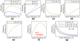
Figure 1: (a) A typical trend of $\mathcal{R}_{k}\left(\mathcal{S},T\right)$ with respect to $T$ and $\mathcal{S}$ in a heterogeneous market. (b) A typical trend of $\mathcal{R}\left(s,T\right)$ with respect to $T$ and $s$ in a homogeneous market. (c, d, and e) A typical trend of $U\left(\mathcal{S},T\right)$ with respect to $T$ in a homogeneous market (c) and in a heterogeneous market with high $\rho_{k}$ (c), mid-range $\rho_{k}$ (d) and low $\rho_{k}$ (e). (f) A trend of $U\left(\mathcal{S},T\right)$ which is not possible in any market scenario. (g) A typical trend of $U\left(\mathcal{S},T\right)$ with respect to $\mathcal{S}$. The black and the blue curves corresponds to objective function, $U\left(\left\{1,2,3\right\},T\right)$, if bid correlation coefficient of operator $3$ is $\rho_{3}^{l}$ and $\rho_{3}^{h}$ respectively where $\rho_{3}^{h}>\rho_{3}^{l}$.

According to Property 2, the revenue function decreases as the set of interested operators $\mathcal{S}$ grows. This is shown in Figure 1.a and 1.b where the blue curve is below the green curve. As $\mathcal{S}$ grows, an operator competes with more operators to get a channel. Hence, the probability of an operator being allocated a channel decreases which in turn decreases its revenue function. We have verified Property 2 numerically.

According to Property 3, the objective function $U\left(\mathcal{S},T\right)$ is unimodal in $T$ with a minimum or it is monotonic increasing in $T$. This happens because of two competing causes. First, as lease duration increases, the regulator is allocating the channels to the operators with the best spectrum utilization less often. This reduces the efficiency of spectrum allocation and hence spectrum utilization decreases. Second, due to bidding inaccuracy an operator may place a lower bid and hence not allocated a channel even though it has a high net revenue in an epoch (and hence a higher spectrum utilization). The chances of such inefficient spectrum allocation increases as lease duration decreases because spectrum auctions occurs more frequently and hence more the chances of such erroneous spectrum allocation. As bidding coefficient $\rho_{k}$ decreases, the bidding inaccuracy increases making the second cause more dominating than the first one. Therefore, the objective function is monotonic non-increasing (special case of unimodal function with minimum at infinity) in $T$ if $\rho_{k}$ is high (Figure 1.c), unimodal in $T$ with a minimum if $\rho_{k}$ is mid-range (Figure 1.d) and monotonic non-decreasing in $T$ if $\rho_{k}$ is low (Figure 1.e). However, the objective function will never be unimodal in $T$ with a maximum (Figure 1.f). For a heterogeneous market, we could only verify Property 3 numerically. But for a homogeneous market, we could rigorously prove that objective function $U\left(s,T\right)$ is monotonic decreasing in $T$ (Figure 1.c) for any value of $\rho_{k}$. Please refer to Appendix D for the proof.

Property 4 discusses the effect of a set of interested operators on objective function and how it changes with bid correlation coefficient. According to Property 4, as $\rho_{a}\rightarrow 1$, $U\left(\mathcal{S}\bigcup\left\{a\right\},T\right)\geq U\left(\mathcal{S},T\right)$; but as $\rho_{a}$ decreases, $U\left(\mathcal{S}\bigcup\left\{a\right\},T\right)$ decreases as well. According to our model, market competition increases as the set of interested operators grows from $\mathcal{S}$ to $\mathcal{S}\bigcup\left\{a\right\}$. Qualitatively, property 4 states that increasing market competition may have two outcomes: (a) Increase in spectrum utilization if bid correlation is high: as $\rho_{a}\rightarrow 1$, there is a value of $\rho_{a}$ above which $U\left(\mathcal{S}\bigcup\left\{a\right\},T\right)\geq U\left(\mathcal{S},T\right)$ implying that the increase in competition due to addition of operator $a$ lead to an increase in spectrum utilization. This is shown in Figure 1.g where the blue curve is above the green curve. (b) Decrease in spectrum utilization if bid correlation is low: as $\rho_{a}$ decreases, the bid of operator $a$ is not a good estimate of its true net revenue which in turn is proportional to operator $a$’s spectrum utilization. Therefore, with decrease in $\rho_{a}$, there is a higher probability of erroneous spectrum allocation to operator $a$ when its spectrum utilization is low. In other words, spectrum allocation becomes less efficient with decrease in $\rho_{a}$ which in turn decreases objective function $U\left(\mathcal{S}\bigcup\left\{a\right\},T\right)$. In some cases, the decrease in spectrum utilization may be large enough that $U\left(\mathcal{S}\bigcup\left\{a\right\},T\right)<U\left(\mathcal{S},T\right)$. This is non-intuitive as it suggests that increasing market competition may not necessarily improve spectrum utilization. This is shown in Figure 1.g where the black curve is below the green curve. For a heterogeneous market, we could only verify Property 4 numerically. But for a homogeneous market, we could rigorously prove that objective function $U\left(s,T\right)$ is monotonic increasing in $s$ for any value of $\rho_{k}$. Please refer to Appendix D for the proof.

We end this section by stressing that the results in the subsequent sections remain valid as long as Properties 1-3 hold. We believe that these properties are robust and hold under various generalizations of our system model. Two such generalizations are as follows. First, we can relax our system model such that an operator can be allocated more than one channel. Second, we can generalize the revenue process given by (1) to other stochastic processes. An interesting generalization is to consider cross-correlation among operators’ revenue processes. Such generalizations may not guarantee closed-form expressions of the revenue function, in which case, it can be estimated using Monte-Carlo simulations.

III Stackelberg Game Formulation and Solution

In this section, we formulate the problem as a Stackelberg game in in Section III-A. We solve Stage-2 of the Stackelberg game and use the result to formulate Stage-1 of the Stackelberg game as an optimization problem $OP1$. We then design algorithms to solve $OP1$ for two market settings: (a) homogeneous market with complete information in Section III-B (Proposition 3), and (b) heterogeneous market with incomplete information in Section III-C (Algorithm 1).

III-A Stackelberg game formulation

In this section, we formulate the optimization problem from the regulator’s and the operators’ perspective. The optimization problem manifests itself in the form of a two-stage Stackelberg game. In Stage-1, the regulator sets the lease duration to maximize spectrum utilization. The payoff of an operator depends on the lease duration. In Stage-2, the operators decide whether to join the market or not depending on the decision which maximizes its payoff. To make decisions the regulator needs information about the operators and the operators need information about other operators in the market. The $k^{th}$ operator can be completely characterized by six parameters which can be represented using the tuple $\xi_{k}=\left(\mu_{k},\sigma_{k},a_{k},\rho_{k},\lambda_{k},\Lambda_{k}\right)$. Only the $k^{th}$ operator knows the true value of these six parameters. To model incomplete information games, we assume the regulator and other operators in the market only has a point estimate of the $k^{th}$ operator’s parameters [34]. Let the estimate be $\widehat{\xi}_{k}=\left(\widehat{\mu}_{k},\widehat{\sigma}_{k},\widehat{a}_{k},\widehat{\rho}_{k},\widehat{\lambda}_{k},\widehat{\Lambda}_{k}\right)$. Please note that for simplicity, we have assumed that the entire market has one common estimate of $k^{th}$ operator’s parameters. This can be easily generalized where the regulator and the operators have different estimates of $k^{th}$ operator’s parameters.

Stackelberg equilibrium of a Stackelberg game can be found using backward induction [35]. To apply backward induction, we start with Stage-2 and analyze the operators’ decision strategy given a lease duration. Then we solve for Stage-1 where the regulator decides the lease duration knowing the possible response of the operators to the lease duration. Consider Stage-2 of the game, also referred as the subgame. The outcome of this process is the function $\mathcal{S}\left(T\right)$ which characterizes the set of interested operators as a function of lease duration $T$. An operators decision to enter the market depends on its revenue function $\mathcal{R}_{k}\left(\mathcal{S},T\right)$. $\mathcal{R}_{k}\left(\mathcal{S},T\right)$ is the true revenue function of the $k^{th}$ operator. To compute $\mathcal{R}_{k}\left(\mathcal{S},T\right)$, the $k^{th}$ operator needs to know $\xi_{j}$ of all the operators in the market which it does not. Let $\widehat{\mathcal{R}}_{k}\left(\mathcal{S},T\right)$ denotes the revenue function of the $k^{th}$ operator as perceived by the $k^{th}$ operator due to incomplete information scenario. To compute $\widehat{\mathcal{R}}_{k}\left(\mathcal{S},T\right)$, the $k^{th}$ operator uses its true parameters $\xi_{k}$ and estimates $\widehat{\xi}_{j}$, where $j\neq k$, of other operator’s parameters. If $T>\Lambda_{k}$, then the $k^{th}$ operator will definitely not enter the market. If $T\leq\Lambda_{k}$, then the payoff of the $k^{th}$ operator is

$$\pi_{k}\left(\mathcal{X}\right)=\widehat{\mathcal{R}}_{k}\left(\mathcal{X},T\right)-\lambda_{k}$$ (15)

if it enters the market where $\mathcal{X}$ is the set of operators who decided to enter the market and $k\in\mathcal{X}$. Payoff of the $k^{th}$ operator is $0$ if it does not enter the market. With (15) as the payoff function, the subgame can have multiple pure strategy Nash equilibria. For example, consider a complete information game which is a subset of incomplete information game with $\widehat{\xi}_{k}=\xi_{k}\,;\,\forall k$. There is $M=1$ channel and $N=2$ operators. Parameters $\xi_{k}$ of these operators are $\mu_{k}=\mu\,,\,\lambda_{k}=\lambda\,,\,\Lambda_{k}=\infty\,;\,k=1,2$. If the lease duration $T=\frac{\lambda}{\mu}$, then $\widehat{\mathcal{R}}_{k}\left(\left\{k\right\},T\right)=\mu T=\lambda\,;\,k=1,2$ and $\widehat{\mathcal{R}}_{k}\left(\left\{1,2\right\},T\right)<\mu T=\lambda\,;\,k=1,2$ (due to Property 2). Hence, there are two pure strategy Nash equilibria; Operator $1$ enters the market while Operator $2$ does not and vice-versa.

If the subgame has multiple pure strategy Nash equilibria, then Stage-1 will have multiple optimal solutions for lease duration each corresponding to one of the NE of Stage-1. In other words, for a given set of market parameters, there can be multiple optimal lease durations. In order to simplify the analysis, we consider a setting where the subgame has a unique pure strategy NE. In one such setting, an operator is interested in maximizing its minimum payoff. The obtained NE is called Max-Min NE and has been considered in previous works like [36]. According to Property 2, payoff decreases as the set $\mathcal{X}$ increases. So the minimum payoff corresponds to the largest $\mathcal{X}$. The largest $\mathcal{X}$ is composed of those operators who may join the market. The $k^{th}$ operator will definitely not join the market if either $T>\Lambda_{k}$ or $\mu_{k}T<\lambda_{k}$. The inequality $T>\Lambda_{k}$ is obvious. To appreciate the inequality $\mu_{k}T<\lambda_{k}$, note that the maximum payoff of the $k^{th}$ operator is $\mu_{k}T-\lambda_{k}$ which happens when it is alone in the market, i.e. $\mathcal{X}=\left\{k\right\}$ and hence $\widehat{\mathcal{R}}_{k}\left(\left\{k\right\},T\right)=\mu_{k}T$ . This is due to Property 2. If $\mu_{k}T<\lambda_{k}$, then the payoff of the $k^{th}$ operator is negative if it enters the market, irrespective of the decision of other operators. Hence, its dominant strategy is not to enter the market. To conclude, the $k^{th}$ operator may join the market if and only if $T\leq\Lambda_{k}$ and $\mu_{k}T\geq\lambda_{k}$. But the $k^{th}$ operator does not know the true value of $\mu_{j}$, $\lambda_{j}$ and $\Lambda_{j}$ if $j\neq k$. Therefore, the largest set of interested operators who may join the market, according to the $k^{th}$ operator, for lease duration $T$ is

$$\mathcal{S}_{k}^{L}\left(T\right) = \left\{\vphantom{\widehat{\Lambda}_{j}}j\>:\>j=k\,,\,T\leq\Lambda_{j}\,,\,\mu_{j}T\geq\lambda_{j}\quad\text{{or}}\right.$$ (16)

$$\left.\qquad\>j\neq k\,,\,T\leq\widehat{\Lambda}_{j}\,,\,\widehat{\mu}_{j}T\geq\widehat{\lambda}_{j}\right\}$$

To this end we can conclude that according to the $k^{th}$ operator, its minimum payoff is $\widehat{\mathcal{R}}_{k}\left(\mathcal{S}_{k}^{L}\left(T\right),T\right)-\lambda_{k}$. This leads to the following proposition.

Proposition 2.

The subgame has a unique Max-Min Nash equilibrium which is given by the set of interested operators

$$\mathcal{S}\left(T\right)=\left\{k\>:\>T\leq\Lambda_{k}\,,\,\widehat{\mathcal{R}}_{k}\left(\mathcal{S}_{k}^{L}\left(T\right),T\right)\geq\lambda_{k}\right\}$$ (17)

Equation 17 is the solution (true) of the subgame. With slight abuse of notation let

$$U\left(T\right)=U\left(\mathcal{S}\left(T\right),T\right)$$ (18)

$U\left(T\right)$ is the true objective function because it depends on the true solution of the subgame, $\mathcal{S}\left(T\right)$, and also because computation of $U\left(\mathcal{S},T\right)$ is based only on the true parameters $\xi_{j}$. In Stage-1, the regulator wants to maximize $U\left(T\right)$. Hence, to calculate $U\left(T\right)$, the regulator needs to know $\xi_{j}$ of all the operators. But the regulator does not know $\xi_{j}$ of any operator; it only knows the estimates $\widehat{\xi}_{j}$. Let $\widetilde{\mathcal{R}}_{k}\left(\mathcal{S},T\right)$ and $\widetilde{U}\left(\mathcal{S},T\right)=\frac{1}{T}\underset{k\in S}{\sum}\widetilde{\mathcal{R}}_{k}\left(S,T\right)$ denote the revenue function of the $k^{th}$ operator and the objective function as perceived by the regulator respectively. Unlike $\widehat{\mathcal{R}}_{k}\left(\mathcal{S},T\right)$, $\widetilde{\mathcal{R}}_{k}\left(\mathcal{S},T\right)$ is calculated only based on estimates $\widehat{\xi}_{j}$. The largest set of interested operators as perceived by the regulator, $\widetilde{\mathcal{S}}^{L}\left(T\right)$, and the perceived set of interested operators, $\widetilde{S}\left(T\right)$, is given by

$$\widetilde{\mathcal{S}}^{L}\left(T\right)=\left\{k\,:\,T\leq\widehat{\Lambda}_{k}\,,\,\widehat{\mu}_{k}T\geq\widehat{\lambda}_{k}\right\}$$ (19)

$$\widetilde{S}\left(T\right)=\left\{k\,:\,T\leq\widehat{\Lambda}_{k}\,,\,\widetilde{\mathcal{R}}_{k}\left(\widetilde{\mathcal{S}}^{L}\left(T\right),T\right)\geq\widehat{\lambda}_{k}\right\}$$ (20)

Note that $\widetilde{\mathcal{S}}\left(T\right)\subseteq\widetilde{\mathcal{S}}^{L}\left(T\right)$ because $\widetilde{\mathcal{R}}_{k}\left(\widetilde{\mathcal{S}}^{L}\left(T\right),T\right)\leq\widetilde{\mathcal{R}}_{k}\left(\left\{k\right\},T\right)=\widehat{\mu}_{k}T$ (Property 2). With slight abuse of notation let $\widetilde{U}\left(T\right)=\widetilde{U}\left(\widetilde{\mathcal{S}}\left(T\right),T\right)$ be the perceived objective function. In Stage-1, the regulator solves the following optimization problem

$$OP1\begin{cases}\underset{T\in\mathbb{Z}^{+}}{\max}\quad\widetilde{U}\left(T\right)=\widetilde{U}\left(\widetilde{\mathcal{S}}\left(T\right),T\right)\end{cases}$$

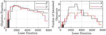
Figure 2: A typical plot of objective function (true) $U\left(T\right)$, perceived objective function $\widetilde{U}\left(T\right)$, number of interested operators (true) $s\left(T\right)=\left|\mathcal{S}\left(T\right)\right|$, and the perceived number of interested operators $\widetilde{s}\left(T\right)=\left|\widetilde{\mathcal{S}}\left(T\right)\right|$. For this plot, $N=10$ , $M=2$ and the true parameters $\xi_{k}$ are chosen uniformly at random. The estimated parameters $\widehat{\xi}_{k}$ are chosen uniformly at random such that they are within $\pm 25\%$ of the true parameters.

The regulator chooses lease duration $T$ to maximize the perceived objective function $\widetilde{U}\left(T\right)$. The perceived objective function and the objective function (true) $U\left(T\right)$ may not be equal as shown in Figure 2. Therefore, a lease duration which maximizes the perceived objective function may not maximize the objective function. This leads to sub-optimal spectrum utilization due to incomplete information games.

The perceived set of interested operators, $\widetilde{\mathcal{S}}\left(T\right)$, can be implicitly controlled by choosing a suitable $T$. A significant part of solving $OP1$ is to find an $\widetilde{\mathcal{S}}\left(T\right)$ that maximizes $\widetilde{U}\left(T\right)$. The number of combinations of $\widetilde{\mathcal{S}}\left(T\right)$ can be exponential in $N$. Therefore, $OP1$ is reminiscent of combinatorial optimization which makes it difficult to solve even though it is a scalar optimization problem in $T$. A typical plot of objective function $\widetilde{U}\left(T\right)$ and the perceived number of interested operators $\widetilde{s}\left(T\right)=\left|\widetilde{\mathcal{S}}\left(T\right)\right|$ is shown in Figure 2 (black curve). The discontinuous and non-smooth nature of $\widetilde{U}\left(T\right)$ is another reason why it is difficult to solve $OP1$.

Figure 2 also shows that the optimal lease duration is non-trivial. If the lease duration is too low, MER of many operators are not satisfied (Property 1) and hence $\widetilde{\mathcal{S}}\left(T\right)$ is small. Therefore, $\widetilde{U}\left(T\right)$ is low (high) according to Property 4 if bid correlation if high (low). If the lease duration is too high and bid correlation is high (low), $\widetilde{U}\left(T\right)$ is low (high) for one of the two reasons. First, due to Property 3. This is because the objective function is monotonic decreasing (increasing) in lease duration if bid correlation is high (low). Second, $\widetilde{\mathcal{S}}\left(T\right)$ is small either because the operators cannot afford a channel with long lease duration or because the revenue function decreases for a higher value of lease duration as suggested by Property 1. Hence, the optimal lease duration is neither too high nor too low as shown in Figure 2.

III-B Stackelberg game solution: Homogeneous Market with Complete Information

For complete information games, $\widehat{\xi}_{k}=\xi_{k}\,;\,\forall k$, and for homogeneous market, $\xi_{k}=\xi\,;\,\forall k$. Let, $\xi=\left(\mu,\sigma,a,\rho,\lambda,\Lambda\right)$. Since $\widehat{\xi}_{k}=\xi_{k}$, the revenue function of the $k^{th}$ operator as perceived by the $k^{th}$ operator, $\widehat{\mathcal{R}}_{k}\left(\mathcal{S},T\right)$, and as perceived by the regulator ,$\widetilde{\mathcal{R}}_{k}\left(\mathcal{S},T\right)$, are equal to the revenue function (true) $\mathcal{R}_{k}\left(\mathcal{S},T\right)$. Similarly, the perceived objective function, $\widetilde{U}\left(T\right)$, is equal to the objective function (true), $U\left(T\right)$. Also, since the market is homogeneous in $\xi_{k}$, the revenue is same for all the operators, i.e. $\mathcal{R}_{k}\left(\mathcal{S},T\right)=\mathcal{R}\left(s,T\right)\,;\,\forall k$. The following proposition can be used to calculate the optimal lease duration, $T^{*}$, and the optimal value of the objective function, $U^{*}$, for a homogeneous market with complete information.

Proposition 3.

Let $\theta$ be the solution to $\mathcal{R}\left(N,\theta\right)=\lambda$ and $\left\lceil\cdot\right\rceil$ be the ceiling function. If $\left\lceil\theta\right\rceil\leq\Lambda$, then $T^{*}=\left\lceil\theta\right\rceil$ and $U^{*}=\frac{N}{\left\lceil\theta\right\rceil}\mathcal{R}\left(N,\left\lceil\theta\right\rceil\right)$. However, if $\left\lceil\theta\right\rceil>\Lambda$, then $U^{*}=0$ and $T^{*}$ can be set to any value.

Proof:

Please refer to Appendix E for the proof. ∎

Intuitively, Proposition 3 can be understood as follows. In a homogeneous market, either all or none of the operators are interested in joining the market. If none of the operators are interested in joining the market, then the objective function is zero which is trivial. Hence, to have $U^{*}>0$, $T^{*}$ should be such that all the operators are interested in joining the market. If all the $N$ operators join the market, then the revenue function of an operator is $\mathcal{R}\left(N,T^{*}\right)$. Also, for operators to be interested in joining the market, $T^{*}$ must also satisfy $\mathcal{R}\left(N,T^{*}\right)\geq\lambda$ and $T^{*}\leq\Lambda$ (refer to (20)). As discussed in Section II-C, the revenue function of a homogeneous market is monotonic increasing in lease duration. Hence, the solution to $\mathcal{R}\left(N,T^{*}\right)\geq\lambda$ is $T^{*}\geq\left\lceil\theta\right\rceil$ where $\theta$ if the solution to $\mathcal{R}\left(N,\theta\right)=\lambda$. The ceiling function $\left\lceil\cdot\right\rceil$ is needed because we consider a time slotted model. To this end we conclude that, $U^{*}>0$ if and only if $T^{*}$ satisfies $\left\lceil\theta\right\rceil\leq T^{*}\leq\Lambda$. If $\left\lceil\theta\right\rceil>\Lambda$, then there does not exists a $T^{*}$ that satisfies $\left\lceil\theta\right\rceil\leq T^{*}\leq\Lambda$. Hence, $U^{*}=0$ and $T^{*}$ can be set to any value. If $\left\lceil\theta\right\rceil\leq\Lambda$, then $T^{*}=\left\lceil\theta\right\rceil$ maximizes the objective function because for a homogeneous market, objective function is monotonic decreasing in lease duration (refer to Section II-C). For $T^{*}=\left\lceil\theta\right\rceil$, all the operators are interested in joining the market. Hence, according to (14), $U^{*}=\frac{N}{\left\lceil\theta\right\rceil}\mathcal{R}\left(N,\left\lceil\theta\right\rceil\right)$. This completes the explanation of Proposition 3.

Finally, to solve $OP1$ for a homogeneous market with complete information, we have to compute $\theta$. Since, $\mathcal{R}\left(N,\theta\right)$ is monotonic increasing in $\theta$, the equation $\mathcal{R}\left(N,\theta\right)=\lambda$ can be solved using binary search or Newton-Raphson method.

III-C Stackelberg game solution: Heterogeneous Market with Incomplete Information

1

2

Input: $N$, $M$, $\widehat{\xi}_{k}\,;\,k=1,\ldots,N$

3

Output: $\widetilde{T}^{*}$, $\widetilde{U}^{*}$, $\widetilde{\mathcal{S}}^{*}$

4

5Initialize an empty list $Q^{L}$ whose elements are ordered pairs $\left(T,k\right)$ where $T$ denotes lease duration and $k$ denotes operator index

6

7for $k\leftarrow 1$ to $N$ do

8      Append $\left(\left\lceil\frac{\widehat{\lambda}_{k}}{\widehat{\mu}_{k}}\right\rceil,k\right)$ and $\left(\widehat{\Lambda}_{k}+1,k\right)$ onto $Q^{L}$

9     

10Sort $Q^{L}$ in ascending order of lease duration

11

12Set $\widetilde{U}^{*}=0$ and $\mathcal{X}^{L}_{0}=\emptyset$

13

14for $i\leftarrow 1$ to $\left|Q^{L}\right|$ do

15     

16     if $Q^{L}_{i}.k\in\mathcal{X}^{L}_{i-1}$ then set $\mathcal{X}^{L}_{i}=\mathcal{X}^{L}_{i-1}-\left\{Q^{L}_{i}.k\right\}$; else set $\mathcal{X}^{L}_{i}=\mathcal{X}^{L}_{i-1}\bigcup\left\{Q^{L}_{i}.k\right\}$

17     

18     if $Q^{L}_{i}.T<Q^{L}_{i+1}.T$ or $i=\left|Q^{L}\right|$ then

19          

20          $\mathcal{X}_{i}^{L}$ is one of the sets in $\mathcal{F}^{L}$. Set $\theta_{i}^{L}=Q^{L}_{i}.T$ and $\Theta_{i}^{L}=Q^{L}_{i+1}.T-1$

21          

22          Initialize an empty list $Q$ whose elements are ordered pairs $\left(T,k\right)$ where $T$ denotes lease duration and $k$ denotes operator index

23          

24          for $k$ in $\mathcal{X}^{L}_{i}$ do

25                Find $\gamma_{k}$ and $\Gamma_{k}$, the minimum and the maximum lease duration resp. in the interval $\left[\theta_{i}^{L},\Theta_{i}^{L}\right]$ s.t. $\widetilde{\mathcal{R}}_{k}\left(\mathcal{X}_{i}^{L},T\right)\geq\widehat{\lambda}_{k}\,;\,\forall T\in\left[\gamma_{k},\Gamma_{k}\right]$

26               

27               if $\gamma_{k}$ and $\Gamma_{k}$ exists then

28                     Append $\left(\gamma_{k},k\right)$ onto $Q$

29                    if $\Gamma_{k}<\Theta_{i}^{L}$ then append $\left(\Gamma_{k}+1,k\right)$ onto $Q$

30          Sort $Q$ in ascending order of lease duration

31          

32          Set $\mathcal{X}_{0}=\emptyset$

33          

34          for $j\leftarrow 1$ to $\left|Q\right|$ do

35               

36               if $Q_{j}.k\in\mathcal{X}_{j-1}$ then set $\mathcal{X}_{j}=\mathcal{X}_{j-1}-\left\{Q_{j}.k\right\}$; else set $\mathcal{X}_{j}=\mathcal{X}_{j-1}\bigcup\left\{Q_{j}.k\right\}$

37               

38               if ($Q_{j}.T<Q_{j+1}.T$ or $j=\left|Q\right|$) then

39                    

40                    $\mathcal{X}_{j}$ is one of the sets in $\mathcal{F}$. Set $\theta_{j}=Q_{j}.T$ and $\Theta_{j}=Q_{j+1}.T-1$

41                    

42                    if $\widetilde{U}\left(\mathcal{X}_{j}\,,\,\theta_{j}\right)>\widetilde{U}^{*}$ then

43                          Set $\widetilde{T}^{*}=\theta_{j}$ , $\widetilde{U}^{*}=\widetilde{U}\left(\mathcal{X}_{j}\,,\,\theta_{j}\right)$ , $\widetilde{\mathcal{S}}^{*}=\mathcal{X}_{j}$

44                         

45                    if $\widetilde{U}\left(\mathcal{X}_{j}\,,\,\Theta_{j}\right)>\widetilde{U}^{*}$ then

46                          Set $\widetilde{T}^{*}=\Theta_{j}$ , $\widetilde{U}^{*}=\widetilde{U}\left(\mathcal{X}_{j}\,,\,\Theta_{j}\right)$ , $\widetilde{\mathcal{S}}^{*}=\mathcal{X}_{j}$

47                         

Algorithm 1 Optimization algorithm to solve $OP1$ for a heterogeneous market with incomplete information

Algorithm 1 is a psuedocode to solve $OP1$ for a heterogeneous market with incomplete information. Proposition 3 which solves $OP1$ for a homogeneous market with complete information is a special case of Algorithm 1. The main difficulty about solving $OP1$ is the change in $\widetilde{\mathcal{S}}\left(T\right)$ with change in $T$. This leads to discontinuities in the objective function of $OP1$. Algorithm 1 solves this issue by dividing the entire positive real axis which represents the lease duration into intervals such that $\widetilde{\mathcal{S}}\left(T\right)$ does not change within these intervals. The optimal lease duration within these intervals will lie in its boundaries because of Property 3. Finally, the optimal lease duration can be found by comparing the maximum lease duration within each of these intervals. In the rest of this section, we will device an efficient approach to find these intervals. We will approach this in steps. First, we will convert $OP1$ into a combinatorial optimization problem $OP2$. By doing so, we formalize the idea discussed in this paragraph. Second, we will discuss how to divide the entire positive real axis into intervals such that $\widetilde{\mathcal{S}}^{L}\left(T\right)$ does not change within these intervals. This is required because $\widetilde{\mathcal{S}}\left(T\right)$ is a function of $\widetilde{\mathcal{S}}^{L}\left(T\right)$ (refer to (20)). Therefore, to find the intervals corresponding to $\widetilde{\mathcal{S}}\left(T\right)$, we have to first find the intervals corresponding to $\widetilde{\mathcal{S}}^{L}\left(T\right)$. The process of finding the intervals corresponding to $\widetilde{\mathcal{S}}^{L}\left(T\right)$ will be exemplified using Example 1, Example 2 and Figure 3. Finally, we discuss how to find the intervals corresponding to $\widetilde{\mathcal{S}}\left(T\right)$ which is very similar to finding the intervals corresponding to $\widetilde{\mathcal{S}}^{L}\left(T\right)$.

Let $\mathcal{F}$ be a family of sets containing all possible perceived sets of interested operators. Mathematically, $\mathcal{F}=\left\{\overline{\mathcal{S}}\>:\>\left(\exists\,T\in\mathbb{Z}^{+}\right)\left[\widetilde{\mathcal{S}}\left(T\right)=\overline{\mathcal{S}}\right]\right\}$. For a given $\overline{\mathcal{S}}\in\mathcal{F}$, there can be several values of $T$ satisfying $\widetilde{\mathcal{S}}\left(T\right)=\overline{\mathcal{S}}$. Let $T_{m}\left(\overline{\mathcal{S}}\right)$ and $T_{M}\left(\overline{\mathcal{S}}\right)$ denote the minimum and the maximum $T$ respectively satisfying $\widetilde{\mathcal{S}}\left(T\right)=\overline{\mathcal{S}}$. According to Property 3, either $T_{m}\left(\overline{\mathcal{S}}\right)$ or $T_{M}\left(\overline{\mathcal{S}}\right)$ maximizes $OP1$ if $\widetilde{\mathcal{S}}\left(T\right)=\overline{\mathcal{S}}$. Based on this discussion, $OP1$ is equivalent to the following optimization problem

$$OP2\begin{cases}\underset{\overline{\mathcal{S}}\in\mathcal{F}}{\max}\;\widetilde{U}\left(\overline{\mathcal{S}}\right)=\max\left(\widetilde{U}\left(\overline{\mathcal{S}},T_{m}\left(\overline{\mathcal{S}}\right)\right),\widetilde{U}\left(\overline{\mathcal{S}},T_{M}\left(\overline{\mathcal{S}}\right)\right)\right)\end{cases}$$

$OP2$ is a combinatorial optimization problem in $\overline{\mathcal{S}}$. Let $\widetilde{T}^{*}$ be the optimal solution of $OP1$. If $\widetilde{\mathcal{S}}^{*}$ is an optimal solution of $OP2$, then $\widetilde{T}^{*}$ is either $T_{m}\left(\widetilde{\mathcal{S}}^{*}\right)$ or $T_{M}\left(\widetilde{\mathcal{S}}^{*}\right)$, whichever maximizes $\widetilde{U}\left(\widetilde{\mathcal{S}}^{*},T\right)$. In Algorithm 1, we find $\widetilde{\mathcal{S}}^{*}$ (and hence $\widetilde{T}^{*}$) by iterating over all $\overline{\mathcal{S}}\in\mathcal{F}$ to find the one which maximizes $\widetilde{U}\left(\overline{\mathcal{S}}\right)$. To do so, we need a constructive method to find all the sets in $\mathcal{F}$. In the rest of the section, we discuss the steps involved in finding all the sets in $\mathcal{F}$ and the corresponding line number of Algorithm 1 which implements that step. One of the outputs of Algorithm 1 is $\widetilde{U}^{*}$, the optimal value of the perceived objective function. But the value of the objective function (true) corresponding to optimal solution of $OP1$, $\widetilde{T}^{*}$, is given by (18) and is equal to

$$U^{*}=U\left(\mathcal{S}\left(\widetilde{T}^{*}\right),\widetilde{T}^{*}\right)$$ (21)

In order to find all the sets in $\mathcal{F}$, we have to first find all the sets in $\mathcal{F}^{L}=\left\{\overline{\mathcal{S}}\>:\>\left(\exists\,T\in\mathbb{Z}^{+}\right)\left[\widetilde{\mathcal{S}}^{L}\left(T\right)=\overline{\mathcal{S}}\right]\right\}$. $\mathcal{F}^{L}$ is a family of sets containing all possible largest sets of interested operators as perceived by the regulator. According to (19), $k\in\widetilde{\mathcal{S}}^{L}\left(T\right)$ if and only if $T\geq\left\lceil\frac{\widehat{\lambda}_{k}}{\widehat{\mu}_{k}}\right\rceil$ and $T<\widehat{\Lambda}_{k}+1$. The ceiling function $\left\lceil\cdot\right\rceil$ is needed because we consider a time slotted model. Consider the ordered pairs $\left(\left\lceil\frac{\widehat{\lambda}_{k}}{\widehat{\mu}_{k}}\right\rceil,k\right)$ and $\left(\widehat{\Lambda}_{k}+1,k\right)$ where the first element is lease duration and the second element is operator index. A list $Q^{L}$ contains such ordered pairs corresponding to all the $N$ operators (line 1-3). The size of $Q^{L}$ is $\left|Q^{L}\right|=2N$ as there are $2$ ordered pairs corresponding to each of the $N$ operators. Let $Q_{i}^{L}$ be the $i^{th}$ element of $Q^{L}$. We use the dot ($\cdot$) operator to access the lease duration and the operator index of the elements of $Q^{L}$. In other words, $Q_{i}^{L}.T$ and $Q_{i}^{L}.k$ denote the lease duration and the operator index respectively corresponding to ordered pair $Q_{i}^{L}$. All the sets in $\mathcal{F}^{L}$ can be found using the following steps:

1. Sort $Q^{L}$ in ascending order of lease duration (line 4). Traverse the sorted list $Q^{L}$ from $i=1$ to $\left|Q^{L}\right|$ and repeat steps (A2) to (A4) in every iteration (line 6). Let $\mathcal{X}_{i}^{L}$ be the largest set of interested operators as perceived by the regulator which is obtained in the $i^{th}$ iteration. Set $\mathcal{X}_{0}^{L}=\emptyset$ (line 5). Let $i$ be the current iteration.

2. If the operator with index $Q_{i}^{L}.k$ is not in set $\mathcal{X}_{i-1}^{L}$, add $Q_{i}^{L}.k$ to $\mathcal{X}_{i-1}^{L}$ to get $\mathcal{X}_{i}^{L}$. Else if the operator with index $Q_{i}^{L}.k$ is in set $\mathcal{X}_{i-1}^{L}$, remove $Q_{i}^{L}.k$ from $\mathcal{X}_{i-1}^{L}$ to get $\mathcal{X}_{i}^{L}$. This is implemented in line 7.

3. If $Q_{i}^{L}.T<Q_{i+1}^{L}.T$ or $i=\left|Q^{L}\right|$, then the obtained $\mathcal{X}_{i}^{L}$ in step (A2) is one of the sets in $\mathcal{F}^{L}$. $\widetilde{\mathcal{S}}^{L}\left(T\right)=\mathcal{X}_{i}^{L}$ for all $T\in\left[Q_{i}^{L}.T\,,\,Q_{i+1}^{L}.T-1\right]$.

4. If $Q_{i}^{L}.T=Q_{i+1}^{L}.T$, then the obtained $\mathcal{X}_{i}^{L}$ in step (A2) is not one of the sets in $\mathcal{F}^{L}$. This is because operators $Q_{i}^{L}.k$ and $Q_{i+1}^{L}.k$ corresponding to ordered pairs $Q_{i}^{L}$ and $Q_{i+1}^{L}$ respectively must update $\mathcal{X}_{i-1}^{L}$ simultaneously as both these ordered pairs have the same lease duration.

The if statement in line 8 implements steps (A3) and (A4). If $Q_{i}^{L}.T=Q_{i+1}^{L}.T$, then the if statement in line 8 is false and the algorithm simply loops to the next iteration without considering the obtained $\mathcal{X}_{i}^{L}$ in line 7 as one of the sets in $\mathcal{F}^{L}$. The following examples exemplifies the working of steps (A1) to (A4).

Example 1.

Consider $N=3$ operators with $\widehat{\mu}_{k}=1\,;\,\forall k$, $\widehat{\lambda}_{k}$’s are $\left[175,100,200\right]$ and $\widehat{\Lambda}_{k}$’s are $\left[300,450,625\right]$. The sorted list $Q^{L}$ for this example is shown in Figure 3.a. As we traverse Figure 3.a from left to right, $\widetilde{\mathcal{S}}^{L}\left(T\right)$ is $\emptyset$ if $T\leq 99$, $\left\{2\right\}$ if $T\in\left[100,174\right]$, $\left\{1,2\right\}$ if $T\in\left[175,199\right]$, $\left\{1,2,3\right\}$ if $T\in\left[200,299\right]$, $\left\{2,3\right\}$ if $T\in\left[300,449\right]$, $\left\{3\right\}$ if $T\in\left[450,624\right]$ and $\emptyset$ if $T\geq 625$. Hence, $\mathcal{F}^{L}$ consists of the sets $\left\{2\right\}$, $\left\{1,2\right\}$, $\left\{1,2,3\right\}$, $\left\{2,3\right\}$, $\left\{3\right\}$, and $\emptyset$.

Example 2.

This example demonstrates the importance of step (A4) by considering mutiple ordered pairs with same lease duration. The setting is the same as Example 1 except that $\widehat{\lambda}_{k}$’s are $\left[200,100,200\right]$. The sorted list $Q^{L}$ for this example is shown in Figure 3.b. As we traverse Figure 3.b from left to right, $\widetilde{\mathcal{S}}^{L}\left(T\right)$ is $\emptyset$ if $T\leq 99$, $\left\{2\right\}$ if $T\in\left[100,199\right]$, $\left\{1,2,3\right\}$ if $T\in\left[200,299\right]$, $\left\{2,3\right\}$ if $T\in\left[300,449\right]$, $\left\{3\right\}$ if $T\in\left[450,624\right]$ and $\emptyset$ if $T\geq 625$. Hence, $\mathcal{F}^{L}$ consists of the sets $\left\{2\right\}$, $\left\{1,2,3\right\}$, $\left\{2,3\right\}$, $\left\{3\right\}$, and $\emptyset$. Unlike Example 1, $\left\{1,2\right\}\notin\mathcal{F}^{L}$ since ordered pairs $\left(200,1\right)$ and $\left(200,3\right)$ have the same lease duration.

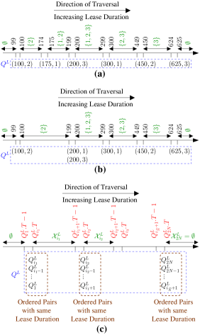
Figure 3: (a) Figure showing sorted list $Q^{L}$ (in blue) and the sets in $\mathcal{F}^{L}$ (in green) for Example 1. (b) Figure showing sorted list $Q^{L}$ (in blue) and the sets in $\mathcal{F}^{L}$ (in green) for Example 2. (c) A generic pictorial representation showing the sorted list $Q^{L}$ (in blue), the sets in $\mathcal{F}^{L}$ (in green) and the interval of lease duration corresponding to the sets in $\mathcal{F}^{L}$ (in red).

Figures 3.a and 3.b show that steps (A1) to (A4) divides the set of positive integers into contiguous intervals of lease duration. Each interval has its corresponding $\mathcal{X}_{i}^{L}$. A general setup is shown in Figure 3.c. Let $i_{1}$, $i_{2}$, $\ldots$ , $2N$, where $i_{1}<i_{2}<\cdots<2N$, denote all the iterations such that $Q_{i}^{L}.T<Q_{i+1}^{L}.T$ (or $i=\left|Q^{L}\right|=2N$). Refering to step (A3), $\mathcal{F}^{L}$ consists of the sets $\mathcal{X}_{i_{1}}^{L}$, $\mathcal{X}_{i_{2}}^{L}$, $\ldots$ , $\mathcal{X}_{2N}^{L}$. Each of these sets are associated with a corresponding interval of lease duration. As shown in Figure 3.c, $\widetilde{\mathcal{S}}^{L}\left(T\right)$ is equal to $\mathcal{X}_{i_{1}}^{L}$ in the interval $\left[Q_{i_{1}}^{L}.T\,,\,Q_{i_{1}+1}^{L}.T-1\right]$, $\mathcal{X}_{i_{2}}^{L}$ in the interval $\left[Q_{i_{2}}^{L}.T\,,\,Q_{i_{2}+1}^{L}.T-1\right]$ etc. These intervals are non-overlapping and their union spans the entire set of positive integers. We want to design an algorithm to find all the sets in $\mathcal{F}$. $\mathcal{F}$ contains all the sets $\widetilde{\mathcal{S}}\left(T\right)$ as $T$ varies in the set of positive integers. This problem is equivalent to finding all the sets $\widetilde{\mathcal{S}}\left(T\right)$ as $T$ varies in each one of these intervals. The equivalence is due to the fact that the union of these intervals spans the entire set of positive integers.

Let $\left[\theta_{i}^{L},\Theta_{i}^{L}\right]$ be one such interval where $Q_{i}^{L}$.T<$Q_{i+1}^{L}$.T, $\theta_{i}^{L}=Q_{i}^{L}.T$, and $\Theta_{i}^{L}=Q_{i+1}^{L}.T-1$ (line 9). We have $\widetilde{\mathcal{S}}^{L}\left(T\right)=\mathcal{X}_{i}^{L}\,;\,\forall T\in\left[\theta_{i}^{L},\Theta_{i}^{L}\right]$. In the interval $\left[\theta_{i}^{L},\Theta_{i}^{L}\right]$, the perceived set of interested operators $\widetilde{\mathcal{S}}\left(T\right)\subseteq\mathcal{X}_{i}^{L}$. If $k\in\mathcal{X}_{i}^{L}$, then $T\leq\widehat{\Lambda}_{k}$ (refer to (19)). Hence, for the interval $\left[\theta_{i}^{L},\Theta_{i}^{L}\right]$, (20) is equivalent to $\widetilde{\mathcal{S}}\left(T\right)=\left\{k\in\mathcal{X}_{i}^{L}\,:\,\widetilde{\mathcal{R}}_{k}\left(\mathcal{X}_{i}^{L},T\right)\geq\widehat{\lambda}_{k}\right\}$. According to Property 1, $\widetilde{\mathcal{R}}_{k}\left(\mathcal{X}_{i}^{L},T\right)$ is unimodal in $T$. Therefore, the solution to $\widetilde{\mathcal{R}}_{k}\left(\mathcal{X}_{i}^{L},T\right)\geq\widehat{\lambda}_{k}$ in the interval $\left[\theta_{i}^{L},\Theta_{i}^{L}\right]$ is also an interval $\left[\gamma_{k},\Gamma_{k}\right]$. $\gamma_{k}$ and $\Gamma_{k}$ are the minimum and the maximum lease duration satisfying $\theta_{i}^{L}\leq\gamma_{k}\leq\Gamma_{k}\leq\Theta_{i}^{L}$ such that $\widetilde{\mathcal{R}}_{k}\left(\mathcal{X}_{i}^{L},T\right)\geq\widehat{\lambda}_{k}\,;\,\forall T\in\left[\gamma_{k},\Gamma_{k}\right]$. If $T\in\left[\theta_{i}^{L},\Theta_{i}^{L}\right]$, there are three possible cases:

1. $\gamma_{k}$ and $\Gamma_{k}$ exist and $\Gamma_{k}<\Theta_{i}^{L}$: One such example is shown in Figure 4.a. In this case, the $k^{th}$ operator is associated with two ordered pairs $\left(\gamma_{k},k\right)$ and $\left(\Gamma_{k}+1,k\right)$ implying that $k\in\widetilde{\mathcal{S}}\left(T\right)$ if and only if $T\geq\gamma_{k}$ and $T<\Gamma_{k}+1$.

2. $\gamma_{k}$ and $\Gamma_{k}$ exist and $\Gamma_{k}=\Theta_{i}^{L}$: One such example is shown in Figure 4.b. In this case, the $k^{th}$ operator is associated with an ordered pair $\left(\gamma_{k},k\right)$ implying that $k\in\widetilde{\mathcal{S}}\left(T\right)$ if and only if $T\geq\gamma_{k}$.

3. $\gamma_{k}$ and $\Gamma_{k}$ do not exist: One such example is shown in Figure 4.c. In this case, the $k^{th}$ operator is not associated with any ordered pair because $k\notin\widetilde{\mathcal{S}}\left(T\right)$ for all $T$.

Consider a list $Q$ containing the ordered pairs associated with all the operators in $\mathcal{X}_{i}^{L}$. List $Q$ is constructed in lines 11-15. This involves computation of $\gamma_{k}$ and $\Gamma_{k}$ in line 12 followed by accounting for cases (B1) to (B3) in lines 13-15. $\gamma_{k}$ and $\Gamma_{k}$ can be computed as follows. First, we find the maximum of $\widetilde{\mathcal{R}}_{k}\left(\mathcal{X}_{i}^{L},T\right)$ in the interval $\left[\theta_{i}^{L},\Theta_{i}^{L}\right]$ time using fibonnaci search [37]. Let $\widehat{\Theta}$ be the maxima of $\widetilde{\mathcal{R}}_{k}\left(\mathcal{X}_{i}^{L},T\right)$ in the interval $\left[\theta_{i}^{L},\Theta_{i}^{L}\right]$. Second, $\gamma_{k}$ ($\Gamma_{k}$, resp.) can be found by solving the equation $\widetilde{\mathcal{R}}_{k}\left(\mathcal{X}_{i}^{L},T\right)=\widehat{\lambda}_{k}$ in the interval $\left[\theta_{i}^{L},\widehat{\Theta}\right]$ ($\left[\widehat{\Theta},\Theta_{i}^{L}\right]$, resp.) using binary search. This strategy to compute $\gamma_{k}$ and $\Gamma_{k}$ requires $\mathcal{O}\left(\log_{2}\left(\Theta_{i}^{L}-\theta_{i}^{L}\right)\right)$ computations of $\widetilde{\mathcal{R}}_{k}\left(\mathcal{X}_{i}^{L},T\right)$ for various values of $T$.

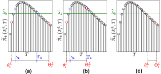
Figure 4: Graph of unimodal function $\widetilde{\mathcal{R}}_{k}\left(\mathcal{X}_{i}^{L},T\right)$ depicting an example when (a) $\gamma_{k}$ and $\Gamma_{k}$ exist and $\Gamma_{k}<\Theta_{i}^{L}$. (b) $\gamma_{k}$ and $\Gamma_{k}$ exist and $\Gamma_{k}=\Theta_{i}^{L}$. (c) $\gamma_{k}$ and $\Gamma_{k}$ do not exist.

To find all the sets $\widetilde{\mathcal{S}}\left(T\right)$ as $T$ varies in the interval $\left[\theta_{i}^{L},\Theta_{i}^{L}\right]$, we simply apply steps (A1) to (A4) to list $Q$. This is implemented in lines 16-20. Let $Q_{j}$ be the $j^{th}$ element of the sorted list $E$. If $Q_{j}.T<Q_{j+1}.T$, then $\mathcal{X}_{j}$ is one of the sets in $\mathcal{F}$. We have, $\widetilde{\mathcal{S}}\left(T\right)=\mathcal{X}_{j}\,;\,T\in\left[\theta_{j},\Theta_{j}\right]$ where $\theta_{j}=Q_{j}.T$ and $\Theta_{j}=Q_{j+1}.T-1$ . Therefore, the objective function in the interval $\left[\theta_{j},\Theta_{j}\right]$ is $\widetilde{U}\left(\mathcal{X}_{j},T\right)$ which is maximum for $T=\texttt{$\theta_{j}$}$ or $T=\Theta_{j}$ (Property 3). We can find the optimal lease duration in the interval $\left[\theta_{i}^{L},\Theta_{i}^{L}\right]$ by iterating over all $\mathcal{X}_{j}$ such that $Q_{j}.T<Q_{j+1}.T$. Finally, we can find the optimal lease duration $\widetilde{T}^{*}$ by repeating the same procedure for all such intervals $\left[\theta_{i}^{L},\Theta_{i}^{L}\right]$ that satisfies $Q_{i}^{L}.T<Q_{i+1}^{L}.T$. These steps are implemented in lines 21-25.

We end this section by discussing the time complexity of Algorithm 1 and comparing it with a bruteforce approach to solve $OP1$. Lines 12 and 22 are the most computationally demanding steps of Algorithm 1 as it involves numerical integration to evaluate the revenue function $\widetilde{\mathcal{R}}_{k}\left(\mathcal{S},T\right)$. All other computations is absorbed (up to a constant factor) by the time taken for evaluating the revenue function. Let $\widehat{\Lambda}^{L}=\underset{1\leq k\leq N}{\max}\widehat{\Lambda}_{k}$, the maximum lease duration above which none of the operators can afford a channel.

Proposition 4.

Time complexity of Algorithm 1 is $\mathcal{O}\left(N^{2}\log_{2}\left(\widehat{\Lambda}^{L}\right)+N^{3}\right)$.

Proof:

Please refer to Appendix F for the proof. ∎

A bruteforce approach to solve $OP1$ involves iterating from $T=1$ to $\widehat{\Lambda}^{L}$ to find the $T$ which maximizes $\widetilde{U}\left(T\right)$. This is because for $T>\widehat{\Lambda}^{L}$, $\widetilde{\mathcal{S}}\left(T\right)=\emptyset$ and hence $\widetilde{U}\left(T\right)=0$. To evaluate $\widetilde{U}\left(T\right)$, we need $\mathcal{O}\left(N\right)$ computations of $\widetilde{\mathcal{R}}_{k}\left(\mathcal{S},T\right)$ to find $\widetilde{\mathcal{S}}\left(T\right)$ (refer to (17)) and finally $\widetilde{U}\left(T\right)$ (refer to (13)). Therefore, time complexity of the bruteforce approach is $\mathcal{O}\left(N\widehat{\Lambda}^{L}\right)$. In practice, $\widehat{\Lambda}^{L}$ is much larger compared to $N$. Hence, time complexity of bruteforce approach, $\mathcal{O}\left(N\widehat{\Lambda}^{L}\right)$, is much larger compared to time complexity of Algorithm 1, $\mathcal{O}\left(N^{2}\log_{2}\left(\widehat{\Lambda}^{L}\right)+N^{3}\right)$.

IV Numerical Results

In Sections IV-A to IV-B, we use the optimization algorithms from Section III to numerically explore the effect of true market parameters $\xi_{k}$ on $\widetilde{T}^{*}$, $U^{*}=U\left(\mathcal{S}\left(\widetilde{T}^{*}\right),\widetilde{T}^{*}\right)$ and $s^{*}=\left|\mathcal{S}\left(\widetilde{T}^{*}\right)\right|$ for complete information games. Recall that $\widetilde{T}^{*}$ is the optimal lease duration corresponding to the perceived objective function, $U^{*}$ is the value of the objective function (true) corresponding to $\widetilde{T}^{*}$ and $s^{*}$ is the number of interested operators corresponding to $\widetilde{T}^{*}$ (refer to (21)). For complete information games, the perceived objective function, $\widetilde{U}\left(T\right)$, is equal to the objective function (true), $U\left(T\right)$. Hence, $\widetilde{T}^{*}=T^{*}$ here $T^{*}$ is the true optimal lease duration corresponding to $U\left(T\right)$. In Section IV-D, we discuss how incomplete information games leads to sub-optimal solutions.

One of the market parameters in $\xi_{k}$ is the autocorrelation coefficient $a_{k}$. Instead of $a_{k}$, we use time constant $\tau_{k}$ where $a_{k}=\exp\left(-\frac{1}{\tau_{k}}\right)$. A higher time constant implies higher autocorrelation. Throughout this section, number of operators $N=10$ and number of channels $M=2$.

IV-A Optimal Trends

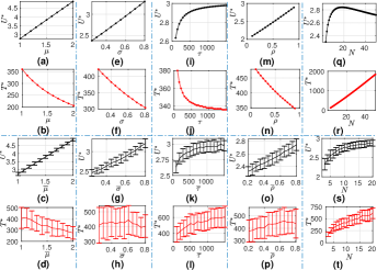
Figure 5: Plots showing $T^{*}$ and $U^{*}$ as a function of mean (a, b, c, and d), standard deviation (e, f, g, and h), time constant (i, j, k, and l), MER (m, n, o, and p), and number of operators (q, r, s, and t). The top two and the bottom two rows correspond to homogeneous and heterogeneous markets respectively. For every mean of the market parameters (x-axis) in a heterogeneous market, we averaged $T^{*}$ and $U^{*}$ over $100$ instances of market parameters.

The trends of $T^{*}$ and $U^{*}$ as a function of number of operators $N$ and parameters $\mu_{k}$, $\sigma_{k}$, $\tau_{k}$, and $\rho_{k}$ are discussed in this subsection. Throughout this subsection, $\Lambda_{k}=\infty\,;\,\forall k$. We consider both homogeneous and heterogeneous market. The default parameters for homogeneous market are $\mu=1$, $\sigma=0.5$, $\tau=100$, $\rho=0.8$ and $\lambda=100$. We vary one parameter at a time while holding the other parameters at their default values. We solve for $T^{*}$ and $U^{*}$ as we vary the parameters and plot the result in Figure 5.

For heterogeneous markets, we randomly choose the values for the market parameters from an uniform distribution. The default uniform distributions are $\mu_{k}\sim\mathcal{U}\left(0.8,1.2\right)$, $\sigma_{k}\sim\mathcal{U}\left(0.4,0.6\right)$, $\tau_{k}\sim\mathcal{U}\left(50,150\right)$, $\rho_{k}\sim\mathcal{U}\left(0.7,0.9\right)$, and $\lambda_{k}\sim\mathcal{U}\left(50,150\right)\,;\,\forall k$. Each of these distributions are associated with a mean and a range, e.g. the mean of $\mu_{k}$ is $\overline{\mu}=\frac{0.8+1.2}{2}=1$ and the range is $\left(1.2-0.8\right)=0.4$. The range of these distributions remains the same throughout this section; only the mean is varied. One of these distributions is varied at a time while holding the other distributions at their default value. For every distribution, we generate $100$ instances of market parameters sampled from the five distributions. We solve for $T^{*}$ and $U^{*}$ for each of the $100$ instances and plot the result as errorbar graphs in Figure 5. The errobar graphs show the sample mean and standard deviation of $T^{*}$ and $U^{*}$.

We will now explain the effect of various parameters on $T^{*}$ and $U^{*}$. These explanations will rely on Properties 1 - 4. Also, recall that special cases of Properties 3 and 4 holds for homogeneous market, i.e. objective function is monotonic decreasing in $T$ (Property 3) and monotonic increasing in $s$ (Property 4) for a homogeneous market.

Effect of mean: In a homogeneous market, as $\mu$ increases, an operator’s revenue per time slot increases. Therefore, it will take less time to generate the MER $\lambda$. Hence, $T^{*}$ decreases as shown in Figure 5.b. With decrease in $T^{*}$, $U^{*}$ increases according to Property 3. This is shown in Figure 5.a. Similar trends hold for heterogeneous market. As the mean of $\mu_{k}$, $\overline{\mu}$, increases, the sample mean of $U^{*}$ increases while the sample mean of $T^{*}$ decreases. This is shown in Figures 5.c. and 5.d.

Effect of standard deviation: In a homogeneous market, $T^{*}$ decreases with increase in $\sigma$ as shown in Figure 5.f. This can be explained as follows. As $\sigma$ increases, an operator’s revenue fluctuates more around the mean. These fluctuations can lead to a revenue which is either greater or lower than the mean. If an operator is allocated a channel, there is a higher probability that the revenue is greater than the mean. This is due to the allocation policy which, in general, ensures that the operator who is allocated a channel has a high revenue. This suggests that the revenue function increases with $\sigma$. Since the revenue function increases, an operator takes less time to generate its MER. Hence, $T^{*}$ decreases with increase in $\sigma$. As $T^{*}$ decreases, $U^{*}$ increases due to Property 3. This is shown in Figure 5.e. For a heterogeneous market, the sample mean of $U^{*}$ increases with increase in mean of $\sigma_{k}$, $\overline{\sigma}$. This is shown in Figure 5.g and its is similar to homogeneous market. However, unlike a homogeneous market, the sample mean of $T^{*}$ remains almost the same with increase in $\overline{\sigma}$ as shown in Figure 5.h. This happens due to a cyclic effect which can be explained as follows. Similar to homogeneous market, with increase in $\overline{\sigma}$, the revenue function increases. But as the revenue function increases, more operators are interested in entering the market which in turn decreases the revenue function (Property 2). These two competing factors negates the impact of $\overline{\sigma}$ on the revenue function and hence on $T^{*}$.

Effect of time constant: Consider the homogeneous market first. Autocorrelation defines the self-similarity of a random process. As autocorrelation increases, an operator with higher revenue at current time slot will have higher revenue at a later time slot. Therefore, with increase in time constant $\tau$ (and hence autocorrelation), the revenue function increases. As the revenue function increases, an operator takes less time to generate its MER. Hence, $T^{*}$ decreases with increase in $\tau$. As $T^{*}$ decreases, $U^{*}$ increases due to Property 3. This is shown in Figure 5.i and 5.j. For a heterogeneous market, the sample mean of $U^{*}$ increases with increase in mean of $\tau_{k}$, $\overline{\tau}$. This trend is shown in Figure 5.k and its is similar to a homogeneous market. However, unlike a homogeneous market, the sample mean of $T^{*}$ increases with increase in $\overline{\tau}$ as shown in Figure 5.l. This is due to the same cyclic effect mentioned while explaining the effect of standard deviation. But in this case, the effect of the increase in number of interested operator is more dominant. As a result, the revenue function decreases with increase in $\overline{\tau}$. Since the revenue function decreases, the sample mean of $T^{*}$ increases because an operator takes more time to generate its MER.

Effect of bid correlation coefficient: Consider the homogeneous market first. As bid correlation coefficient increases, an operator with a high bid is more likely to generate a higher revenue. Since channels are allocated to operators with high bids, we can equivalently say that if an operator is allocated a channel, then its revenue increases with increase in bid correlation coefficient. Therefore, it will take less time to generate the MER $\lambda$. Hence, $T^{*}$ decreases with increase in $\rho$. With decrease in $T^{*}$, $U^{*}$ increases according to Property 3. This is shown in Figure 5.m and Figure 5.n. For a heterogeneous market, the sample mean of $U^{*}$ increases with increase in mean of $\rho_{k}$, $\overline{\rho}$. This is shown in Figure 5.o and its is similar to a homogeneous market. However, unlike a homogeneous market, the sample mean of $T^{*}$ increases with increase in $\overline{\rho}$ as shown in Figure 5.p. This is due to the same cyclic effect mentioned while explaining the effect of time constant.

Effect of number of operators: Consider the homogeneous market first. As the number of operators increases, the probability that a given operator is allocated a channel decreases. To compensate for this decrease in probability, an operator has to generate more revenue when it is allocated a channel in order to satisfy its MER. Hence, $T^{*}$ increases as shown in Figure 5.r. Now we will explain the effect of $N$ on $U^{*}$. As $N$ increases, $U^{*}$ increases according to Property 4. However, with increase in $N$, $T^{*}$ increases which leads to decrease in $U^{*}$ according to Property 3. Because of these two competing factors, $U^{*}$ first increases and then decreases with increase in $N$ as shown in Figure 5.q. Recall that in our model, the number of interested operators is a measure of market competition. Then this numerical study shows that too much competition may not necessarily improve spectrum utilization.

For heterogeneous market, we sampled $\mu_{k}$, $\sigma_{k}$, $\tau_{k}$, $\rho_{k}$ and $\lambda_{k}$ from their default uniform distributions. As $N$ increases, the sample mean of $T^{*}$ and $U^{*}$ increases. This is shown in Figure 5.s and 5.t. These trends are similar to homogeneous market. Similar to homogeneous market, we expect the sample mean of $U^{*}$ to start decreasing if $N$ is above a threshold. But, we could not verify the same. This is because as $N$ increases, computing the revenue function for a heterogeneous market becomes computationally expensive which in turn makes Algorithm 1 computationally expensive. This problem does not exists for homogeneous market because the expression for revenue function is simpler for homogeneous market. Please refer to the proof of Propositions 5 and equation 60 in the appendix to appreciate the relative complexity of the revenue function for a heterogeneous and a homogeneous market.

IV-B Comparison with an intuitive algorithm

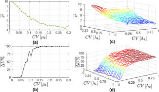
Figure 6: Plots comparing the performance of Algorithm 1 and SUBOP as the market becomes more heterogeneous in Mean $\mu_{k}$ (a, b), MER $\lambda_{k}$ and maximum affordable lease duration $\Lambda_{k}$ (c, d). In (a, b), for each coefficient of variation $CV\left[\mu_{k}\right]$, $\overline{s^{*}}$ and $\overline{\Delta U_{\%}}$ have been averaged over $100$ instance of $\mu_{k}$. In (c, d), for each pair of coefficient of variations $\left(CV\left[\lambda_{k}\right],CV\left[\Lambda_{k}\right]\right)$, $\overline{s^{*}}$ and $\overline{\Delta U_{\%}}$ have been averaged over $100$ instance of $\lambda_{k}$ and $\Lambda_{k}$.

In this section, we compare the performance of Algorithm 1 with an intuitive, but sub-optimal, algorithm SUBOP which maximizes the objective function by setting a lease duration that satisfies all the $N$ operators in terms of affordability $\Lambda_{k}$ and MER $\lambda_{k}$. Through this comparison we exemplify that as the market becomes more heterogeneous, it is not optimal to satisfy all the operators even if it is possible.

We start by describing SUBOP. Define $\mathcal{S}_{N}=\left\{1,2,\ldots,N\right\}$. Since SUBOP has to satisfy all the $N$ operators, the $k^{th}$ operator is satisfied if the lease duration satisfies $T\leq\Lambda_{k}$ and $\mathcal{R}_{k}\left(\mathcal{S}_{N},T\right)\geq\lambda_{k}$. The solution to $\mathcal{R}_{k}\left(\mathcal{S}_{N},T\right)\geq\lambda_{k}$ is a range $\left[\gamma_{k},\Gamma_{k}\right]$ (refer to line 1 of Algorithm 1). But $T\leq\Lambda_{k}$ and hence the range has to be modified as $\left[\widetilde{\gamma}_{k},\widetilde{\Gamma}_{k}\right]$ where $\widetilde{\gamma}_{k}=\gamma_{k}$ and $\widetilde{\Gamma}_{k}=\min\left(\Gamma_{k},\Lambda_{k}\right)$. The $k^{th}$ operator is interested in entering the market iff $T\in\left[\widetilde{\gamma}_{k},\widetilde{\Gamma}_{k}\right]$. The range of lease duration that satisfies all the $N$ operators is $\left[\widetilde{\theta},\widetilde{\Theta}\right]$ where $\widetilde{\theta}=\underset{k}{\max}\>\widetilde{\gamma}_{k}$ and $\widetilde{\Theta}=\underset{k}{\min}\>\widetilde{\Gamma}_{k}$. If $\widetilde{\Theta}<\widetilde{\theta}$, then there is no lease duration that satisfies all the operators and hence the value of the objective function is $U_{S}^{*}=0$ where the subscript $S$ implies sub-optimal. If $\widetilde{\Theta}\geq\widetilde{\theta}$, then either $T=\widetilde{\theta}$ or $T=\widetilde{\Theta}$ maximizes the objective function (Property 3) subjected to $\mathcal{S}=\mathcal{S}_{N}$. Accordingly, the value of the objective function is $U_{S}^{*}=\max\left(U\left(\mathcal{S}_{N},\widetilde{\theta}\right),U\left(\mathcal{S}_{N},\widetilde{\Theta}\right)\right)$.

We first compare the performance of Algorithm 1 with SUBOP as the market becomes more heterogeneous in mean $\mu_{k}$. To compare the algorithms, lets define $\Delta U_{\%}$=$\frac{U^{*}-U_{S}^{*}}{U_{S}^{*}}\times$100, the percentage increase in $U^{*}$ compared to $U_{s}^{*}$. The setup is homogeneous in all market parameters but $\mu_{k}$. We have $\sigma_{k}=0.5$, $\tau_{k}=100$, $\lambda_{k}=100$, and $\Lambda_{k}=\infty\,;\,\forall k$. The mean $\mu_{k}$ is sampled from a truncated gaussian distribution with mean $1$, coefficient of variation $CV\left[\mu_{k}\right]$ and the truncation bounds are $0.5$ and $1.5$. As $CV\left[\mu_{k}\right]$ increases, the gaussian distribution spreads out more and hence there is a wider range of $\mu_{k}$ making the market more heterogeneous. As shown in Figure 6.a, expected optimal number of interested operators $\overline{s^{*}}$ decreases with increase in $CV\left[\mu_{k}\right]$. This is because as the market becomes more heterogeneous in $\mu_{k}$, the revenue function becomes unimodal in nature (Property 1). This suggests that there may not be a lease duration that satisfies MER of all the operators. Even if it is possible to satisfy lease duration of all the operators, such lease durations may too large which may significantly decrease the objective function according to Property 3 (assuming bid correlation coefficients of the operators are high). It is also possible that some of the operators have low bid correlation coefficient. If they enter the market, objective function function can decrease (Property 4). Therefore, it may not be optimal to satisfy those operators whose bid correlation coefficient is low. But since SUBOP tries to satisfy all the operators, its performance compared to Algorithm 1 decreases as the market becomes more heterogeneous in $\mu_{k}$. This is shown in Figure 6.b. where $\overline{\Delta U_{\%}}$ increases with $CV\left[\mu_{k}\right]$.

Similarly, we compare the performance of Algorithm 1 with SUBOP as the market becomes more heterogeneous in $\lambda_{k}$ and $\Lambda_{k}$. The setup is homogeneous in all market parameters but $\lambda_{k}$ and $\Lambda_{k}$. We have $\mu_{k}=1$, $\sigma_{k}=0.5$ and $\tau_{k}=100\,;\,\forall k$. $\lambda_{k}$ is sampled from a truncated gaussian distribution with mean $500$, coefficient of variation $CV\left[\lambda_{k}\right]$ and the truncation bounds are $100$ and $900$. $\Lambda_{k}$ is sampled from a truncated gaussian distribution with mean $5000$, coefficient of variation $CV\left[\Lambda_{k}\right]$ and the truncation bounds are $900$ and $9100$. As $CV\left[\lambda_{k}\right]$ and $CV\left[\Lambda_{k}\right]$ increases, there is a wider of $\lambda_{k}$ and $\Lambda_{k}$. As shown in Figure 6.c, expected optimal number of interested operators $\overline{s^{*}}$ decreases with increase in $CV\left[\lambda_{k}\right]$ and $CV\left[\Lambda_{k}\right]$. This is because as the market becomes more heterogeneous in $\lambda_{k}$ and $\Lambda_{k}$, it is possible that a lease duration that satisfies MER of one operator is not affordable by another operator. Hence, there may not exist a lease duration that satisfies all the operator. Even if it is possible to satisfy lease duration of all the operators, such lease durations may be too large because few of the operators have high MER. Setting such a large lease duration may not be optimal according to Property 3. But since SUBOP tries to satisfy all the operators, its performance compared to Algorithm 1 decreases as the market becomes more heterogeneous in $\lambda_{k}$ and $\Lambda_{k}$. This is shown in Figure 6.d.

IV-C Discontinuity in Optimal Trends

This numerical result deals with complete information games. We demonstrate certain interesting discontinuities in optimal trends as MER of operators changes in a heterogeneous market. Since we are considering complete information games, we have $\widehat{\xi}_{k}=\xi_{k}\,;\,\forall k$, and hence $\mathcal{S}_{k}^{L}\left(T\right)$ is same for all $k$’s (refer to (16)). So we have, $\mathcal{S}_{k}^{L}\left(T\right)=\mathcal{S}^{L}\left(T\right)\,;\,\forall k$. Let $s^{L*}=\left|\mathcal{S}^{L}\left(T^{*}\right)\right|$ denote the largest number of interested operators corresponding to optimal lease duration. The numerical setup is as follows. The market is homogeneous in all parameters but $\lambda_{k}$. We have $\mu_{k}=\mu=1\,;\,\forall k$, $\sigma_{k}=\sigma=0.5\,;\,\forall k$, $\tau_{k}=\tau=100\,;\,\forall k$ and $\Lambda_{k}=\infty\,;\,\forall k$. MER of the first $8$ operators are $100$ while the $9^{th}$ and the $10^{th}$ operator has MER $\overline{\lambda}\geq 100$. As our setup is homogeneous in $\mu_{k}$, $\sigma_{k}$ and $\tau_{k}$, the revenue function of all the operators is $\mathcal{R}\left(s,T\right)$ and the objective function is $U\left(s,T\right)$ (refer to Section II-C). Recall that $U\left(s,T\right)$ is monotonic decreasing in $T$ (special case of Property 3) and monotonic increasing in $s$ (special case of Property 4) while $\mathcal{R}\left(s,T\right)$ is monotonic increasing in $T$ (special case of Property 1). Consider if the market consists of only the first $8$ operators. This market is completely homogeneous and the optimal lease duration is the solution to $\mathcal{R}\left(8,T\right)=100$ (refer to Section III-A) which is equal to $306$. Now consider the market with all the $10$ operators. The optimal lease duration of this market must be at least $306$ because the MER of the first $8$ operators must be satisfied for optimality. We explore how $U^{*}$, $T^{*}$, $s^{*}$ and $s^{L*}$ vary with $\overline{\lambda}$.

As $\overline{\lambda}$ varies, there are three discontinuities in $U^{*}$, $T^{*}$, $s^{*}$ and $s^{L*}$ as shown in Figure 7. Therefore, we divide our explanation into three regions. As mentioned in the previous paragraph, $T^{*}\geq 306$. In region G1, $\overline{\lambda}\leq\mu T^{*}\leq 306$, implying that the $9^{th}$ and the $10^{th}$ operator may join the market along with the other $8$ operators. Hence, $s^{L*}=\left|\mathcal{S}^{L}\left(T^{*}\right)\right|=10$ (refer to (16)). Therefore, the minimum value of the revenue function is $\mathcal{R}\left(10,T\right)$ which decides whether an operator is interested in entering the market (refer to Section II-D). There are two possible candidates for optimal lease duration. First, the lease duration is $T_{1}$ that satisfies $\mathcal{R}\left(10,T_{1}\right)=100$. In this case, only the first $8$ operators are interested in entering the market and hence the value of the objective function is $U\left(8,T_{1}\right)$. Second, the lease duration is $T_{2}$ that satisfies $\mathcal{R}\left(10,T_{2}\right)=\overline{\lambda}$. Since $\overline{\lambda}\geq 100$, all the $10$ operators are interested in entering the market and hence the value of the objective function is $U\left(10,T_{2}\right)$. Definitely, $T_{2}\geq T_{1}$ because $\overline{\lambda}\geq 100$ and the $\mathcal{R}\left(s,T\right)$ is monotonic increasing in $T$. In region G1, $T_{2}$ is not much larger compared to $T_{1}$ because $\overline{\lambda}$ is very close to $100$. Hence, according to Property 4, $U\left(10,T_{2}\right)>U\left(8,T_{1}\right)$. Therefore, $T^{*}=T_{2}$, $s^{*}=10$ and $U^{*}=U\left(10,T_{2}\right)$. This is shown in Figure 7.a, 7.b and 7.c. As $\overline{\lambda}$ increases, $T^{*}=T_{2}$ increases and hence $U^{*}=U\left(10,T_{2}\right)$ decreases (Property 3).

In region G2, $\overline{\lambda}$ is much more than $100$ and hence $T_{2}$ is much larger compared to $T_{1}$. Hence, according to Property 3, $U\left(10,T_{2}\right)<U\left(8,T_{1}\right)$. Therefore, $T^{*}=T_{1}$, $s^{*}=8$ and $U^{*}=U\left(8,T_{1}\right)$. This is shown in Figure 7.a, 7.b and 7.c. As $T_{1}$ is a constant, $T^{*}$ and $U^{*}$ are constants in region G2. In region G3, $\overline{\lambda}>306$ as shown in Figure 7.a. Since it was not optimal to satisfy MER of the $9^{th}$ and the $10^{th}$ operator in region G2, it is not optimal to satisfy their MER in region G3. This is because $\overline{\lambda}$ in region G3 is greater compared to region G2. But we must satisfy the MER of first $8$ operators. Say that the lease duration is $306$. It is the least lease duration that satisfies MER of the first $8$ operators. Also, it does not satisfy MER of the $9^{th}$ and the $10^{th}$ operator becasuse $\overline{\lambda}>306$. Infact, if lease duration is $306$, the dominant strategy of the $9^{th}$ and the $10^{th}$ operator is not to enter the market and hence $s^{L*}=8$ as shown in Figure 7.d. So we conlude that $T^{*}=306$ in region G3 and the corresponding $U^{*}=U\left(8,306\right)=2.61$. This is shown in Figure 7.a and 7.b.

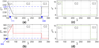
Figure 7: A figure demonstrating the discontinuous nature of $U^{*}$, $T^{*}$, $s^{*}$ and $s^{L*}$ as a function of MER $\overline{\lambda}$.

We conclude this section with two critical observations. If the market consisted of only the first $8$ operators, then $U^{*}$=2.61. With the $9^{th}$ and the $10^{th}$ operator in the market, $U^{*}$ is less than $2.61$ if $\overline{\lambda}$ lies in the interval $\left(111,308\right)$. This is shown in Figure 7.a. Based on this observation, we can conclude the following. First, too much competition may not necessarily lead to better spectrum utilization. In region G1, even though all the $10$ operators are interested in entering the market, $U^{*}$ is less than $2.61$ if $\overline{\lambda}>111$. Second, as a thumb rule, the spectrum utilization is higher if the MER of the operators are low and hence leading to a lower lease duration or if the MER is high enough that it does not affect the decision of the other operators to enter the market. To appreciate the last point, note that in region G2, the first $8$ operators enter the market only if their MER is satisfied even if all $10$ operator enters the market. So, even though the $9^{th}$ and the $10^{th}$ operators did not enter the market, these two operators affected the decision of the first $8$ operators.

IV-D Effect of Incomplete Information

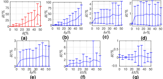
Figure 8: Plots of $\delta U\%$, the relative change in the optimal value of the objective function due to incomplete information, when there is a error in (a) all the parameters in $\widehat{\xi}_{k}$, (b) $\widehat{\mu}_{k}$, (c) $\widehat{\sigma}_{k}$, (d) $\widehat{\tau}_{k}$, (e) $\widehat{\rho}_{k}$, (f) $\widehat{\lambda}_{k}$, and (g) $\widehat{\Lambda}_{k}$.

Our final numerical study analyzes how the deviation of the estimated market parameters, $\widehat{\xi}_{k}$, from the true market parameters, $\xi_{k}$, leads to sub-optimal spectrum utilization. Recall that $\widetilde{T}^{*}$ is the optimal lease duration corresponding to estimated market parameters, $\widehat{\xi}_{k}$. $\widetilde{T}^{*}$ is one of the outputs of Algorithm 1 of the main paper. Let $T^{*}$ be the optimal lease duration corresponding to true market parameters, $\xi_{k}$. In other words, $\widetilde{T}^{*}=T^{*}$ when $\widehat{\xi}_{k}=\xi_{k}$. The value of the objective function (true) corresponding to $\widetilde{T}^{*}$ and $T^{*}$ are $U\left(\mathcal{S}\left(\widetilde{T}^{*}\right),\widetilde{T}^{*}\right)$ and $U\left(\mathcal{S}\left(T^{*}\right),T^{*}\right)$ respectively (refer to (21) of the main paper). Let,

$$\delta U\%=\frac{U\left(\mathcal{S}\left(T^{*}\right),T^{*}\right)-U\left(\mathcal{S}\left(\widetilde{T}^{*}\right),\widetilde{T}^{*}\right)}{U\left(\mathcal{S}\left(T^{*}\right),T^{*}\right)}\cdot 100$$

$\delta U\%$ is the relative change in the optimal value of the objective function (spectrum utilization) due to incomplete information. We randomly choose true market parameters from uniform distributions: $\mu_{k}\sim\mathcal{U}\left(0.8,1.2\right)$, $\sigma_{k}\sim\mathcal{U}\left(0.4,0.6\right)$, $\tau_{k}\sim\mathcal{U}\left(150,250\right)$, $\rho_{k}\sim\mathcal{U}\left(0.5,0.7\right)$, $\lambda_{k}\sim\mathcal{U}\left(50,150\right)$, and $\Lambda_{k}\sim\mathcal{U}\left(500,2000\right)\,;\,\forall k$. Consider the true parameter $\mu_{k}$. The estimated parameter $\widehat{\mu}_{k}$ is choosen uniformly at random in the interval $\left[\mu_{k}-\frac{\delta\mu\%}{100}\cdot\mu_{k},\mu_{k}+\frac{\delta\mu\%}{100}\cdot\mu_{k}\right]$ where $\delta\mu\%$ is the error window associated with $\mu_{k}$. Similarly, we have error windows $\delta\sigma\%$, $\delta\tau\%$, $\delta\rho\%$, $\delta\lambda\%$ and $\delta\Lambda\%$ associated with $\sigma_{k}$, $\tau_{k}$, $\rho_{k}$, $\lambda_{k}$ and $\Lambda_{k}$ respectively. In Figure 8, we plot errorbar graphs to study how $\delta U\%$ vary with error window. In Figure 8.a, all the six error windows are varied while in the remaining six plots, one of the error windows is varied while the remaining five error windows are set to zero. For each value of error window, we sample over $100$ random instances of true and estimated market parameters to generate the errorbar graphs.

As expected, the sample mean of $\delta U\%$ increases with error window. Comparing Figure 8.a with the remaining six graphs, we can conclude that most of the reduction in spectrum utilization happens due to error in $\mu_{k}$. Finally, we point to a non-intuitive result which can be observed by zooming into Figure 8. There are some cases where $\delta U\%$ is less than zero. In other words, it is possible that in an incomplete information scenario, spectrum utilization is more than complete information scenario. This can happen when an operator makes an erroneous decision of joining the market (not joining the market) due to error in $\widehat{\xi}_{k}$. This can improve spectrum utilization if the true bid correlation coefficient is high (low).

V Conclusion

The duration of a spectrum lease is a critical parameter that influences the efficiency of spectrum utilization. The main contribution of this paper is a mathematical model that is used to find the lease duration which maximizes spectrum utilization. This model captures the effects of lease duration on spectrum utilization for a market where an operators’ revenue is a measure of its spectrum utilization. Based on the system model, we formulate a Stackelberg game with lease duration as one of the decision variables. We also design algorithms to find the Stackelberg equilibrium and hence find the optimal lease duration. Using these algorithms, we find several numerical trends that show how lease duration should change with respect to various market parameters in order to maximize spectrum utilization.

There are several possible avenues for extending this work, including: (a) Generalization of our system model to capture the transaction costs associated with re-allocation of channels. (b) Including variance in our system model to capture risk aversion of the operators. (c) Second price auctions to capture the variable market-dependent price of a spectrum lease.

Appendix A Proof of Proposition 1

We want to find the probability density function (pdf ) of the random variable $Y_{k}\left(c,T\right)=\stackrel{{\scriptstyle[}}{{t}}=\left(c-1\right)T+1]{cT}{\sum}x_{k}\left(t\right)$. Since $x_{k}\left(t\right)$ is a stationary process, the pdf of $Y_{k}\left(c,T\right)$ is same for all epochs. Therefore, we can simply derive the pdf of $Y_{k}\left(1,T\right)=\stackrel{{\scriptstyle[}}{{t}}=1]{T}{\sum}x_{k}\left(t\right)$. Now, $Y_{k}\left(1,T\right)$ is gaussian because $x_{k}\left(t\right)$ is gaussian and sum of gaussian random variable is always gaussian. Since $Y_{k}\left(1,T\right)$ is gaussian, its pdf is completely characterized by its mean $\widetilde{\mu}_{k}\left(T\right)$ and standard deviation $\widetilde{\sigma}_{k}\left(T\right)$. Based on this discussion we can conclude that

$$Y_{k}\left(c,T\right)\sim\mathcal{N}\left(\widetilde{\mu}_{k}\left(T\right),\widetilde{\sigma}_{k}^{2}\left(T\right)\right)\,;\,\forall c$$ (22)

Now all we have to do is to find expressions for $\widetilde{\mu}_{k}\left(T\right)$ and $\widetilde{\sigma}_{k}\left(T\right)$. We have,

$$\widetilde{\mu}_{k}\left(T\right)=E\left[\stackrel{{\scriptstyle[}}{{t}}=1]{T}{\sum}x_{k}\left(t\right)\right]=\stackrel{{\scriptstyle[}}{{t}}=1]{T}{\sum}E\left[x_{k}\left(t\right)\right]=\mu_{k}T$$ (23)

For a first order AR process as governed by (1), $x_{k}\left(t\right)$ can be expressed as

$$x_{k}\left(t\right)=a_{k}^{t}x_{k}\left(0\right)+\stackrel{{\scriptstyle[}}{{v}}=0]{t-1}{\sum}a_{k}^{t-1-v}\varepsilon_{k}\left(v\right)$$ (24)

Equation 24 can be easily proved using mathematical induction. Also,

$$\stackrel{{\scriptstyle[}}{{t}}=1]{T}{\sum}x_{k}\left(t\right) = \stackrel{{\scriptstyle[}}{{t}}=1]{T}{\sum}\left(a_{k}^{t}x_{k}\left(0\right)+\stackrel{{\scriptstyle[}}{{v}}=0]{t-1}{\sum}a_{k}^{t-1-v}\varepsilon_{k}\left(v\right)\right)$$

$$= x_{k}\left(0\right)\stackrel{{\scriptstyle[}}{{t}}=1]{T}{\sum}a_{k}^{t}+\stackrel{{\scriptstyle[}}{{t}}=1]{T}{\sum}\stackrel{{\scriptstyle[}}{{v}}=0]{t-1}{\sum}a_{k}^{t-1-v}\varepsilon_{k}\left(v\right)$$

$$= x_{k}\left(0\right)\stackrel{{\scriptstyle[}}{{t}}=1]{T}{\sum}a_{k}^{t}+\stackrel{{\scriptstyle[}}{{v}}=0]{T-1}{\sum}\stackrel{{\scriptstyle[}}{{t}}=v+1]{T}{\sum}a_{k}^{t-1-v}\varepsilon_{k}\left(v\right)$$ (26)

$$= x_{k}\left(0\right)\frac{a_{k}-a_{k}^{T+1}}{1-a_{k}}+\stackrel{{\scriptstyle[}}{{v}}=0]{T-1}{\sum}\frac{1-a_{k}^{T-v}}{1-a_{k}}\varepsilon_{k}\left(v\right)\;\;\;\;\;\;$$ (27)

Equation A is obtained using (24). Equation 26 is obtained by changing the order of summation. Now, $\widetilde{\sigma}_{k}\left(T\right)=\sqrt{\text{Var}\left[\stackrel{{\scriptstyle[}}{{t}}=1]{T}{\sum}x_{k}\left(t\right)\right]}$ where,

$$\text{Var}\left[\stackrel{{\scriptstyle[}}{{t}}=1]{T}{\sum}x_{k}\left(t\right)\right]$$ (29)

$$= \text{Var}\left[x_{k}\left(0\right)\frac{a_{k}-a_{k}^{T+1}}{1-a_{k}}+\stackrel{{\scriptstyle[}}{{v}}=0]{T-1}{\sum}\frac{1-a_{k}^{T-v}}{1-a_{k}}\varepsilon_{i}\left(v\right)\right]$$

$$= \left(\frac{a_{k}-a_{k}^{T+1}}{1-a_{k}}\right)^{2}\text{Var}\left[x_{k}\left(0\right)\right]$$

$$\qquad+\stackrel{{\scriptstyle[}}{{v}}=0]{T-1}{\sum}\left(\frac{1-a_{k}^{T-v}}{1-a_{k}}\right)^{2}\text{Var}\left[\varepsilon_{k}\left(v\right)\right]$$

$$= \left(\frac{a_{k}-a_{k}^{T+1}}{1-a_{k}}\right)^{2}\sigma_{k}^{2}+\stackrel{{\scriptstyle[}}{{v}}=0]{T-1}{\sum}\left(\frac{1-a_{k}^{T-v}}{1-a_{k}}\right)^{2}\left(\sigma_{k}^{\varepsilon}\right)^{2}$$

$$= \frac{T-a_{k}\left(2-2a_{k}^{T}+a_{k}T\right)}{\left(1-a_{k}\right)^{2}}\cdot\frac{\left(\sigma_{k}^{\varepsilon}\right)^{2}}{1-a_{k}^{2}}$$

$$= \frac{T-a_{k}\left(2-2a_{k}^{T}+a_{k}T\right)}{\left(1-a_{k}\right)^{2}}\sigma_{k}^{2}$$ (31)

So we have,

$$\widetilde{\sigma}_{k}\left(T\right)=\frac{\sqrt{T-a_{k}\left(2-2a_{k}^{T}+a_{k}T\right)}}{\left(1-a_{k}\right)}\sigma_{k}$$ (32)

Equation 29 is obtained from (27). Equation A holds because $\varepsilon_{k}\left(v\right)$ are independent random variables. Equations A and 31 follows from the definition of $\sigma_{i}^{\varepsilon}$ and $\sigma_{i}$ as given by (2) and the paragraph before it. Finally, (23) and (32) are same as (3) and (4) respectively. This completes the proof.

Appendix B Revenue Function for Heterogeneous Market

In this section, we will derive an expression for the revenue function $\mathcal{R}_{k}\left(\mathcal{S},T\right)$ for a heterogeneous market. Let’s redefine few notations from the main paper for the sake of continuity. Recall the following from the main paper. $Y_{k}\left(c,T\right)$ is the net revenue of the $k^{th}$ operator in $c^{th}$ epoch if lease duration is $T$. $\widehat{Y}_{k}\left(c,T\right)$ is the bid of the $k^{th}$ operator in $c^{th}$ epoch if lease duration is $T$. For notational simplicity, lets denote $Y_{k}\left(c,T\right)$ by $Y_{k}$ and $\widehat{Y}_{k}\left(c,T\right)$ by $\widehat{Y}_{k}$. According to equation 5, the joint probability distribution of $\widehat{Y}_{k}$ and $Y_{k}$ is

$$\begin{bmatrix}Y_{k}\\ \widehat{Y}_{k}\end{bmatrix}\sim\mathcal{N}\left(\begin{bmatrix}\widetilde{\mu}_{k}\left(T\right)\\ \widetilde{\mu}_{k}\left(T\right)\end{bmatrix},\begin{bmatrix}\widetilde{\sigma}_{k}^{2}\left(T\right)&\rho_{k}\widetilde{\sigma}_{k}^{2}\left(T\right)\\ \rho_{k}\widetilde{\sigma}_{k}^{2}\left(T\right)&\widetilde{\sigma}_{k}^{2}\left(T\right)\end{bmatrix}\right)\,;\,\forall c$$ (33)

According to equation 6, the marginal distribution as $\widehat{Y}_{k}$ is

$$\widehat{Y}_{k}\sim\mathcal{N}\left(\widetilde{\mu}_{k}\left(T\right),\widetilde{\sigma}_{k}^{2}\left(T\right)\right)\,;\,\forall c$$ (34)

Proposition 5. Say that in every epoch, one channel is allocated to each of the $\widetilde{M}=\min\left(M,s\right)$ operators having the $\widetilde{M}$ highest sum of revenue in that epoch. Let $\mathcal{S}_{k}=\mathcal{S}-\left\{k\right\}$ and $\mathcal{C}\left(A,a\right)$ denote all the possible combinations of size $a-1$ from set $A$ . Let the function $f_{k}\left(Y,\widehat{Y},T\right)$ denote the probability density function (pdf) corresponding to the joint distribution of bid $\widehat{Y}$ and true revenue $Y$ of the $k^{th}$ operator as given by (33). Similarly, let the function $F_{k}\left(\widehat{Y},T\right)$ denote the cumulative distribution function (cdf) corresponding to the marginal distribution of bid $\widehat{Y}$ of the $k^{th}$ operator as given by (34). Then the revenue function of the $k^{th}$ operator is

$$\mathcal{R}_{k}\left(\mathcal{S},T\right)=\stackrel{{\scriptstyle[}}{{-}}\infty]{\infty}{\int}\>\stackrel{{\scriptstyle[}}{{-}}\infty]{\infty}{\int}Y\cdot\mathcal{G}_{k}\left(\widehat{Y},\mathcal{S},T\right)\cdot f_{k}\left(Y,\widehat{Y},T\right)\,dY\,d\widehat{Y}$$ (35)

where,

$$\mathcal{G}_{k}\left(\widehat{Y},\mathcal{S},T\right)=\stackrel{{\scriptstyle[}}{{m}}=1]{\widetilde{M}}{\sum}\>\underset{W\in\mathcal{C}\left(\mathcal{S}_{k},m\right)}{\sum}\mathcal{H}_{k}\left(\widehat{Y},T,W\right)$$ (36)

$$\mathcal{H}_{k}\left(\widehat{Y},T,W\right)=\underset{j\in W}{\prod}\left(1-F_{j}\left(\widehat{Y},T\right)\right)\underset{j\in\mathcal{S}_{k}-W}{\prod}F_{j}\left(\widehat{Y},T\right)$$ (37)

Proof. Consider the term $E\left[Y_{k}\left(1,T\right)|w_{1}^{m}=k\right]P\left[w_{1}^{m}=k\right]$ of (8). We have,

$$E\left[Y_{k}\left(1,T\right)|w_{1}^{m}=k\right]P\left[w_{1}^{m}=k\right]$$ (39)

$$= \underset{Y}{\sum}YP\left[Y_{k}=Y|w_{1}^{m}=k\right]P\left[w_{1}^{m}=k\right]$$

$$= \underset{\widehat{Y},Y}{\sum}YP\left[Y_{k}=Y,\widehat{Y}_{k}=\widehat{Y}|w_{1}^{m}=k\right]P\left[w_{1}^{m}=k\right]$$

$$= \underset{\widehat{Y},Y}{\sum}YP\left[{\textstyle w_{1}^{m}=k\,|\,Y_{k}=Y,\widehat{Y}_{k}=\widehat{Y}}\right]P\left[Y_{k}=Y,\right.$$

$$\qquad\qquad\qquad\qquad\qquad\qquad\qquad\qquad\left.\widehat{Y}_{k}=\widehat{Y}\right]$$

$$= \underset{\widehat{Y},Y}{\sum}YP\left[w_{1}^{m}=k|\widehat{Y}_{k}=\widehat{Y}\right]P\left[Y_{k}=Y,\widehat{Y}_{k}=\widehat{Y}\right]$$ (40)

Equation 39 is obtained by marginalizing over bid $\widehat{Y}_{k}$, (39) is obtained using Bayes’ Theorem and (40) is true because given $\widehat{Y}_{k}$, $w_{1}^{m}$ is independent of $Y_{k}$ (spectrum allocation depends on operators’ bid in an epoch and not on its net revenue in an epoch). $\widetilde{M}=\min\left(M\,,\,s\right)$ channels are allocated in every epoch. As mentioned in the main paper (first paragraph of section II-B), $w_{1}^{m}$ is the operator who has the $m^{th}$ highest value of $\widehat{Y}_{k}$ where $m$ is the channel index. Let $\bigcap$ denote the logical AND operator. Then the event $w_{1}^{m}=k$ is equivalent to

$$\underset{j\in W}{\bigcap}\,\widehat{Y}_{j}\geq\widehat{Y}_{k}\>,\>\underset{j\in\mathcal{S}_{k}-W}{\bigcap}\,\widehat{Y}_{j}\leq\widehat{Y}_{k}$$

for some $W\in\mathcal{C}\left(\mathcal{S}_{k},m\right)$. Hence, the term $P\left[w_{1}^{m}=k\,|\,Y_{k}=Y\right]$ of (40) can be written as

$$P\left[w_{1}^{m}=k\,|\,\widehat{Y}_{k}=\widehat{Y}\right]\qquad\qquad\qquad\qquad\qquad\qquad$$

$$=\underset{W\in\mathcal{C}\left(\mathcal{S}_{k},m\right)}{\sum}P\left[\underset{j\in W}{\bigcap}\,\widehat{Y}_{j}\geq\widehat{Y}\>,\>\underset{j\in\mathcal{S}_{k}-W}{\bigcap}\,\widehat{Y}_{j}\leq\widehat{Y}\right]\qquad\qquad$$

$$={\textstyle\underset{W\in\mathcal{C}\left(\mathcal{S}_{k},m\right)}{\sum}\left(\underset{j\in W}{\prod}P\left[\widehat{Y}_{j}\geq\widehat{Y}\right]\cdot\underset{j\in\mathcal{S}_{k}-W}{\prod}P\left[\widehat{Y}_{j}\leq\widehat{Y}\right]\right)}\quad$$ (41)

Equation 41 holds because the bids of any two operators are not correlated and are hence independent. Using (8), (40) and (41) we get,

$$\mathcal{R}_{k}\left(\mathcal{S},T\right)=\underset{\widehat{Y},Y}{\sum}Y\cdot\mathcal{G}_{k}\left(\widehat{Y},\mathcal{S},T\right)\cdot P\left[Y_{k}=Y,\widehat{Y}_{k}=\widehat{Y}\right]$$ (42)

where,

$$\mathcal{G}_{k}\left(\widehat{Y},\mathcal{S},T\right)=\stackrel{{\scriptstyle[}}{{m}}=1]{\widetilde{M}}{\sum}\>\underset{W\in\mathcal{C}\left(\mathcal{S}_{k},m\right)}{\sum}\mathcal{H}_{k}\left(\widehat{Y},T,W\right)$$ (43)

$$\mathcal{H}_{k}\left(\widehat{Y},T,W\right)=\underset{j\in W}{\prod}P\left[\widehat{Y}_{j}\geq\widehat{Y}\right]\cdot\underset{j\in\mathcal{S}_{k}-W}{\prod}P\left[\widehat{Y}_{j}\leq\widehat{Y}\right]$$ (44)

The joint probability distribution of $Y_{k}$ and $\widehat{Y}_{k}$ is governed by (33). Let $f_{k}\left(Y,\widehat{Y},T\right)$ denote the corresponding joint probability density function of $Y_{k}$ and $\widehat{Y}_{k}$. The marginal probability distribution of $\widehat{Y}_{k}$ is governed by (34). Let $F_{k}\left(\widehat{Y},T\right)$ denote the corresponding cumulative distribution function of $\widehat{Y}_{k}$. Therefore,

$$P\left[Y_{k}=Y,\widehat{Y}_{k}=\widehat{Y}\right] = f_{k}\left(Y,\widehat{Y},T\right)\,dY\,d\widehat{Y}$$

$$P\left[\widehat{Y}_{k}\geq\widehat{Y}\right] = \left(1-F_{k}\left(\widehat{Y},T\right)\right)$$

$$P\left[\widehat{Y}_{k}\leq\widehat{Y}\right] = F_{k}\left(\widehat{Y},T\right)$$

which when substituted in (42) and (44) yields (35)-(37). This completes the proof.

Appendix C Revenue Function for Homogeneous Market

We want to derive a simplified expression of revenue function for a market that is homogeneous in $\mu_{k}$, $\sigma_{k}$, $a_{k}$ and $\rho_{k}$, i.e. $\mu_{k}=\mu$, $\sigma_{k}=\sigma$, $a_{k}=a$ and $\rho_{k}=\rho\,,\,\forall k$. In a homogeneous market, $\widetilde{\mu}_{k}\left(T\right)$ and $\widetilde{\sigma}_{k}\left(T\right)$ in (3) and (4) respectively, are same for all the operators. We have,

$$\widetilde{\mu}\left(T\right) = \mu T$$ (45)

$$\widetilde{\sigma}\left(T\right) = \frac{\sqrt{T-a\left(2-2a^{T}+aT\right)}}{\left(1-a\right)}\sigma$$ (46)

In a homogeneous market, we can drop the subscript $k$ from $f_{k}\left(Y,\widehat{Y},T\right)$ and $\mathcal{G}_{k}\left(\widehat{Y},\mathcal{S},T\right)$ in (35) because $f_{k}\left(Y,\widehat{Y},T\right)$ and $\mathcal{G}_{k}\left(\widehat{Y},\mathcal{S},T\right)$ is same for all the operators. Let $s=\left|\mathcal{S}\right|$, $\widetilde{M}=\min\left(M,s\right)$ and $\begin{pmatrix}s-1\\ m-1\end{pmatrix}=\frac{\left(s-1\right)!}{\left(m-1\right)!\left(s-m\right)!}$. Then the simplified revenue function is

$$\mathcal{R}\left(s,T\right)=\stackrel{{\scriptstyle[}}{{-}}\infty]{\infty}{\int}\>\stackrel{{\scriptstyle[}}{{-}}\infty]{\infty}{\int}Y\cdot\mathcal{G}\left(\widehat{Y},s,T\right)\cdot f\left(Y,\widehat{Y},T\right)\,dY\,d\widehat{Y}\;\text{{where}}$$ (47)

$$\mathcal{G}\left(\widehat{Y},s,T\right)=\stackrel{{\scriptstyle[}}{{m}}=1]{\widetilde{M}}{\sum}\begin{pmatrix}s-1\\ m-1\end{pmatrix}\left(1-F\left(\widehat{Y},T\right)\right)^{m-1}F\left(\widehat{Y},T\right)^{s-m}$$ (48)

Note that revenue function in a homogeneous market is dependent on the number of interested operators $s$ and not on the set of interested operators $\mathcal{S}$. $f\left(Y,\widehat{Y},T\right)$ and $F\left(\widehat{Y},T\right)$ are the pdf and cdf respectively of the normal distribution given by (33). We have,

$$f\left(Y,\widehat{Y},T\right)=\frac{\exp\left(-\frac{1}{2}\begin{bmatrix}\frac{Y-\widetilde{\mu}\left(T\right)}{\widetilde{\sigma}\left(T\right)}\\ \frac{\widehat{Y}-\widetilde{\mu}\left(T\right)}{\widetilde{\sigma}\left(T\right)}\end{bmatrix}^{T}\begin{bmatrix}1&\rho\\ \rho&1\end{bmatrix}^{-1}\begin{bmatrix}\frac{Y-\widetilde{\mu}\left(T\right)}{\widetilde{\sigma}\left(T\right)}\\ \frac{\widehat{Y}-\widetilde{\mu}\left(T\right)}{\widetilde{\sigma}\left(T\right)}\end{bmatrix}\right)}{2\pi\sqrt{1-\rho^{2}}\widetilde{\sigma}^{2}\left(T\right)}$$ (49)

$$F\left(\widehat{Y},T\right)=\frac{1}{2}\left(1+\text{erf}\left(\frac{\widehat{Y}-\widetilde{\mu}\left(T\right)}{\sqrt{2}\widetilde{\sigma}\left(T\right)}\right)\right)$$ (50)

Substituting $Y=\widetilde{\sigma}\left(T\right)y+\widetilde{\mu}\left(T\right)$ and $\widehat{Y}=\widetilde{\sigma}\left(T\right)\widehat{y}+\widetilde{\mu}\left(T\right)$ in (47) we get,

$$\mathcal{R}\left(s,T\right)=\alpha\left(\rho,s\right)\widetilde{\mu}\left(T\right)+\beta\left(\rho,s\right)\widetilde{\sigma}\left(T\right)\quad\text{{where}}$$ (51)

$$\alpha\left(\rho,s\right) = \stackrel{{\scriptstyle[}}{{-}}\infty]{\infty}{\int}\>\stackrel{{\scriptstyle[}}{{-}}\infty]{\infty}{\int}G\left(\widehat{y},s\right)h\left(y,\widehat{y},\rho\right)\,dy\,d\widehat{y}$$ (52)

$$\beta\left(\rho,s\right) = \stackrel{{\scriptstyle[}}{{-}}\infty]{\infty}{\int}\>\stackrel{{\scriptstyle[}}{{-}}\infty]{\infty}{\int}yG\left(\widehat{y},s\right)h\left(y,\widehat{y},\rho\right)\,dy\,d\widehat{y}$$ (53)

$$G\left(\widehat{y},s\right) = \stackrel{{\scriptstyle[}}{{m}}=1]{\widetilde{M}}{\sum}\begin{pmatrix}s-1\\ m-1\end{pmatrix}\left(1-H\left(\widehat{y}\right)\right)^{m-1}H\left(\widehat{y}\right)^{s-m}$$ (54)

$$h\left(y,\widehat{y},\rho\right) = \frac{\exp\left(-\frac{1}{2}\begin{bmatrix}y\\ \widehat{y}\end{bmatrix}^{T}\begin{bmatrix}1&\rho\\ \rho&1\end{bmatrix}^{-1}\begin{bmatrix}y\\ \widehat{y}\end{bmatrix}\right)}{2\pi\sqrt{1-\rho^{2}}}$$ (55)

$$\overline{H}\left(\widehat{y}\right) = \frac{1}{2}\left(1+\text{erf}\left(\frac{\widehat{y}}{\sqrt{2}}\right)\right)$$ (56)

We want to simplify $\alpha\left(\rho,s\right)$ in (52) further. We have,

$$\alpha\left(\rho,s\right) = \stackrel{{\scriptstyle[}}{{-}}\infty]{\infty}{\int}G\left(\widehat{y},s\right)\left(\frac{\exp\left(-\frac{1}{2}\widehat{y}^{2}\right)}{\sqrt{2\pi}}\right)\,d\widehat{y}$$ (57)

$$= \stackrel{{\scriptstyle[}}{{-}}\infty]{\infty}{\int}G\left(\widehat{y},s\right)\,d\left(\overline{H}\left(\widehat{y}\right)\right)$$ (58)

Equation 57 is obtained by re-writting (52) as $\alpha\left(\rho,s\right)$=$\stackrel{{\scriptstyle[}}{{-}}\infty]{\infty}{\int}$G$\left(\widehat{y},s\right)\left(\stackrel{{\scriptstyle[}}{{-}}\infty]{\infty}{\int}h\left(y,\widehat{y},\rho\right)\,dy\right)\,$d$\widehat{y}$ and then observing that the inner integral is equal to $\frac{1}{\sqrt{2\pi}}\exp\left(-\frac{1}{2}\widehat{y}^{2}\right)$. Equation 58 follows from (57) because $\overline{H}\left(\widehat{y}\right)$=$\stackrel{{\scriptstyle[}}{{-}}\infty]{\infty}{\int}\frac{1}{\sqrt{2\pi}}\exp\left(-\frac{1}{2}\widehat{y}^{2}\right)\,$d$\widehat{y}$. So we have,

$$\alpha\left(\rho,s\right)=\stackrel{{\scriptstyle[}}{{-}}\infty]{\infty}{\int}\stackrel{{\scriptstyle[}}{{m}}=1]{\widetilde{M}}{\sum}\begin{pmatrix}s-1\\ m-1\end{pmatrix}\left(1-\overline{H}\right)^{m-1}\overline{H}{}^{s-m}\,d\overline{H}$$ (59)

By using Binomial Expansion of $\left(1-\overline{H}\right)^{m-1}$ followed by some algebraic manipulation, we can show that the RHS of (59) is equal to $\frac{\widetilde{M}}{s}$. So the final simplified form of the revenue function for homogeneous market is

$$\mathcal{R}\left(s,T\right)=\frac{\widetilde{M}}{s}\widetilde{\mu}\left(T\right)+\beta\left(\rho,s\right)\widetilde{\sigma}\left(T\right)$$ (60)

where $\widetilde{\mu}\left(T\right)$, $\widetilde{\sigma}\left(T\right)$ and $\beta\left(\rho,s\right)$ are given by (45), (46) and (53) respectively.

Appendix D Proof of the Properties of the Revenue and the Objective Function

D-A Proof that $\mathcal{R}\left(s,T\right)$ is monotonic increasing in $T$

We want to prove that revenue function in a homogeneous market is monotonic increasing in $T$. Revenue function in a homogeneous market is given by (60). So proving that $\mathcal{R}\left(s,T\right)$ is monotonic increasing in $T$ is same as proving that $\widetilde{\mu}\left(T\right)$ and $\widetilde{\sigma}\left(T\right)$ are monotonic increasing in $T$. $\widetilde{\mu}\left(T\right)$ and $\widetilde{\sigma}\left(T\right)$ are given by (45) and (46) respectively. It is obvious that $\widetilde{\mu}\left(T\right)=\mu T$ is monotonic increasing in $T$. To prove that $\widetilde{\sigma}\left(T\right)$ is monotonic increasing in $T$, it is enough to show that

$$\left(T+1\right)-a\left(2-2a^{T+1}+a\left(T+1\right)\right)\geq T-a\left(2-2a^{T}+aT\right)$$ (61)

Inequality 61 simplifies to $1+a\geq 2a^{T+1}$. Since $a\in\left[0,1\right)$ and $T\geq 1$, $a^{T+1}\leq a^{2}$. Therefore, proving $1+a\geq 2a^{T+1}$ is same as proving $1+a\geq 2a^{2}$ or equivalently $1\geq a\left(2a-1\right)$. For $a\in\left[0,1\right)$, $\left(2a-1\right)\leq 1$ and hence $1\geq a\left(2a-1\right)$. This completes the proof.

D-B Proof that $U\left(s,T\right)$ is monotonic decreasing in $T$

We want to prove that objective function in a homogeneous market is monotonic decreasing in $T$. Objective function in a homogeneous market is given by (14). We have,

$$U\left(s,T\right)$$ (62)

$$= \frac{s}{T}\mathcal{R}\left(s,T\right)$$

$$= \frac{s}{T}\left(\frac{\widetilde{M}}{s}\widetilde{\mu}\left(T\right)+\beta\left(\rho,s\right)\widetilde{\sigma}\left(T\right)\right)$$

$$= \mu\widetilde{M}+\frac{s\beta\left(\rho,s\right)\sigma}{\left(1-a\right)}\frac{\sqrt{T-a\left(2-2a^{T}+aT\right)}}{T}$$ (63)

Equation 62 is obtained by substituting $\mathcal{R}\left(s,T\right)$ from (60). Equation 63 is obtained by substituting $\widetilde{\mu}\left(T\right)$ and $\widetilde{\sigma}\left(T\right)$ from (45) and (46) respectively. In (63), $\frac{\sqrt{T-a\left(2-2a^{T}+aT\right)}}{T}$ is monotonic decreasing in $T$. Hence, $U\left(s,T\right)$ is monotonic decreasing in $T$. This completes the proof.

D-C Proof that $U\left(s,T\right)$ is monotonic increasing in $s$

The proof is divided into two steps. In the first step, we show that $U\left(s,T\right)$ in (63) can be equivalently expressed as

$$U\left(s,T\right)=\mu\widetilde{M}+\frac{s\beta\left(1,s\right)\left(\rho\sigma\right)}{\left(1-a\right)}\frac{\sqrt{T-a\left(2-2a^{T}+aT\right)}}{T}$$ (64)

Qualitatively, (64) shows that a homogeneous market with standard deviation $\sigma$ and bid correlation coefficient $\rho$ have the same objective function as a homogeneous market with standard deviation $\rho\sigma$ and bid correlation coefficient $1$. If bid correlation coefficient is $1$, it represents a degenerate case where the net revenue of the $k^{th}$ operator in epoch $c$ for lease duration $T$, $Y_{k}\left(c,T\right)$, is equal to the bid of the $k^{th}$ operator in epoch $c$ for lease duration $T$, $\widehat{Y}_{k}\left(c,T\right)$. Mathematically, $\widehat{Y}_{k}\left(c,T\right)=Y_{k}\left(c,T\right)\,;\,\forall k,c,T$. In our second step, we prove that if $\widehat{Y}_{k}\left(c,T\right)=Y_{k}\left(c,T\right)\,;\,\forall k,c,T$, then $U\left(s,T\right)$ is monotonic increasing in $s$.

The first step is equivalent to showing $\beta\left(\rho,s\right)=\rho\beta\left(1,s\right)$. $\beta\left(\rho,s\right)$ is given by (53). Equation 53 can be equivalently written as

$$\beta\left(\rho,s\right)=\stackrel{{\scriptstyle[}}{{-}}\infty]{\infty}{\int}G\left(\widehat{y},s\right)\left(\stackrel{{\scriptstyle[}}{{-}}\infty]{\infty}{\int}yh\left(y,\widehat{y},\rho\right)\,dy\right)\,d\widehat{y}$$ (65)

where $G\left(\widehat{y},s\right)$ and $h\left(y,\widehat{y}\right)$ is given by (54) and (55) respectively. We will now evaluate the integral, $\stackrel{{\scriptstyle[}}{{-}}\infty]{\infty}{\int}yh\left(y,\widehat{y}\right)\,dy$, of (65). Lets consider the term $\begin{bmatrix}y\\ \widehat{y}\end{bmatrix}^{T}\begin{bmatrix}1&\rho\\ \rho&1\end{bmatrix}^{-1}\begin{bmatrix}y\\ \widehat{y}\end{bmatrix}$ in (55). Using simple algebra , we can show that

$$\begin{bmatrix}y\\ \widehat{y}\end{bmatrix}^{T}\begin{bmatrix}1&\rho\\ \rho&1\end{bmatrix}^{-1}\begin{bmatrix}y\\ \widehat{y}\end{bmatrix}=\frac{\left(y-\rho\widehat{y}\right)^{2}}{1-\rho^{2}}+\widehat{y}^{2}$$ (66)

Substituting (66) in (55) and then substituting the resulting $h\left(y,\widehat{y}\right)$ in the integral $\stackrel{{\scriptstyle[}}{{-}}\infty]{\infty}{\int}yh\left(y,\widehat{y}\right)\,dy$ we have,

$$\stackrel{{\scriptstyle[}}{{-}}\infty]{\infty}{\int}yh\left(y,\widehat{y},\rho\right)\,dy\quad\quad\quad\quad\quad\quad\quad\quad\quad\quad\quad\quad\quad\quad\quad$$

$$=\overline{h}\left(\widehat{y}\right)\stackrel{{\scriptstyle[}}{{-}}\infty]{\infty}{\int}y\frac{1}{\sqrt{2\pi}\sqrt{1-\rho^{2}}}\exp\left(-\frac{1}{2}\left(\frac{y-\rho\widehat{y}}{\sqrt{1-\rho^{2}}}\right)^{2}\right)\,dy$$ (67)

where $\overline{h}\left(\widehat{y}\right)=\frac{1}{\sqrt{2\pi}}\exp\left(-\frac{\widehat{y}^{2}}{2}\right)$. The integral in (67) is the expectation of a gaussian random variable $Y$ whose mean and standard deviation is $\rho\widehat{y}$ and $\sqrt{1-\rho^{2}}$ respectively. Hence, integral in (67) is simply equal to $\rho\widehat{y}$. To this end we have,

$$\stackrel{{\scriptstyle[}}{{-}}\infty]{\infty}{\int}yh\left(y,\widehat{y},\rho\right)\,dy=\overline{h}\left(\widehat{y}\right)\cdot\left(\rho\widehat{y}\right)$$ (68)

Substituting (68) in (65) we get,

$$\beta\left(\rho,s\right) = \rho\stackrel{{\scriptstyle[}}{{-}}\infty]{\infty}{\int}\widehat{y}G\left(\widehat{y},s\right)\overline{h}\left(\widehat{y}\right)\,d\widehat{y}$$

$$= \rho\left(1\cdot\stackrel{{\scriptstyle[}}{{-}}\infty]{\infty}{\int}\widehat{y}G\left(\widehat{y},s\right)\overline{h}\left(\widehat{y}\right)\,d\widehat{y}\right)$$

$$= \rho\beta\left(1,s\right)$$

This concludes the proof of the first step. In our second step, we have to prove that if $\widehat{Y}_{k}\left(c,T\right)=Y_{k}\left(c,T\right)\,;\,\forall k,c,T$, then $U\left(s,T\right)$ is monotonic increasing in $s$. Rather than proving this for a homogeneous market where $Y_{k}\left(c,T\right)$ is governed by Proposition 1, we take a more general approach. We prove the following: In a heterogeneous market, $U\left(\mathcal{S},T\right)\leq U\left(\mathcal{S}\bigcup\left\{a\right\},T\right)$ where $a\notin\mathcal{S}$, for any random variable $Y_{k}\left(c,T\right)$ if $\widehat{Y}_{k}\left(c,T\right)=Y_{k}\left(c,T\right)\,;\,\forall k,c,T$.

Refering to (9) and (10), we can say that the objective function $U\left(\mathcal{S},T\right)$ is the expectation of

$$X\left(\mathcal{S},T\right)=\frac{1}{\mathcal{T}}\stackrel{{\scriptstyle[}}{{c}}=1]{C}{\sum}\,\stackrel{{\scriptstyle[}}{{m}}=1]{\widetilde{M}}{\sum}Y_{w_{c}^{m}}\left(c,T\right)$$ (69)

Recall that $w_{c}^{m}$ is the index of the operator who is allocated the $m^{th}$ channel in $c^{th}$ epoch. $w_{c}^{m}$ is decided based on operators bids $\widehat{Y}_{k}\left(c,T\right)$ which in our case is equal to $Y_{k}\left(c,T\right)$. Since $w_{c}^{m}$ is among the set of interested operators $\mathcal{S}$, $X\left(\mathcal{S},T\right)$ is a function of $\mathcal{S}$. If we can prove that $X\left(\mathcal{S},T\right)\leq X\left(\mathcal{S}\bigcup\left\{a\right\},T\right)$ for all revenue process $x_{k}\left(t\right)$, it directly implies that $U\left(\mathcal{S},T\right)\leq U\left(\mathcal{S}\bigcup\left\{a\right\},T\right)$. This is because if there are two random variables $Z_{1}$ and $Z_{2}$ such that $Z_{1}\leq Z_{2}\>;\>\forall Z_{1},Z_{2}$, then $E\left[Z_{1}\right]\leq E\left[Z_{2}\right]$.

Consider a list $\mathcal{Y}_{\mathcal{S}}$ consisting of $Y_{k}\left(c,T\right)$ for all the operators in set $\mathcal{S}$. Since the channels are allocated to the operators having the $\widetilde{M}$ highest $Y_{k}\left(c,T\right)$, the term $\stackrel{{\scriptstyle[}}{{m}}=1]{\widetilde{M}}{\sum}Y_{w_{c}^{m}}\left(c,T\right)$ of (69) is equal to the sum of the $\widetilde{M}$ highest values in list $\mathcal{Y}_{\mathcal{S}}$. Similarly, consider a list $\mathcal{Y}_{\mathcal{S}\bigcup\left\{a\right\}}$ which is same as $\mathcal{Y}_{\mathcal{S}}$ but with an additional value $Y_{a}\left(c,T\right)$. Definitely, the sum of the $\widetilde{M}$ highest values is greater for list $\mathcal{Y}_{\mathcal{S}\bigcup\left\{a\right\}}$ than list $\mathcal{Y}_{\mathcal{S}}$. This is because the values in list $\mathcal{Y}_{\mathcal{S}}$ is a subset of the values in list $\mathcal{Y}_{\mathcal{S}\bigcup\left\{a\right\}}$. Therefore, the term $\stackrel{{\scriptstyle[}}{{m}}=1]{\widetilde{M}}{\sum}Y_{w_{c}^{m}}\left(c,T\right)$ of (69) is greater for $\mathcal{S}\bigcup\left\{a\right\}$ than $\mathcal{S}$. This is true for all $c$’s and for any revenue process $x_{k}\left(t\right)$. This proves that $X\left(\mathcal{S},T\right)\leq X\left(\mathcal{S}\bigcup\left\{a\right\},T\right)$ for any revenue process $x_{k}\left(t\right)$. This concludes the proof.

Appendix E Proof of Proposition 4

For a homogeneous market with complete information, the perceived objective function, $\widetilde{U}\left(T\right)$, of $OP1$ is

$$\widetilde{U}\left(T\right)=\begin{cases}\frac{N}{T}\mathcal{R}\left(N,T\right)&;\left\lceil\theta\right\rceil\leq T\leq\Lambda\\ 0&;o.w.\end{cases}$$ (70)

where $\theta$ is the solution to $\mathcal{R}\left(N,\theta\right)=\lambda$. We will now explain (70). The largest set of interested operators according to the regulator, $\widetilde{\mathcal{S}}^{L}\left(T\right)$, in a homogeneous market, is equal to $\left\{1,2,\ldots,N\right\}$ if the lease duration $T\leq\Lambda$ and $\mu T\geq\lambda$ (refer to (19)). Otherwise, $\widetilde{\mathcal{S}}^{L}\left(T\right)=\emptyset$. If $\widetilde{\mathcal{S}}^{L}\left(T\right)=\emptyset$, then $\widetilde{\mathcal{S}}\left(T\right)=\emptyset$ . If $\widetilde{\mathcal{S}}^{L}\left(T\right)=\left\{1,2,\ldots,N\right\}$, the minimum revenue an operator earns in an epoch is $\mathcal{R}\left(N,T\right)$. Hence, according to (23), the perceived set of interested operators is

$$\widetilde{S}\left(T\right)=\begin{cases}\left\{1,2,\ldots,N\right\}&;T\leq\Lambda,\mathcal{R}\left(N,T\right)\geq\lambda\\ \emptyset&;o.w.\end{cases}$$ (71)

As discussed in Section II-C, in a homogeneous market, $\mathcal{R}\left(N,T\right)$ is monotonic increasing in $T$. Therefore, the least $T$ satisfying the constraint $\mathcal{R}\left(N,T\right)\geq\lambda$ is $\left\lceil\,\theta\right\rceil$ where $\theta$ is the solution to $\mathcal{R}\left(N,\theta\right)=\lambda$. The ceiling function $\left\lceil\cdot\right\rceil$ is needed because we consider a time slotted model. For any $T\geq\left\lceil\theta\right\rceil$, we have $\mathcal{R}\left(N,T\right)\geq\lambda$. Therefore, the condition $T\leq\Lambda,\mathcal{R}\left(N,T\right)\geq\lambda$ is equivalent to $\left\lceil\theta\right\rceil\leq T\leq\Lambda$ and hence (71) is same as

$$\widetilde{S}\left(T\right)=\begin{cases}\left\{1,2,\ldots,N\right\}&;\left\lceil\theta\right\rceil\leq T\leq\Lambda\\ \emptyset&;o.w.\end{cases}$$ (72)

According to (17), the perceived objective function for homogeneous market is

$$\widetilde{U}\left(T\right)=\frac{\widetilde{s}\left(T\right)}{T}\mathcal{R}\left(\widetilde{s}\left(T\right),T\right)$$ (73)

where $\widetilde{s}\left(T\right)=\left|\widetilde{S}\left(T\right)\right|$. Finally, (70) can be obtained directly by using (72) and (73). This completes the explanation of (70). According to (70), if $\left\lceil\theta\right\rceil>\Lambda$, then there exists no $T$ such that $\left\lceil\theta\right\rceil\leq T\leq\Lambda$. Hence, $\widetilde{U}\left(T\right)=0\,;\,\forall T$. Therefore, optimal lease duration $T^{*}$ can be set to any value and the optimal value of objective function $U^{*}=0$. If $\left\lceil\theta\right\rceil\leq\Lambda$, then $\widetilde{U}\left(T\right)=\frac{N}{T}\mathcal{R}\left(N,T\right)$ in the range $\left\lceil\theta\right\rceil\leq T\leq\Lambda$. As discussed in Section II-C, the objective function is monotonic decreasing in a homogeneous market. Hence, $T^{*}=\left\lceil\theta\right\rceil$ maximizes $\widetilde{U}\left(T\right)=\frac{N}{T}\mathcal{R}\left(N,T\right)$ in the range $\left\lceil\theta\right\rceil\leq T\leq\Lambda$ and accordingly $U^{*}=\frac{N}{\left\lceil\theta\right\rceil}\mathcal{R}\left(N,\left\lceil\theta\right\rceil\right)$.

Appendix F Proof of Proposition 5

$\gamma_{k}$ and $\Gamma_{k}$ in line 12 of Algorithm 1 is computated $\mathcal{O}\left(N^{2}\right)$ times. This simply follows from the observation that the for loop in line 6 executes $\left|Q^{L}\right|=2N$ times and the for loop in line 12 executes $\left|\mathcal{X}_{i}^{L}\right|<N$ times. As discussed before, each computation of $\gamma_{k}$ and $\Gamma_{k}$ involves $\mathcal{O}\left(\log_{2}\left(\Theta_{i}^{L}-\theta_{i}^{L}\right)\right)$ computations of $\widetilde{\mathcal{R}}_{k}\left(\mathcal{S},T\right)$. Since the maximum value of lease duration in the list $Q^{L}$ is $\widehat{\Lambda}^{L}$, we have $\Theta_{i}^{L}\leq\widehat{\Lambda}^{L}\,;\,\forall i$. This suggests that $\widetilde{\mathcal{R}}_{k}\left(\mathcal{S},T\right)$ is computed $\mathcal{O}\left(N^{2}\log_{2}\left(\widehat{\Lambda}^{L}\right)\right)$ times in line 12. $\widetilde{U}\left(\mathcal{X}_{j}\,,\,\theta_{j}\right)$ and $\widetilde{U}\left(\mathcal{X}_{j}\,,\,\Theta_{j}\right)$ in lines 22 and 24 respectively are also computed $\mathcal{O}\left(N^{2}\right)$ times which can be explained as follows. Corresponding to every operator in $\mathcal{X}_{i}^{L}$ (line 11), there are at most $2$ ordered pairs. Hence, $\left|Q\right|\leq 2\left|\mathcal{X}_{i}^{L}\right|\leq 2N$. Since the for loop in line 6 executes $\left|Q^{L}\right|=2N$ times and the for loop in line 18 executes $\left|Q\right|\leq 2N$ times, $\widetilde{U}\left(\mathcal{X}_{j}\,,\,\theta_{j}\right)$ and $\widetilde{U}\left(\mathcal{X}_{j}\,,\,\Theta_{j}\right)$ in lines 22 and 24 respectively are computed $\mathcal{O}\left(N^{2}\right)$ times. Each computation of $\widetilde{U}\left(\mathcal{X}_{j}\,,\,\theta_{j}\right)$ and $\widetilde{U}\left(\mathcal{X}_{j}\,,\,\Theta_{j}\right)$ involves $\mathcal{O}\left(N\right)$ computations of $\widetilde{\mathcal{R}}_{k}\left(\mathcal{S},T\right)$ (refer to (16)). This suggests that $\widetilde{\mathcal{R}}_{k}\left(\mathcal{S},T\right)$ is computed $\mathcal{O}\left(N^{3}\right)$ times in lines 22 and 24. Finally, time complexity of Algorithm 1 is $\mathcal{O}\left(N^{2}\log_{2}\left(\widehat{\Lambda}^{L}\right)+N^{3}\right)$.

Gourav Saha received a B.E. degree from Anna University, Chennai, India, in 2012, M.S.from Indian Institute of Technology Madras, India, in 2015, and Ph.D. from Rensselaer Polytechnic Institute, Troy, New York, in 2020, all in electrical engineering. He is currently a postdoctoral scholar in the Department of Electrical and Computer Engineering. His research experience includes control systems, online algorithms, game theory, and economics of wireless spectrum sharing market. His current research involves various stochastic control problems related to millimeter wave communication and cyber-physical systems.

Alhussein A. Abouzeid received the B.S. degree with honors from Cairo University, Cairo, Egypt, in 1993, and the M.S. and Ph.D. degrees from University of Washington, Seattle, in 1999 and 2001, respectively, all in electrical engineering. He held appointments with Alcatel Telecom (1994-1997), AlliedSignal (1999), and Hughes Research Labs (2000). Since 2001 he has been with the Electrical, Computer and Systems Engineering Department at Rensselaer Polytechnic Institute where he is now a Professor. From 2008 to 2010 he served as Program Director in the Computer and Network Systems Division of the U.S. National Science Foundation (NSF). He was the founding director of WiFiUS, an international NSF-funded US-Finland virtual institute on wireless systems research. He received the Faculty Early Career Development Award (CAREER) from NSF in 2006, and the Finnish Distinguished Professor Fellow award from Tekes (now Business Finland) in 2014-2019. He has served as an Associate Editor for several IEEE and Elsevier journals, and on the organizing and technical committees of several IEEE/ACM conferences.

Zaheer Khan received the M.Sc. degree in electrical engineering from the University of Borås, Sweden, in 2007, and the PhD degree in electrical engineering from the University of Oulu, Finland, in 2011. He was a Research Fellow/Principal Investigator with the University of Oulu from 2011 to 2016. He held a tenure-track Assistant Professor position with the University of Liverpool, U.K., from 2016 to 2017. He is currently working as an Adjunct Professor at the University of Oulu. His research interests include design and implementation of advanced signal processing, and data analytics algorithms for wireless networks on reconfigurable System-on-Chip (SoC) platforms, application of game theory to model distributed wireless networks, use of machine learning for industrial asset monitoring and proactive network resource allocation solutions, and wireless signal design.

Marja Matinmikko-Blue is 6G Flagship Research Coordinator and Senior Research Fellow at CWC, University of Oulu where she holds an Adjunct Professor position on spectrum management. She conducts multi-disciplinary research on technical, business and regulatory aspects of mobile communication systems in close collaboration between industry, academia and regulators. She holds a Dr.Sc. degree in telecommunications engineering and a Ph.D. degree in management sciences from University of Oulu from 2012 and 2018. She has coordinated four national project consortia that have successfully demonstrated the world’s first licensed shared access spectrum sharing trials and introduced a new local 5G operator concept that has become a reality. She has published 150+ scientific publications and prepared 100+ contributions to regulatory bodies on spectrum management in national, European and international levels.

References

• [1] G. Saha, A. A. Abouzeid, and M. Matinmikko-Blue, “Optimal duration of spectrum lease: A mathematical approach,” in 2018 IEEE International Symposium on Dynamic Spectrum Access Networks (DySPAN).   IEEE, 2018, pp. 1–10.
• [2] V. Cisco, “Cisco visual networking index: Forecast and trends, 2017–2022,” White Paper, 2018.
• [3] I. F. Akyildiz, W.-Y. Lee, M. C. Vuran, and S. Mohanty, “Next generation/dynamic spectrum access/cognitive radio wireless networks: A survey,” Computer networks, vol. 50, no. 13, pp. 2127–2159, 2006.
• [4] M. A. McHenry, P. A. Tenhula, D. McCloskey, D. A. Roberson, and C. S. Hood, “Chicago spectrum occupancy measurements & analysis and a long-term studies proposal,” in Proceedings of the first international workshop on Technology and policy for accessing spectrum.   ACM, 2006, p. 1.
• [5] M. R. Hassan, G. C. Karmakar, J. Kamruzzaman, and B. Srinivasan, “Exclusive use spectrum access trading models in cognitive radio networks: A survey,” IEEE Communications Surveys & Tutorials, vol. 19, no. 4, pp. 2192–2231, 2017.
• [6] P. Milgrom, E. G. Weyl, and A. L. Zhang, “Redesigning spectrum licenses,” Regulation, vol. 40, p. 22, 2017.
• [7] H. Gruber, “Spectrum limits and competition in mobile markets: the role of licence fees,” Telecommunications Policy, vol. 25, no. 1-2, pp. 59–70, 2001.
• [8] Federal Communications Commission, “Amendment of the commission’s rules with regard to commercial operations in the 3550-3650 mhz band,” 2015. [Online]. Available: https://docs.fcc.gov/public/attachments/FCC-15-47A1.pdf
• [9] ——, “Amendment of the commission’s rules with regard to commercial operations in the 3550-3650 mhz band,” 2016. [Online]. Available: https://docs.fcc.gov/public/attachments/FCC-16-55A1.pdf
• [10] ——, “Promoting investment in the 3550-3700 mhz band,” 2017. [Online]. Available: https://docs.fcc.gov/public/attachments/FCC-17-134A1.pdf
• [11] T. Wysocki and A. Jamalipour, “Sharpe ratio based pricing of cognitive radio access,” in Wireless Communications and Networking Conference (WCNC), 2011 IEEE.   IEEE, 2011, pp. 2119–2124.
• [12] Y. Zhang, C. Lee, D. Niyato, and P. Wang, “Auction approaches for resource allocation in wireless systems: A survey,” IEEE Communications surveys & tutorials, vol. 15, no. 3, pp. 1020–1041, 2013.
• [13] M. Saint and T. X. Brown, “The dynamic policy license,” in Dynamic Spectrum Access Networks (DySPAN), 2017 IEEE International Symposium on.   IEEE, 2017, pp. 1–9.
• [14] A. Nika, Z. Zhang, B. Y. Zhao, and H. Zheng, “Toward practical spectrum permits,” IEEE Transactions on Cognitive Communications and Networking, vol. 3, no. 1, pp. 112–122, 2017.
• [15] F. Jeanjean, M. Lebourges, and J. Liang, “The impact of license duration on tangible investments of mobile operators,” Telecommunications Policy, vol. 43, no. 9, p. 101835, 2019.
• [16] Y. Saito, K. Yamamoto, H. Murata, and S. Yoshida, “Joint dynamics of spectrum allocation and user behavior in spectrum markets,” in Global Telecommunications Conference, 2009. GLOBECOM 2009. IEEE.   IEEE, 2009, pp. 1–5.
• [17] M. R. Hassan, G. Karmakar, and J. Kamruzzaman, “Reputation and user requirement based price modeling for dynamic spectrum access,” Mobile Computing, IEEE Transactions on, vol. 13, no. 9, pp. 2128–2140, 2014.
• [18] O. Simeone, I. Stanojev, S. Savazzi, Y. Bar-Ness, U. Spagnolini, and R. Pickholtz, “Spectrum leasing to cooperating secondary ad hoc networks,” IEEE Journal on Selected Areas in Communications, vol. 26, no. 1, 2008.
• [19] S. D. Jones, E. Jung, X. Liu, N. Merheb, and I.-J. Wang, “Characterization of spectrum activities in the us public safety band for opportunistic spectrum access,” in New Frontiers in Dynamic Spectrum Access Networks, 2007. DySPAN 2007. 2nd IEEE International Symposium on.   IEEE, 2007, pp. 137–146.
• [20] A. MacKay, “The structure of costs and the duration of supplier relationships,” Citeseer, Tech. Rep., 2016.
• [21] R. Tse, “Lag vacancy, effective rents and optimal lease term,” Journal of property investment & finance, vol. 17, no. 1, pp. 75–88, 1999.
• [22] H.-P. Chao and R. Wilson, “Optimal contract period for priority service,” Operations research, vol. 38, no. 4, pp. 598–606, 1990.
• [23] X. Zhou, S. Gandhi, S. Suri, and H. Zheng, “ebay in the sky: Strategy-proof wireless spectrum auctions,” in Proceedings of the 14th ACM international conference on Mobile computing and networking.   ACM, 2008, pp. 2–13.
• [24] F. Wu and N. Vaidya, “A strategy-proof radio spectrum auction mechanism in noncooperative wireless networks,” IEEE Transactions on Mobile Computing, vol. 12, no. 5, pp. 885–894, 2012.
• [25] Y. Chen and H.-S. Oh, “A survey of measurement-based spectrum occupancy modeling for cognitive radios,” IEEE Communications Surveys & Tutorials, vol. 18, no. 1, pp. 848–859, 2016.
• [26] H. T. Luong, “Measure of bullwhip effect in supply chains with autoregressive demand process,” European Journal of Operational Research, vol. 180, no. 3, pp. 1086–1097, 2007.
• [27] C. Chatfield, The analysis of time series: an introduction.   CRC press, 2016.
• [28] A. Asheralieva, “Prediction based bandwidth allocation for cognitive lte network,” in 2013 IEEE Wireless Communications and Networking Conference (WCNC).   IEEE, 2013, pp. 801–806.
• [29] S. Wang, P. Xu, X. Xu, S. Tang, X. Li, and X. Liu, “Toda: Truthful online double auction for spectrum allocation in wireless networks,” in 2010 IEEE Symposium on New Frontiers in Dynamic Spectrum (DySPAN).   IEEE, 2010, pp. 1–10.
• [30] R. Sweet, I. Viehoff, D. Linardatos, and N. Kalouptsidis, “Marginal value-based pricing of additional spectrum assigned to cellular telephony operators,” Information Economics and Policy, vol. 14, no. 3, pp. 371–384, 2002.
• [31] C. Liu and R. A. Berry, “Competition with licensed shared spectrum.” in CISS, 2014, pp. 1–6.
• [32] J. Bertrand, “Review of walrass théorie mathématique de la richesse sociale and cournots recherches sur les principes mathematiques de la theorie des richesses in cournot oligopoly: Characterization and applications. edited by af daughety,” Cournot oligopoly: Characterization and applications, pp. 73–81, 1988.
• [33] A.-A. Cournot, Recherches sur les principes mathématiques de la théorie des richesses par Augustin Cournot.   chez L. Hachette, 1838.
• [34] X. Feng, P. Lin, and Q. Zhang, “Flexauc: Serving dynamic demands in a spectrum trading market with flexible auction,” IEEE Transactions on Wireless Communications, vol. 14, no. 2, pp. 821–830, 2014.
• [35] A. Mas-Colell, M. D. Whinston, J. R. Green et al., Microeconomic theory.   Oxford university press New York, 1995, vol. 1.
• [36] R. Fan, W. Chen, H. Jiang, J. An, K. Yang, and C. Xing, “Dynamic spectrum leasing with two sellers,” IEEE Transactions on Vehicular Technology, 2018.
• [37] J. Kiefer, “Sequential minimax search for a maximum,” Proceedings of the American mathematical society, vol. 4, no. 3, pp. 502–506, 1953.