Understanding algorithmic collusion with experience replay

Abstract

In an infinitely repeated pricing game, pricing algorithms based on artificial intelligence (Q-learning) may consistently learn to charge supra-competitive prices even without communication. Although concerns on algorithmic collusion have arisen, little is known on underlying factors. In this work, we experimentally analyze the dynamics of algorithms with three variants of experience replay. Algorithmic collusion still has roots in human preferences. Randomizing experience yields prices close to the static Bertrand equilibrium and higher prices are easily restored by favoring the latest experience. Moreover, relative performance concerns also stabilize the collusion. Finally, we investigate the scenarios with heterogeneous agents and test robustness on various factors.
Keywords: Bertrand oligopoly, algorithmic collusion, experience replay, reinforcement learning, deep Q-learning, relative performance.

1 Introduction

With the digitalization of the economy and the advances in data analytics, firms are increasingly handing key manual decisions such as product pricing over to computers (Fisher et al., 2018; Miklós-Thal and Tucker, 2019; Hansen et al., 2020). However, the sophistication and powerfulness of algorithms have also led to another prominent concern on collusion. Pricing algorithms may be too advanced to learn that it is optimal to collude (Ezrachi and Stucke, 2016). Although many are skeptical that autonomous collusion is only science fiction, recent experimental research (Waltman and Kaymak, 2008; Klein, 2019; Calvano et al., 2020; Hansen et al., 2020) suggests that dynamic pricing algorithms can learn collusive strategies from scratch, even without human guidance or communication with each other. On the empirical side, there are a few, albeit limited, cases on possible evidence of collusion based on software. Assad et al. (2020) documented that pricing algorithms deployed in German retail gasoline markets are indirectly connected with the increase of stations’ price-cost margins. A post seller on Amazon was accused of colluding with other sellers to use algorithms for price matching (Kokkoris, 2020; Miklós-Thal and Tucker, 2019).

Algorithms are capable of anticompetitive outcomes in various scenarios (Kokkoris, 2020; Hansen et al., 2020). Firms can establish a collusive agreement first and use algorithms as pure machines to realize it. However, algorithmic collusion in this paper refers to the case where the collusion is accomplished completely by interactions among algorithms without any communications and human interventions (Waltman and Kaymak, 2008; Klein, 2019; Calvano et al., 2020). The current antitrust or competition law has targeted communications between firms to identify human collusion. If algorithms are capable of establishing collusive strategies without communications, then the law lacks tools to stop them (Calvano et al., 2020). Thus, it is crucial, for the consumers, policy-makers, and firms themselves, to understand the dynamics of the training progression and factors causing the algorithmic collusion.

We follow Waltman and Kaymak (2008); Klein (2019); Calvano et al. (2020) to consider the Q-learning (Watkins and Dayan, 1992) based pricing algorithm as a benchmark. Artificial Intelligence (AI) is commonly regarded as a black box and hard to interpret. Although Q-learning algorithms are much simpler than the modern deep learning counterpart (Mnih et al., 2015), complicated interactions between agents still make the interpretation a nontrivial task. To unveil the factors behind algorithmic collusion, we adopt the following route-map. First, destabilize the collusion. Then, recover the collusion or the supra-competitive prices. The main idea is to incorporate agents’ preferences into the algorithms with several variants of experience replay (Lin, 1992).

In this paper, an experience tuple consists of four elements a firm encountered in a period, including the current state of the economic environment, prices charged, profits achieved, and the next state; see Section 2 for more details. Data analytics explore the collected experience in numerous ways. Classic Q-learning (Waltman and Kaymak, 2008; Klein, 2019; Calvano et al., 2020) with an updating rule (2.5) exploits each experience tuple sequentially. In other words, the latest experience has a direct impact on the learning exactly once and all past experience tuples are ignored. With the terminology of experience replay, we refer to the method of only replaying the recent data as online experience replay. It is well-known that trajectories of Markov decision processes have strong temporal correlations (Mnih et al., 2015; Sutton and Barto, 2018; Fan et al., 2020), which can be interpreted as local trends between nearby states; see Figure 1 for an illustration. The intuition is that firms can coordinate more easily via strong temporal correlations presented in the path: Competitors’ pricing policies do not vary too rapidly and the recent experience tuples are not obsolete.

To validate this conjecture, we first investigate a modification that may not be paradigmatic. Under the classic Q-learning framework, instead of learning the current experience, we randomly pick up a past experience tuple for the updating. We observe that the modified algorithm obtains lower prices more frequently, although they are still not competitive. Since classic Q-learning algorithms learn slowly, the effect of randomness may not be fully reflected. Therefore, we move to deep Q-learning with the so-called random experience replay (Mnih et al., 2015). A buffer stores the last experience tuples and the learning is based on randomly sampled ones. Remarkably, long-run prices turn out to be very close to the one-shot Bertrand equilibrium. There is also no reward-punishment scheme learned. An interpretation of this destabilization is uniform sampling consistently destroys each agent’s coordination towards tacit collusion by randomizing past experiences.

One may wonder, if online experience replay is used, then deep Q-learning algorithms may become closer to classic Q-learning again. Besides, random choices may not be economically meaningful since firms tend to think the latest prices are more important. As expected, we find deep players with online experience replay learn higher prices than the Bertrand equilibrium, while still lower than the supra-competitive prices in Calvano et al. (2020).

Not all experiences are created equal. Online experience replay inspires us to explore other schemes that assign higher weights to certain experiences. Some tuples should receive more attention from agents and be sampled with higher frequencies. Similar ideas have been elaborated in computer science literature, for example, see Schaul et al. (2016) for temporal errors based priority. In this paper, we propose a novel yet simple scheme with economic motivation. Recently, firms tend to benchmark their performance against that of competitors, which is known as relative performance evaluation (RPE) (Casas-Arce and Martinez-Jerez, 2009). Lazear and Rosen (1981) showed that rank-based compensation schemes induce the same allocation efficiency as incentive reward schemes based on absolute output levels. Bizjak et al. (2016) found that approximately 43% of firms in their database use certain kinds of RPE incentives. Moreover, relatively low profitability also hurts stock returns (Hao et al., 2011). Thus, a firm could regard the underperformance in profits as a failure and the outperformance as a success. Motivated by these theoretical and empirical findings, we assume firms also take their rankings in terms of profits into consideration. Formally, inspired by boosting methods (Hastie et al., 2009, Chapter 10) which increase weights on samples the previous step has failed, we restrict algorithms to only memorize the periods when they do not exceed in terms of profits and ignore the ones when they outperform. We sample these underperformed tuples uniformly at random and refer to this design as rank experience replay. Remarkably, it recovers supra-competitive prices in much shorter runs, while the reward-punishment scheme is not realized under the deep Q-learning setting.

With an illustration of the destabilization and stabilization, it is not surprising that algorithmic collusion still has roots in our human preferences, such as up-to-date experience and RPE. In particular, by breaking the local trends in learning data serially, we eliminate the collusive strategies. This conclusion is supported by the comparison between online and random experience replay, for both classic and deep Q-learning. Second, relative performance concerns facilitate the coordination between competitors. More data do not automatically mean better outcomes. By filtering the information acquired, agents easily detect supra-competitive prices are more profitable. Rank experience replay significantly accelerates the speed of learning, compared with Calvano et al. (2020). Nevertheless, the downside of rank experience replay is it distracts the algorithms from monopoly prices if the economic environment is asymmetric, since it also aims to achieve the closet rewards for each firm; see Section 6.1 for details. Overall, we may believe that firms are more likely to adopt online and rank experience replay due to more realistic economic motivation. Random experience replay is a bit unnatural and contrived, motivated mainly by a pure algorithmic concern to obtain uncorrelated data. Finally, from another perspective, algorithmic collusion is also vulnerable. By simply modifying a few lines of the code, the outcomes are dramatically different. Therefore, when necessary, authorities should audit and test firms’ pricing algorithms to identify the tacit collusion. Unlike human collusion which is difficult to probe since people may lie about their consideration, algorithms can be tested and reviewed thoroughly and openly.

Since the collusion depends on the coordination, we have also considered player heterogeneity in Section 5. Achieving supra-competitive prices is harder and unstable in the case considered in Section 5.1. But in general, anti-competitive prices are still possible even with heterogeneous players. Moreover, we find rank experience replay also stabilizes the training progression and ensures the presence of higher prices. Importantly, we discover that an agent with deep Q-learning and random experience replay, who learns competitive prices when facing a homogeneous agent, turns out to charge higher prices when facing a classic Q-learning agent. It raises a tricky question on the responsibility of the deep agent on supra-competitive prices. See Section 5.1 for elaboration.

Indeed, there are other ways to prevent or accelerate algorithmic collusion. Johnson et al. (2020) promoted competition by designing the marketplace properly. Compared with their exogenous control, we prevent algorithmic collusion in an endogenous way. On the other hand, Mellgren (2020) utilized double deep Q-learning and Hettich (2021) considered average reward formulation, both for stabilizing the collusion. Our rank experience replay is much simpler with interpretable economic motivation. Overall, we aim to achieve destabilization and stabilization with minimal modifications. Thus, it reveals the underlying factor(s) for algorithmic collusion.

The rest of the paper is organized as follows. Section 2 presents the Bertrand oligopoly economic setting together with a concrete review on classic Q-learning and deep Q-learning. Section 3 destabilizes the algorithmic collusion with random experience replay. Section 4 recovers the supra-competitive prices with online and rank experience replay. Section 5 discusses several scenarios with heterogeneous players. Concerns on robustness are addressed from several aspects in Section 6. Section 7 concludes with questions for the future research. The code is publicly available at the GitHub repository for replication of these findings.

2 The model

2.1 Economic environment

To provide a fair comparison and validate the destabilization/stabilization results, we adopt the same economic environment in Calvano et al. (2020). Consider an infinitely repeated pricing game with $n$ differentiated products and an outside good. In a Bertrand oligopoly setting, firms compete with each other by controlling prices for their products. Suppose each firm has exact one product and all firms set prices simultaneously in each period. In period $t$, the demand $q_{i,t}$ for the product $i$ follows a logit model given by

$$q_{i,t}=\frac{e^{\frac{b_{i}-p_{i,t}}{\mu}}}{\sum^{n}_{j=1}e^{\frac{b_{j}-p_{j,t}}{\mu}}+e^{\frac{b_{0}}{\mu}}},$$ (2.1)

where $p_{i,t}$ is the price and $b_{i}$ represents the product quality index. Constant $\mu$ measures horizontal differentiation between products. Product $0$ is the outside good. We refer interested readers to Calvano et al. (2020, Section II.A.) for further motivation on the logit demand model (2.1). Consequently, the reward for firm $i$ in period $t$ is $r_{i,t}=(p_{i,t}-c_{i})q_{i,t}$, where $c_{i}$ is the constant marginal cost. For simplicity, suppose all firms stay active during the whole repeated pricing game.

Consider the game for one period first. If each firm only maximizes its profit separately, the derived price in equilibrium, denoted as a vector $p^{N}$, is called the Bertrand-Nash equilibrium. On the contrary, if all firms unite and maximize the aggregate profits, they obtain a monopoly price vector $p^{M}$ and achieve higher rewards. Theoretically, firms can set prices with continuous values. However, algorithms such as Q-learning typically require a finite action space. We consider the same feasible action space in Calvano et al. (2020), denoted as $\mathcal{A}$, with $m$ equally spaced points from interval $[p^{N}-\xi(p^{M}-p^{N}),p^{M}+\xi(p^{M}-p^{N})]$ controlled by a parameter $\xi>0$. Suppose all firms use the same action space $\mathcal{A}$.

For an infinitely repeated game, each firm $i$ faces a problem to maximize its own discounted return

$$\mathbb{E}\Big{[}\sum_{t=0}^{\infty}\gamma^{t}r_{i,t}\Big{]},$$ (2.2)

where $0<\gamma<1$ is the common constant discount factor.

Each firm observes a state $s_{t}\in{\mathcal{S}}$ in every period $t=0,1,2,...$, containing the current information of the environment. For simplicity, we assume all agents observe the common state, and partial information is not considered. Similar to Calvano et al. (2020), the state space ${\mathcal{S}}$ is a set of all past prices in the last $k$ periods and therefore finite with $|{\mathcal{S}}|=m^{nk}$. The rationality of this specification is explained in Calvano et al. (2020, Section II.C). Firms then choose actions (i.e., prices) according to their policies $\pi^{i}$, conditioning on the observed state. The policy is simply a mapping from the state space ${\mathcal{S}}$ to the action space $\mathcal{A}$. Prices are publicly observable by the firms, while the pricing policy $\pi^{i}$ is undisclosed. After prices are selected simultaneously, firms obtain rewards individually and the environment moves on to the next state $s_{t+1}$.

We define the optimal action-value function $Q^{*,i}(s,a^{i})$ for firm $i$ as the maximum expected payoff achievable by following any policy $\pi^{i}$, after observing state $s$ and then taking some action $a^{i}\in\mathcal{A}$,

$$Q^{*,i}(s,a^{i})=\max_{\pi^{i}}\mathbb{E}\Big{[}\sum_{t=0}^{\infty}\gamma^{t}r_{i,t}\Big{|}s,a^{i},\pi^{i}\Big{]}.$$ (2.3)

Denote any greedy policy that achieves the maximum in (2.3) as $\pi^{*,i}$. From now on, for notation simplicity, we omit $i$ if the quantities apply for any firm $i$ and whenever it is clear. We highlight that any firm can observe competitors’ actions and rewards, but not the greedy policies represented by matrices or functions.

Crucially, $Q^{*}(s,a)$ satisfies the Bellman equation

$$Q^{*}(s,a)=\mathbb{E}\Big{[}r+\gamma\max_{a^{\prime}\in\mathcal{A}}Q^{*}(s^{\prime},a^{\prime})\Big{|}s,a\Big{]},$$ (2.4)

where $r$ is the reward for one period and $s^{\prime}$ is the next state observed after taking action $a$ under state $s$. Algorithms distinguish with each other on how to utilize Bellman equation (2.4) to learn the optimal action-value function $Q^{*}(s,a)$ and implied greedy policies $\pi$. In this paper, we mainly focus on two algorithms: classic Q-learning algorithm (Watkins, 1989) adopted in Calvano et al. (2020); deep Q-learning algorithm (Mnih et al., 2015). These algorithms are originally proposed for the single-agent setting. We first extend to the multi-agent setting in the simplest way and then discuss main ideas to destabilize or stabilize the collusion. In this paper, we use firms/players/agents interchangeably.

2.2 Classic Q-learning

Classic Q-learning algorithms use consecutive samples for learning the optimal action-value function $Q^{*}(s,a)$, which is indeed an $|{\mathcal{S}}|\times|\mathcal{A}|$ matrix since the action space and the state space are finite. Starting from a given initial matrix $Q_{0}$, in the period $t$, each agent selects an action $a_{t}$ under the current state $s_{t}$, and observes the reward $r_{t}$ and the next state $s_{t+1}$. The following equation iteratively updates the corresponding cell $s=s_{t}$, $a=a_{t}$, for matrix $Q_{t}(s,a)$, by setting

$$Q_{t+1}(s_{t},a_{t})=(1-\alpha)Q_{t}(s_{t},a_{t})+\alpha\big{[}r_{t}+\gamma\max_{a^{\prime}\in\mathcal{A}}Q_{t}(s_{t+1},a^{\prime})\big{]}.$$ (2.5)

Parameter $0\leq\alpha\leq 1$ is called the learning rate. Commonly, a relatively small $\alpha$ is adopted, since large values tend to dismiss the information acquired too rapidly. Other cells with $s\neq s_{t}$ or $a\neq a_{t}$ remain the same.

An arbitrary initial $Q_{0}$ may not contain much useful information about the true $Q^{*}$. Then the algorithm faces a trade-off between experimenting with actions that are currently suboptimal (exploration) and continuing to learn the information already obtained (exploitation). Therefore, $\varepsilon$-greedy policy is introduced to follow the current greedy policy with probability $1-\varepsilon_{t}$ and a purely random action with probability $\varepsilon_{t}$. We consider a time-declining exploration rate, exogenously set as

$$\varepsilon_{t}=e^{-\beta t},$$ (2.6)

with parameter $\beta>0$.

For the learning equation (2.5), several features are essential. First, the latest observation or experience $(s_{t},a_{t},r_{t},s_{t+1})$ is used to update the Q-matrix in an online fashion. In the current period $t$, previous actions, rewards, and states before period $t$ are discarded and no longer used for the learning process. Therefore, each observation has a direct impact on the Q-matrix only once. However, in practice, firms may store experience for a relatively long time. Second, only one state-action cell $(s,a)=(s_{t},a_{t})$ is updated during a single learning step. The learning speed might be slow. Some structural information about the action-value functions could have been integrated into the modeling. Third, it is well-known that trajectories of Markov decision processes have strong temporal correlations (Mnih et al., 2015; Zhang and Sutton, 2017; Fan et al., 2020), as illustrated in Figure 1. Under a baseline setting introduced later, we calculate the correlations between consecutive values of one agent’s actions, in contrast to the randomly sampled previous actions. To be more precise, in the period $t$, the correlation between $(a_{t-L},a_{t-L+1},...,a_{t-1})$ and $(a_{t-L-1},a_{t-L},...,a_{t-2})$ is referred to as the online correlation in Figure 1. The random one is calculated with uniformly sampled sequences instead.

Clearly, consecutive samples exhibit local dependency, which is expected since the next action relies on the current state and trained action-value functions. In contrast, correlations between random samples have no obvious patterns. Mnih et al. (2015) exploit this observation to break temporal correlations and obtain uncorrelated samples.

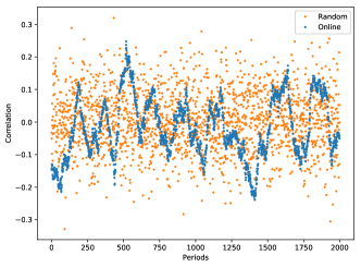
Figure 1: Correlations in time series of actions from classic Q-learning. For online correlations, the last 129 actions before each period are collected and the correlation between the first 128 and the last 128 actions is calculated (i.e., with time lag 1). For random correlations, two sequences with 128 actions each are randomly sampled from the recent 2000 actions before every period. We only report 2000 periods for one player during the learning process and data for another player share the same characteristics.

2.3 Deep Q-learning and random experience replay

Deep Q-learning can resolve the issues in classic Q-learning. First, deep Q-learning approximates $Q^{*}(s,a)$ with neural networks to improve the learning speed. Specifically, a Q-network $Q(s,a;\theta)$ with weights $\theta$ is a neural network function approximator of $Q^{*}(s,a)$. To train Q-networks, Mnih et al. (2015) consider a technique called experience replay (Lin, 1992), inspired by neuroscientific discoveries on brains. Briefly speaking, in each period $t$, the agent’s experience tuple $(s_{t},a_{t},r_{t},s_{t+1})$ is stored in a replay memory buffer with fixed length. When performing updates, Mnih et al. (2015) first sample tuples uniformly at random from the replay memory. We refer to this sample selection method as random experience replay. As shown in Figure 1, randomization can generate uncorrelated samples and break the strong temporal correlations. Moreover, tuples are likely to be selected for several times to improve the data efficiency. Next, the sampled experience tuples are used as a mini-batch in the minimization of certain loss functions (mean-square errors, Huber losses) on the differences in the Bellman equation (2.4). To be more precise, the optimal yet unknown values $r+\gamma\max_{a^{\prime}\in\mathcal{A}}Q^{*}(s^{\prime},a^{\prime})$ on the right hand side of (2.4) are replaced by the approximate but known values $r+\gamma\max_{a^{\prime}\in\mathcal{A}}Q(s^{\prime},a^{\prime};\theta^{-})$, where parameters $\theta^{-}$ are from some previous periods. The difference $\delta$ between two sides in (2.4) is defined as

$$\delta=Q(s,a;\theta)-\big{[}r+\gamma\max_{a^{\prime}\in\mathcal{A}}Q(s^{\prime},a^{\prime};\theta^{-})\big{]}.$$ (2.7)

Let ${\mathcal{L}}(\delta;\theta)$ be the loss function for a set of $\delta$, calculated from the mini-batch via random experience replay. Stochastic gradient methods are utilized to update $\theta$. After several episodes, $\theta^{-}$ is updated to the latest $\theta$. Therefore, unlike supervised learning, targets in deep Q-learning are not fixed and should be updated periodically. Algorithm 1 presents the details for deep Q-learning under a multi-agent setting. The Q-networks are trained with episodes and each episode contains certain periods or iterations.

For each agent $i=1,...,n$:

Initialize a replay memory $D^{i}$ with capacity $N$;

Initialize Q-network $Q^{i}$ with Calvano et al. (2020, Equation (8));

Initialize target Q-network $\hat{Q}^{i}$ with Calvano et al. (2020, Equation (8));

for episode $=1,...,M$ do

       Initialize a random state $s_{1}=((a^{1}_{0},...,a^{n}_{0}),...,(a^{1}_{-k+1},...,a^{n}_{-k+1}))$

       for period $t=1,...,T$ do

             For each agent $i$, with probability $1-\varepsilon_{t}$ select a greedy action $a^{i}_{t}=\arg\max_{a}Q^{i}(s_{t},a;\theta^{i})$; otherwise select a random action $a^{i}_{t}$

             Execute actions $(a^{1}_{t},...,a^{n}_{t})$ together and each agent observes all rewards $r_{i,t}$

             Set state $s_{t+1}=((a^{1}_{t},...,a^{n}_{t}),...,(a^{1}_{t-k+1},...,a^{n}_{t-k+1}))$

             Store transition $(s_{t},(a^{1}_{t},...,a^{n}_{t}),s_{t+1},(r_{1,t},...,r_{n,t}))$ in every $D^{i}$

             For each agent $i$, sample random mini-batch of transitions independently from $D^{i}$

             For each agent $i$, perform a gradient descent step on individual loss function with respect to weights $\theta^{i}$

            

       end for

      Every $C$ episodes, reset $\hat{Q}^{i}=Q^{i}$

end for

Algorithm 1 Multi-agent deep Q-learning with random experience replay

2.4 Discussions

In the single-agent setting, there are theoretical guarantees on the convergence for the two algorithms; see Watkins and Dayan (1992) for classic Q-learning and Fan et al. (2020) for deep Q-learning. However, in multi-agent Q-learning, when agents’ actions are regarded as part of state variables, the environment becomes non-stationary in the eyes of each agent. An agent’s policy depends on the states and therefore his rivals’ policies, which are also changing over periods by learning or experimenting under $\varepsilon$-greedy policies. Therefore, multi-agent Q-learning currently lacks general convergence results, due to the technical difficulties from non-stationarity. In practice, convergence is verified only ex-post. But luckily, the algorithms under the multi-agent setting investigated in this paper converge practically, possibly thanks to the relatively simple economic environment with low-dimensional state and action spaces.

Why do we select deep Q-learning instead of other variants of Q-learning? First, to destabilize algorithmic collusion, we must highlight that the key ingredient is random experience replay instead of deep neural networks. In our experiments, we adopt a neural network with only one hidden layer. The Q-network is by no means deep. It only speeds up the cell updates by learning $Q^{*}$ as a function. Later on, we will show that the results are robust to neural network designs in various aspects. However, random experience replay plays an essential role in breaking temporal correlations and improving data efficiency by reusing experience tuples more times. Second, since algorithmic collusion depends on the methodology that firms adopted, it is reasonable to consider some popular methods and assume the firms are using or exploring them. Moreover, compared with related works considering double deep Q-learning (Mellgren, 2020) and average reward deep Q-learning (Hettich, 2021), our model is parsimonious and guarantees a fair comparison.

In the following two sections, to facilitate the comparison with Calvano et al. (2020), we consider the same baseline model setting in Calvano et al. (2020) unless otherwise specified. Let number of agents $n=2$, marginal costs $c_{i}=1$, $b_{i}-c_{i}=1$, $b_{0}=0$, $\mu=0.25$, discount factor $\gamma=0.95$, number of feasible prices $m=15$, $\xi=0.1$, past prices length in state $k=1$. Let exploration rate $\beta=1\times 10^{-5}$, the middle value in Calvano et al. (2020). The learning rate for classic Q-learning is $\alpha=0.15$. Deep Q-learning uses the RMSprop optimizer with default parameters in PyTorch. In particular, the learning rate is $0.01$. Under this specification, the Bertrand equilibrium price $p^{N}$ is approximately 1.473 and the monopoly price $p^{M}$ is close to 1.925. The action space of feasible prices, is equally spaced and given as $\{1.43,1.47,1.51,...,1.95,1.99\}$ with a step size $0.04$. We encode the prices as action $0$ for price 1.43, action $1$ for price 1.47, etc. There are discretization errors and $p^{N},p^{M}$ are not exactly included in the action space. Besides, the state space has 225 elements.

Since certain features like fluctuating between two consecutive prices may be masked after averaging across different replications, we usually plot graphs with one particular session, unless otherwise specified, and describe common characteristics found among all sessions. We first destabilize the collusion and then recover the supra-competitive prices.

3 Destabilizing collusion

Temporal correlations have been illustrated in Figure 1. As indicated by the blue dots, trajectories of one player’s actions usually maintain local trends. In contrast, the randomly sampled actions have no obvious patterns and are close to uncorrelated. This difference turns out to be crucial in Mnih et al. (2015) for single-agent deep Q-learning. Originally, Mnih et al. (2015) conjectured that strong temporal correlations might lead to poor local minima or even divergence for the single-agent case. Notably, for multi-agent reinforcement learning, strong temporal correlations have certain benefits in maintaining stationarity for the environment. Rivals’ policies may not vary too rapidly. The agent can trust on recently observed experience tuples that are not obsolete. In contrast, multi-agent deep Q-learning with random experience replay can be highly non-stationary (Foerster et al., 2016; Leibo et al., 2017; Foerster et al., 2017). Therefore, random experience replay is totally disabled or carefully modified. Overall, these findings inspire us to destabilize algorithmic collusion by breaking temporal correlations with random experience replay. Since the economic environment is relatively simple compared with complicated computer gaming scenarios, the algorithms may still be viable to converge.

3.1 Classic Q-learning with random updating

Before moving into the experience replay setting, we further motivate the discussions by modifying the classic Q-learning algorithm. Instead of updating the cell corresponding to the current observed state, we randomly sample a previous experience tuple containing the action, state, and reward from a finite memory buffer and update that cell. This idea resembles the random experience replay technique but with a mini-batch size of one. Hereafter, we refer to this modification as the C-Random algorithm and the classic Q-learning in Section 2.2 as the C-Online algorithm. Although it may be economically unrealistic to force the agents to update an outdated cell instead of the current observation, we believe this modification provides a benchmark and explores the effect of random experience replay while keeping other factors unchanged. One can expect a cell is visited more frequently since randomization helps the C-Random algorithm escape from the local region in the current trajectory. However, a finite replay memory buffer prevents extensive random visits and guarantees the convergence.

In Figure 2, we observe that the C-Random algorithm shifts the long-run prices to the lower side. It indicates that breaking the temporal correlations can destabilize the collusion. However, supra-competitive prices still constitute a considerable proportion. One possible reason is the C-Random algorithm still updates one cell per period. An agent’s policy is not altered enough and can generate paths similar to the C-Online algorithm. Besides, we discover that the high prices ($\geq 1.91$) also appear more frequently after the convergence. Randomization may also enable the C-Random algorithm to explore these prices more extensively compared with the C-Online algorithm. Nevertheless, we highlight that the proportions of the lower prices increase more significantly.

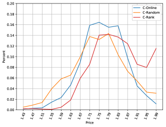
Figure 2: Distributions for long-run prices after convergence. The blue one replicates the outcomes in Calvano et al. (2020) with the classic Q-learning algorithm. The C-Random algorithm employs a replay memory with size 2250. The C-Rank algorithm is based on relative performance concerns and is detailed later in Section 4.2. We run each algorithm for 500 replications and collect the last 20 observations for each replication. The figure only plots data for one player since the other player has similar results.

3.2 Random experience replay

Motivated by the findings in Section 3.1, we explore the deep Q-learning framework with random experience replay (Mnih et al., 2015). For brevity, we refer to this renowned deep Q-learning Algorithm 1 as the D-Random algorithm. Consider the memory buffer size as 2000 and the mini-batch size as 128. Compared with computer science literature that regularly sets a buffer size to $10^{6}$ (Mnih et al., 2015; Zhang and Sutton, 2017), ours is much smaller, since action space and state space are significantly smaller. We assume two D-Random players use the same configuration for Q-networks, a fully-connected neural network with one hidden layer and hidden size $h=512$. To be more precise, the Q-network is a neural network $f:\mathbb{R}^{nk}\rightarrow\mathbb{R}^{m}$, from the state space to the Q-values for $m$ actions, given as

$$f(s)=W_{2}\sigma(W_{1}s+v_{1})+v_{2}.$$ (3.1)

$W_{1}\in\mathbb{R}^{h\times nk},v_{1}\in\mathbb{R}^{h},W_{2}\in\mathbb{R}^{m\times h}$, and $v_{2}\in\mathbb{R}^{m}$ are network weights. $\sigma(u)=\max\{u,0\}$ is the rectified linear unit (ReLU) activation function, applied element-wisely. Neural networks are commonly over-parameterized since the number of parameters greatly exceeds the input dimension $nk$. Initially, we set the action-value function implied by $f$ as given in Calvano et al. (2020, Equation 8), which can be achieved by setting $W_{1},W_{2},v_{1}=0$ and $v_{2}$ as Calvano et al. (2020, Equation 8). This is the main motive that we do not fix $v_{2}$ as zero. Robustness on the Q-network architecture is checked in Section 6.2. Our design does not have any fancy tricks and is somehow commonly used in deep learning literature. The Q-network is capable of generating greedy policies with flexible structures. However, our trained Q-networks consistently yield constant greedy policy matrices.

Following Mnih et al. (2015), we train the Q-networks for a given length of episodes and do not specify convergence criteria like Calvano et al. (2020). Greedy policy matrices under deep Q-learning usually fluctuate between several consecutive prices after convergence, which is illustrated later in Figure 3. We fix the number of episodes to 2000. Each episode contains 500 periods. Table 1 reports descriptive statistics of the long-run prices during the last episode for two players, labeled as Player 1 and Player 2. Besides, each episode yields 500 greedy policy matrices for one player. However, each matrix turns out to be constant. Thus, Table 1 also presents statistics for these matrices. Both players select prices 1.47 and 1.51 more frequently. The highest is 1.63 with a relatively low proportion. Two players do not charge the same all the time, but their choices are close to each other. These characteristics reported in Table 1 are pervasive in all replications we have run.

Price	1.43	1.47	1.51	1.55	1.59	1.63
Percent (Player 1)	17.4%	19.8%	38.0%	17.4%	5.8%	1.6%
Percent (Player 2)	16.8%	25.0%	33.0%	19.4%	5.0%	0.8%
Relative price	Player 1 $>$ Player 2		Player 1 $=$ Player 2		Player 1 $<$ Player 2
Percent	40.0%		24.0%		36.0%

Table 1: Statistics of long-run prices for two D-Random players during the last episode.

Figure 3 further illustrates the evolution of selected prices during the entire training with several quantiles. In the beginning, the proportion of prices not exceed 1.51 is only $20\%$. Since there are 15 feasible prices and three of them satisfy this threshold, the starting percentage is not far from the equally assigned probabilities. The proportion rises steadily and contributes to 80% eventually. Sharp fluctuations during the learning process may be due to random exploration. Remarkably, D-Random algorithms seldom select extremely high prices for the whole training period. The initial greedy policies select price 1.59 under the initialization given in Calvano et al. (2020, Equation 8). Importantly, we find the results are robust to the methods of initialization; see Section 6.5. If set the initial greedy choice to the highest feasible price, the outcomes still remain close to the Bertrand equilibrium. Figure 3 shows that the highest selected prices for each episode decrease slightly. Moreover, the frequencies for these highest prices are typically low. Table 1 provides details for the last episode. High prices vanish quickly under the D-Random algorithms. Finally, the most frequent prices fluctuate between 1.47 and 1.51, close to the one-shot Bertrand equilibrium.

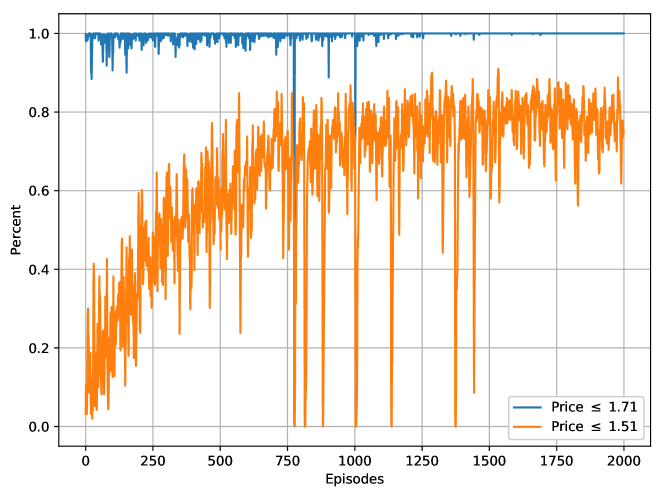
(a) Percents of prices not exceed 1.51 and 1.71

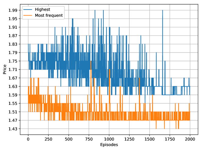
(b) The highest and the most frequent prices

Figure 3: Evolution of selected prices in each episode. Only data for one player are shown. Another player exhibits the similar pattern.

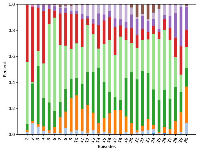
(a) The first 30 episodes

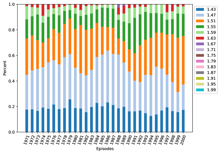
(b) The last 30 episodes

Figure 4: Distributions for selected prices in each episode. For simplicity, only the first and the last 30 episodes are reported.

Figure 4 demonstrates the frequencies of prices during the start and the end of the learning process. Figure 4 agrees with Figure 3 on the trend of prices within several thresholds. Figure 4 also shows the detailed percentage for the highest and the most frequent prices during the last several episodes, consistent with Figure 3. From Table 1, Figure 3 and 4, we can conclude that the D-Random algorithm obtains prices close to the Bertrand equilibrium and destabilizes the algorithmic collusion discovered under the C-Online method. Moreover, we also adopt the same idea in Calvano et al. (2020): Step in after convergence and exogenously force one player to defect. Check for any punishments from the rivals. We observe that both players immediately return to the long-run prices in the next period after the deviation. The forced deviation has an almost zero impact on the outcomes. It is reasonable since the deviation lasts only for one period and the agents sample their experiences randomly from replay memories. The weighting on the deviation is significantly low. Moreover, the constant greedy policies also imply that there is no reward-punishment scheme learned by the D-Random algorithm.

Compared with the C-Random algorithm in Section 3.1, the D-Random algorithm further breaks the temporal correlations. Fully-connected neural networks (3.1) do not learn the order of samples from mini-batches. A moderate batch size also ensures the sampled experience tuples are near uncorrelated (Fan et al., 2020). Moreover, Q-networks update greedy policies for all cells as a whole. This characteristic has advantages and also disadvantages, compared with C-Online and C-Random algorithms. One can expect Q-networks are more efficient. However, imposing structures on Q-networks may implicitly restrict the domains of Q-values. Although neural networks are universal function approximators (Cybenko, 1989), the practical implementation may not satisfy all theoretical requirements. On the other hand, we did not have convergence issues in two-agent D-Random algorithms, in contrast to Foerster et al. (2016, 2017); Leibo et al. (2017). One possible explanation is, non-stationarity is weak under a relatively simplified economic environment.

4 Recovering collusion

4.1 Online experience replay

A natural question is, with deep Q-learning, is it still possible to recover algorithmic collusion or at least significantly higher prices than the Bertrand equilibrium? Random experience replay assigns equal weights on all experience tuples in the memory buffer. However, agents may have certain preferences and do not always pick up data randomly. The first idea is online experience replay. It resembles the C-Online algorithm and uses the most recent data in the memory buffer. For the fairness of comparison, we still fix the same mini-batch size as 128. The only difference is the mini-batch contains exactly the latest 128 experience tuples. We refer to deep Q-learning with online experience replay as the D-Online algorithm. One can expect that temporal correlations are restored moderately under this setting. Experiments suggest that online experience replay raises, albeit slightly, the price levels to be above 1.51. Compared with Figure 3, only the sampling method is modified. We can attribute this trend towards supra-competitive prices to the temporal correlations within the recent samples. Another distinction is each D-Online player only selects two, or even one, price(s) after convergence. Compared with six possible long-run prices in Table 1, online experience replay greatly stabilizes the training progression.

However, the D-Online algorithm does not obtain prices close to 1.78 as in Calvano et al. (2020). Clearly, Q-networks do not detect the order of samples in the mini-batch. A natural extension in the future is to adopt other architecture such as LSTM or RNN. One can also conjecture that reducing the mini-batch sizes and chunking the data to feed the Q-networks sequentially will strengthen the local dependencies. However, a small mini-batch size usually makes the learning process unstable, since not enough information is passed to the network during a single period. Indeed, with a small mini-batch size like 8, algorithms select much more prices, compared with merely two choices for each player before.

4.2 Rank experience replay

To incorporate relative performance concerns, we assume each firm only memorizes the periods when its profit does not exceed that of the rivals. Periods when it overtakes the competitors are dismissed. This assumption may sound extreme, but it amplifies the effects of relative performance. We consider the simplest case with two firms. The replay memory buffer of each firm only contains tuples that the reward is lower than or equal to the rival. As mentioned previously, one firm can observe competitors’ actions and profits. However, all firms do not know the underlying demand and reward mechanism. To be more precise, they are unaware that the demand is calculated with the logit model (2.1), and selecting a lower price than that of the competitor can yield a higher reward. They have to discover any patterns about the rewards totally from the observed data. Recall an experience tuple is given as $(s_{t},a_{t},r_{t},s_{t+1})$. In our symmetric economic environment, rank experience replay makes Player 1 merely focus on the tuples with reward $r_{1,t}\leq r_{2,t}$. Under these scenarios, the selected price $a^{1}_{t}\geq a^{2}_{t}$. However, there is no relative constraint on the current state $s_{t}$. Thus, rank experience replay is still viable to visit arbitrary states.

Suppose we still randomly sample from rank replay memory buffers. We call deep Q-learning with rank experience replay the D-Rank algorithm. Remarkably, the D-Rank algorithm quickly converges to supra-competitive prices; see Figure 5. Both players select the same long-run price and therefore are ranked the same. It is the equilibrium when firms are also concerned with rankings. Nevertheless, only high prices exist. No reward-punishment mechanism is detected as in Calvano et al. (2020). The greedy policy matrices are still constant for all states. If one firm defects for one period, both immediately restore the pre-deviation price in the following period. The defection incurs no punishment from the rival at all.

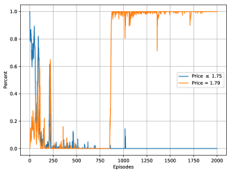
Figure 5: Rank experience replay. Fractions with prices below 1.79 drop quickly. The strategies fix at 1.79 after relatively short numbers of episodes. Both players select 1.79. Graphs for another player omitted.

Why D-Rank algorithms yield supra-competitive prices? Note that under the baseline economic environment, a lower price generates a higher profit than the rivals. Nevertheless, if both firms choose lower prices, they will earn lower profits. There could have been price wars. Impressively, D-Rank algorithms avoid this Prisoner’s dilemma and maximize the aggregate profits even without communications. The absence of strong temporal correlations does not dominate the advantages of exploring ranking information. We explain the dynamics of D-Rank algorithms with the trade-off between exploitation and exploration. On the one hand, the D-Rank method improves the exploitation by only concentrating on the regions where the previous Q-network has failed to achieve a better ranking and selected a price higher than that of the competitor. Filtering tuples by relative performance facilitates the coordination between firms and prevents uniform sampling from contaminating the learning process. Experience tuples with relatively higher prices consistently receive more attention. We emphasize that “higher” prices here are relative to competitors’. These prices may not be high enough in the action space to reach supra-competitive levels. On the other hand, random exploration introduces tuples with arbitrarily chosen prices, yet still should not be lower than competitors’ if pushed into memories. Algorithms detect higher profits in some experiences and optimize the parameters to adjust the policies. In general, D-Rank algorithms do not keep raising prices monotonically. Indeed, Figure 5 shows that prices in episodes between 250 and 750 are higher than the final limit of 1.79.

There are several remarks on the D-Rank algorithm. First, Calvano et al. (2020) raises an open question about the time needed to reach collusive strategies. We consistently observe that rank experience replay accelerates the training progression and converges much faster. In particular, Figure 5 clearly shows the supra-competitive prices can be achieved with merely 750 episodes with 500 periods in each episode. If we ignore the longer time required in training neural networks and make a comparison with 850,000 periods reported in Calvano et al. (2020) under the same baseline environment, the time scale is reduced quite significantly. Second, as a general remark, we are in an age of big data. However, more data do not automatically imply more advantages. Obsolete data may contaminate the learning process and lead to worse outcomes for the agents (however, better outcomes for the consumers in this special case). By ignoring certain abundant data, algorithms could obtain better results.

In the same spirit, we incorporate relative performance with classic Q-learning and refer to it as the C-Rank algorithm. A classic agent only updates the most recent cell when his profit does not exceed the rival. If underperformance occurs in the current period, then it reduces to the updating in the original C-Online algorithm. If the current period witnesses an outperformance, then the latest cell with underperformance is updated. As expected, the C-Rank algorithm also shifts the long-run prices to higher levels than C-Online algorithms. See Figure 2 for a comparison between C-Online, C-Random, and C-Rank algorithms.

Not all agents are concerned about relative performance. If a D-Random player meets a D-Rank competitor, we find that the long-run prices are between outcomes of two D-Random players (Figure 3) and two D-Rank players (Figure 5). Commonly, the long-run prices oscillate in different regions for the two players, shown in Figure 6. The D-Rank player consistently selects a higher price than his D-Random competitor. There are more cases of player heterogeneity in the next section.

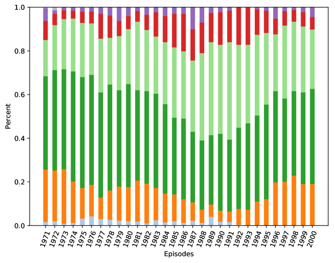
(a) The D-Rank player

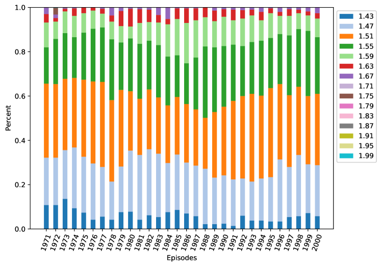
(b) The D-Random player

Figure 6: Distributions for long-run prices when deep players have heterogeneous concerns on relative performance. In the last episode, the D-Rank player selects price 1.55 mostly, while the D-Random rival selects 1.51 more commonly. During 65.6% of the last episode, the D-Rank player sets a higher price than his competitor.

5 Heterogeneous players

For most scenarios in the previous sections, we have assumed two homogeneous players. Since collusion is a matter of coordination, a natural concern is two players adopting different learning algorithms and/or different economic considerations. There are numerous combinations. To ease the exposition and highlight the roles of random and rank experience replay, we only consider three particular cases: a C-Online player and a D-Random player; a C-Online player and a D-Rank player; a C-Rank player and a D-Rank player.

5.1 C-Online player and D-Random player

Suppose one player uses the C-Online algorithm and another player adopts the D-Random algorithm instead. Overall, convergence is more difficult under this situation. We have observed sessions with prices fluctuating over a wide range, with no clear sign of convergence. When converged, the long-run prices for the D-Random player are still more volatile, as plotted in Figure 7 for the entire training process of a particular session. However, a comparison between Figure 7 and Figure 3 do indicate the possibility of high prices under heterogeneous players. During the last episode, the D-Random player consistently chooses price 1.59, while the greedy policy matrix for the C-Online player selects prices in cycle $1.79\rightarrow 1.63\rightarrow 1.71\rightarrow 1.59\rightarrow 1.79\rightarrow\cdots$, detailed in Figure 7. The upper half of the matrix generally has lower prices (deeper colors), while the lower half has higher prices (lighter colors). When we exogenously force the D-Random player to defect, the greedy policies for both players are unchanged. Figure 7 indicates that if the D-Random player cuts his price, then the C-Online player will also cut his price, which is the punishment of deviations. It agrees with the reward-punishment scheme in Calvano et al. (2020). Besides, the deep player still uses a constant greedy policy matrix, even when the rival is more flexible.

The high prices raise a tricky question for regulations on algorithmic collusion. Apparently, firms cannot escape the responsibility of collusion by attributing it completely to the algorithms. Suppose we agree that the two firms with C-Online algorithms both are liable for algorithmic collusion. In contrast, if they employ D-Random algorithms, then the price is competitive and close to the Bertrand equilibrium. However, when a C-Online player appears, the prices are raised significantly again. We may agree that the C-Online player is liable for the collusive strategies. But, should the D-Random player under the heterogeneous setting also take some responsibilities? If we think the D-Random player is liable in the same sense as the C-Online player, then the D-Random player may have the following complaint. If the C-Online competitor also uses his D-Random algorithm, then there is no collusion at all. If we think the D-Random player is innocent, he definitely benefits from the raised prices and makes more profits. If we think the D-Random player is partially liable, to what extent should we punish him? How can we judge the D-Random agent, a fallen angel, is acting voluntarily or involuntarily? These questions are left open for further discussions.

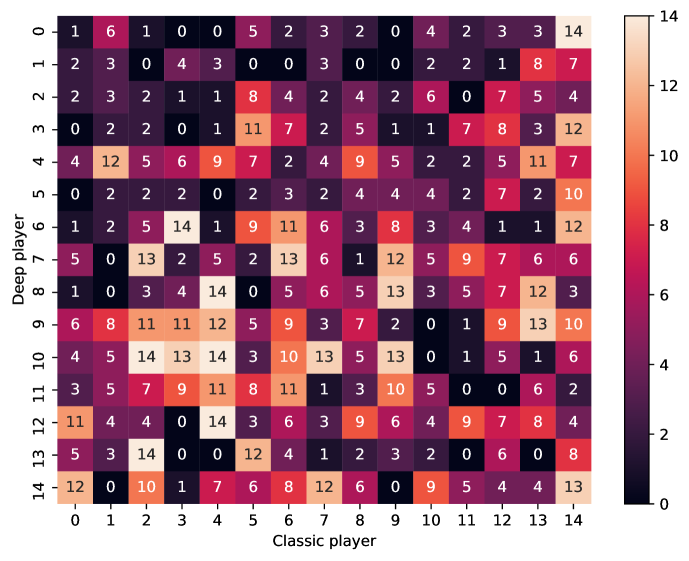
(a) Greedy policy for the C-Online palyer

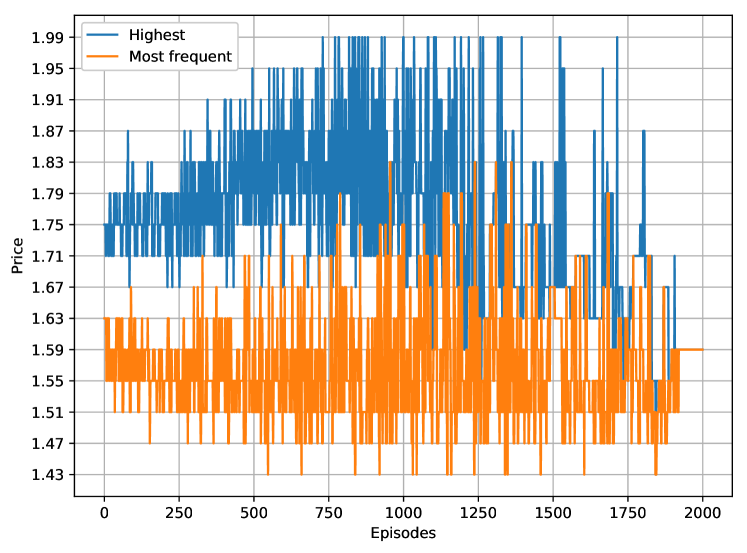
(b) The D-Random player

Figure 7: The left subgraph shows the greedy policy matrix of the C-Online player during the last episode. Recall the prices are encoded consecutively as follows: 0 for price 1.43, 1 for price 1.47, etc. The horizontal axis stands for the previous choice of the C-Online player. The vertical axis is for the D-Random player. The right subgraph plots the highest and the most frequent prices chosen by the D-Random player in the same way as in Figure 3.

5.2 C-Online player and D-Rank player

Notably, rank experience replay also stabilizes the collusion under heterogeneous players. First, consider a C-Online player with a D-Rank player. Fluctuations in the D-Rank player’s actions are reduced. But in general, we cannot form a solid conclusion that prices of D-Rank players are higher or lower than those of D-Random players. The main reason is high variances present when a D-Random player meets a C-Online player, as depicted in Figure 7. It weakens the power of the comparison.

5.3 C-Rank player and D-Rank player

Furthermore, we assume both players are concerned about rankings. The algorithms converge at a relatively short time scale, similar to Figure 5, with supra-competitive prices. However, the punishment of defection vanishes, as indicated by a comparison between Figure 7 and Figure 8. Imagine the D-Rank player reduces the price to be below 1.47 (action 1), the C-Rank player will still keep his price at a high level. In contrast, Figure 7 will tell the C-Online player to cut the price.

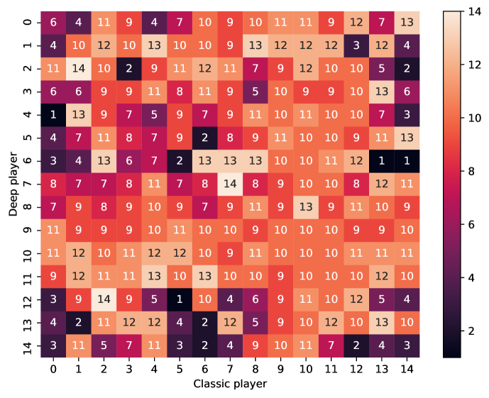
(a) The C-Rank player

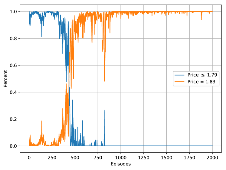
(b) The D-Rank player

Figure 8: C-Rank player and D-Rank player. The left subgraph illustrates the greedy policy of the C-Rank player. Both players select price 1.83, labeled as action 10, after convergence. The right subgraph indicates a rapid convergence for the D-Rank player, similar to Figure 5.

To identify the factors contributing to this elimination of punishment, we have also checked the greedy policies for another two cases: two C-Rank players or a C-Online player with a D-Rank player. However, no similar effect is detected. We speculate the reasons as follows. Deep Q-learning tends to select a constant greedy policy, under many scenarios. But the D-Random player in Figure 7 is volatile and the classic player cannot detect the constant policy. When both players consider rankings, the algorithms are the most stable. The classic player has successfully anticipated this pattern and believes the deep player will immediately return to the pre-deviation price in the next period. To validate this conjecture, we consider two classic players. Force one player to select a fixed price, for example, 1.83, with a time-increasing probability of $1-\varepsilon_{t}$. The $\varepsilon$-greedy policy is adopted with a probability of $\varepsilon_{t}$. This player tries to mimic the behaviors of a D-Rank player. His competitor is a typical C-Rank player. We manage to approximately replicate features in the greedy policy shown in Figure 8. As depicted in Figure 9, the experiment also eliminates the punishment from the C-Rank player. In this design, the classic player must adopt rank experience replay, while it does not matter whether the player mimicking a constant policy adopts or not.

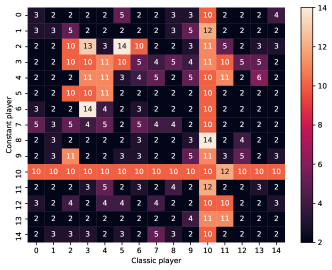
Figure 9: Greedy policy for the C-Rank player, facing another classic player using a constant policy gradually. We set the constant policy as price 1.83 (action 10). This figure resembles Figure 8 in the sense that it eliminates the punishment for the defection of the constant player.

6 Robustness

There are numerous hyper-parameters and combinations. To ease the exposition, we only consider one factor each time and fix most others as given under the baseline setting.

6.1 Asymmetric firms

Asymmetry reduces the average profit gain (Calvano et al., 2020). Moreover, another concern is that the interaction between asymmetry and rank experience replay. We focus on the cost asymmetry, reported in Table 2. D-Random algorithms still perfectly inhibit the algorithmic collusion and obtain the closest price pair to the Bertrand equilibrium. Similar to Calvano et al. (2020), the collusion under C-Online algorithms is reduced only by a limited extent. Remarkably, Table 2 discloses the mechanism and a drawback of rank experience replay. For both C-Rank and D-Rank algorithms, the more efficient firm, Player 2 with a lower marginal cost, always charges a higher price than the less efficient rival. This pattern is distinct from all other algorithms and theoretical prices. In a two-agent setting, rank experience replay makes competitors concentrate on the borderline where rewards are the closest to each other and they could achieve similar rankings, if possible. Price pairs $(1.55,1.60)$ and $(1.65,1.75)$ are located near the borderline. The C-Rank algorithm traps at a lower price pair, compared with the D-Rank case. Trajectories of D-Rank algorithms show that the prices are not moving monotonically. They raise and drop for several turns, while the lower bound is increasing and fixes at the long-run prices after convergence. It reflects the tight games between two players with relative profits in mind. Besides, since theoretical prices in Table 2 enlarge the action space, it also verifies the robustness of action spaces.

Strategy	Bertrand	Monopoly	C-Online	C-Rank	D-Random	D-Rank
Player 1	1.372	2.198	1.95$\rightleftarrows$1.70	1.55	1.40	1.65
Player 2	1.204	1.698	1.70	1.60	1.25	1.75

Table 2: Cost asymmetry. The marginal cost for Player 2 changes to $0.5$. Action space is enlarged as $\{1.15,1.20,...,2.30,2.35\}$ for both players. Other parameters are the same as in the baseline setting. The first two columns are theoretical prices.

6.2 Q-networks

Designing neural networks usually needs expertise and careful tuning. There are many choices that might look arbitrary, including depth (the number of hidden layers), width (the number of neurons in each layer), activation functions, and other techniques embracing dropout, layer normalization, etc. It is impossible to test all the designs. Although the universal approximation result (Cybenko, 1989) guarantees sufficiency even with a single hidden layer, one conventional wisdom, yet debatable, is that a deeper network is better than a wider one (Eldan and Shamir, 2016). Since our baseline model only has one hidden layer, a natural concern is whether more hidden layers could discover the collusive strategies. We have tested a deeper network with 10 hidden layers and a smaller width ($h=16$). The long-run prices do not show any significant difference with the Bertrand equilibrium achieved. Moreover, the greedy policies remain constant for both players.

Another concern is the bias term $v_{2}$ in the last layer. Some works may not use the final bias term (Fan et al., 2020). If it is activated, the initialization of weights should be done carefully (Karpathy, 2019). As explained previously, if the last bias term is adopted, then it is easy to follow the initialization in Calvano et al. (2020). Otherwise, the inverse problem of finding the exact network weights for given greedy policies is nontrivial. The last bias term uniformly shifts the Q-value functions regardless of the states. If the vector $v_{2}$ is larger than the first term in (3.1) by several orders of magnitude, then the greedy policy is more likely to be constant. However, even when we fix $v_{2}=0$, the network still produces constant greedy policies. Another important observation is, after many iterations, the algorithm usually learns the term $v_{2}$ only, while fixing other weights unchanged. It stabilizes the training progression, while it may also restrict the structures of Q-value functions. Nevertheless, it is chosen by the algorithm automatically.

Mellgren (2020) reported that double deep Q-learning also cannot learn to punish defections. In contrast, Hettich (2021) managed to learn a reward-punishment scheme with an average reward formulation. However, Hettich (2021) adopted many different designs, compared with this paper and Mellgren (2020). It is then left open to find which factor is crucial for the reward-punishment mechanism.

6.3 Learning rate

Learning rate	$10^{-3}$	$10^{-4}$	$10^{-5}$	$10^{-6}$	$10^{-7}$
D-Random	$(1. 51,1.49)^{*}$	(1.51, 1.55)	(1.63, 1.59)	1.67	1.59
D-Rank	1.75	1.83	1.67	1.67	1.59

Table 3: Long-run prices under different learning rates. Prices in parentheses are for Player 1 and 2 respectively. For simplicity, only one value is reported if both players select the same price. The marked cell for D-Random algorithm with $10^{-3}$ gives the average values, since each player selects two prices. For other cells, each player charges one price only.

Learning rate is an important hyper-parameter. For classic Q-learning, we adopt the same value as in Calvano et al. (2020). For deep Q-learning, we use the default value 0.01 for the RMSprop optimizer in PyTorch. For robustness check, Table 3 provides the deep Q-learning results with different learning rates. A smaller learning rate makes the training more stable but also much slower. Indeed, the algorithms only select one or two prices, in contrast to Table 1. $10^{-3}$ and $10^{-4}$ perform better than the default value. $10^{-7}$ is too small for the training and greedy policies are the initial ones. We observe that, at first, decreasing learning rate makes the D-Random algorithm obtain higher prices. Players’ policies change slower and it prevents random experience replay from destroying the coordination. The highest price obtained by the D-Random algorithm is 1.67, under the learning rate $10^{-6}$. However, it is still much lower than the supra-competitive price (1.78) obtained in Calvano et al. (2020). More importantly, the D-Random algorithm with a learning rate $10^{-6}$ is sensitive to the Q-matrix initialization. Long-run prices are close to the initial choices, no matter high or low.

6.4 Memory buffer sizes and mini-batch sizes

Experience replay introduces a new hyper-parameter, memory buffer size. Zhang and Sutton (2017) provides an empirical study on the importance of buffer size and finds it is task-dependent. Both a small and a large buffer size can hurt the training process. We have also considered a large one as $2\times 10^{5}$. Deep Q-learning with random or rank experience replay tends to be robust. Algorithms with a large or a moderate size do not exhibit significant differences in the results.

On the other hand, the effect of mini-batch sizes has been mentioned concretely in online experience replay. Similarly, for random experience replay, a smaller mini-batch size like eight also makes the training progression volatile. However, the long-run prices still fluctuate near the Bertrand equilibrium.

6.5 Initialization

In the baseline setting, the Q-matrix is initialized under the assumption that one agent’s opponents initially select any actions uniformly at random (Calvano et al., 2020), regardless of the state. The greedy policy under this specification is constant. It consistently charges a price of 1.59 (action 4) for any state. However, it is debatable on which initialization is optimal or truly non-informative. Therefore, we conduct a robustness check on several initialization methods.

Initialization	Baseline	Q = 0	Random	Q = 19	Topmost
D-Random	Bertrand	Bertrand	Bertrand	Bertrand	Bertrand
D-Rank	High	High	High	High	High
C-Rank	High	Upper bound	Upper bound	High	Volatile

Table 4: Convergence results under different initialization. The action space is enlarged to $\{1.43,1.47,...,2.15,2.19\}$ with 20 actions, equally spaced with step size 0.04. The upper bound is significantly higher than the monopoly price.

Table 4 considers five methods. The first method, baseline, is from Calvano et al. (2020, Equation 8). The second sets the Q-matrix as zero. Sutton (1996); Zhang and Sutton (2017) documented that zero initial Q-values encourage exploration. The third random method is implemented differently for the classic and deep setting. Classic algorithms uniformly sample Q-matrix entries from $[0,1)$, while deep ones initialize Q-network weights randomly. The fourth method sets a large constant for the Q-matrix. The last method called “topmost” sets the Q-matrix to be zero, except that entries for the highest price are a large constant. Therefore, the initial greedy policy selects the highest price.

Deep players with random or rank experience replay are robust to all the initialization methods. “Bertrand” refers to the convergence close to the competitive price 1.47. “High” means prices are supra-competitive. In particular, D-Random algorithms still converge to the Bertrand equilibrium when the initial policies select the highest price.

C-Rank algorithms are sensitive to Q-matrix initialization. “Upper bound” means the algorithms simply converge to the highest feasible values, even above the monopoly prices. “Volatile” represents the algorithms converge to long circles with both low and high prices presented. Distinct from deep Q-learning, C-Rank algorithms tend to be trapped by the priori information given in the initialization. For example, neighbor cells in the greedy policies can have very distinct values after convergence. Classic Q-learning has already demonstrated strong temporal correlations. Rank experience replay further increases the frequencies of tuples with higher prices than competitors. Therefore, C-Rank algorithms might be prone to get stuck in poor local maxima or even diverge.

7 Conclusions

This paper utilizes an experimental approach to understand algorithmic collusion. A crucial open question is theoretical guarantees on the convergence to collusive or competitive strategies and the convergence rates under a multi-agent setting. Another problem left for future research is that fully-connected neural networks consistently learn constant greedy policies. However, the rationality is currently unclear. More efforts are needed in exploring other architectures of deep networks. Finally, the experiment assumes a relatively simplified economic environment. One direction is to consider more realistic settings or create innovative approaches to study the topic with empirical data.

References

- Assad et al. (2020) Assad, S., Clark, R., Ershov, D., and Xu, L. (2020). Algorithmic pricing and competition: Empirical evidence from the German retail gasoline market. Working Paper. https://ssrn.com/abstract=3682021.
- Bizjak et al. (2016) Bizjak, J., Kalpathy, S. L., Li, Z. F., and Young, B. (2016). The role of peer firm selection in explicit relative performance awards. Working Paper. https://ssrn.com/abstract=2833309.
- Calvano et al. (2020) Calvano, E., Calzolari, G., Denicolò, V., Harrington, J. E., and Pastorello, S. (2020). Protecting consumers from collusive prices due to AI. Science, 370(6520), 1040–1042.
- Calvano et al. (2020) Calvano, E., Calzolari, G., Denicolò, V., and Pastorello, S. (2020). Artificial intelligence, algorithmic pricing, and collusion. American Economic Review, 110(10), 3267–97.
- Casas-Arce and Martinez-Jerez (2009) Casas-Arce, P. and Martinez-Jerez, F. A. (2009). Relative performance compensation, contests, and dynamic incentives. Management Science, 55(8), 1306–1320.
- Cybenko (1989) Cybenko, G. (1989). Approximation by superpositions of a sigmoidal function. Mathematics of Control, Signals and Systems, 2(4), 303–314.
- Eldan and Shamir (2016) Eldan, R. and Shamir, O. (2016). The power of depth for feedforward neural networks. In Feldman, V., Rakhlin, A., and Shamir, O. (Eds.), Proceedings of the 29th Conference on Learning Theory, volume 49, (pp. 907–940).
- Ezrachi and Stucke (2016) Ezrachi, A. and Stucke, M. E. (2016). Virtual competition. Oxford University Press.
- Fan et al. (2020) Fan, J., Wang, Z., Xie, Y., and Yang, Z. (2020). A theoretical analysis of deep q-learning. In Bayen, A. M., Jadbabaie, A., Pappas, G. J., Parrilo, P. A., Recht, B., Tomlin, C. J., and Zeilinger, M. N. (Eds.), Proceedings of the 2nd Annual Conference on Learning for Dynamics and Control, volume 120, (pp. 486–489).
- Fisher et al. (2018) Fisher, M., Gallino, S., and Li, J. (2018). Competition-based dynamic pricing in online retailing: A methodology validated with field experiments. Management Science, 64(6), 2496–2514.
- Foerster et al. (2017) Foerster, J., Nardelli, N., Farquhar, G., Afouras, T., Torr, P. H. S., Kohli, P., and Whiteson, S. (2017). Stabilising experience replay for deep multi-agent reinforcement learning. In Precup, D. and Teh, Y. W. (Eds.), Proceedings of the 34th International Conference on Machine Learning, volume 70, (pp. 1146–1155).
- Foerster et al. (2016) Foerster, J. N., Assael, Y. M., de Freitas, N., and Whiteson, S. (2016). Learning to communicate with deep multi-agent reinforcement learning. In Lee, D. D., Sugiyama, M., von Luxburg, U., Guyon, I., and Garnett, R. (Eds.), Advances in Neural Information Processing Systems 29, (pp. 2137–2145).
- Hansen et al. (2020) Hansen, K., Misra, K., and Pai, M. (2020). Algorithmic collusion: Supra-competitive prices via independent algorithms. Marketing Science.
- Hao et al. (2011) Hao, S., Jin, Q., and Zhang, G. (2011). Relative firm profitability and stock return sensitivity to industry-level news. The Accounting Review, 86(4), 1321–1347.
- Hastie et al. (2009) Hastie, T., Tibshirani, R., and Friedman, J. (2009). The elements of statistical learning: Data mining, inference, and prediction. Springer.
- Hettich (2021) Hettich, M. (2021). Algorithmic collusion: Insights from deep learning. Working Paper. https://ssrn.com/abstract=3785966.
- Johnson et al. (2020) Johnson, J., Rhodes, A., and Wildenbeest, M. R. (2020). Platform design when sellers use pricing algorithms. Working Paper. https://ssrn.com/abstract=3753903.
- Karpathy (2019) Karpathy, A. (2019). A recipe for training neural networks. https://karpathy.github.io/2019/04/25/recipe/.
- Klein (2019) Klein, T. (2019). Autonomous algorithmic collusion: Q-learning under sequential pricing. Working Paper. https://ssrn.com/abstract=3195812.
- Kokkoris (2020) Kokkoris, I. (2020). A few reflections on the recent caselaw on algorithmic collusion. Working Paper. https://ssrn.com/abstract=3665966.
- Lazear and Rosen (1981) Lazear, E. P. and Rosen, S. (1981). Rank-order tournaments as optimum labor contracts. Journal of Political Economy, 89(5), 841–864.
- Leibo et al. (2017) Leibo, J. Z., Zambaldi, V. F., Lanctot, M., Marecki, J., and Graepel, T. (2017). Multi-agent reinforcement learning in sequential social dilemmas. In Larson, K., Winikoff, M., Das, S., and Durfee, E. H. (Eds.), Proceedings of the 16th Conference on Autonomous Agents and MultiAgent Systems, (pp. 464–473).
- Lin (1992) Lin, L.-J. (1992). Self-improving reactive agents based on reinforcement learning, planning and teaching. Machine Learning, 8(3-4), 293–321.
- Mellgren (2020) Mellgren, F. (2020). Tacit collusion with deep multi-agent reinforcement learning. Master Thesis, Stockholm School of Economics.
- Miklós-Thal and Tucker (2019) Miklós-Thal, J. and Tucker, C. (2019). Collusion by algorithm: Does better demand prediction facilitate coordination between sellers? Management Science, 65(4), 1552–1561.
- Mnih et al. (2015) Mnih, V., Kavukcuoglu, K., Silver, D., Rusu, A. A., Veness, J., Bellemare, M. G., Graves, A., Riedmiller, M., Fidjeland, A. K., Ostrovski, G., et al. (2015). Human-level control through deep reinforcement learning. Nature, 518(7540), 529–533.
- Schaul et al. (2016) Schaul, T., Quan, J., Antonoglou, I., and Silver, D. (2016). Prioritized experience replay. In Bengio, Y. and LeCun, Y. (Eds.), 4th International Conference on Learning Representations.
- Sutton (1996) Sutton, R. S. (1996). Generalization in reinforcement learning: Successful examples using sparse coarse coding. In Touretzky, D., Mozer, M. C., and Hasselmo, M. (Eds.), Advances in Neural Information Processing Systems, volume 8. MIT Press.
- Sutton and Barto (2018) Sutton, R. S. and Barto, A. G. (2018). Reinforcement learning: An introduction. MIT press.
- Waltman and Kaymak (2008) Waltman, L. and Kaymak, U. (2008). Q-learning agents in a Cournot oligopoly model. Journal of Economic Dynamics and Control, 32(10), 3275–3293.
- Watkins and Dayan (1992) Watkins, C. J. and Dayan, P. (1992). Q-learning. Machine Learning, 8(3-4), 279–292.
- Watkins (1989) Watkins, C. J. C. H. (1989). Learning from delayed rewards. PhD thesis, King’s College, University of Cambridge.
- Zhang and Sutton (2017) Zhang, S. and Sutton, R. S. (2017). A deeper look at experience replay. arXiv preprint arXiv:1712.01275.