Taylor Dispersion in Thin Liquid Films of Volatile Mixtures: A Quantitative Model for Marangoni Contraction
Abstract
The Marangoni contraction of sessile droplets occurs when a binary mixture of volatile liquids is placed on a high-energy surface. Although the surface is wetted completely by the mixture and its components, a quasi-stationary non-vanishing contact angle is observed. This seeming contradiction is caused by Marangoni flows that are driven by evaporative depletion of the volatile component near the edge of the droplet. Here we show that the composition of such droplets is governed by Taylor dispersion, a consequence of diffusion and strong internal shear flow. We demonstrate that Taylor dispersion naturally arises in a self-consistent long wave expansion for volatile liquid mixtures. Coupled to diffusion limited evaporation, this model quantitatively reproduces not only the apparent shape of Marangoni-contracted droplets, but also their internal flows.
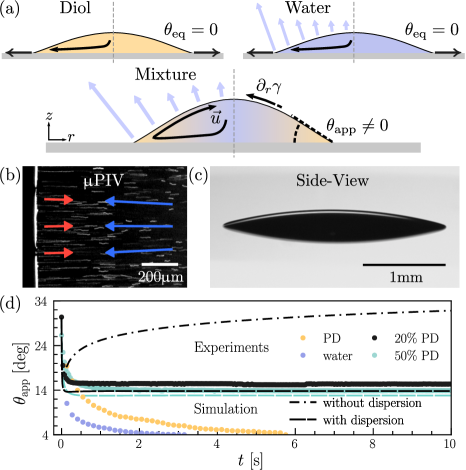
Wetting and dewetting of volatile liquid mixtures on solid surfaces is abundant in natural phenomena and technological applications [1, 2, 3, 4, 5]. Many examples are found in everyday life situations, for instance, biological fluids such as blood [6] and tears [7], inks for inkjet printing [8, 9], and paints for artistic techniques [10, 11]. Marangoni contraction is a prime example that gained significant attention recently, not least motivated by its applications in printing and semiconductor processing [12, 13, 14, 15, 16, 17, 18, 19]: Volatile liquids seemingly dewet from high energy surfaces over which they spread if evaporation was suppressed, see Fig. \IfSubStrfig:FIG1eq:(1)1 (a, c). Evaporation causes compositional [12, 13, 14, 17, 18] or thermal [19] gradients, inducing an inward Marangoni flow which contracts the droplet. The opposite case may lead to Marangoni spreading and contact-line instabilities [20, 21, 22]. The dynamics of contact lines is a multi-scale problem which involves both macroscopic hydrodynamics and molecular interactions [4, 23]. Thus, while multi-component liquids with pinned contact lines are understood quite well [24, 25, 26, 27, 28, 29, 30, 31, 32, 33, 34], moving contact lines challenge both experimentalists and theoreticians.
Dimensional reduction in the limit of long waves is a powerful tool to analyze moving contact lines [23, 35, 33, 36, 37, 38, 33]: The evolution of the local liquid height is derived from the net flux, treating the short (vertical) axis fully implicitly. For mixtures, however, vertical compositional gradients are unavoidably generated by shearing any horizontal gradients. This impedes the use of dimensional reduction, unless taking the limit of infinitely fast diffusion along the short axis. All existing lubrication models are formulated in this limit [39, 40, 41, 42]. Commonly, however, the time scale of diffusion is finite and, in combination with shear flow, leads to strong dispersion. This so-called Taylor-Aris dispersion [43, 44] has important consequences in many natural [45] and technological scenarios [46]. To date it remains unclear whether shear dispersion is consistent with a long-wave expansion, so no expression for the effective dispersion in general thin-film flows is available in the literature.
Here we show that small vertical compositional gradients are in agreement with the usual assumptions in a long-wave expansion. We provide a general expression for the effect of shear dispersion in thin liquid films, thus enabling lubrication theory to be consistently applied to bulk liquid mixtures. Our model is in quantitative agreement with experimental observations of Marangoni-contracted droplets. We expect our analysis to be relevant well beyond droplet studies, as it offers a general route for implementing the effect of advected bulk fields in dimensional reduction problems.
Experiments
We measured the apparent shape and the internal flows of Marangoni-contracted droplets inside an atmospheric control chamber (size ), at room temperature. The droplets were composed of mixtures of water (“Milli-Q”, resistivity ) and a carbon diol (Sigma Aldrich, ). Piranha cleaned microscopy glass coverslips ( thick) were used as substrates (see Supplemental Material for details [47]). The humidity was set by continuously injecting a well-defined mixture of dry and moist nitrogen behind gas-permeable membranes at the side-walls of the chamber. The droplets had initial volumes of to . Micro particle image velocimetry (PIV, Fig. \IfSubStrfig:FIG1eq:(1)1 (b)) was performed with an inverted fluorescence microscope and a high-aperture water-immersion objective (20x, numerical aperture (NA) 0.95) to allow for diffraction limited imaging in the bulk droplet. Polystyrene microspheres (Thermo Fisher Scientific F8809, diameter ) were used as flow tracers, with a mass fraction of of the particle stock solution in the binary mixture. Images of the particles were captured with a high-speed camera at to , quickly switching between -planes by automating the focus system of the microscope. Simultaneous side-view imaging of the drop was performed with a telecentric lens (Fig. \IfSubStrfig:FIG1eq:(1)1 (c)).
Fig. \IfSubStrfig:FIG1eq:(1)1 (d) shows the evolution of the apparent contact angle of spreading drops of pure water (diol mass fraction ), pure 1,2-propanediol (PD, ) and of their mixtures. Pure liquids spread into complete wetting. In contrast, the binary mixtures reach a stationary non-equilibrium apparent contact angle shortly after deposition. The drops stay in this contracted state for several minutes. This wetting behavior has been described previously [12, 14, 13], showing that depends on and the ambient relative humidity .
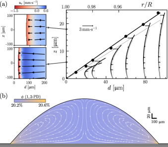
Fig. \IfSubStrfig:FIG2eq:(2)2 (a) shows the velocity field inside the droplet, as determined by PIV. The arrows indicate the velocities that have been measured in different -planes. The insets show dense velocity fields for two exemplary -planes. Close to the free surface, the flow is directed inward, precisely balanced by an outward flow close to the substrate, leading to a quasi-stationary shape.
The surface tension gradient can be derived from the tangential stress boundary condition, using the measured shear rate and the viscosity from the literature [50, 51, 52]. Fig. \IfSubStrfig:FIG3eq:(3)3 shows the experimentally derived surface tension gradient as a function of the distance to the contact line, for various diols, compositions, and relative humidities. All curves follow a power law . Despite significant differences in composition, surface activity, and ambient humidities, the curves nearly collapse in physical units.

Lubrication theory
We consider the general case of a thin liquid film of a mixture on a flat solid surface. The film covers the entire substrate, with a continuous transition between the macroscopic droplet and a microscopically thin precursor surrounding it. The latter reflects the adsorption equilibrium of vapor molecules in the atmosphere around the droplet [53]. For water above the dew point, adsorption layers on hydrophilic surfaces are typically on the order of a few [54, 55]. The free surface is described by , where is the location in the substrate plane (see Fig. \IfSubStrfig:FIG1eq:(1)1 (a)). Incompressible Stokes flow without body forces is governed by
| (1) | ||||
| (2) |
where is the fluid velocity, is the dynamic viscosity of the fluid, and is the fluid pressure. The evolution of the solute field is given by
| (3) |
with as time and as the diffusion coefficient of the solute. For simplicity we limit the following analysis to isothermal, isochoric, and isoviscous cases. We consider a no-slip and no-flux boundary condition at , kinematic and stress boundary conditions at , and a Stefan-type boundary condition that links composition and evaporation (see Supplemental Material for details [47]).
To derive evolution equations in terms of vertically averaged quantities, we take the limit of long waves, where the characteristic horizontal scale, , shall be much larger than the characteristic vertical scale, : . For sessile droplets, and are conveniently chosen as the footprint radius and the apical height of the droplet, respectively. We define the vertically averaged velocity , the total hydrodynamic flux , the vertically averaged composition , and the effective solute height through
| (4) |
and the deviations from the average by
| (5) |
We scale all horizontal coordinates as , and all vertical coordinates as . Velocities and time are scaled with and , the characteristic velocity and time scales of the problem, respectively. Below, and will be identified with the natural scales that arise in the evolution equations. Surface tension is scaled as , where , the surface tension of the pure solvent. Diffusivity is treated similarly, with . We scale for the evaporation rate, where and are determined according to Ref. [53] for the diffusion limited regime.
Whether , the vertically averaged composition, is sufficient to describe the compositional evolution of the film, depends on the magnitude of the residual field . Thus we scale , deriving from the governing equation for . In the following we will omit the primes for readability and work exclusively with scaled quantities.
The derivation of the evolution equation for the film height follows the standard procedure described in the reviews [23, 35]. One obtains
| (6) |
from integrating \IfSubStreq:ucontinuityeq:(2)2 along , where . Note that \IfSubStreq:hevoleq:(6)6 does not involve any approximation. The long wave expansion is used only in the expressions for the evaporation rate (see Ref. [53]) and the horizontal hydrodynamic flux [56]
| (7) |
Here we identified the natural velocity scale , the capillary velocity for thin films, to cancel the material properties from Eq. \IfSubStreq:Phieq:(7)7. For a typical 1,2-propanediol/water droplet with (i.e., and [57]), , and one obtains , much larger than the maximum experimentally observed velocities . This is a common observation in wetting problems, where the capillary number typically remains small. The natural pressure- and time scales are and , respectively. The pressure contains capillary and surface (disjoining) forces that stabilize the precursor film.
The capillary- () and Marangoni () fluxes are associated with Poiseuille- and Couette-type velocity profiles, respectively [47]. These will shear any horizontal compositional gradient, such that a vertical gradient arises naturally. Combined with molecular diffusion from Eq. \IfSubStreq:phicontinuityeq:(3)3, this leads to Taylor-Aris dispersion [43, 44]. In addition, the Stefan boundary condition for evaporation at the free surface requires a vertical compositional gradient [58, 59]. It is commonly accepted that vertical compositional gradients are beyond the limit of the lubrication expansion [56, 60, 61, 62, 63, 64, 38, 37]. We challenge this paradigm, identifying three regimes, depending on aspect ratio and Péclet number: i. A regime of faint vertical compositional gradients where previous long-wave models hold [56]; ii. An intermediate regime of small but not negligible vertical gradients for which we derive a previously unknown evolution equation for including Taylor-Aris dispersion; and iii. A regime of large vertical gradients where the full advection-diffusion problem has to be solved [56].
Inserting \IfSubStreq:phispliteq:(5)5 into \IfSubStreq:phicontinuityeq:(3)3 and integrating over the film height gives
| (8) |
where is the Péclet number and is the vertically averaged diffusion coefficient (see Supplemental Material [47] for a detailed derivation). In contrast to Eq. \IfSubStreq:hevoleq:(6)6, terms with non-averaged quantities remain. These terms scale as , while the next-order terms in \IfSubStreq:hevoleq:(6)6 with \IfSubStreq:Phieq:(7)7 scale as . Thus, the magnitude of relative to determines which terms in \IfSubStreq:phisplitinteq:(8)8 should be kept.
Limit i: . We may ignore all terms and recover the previously known evolution equation [56, 65, 66]:
| (9) |
Limit iii: . No simplified evolution equation for vertically averaged quantities can be derived, and the full problem has to be solved [56, 66].
Limit ii: . In this case, terms up to have to be retained. We consider a convection dominated problem i.e., and . Far below the boiling point, and with typical and , this holds for most sessile nano- to microliter droplets with small contact angles. Eq. \IfSubStreq:phisplitinteq:(8)8 simplifies further [47]:
| (10) |
The remaining term with scales as . Thus a governing equation for can be truncated to . Inserting \IfSubStreq:phispliteq:(5)5 into \IfSubStreq:phicontinuityeq:(3)3, multiplying with , and subtracting \IfSubStreq:phisplitintsimpeq:(10)10 gives the leading order governing equation for [47]:
| (11) |
where we recover the natural scale of the residual field, [65, 66]. is equivalent to a Péclet number for the characteristic vertical length- and velocity scales, and , respectively. Eq. \IfSubStreq:deltaphigoveq:(11)11 defines the advection-diffusion problem of the residual field in the co-moving frame of the mean flow: Diffusion along balances the shearing due to the horizontal flow, and the residual field is stationary at leading order.
The requirements for limit ii became apparent now: The problem must be convection dominated in the horizontal direction (), but diffusion dominated in the vertical direction, i.e., the residual field must remain small: . This is similar to the classical treatment of pipe flow by Taylor and Aris [43, 44], but here the velocity field and the film height, and thus vary in space. By scaling in Eq. \IfSubStreq:deltaphigoveq:(11)11 with the local film height , it becomes apparent that if shear () dominates. For Marangoni-contracted droplets, we find everywhere: and , which are caused by evaporative enrichment and Marangoni convection, are strong only near the edge of the droplet where the height is small (see below for a quantitative estimate).
Eq. \IfSubStreq:deltaphigoveq:(11)11 can be integrated, and the resulting expressions for and the integral in \IfSubStreq:phisplitintsimpeq:(10)10 can be found in the Supplemental Material [47]. In cases of axial or translational symmetry and slow evaporation (), which holds for our experiments, Eq. \IfSubStreq:phisplitintsimpeq:(10)10 reduces to Eq. \IfSubStreq:phiavevol:limIeq:(9)9 with replaced by to account for Taylor-Aris dispersion:
| (12) |
Numerical simulations
We implemented the evolution equations \IfSubStreq:hevoleq:(6)6 and \IfSubStreq:phiavevol:limIeq:(9)9 with the flux \IfSubStreq:Phieq:(7)7 and the effective diffusivity \IfSubStreq:Deffeq:(12)12 in an axisymmetric finite volume scheme with convergent numerical mobilities after Refs. [67, 68], and diffusion limited evaporation according to Refs. [53, 13]. We used accurate material properties , , found in the literature [50, 51, 52, 57], and assumed in accordance with the Stokes-Einstein relation. Simulations were initiated with a droplet of volume and apparent contact angle, on top of a precursor in equilibrium with the vapor field of the droplet. See [47] for details.
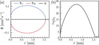
Fig. \IfSubStrfig:FIG1eq:(1)1 (d) compares the apparent contact angle observed in simulations with (dashed) and without (dash-dotted) Taylor-Aris dispersion. A near-quantitative agreement is observed for stationary contraction only if dispersion is taken into account. The remaining quantitative deviation is much smaller than the mismatch for simulations without dispersion and can be attributed to uncertainties in the material parameters, most importantly, the molecular diffusivity. We deliberately refrain from any parameter fittings. Fig. \IfSubStrfig:FIG2eq:(2)2 (b) shows stream lines and composition for a contracted droplet. The observed difference in composition between the center and edge is merely . The most striking feature of the simulations is a quantitative reproduction of the experimentally observed velocities (Fig. \IfSubStrfig:FIG2eq:(2)2 a, gray, simulation, vs. black, experiments) and surface tension gradients (Fig. \IfSubStrfig:FIG3eq:(3)3) for the case with Taylor-Aris dispersion.
The origin and importance of Taylor-Aris dispersion are highlighted in Fig. \IfSubStrfig:FIG4eq:(4)4. Panel (a) shows the strong but compensating capillary and Marangoni fluxes in the droplet. Although the net hydrodynamic flux vanishes, the different velocity profiles of capillary and Marangoni fluxes lead to a convection roll inside the droplet, and thus strong shear dispersion. This leads to an effective diffusivity (including shear dispersion and molecular diffusion, Fig. \IfSubStrfig:FIG4eq:(4)4 (b)) which scales quadratically with the individual flux components (Eq. \IfSubStreq:Deffeq:(12)12), meaning strong dispersion in regions where the fluxes are large. Here, the effective diffusivity reaches around . Thus, Taylor-Aris dispersion becomes the governing phenomenon for the solute distribution in Marangoni-contracted droplets.
Inserting again our characteristic quantities (, , , , and ), we obtain and . Thus the applicability of Taylor dispersion for our droplets depends on the magnitude of the scaled . The largest measured velocities were , close to the contact line where the scaled height (see Fig. \IfSubStrfig:FIG2eq:(2)2). The gradient of the mean composition in that region can be estimated from Fig. \IfSubStrfig:FIG3eq:(3)3 as . Thus, the deviation from the mean composition is only , which justifies the approximations.
Conclusion
We measured the internal flow fields of Marangoni-contracted drops and derived the surface tension gradient, which follows a power law . Through a systematic long wave expansion for free-surface films of mixtures, we could extend the widely used thin-film evolution equations to the case of bulk mixtures subject to Taylor-Aris dispersion. For Marangoni-contracted drops, Taylor-Aris dispersion governs the composition, and our model is in quantitative agreement with the experimental findings. The theoretical analysis enables lubrication theory to be used for the very general case of advection-dominated thin free-surface films with advected bulk fields like temperature or composition.
Note added. Recently, we became aware of another study that includes Taylor dispersion in the description of Marangoni-contracted droplets [69].
Acknowledgements.
Acknowledgments. We acknowledge financial support from the Max Planck – University of Twente Center for Complex Fluid Dynamics. S.K. acknowledges the hospitality of the Isaac Newton Institute, Cambridge, UK, during the workshop “Complex Fluids in Evolving Domains”, and helpful discussions with Uwe Thiele. We would like to thank Debmalya Roy for assistance with the experiments.References
- Lohse and Zhang [2020] D. Lohse and X. Zhang, Physicochemical hydrodynamics of droplets out of equilibrium, Nature Reviews Physics 2, 426 (2020).
- Brutin and Starov [2018] D. Brutin and V. Starov, Recent advances in droplet wetting and evaporation, Chemical Society Reviews 47, 558 (2018).
- Snoeijer and Andreotti [2013] J. H. Snoeijer and B. Andreotti, Moving contact lines: Scales, regimes, and dynamical transitions, Annual Review of Fluid Mechanics 45, 269 (2013).
- Bonn et al. [2009] D. Bonn, J. Eggers, J. Indekeu, J. Meunier, and E. Rolley, Wetting and spreading, Rev. Mod. Phys. 81, 739 (2009).
- Smith et al. [2018] E. R. Smith, P. E. Theodorakis, R. V. Craster, and O. K. Matar, Moving contact lines: Linking molecular dynamics and continuum-scale modeling, Langmuir 34, 12501 (2018).
- Brutin et al. [2010] D. Brutin, B. Sobac, B. Loquet, and J. Sampol, Pattern formation in drying drops of blood, Journal of Fluid Mechanics 667, 85 (2010).
- Traipe-Castro et al. [2014] L. Traipe-Castro, D. Salinas-Toro, D. López, M. Zanolli, M. Srur, F. Valenzuela, A. Cáceres, H. Toledo-Araya, and R. López-Solís, Dynamics of tear fluid desiccation on a glass surface: a contribution to tear quality assessment, Biological Research 47, 10.1186/0717-6287-47-25 (2014).
- Gans and Schubert [2004] B. J. D. Gans and U. S. Schubert, Inkjet printing of well-defined polymer dots and arrays, Langmuir 20, 7789 (2004).
- Park and Moon [2006] J. Park and J. Moon, Control of colloidal particle deposit patterns within picoliter droplets ejected by ink-jet printing, Langmuir 22, 3506 (2006).
- Zenit [2019] R. Zenit, Some fluid mechanical aspects of artistic painting, Physical Review Fluids 4, 110507 (2019).
- Giorgiutti-Dauphiné and Pauchard [2016] F. Giorgiutti-Dauphiné and L. Pauchard, Painting cracks: A way to investigate the pictorial matter, Journal of Applied Physics 120, 065107 (2016).
- Cira et al. [2015] N. J. Cira, A. Benusiglio, and M. Prakash, Vapour-mediated sensing and motility in two-component droplets, Nature 519, 446 (2015).
- Karpitschka et al. [2017] S. Karpitschka, F. Liebig, and H. Riegler, Marangoni contraction of evaporating sessile droplets of binary mixtures, Langmuir 33, 4682 (2017).
- Benusiglio et al. [2018] A. Benusiglio, N. J. Cira, and M. Prakash, Two-component marangoni-contracted droplets: friction and shape, Soft Matter 14, 7724 (2018).
- Sadafi et al. [2019] H. Sadafi, S. Dehaeck, A. Rednikov, and P. Colinet, Vapor-mediated versus substrate-mediated interactions between volatile droplets, Langmuir 35, 7060 (2019).
- Malinowski et al. [2020] R. Malinowski, I. P. Parkin, and G. Volpe, Nonmonotonic contactless manipulation of binary droplets via sensing of localized vapor sources on pristine substrates, Science Advances 6, 10.1126/sciadv.aba3636 (2020).
- Williams et al. [2020] A. G. L. Williams, G. Karapetsas, D. Mamalis, K. Sefiane, O. K. Matar, and P. Valluri, Spreading and retraction dynamics of sessile evaporating droplets comprising volatile binary mixtures, Journal of Fluid Mechanics 907, 10.1017/jfm.2020.840 (2020).
- Hack et al. [2021] M. A. Hack, W. Kwieciński, O. Ramírez-Soto, T. Segers, S. Karpitschka, E. S. Kooij, and J. H. Snoeijer, Wetting of two-component drops: Marangoni contraction versus autophobing, Langmuir 37, 3605 (2021), pMID: 33734702, https://doi.org/10.1021/acs.langmuir.0c03571 .
- Shiri et al. [2021] S. Shiri, S. Sinha, D. A. Baumgartner, and N. J. Cira, Thermal marangoni flow impacts the shape of single component volatile droplets on thin, completely wetting substrates, Physical Review Letters 127, 024502 (2021).
- Darhuber and Troian [2003] A. A. Darhuber and S. M. Troian, Marangoni driven structures in thin film flows, Physics of Fluids 15, S9 (2003), https://doi.org/10.1063/1.4739213 .
- Gotkis et al. [2006] Y. Gotkis, I. Ivanov, N. Murisic, and L. Kondic, Dynamic structure formation at the fronts of volatile liquid drops, Phys. Rev. Lett. 97, 186101 (2006).
- Wodlei et al. [2018] F. Wodlei, J. Sebilleau, J. Magnaudet, and V. Pimienta, Marangoni-driven flower-like patterning of an evaporating drop spreading on a liquid substrate, Nature Communications 9, 10.1038/s41467-018-03201-3 (2018).
- Oron et al. [1997] A. Oron, S. H. Davis, and S. G. Bankoff, Long-scale evolution of thin liquid films, Reviews of Modern Physics 69, 931 (1997).
- Zhang et al. [2011] J. Zhang, A. Oron, and R. P. Behringer, Novel pattern forming states for marangoni convection in volatile binary liquids, Physics of Fluids 23, 072102 (2011).
- Christy et al. [2011] J. R. E. Christy, Y. Hamamoto, and K. Sefiane, Flow transition within an evaporating binary mixture sessile drop, Physical Review Letters 106, 205701 (2011).
- Soulie et al. [2015] V. Soulie, S. Karpitschka, F. Lequien, P. Prené, T. Zemb, H. Möhwald, and H. Riegler, The evaporation behavior of sessile droplets from aqueous saline solutions, Phys. Chem. Chem. Phys. 17, 22296 (2015).
- Marin et al. [2019] A. Marin, S. Karpitschka, D. Noguera-Marín, M. A. Cabrerizo-Vílchez, M. Rossi, C. J. Kähler, and M. A. Rodríguez Valverde, Solutal marangoni flow as the cause of ring stains from drying salty colloidal drops, Phys. Rev. Fluids 4, 041601(R) (2019).
- Rossi et al. [2019] M. Rossi, A. Marin, and C. J. Kähler, Interfacial flows in sessile evaporating droplets of mineral water, Physical Review E 100, 033103 (2019).
- Karapetsas et al. [2016] G. Karapetsas, K. C. Sahu, and O. K. Matar, Evaporation of sessile droplets laden with particles and insoluble surfactants, Langmuir 32, 6871 (2016).
- Diddens [2017] C. Diddens, Detailed finite element method modeling of evaporating multi-component droplets, Journal of Computational Physics 340, 670 (2017).
- Diddens et al. [2017] C. Diddens, H. Tan, P. Lv, M. Versluis, J. G. M. Kuerten, X. Zhang, and D. Lohse, Evaporating pure, binary and ternary droplets: thermal effects and axial symmetry breaking, Journal of Fluid Mechanics 823, 470 (2017).
- Li et al. [2019] Y. Li, C. Diddens, P. Lv, H. Wijshoff, M. Versluis, and D. Lohse, Gravitational effect in evaporating binary microdroplets, Physical Review Letters 122, 114501 (2019).
- van Gaalen et al. [2021] R. T. van Gaalen, C. Diddens, H. M. A. Wijshoff, and J. G. M. Kuerten, Marangoni circulation in evaporating droplets in the presence of soluble surfactants, Journal of Colloid and Interface Science 584, 622 (2021).
- Pahlavan et al. [2021] A. A. Pahlavan, L. Yang, C. D. Bain, and H. A. Stone, Evaporation of binary-mixture liquid droplets: The formation of picoliter pancakelike shapes, Physical Review Letters 127, 024501 (2021).
- Craster and Matar [2009] R. V. Craster and O. K. Matar, Dynamics and stability of thin liquid films, Reviews of Modern Physics 81, 1131 (2009).
- Thiele et al. [2012] U. Thiele, A. J. Archer, and M. Plapp, Thermodynamically consistent description of the hydrodynamics of free surfaces covered by insoluble surfactants of high concentration, Physics of Fluids 24, 102107 (2012).
- Thiele et al. [2016] U. Thiele, A. J. Archer, and L. M. Pismen, Gradient dynamics models for liquid films with soluble surfactant, Physical Review Fluids 1, 083903 (2016).
- Xu et al. [2015] X. Xu, U. Thiele, and T. Qian, A variational approach to thin film hydrodynamics of binary mixtures, Journal of Physics: Condensed Matter 27, 085005 (2015).
- Moshinskii [2004] A. I. Moshinskii, Equivalent diffusion in a thin film flow with a non-one-dimensional velocity field and anisotropic diffusion tensor, Fluid Dynamics 39, 230 (2004).
- Ajdari et al. [2006] A. Ajdari, N. Bontoux, and H. A. Stone, Hydrodynamic dispersion in shallow microchannels: the effect of cross-sectional shape, Analytical Chemistry 78, 387 (2006).
- Mukahal et al. [2017] F. H. H. A. Mukahal, B. R. Duffy, and S. K. Wilson, Advection and taylor–aris dispersion in rivulet flow, Proceedings of the Royal Society A: Mathematical, Physical and Engineering Sciences 473, 20170524 (2017).
- Vilquin et al. [2020] A. Vilquin, V. Bertin, P. Soulard, G. Guyard, E. Raphael, F. Restagno, T. Salez, and J. D. McGraw, Time dependence of advection-diffusion coupling for nanoparticle ensembles, Phys. Rev. Fluids 6, 064201 (2021).
- Taylor [1953] G. I. Taylor, Dispersion of soluble matter in solvent flowing slowly through a tube, Proceedings of the Royal Society of London. Series A. Mathematical and Physical Sciences 219, 186 (1953).
- Aris [1956] R. Aris, On the dispersion of a solute in a fluid flowing through a tube, Proceedings of the Royal Society of London. Series A. Mathematical and Physical Sciences 235, 67 (1956).
- Chakrabarti and Saintillan [2020] B. Chakrabarti and D. Saintillan, Shear-induced dispersion in peristaltic flow, Physics of Fluids 32, 113102 (2020).
- Darhuber et al. [2004] A. A. Darhuber, J. Z. Chen, J. M. Davis, and S. M. Troian, A study of mixing in thermocapillary flows on micropatterned surfaces, Philosophical Transactions of the Royal Society of London. Series A: Mathematical, Physical and Engineering Sciences 362, 1037 (2004).
- [47] See supplemental material at http://link.aps.org/supplemental/… for additional details about the experiments and the simulations, which includes Refs. [48, 49].
- Leonard and Mokhtari [1990] B. P. Leonard and S. Mokhtari, Beyond first-order upwinding: The ultra-sharp alternative for non-oscillatory steady-state simulation of convection, International Journal for Numerical Methods in Engineering 30, 729 (1990).
- Cohen et al. [1996] S. D. Cohen, A. C. Hindmarsh, and P. F. Dubois, CVODE, a stiff/nonstiff ODE solver in c, Computers in Physics 10, 138 (1996).
- Moosavi and Rostami [2017] M. Moosavi and A. A. Rostami, Densities, viscosities, refractive indices, and excess properties of aqueous 1,2-etanediol, 1,3-propanediol, 1,4-butanediol, and 1,5-pentanediol binary mixtures, Journal of Chemical and Engineering Data 62, 156 (2017).
- George and Sastry [2003] J. George and N. V. Sastry, Density, dynamic viscosities, speeds of sound, and relative permittivities for water + alkanediols (propane-1,2- and -1,3-diol and butane-1,2-, -1,3-, -1,4-, and -2,3-diol) at different temperatures, Journal of Chemical and Engineering Data 48, 1529 (2003).
- Jarosiewicz et al. [2004] P. Jarosiewicz, G. Czechowski, and J. Jadżyn, The viscous properties of diols. v. 1,2-hexanediol in water and butanol solutions, Verlag der Zeitschrift für Naturforschung A 59, 559 (2004).
- Eggers and Pismen [2010] J. Eggers and L. M. Pismen, Nonlocal description of evaporating drops, Physics of Fluids 22, 112101 (2010).
- Verdaguer et al. [2007] A. Verdaguer, C. Weis, G. Oncins, G. Ketteler, H. Bluhm, and M. Salmeron, Growth and structure of water on SiO2 films on si investigated by kelvin probe microscopy and in situ x-ray spectroscopies, Langmuir 23, 9699 (2007).
- Barnette et al. [2008] A. L. Barnette, D. B. Asay, and S. H. Kim, Average molecular orientations in the adsorbed water layers on silicon oxide in ambient conditions, Physical Chemistry Chemical Physics 10, 4981 (2008).
- Matar [2002] O. K. Matar, Nonlinear evolution of thin free viscous films in the presence of soluble surfactant, Physics of Fluids 14, 4216 (2002).
- Karpitschka and Riegler [2010] S. Karpitschka and H. Riegler, Quantitative experimental study on the transition between fast and delayed coalescence of sessile droplets with different but completely miscible liquids, Langmuir 26, 11823 (2010).
- Karpitschka et al. [2015] S. Karpitschka, C. Weber, and H. Riegler, Spin casting of dilute solutions: Vertical composition profile during hydrodynamic-evaporative film thinning, Chem. Eng. Sci. 129, 243 (2015).
- Hennessy et al. [2017] M. G. Hennessy, G. L. Ferretti, J. T. Cabral, and O. K. Matar, A minimal model for solvent evaporation and absorption in thin films, Journal of Colloid and Interface Science 488, 61 (2017).
- Oron and Nepomnyashchy [2004] A. Oron and A. A. Nepomnyashchy, Long-wavelength thermocapillary instability with the soret effect, Physical Review E 69, 016313 (2004).
- Shklyaev et al. [2007] S. Shklyaev, A. A. Nepomnyashchy, and A. Oron, Three-dimensional oscillatory long-wave marangoni convection in a binary liquid layer with the soret effect: Bifurcation analysis, Physics of Fluids 19, 072105 (2007).
- Shklyaev et al. [2011] S. Shklyaev, A. A. Nepomnyashchy, and A. Oron, Oscillatory long-wave marangoni convection in a layer of a binary liquid: Hexagonal patterns, Physical Review E 84, 056327 (2011).
- Thiele [2011] U. Thiele, Note on thin film equations for solutions and suspensions, The European Physical Journal Special Topics 197, 213 (2011).
- Thiele et al. [2013] U. Thiele, D. V. Todorova, and H. Lopez, Gradient dynamics description for films of mixtures and suspensions: Dewetting triggered by coupled film height and concentration fluctuations, Physical Review Letters 111, 117801 (2013).
- Jensen and Grotberg [1993] O. E. Jensen and J. B. Grotberg, The spreading of heat or soluble surfactant along a thin liquid film, Physics of Fluids A: Fluid Dynamics 5, 58 (1993).
- Jensen et al. [1994] O. E. Jensen, D. Halpern, and J. B. Grotberg, Transport of a passive solute by surfactant-driven flows, Chemical Engineering Science 49, 1107 (1994).
- Diez et al. [2000] J. A. Diez, L. Kondic, and A. Bertozzi, Global models for moving contact lines, Physical Review E 63, 011208 (2000).
- Lenz et al. [2002] M. Lenz, M. Rumpf, and G. Grün, A finite volume scheme for surfactant driven thin film flow, in Proceedings of the Third International Symposium on Finite Volumes for Complex Applications, edited by R. Herbin and D. Kröner (Hermes Penton Science, 2002) pp. 567–574.
- Charlier et al. [2022] J. Charlier, A. Rednikov, S. Dehaeck, P. Colinet, and D. Terwagne, Water-propylene glycol sessile droplet shapes and migration: Marangoni mixing and separation of scales, J. Fluid Mech. 933, A45 (2022).