Distributed Newton Optimization with Maximized Convergence Rate

Abstract

The distributed optimization problem is set up in a collection of nodes interconnected via a communication network. The goal is to find the minimizer of a global objective function formed by the addition of partial functions locally known at each node. A number of methods are available for addressing this problem, having different advantages. The goal of this work is to achieve the maximum possible convergence rate. As the first step towards this end, we propose a new method which we show converges faster than other available options. As with most distributed optimization methods, convergence rate depends on a step size parameter. As the second step towards our goal we complement the proposed method with a fully distributed method for estimating the optimal step size that maximizes convergence speed. We provide theoretical guarantees for the convergence of the resulting method in a neighborhood of the solution. Also, for the case in which the global objective function has a single local minimum, we provide a different step size selection criterion together with theoretical guarantees for convergence. We present numerical experiments showing that, when using the same step size, our method converges significantly faster than its rivals. Experiments also show that the distributed step size estimation method achieves an asymptotic convergence rate very close to the theoretical maximum.

I Introduction

A networked system is a web of intelligent sensing and computing devices connected via a communication network. Its main goal is to carry out a computational task in a distributed manner, by executing a cooperative strategy over all the nodes of the network without centralized coordination. The design of distributed algorithms is constrained by the fact that each node is limited in computational power and communication bandwidth. Distributed algorithms are available for parameter estimation [1, 2], Kalman filtering [3], control [4, 5], optimization [6], etc.

The goal of a distributed optimization method is to minimize a cost function formed by a sum of local functions which are only known by each node [7, 6, 8, 9, 10]. It finds applications in power systems, sensor networks, smart buildings, smart manufacturing, etc. The available distributed optimization methods can be classified according to different criteria. We describe below those criteria used in this work.

One classification criterion is between sequential and simultaneous methods. In a sequential method, nodes take turns to tune its local variables using its local function as well as information received from other nodes [11]. The main drawback of these methods is that they do not scale well for large networks, since many turns are needed to guarantee that all nodes are visited. Also, for a fully distributed implementation, a distributed mechanism is needed to guarantee that each node is regularly visited in the sequence. A popular approach within this line are methods based on alternating direction method of multipliers [12, 13]. In contrast to sequential methods, a simultaneous method iterates over a computation step, in which all nodes carry out local computations, and a communication step, in which nodes communicate information with their neighbors. These two steps typically depend on the number of local neighbors and not on the network size. In this way, simultaneous methods avoid the scalability problems of sequential ones.

Another classification criterion is between methods using first order derivatives and those using derivatives of second order. There is a vast literature on first order methods [14, 15, 16, 17, 18, 19] as well as the survey [6]. As with centralized optimization methods, the advantage of first order distributed methods is that they are simpler to implement and analyze. However, second order distributed methods converge much faster, leading to less computational and communication requirements.

Upon convergence, a distributed optimization method needs to guarantee that all nodes obtain the same optimal value. Another classification criterion is based on how the distributed method guarantees this inter-node matching property. One approach consists in adding a constraint to the optimization program forcing this property. In [20, 21] the resulting constrained optimization problem is solved by adding a penalization term. This gives an approximate solution which becomes exact as the step size used in the optimization recursions decreases to zero. This has the disadvantage of slowing down convergence. This is avoided in [22] by solving the constrained optimization program via its dual. However, at each iteration each node needs to solve a local optimization problem needed to evaluate the Lagrange dual function. These two approaches were also considered in [23]. All these methods require the local functions at each node to be strongly convex, which is a somehow strong requirement, since these local functions typically represent partial information about the variables to be optimized. They also require, at each iteration, inverting a matrix using a recursive inversion formula. This requires running sub-iterations, each involving a computation/communication step, between every two main iterations. These drawbacks are avoided by forcing the inter-node matching using average consensus. By doing so the resulting optimization program is unconstrained. As pointed out in [24], an additional advantage of this approach is that the large literature available for average consensus permits guaranteeing its robustness to asynchronous communications, packet losses, time-varying network topology, undirected communication links, etc.

In view of the above classification, we are interested in simultaneous second order distributed methods based on average consensus. A seminal method within this line was introduced in [24, 25]. It was then extended in [26] to deal with asynchronous communications, in [27] to deal with lossy communications, and in [28] to deal with event-triggered communications in the context of continuous-time optimization methods. A fast convergent variant of this method was proposed in [29] using finite-time average consensus. However, this kind of consensus requires global knowledge of the network structure, hence the method is not fully distributed. In this work we build upon this line by focusing on convergence speed. Our contributions are the following: (1) We propose a variant of the aforementioned distributed method. The proposed variant converges much faster than the other methods, for the same optimization step size. Moreover, it is also more robust to the choice of the step size, in the sense that it converges with step sizes which are large enough to cause the divergence of other methods. This permits choosing larger step sizes to speed up convergence. (2) We propose a fully distributed method for determining, at each node, the optimal step size in the sense of maximizing the asymptotic convergence speed. We also do a theoretical convergence analysis guaranteeing the convergence of the resulting distributed optimization procedure, when used in conjunction with the proposed step size selection algorithm, in a neighborhood of the solution. (3) In the case in which the global objective function has a single local minimum, we provide a different step size selection criterion, together with sufficient conditions to guarantee the global convergence of the proposed algorithm. This result is stronger than most available ones in the sense that we require that the global objective function, rather than each local function, is strongly convex.

The rest of the paper is organized as follows. In Section II we state the research problem. In Section III we derive the proposed distributed optimization method and compare it with other available methods. In Section IV we describe the proposed distributed method for step size selection. In Section V we do the global convergence analysis in the case of a single local minimum. In Section VI we apply our results to a practical problem, namely, target localization, and present numerical experiments confirming our claims. Concluding remarks are given in Section VII.

II Problem statement

Notation 1.

The set of natural and real numbers are denoted by $\mathbb{N}$ and $\mathbb{R}$, respectively. For a vector $x\in\mathbb{R}^{N}$, we use $\left\|x\right\|$ to denote its $2$-norm and $\left\|x\right\|_{P}=\sqrt{x^{\top}Px}$ to denote its $P>0$ weighted 2-norm. For a matrix $A\in\mathbb{R}^{N\times N}$, we use $\left\|A\right\|_{\mathrm{F}}$ to denote its Frobenius norm, $\left\|A\right\|$ to denote its operator norm (induced by the vector $2$-norm) and $\rho(A)$ its spectral radius. Also, $\mathbf{I}_{N}$ denotes the $N\times N$ identity matrix and $\mathbf{1}_{N}$ the $N$-dimensional column vector filled with ones. To simplify the notation we often omit the subscript in $\mathbf{I}_{N}$ and $\mathbf{1}_{N}$ when the dimension can be clearly inferred from the context. We use $\mathrm{col}\left(x_{1},\cdots,x_{I}\right)$ to denote the column vector formed by stacking the elements $x_{1},\cdots,x_{I}$ and $\otimes$ to denote the Kronecker product. We use $\leq$ to denote the non-strict partial order on $\mathbb{R}^{N}$ defined by $x\leq y$ if $x_{i}\leq y_{i}$, for all $i=1,\cdots,I$, and $<$ to denote the strict partial order corresponding to $\leq$, i.e., $x<y$ if $x\leq y$ and $x\neq y$. Finally, $O(x)$ denotes Bachmann–Landau’s big O notation $O(x)$ as $x\rightarrow 0$.

We have a network of $I$ nodes. Node $i$ can evaluate the function $f^{i}:\mathbb{R}^{N}\rightarrow\mathbb{R}$ and send messages to its out-neighbors $\mathcal{N}_{i}\subseteq\{1,\cdots,I\}$ using a consensus network. The communication link from node $i$ to node $j\in\mathcal{N}_{i}$ has time-invariant gain $w^{j,i}$. We assume that $w^{i,j}=0$ if $j\neq\mathcal{N}_{i}$. We also assume that the graph induced by the communication network is balanced (i.e., possibly directed) and strongly connected. This implies that matrix $W=\left[w^{i,j}\right]_{i,j=1}^{I}$ is doubly stochastic and primitive. As explained in [30], a consequence of this is that $\mathbf{1}_{I}^{\top}W=\mathbf{1}_{I}^{\top}$ and $W\mathbf{1}_{I}=\mathbf{1}_{I}$. Also, for any $x_{1}=\left[x_{1}^{i},\cdots,x_{1}^{I}\right]^{\top}\in\mathbb{R}^{I}$, the sequence generated by $x_{k+1}=Wx_{k}$ satisfies

$$\lim_{k\rightarrow\infty}x_{k}=\mathbf{1}_{I}\otimes\frac{1}{I}\sum_{i=1}^{I}x_{1}^{i}.$$

The goal of distributed optimization is to design a distributed method for solving the following minimization problem

$$x_{\star}\in\underset{x\in\mathbb{R}^{N}}{\arg\min}f(x)\quad\text{with}\quad f(x)=\frac{1}{I}\sum_{i=1}^{I}f^{i}(x).$$ (1)

Solving (1) using a centralized or distributed method requires certain assumptions on the objective function $f$, e.g., convexity, quasi-convexity, everywhere positive definite Hessian matrix, etc. These assumptions may be too strong in certain applications. When none of these assumptions can be made, it is often enough to solve

$$x_{\star}\in\underset{x\in\mathbb{R}^{N}}{\mathrm{loc\,min}}f(x),$$ (2)

where $\mathrm{loc\,min}$ denotes the set of local minimizers of $f$.

As mentioned in the introduction, a number of methods are available for solving either (1) or (2), and our preferred choice is the family of methods in [24, 25, 26, 27, 28]. In Section III we derive a new method that can be regarded as a variant of the aforementioned ones. As we explain, its design aims at maximizing convergence speed. In Section IV we focus on the general problem (2) in which convergence to the global optimum cannot be guaranteed. We propose a step size selection criterion to maximize local convergence speed. In Section V we focus on (1) and provide a selection criterion to guarantee convergence to the global optimum, in the case where the global function $f$ is strongly convex.

III Proposed method

In this section we introduce the proposed distributed optimization method with fixed step size. In Section III-A we introduce some background on static and dynamic average consensus. Using this, in Section III we derive the proposed method, and in Section III-C describe its differences with respect to the variant that has been used in the literature. In Section III-D we derive two state-space representations of the algorithm which are instrumental for our convergence studies.

III-A Static and dynamic average consensus

As described in Section I, we are interested in methods achieving inter-node matching of minimization parameters via average consensus. In this section we briefly describe the options available for doing so.

Suppose that, in the network described in Section II, each node $i$ knows a variable $v^{i}\in\mathbb{V}$, $i\in\mathbb{N}$, where $\mathbb{V}$ is a vector space. In order to make the presentation valid in the general case, we assume that $\mathbb{V}$ is an arbitrary vector space, i.e., each $v^{i}$ can be either a scalar, a vector, a matrix, etc. The goal of (static) average consensus is to compute the average $u=\frac{1}{I}\sum_{i=1}^{I}v^{i}$ in a distributed manner. This is done using the following iterations

$$v_{k+1}^{i}=\sum_{j=1}^{I}w^{i,j}v_{k}^{j},$$

initialized by $v_{1}^{i}=v^{i}$ [30]. Letting $\mathbf{v}_{k}=\mathrm{col}\left(v_{k}^{1},\cdots,v_{k}^{I}\right)\in\mathbb{V}^{I}$ we can write the above compactly as follows

$$\mathbf{v}_{k+1}=W\mathbf{v}_{k}.$$ (3)

Suppose now that each node $i$ knows a time-varying sequence of variables $v_{k}^{i}\in\mathbb{V}$, $k\in\mathbb{N}$. The goal of the dynamic average consensus technique [31] is to obtain, at each $k$, an estimate of the average $u_{k}=\frac{1}{I}\sum_{i=1}^{I}v_{k}^{i}$. This is done as follows: Suppose that at time $k$ node $i$ knows an estimate $u_{k-1}^{i}$ of $u_{k-1}$. It then transmits the following message

$$s_{k}^{i}=u_{k-1}^{i}+v_{k}^{i}-v_{k-1}^{i},$$ (4)

to its out-neighbors. On reception, node $i$ obtains

$$u_{k}^{i}=\sum_{j=1}^{I}w^{i,j}s_{k}^{j}.$$ (5)

The above iterations are initialized by $s_{1}^{i}=v_{1}^{i}$. We can combine (4)-(5) in two ways, namely, in message form

$$s_{k+1}^{i}=\sum_{j=1}^{I}w^{i,j}s_{k}^{j}+v_{k+1}^{i}-v_{k}^{i},$$

or in estimate form

$$u_{k+1}^{i}=\sum_{j=1}^{I}w^{i,j}\left(u_{k}^{j}+v_{k+1}^{j}-v_{k}^{j}\right).$$

III-B The proposed method

The essential idea consists in distributing the Newton iterations

$$x_{k+1}=x_{k}-\alpha_{k}\left[\nabla^{2}f\left(x_{k}\right)\right]^{-1}\nabla f\left(x_{k}\right),$$ (6)

where $\alpha_{k}$ is called the step size at time $k$. To this end we make use of the dynamic average consensus technique [31]. Let

$$\bar{f}\left(x_{k}^{1},\cdots,x_{k}^{I}\right)=\frac{1}{I}\sum_{i=1}^{I}f^{i}\left(x_{k}^{i}\right).$$

We can obtain an estimate $g_{k}^{i}$ of $\nabla\bar{f}\left(x_{k}^{1},\cdots,x_{k}^{I}\right)=\frac{1}{I}\sum_{i=1}^{I}\nabla f^{i}\left(x_{k}^{i}\right)$, at each node $i$, by applying dynamic average consensus on the inputs $\nabla f^{i}\left(x_{k}^{i}\right)$. This yields the following recursions written in estimate form

$$g_{k}^{i}=\sum_{j=1}^{I}w^{i,j}\left[g_{k-1}^{j}+\nabla f^{j}\left(x_{k}^{j}\right)-\nabla f^{j}\left(x_{k-1}^{j}\right)\right].$$

We can do the same to obtain an estimate $H_{k}^{i}$ of the Hessian $\nabla^{2}\bar{f}\left(x_{k}^{1},\cdots,x_{k}^{I}\right)=\frac{1}{I}\sum_{i=1}^{I}\nabla^{2}f^{i}\left(x_{k}^{i}\right)$ using the inputs $\nabla^{2}f^{i}\left(x_{k}^{i}\right)$. This gives

$$H_{k}^{i}=\sum_{j=1}^{I}w^{i,j}\left[H_{k-1}^{j}+\nabla^{2}f^{j}\left(x_{k}^{j}\right)-\nabla^{2}f^{j}\left(x_{k-1}^{j}\right)\right].$$

It is easy to see that $\bar{f}\left(x,\cdots,x\right)=f(x)$. Hence, if

$$x_{k}^{i}\simeq x_{k}\quad\text{for all}\quad i\in\{1,\cdots,I\},$$ (7)

and some $x_{k}$, then $g_{k}^{i}$ and $H_{k}^{i}$ are estimates of $\nabla f\left(x_{k}\right)$ and $\nabla^{2}f\left(x_{k}\right)$, respectively. Thus, in principle, each node $i$ could use $g_{k}^{i}$ and $H_{k}^{i}$, in place of $\nabla f\left(x_{k}\right)$ and $\nabla^{2}f\left(x_{k}\right)$ to locally carry out the iterations (6). This would yield, at node $i$, the following sequence of estimates of $x_{\star}$

$$\breve{x}_{k+1}^{i}=\breve{x}_{k}^{i}-\alpha_{k}^{i}\left[H_{k}^{i}\right]^{-1}g_{k}^{i}.$$

But the above requires (7) to hold, with $x_{k}^{i}$ replaced by $\breve{x}_{k}^{i}$. In order to enforce that, once again we apply dynamic average consensus on the inputs $\breve{x}_{k}^{i}$. Writing the result in message form we obtain

$$x_{k+1}=\sum_{j=1}^{I}w^{i,j}x_{k}^{j}+\breve{x}_{k+1}^{i}-\breve{x}_{k}^{i}=\sum_{j=1}^{I}w^{i,j}x_{k}^{j}-\alpha_{k}^{i}\left[H_{k}^{i}\right]^{-1}g_{k}^{i}.$$

Finally, since the approximations $H_{k}^{i}$ to the Hessian are obtained via dynamic average consensus on the local Hessian matrices $\nabla f^{j}\left(x_{k}^{j}\right)$, and the latter may fail to be positive definite, some mechanism is required to guarantee that $H_{k}^{i}$ is positive definite. To do so we let $\beta>0$ and use a map $B:$ to guarantee that $B\left(H_{k}^{i}\right)\geq\beta^{-1}\mathbf{I}$. The map $B$ is defined as follows: Let $H\in\mathbb{R}^{N}$ be symmetric and $H=U\Lambda U^{\top}$ be its spectral decomposition, with $\Lambda=\mathrm{diag}\left(\lambda_{1},\cdots,\lambda_{N}\right)$. Let $\tilde{\Lambda}=\mathrm{diag}\left(\tilde{\lambda}_{1},\cdots,\tilde{\lambda}_{N}\right)$ with $\tilde{\lambda}_{i}=\lambda_{i}$ if $\lambda_{i}\geq\beta^{-1}$ and $\tilde{\lambda}_{i}=\beta^{-1}$ otherwise. Then

$$B(H)=U\tilde{\Lambda}U^{\top}.$$

The question then arises as to how to choose the parameter $\beta$. This is given in Assumptions 1 and 2 of our main results given in Sections IV and V, respectively.

To summarize the above, the proposed algorithm is given by the following recursions,

$$x_{k+1}^{i} =\sum_{j=1}^{I}w^{i,j}x_{k}^{j}-\alpha_{k}^{i}B\left(H_{k}^{i}\right)^{-1}g_{k}^{i},$$ (8)

$$g_{k+1}^{i} =\sum_{j=1}^{I}w^{i,j}\left[g_{k}^{j}+\nabla f^{j}\left(x_{k+1}^{j}\right)-\nabla f^{j}\left(x_{k}^{j}\right)\right],$$ (9)

$$H_{k+1}^{i} =\sum_{j=1}^{I}w^{i,j}\left[H_{k}^{j}+\nabla^{2}f^{j}\left(x_{k+1}^{j}\right)-\nabla^{2}f^{j}\left(x_{k}^{j}\right)\right].$$ (10)

which are initialized by

$$x_{1}^{i}=x_{\mathrm{init}}^{i},\quad g_{1}^{i}=\nabla f^{i}\left(x_{\mathrm{init}}^{i}\right)\quad\text{and}\quad H_{1}^{i}=\nabla^{2}f^{i}\left(x_{\mathrm{init}}^{i}\right).$$ (11)

Remark 1.

The reader may wonder why we choose to write (8) in message form while (9) and (10) in estimate form. This is done to put the algorithm in a form compatible with other algorithms in the literature.

Remark 2.

Notice that the information exchanged by each node at each time step does not grow with the network size, as it depends on the number of out neighbors of each node. This property is common to all simultaneous, second order methods based on average consensus [24, 25, 26, 27, 28].

III-C Comparison with similar algorithms

As mentioned above, the proposed algorithm (8)-(10) is a variant of the algorithm used in [24, 25, 26, 27, 28]. The latter differ from (8)-(10) in essentially two aspects. The first one is that consensus is not done on the parameters $x_{k}^{i}$. This means that (8) is replaced by

$$x_{k+1}^{i} =x_{k}^{i}-\alpha_{k}^{i}B\left(H_{k}^{i}\right)^{-1}g_{k}^{i}.$$ (12)

Together with (9)-(10), equation (12) forms an algorithm that, for latter reference, we refer to as Algorithm A.

The second difference consists in using the following transformation of (6)

$$x_{k+1}=(1-\alpha)x_{k}+\alpha_{k}^{i}\left(\nabla^{2}f\left(x_{k}\right)\right)^{-1}\ell\left(x_{k}\right),$$ (13)

where $\ell(x)=\nabla^{2}f(x)x-\nabla f(x)$. Using dynamic average consensus, we can estimate $\ell\left(x_{k}\right)$ at each node using

$$l_{k+1}^{i}=\sum_{j=1}^{I}w^{i,j}\left[l_{k}^{j}+\ell^{j}\left(x_{k+1}^{j}\right)-\ell^{j}\left(x_{k}^{j}\right)\right],$$ (14)

where $\ell^{i}(x)=\nabla^{2}f^{i}(x)x-\nabla f^{i}(x)$. We can then distribute iterations (13) as follows

$$x_{k+1}^{i} =\left(1-\alpha_{k}^{i}\right)\sum_{j=1}^{I}w^{i,j}x_{k}^{j}+\alpha_{k}^{i}B\left(H_{k}^{i}\right)^{-1}l_{k}^{i}.$$ (15)

We refer to the algorithm resulting from (15), (14) and (10) as Algorithm B.

Finally, the algorithm used in [24, 25, 26, 27, 28], apart from other minor differences, essentially consists in combining the modifications introduced by Algorithms A and B. This leads to the recursions formed by

$$x_{k+1}^{i}=\left(1-\alpha_{k}^{i}\right)x_{k}^{i}+\alpha_{k}^{i}B\left(H_{k}^{i}\right)^{-1}l_{k}^{i},$$ (16)

together with (10) and (14). We refer to it as Algorithm VZCPS, standing for the initials of the authors which proposed it.

As we show with experiments in Section VI, the modifications (12) and (14)-(15), introduced by Algorithms A and B, respectively, drastically slow down convergence and can cause instability. More precisely, (12) does not guarantee the convergence of each $x_{k}^{i}$ to $x_{\star}$, due to the lack of consensus on these parameters. Convergence only occurs if modification (14)-(15) is also considered, i.e., in the VZCPS algorithm, although at a much slower rate. However, a feature of the latter modification is that the first term in (15) pushes the local variables $x_{k}^{i}$ towards zero at each iteration. This pushing is compensated by the second term, but only after consensus on the parameters $x_{k}^{i}$ is reached. Before this happens, this zero pushing effect has a negative influence if the minimizing parameters $x_{\star}$ are far from zero. As we show in Section VI, this can slow down convergence and even cause instability.

III-D State-space representation

We introduce the following required notation.

Notation 2.

Let $A=\frac{1}{I}\mathbf{1}_{I}\mathbf{1}_{I}^{\top}$, $\mathbf{A}\mathbf{=}A\otimes\mathbf{I}_{N}$, $\mathbf{a}=\frac{1}{I}\mathbf{1}_{I}\otimes\mathbf{I}_{N}$ and $\tilde{\mathbf{I}}\mathbf{=}\mathbf{I}-\mathbf{A}$. Let also $\mathbf{x}_{\star}=\mathbf{1}_{I}\otimes x_{\star}$, $\mathbf{x}_{k}=\mathrm{col}\left(x_{k}^{1},\cdots,x_{k}^{I}\right)$, $\bar{\mathbf{x}}_{k}=\mathbf{A}\mathbf{x}_{k}$ and $\tilde{\mathbf{x}}_{k}=\mathbf{x}_{k}-\bar{\mathbf{x}}_{k}$. We similarly define $\mathbf{g}_{k}=\mathrm{col}\left(g_{k}^{1},\cdots,g_{k}^{I}\right)$, $\bar{\mathbf{g}}_{k}=\mathbf{A}\mathbf{g}_{k}$ and $\tilde{\mathbf{g}}_{k}=\mathbf{g}_{k}-\bar{\mathbf{g}}_{k}$ as well as $\mathbf{h}_{k}=\mathrm{col}\left(H_{k}^{1},\cdots,H_{k}^{I}\right)$, $\bar{\mathbf{h}}_{k}=\mathbf{A}\mathbf{h}_{k}$, $\tilde{\mathbf{h}}_{k}=\mathbf{h}_{k}-\bar{\mathbf{h}}_{k}$, $\mathbf{h}_{\star}=\mathbf{1}_{I}\otimes\nabla^{2}f\left(x_{\star}\right)$ and $\mathbf{H}_{\star}=\mathbf{I}_{I}\otimes\nabla^{2}f\left(x_{\star}\right)$. Finally, $\boldsymbol{\alpha}_{k}=\mathrm{diag}\left(\alpha_{k}^{1},\cdots,\alpha_{k}^{I}\right)\otimes\mathbf{I}_{I}$.

Remark 3.

In the above notation, $\bar{\mathbf{x}}_{k}$ is a block vector with all its sub-vectors equal to the average

$$\bar{x}_{k}=\frac{1}{I}\sum_{i=1}^{I}x_{k}^{i}.$$ (17)

Also, $\tilde{\mathbf{x}}_{k}$ is a block vector whose $i$-th sub-vector is given by $\tilde{x}_{k}^{i}=x_{k}^{i}-\bar{x}_{k}$. Finally, notice that $\mathbf{h}_{k}$ is a (column) vector of matrices, i.e., $\mathbf{h}_{k}\in\mathbb{R}^{IN\times N}$.

Notation 3.

For a block vector $\mathbf{x}=\mathrm{col}\left(x^{1},\cdots,x^{I}\right),$let

$$\mathfrak{g}\left(\mathbf{x}\right) =\mathrm{col}\left(\nabla f^{1}\left(x^{1}\right),\cdots,\nabla f^{I}\left(x^{I}\right)\right),$$

$$\mathfrak{h}\left(\mathbf{x}\right) =\mathrm{col}\left(\nabla^{2}f^{1}\left(x^{1}\right),\cdots,\nabla^{2}f^{I}\left(x^{I}\right)\right),$$

$$\mathfrak{H}\left(\mathbf{x}\right) =\mathrm{diag}\left(\mathfrak{h}\left(\mathbf{x}\right)\right),$$

and for a block diagonal matrix $\mathbf{H}=\mathrm{diag}\left(H^{1},\dots.H^{I}\right)$, let

$$\mathfrak{B}\left(\mathbf{H}\right)=\mathrm{diag}\left(B\left(H^{1}\right),\cdots,B\left(H^{I}\right)\right).$$

Let also $\mathbf{H}_{k}=\mathrm{diag}\left(\mathbf{h}_{k}\right)$ and $\mathbf{B}_{k}=\mathfrak{B}\left(\mathbf{H}_{k}\right)$. Let finally $W=\left[w^{i,j}\right]_{i,j=1}^{I}$ and $\mathbf{W}=W\otimes\mathbf{I}_{N}$.

Using the above notation we can write (8)-(10) in the following block state-space form

$$\mathbf{x}_{k+1} =\mathbf{W}\mathbf{x}_{k}-\boldsymbol{\alpha}_{k}\mathbf{B}_{k}^{-1}\mathbf{g}_{k},$$ (18)

$$\mathbf{g}_{k+1} =\mathbf{W}\left[\mathbf{g}_{k}+\mathfrak{g}\left(\mathbf{x}_{k+1}\right)-\mathfrak{g}\left(\mathbf{x}_{k}\right)\right],$$ (19)

$$\mathbf{h}_{k+1} =\mathbf{W}\left[\mathbf{h}_{k}+\mathfrak{h}\left(\mathbf{x}_{k+1}\right)-\mathfrak{h}\left(\mathbf{x}_{k}\right)\right].$$ (20)

A problem of the above model for studying stability is that $\rho\left(\mathbf{W}\right)=1$. Our next step is to transform (18)-(20) into an equivalent model which avoids this drawback.

Notation 4.

Let $\bar{\mathfrak{g}}\left(\mathbf{x}\right)=\mathbf{A}\mathfrak{g}\left(\mathbf{x}\right)$ and $\bar{\mathfrak{h}}\left(\mathbf{x}\right)=\mathbf{A}\mathfrak{h}\left(\mathbf{x}\right)$. Let also $\bar{\mathfrak{H}}\left(\mathbf{x}\right)=\mathrm{diag}\left(\bar{\mathfrak{h}}\left(\mathbf{x}\right)\right)$, $\bar{\mathbf{H}}_{k}=\mathrm{diag}\left(\bar{\mathbf{h}}_{k}\right)$, $\tilde{\mathbf{H}}_{k}=\mathrm{diag}\left(\tilde{\mathbf{h}}_{k}\right)$ and $\tilde{\mathbf{W}}=\mathbf{W}-\mathbf{A}$.

Lemma 1.

The following equivalences hold

$$\bar{\mathbf{g}}_{k}=\bar{\mathfrak{g}}\left(\mathbf{x}_{k}\right),\qquad\bar{\mathbf{h}}_{k}=\bar{\mathfrak{h}}\left(\mathbf{x}_{k}\right),\qquad\bar{\mathbf{H}}_{k}=\bar{\mathfrak{H}}\left(\mathbf{x}_{k}\right).$$ (21)

Proof:

Since matrix $W$ is doubly stochastic, it follows that $\mathbf{A}\mathbf{W}=\mathbf{A}$. Then, from (19)

$$\bar{\mathbf{g}}_{k+1}=\mathbf{A}\mathbf{g}_{k+1}=\bar{\mathbf{g}}_{k}+\bar{\mathfrak{g}}\left(\mathbf{x}_{k+1}\right)-\bar{\mathfrak{g}}\left(\mathbf{x}_{k}\right).$$ (22)

The first equation in (21) then follows from (22) since $\bar{\mathbf{g}}_{1}=\mathbf{A}\mathbf{g}_{1}=\mathbf{A}\mathfrak{g}\left(\mathbf{x}_{1}\right)=\bar{\mathfrak{g}}\left(\mathbf{x}_{1}\right)$. The other two equations follow using the same argument. ∎

Using Lemma 1 we can write model (18)-(20) as follows

$$\bar{x}_{k+1} =\bar{x}_{k}-\mathbf{a}^{\top}\boldsymbol{\alpha}_{k}\mathbf{B}_{k}^{-1}\mathbf{g}_{k},$$ (23)

$$\tilde{\mathbf{x}}_{k+1} =\tilde{\mathbf{W}}\tilde{\mathbf{x}}_{k}-\tilde{\mathbf{I}}\boldsymbol{\alpha}_{k}\mathbf{B}_{k}^{-1}\mathbf{g}_{k},$$ (24)

$$\tilde{\mathbf{g}}_{k+1} =\tilde{\mathbf{W}}\left[\tilde{\mathbf{g}}_{k}+\mathfrak{g}\left(\mathbf{x}_{k+1}\right)-\mathfrak{g}\left(\mathbf{x}_{k}\right)\right],$$ (25)

$$\tilde{\mathbf{h}}_{k+1} =\tilde{\mathbf{W}}\left[\tilde{\mathbf{h}}_{k}+\mathfrak{h}\left(\mathbf{x}_{k+1}\right)-\mathfrak{h}\left(\mathbf{x}_{k}\right)\right],$$ (26)

where $\mathbf{g}_{k}=\bar{\mathfrak{g}}\left(\mathbf{x}_{k}\right)+\tilde{\mathbf{g}}_{k}$ and $\mathbf{B}_{k}=\mathfrak{B}\left(\bar{\mathfrak{H}}\left(\mathbf{x}_{k}\right)+\tilde{\mathbf{H}}_{k}\right)$, $\mathbf{x}_{k}=\bar{\mathbf{x}}_{k}+\tilde{\mathbf{x}}_{k}$ and $\bar{\mathbf{x}}_{k}=\mathbf{1}_{I}\otimes\bar{x}_{k}$.

IV Step size selection for fast local convergence

In this section we consider the problem (2), in which the objective function may have a number of local minima. In Section IV-A we derive a criterion for choosing the step size at each node to maximize the convergence speed in a neighborhood of the solution. This method is based on certain approximation. In order to obtain a more accurate method, in Section IV-B we propose a distributed adaptive method estimate the optimal step size at each node, and analyze the local stability of the resulting distributed optimization algorithm with adaptive step size selection.

IV-A Offline step size selection

We introduce the following notation.

Notation 5.

Let $\breve{\mathbf{x}}_{k}=\mathbf{x}_{k}-\mathbf{x}_{\star}$, $\breve{\mathbf{h}}_{k}=\mathbf{h}_{k}-\mathbf{h}_{\star}$, $\boldsymbol{\xi}_{k}=\left(\breve{\mathbf{x}}_{k},\mathbf{g}_{k},\breve{\mathbf{h}}_{k}\right)$ and $\left\|\boldsymbol{\xi}_{k}\right\|^{2}=\left\|\breve{\mathbf{x}}_{k}\right\|^{2}+\left\|\mathbf{g}_{k}\right\|^{2}+\left\|\breve{\mathbf{h}}_{k}\right\|_{\mathrm{F}}^{2}$. Let also $\boldsymbol{\Phi},\boldsymbol{\Psi}:\mathbb{M}\rightarrow\mathbb{M}$ be the linear maps with matrix representation

$$\boldsymbol{\Phi}=\left[\begin{array}[]{ccc}\mathbf{W}&0&0\\ \mathbf{W}\mathfrak{H}\left(\mathbf{x}_{\star}\right)\left(\mathbf{W}-\mathbf{I}\right)&\mathbf{W}&0\\ \mathbf{W}\mathscr{D}\mathfrak{H}\left(\mathbf{x}_{\star}\right)\left(\left(\mathbf{W}-\mathbf{I}\right)\cdot\right)&0&\mathbf{W}\end{array}\right],\qquad\boldsymbol{\Psi}=\left[\begin{array}[]{ccc}0&-\mathbf{H}_{\star}^{-1}&0\\ 0&-\mathbf{W}\mathfrak{H}\left(\mathbf{x}_{\star}\right)\mathbf{H}_{\star}^{-1}&0\\ 0&-\mathbf{W}\mathscr{D}\mathfrak{H}\left(\mathbf{x}_{\star}\right)\left(\mathbf{H}_{\star}^{-1}\cdot\right)&0\end{array}\right],$$

where $\mathscr{D}\mathfrak{h}\left(\mathbf{x}_{\star}\right)\left(\mathbf{M}\cdot\right)$ denotes the linear operator $\mathbf{y}\mapsto\mathscr{D}\mathfrak{h}\left(\mathbf{x}_{\star}\right)\left(\mathbf{M}\mathbf{y}\right)$, with $\mathscr{\mathscr{D}\mathfrak{h}\left(\mathbf{x}_{\star}\right)}$ denoting the Fréchet derivative of $\mathfrak{h}$ at $\mathbf{x}_{\star}$.

Our first result is given in Proposition 1. It states the local linear dynamics in a neighborhood of the local optimum $x_{\star}$.

Assumption 1.

$\left\|\left[\nabla^{2}f\left(x_{\star}\right)\right]^{-1}\right\|\leq\beta$.

Proposition 1.

Under Assumption 1, if $\alpha_{k}^{i}=\alpha$, for all $k\in\mathbb{N}$ and $i=1,\cdots,I$, then

$$\boldsymbol{\xi}_{k+1}=\left(\boldsymbol{\Phi}+\alpha\boldsymbol{\Psi}\right)\boldsymbol{\xi}_{k}+O\left(\left\|\boldsymbol{\xi}_{k}\right\|^{2}\right).$$ (27)

Proof:

With some abuse of notation we use $\boldsymbol{\xi}_{k+1}\left(\boldsymbol{\xi}_{k}\right)$ to denote the map $\boldsymbol{\xi}_{k}\mapsto\boldsymbol{\xi}_{k+1}$ induced by (18)-(20). Doing a Taylor expansion of this map, using Fréchet derivatives, around $\boldsymbol{\xi}_{\star}=\left(0,0,0\right)$, we obtain

$$\boldsymbol{\xi}_{k+1}\left(\boldsymbol{\xi}_{k}\right)=\boldsymbol{\xi}_{k+1}\left(\boldsymbol{\xi}_{\star}\right)+\mathscr{D}\boldsymbol{\xi}_{k+1}\left(\boldsymbol{\xi}_{\star}\right)\left(\boldsymbol{\xi}_{k}\right)+O\left(\left\|\boldsymbol{\xi}_{k}\right\|^{2}\right).$$

Clearly, $\boldsymbol{\xi}_{k+1}\left(\boldsymbol{\xi}_{\star}\right)=0$. Also

$$\mathscr{D}\boldsymbol{\xi}_{k+1}\left(\boldsymbol{\xi}_{\star}\right)\left(\boldsymbol{\xi}_{k}\right)=\left(\mathscr{D}\breve{\mathbf{x}}_{k+1}\left(\boldsymbol{\xi}_{\star}\right)\left(\boldsymbol{\xi}_{k}\right),\mathscr{D}\mathbf{g}_{k+1}\left(\boldsymbol{\xi}_{\star}\right)\left(\boldsymbol{\xi}_{k}\right),\mathscr{D}\breve{\mathbf{h}}_{k+1}\left(\boldsymbol{\xi}_{\star}\right)\left(\boldsymbol{\xi}_{k}\right)\right).$$

The result then follows since

$$\mathscr{D}\breve{\mathbf{x}}_{k+1}\left(\boldsymbol{\xi}_{\star}\right)\left(\boldsymbol{\xi}_{k}\right) =\mathbf{W}\breve{\mathbf{x}}_{k}-\boldsymbol{\alpha}\mathbf{H}_{\star}^{-1}\mathbf{g}_{k},$$

and

$$\mathscr{D}\mathbf{g}_{k+1}\left(\boldsymbol{\xi}_{\star}\right)\left(\boldsymbol{\xi}_{k}\right) =\mathbf{W}\left[\mathbf{g}_{k}+\mathfrak{H}\left(\mathbf{x}_{\star}\right)\left(\mathscr{D}\breve{\mathbf{x}}_{k+1}\left(\boldsymbol{\xi}_{\star}\right)\left(\boldsymbol{\xi}_{k}\right)-\breve{\mathbf{x}}_{k}\right)\right]$$

$$=\mathbf{W}\mathfrak{H}\left(\mathbf{x}_{\star}\right)\left(\mathbf{W}-\mathbf{I}\right)\breve{\mathbf{x}}_{k}+\mathbf{W}\left(\mathbf{I}-\mathfrak{H}\left(\mathbf{x}_{\star}\right)\boldsymbol{\alpha}\mathbf{H}_{\star}^{-1}\right)\mathbf{g}_{k}$$

and

$$\mathscr{D}\breve{\mathbf{h}}_{k+1}\left(\boldsymbol{\xi}_{\star}\right)\left(\boldsymbol{\xi}_{k}\right)=\mathbf{W}\mathscr{D}\mathfrak{H}\left(\mathbf{x}_{\star}\right)\left(\left(\mathbf{W}-\mathbf{I}\right)\breve{\mathbf{x}}_{k}\right)-\mathbf{W}\mathscr{D}\mathfrak{H}\left(\mathbf{x}_{\star}\right)\left(\boldsymbol{\alpha}\mathbf{H}_{\star}^{-1}\mathbf{g}_{k}\right)+\mathbf{W}\breve{\mathbf{h}}_{k}.$$

∎

The first order local dynamics (1) reveals that $\breve{\mathbf{h}}_{k}$ does not act as an input of neither $\breve{\mathbf{x}}_{k}$ nor $\mathbf{g}_{k}$. Hence, to study the local convergence speed we can focus on the local dynamics of the pair $\left(\breve{\mathbf{x}}_{k},\mathbf{g}_{k}\right)$. This is determined by the following matrix

$$\boldsymbol{\Gamma}(\alpha)=\left[\begin{array}[]{cc}\mathbf{W}&0\\ \mathbf{W}\mathfrak{H}\left(\mathbf{x}_{\star}\right)\left(\mathbf{W}-\mathbf{I}\right)&\mathbf{W}\end{array}\right]+\alpha\left[\begin{array}[]{cc}0&-\mathbf{H}_{\star}^{-1}\\ 0&-\mathbf{W}\mathfrak{H}\left(\mathbf{x}_{\star}\right)\mathbf{H}_{\star}^{-1}\end{array}\right].$$

Clearly, when $\alpha=0$, the spectrum of $\boldsymbol{\Gamma}(0)$ consists of the eigenvalues of $W$, each having multiplicity $2N$. Our main result describes the behavior of each of these eigenvalues when $\alpha$ is small.

Theorem 1.

Let $\mu_{0}\in\sigma$$(W)$ ($\sigma(X)$ denotes the spectrum of matrix $X$) and $u$ and $v$ be, respectively, a right and left eigenvector of $W$, associated with $\mu_{0}$. Under Assumption 1, for $\alpha>0$, there exists $\mu\in\sigma\left(\Gamma(\alpha)\right)$ and $y\in\mathbb{R}^{N}$, with $\left\|y\right\|=1$, satisfying

$$\mu^{2}-\mu_{0}\left(2-\alpha s\right)\mu+\mu_{0}\left(\mu_{0}-\alpha s\right)\simeq 0,$$ (28)

where $s=y^{\top}Ry$, with

$$R=\frac{1}{v^{\top}u}\sum_{i=1}^{I}v^{i}u^{i}\nabla^{2}f^{i}\left(x_{\star}\right)\left[\nabla^{2}f\left(x_{\star}\right)\right]^{-1}.$$ (29)

Proof:

Let and $\boldsymbol{\Gamma}(\alpha)\left[\breve{\mathbf{x}}^{\top},\mathbf{g}^{\top}\right]^{\top}=\mu\left[\breve{\mathbf{x}}^{\top},\mathbf{g}^{\top}\right]^{\top}$. We then have

$$\mu\breve{\mathbf{x}} =\mathbf{W}\breve{\mathbf{x}}-\alpha\mathbf{H}_{\star}^{-1}\mathbf{g},$$ (30)

$$\mu\mathbf{g} =\mathbf{W}\mathfrak{H}\left(\mathbf{x}_{\star}\right)\left(\mathbf{W}-\mathbf{I}\right)\breve{\mathbf{x}}+\left(\mathbf{W}-\alpha\mathbf{W}\mathfrak{H}\left(\mathbf{x}_{\star}\right)\mathbf{H}_{\star}^{-1}\right)\mathbf{g}.$$ (31)

Then, since $\mathbf{H}_{\star}$ and $\mathbf{W}$ commute, from (30) we obtain

$$-\alpha^{-1}\mathbf{H}_{\star}\left(\mu\mathbf{I}-\mathbf{W}\right)\breve{\mathbf{x}}=\mathbf{g}$$

Let

$$\mathbf{y}=-\alpha^{-1}\mathbf{H}_{\star}\breve{\mathbf{x}}.$$

Then,

$$\left(\mu\mathbf{I}-\mathbf{W}\right)\mathbf{y}=\mathbf{g}$$

and from (31),

$$\left[\mu\mathbf{I}-\left(\mathbf{W}-\alpha\mathbf{W}\mathfrak{H}\left(\mathbf{x}_{\star}\right)\mathbf{H}_{\star}^{-1}\right)\right]\left(\mu\mathbf{I}-\mathbf{W}\right)\mathbf{y}=-\alpha\mathbf{W}\mathfrak{H}\left(\mathbf{x}_{\star}\right)\mathbf{H}_{\star}^{-1}\left(\mathbf{W}-\mathbf{I}\right)\mathbf{y}.$$

Letting $\mathbf{M}=\mathfrak{H}\left(\mathbf{x}_{\star}\right)\mathbf{H}_{\star}^{-1}$ we obtain

$$\left[\left(\mu\mathbf{I}-\mathbf{W}\right)+\alpha\mathbf{W}\mathbf{M}\right]\left(\mu\mathbf{I}-\mathbf{W}\right)\mathbf{y} =-\alpha\mathbf{W}\mathbf{M}\left(\mathbf{W}-\mathbf{I}\right)\mathbf{y} \Rightarrow$$

$$\left(\mu\mathbf{I}-\mathbf{W}\right)^{2}\mathbf{y}+\alpha\mathbf{W}\mathbf{M}\left(\mu\mathbf{I}-\mathbf{W}\right)\mathbf{y} =\alpha\mathbf{W}\mathbf{M}\left(\mathbf{I}-\mathbf{W}\right)\mathbf{y} \Rightarrow$$

$$\left(\mu\mathbf{I}-\mathbf{W}\right)^{2}\mathbf{y} =\alpha\left(1-\mu\right)\mathbf{W}\mathbf{M}\mathbf{y}.$$ (32)

The above means that $\alpha\left(1-\mu\right)$ is a generalized eigenvalue of the matrix pair $\left(\left(\mu\mathbf{I}-\mathbf{W}\right)^{2},\mathbf{W}\mathbf{M}\right)$.

Let $\mathbf{u}$ and $\mathbf{v}$ be, respectively, a right and left eigenvector of $\mathbf{W}$, associated with $\mu_{0}$. We have

$$\left(\mu_{0}\mathbf{I}-\mathbf{W}\right)^{2}\mathbf{u}=0.$$

It then follows from Lemma 6 that

$$\alpha\left(1-\mu\right) \simeq\frac{\mathbf{v}^{\top}\left(\mu\mathbf{I}-\mathbf{W}\right)^{2}\mathbf{u}}{\mathbf{v}^{\top}\mathbf{W}\mathbf{M}\mathbf{u}}$$

$$=\frac{\mathbf{v}^{\top}\left[\left(\mu\mathbf{I}-\mathbf{W}\right)^{2}-\left(\mu_{0}\mathbf{I}-\mathbf{W}\right)^{2}\right]\mathbf{u}}{\mathbf{v}^{\top}\mathbf{W}\mathbf{M}\mathbf{u}}$$

$$=\frac{2\left(\mu_{0}-\mu\right)\mathbf{v}^{\top}\mathbf{W}\mathbf{u}+\left(\mu^{2}-\mu_{0}^{2}\right)\mathbf{v}^{\top}\mathbf{u}}{\mathbf{v}^{\top}\mathbf{W}\mathbf{M}\mathbf{u}}.$$ (33)

Clearly, $\mathbf{u}=u\otimes y$ and $\mathbf{v}=v\otimes z$, for any $y,z\in\mathbb{R}^{N}$. Since we can choose $z$ arbitrarily, we choose $z=y$. We then get

$$\mathbf{v}^{\top}\mathbf{u} =\left(v^{\top}u\right)\left(z^{\top}y\right)=v^{\top}u,$$ (34)

$$\mathbf{y}^{\top}\mathbf{W}\breve{\mathbf{x}} =\mu_{0}\left(v^{\top}u\right)\left(z^{\top}y\right)=\mu_{0}v^{\top}u.$$ (35)

and

$$\mathbf{v}^{\top}\mathbf{W}\mathbf{M}\mathbf{u}=\mu_{0}y^{\top}\left(\sum_{i=1}^{I}v_{i}u_{i}\nabla^{2}f^{i}\left(x_{\star}\right)\left[\nabla^{2}f\left(x_{\star}\right)\right]^{-1}\right)y=\mu_{0}sv^{\top}u.$$ (36)

The result follows by putting (34)-(36) into (33) and rearranging terms. ∎

We now use Theorem 1 to analyze the trajectory of the relevant eigenvalues of $\Gamma(\alpha)$, when $\alpha$ is small.

The largest eigenvalue of $\boldsymbol{\Gamma}(0)$ is $1$. For this case, we have $u=v=\mathbf{1}_{I}$. Then $R=\mathbf{I}_{N}$ and $s=1$. Hence (28) becomes

$$\mu^{2}-\left(2-\alpha\right)\mu+\left(1-\alpha\right)\simeq 0,$$

giving that either $\mu\simeq 1$ or $\mu\simeq 1-\alpha$. Since $\mu_{0}=1$ has multiplicity $2N$, this means that $\boldsymbol{\Gamma}(\alpha)$ will (approximately) have an eigenvalue at $\mu=1$, with multiplicity $N$ and another one at $\mu=1-\alpha$ with the same multiplicity. The first set of $N$ eigenvalues is consequence of the fact that any point of the form $\left(\mathbf{x}_{k},\mathbf{g}_{k}\right)=\left(\mathbf{1}_{I}\otimes x,0\right)$, for any $x\in\mathbb{R}^{N}$, is a stationary point of the local linear dynamics determined by $\boldsymbol{\Gamma}(\alpha)$. However, we know from the global nonlinear model (18)-(20) that the only possible of such stationary points is $\left(\mathbf{1}_{I}\otimes x_{\star},0\right)$. Hence, the convergence speed is determined by the remaining $N(2I-1)$ eigenvalues of $\boldsymbol{\Gamma}(\alpha)$. Hence, the second set of $N$ eigenvalues describes a convergence mode of the distributed optimization algorithm

The second largest eigenvalue of $\boldsymbol{\Gamma}(0)$ is $\lambda_{2}$. In this case we have

$$\mu^{2}-\lambda_{2}\left(2-\alpha s\right)\mu+\lambda_{2}\left(\lambda_{2}-\alpha s\right)\simeq 0$$

which gives

$$\mu \simeq\frac{\lambda_{2}}{2}\left(2-\alpha s\pm\sqrt{\alpha^{2}s^{2}+4\alpha s\left(\frac{1}{\lambda_{2}}-1\right)}\right).$$

As before, the above means that $\boldsymbol{\Gamma}(\alpha)$ will (approximately) have two eigenvalues with multiplicity $N$, one moving up from $\lambda_{2}$ and another one moving down. Considering the one moving up we can devise a criterion for choosing the design value $\alpha_{\star}$ of $\alpha$. More precisely, we require this eigenvalue to be equal to $1-\alpha_{\star}$, i.e.,

$$1-\alpha_{\star}=\left|\frac{\lambda_{2}}{2}\left(2-\alpha_{\star}s+\sqrt{\alpha_{\star}^{2}s^{2}+4\alpha_{\star}s\left(\frac{1}{\lambda_{2}}-1\right)}\right)\right|.$$ (37)

We now do the following approximation in (29)

$$R\simeq\frac{1}{I}\sum_{i=1}^{I}H^{i}\left(x_{\star}\right)H^{-1}\left(x_{\star}\right)=\mathbf{I}.$$ (38)

This gives $s=1$, which when put in equation (37) gives the following step size selection criterion

$$1-\alpha_{\star}=\left|\frac{\lambda_{2}}{2}\left(2-\alpha_{\star}+\sqrt{\alpha_{\star}^{2}+4\alpha_{\star}\left(\frac{1}{\lambda_{2}}-1\right)}\right)\right|.$$ (39)

In particular, if $\lambda_{2}\in\mathbb{R}$,

$$\alpha_{\star}=1-\sqrt{\lambda_{2}}.$$

IV-B Distributed step size estimation

The criterion (39) is based on the somehow coarse approximation (38). A more accurate step size selection can be achieved if estimates of $R$, $u$, $v$ and $\lambda_{2}$ are available at each node. The parameters $u$, $v$ and $\lambda_{2}$ depend on the communication network. These parameters can be either known in advance, or estimated during an initialization stage. In particular, if the network is undirected, the distributed method described in Appendix C can be used.

In contrast, matrix $R$ depends on the optimization problem. Hence it needs to be estimated. We can do so in a distributed manner using dynamic average consensus. Let $R_{k}^{i}$ denote the estimate of $R$ obtained at node $i$ and time $k$, and let $\mathbf{r}_{k}=\mathrm{col}\left(R_{k}^{1},\cdots,R_{k}^{I}\right)$. The estimation then is initialized by $R_{1}^{i}=\mathbf{I}_{N}$, for all $i=1,\cdots,I$, i.e., $\mathbf{r}_{1}=\mathrm{col}\left(\mathbf{I}_{N},\cdots,\mathbf{I}_{N}\right)$, and proceeds as follows

$$\mathbf{r}_{k+1}=\mathbf{W}\left[\mathbf{r}_{k}+\mathfrak{r}\left(\mathbf{x}_{k+1}\right)-\mathfrak{r}\left(\mathbf{x}_{k}\right)\right],$$ (40)

where $\mathfrak{r}\left(\mathbf{x}_{k}\right)=\mathrm{col}\left(\mathfrak{r}^{1}\left(\mathbf{x}_{k}\right),\cdots,\mathfrak{r}^{I}\left(\mathbf{x}_{k}\right)\right)$ with

$$r^{i}\left(\mathbf{x}_{k}\right)=\frac{v^{i}u^{i}}{v^{\top}u}\nabla^{2}f^{i}\left(x_{k}^{i}\right)\left(H_{k}^{i}\right)^{-1}.$$

In order to compute $\alpha_{k}^{i}$ at each node and time $k$ we need to solve (37). This requires computing an approximation $s_{k}^{i}$ of $s$ using $R_{k}^{i}$ in place of $R$. We do not know the value of $y$ which gives the best approximation in (28). But we know from (38) that $R_{k}^{i}$ approaches $\mathbf{I}$ as $k$ increases. We then compute $s_{k}^{i}$ as the mid point between the largest and smallest eigenvalues of $R_{k}^{i}$, i.e., we choose

$$s_{k}^{i}\simeq\frac{\left\|R_{k}^{i}\right\|+\left\|\left(R_{k}^{i}\right)^{-1}\right\|^{-1}}{2}.$$ (41)

We then compute $\alpha_{k}^{i}$ by solving

$$1-\alpha_{k}^{i}=\left|\frac{\lambda_{2}}{2}\left(2-\alpha_{k}^{i}s_{k}^{i}+\sqrt{\left(\alpha_{k}^{i}s_{k}^{i}\right)^{2}+4\alpha_{k}^{i}s_{k}^{i}\left(\frac{1}{\lambda_{2}}-1\right)}\right)\right|.$$ (42)

The following theorem states the local stability of the distributed optimization algorithm when used together with the adaptive step size selection method.

Theorem 2.

Suppose Assumption 1 holds and, for all $k\in\mathbb{N}$ and $i=1,\cdots,I$, $\alpha_{k}^{i}$ is chosen using (42). Then, there exists a neighborhood of $\left(\mathbf{x}_{\star},0,\mathbf{h}_{\star},\mathbf{r}_{\star}\right)$, with $\mathbf{r}_{\star}=\mathbf{1}_{I}\otimes R$, such that if $\left(\mathbf{x}_{1},\mathbf{g}_{1},\mathbf{h}_{1},\mathbf{r}_{1}\right)$ is inside that neighborhood,

$$\lim_{k\rightarrow\infty}x_{k}^{i}=x_{\star},\quad\text{for all }i\in\{1,\dots,I\}.$$ (43)

Proof:

Let $\tilde{\mathbf{r}}_{k}=\mathbf{r}_{k}-\mathbf{r}_{\star}$. In the adaptive step size selection algorithm described in Section IV-B, $\boldsymbol{\alpha}_{k}$ is independent of $\boldsymbol{\xi}_{k}$ and only depends on $\mathbf{r}_{k}$. With some abuse of notation we write $\boldsymbol{\alpha}_{k}=\boldsymbol{\alpha}\left(\mathbf{r}_{k}\right)$ and

$$\boldsymbol{\zeta}_{k+1} =\mathfrak{F}\left(\boldsymbol{\xi}_{k},\boldsymbol{\alpha}\left(\tilde{\mathbf{r}}_{k}+\mathbf{r}_{\star}\right)\right),$$ (44)

$$\tilde{\mathbf{r}}_{k+1} =\tilde{\mathbf{W}}\left[\tilde{\mathbf{r}}_{k}+\mathfrak{r}\left(\mathbf{x}_{k+1}\right)-\mathfrak{r}\left(\mathbf{x}_{k}\right)\right],$$ (45)

where $\mathfrak{F}$ represents the mapping induced by (18)-(20). Clearly, $\left(\boldsymbol{\xi}_{k},\tilde{\mathbf{r}}_{k}\right)=\left(0,0\right)$ is an equilibrium point of the above system.

Now, since $\boldsymbol{\alpha}_{k}$ always appears multiplying $\mathbf{g}_{k}$ in (18)-(20), it straightforwardly follows that

$$\mathscr{D}_{\boldsymbol{\alpha}}\mathfrak{F}\left(0,\boldsymbol{\alpha}_{\star}\right)\left(\boldsymbol{\alpha}_{k}-\boldsymbol{\alpha}_{\star}\right)=0,$$

where $\boldsymbol{\alpha}_{\star}=\boldsymbol{\alpha}\left(\mathbf{r}_{\star}\right)$. Hence, in the local linear dynamics of (44)-(45) around $\left(0,\boldsymbol{\alpha}_{\star}\right)$, the term $\left(\boldsymbol{\alpha}_{k}-\boldsymbol{\alpha}_{\star}\right)$ does not act as input of $\boldsymbol{\xi}_{k+1}$. We also have, from the discussion in Section IV-B, that with the step size choice $\boldsymbol{\alpha}_{\star}$, (44) is locally stable in a neighborhood of $\boldsymbol{\xi}_{k}=0$. This means that $\mathfrak{F}\left(\boldsymbol{\xi}_{k},\boldsymbol{\alpha}_{\star}\right)$ is locally stable in that neighborhood. The local stability of (44)-(45) in the same neighborhood then immediately follows from the stability of (45). ∎

V Step size selection for guaranteed global convergence

In this section we consider the case in which the objective function $f$ has a single local minimizer $x_{\star}$. We provide a time-varying step size selection scheme to guarantee that, under certain regularity conditions, the convergence (46) of the proposed method.

In this section we do the following assumption.

Assumption 2.

There exist constants $\gamma,\delta>0$ such that

$$\sup_{x\in\mathbb{R}^{N}}\left\|\left[\nabla^{2}f(x)\right]^{-1}\right\| \leq\beta, \sup_{\begin{subarray}{c}x\in\mathbb{R}^{N}\\ 1\leq i\leq I\end{subarray}}\left\|\nabla^{2}f^{i}(x)\right\| \leq\gamma, \sup_{\begin{subarray}{c}x\in\mathbb{R}^{N}\\ 1\leq i\leq I\end{subarray}}\frac{\left\|\nabla^{2}f^{i}(x)-\nabla^{2}f^{i}(y)\right\|_{\mathrm{F}}}{\left\|x-y\right\|} \leq\delta.$$

Remark 4.

Notice that the first condition of Assumption 2 requires that $f$ is strongly convex, which in turn implies the existence of a single local minimum $x_{\star}$. This condition is a weaker requirement than that of most global stability results from the literature which, as mentioned in Section I, require strong convexity of each local function $f^{i}$. Notice also that the Lipschitz continuity assumption on the Hessian implies the existence of a finite $\gamma$ when $x$ is restricted to any bounded subset of $\mathbb{R}^{N}$.

Assumption 2 implies the following properties.

Lemma 2.

Under Assumption 2,

$$\sup_{\mathbf{x}\neq\mathbf{y}}\frac{\left\|\mathfrak{g}(\mathbf{x})-\mathfrak{g}(\mathbf{y})\right\|}{\left\|\mathbf{x}-\mathbf{y}\right\|} \leq\gamma, \sup_{\mathbf{x}\neq\mathbf{y}}\frac{\left\|\mathfrak{H}(\mathbf{x})-\mathfrak{H}(\mathbf{y})\right\|_{\mathrm{F}}}{\left\|\mathbf{x}-\mathbf{y}\right\|} \leq\delta, \sup_{\mathbf{x}\neq\mathbf{y}}\frac{\left\|\bar{\mathfrak{H}}(\mathbf{x})-\bar{\mathfrak{H}}(\mathbf{y})\right\|_{\mathrm{F}}}{\left\|\mathbf{x}-\mathbf{y}\right\|} \leq\delta.$$

Proof:

We have

$$\left\|\mathfrak{g}\left(\mathbf{x}\right)-\mathfrak{g}\left(\mathbf{y}\right)\right\|^{2} =\sum_{i=1}^{I}\left\|\nabla f^{i}\left(x^{i}\right)-\nabla f^{i}\left(y^{i}\right)\right\|^{2}$$

$$\leq\gamma^{2}\sum_{i=1}^{I}\left\|x^{i}-y^{i}\right\|^{2}$$

$$=\gamma^{2}\left\|\mathbf{x}-\mathbf{y}\right\|^{2}.$$

Also

$$\left\|\mathfrak{H}\left(\mathbf{x}\right)-\mathfrak{H}\left(\mathbf{y}\right)\right\|_{\mathrm{F}}^{2} =\sum_{i=1}^{I}\left\|\nabla^{2}f^{i}\left(x^{i}\right)-\nabla^{2}f^{i}\left(y^{i}\right)\right\|_{\mathrm{F}}^{2}$$

$$\leq\delta^{2}\sum_{i=1}^{I}\left\|x^{i}-y^{i}\right\|^{2}$$

$$\leq\delta^{2}\left\|\mathbf{x}-\mathbf{y}\right\|^{2},$$

and

$$\left\|\bar{\mathfrak{H}}\left(\mathbf{x}\right)-\bar{\mathfrak{H}}\left(\mathbf{y}\right)\right\|_{\mathrm{F}} =\sqrt{I}\left\|\frac{1}{I}\sum_{i=1}^{I}\nabla^{2}f^{i}\left(x^{i}\right)-\nabla^{2}f^{i}\left(y^{i}\right)\right\|_{\mathrm{F}}$$

$$\leq\frac{1}{\sqrt{I}}\sum_{i=1}^{I}\left\|\nabla^{2}f^{i}\left(x^{i}\right)-\nabla^{2}f^{i}\left(y^{i}\right)\right\|_{\mathrm{F}}$$

$$\leq\frac{\delta}{\sqrt{I}}\sum_{i=1}^{I}\left\|x^{i}-y^{i}\right\|$$

$$\leq\delta\left\|\mathbf{x}-\mathbf{y}\right\|.$$

∎

We now introduce the notation required for stating our main result.

Notation 6.

Let $W=T^{-1}\Lambda T$ be the Jordan decomposition of $W$ and $\mathbf{T}=T\otimes\mathbf{I}_{N}$. Let $\theta_{k}^{\top}=\left[\left\|\mathbf{T}\tilde{\mathbf{x}}_{k}\right\|,\left\|\mathbf{T}\tilde{\mathbf{g}}_{k}\right\|,\left\|\mathbf{T}\tilde{\mathbf{h}}_{k}\right\|_{\mathrm{F}}\right]$. We define $\tau=\left\|T\right\|$, $\varsigma=\left\|T^{-1}\right\|$ as well as

$$\mu^{\top} =\left[\varsigma\gamma,\varsigma,0\right],$$

$$\nu^{\top} =\left[\varsigma\beta\delta\left(\beta\gamma+1\right),0,\varsigma\beta\right],$$

$$\psi^{\top} =\left[\beta\tau,\beta\gamma\tau\upsilon,\beta\delta\tau\upsilon\right]$$

and

$$\Omega=\frac{\varsigma^{2}}{2}\left[\begin{array}[]{ccc}\beta\gamma\delta\left(\beta\gamma+2\right)&\beta\delta&\beta\gamma\\ \beta\delta&\beta^{2}\delta&\beta\\ \beta\gamma&\beta&0\end{array}\right],\qquad\Phi=\left[\begin{array}[]{ccc}\lambda_{2}&0&0\\ \gamma\tau\eta\upsilon&\lambda_{2}&0\\ \delta\tau\eta\upsilon&0&\lambda_{2}\end{array}\right],\qquad\Psi=\left[\begin{array}[]{ccc}\beta\gamma\tau&\beta\tau&0\\ \beta\gamma^{2}\tau\upsilon&\beta\gamma\tau\upsilon&0\\ \beta\gamma\delta\tau\upsilon&\beta\delta\tau\upsilon&0\end{array}\right],$$

Let $P\in\mathbb{R}^{3\times 3}$ be the unique positive solution of $\Phi^{\top}P\Phi=P-I.$ Let $\eta=\left\|\mathbf{I}-W\right\|$, $\upsilon=\left\|A-W\right\|$,

$$\mathsf{a} =\mu^{\top}P^{-1}\mu, \mathsf{b} =\frac{\beta^{2}\delta}{2}, \mathsf{c} =\nu^{\top}P^{-1}\nu,$$

$$\mathsf{d} =\left\|\Omega^{1/2}P^{-1/2}\right\|^{2}, \mathsf{e} =\left\|P^{-1}\right\|, \mathsf{h} =\left\|\psi^{\top}P\psi\right\|.$$

and

$$\mathsf{f}(\alpha) =\left\|\Psi^{\top}P\left(2\Phi+\alpha\Psi\right)P^{-1}\right\|,$$

$$\mathsf{g}(\alpha) =2\left\|\psi^{\top}P\left(\Phi+k\Psi\right)P^{-1}\left(\Phi+\alpha\Psi\right)^{\top}P\psi\right\|.$$

Finally, we define the mapping $F:\mathbb{R}^{2}\times\mathbb{R}\rightarrow\mathbb{R}^{2}:\left(\left(x_{1},x_{2}\right),\alpha\right)\mapsto\left(y_{1},y_{2}\right)$ by

$$y_{1} =\left(1-\alpha\right)x_{1}+\alpha\mathsf{a}x_{2}+\alpha^{2}\mathsf{b}x_{1}^{2}+\alpha\mathsf{c}x_{1}x_{2}+\alpha\mathsf{d}x_{2}^{2},$$

$$y_{2}^{2} =\left(1-\mathsf{e}+\alpha\mathsf{f}\left(\alpha_{k}\right)\right)x_{2}^{2}+\alpha\mathsf{g}\left(\alpha\right)x_{2}x_{1}+\alpha^{2}\mathsf{h}\left(k\right)x_{1}^{2}.$$

The following result gives the required global convergence condition.

Theorem 3.

Let $\alpha_{k}^{i}=\alpha_{k}$, for all $k\in\mathbb{N}$ and $i=1,\cdots,I$, where

$$\alpha_{k} =\underset{\alpha}{\arg\min}\left\|F\left(\chi_{k},\alpha\right)\right\|,$$

s.t. $$\chi_{k}\leq F\left(\chi_{k},\alpha\right).$$

and $\chi_{k}$ generated by the following iterations

$$\chi_{k+1}=F\left(\chi_{k},\alpha_{k}\right),$$

initialized by some $\chi_{1}^{\top}\geq\left[\left\|\bar{\mathfrak{g}}\left(\bar{\mathbf{x}}_{1}\right)\right\|,\left\|\theta_{1}\right\|_{P}^{2}\right]$. Then, under Assumption 2,

$$\lim_{k\rightarrow\infty}x_{k}^{i}=x_{\star},\quad\text{for all }i\in\{1,\dots,I\}.$$ (46)

Remark 5.

Notice that the constraint $\chi_{k}\leq F\left(\chi_{k},\alpha\right)$ implies that

$$\alpha_{k}\mathsf{a}\left\|\bar{\mathfrak{g}}\left(\bar{\mathbf{x}}_{k}\right)\right\|^{2}+\mathsf{b}\left\|\theta_{k}\right\|_{P}+\mathsf{c}\left\|\bar{\mathfrak{g}}\left(\bar{\mathbf{x}}_{k}\right)\right\|\left\|\theta_{k}\right\|_{P}+\mathsf{d}\left\|\theta_{k}\right\|_{P}^{2}\leq\left\|\bar{\mathfrak{g}}\left(\bar{\mathbf{x}}_{k}\right)\right\|,$$

and that $\theta_{k}$ measures the inter node-node variable mismatch. If $\theta_{k}$ is too large, it may occur that the above can only be satisfied if $\alpha_{k}=0$. In such case, the algorithm automatically runs a number of pure consensus iterations, i.e., chooses $\alpha_{k}=0$, until the above inequality can be satisfied with $\alpha_{k}>0$.

The rest of the section is devoted to show the above result.

Lemma 3.

If Assumption 2 holds and $0\leq\alpha_{k}^{i}=\alpha_{k}\leq 1$, for all $i=1,\cdots,I$, then

$$\left\|\bar{\mathfrak{g}}\left(\bar{\mathbf{x}}_{k+1}\right)\right\|\leq\left(1-\alpha_{k}\right)\left\|\bar{\mathfrak{g}}\left(\bar{\mathbf{x}}_{k}\right)\right\|+\alpha_{k}\mathsf{a}\left\|\theta_{k}\right\|_{P}+\alpha_{k}^{2}\mathsf{b}\left\|\bar{\mathfrak{g}}\left(\bar{\mathbf{x}}_{k}\right)\right\|^{2}+\alpha_{k}\mathsf{c}\left\|\bar{\mathfrak{g}}\left(\bar{\mathbf{x}}_{k}\right)\right\|\left\|\theta_{k}\right\|_{P}+\alpha_{k}\mathsf{d}\left\|\theta_{k}\right\|_{P}^{2},$$

Proof:

Using the following inequality,

$$\left\|\mathbf{g}_{k}\right\| \leq\left\|\bar{\mathfrak{g}}\left(\bar{\mathbf{x}}_{k}+\tilde{\mathbf{x}}_{k}\right)\right\|+\left\|\tilde{\mathbf{g}}_{k}\right\|$$

$$\leq\left\|\bar{\mathfrak{g}}\left(\bar{\mathbf{x}}_{k}\right)\right\|+\left\|\bar{\mathfrak{g}}\left(\bar{\mathbf{x}}_{k}+\tilde{\mathbf{x}}_{k}\right)-\bar{\mathfrak{g}}\left(\bar{\mathbf{x}}_{k}\right)\right\|+\left\|\tilde{\mathbf{g}}_{k}\right\|$$

$$\leq\left\|\bar{\mathfrak{g}}\left(\bar{\mathbf{x}}_{k}\right)\right\|+\gamma\left\|\tilde{\mathbf{x}}_{k}\right\|+\left\|\tilde{\mathbf{g}}_{k}\right\|,$$ (47)

as well as the equality $\mathbf{A}\mathfrak{H}\left(\bar{\mathbf{x}}_{k}\right)\mathbf{A}\mathbf{y}=\bar{\mathfrak{H}}\left(\bar{\mathbf{x}}_{k}\right)\mathbf{A}\mathbf{y}$, for any $\mathbf{y}\in\mathbb{R}^{IN}$, we obtain

$$\bar{\mathfrak{g}}\left(\bar{\mathbf{x}}_{k+1}\right) =\bar{\mathfrak{g}}\left(\bar{\mathbf{x}}_{k}-\alpha_{k}\mathbf{A}\mathbf{B}_{k}^{-1}\mathbf{g}_{k}\right)$$

$$=\bar{\mathfrak{g}}\left(\bar{\mathbf{x}}_{k}\right)-\left[\int_{0}^{1}\mathbf{A}\mathfrak{H}\left(\bar{\mathbf{x}}_{k}-t\alpha_{k}\mathbf{A}\mathbf{B}_{k}^{-1}\mathbf{g}_{k}\right)dt\right]\alpha_{k}\mathbf{A}\mathbf{B}_{k}^{-1}\mathbf{g}_{k}$$

$$=\bar{\mathfrak{g}}\left(\bar{\mathbf{x}}_{k}\right)-\alpha_{k}\bar{\mathfrak{H}}\left(\bar{\mathbf{x}}_{k}\right)\mathbf{A}\mathbf{B}_{k}^{-1}\mathbf{g}_{k}+\epsilon_{k}^{(1)}$$

$$=\bar{\mathfrak{g}}\left(\bar{\mathbf{x}}_{k}\right)-\alpha_{k}\bar{\mathfrak{g}}\left(\bar{\mathbf{x}}_{k}\right)+\alpha_{k}\mathbf{A}\bar{\mathfrak{g}}\left(\bar{\mathbf{x}}_{k}\right)-\alpha_{k}\mathbf{A}\mathbf{g}_{k}+\alpha_{k}\mathbf{A}\mathbf{B}_{k}\mathbf{B}_{k}^{-1}\mathbf{g}_{k}-\alpha_{k}\mathbf{A}\bar{\mathfrak{H}}\left(\bar{\mathbf{x}}_{k}\right)\mathbf{B}_{k}^{-1}\mathbf{g}_{k}+\epsilon_{k}^{(1)}$$

$$=\left(1-\alpha_{k}\right)\bar{\mathfrak{g}}\left(\bar{\mathbf{x}}_{k}\right)+\epsilon_{k}^{(1)}+\epsilon_{k}^{(2)}+\epsilon_{k}^{(3)},$$ (48)

with

$$\epsilon_{k}^{(1)} =\left\{\int_{0}^{1}\left[\bar{\mathfrak{H}}\left(\bar{\mathbf{x}}_{k}\right)-\bar{\mathfrak{H}}\left(\bar{\mathbf{x}}_{k}-t\mathbf{A}\alpha_{k}\mathbf{B}_{k}^{-1}\mathbf{g}_{k}\right)\right]dt\right\}\mathbf{A}\alpha_{k}\mathbf{B}_{k}^{-1}\mathbf{g}_{k},$$

$$\epsilon_{k}^{(2)} =\alpha_{k}\mathbf{A}\left(\bar{\mathfrak{g}}\left(\bar{\mathbf{x}}_{k}\right)-\mathbf{g}_{k}\right),$$

$$\epsilon_{k}^{(3)} =\alpha_{k}\mathbf{A}\left(\mathbf{B}_{k}-\bar{\mathfrak{H}}\left(\bar{\mathbf{x}}_{k}\right)\right)\mathbf{B}_{k}^{-1}\mathbf{g}_{k}.$$

Now

$$\left\|\epsilon_{k}^{(1)}\right\| \leq\int_{0}^{1}\left\|\bar{\mathfrak{H}}\left(\bar{\mathbf{x}}_{k}-t\alpha_{k}\mathbf{A}\mathbf{B}_{k}^{-1}\mathbf{g}_{k}\right)-\bar{\mathfrak{H}}\left(\bar{\mathbf{x}}_{k}\right)\right\|dt\left\|\alpha_{k}\mathbf{B}_{k}^{-1}\mathbf{g}_{k}\right\|$$

$$\leq\frac{\beta^{2}\delta\alpha_{k}^{2}}{2}\left\|\mathbf{g}_{k}\right\|^{2}$$

$$\leq\frac{\beta^{2}\delta\alpha_{k}^{2}}{2}\left(\left\|\bar{\mathfrak{g}}\left(\bar{\mathbf{x}}_{k}+\tilde{\mathbf{x}}_{k}\right)\right\|^{2}+\left\|\tilde{\mathbf{g}}_{k}\right\|^{2}\right)$$

$$\leq\frac{\beta^{2}\delta\alpha_{k}^{2}}{2}\left(\left\|\bar{\mathfrak{g}}\left(\bar{\mathbf{x}}_{k}\right)\right\|^{2}+\gamma^{2}\left\|\tilde{\mathbf{x}}_{k}\right\|^{2}+2\gamma\left\|\bar{\mathfrak{g}}\left(\bar{\mathbf{x}}_{k}\right)\right\|\left\|\tilde{\mathbf{x}}_{k}\right\|+\left\|\tilde{\mathbf{g}}_{k}\right\|^{2}\right).$$ (49)

Also

$$\left\|\epsilon_{k}^{(2)}\right\| \leq\alpha_{k}\left\|\bar{\mathfrak{g}}\left(\bar{\mathbf{x}}_{k}\right)-\mathbf{g}_{k}\right\|$$

$$\leq\alpha_{k}\left(\left\|\tilde{\mathbf{g}}_{k}\right\|+\left\|\bar{\mathfrak{g}}\left(\bar{\mathbf{x}}_{k}+\tilde{\mathbf{x}}_{k}\right)-\bar{\mathfrak{g}}\left(\bar{\mathbf{x}}_{k}\right)\right\|\right)$$

$$\leq\alpha_{k}\left(\left\|\tilde{\mathbf{g}}_{k}\right\|+\gamma\left\|\tilde{\mathbf{x}}_{k}\right\|\right),$$ (50)

Since $\bar{\mathfrak{H}}\left(\bar{\mathbf{x}}_{k}\right)=\mathrm{diag}\left(\nabla^{2}f(\bar{x}),\cdots,\nabla^{2}f(\bar{x})\right)$, we have $\left\|\mathfrak{B}\left(\bar{\mathfrak{H}}\left(\bar{\mathbf{x}}_{k}\right)\right)-\bar{\mathfrak{H}}\left(\bar{\mathbf{x}}_{k}\right)\right\|_{\mathrm{F}}=0$. We also have from [32] that $\left\|\mathfrak{B}(\mathbf{x})-\mathfrak{B}(\mathbf{y})\right\|_{\mathrm{F}}\leq\left\|\mathbf{x}-\mathbf{y}\right\|$, for all $\mathbf{x},\mathbf{y}\in\mathbb{R}^{IN}$. We then obtain

$$\left\|\mathbf{B}_{k}-\bar{\mathfrak{H}}\left(\bar{\mathbf{x}}_{k}\right)\right\| \leq\left\|\mathfrak{B}\left(\bar{\mathfrak{H}}\left(\mathbf{x}_{k}\right)+\tilde{\mathbf{H}}_{k}\right)-\mathfrak{B}\left(\bar{\mathfrak{H}}\left(\mathbf{x}_{k}\right)\right)\right\|_{\mathrm{F}}$$

$$+\left\|\mathfrak{B}\left(\bar{\mathfrak{H}}\left(\mathbf{x}_{k}\right)\right)-\mathfrak{B}\left(\bar{\mathfrak{H}}\left(\bar{\mathbf{x}}_{k}\right)\right)\right\|_{\mathrm{F}}$$

$$+\left\|\mathfrak{B}\left(\bar{\mathfrak{H}}\left(\bar{\mathbf{x}}_{k}\right)\right)-\bar{\mathfrak{H}}\left(\bar{\mathbf{x}}_{k}\right)\right\|_{\mathrm{F}}$$

$$\leq\left\|\tilde{\mathbf{H}}_{k}\right\|_{\mathrm{F}}+\left\|\bar{\mathfrak{H}}\left(\mathbf{x}_{k}\right)-\bar{\mathfrak{H}}\left(\bar{\mathbf{x}}_{k}\right)\right\|_{\mathrm{F}}$$

$$\leq\left\|\tilde{\mathbf{h}}_{k}\right\|_{\mathrm{F}}+\delta\left\|\tilde{\mathbf{x}}_{k}\right\|.$$

Hence

$$\left\|\epsilon_{k}^{(3)}\right\| \leq\beta\alpha_{k}\left\|\mathbf{B}_{k}-\bar{\mathfrak{H}}\left(\bar{\mathbf{x}}_{k}\right)\right\|\left\|\mathbf{g}_{k}\right\|$$

$$\leq\beta\alpha_{k}\left(\left\|\tilde{\mathbf{H}}_{k}\right\|+\left\|\bar{\mathfrak{H}}\left(\bar{\mathbf{x}}_{k}+\tilde{\mathbf{x}}_{k}\right)-\bar{\mathfrak{H}}\left(\bar{\mathbf{x}}_{k}\right)\right\|\right)\left(\left\|\bar{\mathfrak{g}}\left(\bar{\mathbf{x}}_{k}\right)\right\|+\gamma\left\|\tilde{\mathbf{x}}_{k}\right\|+\left\|\tilde{\mathbf{g}}_{k}\right\|\right)$$

$$\leq\beta\alpha_{k}\left(\left\|\tilde{\mathbf{h}}_{k}\right\|_{\mathrm{F}}+\delta\left\|\tilde{\mathbf{x}}_{k}\right\|\right)\left(\left\|\bar{\mathfrak{g}}\left(\bar{\mathbf{x}}_{k}\right)\right\|+\gamma\left\|\tilde{\mathbf{x}}_{k}\right\|+\left\|\tilde{\mathbf{g}}_{k}\right\|\right).$$ (51)

Taking the norm in (48), and using (49)-(51), we obtain

$$\left\|\bar{\mathfrak{g}}\left(\bar{\mathbf{x}}_{k+1}\right)\right\|\leq\left(1-\alpha_{k}\right)\left\|\bar{\mathfrak{g}}\left(\bar{\mathbf{x}}_{k}\right)\right\|+\alpha_{k}^{2}\mathsf{b}\left\|\bar{\mathfrak{g}}\left(\bar{\mathbf{x}}_{k}\right)\right\|^{2}+\alpha_{k}\left(\mu^{\top}+\nu^{\top}\left\|\bar{\mathfrak{g}}\left(\bar{\mathbf{x}}_{k}\right)\right\|+\theta_{k}^{\top}\Omega\right)\theta_{k}$$

The result then follows since $\left\|\boldsymbol{y}\right\|\leq\varsigma\left\|\mathbf{T}\mathbf{y}\right\|$, for $\mathbf{y}=\tilde{\mathbf{x}}_{k},\tilde{\mathbf{g}}_{k},\tilde{\mathbf{h}}_{k}$ and

$$y^{\top}x =y^{\top}P^{-1}y\left\|x\right\|_{P},$$

$$\theta_{k}^{\top}\Omega\theta_{k} =\left\|\Omega^{1/2}P^{-1/2}\right\|^{2}\left\|x\right\|_{P}^{2}.$$

∎

Lemma 4.

If Assumption 2 holds and $0\leq\alpha_{k}^{i}=\alpha_{k}$, for all $i=1,\cdots,I$, then

$$\left\|\theta_{k+1}\right\|_{P}^{2}\leq\left\|\theta_{k}\right\|_{P}^{2}-\mathsf{e}\left\|\theta_{k}\right\|^{2}+\alpha_{k}\mathsf{f}\left(\alpha_{k}\right)\left\|\theta_{k}\right\|^{2}+\alpha_{k}\mathsf{g}\left(\alpha_{k}\right)\left\|\theta_{k}\right\|\left\|\bar{\mathfrak{g}}\left(\bar{\mathbf{x}}_{k}\right)\right\|+\alpha_{k}^{2}\mathsf{h}\left(\alpha_{k}\right)\left\|\bar{\mathfrak{g}}\left(\bar{\mathbf{x}}_{k}\right)\right\|^{2}.$$

Proof:

We start by bounding each entry of the vector $\theta_{k+1}$. Using Lemma 2 we obtain

$$\left\|\mathbf{T}\tilde{\mathbf{g}}_{k+1}\right\| \leq\lambda_{2}\left\|\mathbf{T}\tilde{\mathbf{g}}_{k}\right\|+\tau\upsilon\left\|\tilde{\mathfrak{g}}\left(\bar{\mathbf{x}}_{k}+\mathbf{W}\tilde{\mathbf{x}}_{k}-\alpha_{k}\mathbf{B}_{k}^{-1}\mathbf{g}_{k}\right)-\tilde{\mathfrak{g}}\left(\bar{\mathbf{x}}_{k}+\tilde{\mathbf{x}}_{k}\right)\right\|$$

$$\leq\lambda_{2}\left\|\tilde{\mathbf{g}}_{k}\right\|+\gamma\tau\upsilon\left\|\left(\mathbf{I}-\mathbf{W}\right)\tilde{\mathbf{x}}_{k}-\alpha_{k}\mathbf{B}_{k}^{-1}\mathbf{g}_{k}\right\|$$

$$\leq\lambda_{2}\left\|\tilde{\mathbf{g}}_{k}\right\|+\gamma\tau\upsilon\eta\left\|\tilde{\mathbf{x}}_{k}\right\|+\alpha_{k}\gamma\beta\tau\upsilon\left\|\mathbf{g}_{k}\right\|$$

$$\leq\lambda_{2}\left\|\tilde{\mathbf{g}}_{k}\right\|+\gamma\tau\upsilon\eta\left\|\tilde{\mathbf{x}}_{k}\right\|+\alpha_{k}\gamma\beta\tau\upsilon\left(\left\|\bar{\mathfrak{g}}\left(\bar{\mathbf{x}}_{k}\right)\right\|+\gamma\left\|\tilde{\mathbf{x}}_{k}\right\|+\left\|\tilde{\mathbf{g}}_{k}\right\|\right)$$

$$\leq\alpha_{k}\beta\gamma\tau\upsilon\left\|\bar{\mathfrak{g}}\left(\bar{\mathbf{x}}_{k}\right)\right\|+\gamma\tau\upsilon\left(\eta+\alpha_{k}\beta\gamma\right)\left\|\tilde{\mathbf{x}}_{k}\right\|+\left(\lambda_{2}+\alpha_{k}\beta\gamma\tau\upsilon\right)\left\|\tilde{\mathbf{g}}_{k}\right\|$$

Following similar steps we obtain

$$\left\|\mathbf{T}\tilde{\mathbf{h}}_{k+1}\right\|_{\mathrm{F}} \leq\alpha_{k}\beta\delta\tau\upsilon\left\|\bar{\mathfrak{g}}\left(\bar{\mathbf{x}}_{k}\right)\right\|+\delta\tau\upsilon\left(\eta+\alpha_{k}\beta\gamma\right)\left\|\tilde{\mathbf{x}}_{k}\right\|+\alpha_{k}\beta\delta\tau\upsilon\left\|\tilde{\mathbf{g}}_{k}\right\|+\lambda_{2}\left\|\tilde{\mathbf{h}}_{k}\right\|_{\mathrm{F}}$$

and

$$\left\|\mathbf{T}\tilde{\mathbf{x}}_{k+1}\right\| \leq\lambda_{2}\left\|\mathbf{T}\tilde{\mathbf{x}}_{k}\right\|+\alpha_{k}\tau\left\|\mathbf{B}_{k}^{-1}\right\|\left\|\mathbf{g}_{k}\right\|$$

$$\leq\alpha_{k}\beta\tau\left\|\bar{\mathfrak{g}}\left(\bar{\mathbf{x}}_{k}\right)\right\|+\left(\lambda_{2}+\alpha_{k}\beta\gamma\tau\right)\left\|\tilde{\mathbf{x}}_{k}\right\|+\alpha_{k}\beta\tau\left\|\tilde{\mathbf{g}}_{k}\right\|.$$

From the above we obtain

$$\theta_{k+1}=\left(\Phi+\alpha_{k}\Psi\right)\theta_{k}+\alpha_{k}\psi\left\|\bar{\mathfrak{g}}\left(\bar{\mathbf{x}}_{k}\right)\right\|.$$

Then

$$\left\|\theta_{k+1}\right\|_{P}^{2} =\theta_{k}^{\top}\left(\Phi+\alpha_{k}\Psi\right)^{\top}P\left(\Phi+\alpha_{k}\Psi\right)\theta_{k}+2\alpha_{k}\psi^{\top}P\left(\Phi+\alpha_{k}\Psi\right)\theta_{k}\left\|\bar{\mathfrak{g}}\left(\bar{\mathbf{x}}_{k}\right)\right\|+\alpha_{k}^{2}\psi^{\top}P\psi\left\|\bar{\mathfrak{g}}\left(\bar{\mathbf{x}}_{k}\right)\right\|^{2}$$

$$=\theta_{k}^{\top}\Phi^{\top}P\Phi\theta_{k}+2\alpha_{k}\theta_{k}^{\top}\Phi^{\top}P\Psi\theta_{k}+\alpha_{k}^{2}\theta_{k}^{\top}\Psi^{\top}P\Psi\theta_{k}$$

$$+\alpha_{k}\psi^{\top}P\left(2\left(\Phi+\alpha_{k}\Psi\right)\theta_{k}+\alpha_{k}\psi\left\|\bar{\mathfrak{g}}\left(\bar{\mathbf{x}}_{k}\right)\right\|\right)\left\|\bar{\mathfrak{g}}\left(\bar{\mathbf{x}}_{k}\right)\right\|$$

$$=\theta_{k}^{\top}P\theta_{k}-\theta_{k}^{\top}\theta_{k}+\alpha_{k}\theta_{k}^{\top}\left(2\Phi^{\top}+\alpha_{k}\Psi^{\top}\right)P\Psi\theta_{k}$$

$$+\alpha_{k}\psi^{\top}P\left(2\left(\Phi+\alpha_{k}\Psi\right)\theta_{k}+\alpha_{k}\psi\left\|\bar{\mathfrak{g}}\left(\bar{\mathbf{x}}_{k}\right)\right\|\right)\left\|\bar{\mathfrak{g}}\left(\bar{\mathbf{x}}_{k}\right)\right\|$$

$$\leq\left\|\theta_{k}\right\|_{P}^{2}-\left\|P^{-1}\right\|\left\|\theta_{k}\right\|_{P}^{2}+\alpha_{k}\left\|\Psi^{\top}P\left(2\Phi+\alpha_{k}\Psi\right)P^{-1}\right\|\left\|\theta_{k}\right\|_{P}^{2}$$

$$+2\alpha_{k}\left\|\psi^{\top}P\left(\Phi+\alpha_{k}\Psi\right)P^{-1}\left(\Phi+\alpha_{k}\Psi\right)^{\top}P\psi\right\|\left\|\theta_{k}\right\|_{P}\left\|\bar{\mathfrak{g}}\left(\bar{\mathbf{x}}_{k}\right)\right\|+\alpha_{k}^{2}\left\|\psi^{\top}P\psi\right\|\left\|\bar{\mathfrak{g}}\left(\bar{\mathbf{x}}_{k}\right)\right\|^{2},$$

and the result follows. ∎

Proof:

Let $\zeta_{k}^{\top}=\left[\left\|\bar{\mathfrak{g}}\left(\bar{\mathbf{x}}_{k}\right)\right\|,\left\|\theta_{k}\right\|_{P}\right]$. It follows from Lemmas 3 and 4 that, for any $0\leq\alpha\leq 1$,

$$\zeta_{k+1}\leq F\left(\zeta_{k},\alpha\right).$$

The proof proceed by induction. We have $\zeta_{1}\leq\chi_{1}$. At iteration $k$, suppose $\zeta_{k}\leq\chi_{k}$. Since the map $\chi\mapsto F(\chi,\alpha)$ is monotonous, we have $\zeta_{k+1}\leq\chi_{k+1}$. The result would then follow if $\lim_{k\rightarrow\infty}\chi_{k}=0$. This in turn occurs if both components of $\chi_{k}$ are strictly monotonously decreasing. Notice that the constraint $F\left(\chi_{k},\alpha\right)\leq\chi_{k}$ is equivalent to

$$\alpha_{k}\mathsf{a}\left\|\bar{\mathfrak{g}}\left(\bar{\mathbf{x}}_{k}\right)\right\|^{2}+\mathsf{b}\left\|\theta_{k}\right\|_{P}+\mathsf{c}\left\|\bar{\mathfrak{g}}\left(\bar{\mathbf{x}}_{k}\right)\right\|\left\|\theta_{k}\right\|_{P}+\mathsf{d}\left\|\theta_{k}\right\|_{P}^{2} \leq\left\|\bar{\mathfrak{g}}\left(\bar{\mathbf{x}}_{k}\right)\right\|,$$

$$\alpha_{k}\mathsf{f}\left(\alpha_{k}\right)\left\|\theta_{k}\right\|_{P}^{2}+\alpha_{k}\mathsf{g}\left(\alpha_{k}\right)\left\|\theta_{k}\right\|_{P}\left\|\bar{\mathfrak{g}}\left(\bar{\mathbf{x}}_{k}\right)\right\|+\alpha_{k}^{2}\mathsf{h}\left(\alpha_{k}\right)\left\|\bar{\mathfrak{g}}\left(\bar{\mathbf{x}}_{k}\right)\right\|^{2} \leq\mathsf{e}\left\|\theta_{k}\right\|_{P}^{2}.$$

Hence, there always exists $\alpha$ such that $\left[\chi_{k+1}\right]_{2}<\left[\chi_{k}\right]_{2}$. Also, for $\left[\chi_{k+1}\right]_{1}<\left[\chi_{k}\right]_{1}$ to hold we need

$$\left(\mathsf{b}+\mathsf{c}\left\|\bar{\mathfrak{g}}\left(\bar{\mathbf{x}}_{k}\right)\right\|+\mathsf{d}\left\|\theta_{k}\right\|_{P}\right)\left\|\theta_{k}\right\|_{P}\leq\left\|\bar{\mathfrak{g}}\left(\bar{\mathbf{x}}_{k}\right)\right\|.$$

The convergence to zero of the first component is then guaranteed by that of the second one. ∎

VI A numerical example

VI-A Case study

We consider a target localization problem. There are $I=30$ nodes, measuring the distance to a target located at $x_{\mathrm{true}}\in\mathbb{R}^{2}$. Node $i$ is located at $a^{i}\in\mathbb{R}^{2}$, with $a^{i}\sim\mathcal{N}\left(x_{\mathrm{true}},100\times\mathbf{I}_{2}\right)$, and is initialized by $x_{1}^{i}\sim\mathcal{N}\left(x_{\mathrm{true}},\mathbf{I}_{2}\right)$. It measures

$$z^{i}=\left\|x_{\mathrm{true}}-a^{i}\right\|^{2}+n^{i},\qquad n^{i}\sim\mathcal{N}\left(0,\sigma^{2}\right),$$

with $\sigma^{2}=0.01$. Nodes are connected via a network with ring topology, whose gains are given by

$$w^{i,j}=\begin{cases}0.7,&i=j,\\ 0.15,&\mod\left(i-j,I\right)=1,\\ 0.15,&\mod\left(i-j,I\right)=I-2,\\ 0,&\text{otherwise},\end{cases}$$

where $\mod\left(a,b\right)$ denotes the $a$ modulo $b$ operation. This results in $\lambda_{2}=0.9838$.

Doing a maximum likelihood estimation of $x$ we obtain

$$x_{\star} =\underset{x}{\arg\max}p\left(z^{i},\cdots,z^{I}|x\right)$$

$$=\underset{x}{\arg\min}\sum_{i=1}^{I}f^{i}(x),$$

with

$$f^{i}(x)=\left(\left\|x-a^{i}\right\|^{2}-z^{i}\right)^{2}.$$

It is straightforward to obtain

$$\nabla f^{i}(x) =4\left(\left\|x-a^{i}\right\|^{2}-z^{i}\right)\left(x-a^{i}\right),$$

$$\nabla^{2}f^{i}(x) =8\left(x-a^{i}\right)\left(x-a^{i}\right)^{\top}$$

$$+4\left(\left\|x-a^{i}\right\|^{2}-z^{i}\right)\mathbf{I}_{2},$$

Using the above, the optimal step size, in the sense of minimizing the largest modulus of the eigenvalues of $\boldsymbol{\Gamma}(\alpha)$, which differs from $1$, is given by $\alpha_{\mathrm{opt}}=6.197\times 10^{-3}$.

VI-B Numerical experiments

In the first experiment we evaluate the effect of considering the modification (12) introduced by Algorithms A, as described in Section III-C. We use $x_{\mathrm{true}}=[0,0]^{\top}$, $\beta=0.1$ and the optimal step size $\alpha_{\mathrm{opt}}=6.197\times 10^{-3}$. We also use $e_{k}^{i}\triangleq\left\|x_{k}^{i}-x_{\star}\right\|$ as the performance metric for each node. In Figure 1-(a) we compare the performance of the proposed algorithm with Algorithm A. We see how the lack of a consensus stage prevents the local variables $x_{k}^{i}$ to converge to a common value. In Figure 1-(b) we see the effect of considering also the modification (15)-(14), i.e, Algorithm VZCPS. We see that it converges, although at a much smaller rate than the proposed algorithm. We then conclude that it is this second modification which causes the converge of Algorithm VZCPS.

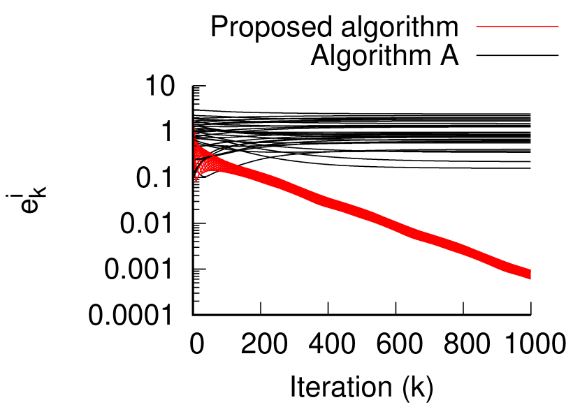
(a)

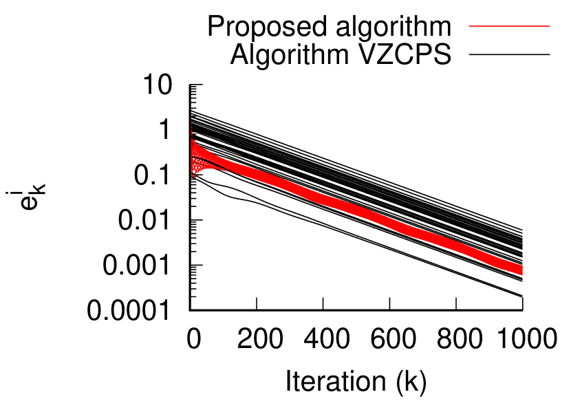
(b)

Figure 1: Effect of modification (12), i.e, removing consensus on variables. (a) Algorithm A does not converge. (b) Algorithm VZCPS, which also introduces modification (15)-(14) converges slower than the proposed one.

In the second experiment we remove modification (12), i.e, add consensus on variables, and study the effect of modification (15)-(14) introduced by Algorithm B. In Figure 2-(a) we see that Algorithm B converges at rate similar to that of the proposed algorithm. However, as explained in Section III, modification (15)-(14) has a negative effect when the minimizing parameters $x_{\star}$ are far from zero. We show this in Figure 2-(b), where we repeat the previous experiment with $x_{\mathrm{true}}=[300,300]^{\top}$. We see how the local estimates of Algorithm B are pulled away from $x_{\star}$ during the initial iterations, until consensus is reached. In Figure 2-(c) we repeat the experiment with $x_{\mathrm{true}}=[1000,1000]^{\top}$. We see that Algorithm B is not able to reach consensus in time, which causes its divergence.

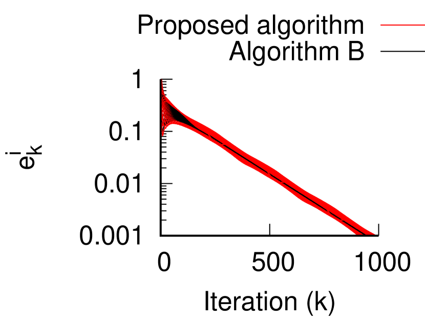
(a)

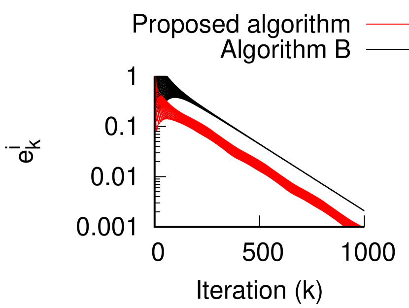
(b)

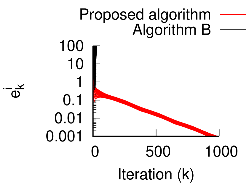
(c)

Figure 2: Effect of modification (15)-(14). (a) With $x_{\mathrm{true}}=[0,0]^{\top}$ Algorithm B performs similar to the proposed one. (b) With $x_{\mathrm{true}}=[300,300]^{\top}$ the parameters are pulled away from $x_{\star}$ until consensus is reached. (c) With $x_{\mathrm{true}}=[1000,1000]^{\top}$ the pulling effect is intensified causing instability.

In the third experiment we evaluate the use of the distributed algorithm for estimating the step size. In Figure 3-(a) we compare the convergence of $\left\|x_{k}^{i}-x_{\star}\right\|$ using both, the optimal step size $\alpha_{\mathrm{opt}}$ and the distributedly estimated one. We see that both methods converge at a very similar rate. We also show in the figure the theoretically optimal rate $\rho^{k}\left(\boldsymbol{\Phi}-\alpha_{\mathrm{opt}}\boldsymbol{\Psi}\right)$. We see that the asymptotic convergence rate of both methods closely resembles the theoretical one. We also show in Figure 3-(b) the evolution of the estimated step size $\alpha_{k}^{i}$ at each node. Finally, Figure 3-(c) shows how the two eigenvalues used to compute $\alpha_{\star}$ depend on $\alpha$, and compares this with the approximated dependence given by Theorem 1. We see how, before the two eigenvalues meet, the true and approximated trajectories closely resemble each other. This results in $\alpha_{\star}=6.117\times 10^{-3}$ being a good approximation of $\alpha_{\mathrm{opt}}=6.197\times 10^{-3}$.

(a)

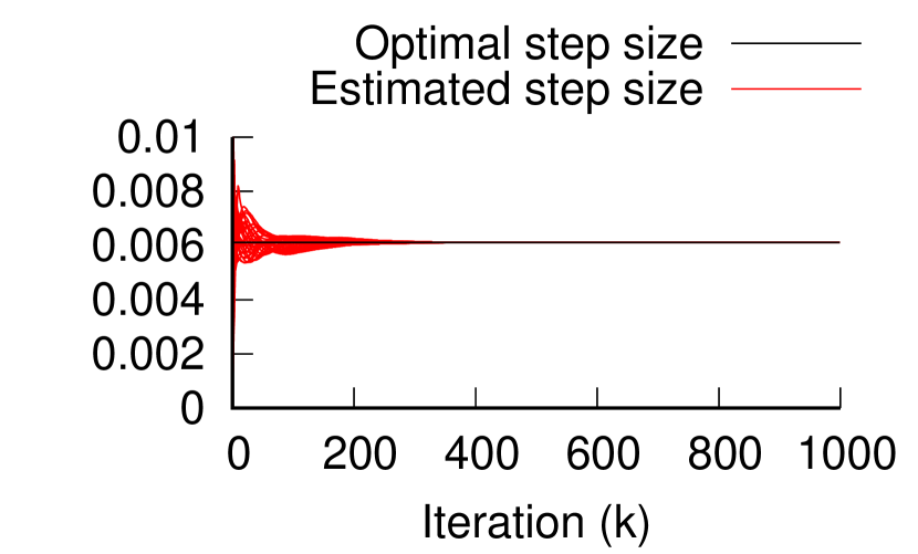
(b)

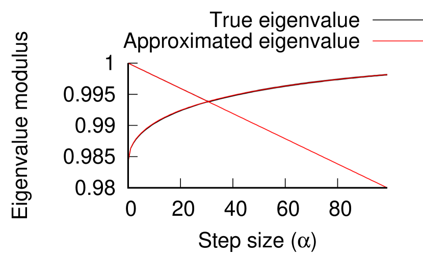
(c)

Figure 3: Distributed estimation of the optimal step size $\alpha_{\star}$. (a) The asymptotic convergence rate matches the theoretically optimal one. (b) Evolution of the distributed step size estimates. (c) Comparison between the actual eigenvalue dependence on the step size and the approximated one.

VII Conclusion

We aimed at achieving the fastest convergence rate for distributed optimization. We did two steps towards this goal. In the first step we proposed a new distributed optimization method which converges faster than other available options. In the second step we proposed a distributed method to estimate the step size that maximizes this rate. We provided sufficient conditions for the convergence of the resulting method in a neighborhood of a local solution. We also provided condition to guarantee global convergence of the method, in the case of an objective function having a single local minimum, together with a different step size selection strategy. We present numerical experiments confirming our claims.

Appendix A Fréchet Derivatives

The Fréchet derivative generalizes the concept of derivative of functions between Euclidean spaces to functions between normed vector spaces [33, 34].

Definition 1.

Let $X$ and $Z$ be normed vector spaces and $U\subseteq X$ be open. A function $f:U\rightarrow Z$ is called Fréchet differentiable at $x\in U$ if there exists a bounded linear map $A:X\rightarrow Z$ such that

$$\lim_{\left\|h\right\|\rightarrow 0}\frac{\left\|f(x+h)-f(x)-A(h)\right\|}{\left\|h\right\|}=0.$$

In this case we say that $A$ is the Fréchet derivative of $f$ at $x$, and denote it by $\mathscr{D}f(x)=A$. We also say that $f$ is Fréchet differentiable if it is so at all $x\in U$. We use $\mathscr{D}f:x\mapsto\mathscr{D}f(x)$ to denote the Fréchet derivative of $f$ and $\mathscr{D}:f\mapsto\mathscr{D}f$ to denote the Fréchet derivation operator.

The $n$-th order Fréchet derivative is the $n$-fold composition of the Fréchet derivation operator, i.e.,

$$\mathscr{D}^{n}f=\underbrace{\mathscr{D}\circ\cdots\circ\mathscr{D}}_{t\text{ times}}f.$$

If $f:X\times Y\rightarrow Z$, we define the partial Fréchet derivative $\mathscr{D}_{x}f(x,y)$ of $f$ with respect to $x$ at $(x,y)$, as the Fréchet derivative of the map $x\mapsto f(x,y)$ at $x$.

As with the derivative of functions between Euclidean spaces, we can approximate a function between normed spaces using a Taylor expansion.

Lemma 5 (Taylor theorem for Fréchet derivatives).

If $f:X\rightarrow Z$ is $n+1$-times continuously differentiable, then

$$f(x+h) =f(x)+\mathscr{D}f(x)(h)+\frac{1}{2!}\mathscr{D}^{2}f(x)(h)(h)+$$

$$\cdots+\frac{1}{n!}\mathscr{D}^{n}f(x)(h)\cdots(h)+O\left(\left\|h\right\|^{n+1}\right).$$

Appendix B Generalized eigenvalue problem

Given a matrix pair $A,B\in\mathbb{R}^{N\times N}$, the generalized eigenvalue problem consists in finding the values of $\lambda\in\mathbb{C}$, satisfying

$$\det\left(A-\lambda B\right)=0.$$

We say that $x,y\in\mathbb{R}^{N}$ are, respectively, right and left generalized eigenvectors associated with $\lambda$ if

$$Ax =\lambda Bx,$$

$$y^{\top}A =\lambda y^{\top}B.$$

The following result gives an approximation of the perturbation $\tilde{\lambda}$ of a generalized eigenvalue $\lambda$, when matrix $A$ is modified by adding to it a perturbation matrix $\tilde{A}$.

Lemma 6.

Let $x$ and $y$ be right and left generalized eigenvectors of $A,B\in\mathbb{R}^{N\times N}$ associated with $\lambda$ and

$$\left(A+\tilde{A}\right)\left(x+\tilde{x}\right)=\left(\lambda+\tilde{\lambda}\right)B\left(x+\tilde{x}\right).$$

Then

$$\tilde{\lambda}=\frac{y^{\top}\tilde{A}\left(x+\tilde{x}\right)}{y^{\top}B\left(x+\tilde{x}\right)}.$$

Proof:

We have

$$\left(A+\tilde{A}\right)\left(x+\tilde{x}\right) =\left(\lambda+\tilde{\lambda}\right)B\left(x+\tilde{x}\right) \Rightarrow$$

$$Ax+\tilde{A}x+A\tilde{x}+\tilde{A}\tilde{x} =\lambda Bx+\tilde{\lambda}Bx+\lambda B\tilde{x}+\tilde{\lambda}B\tilde{x} \Rightarrow$$

$$\tilde{A}x+A\tilde{x}+\tilde{A}\tilde{x} =\tilde{\lambda}Bx+\lambda B\tilde{x}+\tilde{\lambda}B\tilde{x} \Rightarrow$$

$$\tilde{A}\left(x+\tilde{x}\right)+A\tilde{x} =\tilde{\lambda}B\left(x+\tilde{x}\right)+\lambda B\tilde{x}$$

Then

$$0 =y^{\top}\tilde{A}\left(x+\tilde{x}\right)+y^{\top}A\tilde{x}-\tilde{\lambda}y^{\top}B\left(x+\tilde{x}\right)-\lambda y^{\top}B\tilde{x}$$

$$=y^{\top}\tilde{A}\left(x+\tilde{x}\right)+y^{\top}\left(A-\lambda B\right)\tilde{x}-\tilde{\lambda}y^{\top}B\left(x+\tilde{x}\right)$$

$$=y^{\top}\tilde{A}\left(x+\tilde{x}\right)-\tilde{\lambda}y^{\top}B\left(x+\tilde{x}\right),$$

and the result follows. ∎

Appendix C Distributed estimation $\lambda_{2}$ and $u$ in the case of undirected communication graphs

In this section we describe a distributed method for estimating $\lambda_{2}$ and $u$ in the case where the graph induced by the communication network is undirected.

We know that $1$ is the largest eigenvalue of $W$ with (left and right) eigenvector $\mathbf{1}_{I}$. Hence,

$$V=W-\frac{1}{I}\mathbf{1}_{I}\mathbf{1}_{I}^{\top},$$

has $\lambda_{2}$ as its largest eigenvalue with eigenvector $v$. We can then obtain recursive estimates $\hat{\lambda}_{2,k}$ and $\hat{u}_{k}$ , of $\lambda_{2}$ and $u$, using the power method. To this end, an initialization random vector $\hat{u}_{1}$ is produced by locally drawing each random entry at each node, and the following iterations are run

$$\hat{u}_{k+1} =V\hat{u}_{k}$$

$$=W\hat{u}_{k}-\mathbf{1}_{I}\bar{u}.$$

In order to run the above, we need a recursive estimate $\hat{\bar{u}}_{k}$ of $\bar{u}$ at each node. We also obtain so using the power method, i.e., we put $\hat{\bar{u}}_{1}=\hat{u}_{1}$ and run

$$\hat{\bar{u}}_{k+1}=W\hat{\bar{u}}_{k}.$$

The estimation of $\lambda_{2}$ is then obtained as follows

$$\hat{\lambda}_{2,k}=\frac{\left\|\hat{u}_{k}\right\|}{\left\|\hat{u}_{k-1}\right\|}.$$

References

- [1] Jin-Jun Xiao, Alejandro Ribeiro, Zhi-Quan Luo, and Georgios B Giannakis. Distributed compression-estimation using wireless sensor networks. IEEE Signal Proces Magazine, 23(4):27–41, 2006.
- [2] D Marelli and M Fu. Distributed weighted least-squares estimation with fast convergence for large-scale systems. Automatica, 51:27–39, 2015.
- [3] Alejandro Ribeiro, Ioannis D Schizas, Stergios I Roumeliotis, and Georgios Giannakis. Kalman filtering in wireless sensor networks. IEEE Control Systems Magazine, 30(2):66–86, 2010.
- [4] Paolo Massioni and Michel Verhaegen. Distributed control for identical dynamically coupled systems: A decomposition approach. IEEE Transactions on Automatic Control, 54(1):124–135, 2009.
- [5] Raffaello D’Andrea and Geir E Dullerud. Distributed control design for spatially interconnected systems. IEEE Transactions on Automatic Control, 48(9):1478–1495, 2003.
- [6] Tao Yang, Xinlei Yi, Junfeng Wu, Ye Yuan, Di Wu, Ziyang Meng, Yiguang Hong, Hong Wang, Zongli Lin, and Karl H Johansson. A survey of distributed optimization. Annual Reviews in Control, 2019.
- [7] Ali H Sayed. Adaptation, learning, and optimization over networks. Foundations and Trends in Machine Learning, 7:311–801, 2014.
- [8] Angelia Nedić and Ji Liu. Distributed optimization for control. Annual Review of Control, Robotics, and Autonomous Systems, 1:77–103, 2018.
- [9] Angelia Nedich. Convergence rate of distributed averaging dynamics and optimization in networks. Foundations and Trends in Systems and Control, 2(1):1–100, 2015.
- [10] Bo Yang and Mikael Johansson. Distributed optimization and games: A tutorial overview. In Networked Control Systems, pages 109–148. Springer, 2010.
- [11] M. Gürbüzbalaban, A. Ozdaglar, and P. Parrilo. A globally convergent incremental newton method. Math Program, 151(1):283–313, 2015.
- [12] S Boyd, N Parikh, E Chu, B Peleato, and J Eckstein. Distributed optimization and statistical learning via the alternating direction method of multipliers. Found Trends Machine learning, 3(1):1–122, 2011.
- [13] Ermin Wei and Asuman Ozdaglar. Distributed alternating direction method of multipliers. In 2012 IEEE 51st IEEE Conference on Decision and Control (CDC), pages 5445–5450. IEEE, 2012.
- [14] A. Nedic and A. Ozdaglar. Distributed subgradient methods for multi-agent optimization. IEEE Trans. Autom. Control, 54(1):48–61, 2009.
- [15] Dušan Jakovetić, Joao Xavier, and José MF Moura. Fast distributed gradient methods. IEEE Trans. Autom. Control, 59(5):1131–1146, 2014.
- [16] Kun Yuan, Qing Ling, and Wotao Yin. On the convergence of decentralized gradient descent. SIAM J. Optim., 26(3):1835–1854, 2016.
- [17] Wei Shi, Qing Ling, Gang Wu, and Wotao Yin. Extra: An exact first-order algorithm for decentralized consensus optimization. SIAM Journal on Optimization, 25(2):944–966, 2015.
- [18] Tao Yang, Yan Wan, Hong Wang, and Zongli Lin. Global optimal consensus for discrete-time multi-agent systems with bounded controls. Automatica, 97:182–185, 2018.
- [19] S. Pu, W. Shi, J. Xu, and A. Nedic. Push-pull gradient methods for distributed optimization in networks. IEEE Trans. Autom. Control, 2020.
- [20] A Mokhtari, Q Ling, and A Ribeiro. Network newton distributed optimization methods. IEEE T Signal Proc, 65(1):146–161, 2016.
- [21] F Mansoori and E Wei. A fast distributed asynchronous newton-based optimization algorithm. IEEE T Autom Control, 2019.
- [22] Rasul Tutunov, Haitham Bou-Ammar, and Ali Jadbabaie. Distributed newton method for large-scale consensus optimization. IEEE Transactions on Automatic Control, 64(10):3983–3994, 2019.
- [23] A Jadbabaie, A Ozdaglar, and M Zargham. A distributed newton method for network optimization. In IEEE CDC, pages 2736–2741. IEEE, 2009.
- [24] D. Varagnolo, F. Zanella, A. Cenedese, G. Pillonetto, and L. Schenato. Newton-raphson consensus for distributed convex optimization. IEEE Transactions on Automatic Control, 61(4):994–1009, 2016.
- [25] Filippo Zanella, Damiano Varagnolo, Angelo Cenedese, Gianluigi Pillonetto, and Luca Schenato. Newton-raphson consensus for distributed convex optimization. In IEEE CDC, pages 5917–5922. IEEE, 2011.
- [26] F. Zanella, D. Varagnolo, A. Cenedese, G. Pillonetto, and L. Schenato. Asynchronous newton-raphson consensus for distributed convex optimization. IFAC Proceedings Volumes, 45(26):133–138, 2012.
- [27] Nicoletta Bof, Ruggero Carli, Giuseppe Notarstefano, Luca Schenato, and Damiano Varagnolo. Multiagent newton–raphson optimization over lossy networks. IEEE Trans. Autom. Control, 64(7):2983–2990, 2018.
- [28] Y. Li, H. Zhang, B. Huang, and J. Han. A distributed newton–raphson-based coordination algorithm for multi-agent optimization with discrete-time communication. Neural Comput Appl, pages 1–15, 2018.
- [29] Jiaqi Zhang, Keyou You, and Tamer Başar. Distributed adaptive newton methods with globally superlinear convergence. arXiv preprint arXiv:2002.07378, 2020.
- [30] R. Olfati-Saber, J Fax, and R. Murray. Consensus and cooperation in networked multi-agent systems. Proc. IEEE, 95(1):215–233, 2007.
- [31] Minghui Zhu and Sonia Martínez. Discrete-time dynamic average consensus. Automatica, 46(2):322–329, 2010.
- [32] Thomas P Wihler. On the hölder continuity of matrix functions for normal matrices. Journal of inequalities in pure and applied mathematics, 10:1–5, 2009.
- [33] Richard S Hamilton et al. The inverse function theorem of nash and moser. B Am Math Soc, 7(1):65–222, 1982.
- [34] Rodney Coleman. Calculus on normed vector spaces. Springer Science & Business Media, 2012.